Validation of RANS-calibrated engineering models and ANN-based surrogate for wind farm flow simulation and layout optimization

Accurate yet efficient wake modeling is essential for wind farm layout optimization (WFLO). Wind turbine wakes are disturbed regions of flow behind a wind turbine, characterized by lower mean wind speeds and higher turbulence, which reduce downstream power production and increase structural loading. This study compares an artificial neural network (ANN)-based surrogate trained on Reynolds-averaged Navier–Stokes (RANS) data with two representative engineering wake models based on the TurbOPark and super-Gaussian formulations. The work includes recalibration of the engineering models, a systematic flow simulation study across varying turbine counts and spacings, and WFLO benchmarks validated against RANS-based annual energy production (AEP). Results show that the ANN surrogate achieves the lowest RMSE and MAPE across all scenarios in flow estimation, albeit at a higher computational cost. In WFLO, the TurbOPark-based model produced the highest RANS-validated AEP layouts, despite having lower predictive accuracy, suggesting that optimization complexity influences outcomes. Blockage modeling increased computational cost without improving accuracy.

1 Introduction

A key challenge when designing a wind farm is determining the optimal placement of wind turbines. This decision must consider various factors, including nearby communities, local wind conditions, electrical infrastructure, seabed conditions, and other relevant considerations. The interaction between turbines through wake effects is particularly important, as it can significantly reduce energy output and, in turn, impact project economic viability. While wake effects are the dominant turbine-to-turbine interaction, the induction of the turbines also produces a wind-farm-scale blockage effect that slows the inflow upstream and can result in power losses at the leading turbines (Bleeg et al., 2018). This upstream slowdown has been observed in offshore lidar measurements (Schneemann et al., 2021) and grows in relevance for the large turbine counts of modern offshore wind farms, where the induction of the individual turbines aggregates into a combined wind-farm-scale blockage effect (Nygaard et al., 2020).

To obtain the best achievable placement of the turbines, wind farm layout optimization (WFLO) can be applied. WFLO utilizes numerical optimization to minimize or maximize a given cost function, typically a variation of energy production or energy cost, while adhering to predefined constraints (see, e.g., Herbert-Acero et al., 2014; Baker et al., 2019; Bortolotti et al., 2022). WFLO algorithms can be broadly grouped into gradient-based and gradient-free methods. The present work focuses on gradient-based optimization. Gradient-free approaches nonetheless remain an area of interest and continue to advance, ranging from classical evolutionary genetic algorithms (Mosetti et al., 1994) and particle swarm optimization (Pookpunt and Ongsakul, 2013) to recent hybrids such as the reinforcement learning-enhanced genetic algorithm of Dong et al. (2026). Regardless of the optimization algorithm applied in WFLO, it is essential for flow models to account for wake effects. Existing approaches can be broadly classified into two categories: engineering wake models, which construct the wind farm flow field by superposing individual wakes, and computational fluid dynamics (CFD) models, which resolve the underlying physics through numerical simulation.

The first engineering model, proposed by Jensen (1983) and often referred to as the Park model, was primarily concerned with representing the wake-center velocity and employed a top-hat shape to do so. This approximation initially worked well but became increasingly problematic as the turbine and wind farm sizes increased. The breakdown of turbulent structures leads to the wake becoming self-similar and converging toward a Gaussian-like shape. For this reason, later variations typically rely on a Gaussian profile to model the wake deficits. The area where the wake is self-similar is referred to as the far wake. The location downstream of the turbine where this occurs depends on both atmospheric and terrain conditions. Dar et al. (2019) investigated this with LESs and showed that self-similarity occurs between 1–3 rotor diameters (D) in complex terrain and between 3–10 rotor diameters for flat terrain. The different areas of the flow around a wind turbine are labeled and illustrated in Fig. 1.

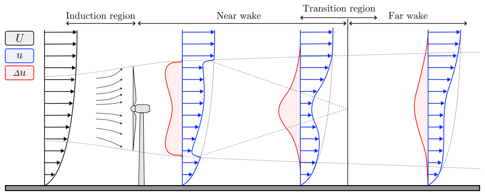
Figure 1 Simplified illustration of the flow around a wind turbine, depicting the upstream induction zone and the downstream wake, which is separated into the near wake, transition region, and far wake. The illustration includes the effective wind speed and the velocity deficit, illustrating the influence of the turbine on the background flow.

In the literature, engineering models and CFD methods are often referred to as low- and high-fidelity models, respectively. Engineering models are much faster: $\sim {\mathrm{10}}^{\mathrm{4}}\times$ faster than Reynolds-averaged Navier–Stokes (RANS) (van der Laan et al., 2015a) and $\sim {\mathrm{10}}^{\mathrm{7}}\times$ faster than large-eddy simulation (LES) (Porté-Agel et al., 2020), making CFD too slow for WFLO, where the flow must be evaluated many times during the optimization process. In general, high-fidelity models are considered more accurate. However, under certain circumstances, engineering models can outperform high-fidelity models, e.g., within limited domains, such as the far wake, when operating near a calibration point, or when considering integrated quantities, such as power. However, design decisions and the calibration domain constrain their upper limits of accuracy.

Wake models can be split into two categories. The first comprises analytically solved models, which typically assume a self-similar far-wake profile. Alternatively, there is a group of low-fidelity models that require solving but do not rely on self-similarity profiles (e.g., Ainslie, 1988; Ott et al., 2011; Klemmer and Howland, 2025). The class of self-similar, analytically solved wake models dominates WFLO practice and is the focus of the present study. In WFLO, a minimum inter-turbine separation is typically imposed to limit fatigue loads; because this constraint keeps downstream turbines out of the near wake, engineering wake models applied in WFLO have typically been developed and calibrated with the far wake as the design target.

Several analytically solved engineering models exist and can loosely be categorized into families: Gaussian formulations (Bastankhah and Porté-Agel, 2014; Niayifar and Porté-Agel, 2016), a super-Gaussian variation that bridges top-hat near-wake and Gaussian far-wake behavior (Blondel and Cathelain, 2020), and the turbulence-optimized park (TurbOPark) models (Nygaard et al., 2020, 2022). Special formulations have also been developed to account for the wake of turbines operating with a yaw offset, which is particularly useful for wake-steering scenarios (Bastankhah and Porté-Agel, 2016; Martínez-Tossas et al., 2019). The breadth of existing models is wide, and the models mentioned here are an important subset, but many more exist for different applications. At the farm scale, overlapping wakes have further motivated momentum-conserving superposition schemes (Zong and Porté-Agel, 2020; Lanzilao and Meyers, 2022) beyond the classical linear and quadratic sums (Porté-Agel et al., 2020). In the present study, recalibration has been performed on two engineering model configurations using the PyWake (Pedersen et al., 2023) framework.

An alternative to classical models is the use of data-driven surrogate models. Surrogates are models that seek to approximate a higher-fidelity model at a fraction of the cost. In wake modeling, surrogates are typically trained with RANS or LES data. Zehtabiyan-Rezaie et al. (2022) have conducted a review of the field, encompassing various types of artificial neural network (ANN)-based wake surrogates, as well as classic machine learning (ML) techniques such as proper orthogonal decomposition (POD) and dynamic mode decomposition (DMD). Some notable works include Ti et al. (2021) and Yang and Deng (2023), who trained an ANN-based RANS surrogate using multiple parallel neural networks, each corresponding to a specific grid location in the turbine flow. A limitation of this approach is that the surrogate cannot be used with automatic differentiation in gradient-based WFLO or any optimization with continuous turbine coordinates, as these models are undefined outside the considered grid points. To address this, we have previously developed ANN-based RANS surrogates with continuous definitions that support automatic differentiation (Schøler et al., 2023; Pish et al., 2024). One limitation of training ANN-based surrogates is the need for extensive data to cover cases across various inflow types and operating conditions. Schøler et al. (2024) investigated physics-informed neural networks (PINNs) as a means to reduce data requirements, ultimately finding that a hybrid data-and-physics loss was too costly given the gains. Gafoor et al. (2025) demonstrated the possibility of an RANS PINN surrogate trained solely with physics information. Together, current literature indicates a significant potential in ANN-based RANS surrogates. From the related field of dynamic surrogate wake models, a couple of interesting works are listed to situate the current work better in a wider context. Dynamic models are typically motivated by a desire to improve wind farm control and mitigate loads. The work of Zhang and Zhao (2021) used a physics-informed reconstruction of unsteady wake fields from lidar measurements, the predictive and stochastic reduced-order model (PS-ROM) of wake dynamics by Andersen and Leon (2022), the PS-ROM derivative work on global POD modes by Moreno et al. (2025), and real-time physics-guided frameworks (Li et al., 2024a). Most recently, Liu et al. (2026) proposed PhyWakeNet, a hybrid physics and data-driven model that captures the time-averaged deficit, wake meandering, and small-scale turbulence of an unsteady wake using separate but integrated model components.

While numerous studies on ANN wake surrogates hypothesize that these models can outperform traditional engineering approaches in flow simulation and WFLO accuracy, numeric validation studies remain limited. Anagnostopoulos and Piggott (2022) trained an ANN surrogate using data from an engineering model and applied it to both yaw optimization for a 15-turbine array and layout optimization for a 6-turbine configuration. Similarly, Sun and Yang (2023) developed an ANN surrogate trained on data from an engineering model and conducted a WFLO study incorporating hub-height optimization for a 30-turbine wind farm. Yang et al. (2022) and Yang and Deng (2023) demonstrated the ANN-RANS surrogates developed by Ti et al. (2021) in yaw optimization of a five-turbine row and in a WFLO re-powering study of the Horns Rev 1 offshore wind farm, respectively. However, neither study validated their results against CFD simulations or against supervisory control and data acquisition (SCADA) data. In contrast, Li et al. (2024b) introduced a novel RANS-based ANN surrogate trained using a generative adversarial network (GAN). Their study included flow simulation via the superposition of single-wake models applied to the Horns Rev 1 wind farm, with power production results compared against RANS, time-averaged LES, and SCADA data, though only for a limited range of inflow cases. Likewise, Liu et al. (2025) trained a convolutional neural network (CNN) surrogate using time-averaged LES data and validated it using time-averaged LES simulations from a row of five turbines with varying inter-turbine spacings.

In summary, the existing validation studies in the literature have been limited by surrogate training and validation using low-fidelity engineering model data, WFLO without validation, flow studies with few turbines or limited variation in the studied farm layouts, and restricted inflow conditions. In this work, systematic experiments are conducted to validate a pre-developed RANS-ANN for flow simulation and WFLO. The contributions of this work include the following two main items, a flow study and a WFLO study:

• 1a.

  recalibration of engineering models to a RANS-based single-wake dataset;

• 1b.

  comparative study investigating the accuracy of an ANN wake model and two popular engineering model setups for wind farm flow simulation with a varying number of wind turbines, including a cost–benefit analysis of accuracy, memory consumption, and computational cost;

• 2.

  WFLO validation study of the ANN wake model against two engineering model setups and three different optimization algorithms, as well as validation of the optimized layouts with RANS-based annual energy production (AEP) estimates.

The paper consists of Sect. 2, which outlines the studies conducted and the methods used. In Sect. 3, the results of the studies are presented and discussed. In Sect. 4, the conclusions of the study are summarized, and suggestions for future work are presented.

2 Methodology

In this section, the methods used in the paper are presented, and the experiments conducted are described.

2.1 Reynolds-averaged Navier–Stokes (RANS)

RANS is a steady-state CFD model that solves the mean flow by modeling all turbulence scales. As RANS represents the time-averaged wake, it does not resolve unsteady features such as wake meandering, whose net effect on the mean velocity deficit and wake recovery is instead represented implicitly through a calibrated closure model, here the k–ε–f_P (van der Laan et al., 2015a, b).

The inflow represents a logarithmic profile, where the ambient turbulence intensity (TI) based on the turbulent kinetic energy at hub height is set by the roughness length. For the WFLO AEP study, the TI is set to 6 %, yielding an offshore roughness length of $\mathrm{2.5}\times {\mathrm{10}}^{-\mathrm{4}}$ m. The turbines are modeled by actuator disks (ADs) (Troldborg et al., 2015). The AD thrust and tangential force distributions utilize an analytical Joukowsky rotor model, as proposed by Sørensen et al. (2020) but recalibrated by van der Laan et al. (2020) for improved performance under veer and shear. The RANS simulations are performed with the PyWakeEllipsys code (DTU Wind and Energy Systems, 2023), which wraps the EllipSys3D finite-volume flow solver (Michelsen, 1992; Sørensen, 1994).

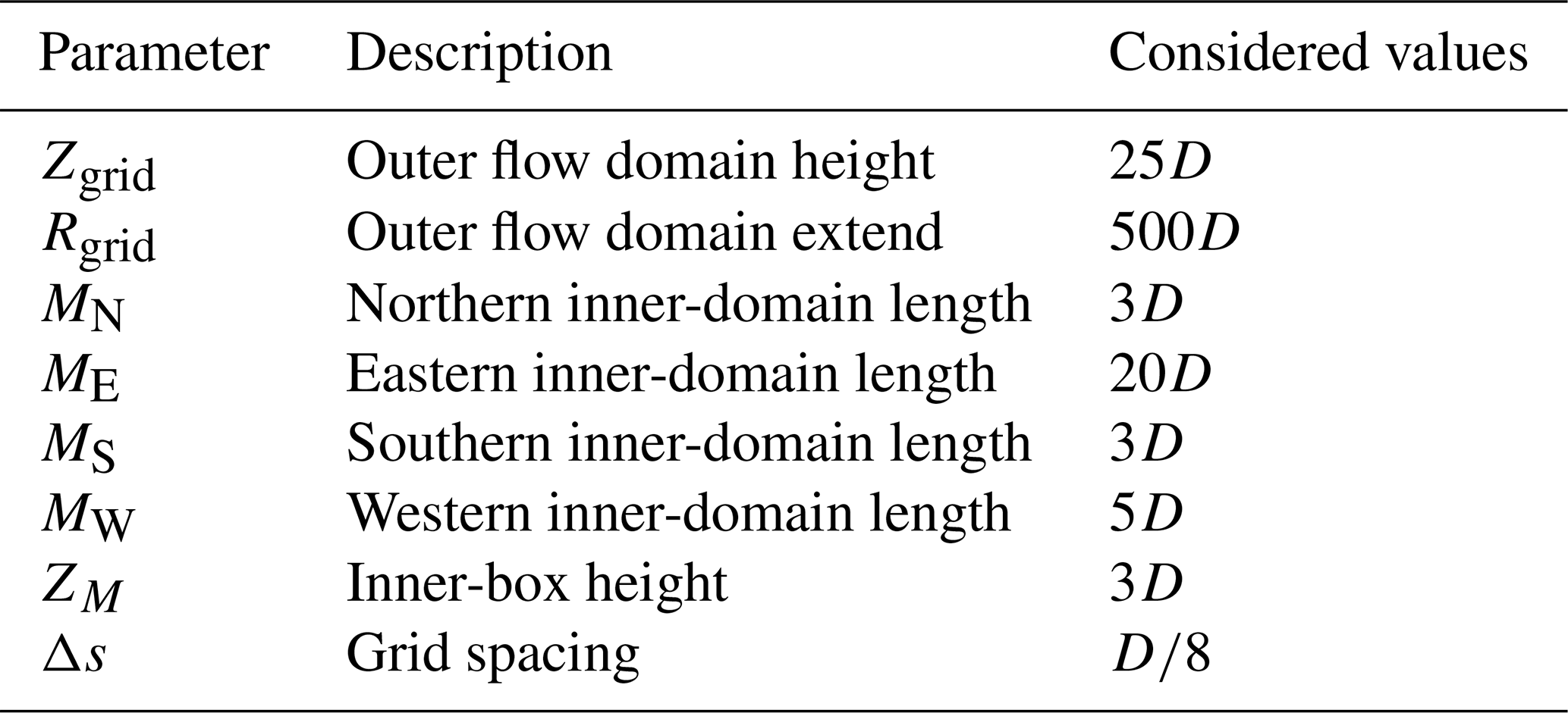
A Cartesian mesh with inner and outer grids was used, as illustrated in Fig. 2. The mesh is fixed with the inflow always directed from west to east, and different wind directions are realized by rotating the wind farm layout rather than the grid. Generic mesh parameters are introduced in Fig. 2, and their specific values are listed in Table 1. The asymmetric extents, M_E=20D downstream, $M_{\mathrm{N}}=M_{\mathrm{S}}=\mathrm{3}D$ lateral, and M_W=5D upstream, follow from this orientation: only the downstream direction requires a large buffer to capture the far wake.

Figure 2 Illustration of utilized PyWakeEllipsys-flatbox mesh.

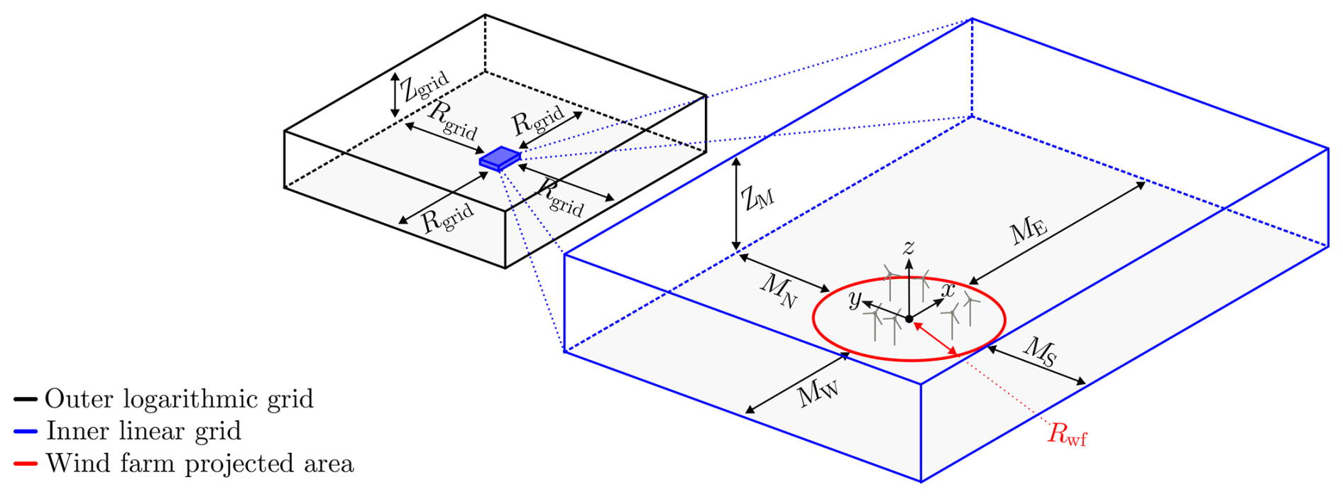
Table 1 Parameters for PyWakeEllipSys-flatbox mesh considered during simulations.

The WFLO RANS AEP simulations are performed for all wind directions and wind speeds with intervals of 5° and 1 m s⁻¹, respectively, yielding 1584 inflow cases. The simulations are run consecutively, where each new wind speed is obtained by scaling the turbine controllers according to Reynolds number similarity (van der Laan et al., 2019), while the inflow is kept constant. This reduces the total number of required iterations because only local changes need to be recalculated, as discussed by van der Laan et al. (2022). Furthermore, the wind speed cases are simulated from low to high, and the wind speed cases above the wind farm rated wind speed are skipped, which reduce the total number of flow cases by about 40 %. Finally, a relatively low convergence level of 10⁻⁴ is applied, which reduces the computational effort by an order of magnitude, while the convergence error in terms of AEP is 0.02 %, as shown in van der Laan et al. (2022). A single AEP simulation with this RANS setup takes between 28–33 h employing 1000 cores using the Sophia high-performance computer (HPC) (Technical University of Denmark, 2019), which is equipped with first-generation AMD EPYC 7351 cores (released in 2017). Tests of PyWakeEllipSys RANS simulations on a different HPC with more modern fourth-generation AMD Genoa-X cores (released in 2023) shows a speed-up of a factor of 2.

2.2 Engineering models

In this work, the PyWake engineering model framework (Pedersen et al., 2023) was used as the engine to run wind farm simulations. PyWake is a highly efficient framework that provides a high degree of abstraction for the components commonly found in low-fidelity wind farm models. The vast number of module combinations means only a subset can be considered at a time. We have chosen to consider a configuration based on the Turbulence Optimized Park model (TurbOPark) (Nygaard et al., 2020, 2022). The configuration is altered slightly and is therefore generally referred to as the TP model to avoid confusion with the original TurbOPark (Nygaard et al., 2022). The second alternative considered is based on a configuration submitted to the American WAKE Experiment (AWAKEN) (Bodini et al., 2026), which utilizes the super-Gaussian model proposed by Blondel and Cathelain (2020) and is therefore referred to as the SG model.

Regardless of the wake model used to represent the wind farm flow field, wake superposition is required. This is typically performed using either linear or quadratic methods. In the present work, linear superposition is applied for velocity deficits (Δu) in both configurations, while a quadratic max sum is used for added turbulence intensity (I_a) in the SG configuration. An overview of superposition methods is provided by Porté-Agel et al. (2020).

For readers already familiar with engineering wind farm models, a summary of the two configurations is shown in Table 2, while the models are presented in greater detail in the remainder of the subsection for readers who are unfamiliar with them. Where possible, the PyWake default superposition model has been used. In the TP configuration, however, the wake and blockage models require different superposition methods: the original TurbOPark model superimposes the wake deficits quadratically (Nygaard et al., 2022), but a quadratic (squared) sum would not preserve the sign of the blockage-induced speed-ups (Forsting et al., 2023). Linear superposition is therefore applied to the velocity deficits so that the wake and blockage contributions can be combined under a single operator.

Blondel and Cathelain (2020)Nygaard et al. (2022)Forsting et al. (2023)Forsting et al. (2023)Crespo and Hernández (1996)Crespo and Hernández (1996)

Table 2 Comparison of PyWake configurations (with/without blockage). Values flanked by dashes indicate shared settings across both blockage configurations. A single dash (–) indicates that the component is not used.

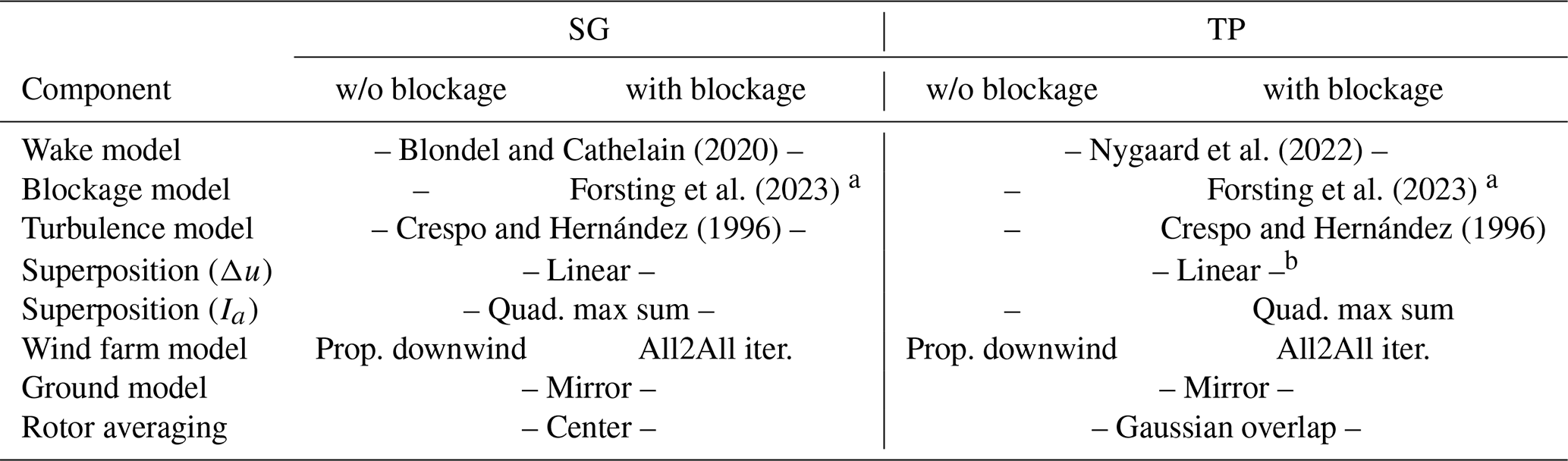
^a Updated version of Troldborg and Meyer Forsting (2017).
^b In the original TurbOPark paper, quadratic superposition was employed; however, this approach is incompatible with the blockage model (Forsting et al., 2023).

Turbo Park (TP) model

The TP model uses the updated Turbulence Optimized Park (TurbOPark) model (Nygaard et al., 2022), a Gaussian wake model derived from the classic Gaussian wake model by (Bastankhah and Porté-Agel, 2014). The wake model is shown in Eq. (1):

$$\begin{array}{}\text{(1a)}& {\displaystyle }& {\displaystyle \frac{\mathrm{\Delta }u\left(x\right)}{U}}=C\left(x\right)\exp \left(-{\displaystyle \frac{r^{\mathrm{2}}}{\mathrm{2}{\mathit{\sigma }}_w^{\mathrm{2}}\left(x\right)}}\right),\text{(1b)}& {\displaystyle }& {\displaystyle }C\left(x\right)=\mathrm{1}-\sqrt{\mathrm{1}-{\displaystyle \frac{C_{\mathrm{T}}}{\mathrm{8}\left({\mathit{\sigma }}_w\right(x)/D{)}^{\mathrm{2}}}}},\end{array}$$

where Δu(x) is the wake deficit at the downstream position x, U is the free-stream velocity, C(x) is the peak velocity deficit at the wake centerline, r is the radial distance from the wake center, C_T is the coefficient of thrust, and σ_w(x) is the variable wake expansion factor, which is the major difference between the TurbOPark implementation and the default Gaussian deficit model which uses a constant wake expansion factor. The expression for the wake expansion factor σ_w(x) is implemented using the Frandsen (2005) turbulence model, which is why the TurbOPark model does not require a standalone added-turbulence model. σ_w(x) is shown in Eq. (2) parameterized with α and β from Frandsen (2005):

$$\begin{array}{ll}{\displaystyle }& {\displaystyle \frac{{\mathit{\sigma }}_w\left(x\right)}{D}}=\mathit{\epsilon }+{\displaystyle \frac{A{I}_{\mathrm{0}}}{\mathit{\beta }}}\cdot \left(\sqrt{{\left(\mathit{\alpha }+\mathit{\beta }x/D\right)}^{\mathrm{2}}+\mathrm{1}}-\sqrt{\mathrm{1}+{\mathit{\alpha }}^{\mathrm{2}}}\right.\\ \text{(2a)}& {\displaystyle }& {\displaystyle }\left.-\ln \left[{\displaystyle \frac{\left(\sqrt{{\left(\mathit{\alpha }+\mathit{\beta }x/D\right)}^{\mathrm{2}}+\mathrm{1}}+\mathrm{1}\right)\mathit{\alpha }}{\left(\sqrt{\mathrm{1}+{\mathit{\alpha }}^{\mathrm{2}}}+\mathrm{1}\right)\left(\mathit{\alpha }+\mathit{\beta }x/D\right)}}\right]\right),\text{(2b)}& {\displaystyle }& {\displaystyle }\mathit{\alpha }:=c_{I,\mathrm{1}}{I}_{\mathrm{0}},\mathit{\beta }:={\displaystyle \frac{c_{I,\mathrm{2}}{I}_{\mathrm{0}}}{\sqrt{C_{\mathrm{T}}}}}{\displaystyle }& {\displaystyle }\mathit{\epsilon }:=c_{\mathit{\epsilon }}\sqrt{{\displaystyle \frac{\mathrm{1}}{\mathrm{2}}}{\displaystyle \frac{\mathrm{1}+\sqrt{\mathrm{1}-{\widehat{C}}_{\mathrm{T}}}}{\sqrt{\mathrm{1}-{\widehat{C}}_{\mathrm{T}}}}}},\\ \text{(2c)}& {\displaystyle }& {\displaystyle }\text{where }{\widehat{C}}_{\mathrm{T}}:=min(C_{\mathrm{T}},C_{\text{T,\hspace{0.17em}lim}}),\end{array}$$

where I₀ is the ambient TI, A is a wake expansion calibration parameter, c_I,1 and c_I,2 are calibration parameters from the Frandsen (2005) model, and ε is an initial characteristic wake width; i.e., ${\mathit{\sigma }}_w\left(\mathrm{0}\right)/D=\mathit{\epsilon }$. Here, it is important to note that the engineering wake models operate under an assumption that I_k=I_u, where $I_k=\sqrt{\mathrm{2}/\mathrm{3}\cdot k}/U$ is the TI derived from turbulent kinetic energy, and $I_u={\mathit{\sigma }}_u/U$ is the streamwise TI based on the standard deviation (SD) of the flow in the streamwise direction σ_u. This differs from the more physically accurate relationship $I_k\approx \mathrm{0.8}\cdot I_u$, derived from standard atmospheric turbulence ratios (Panofsky and Dutton, 1984). However, this simplification is not expected to alter the main conclusions, as the recalibrated models exhibit similar overall trends.

Super-Gaussian (SG) model

The SG model, as previously mentioned, uses the super-Gaussian model proposed by Blondel and Cathelain (2020); here, we present the simplified analytical version. The model unifies the observation that the far wake can be accurately modeled as a Gaussian shape, whereas the near wake more closely resembles a top-hat shape. By augmenting the super-Gaussian shape parameter n, the velocity deficit takes on different forms; i.e., when n=2, it becomes a regular Gaussian shape, while for n>2 the shape gradually becomes more top-hat-like.

$$\begin{array}{}\text{(3a)}& {\displaystyle }& {\displaystyle \frac{\mathrm{\Delta }u\left(x\right)}{U}}=C\left(x\right)\exp \left(-{\displaystyle \frac{(r/D{)}^n}{\mathrm{2}\left(\mathit{\sigma }\right(x)/D{)}^{\mathrm{2}}}}\right)\text{(3b)}& {\displaystyle }& {\displaystyle }C\left(x\right)={\mathrm{2}}^{\mathrm{2}/n-\mathrm{1}}-\sqrt{{\mathrm{2}}^{\mathrm{4}/n-\mathrm{2}}-{\displaystyle \frac{n{C}_{\mathrm{T}}}{\mathrm{16}\mathrm{\Gamma }(\mathrm{2}/n)\left(\mathit{\sigma }\right(x)/D{)}^{\mathrm{4}/n}}}}\text{(3c)}& {\displaystyle }& {\displaystyle \frac{\mathit{\sigma }\left(x\right)}{D}}=(a_{s}I+b_s)x/D+c_s\sqrt{{\displaystyle \frac{\mathrm{1}}{\mathrm{2}}}{\displaystyle \frac{\mathrm{1}+\sqrt{\mathrm{1}-C_{\mathrm{T}}}}{\sqrt{\mathrm{1}-C_{\mathrm{T}}}}}}\text{(3d)}& {\displaystyle }& {\displaystyle }n\approx a_f\exp \left(b_f\cdot x/D\right)+c_f,a_f:=\mathrm{3.11}\end{array}$$

Here Γ is the gamma function, and I is the effective TI. Equation (3d) shows the exponential function that Blondel and Cathelain (2020) created to avoid having to solve for n and is the key change to enable fast evaluations of the flow. The effective TI is evaluated using the added-TI (I_a) model proposed by Crespo and Hernández (1996) and the quadratic sum. The Crespo and Hernández (1996) model is shown in Eq. (4). To evaluate the axial induction (a_m), the method by Madsen et al. (2020), as implemented in PyWake, is utilized, and a quadratic max summation is used for superposition:

$$\begin{array}{}\text{(4a)}& {\displaystyle }& {\displaystyle }{I}_{\mathrm{a}}=\mathrm{0.73}{a}_{\mathrm{m}}^{\mathrm{0.8325}}{I}_{\mathrm{0}}^{-\mathrm{0.0325}}{\left(x/D\right)}^{-\mathrm{0.32}},\text{(4b)}& {\displaystyle }& {\displaystyle }{a}_{\mathrm{m}}=\mathrm{0.083}{C}_{\mathrm{T}}^{\mathrm{3}}+\mathrm{0.0586}{C}_{\mathrm{T}}^{\mathrm{2}}+\mathrm{0.2460}{C}_{\mathrm{T}},\text{(4c)}& {\displaystyle }& {\displaystyle }I=\sqrt{I_{\mathrm{0}}^{\mathrm{2}}+\underset{j}{max}(I_{\mathrm{a},j}{)}^{\mathrm{2}}},\end{array}$$

where j is an index indicating a neighboring turbine.

Blockage

While wake effects are the primary drivers of flow interactions between turbines, turbine induction also plays a role. In PyWake, these effects are modeled using blockage models. When blockage is considered, the Self-Similarity Deficit model by Troldborg and Meyer Forsting (2017), as updated by Forsting et al. (2023), is employed:

$$\begin{array}{}\text{(5a)}& {\displaystyle }& {\displaystyle \frac{\mathrm{\Delta }{u}_b}{U}}=a_{\mathrm{0}}(x,C_{\mathrm{T}})\mathit{\nu }\left(x\right){\text{sech}}^{c_{\mathit{\alpha }}}\left(c_{\mathit{\beta }}{\displaystyle \frac{r}{r_{\mathrm{1}/\mathrm{2}}\left(x\right)}}\right),\text{(5b)}& {\displaystyle }& {\displaystyle }\mathit{\nu }\left(x\right)=\left(\mathrm{1}+{\displaystyle \frac{x/R}{\sqrt{\mathrm{1}+{\left(x/R\right)}^{\mathrm{2}}}}}\right),\end{array}$$

where ν is the centerline induction, a₀ is the axial induction factor, R is the rotor radius, and $r_{\mathrm{1}/\mathrm{2}}\left(x\right)$ is a linear induction zone half radius, defined as

$$\begin{array}{}\text{(5c)}& {\displaystyle }& {\displaystyle \frac{r_{\mathrm{1}/\mathrm{2}}\left(x\right)}{R}}=c_{\mathit{\lambda }}\cdot (x/R)+c_{\mathit{\eta }},\text{(5d)}& {\displaystyle }& {\displaystyle }{a}_{\mathrm{0}}(x,C_{\mathrm{T}})={\displaystyle \frac{\mathrm{1}}{\mathrm{2}}}\left(\mathrm{1}-\sqrt{\mathrm{1}-\mathit{\gamma }\left(x,C_{\mathrm{T}}\right)\cdot C_{\mathrm{T}}}\right),\end{array}$$

where c_λ and c_η are tunable parameters introduced to account for the effects of wind farm blockage. In the updated blockage model (Forsting et al., 2023), the γ(x,C_T) function was updated to gradually shift from a far-field formulation to a near-field formulation. The said γ function is introduced below, with an abstraction of the transition function reported as a δ(x) function:

$$\begin{array}{ll}\text{(5e)}& {\displaystyle }& {\displaystyle }\mathit{\delta }\left(x\right)=\left\{\begin{array}{ll}\mathrm{1}& \text{for }x/R<-\mathrm{6}\\ \frac{\left|\mathit{\nu }\left(x\right)-\mathit{\nu }\right|}{\mathit{\nu }(-\mathrm{6})-\mathit{\nu }(-\mathrm{1})}& \text{for }-\mathrm{6}\le x/R\le -\mathrm{1}\\ \mathrm{0}& \text{for }-\mathrm{1}<x/R\end{array}\right.{\displaystyle }& {\displaystyle }\mathit{\gamma }\left(x,C_{\mathrm{T}}\right)=\mathit{\{}\mathit{\delta }\left(x\right),\\ {\displaystyle }& {\displaystyle }\times (-\mathrm{0.06489}\sin ({\displaystyle \frac{C_{\mathrm{T}}-\mathrm{0.4911}}{-\mathrm{0.1577}}})+\mathrm{1.116})\\ \text{(5f)}& {\displaystyle }& {\displaystyle }+\left(\mathrm{1}-\mathit{\delta }\left(x\right)\right)\cdot \left(C_{\mathrm{T}}^{\mathrm{3}}{a}_{\text{nf}}+C_{\mathrm{T}}^{\mathrm{2}}{b}_{\text{nf}}+C_{\mathrm{T}}{c}_{\text{nf}}+d_{\text{nf}}\right)\mathit{\}}.\end{array}$$

The near-field expressions are parameterized with a_nf, b_nf, c_nf, and d_nf. For the far-field parameters, the original values are used as reported in Eq. (5f).

2.3 Recalibration of deficit models with RANS data

To ensure that the deficit models considered are compared fairly, they have been recalibrated to a single-wake RANS dataset. To construct the dataset, a pre-existing RANS lookup table (LUT) is used, which consists of 3D fields of velocity deficit and wake-added TI for all combinations of $C_T\in [\mathrm{0.1},\mathrm{0.2},\mathrm{0.3},\mathrm{0.4},\mathrm{0.5},\mathrm{0.6},\mathrm{0.7},\mathrm{0.8},\mathrm{0.9},\mathrm{0.923}]$ and $I_{\mathrm{0}}\in [\mathrm{5},\mathrm{10},\mathrm{20},\mathrm{30}]\mathrm{\%}$. The inflow represents a logarithmic profile where the roughness length is used to set I₀, as described in Sect. 2.1. The single-wake RANS dataset is constructed by linearly interpolating/extrapolating the RANS-LUT to wind speeds $U\in [\mathrm{4},\mathrm{5},\mathrm{6},\mathrm{7},\mathrm{8},\mathrm{9},\mathrm{10}]$ m s⁻¹ and turbulence intensities $I_{\mathrm{0}}\in [\mathrm{5},\mathrm{10},\mathrm{15},\mathrm{20},\mathrm{25},\mathrm{30},\mathrm{35},\mathrm{40}]\mathrm{\%}$, covering the modeling space. Similar RANS single-wake databases have been used to construct surrogate models in previous work (Criado Risco et al., 2023; van der Laan et al., 2026).

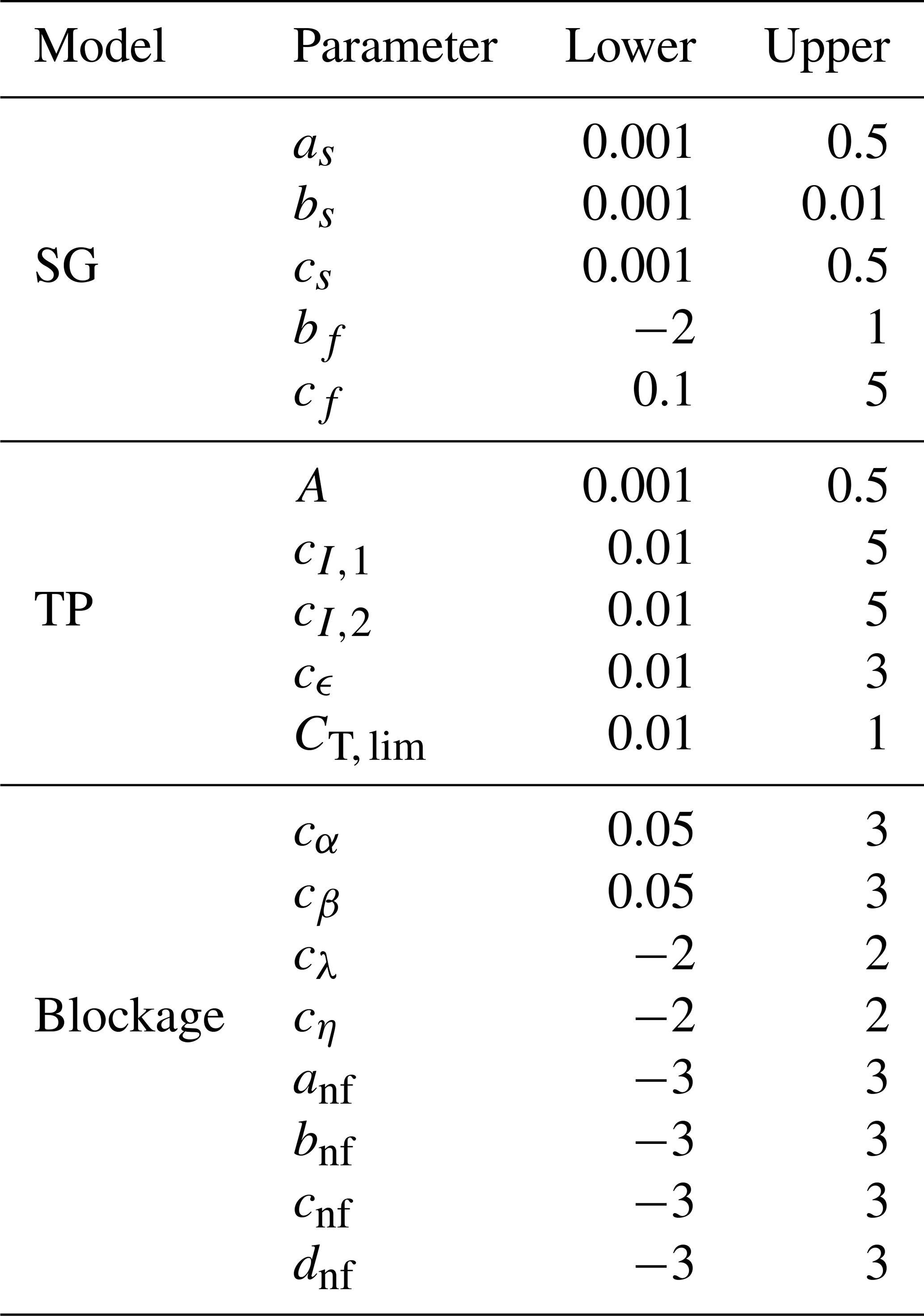
The Bayesian optimization framework proposed by Nogueira (2014) is used to minimize the L² norm between the hub-height velocity fields of the RANS data and the deficit models. For each flow case, an L² norm is calculated, and the mean of those is used as the optimization objective function. The deficit models are calibrated to account for velocities between 2–10 rotor diameters downstream of the source turbine and up to 2 rotor diameters in the cross-flow direction. The upstream deficit model is calibrated considering the region between 1–2 rotor diameters upstream of the source turbine and up to 2 rotor diameters away in the cross-flow direction. The optimization is initialized with 50 parameter configurations sampled from uniform distributions (detailed in Table 3). A set of parameters is denoted in vector form as ϕ_i and a collection of them in matrix notation as Φ. A given set of parameters constitutes a realization of the wake deficit parameters shown in Table 3; the original parameters are not shown here but are included inside the results section with the recalibrated parameters in Table 7.

Table 3 Parameter bounds for the considered wake models during the calibration process: the SG model (Blondel and Cathelain, 2020), the TurbOPark-based model (TP; Nygaard et al., 2022), and the blockage model (Forsting et al., 2023).

This implementation of Bayesian optimization uses Gaussian process (GP) regression. Here, the posterior predictive distribution for a test input ϕ_* is given by

$$\begin{array}{}\text{(6a)}& {\displaystyle }& {\displaystyle }f\left({\mathit{\varphi }}_{*}\right)\mid \mathbf{\Phi },\mathit{y}\sim \mathcal{N}\left({\mathit{\mu }}_{\text{GP}}\left({\mathit{\varphi }}_{*}\right),{\mathit{\sigma }}_{\text{GP}}^{\mathrm{2}}\left({\mathit{\varphi }}_{*}\right)\right),\text{(6b)}& {\displaystyle }& {\displaystyle }{\mathit{\mu }}_{\text{GP}}\left({\mathit{\varphi }}_{*}\right)={\mathit{k}}_{*}^{\top }{\left(\mathbf{K}+{\mathit{\sigma }}_n^{\mathrm{2}}{\mathbb{I}}_n\right)}^{-\mathrm{1}}\mathit{y},\text{(6c)}& {\displaystyle }& {\displaystyle }{\mathit{\sigma }}_{\text{GP}}^{\mathrm{2}}\left({\mathit{\varphi }}_{*}\right)=k({\mathit{\varphi }}_{*},{\mathit{\varphi }}_{*})-{\mathit{k}}_{*}^{\top }{\left(\mathbf{K}+{\mathit{\sigma }}_n^{\mathrm{2}}{\mathbb{I}}_n\right)}^{-\mathrm{1}}{\mathit{k}}_{*},\end{array}$$

where 𝒩(μ,σ²) denotes a Gaussian distribution with mean μ and SD σ, y is the vector of observed outputs at the n training points, σ_n can be used to account for observation and model uncertainty but is just included here for numerical stability with ${\mathit{\sigma }}_n={\mathrm{10}}^{-\mathrm{3}}$, 𝕀_n is the n×n identity matrix, and μ_GP and σ_GP are the mean and SD obtained through GP regression. The covariance matrix K and test covariance vector k_* are constructed using a pre-specified kernel function. This framework uses a Matérn kernel for the GP regressor with smoothness parameter ν_M=2.5 and length scale set to 1, which can therefore be removed as it only occurs in denominators; the Matérn kernel is shown in Eq. (7).

$$\begin{array}{ll}{\displaystyle }& {\displaystyle }k({\mathit{\varphi }}_i,{\mathit{\varphi }}_j)={\displaystyle \frac{\mathrm{1}}{\mathrm{\Gamma }\left({\mathit{\nu }}_{\mathrm{M}}\right){\mathrm{2}}^{{\mathit{\nu }}_{\mathrm{M}}-\mathrm{1}}}}{\left(\sqrt{\mathrm{2}{\mathit{\nu }}_{\mathrm{M}}}\Vert {\mathit{\varphi }}_i-{\mathit{\varphi }}_j{\Vert }_{\mathrm{2}}\right)}^{{\mathit{\nu }}_{\mathrm{M}}}\\ \text{(7)}& {\displaystyle }& {\displaystyle }\times K_{{\mathit{\nu }}_{\mathrm{M}}}\left(\sqrt{\mathrm{2}{\mathit{\nu }}_{\mathrm{M}}}\Vert {\mathit{\varphi }}_i-{\mathit{\varphi }}_j{\Vert }_{\mathrm{2}}\right)\end{array}$$

Here k(ϕ_i,ϕ_j) is the Matérn covariance between parameter sets ϕ_i and ϕ_j, $K_{{\mathit{\nu }}_{\mathrm{M}}}$ is the modified Bessel function of the second kind, and Γ is the gamma function. The elements of the covariance matrix K are given by $K_{ij}=k({\mathit{\varphi }}_i,{\mathit{\varphi }}_j)$, and the test vector is

$$\begin{array}{}\text{(8)}& {\displaystyle }{\displaystyle }{\mathit{k}}_{*}={\left[\begin{array}{cccc}k({\mathit{\varphi }}_{\mathrm{1}},{\mathit{\varphi }}_{*})& k({\mathit{\varphi }}_{\mathrm{2}},{\mathit{\varphi }}_{*})& \mathrm{\cdots }& k({\mathit{\varphi }}_n,{\mathit{\varphi }}_{*})\end{array}\right]}^{\top }.\end{array}$$

To guide the selection of the next evaluation point, an acquisition function is required. This implementation uses the upper confidence bound (UCB) acquisition function to decide the next best set of parameters. In this implementation, an exploration parameter of κ=2.576 is used for UCB, as shown in Eq. (9).

$$\begin{array}{}\text{(9)}& {\displaystyle }{\displaystyle }\text{UCB}\left({\mathit{\varphi }}_{*}\right)=g\left(f\left({\mathit{\varphi }}_{*}\right)\mid \mathbf{\Phi },\mathit{y}\right)={\mathit{\mu }}_{\text{GP}}\left({\mathit{\varphi }}_{*}\right)+\mathit{\kappa }{\mathit{\sigma }}_{\text{GP}}\left({\mathit{\varphi }}_{*}\right)\end{array}$$

The Bayesian optimization is run for 200 sequential iterations. In each iteration, the GP model is fitted to all previously observed parameter sets, the UCB acquisition function is maximized to select the following parameter set ϕ_* to evaluate, and the objective function is computed at this point. After all iterations, the parameters associated with the lowest error are reported.

2.4 Artificial neural network (ANN) surrogate

In this work, a pre-trained RANS-based wake surrogate developed by Pish et al. (2024), based on the work of Schøler et al. (2023), is employed for wind farm simulations and WFLO. The surrogate is based on a conventional ANN architecture, commonly referred to as a deep neural network, a fully connected feed-forward neural network, or a multi-layer perceptron (MLP). The model takes the Cartesian position in space (x, y, z), the yaw offset from the inflow direction (γ), C_T, and the TI as inputs. While TI is considered during our experiments, yaw misalignment is not. Not addressing yaw misalignment was a conscious decision to limit the scope of the paper as it would have entailed a significant increase in the number of cases to evaluate with RANS.

Table 4 Architecture of the pre-trained RANS ANN surrogates for the velocity deficit (Δu) and added-turbulence (I_a) outputs.

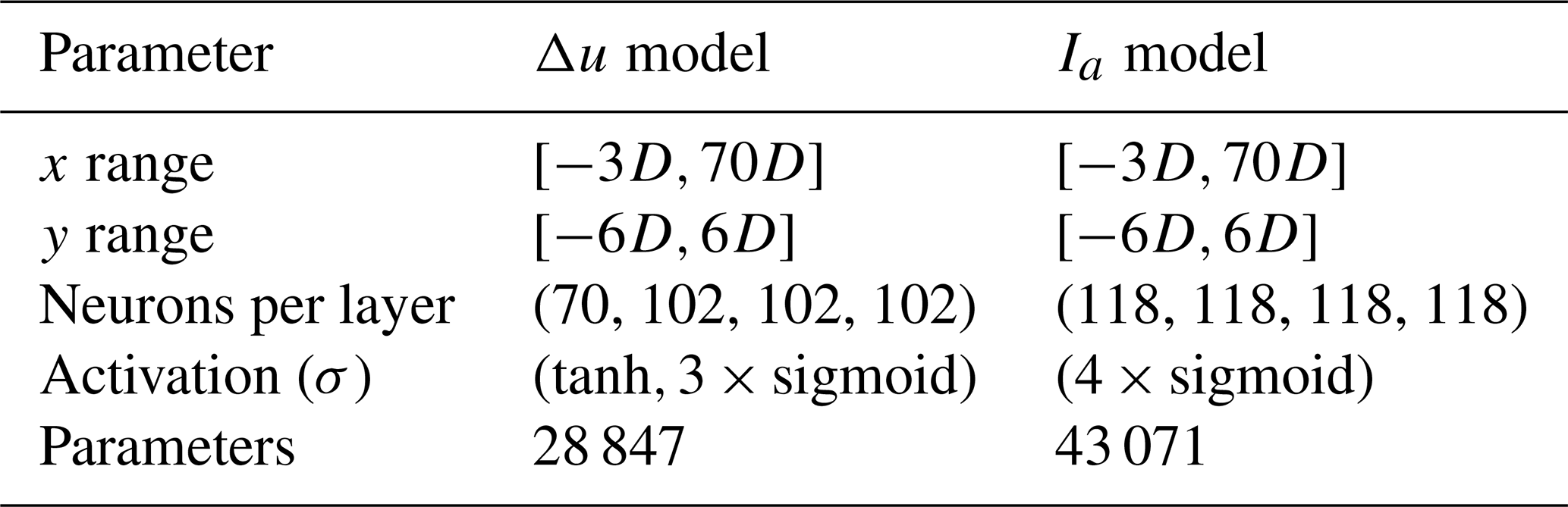
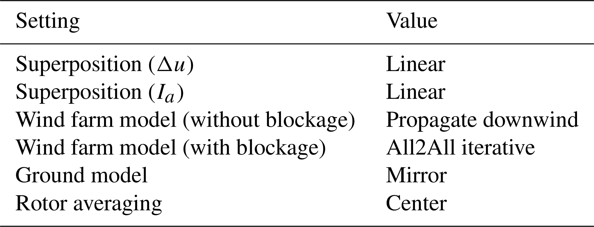
Table 5 Configuration used to deploy the ANN surrogates as wake models in PyWake.

In Eq. (10) the MLP is defined as a set of equations. Equation (10a) shows the input s, Eq. (10b) shows the hidden layer l, and Eq. (10c) shows the output of the MLP f_θ(s).

$$\begin{array}{}\text{(10a)}& {\displaystyle }& {\displaystyle }{\mathit{h}}^{\left(\mathrm{0}\right)}=\mathit{s}={\left[\begin{array}{cccccc}x,& y,& z,& \mathit{\gamma },& C_{\mathrm{T}},& I\end{array}\right]}^{\top }\text{(10b)}& {\displaystyle }& {\displaystyle }{\mathit{h}}^{\left(l\right)}={\mathit{\sigma }}^{\left(l\right)}\left({\mathbf{W}}^{\left(l\right)}{\mathit{h}}^{(l-\mathrm{1})}+{\mathit{b}}^{\left(l\right)}\right),l=\mathrm{1},\mathrm{2},\mathrm{\dots },L-\mathrm{1}\text{(10c)}& {\displaystyle }& {\displaystyle }{\mathit{f}}_{\mathit{\theta }}\left(\mathit{s}\right)={\mathbf{W}}^{\left(L\right)}{\mathit{h}}^{(L-\mathrm{1})}+{\mathit{b}}^{\left(L\right)}\end{array}$$

Here h^(l), σ^(l), W^(l), and b^(l) are the activation, activation function, weights, and bias at layer l, respectively, and L is the total number of layers. The model is trained with a single-wake RANS dataset of the DTU 10 MW reference wind turbine (Bak et al., 2013). The architectures of the employed models are summarized in Table 4, and a brief overview of the engineering model configuration for the ANN is presented in Table 5. The configuration was adopted in accordance with Pish et al. (2024).

2.5 Wind farm flow study

To evaluate the accuracy of the three low-fidelity options – the two engineering models and the ANN surrogate – we conduct a systematic study examining the influence of turbine count and inter-turbine spacing. Because flow construction based on superposition inherently introduces errors that depend on these parameters, varying them enables a structured investigation of construction error and facilitates a direct comparison of the engineering models and the ANN. Additionally, the study examines how these factors impact memory requirements and computational costs.

To examine the effect of turbine count, six base layouts are considered with $n_{\text{wt}}\in \mathit{\{}\mathrm{6},\mathrm{10},\mathrm{20},\mathrm{30},\mathrm{40},\mathrm{50}\mathit{\}}$. Figure 3 illustrates these configurations. To assess the impact of inter-turbine spacing, each base layout is scaled by a separation factor $s_{\text{wf}}\in \mathit{\{}\mathrm{3}D,\mathrm{5}D,\mathrm{7}D\mathit{\}}$, resulting in a total of 18 distinct layouts. Each layout is simulated using RANS, the recalibrated and original engineering models, and the ANN surrogate. By comparing these results, trends in model performance can be identified, and the effectiveness of the ANN surrogate can be evaluated.

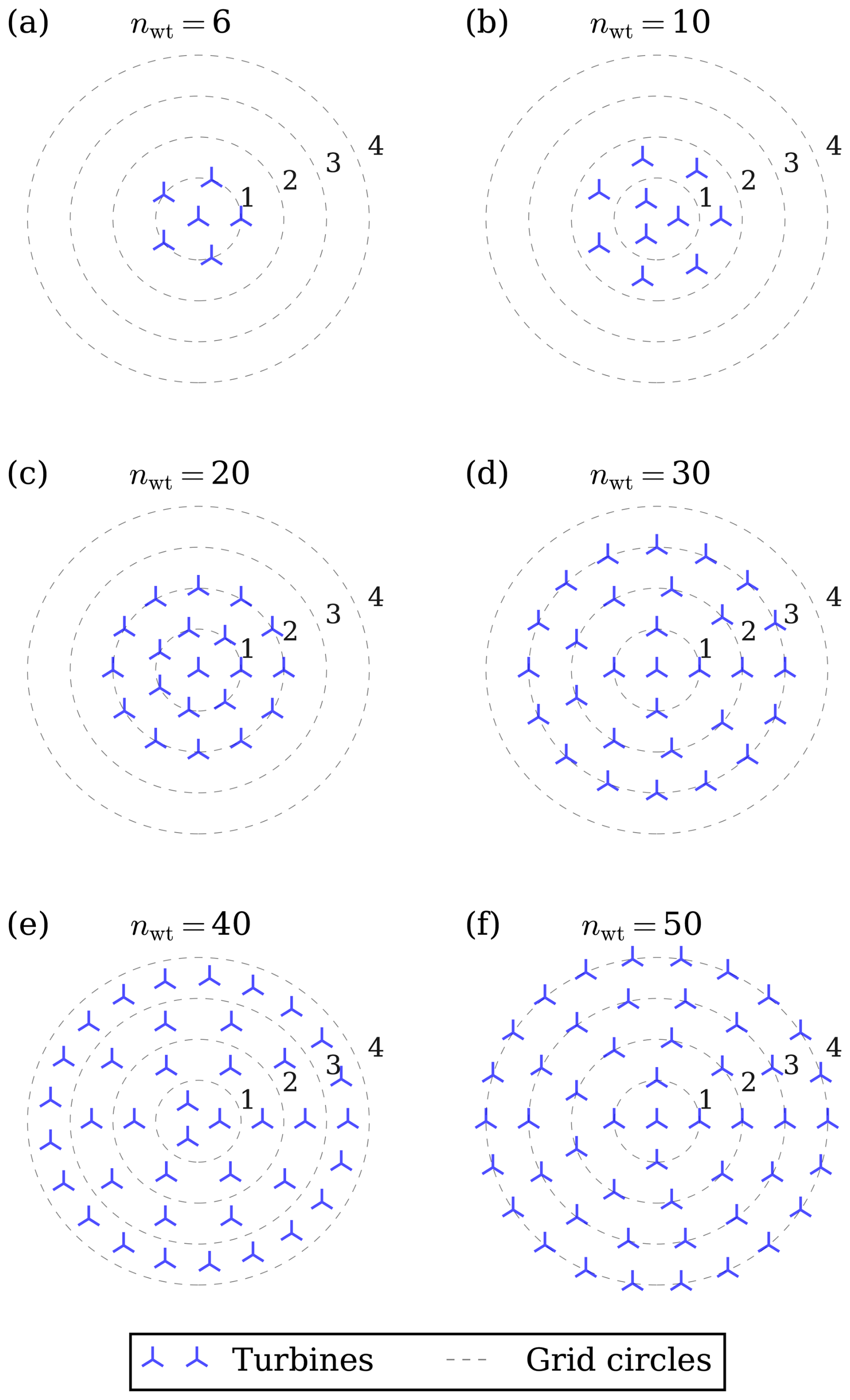
Figure 3 Circular turbine layouts evaluated in the wind farm flow study. The grid circles represent normalized radial positions, which are scaled by a separation factor $s_{\text{wf}}\in \mathit{\{}\mathrm{3}D,\mathrm{5}D,\mathrm{7}D\mathit{\}}$ to generate configurations with varying inter-turbine spacing.

In the flow study, each possible model-layout combination is evaluated under different inflow conditions consisting of wind speeds $U=\mathrm{8.0}\mathrm{m}{\mathrm{s}}^{-\mathrm{1}}$ and 14 m s⁻¹, ambient turbulence intensities I=5 % and 10 %, and wind direction angles θ ranging from 270 to 315° in increments of 3°.

2.6 Wind farm layout optimization (WFLO)

To compare the low-fidelity models in WFLO, optimization is performed using each of the available low-fidelity models, and the results are validated by estimating the annual energy production (AEP) with RANS simulation. A WFLO case is formulated with the objective of maximizing AEP, subject to a minimum turbine separation s_min=2D and polygonal boundary 𝒫:

$$\begin{array}{ll}{\displaystyle }& {\displaystyle }\underset{\mathit{\left\{}\right(x_i,y_i){\mathit{\}}}_{i=\mathrm{1}}^{n_{\text{wt}}}}{max}\text{AEP}\left(\mathit{\left\{}\right(x_i,y_i){\mathit{\}}}_{i=\mathrm{1}}^{n_{\text{wt}}}\right)\\ {\displaystyle }& {\displaystyle }\approx \mathrm{8760}\sum _{i=\mathrm{1}}^{n_{\text{wt}}}\sum _{j=\mathrm{1}}^{n_{\mathcal{U}}}\sum _{k=\mathrm{1}}^{n_{\mathit{\theta }}}{P}_i\left(\mathit{\right\{}(x_m,y_m){\mathit{\}}}_{m=\mathrm{1}}^{n_{\text{wt}}},{\mathcal{U}}_j,{\mathit{\theta }}_k\left)\mathit{\rho }\right({\mathcal{U}}_j,{\mathit{\theta }}_k)\\ {\displaystyle }& {\displaystyle }\text{s.t. }\sqrt{(x_i-x_q{)}^{\mathrm{2}}+(y_i-y_q{)}^{\mathrm{2}}}\ge s_{min},\forall i\ne q\\ \text{(11)}& {\displaystyle }& {\displaystyle }(x_i,y_i)\in \mathcal{P},\forall i=\mathrm{1},\mathrm{\dots },n_{\text{wt}},\end{array}$$

where x_i, y_i, and P_i are coordinates and power produced at turbine i, 8760 is the number of hours in a year, and n_wt is the number of turbines. ρ is a probability mass function indicating the probability of seeing a given combination of wind speed bin 𝒰_j and binned wind direction θ_k. During optimization, the AEP is estimated with a wind direction bin for every 1° to avoid artificially unwaked areas which the optimization algorithms would exploit. However, during validation the bin discretization was decreased to only consider a bin for every 5° to conserve computational resources driven by the cost of RANS simulations, as discussed in Sect. 2.1.

Table 6 Parameters of considered optimization algorithms as used during studies with TopFarm2.

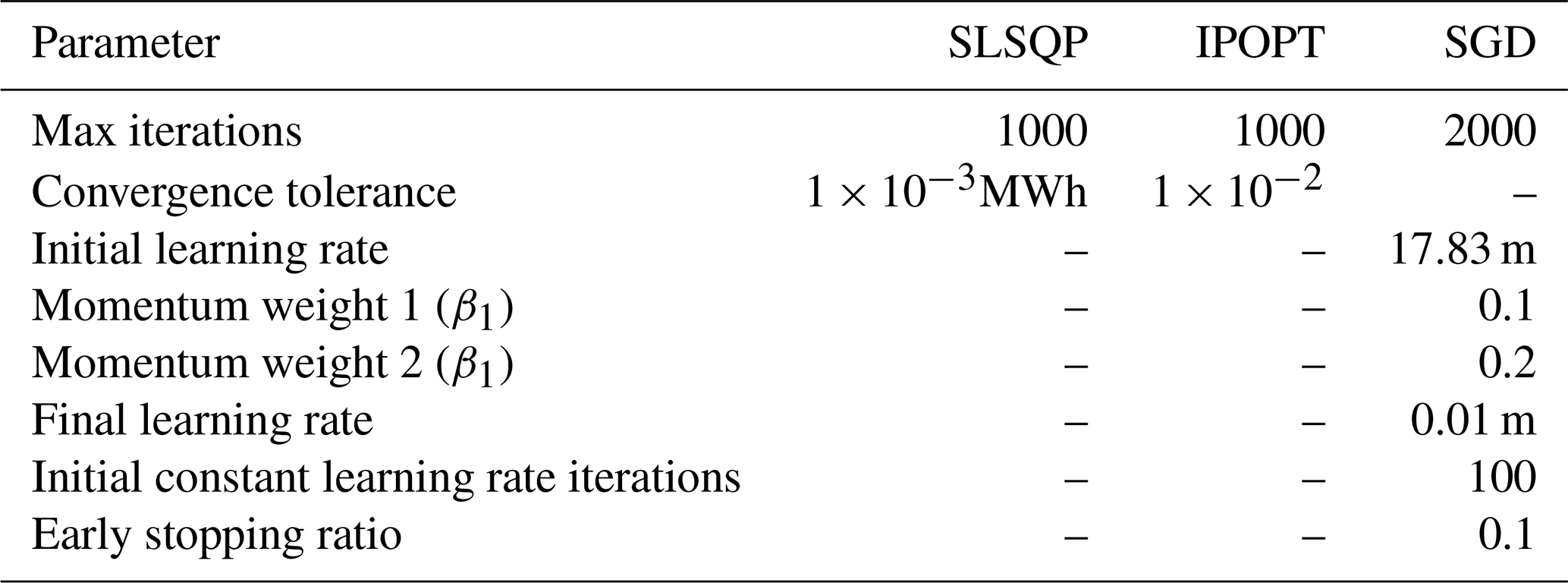
The optimization is performed with the DTU-developed software Topfarm2 (Pedersen et al., 2025). Three different gradient-based optimization algorithms are considered, as implemented in Topfarm2: sequential least squares quadratic programming (SLSQP) (Kraft, 1988; Virtanen et al., 2020), interior point optimizer (IPOPT) (Wächter and Biegler, 2006), and stochastic gradient descent (SGD) (Quick et al., 2023). In all cases, the gradients for the optimization are provided by the automatic differentiation included in PyWake.

The wind climate used in the layout study is taken from the IEA Wind 740-10-MW reference offshore wind plant (Kainz et al., 2024): the wind rose in Fig. 4b is adopted as the site inflow distribution. The boundary was designed for this study to accommodate many turbines inside a small area, while maintaining both sharp and soft edges. The RANS cost scales with the modeled area because the wind directions are modeled by rotating the farm. A circular boundary minimizes this area and is shown here as the smallest circle enclosing the farm (radius R_wf in Fig. 4a). The turbines are modeled as the DTU 10 MW reference wind turbine (Bak et al., 2013). The initial and optimized coordinates for the best optimization runs are shown in Appendix B. To simplify both optimization and validation, the ambient TI was set to I₀=6 % for all flow cases. The layout optimization procedure is performed for each low-fidelity model, both with and without a blockage model, and for the engineering models in their original and recalibrated forms, using multiple optimization algorithms and random initial layouts. For cases without blockage, all three optimization algorithms, SLSQP, IPOPT, and SGD, are used, each initialized from the same set of five randomly generated layouts to enable a consistent comparison across algorithms.

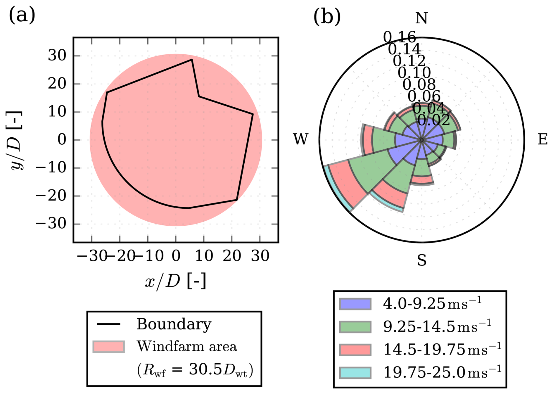
Figure 4 (a) Boundary constraint for the considered layout optimization. (b) Wind rose at the considered IEA 740-10-MW reference site.

For cases including the blockage model, 10 random initial layouts are considered; however, only the SGD algorithm is used, as it is less memory-intensive than the other approaches due to batch sampling of the wind rose. From the resulting set of optimized layouts, the layout yielding the highest AEP is selected for each low-fidelity model and subsequently validated using RANS simulations, thereby limiting the total number of RANS cases to one per low-fidelity model.

2.7 Evaluation metrics

To evaluate the relative performance of the different models, quantitative measures are needed. In this work, we use the mean absolute percentage error (MAPE), the root mean square error (RMSE), the maximum absolute error (E_max), and the error standard deviation (σ_E).

$$\begin{array}{}\text{(12a)}& {\displaystyle }& {\displaystyle }\text{MAPE}={\displaystyle \frac{\mathrm{1}}{N}}\sum _{i=\mathrm{1}}^N\left|{\displaystyle \frac{u_i-u_i^{\prime }}{U_i}}\right|\cdot \mathrm{100}\text{(12b)}& {\displaystyle }& {\displaystyle }\text{RMSE}=\sqrt{{\displaystyle \frac{\mathrm{1}}{N}}\sum _{i=\mathrm{1}}^N{\left(u_i-u_i^{\prime }\right)}^{\mathrm{2}}}\text{(12c)}& {\displaystyle }& {\displaystyle }{E}_{\text{max}}=\underset{i}{max}|u_i-u_i^{\prime }|\text{(12d)}& {\displaystyle }& {\displaystyle }{\mathit{\sigma }}_E=\sqrt{{\displaystyle \frac{\mathrm{1}}{N-\mathrm{1}}}\sum _{i=\mathrm{1}}^N{\left((u_i-u_i^{\prime })-{\displaystyle \frac{\mathrm{1}}{N}}\sum _{j=\mathrm{1}}^N(u_j-u_j^{\prime })\right)}^{\mathrm{2}}}\end{array}$$

Here u_i is the target wind speed for observation i, $u_i^{\prime }$ is the predicted wind speed, and N is the total number of observations. In Eq. (12a) the denominator uses the free-stream velocity U_i rather than u_i, in order to avoid numerical issues in heavily waked regions, where low wind speeds can lead to disproportionately large relative errors. Conversely, this formulation prevents large errors in unwaked regions from being underrepresented in the overall metric.

For flow field comparisons, regions within 1 rotor diameter of the turbines are omitted, making the analysis domain (Ω) a subset of the whole flow domain (Ω_flow). The whole flow domain is the hub-height flow plane, with grid parameters provided in Table 1 and shown in Fig. 2.

$$\begin{array}{ll}{\displaystyle }& {\displaystyle }\mathrm{\Omega }=\mathit{\left\{}\right(x,y)\in {\mathrm{\Omega }}_{\text{flow}}|\sqrt{(x-x_i{)}^{\mathrm{2}}+(y-y_i{)}^{\mathrm{2}}}\ge D\\ \text{(13)}& {\displaystyle }& {\displaystyle }\forall i=\mathrm{1},\mathrm{2},\mathrm{\dots },n_{\text{wt}}\mathit{\}}\end{array}$$

Where this subset is used, the metric will be marked with an Ω subscript.

3 Results and discussion

This section presents and discusses the results of the three studies introduced in Sect. 2. First, the recalibration of the two engineering models against the RANS single-wake dataset is reported. Next, the wind farm flow study compares the ANN surrogate and both the recalibrated and the originally calibrated engineering models against RANS across varying turbine counts and inter-turbine spacings and assesses their computational cost and memory requirements. Finally, the WFLO study validates optimized layouts obtained with each of the low-fidelity models against RANS-based AEP calculations.

3.1 Recalibration of wake models with RANS data

The recalibrated model parameters are summarized in Table 7, where the original parameter values are also included. Overall, the changes are not dramatic: the sign of each parameter is preserved. However, several parameters do show substantial numerical differences.

(Blondel and Cathelain, 2020)(Nygaard et al., 2022)(Forsting et al., 2023)

Table 7 Original and recalibrated parameters for the considered wake and blockage models.

(Blondel and Cathelain, 2020)(Nygaard et al., 2022)(Forsting et al., 2023)

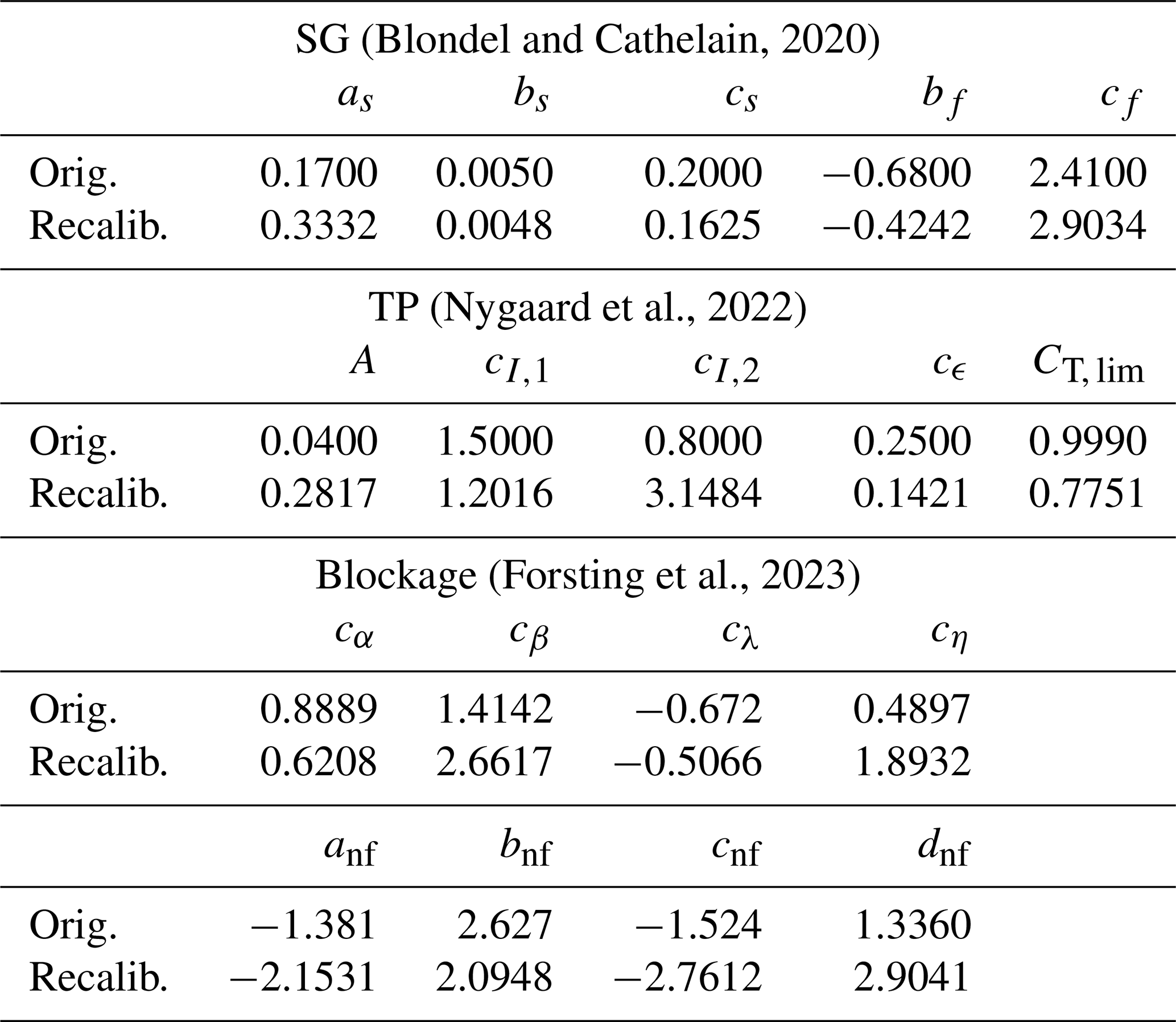
Table 8 Metrics before and after recalibration for the two considered models.

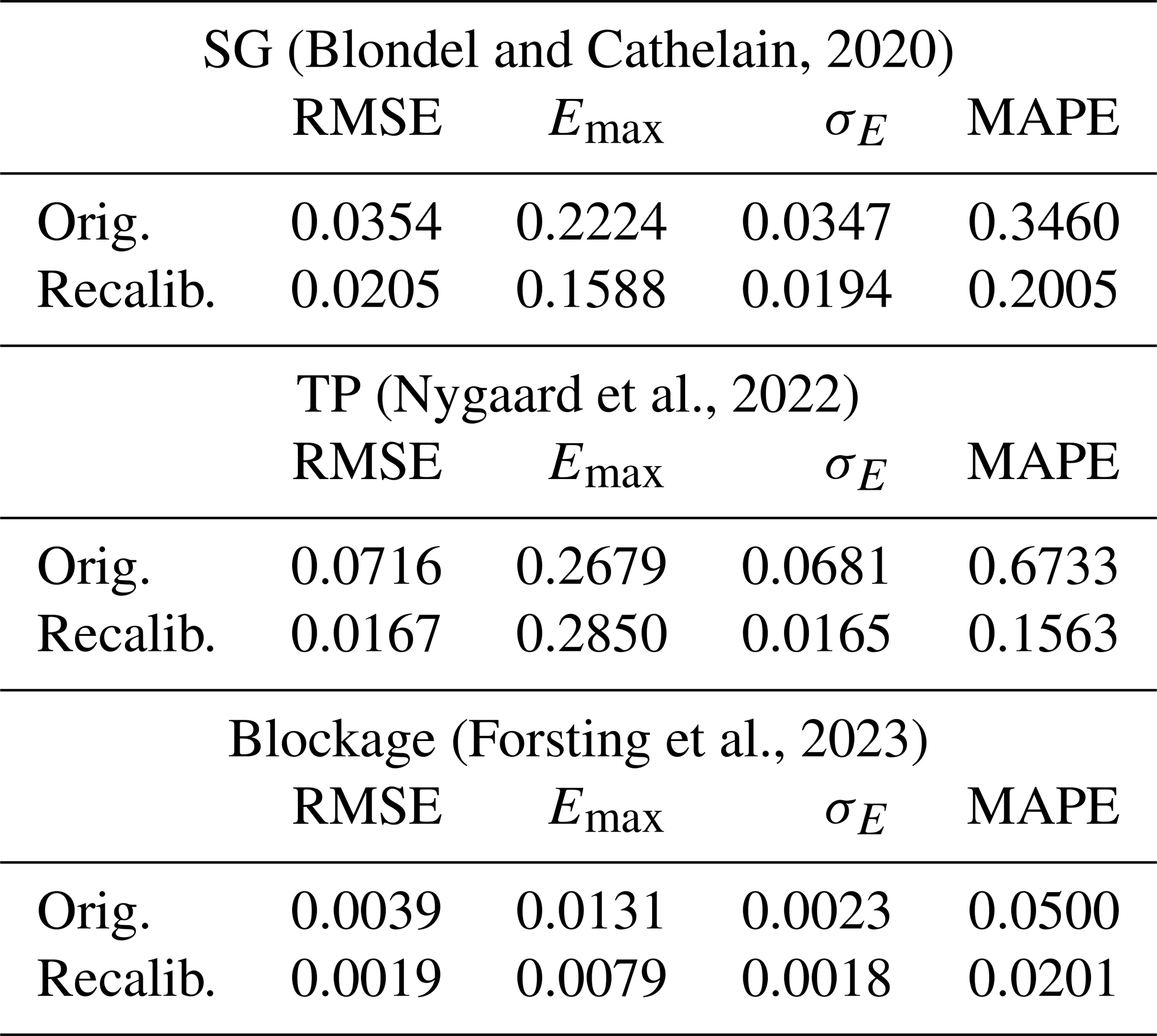
For the SG model, most changes are relatively small, except for a_s, which increases from 0.17 to 0.33. This parameter governs the relationship between wake width and rotor thrust. Because the original calibration was based on a mix of experimental data, whereas the present work uses RANS data, different thrust and wake-width characteristics are expected; therefore, a noticeable change in a_s is expected.

For the TP model, the parameter c_I,2 changes markedly from 0.80 to approximately 3.15. The parameters c_I,1 and c_I,2 impact the auxiliary variables α and β in Nygaard et al. (2022), which together act as replacements for both the ambient TI and C_T in the wake expansion formulation. The initial values for c_I,1 and c_I,2 were used from Frandsen (2005) and the IEC (2010). The original value was derived from measurement data, whereas the present RANS simulations employ a fundamentally different turbulence formulation. Consequently, a substantial adjustment is required for consistency with the RANS flow. Note that the recalibrated C_T, lim of the TP model lies below the maximum C_T of the DTU 10 MW thrust curve (0.9), so it acts as an active wake-shaping parameter at high thrust rather than only as a C_T≥1 safeguard. The SG model lacks an equivalent parameter, so the two configurations were not calibrated on a fully symmetric parameter set. Future comparisons should be mindful of this difference and treat the clip consistently across models. Furthermore, a lower value of both c_ϵ and C_T, lim makes the initial wake narrower for high C_T values above the limit. This tends to compensate for the higher A value, which leads to greater wake spreading.

In the self-similarity deficit blockage model, the polynomial-fit parameters a_nf, b_nf, c_nf, and d_nf also vary considerably. Because these coefficients describe a polynomial rather than a directly interpretable physical relationship, the practical implications of their changes are difficult to interpret. The parameters c_β and c_λ, however, are more interpretable and show meaningful shifts. The parameter c_λ represents an offset in the linear rotor half-radius induction zone, introduced to correct for wind farm blockage effects – effects that are absent in the single-turbine RANS dataset used here. A significant change is therefore expected. The scaling factor c_β, which modulates the influence of the rotor half radius, is similarly affected.

In Table 8, error metrics are collected to compare results before and after recalibration. The error metrics in Table 8 show improvements across all measures for the SG and blockage models. For the TP model, most metrics also improve, except for the maximum absolute error. This exception was surprising, but as the remaining metrics improved, it is expected that this was due to a large error near the rotor, where the self-similar far-wake assumption underlying the Gaussian deficit does not yet hold (Blondel and Cathelain, 2020). This idea is supported by inspecting the spatial distribution of the mean RMSE (averaged over inflow conditions) in Fig. 5d, which indicates that the most significant errors occur immediately behind the turbine at x=2D.

Figure 5 Wake and blockage model calibration RMSE error maps.

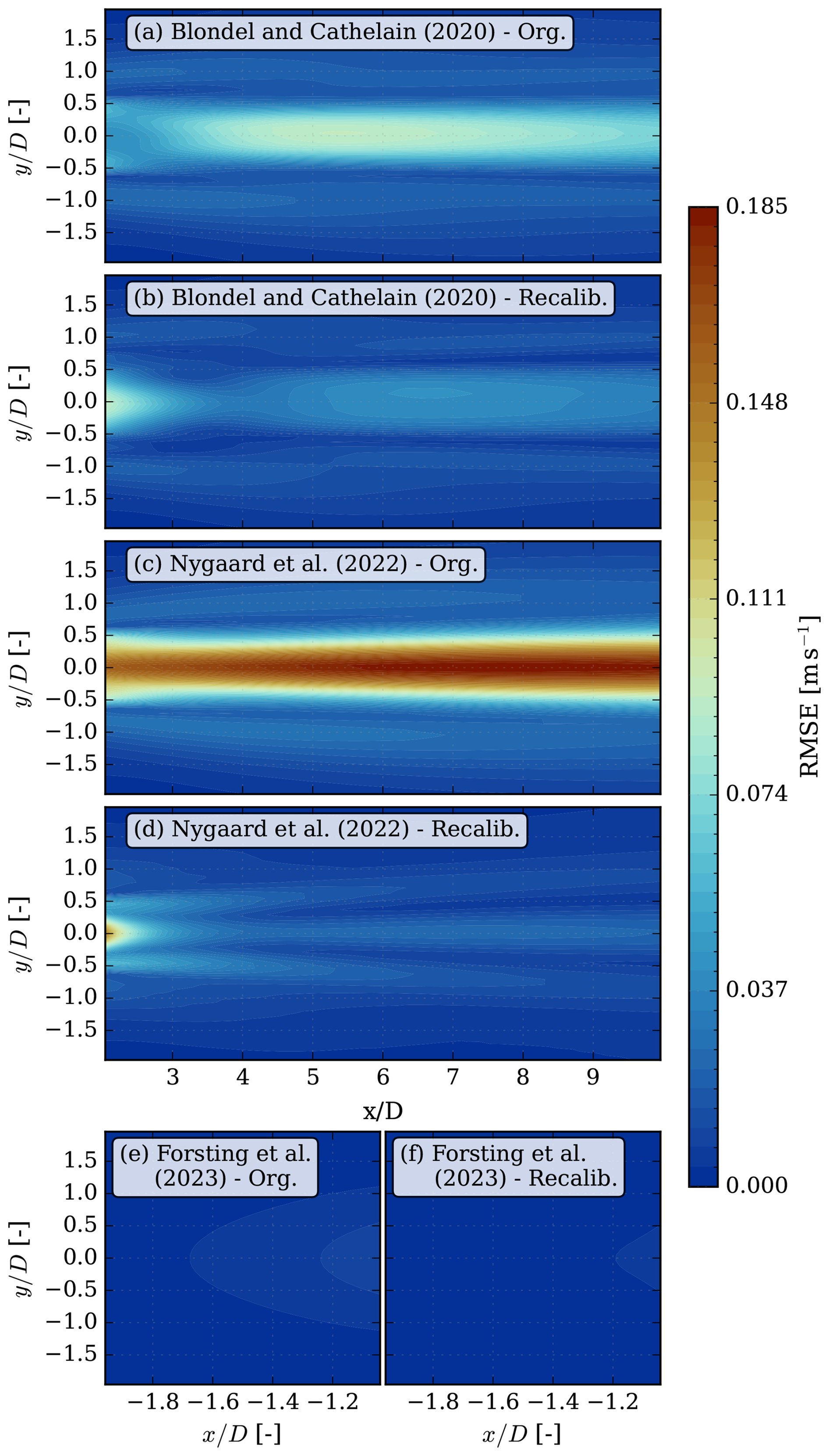
The overall takeaway from Fig. 5 is that the recalibrated models yield substantially improved performance, particularly outside the near wake. The TP model exhibits the greatest overall improvement, which aligns with expectations: the original TurbOPark model of Nygaard et al. (2020) was calibrated against wind farm flow data, encompassing both intra-farm and inter-farm wake interactions rather than isolated single wakes, and therefore requires the largest recalibration to perform well in the single-wake context evaluated here. By contrast, the original super-Gaussian model by Blondel and Cathelain (2020) was calibrated on single-wake data and requires comparatively little correction in this setting.

3.2 Wind farm flow study

The layouts introduced in Fig. 3 were evaluated with separation factors $s_{\text{wf}}\in \mathit{\{}\mathrm{3}D,\mathrm{5}D,\mathrm{7}D\mathit{\}}$. Flow simulations were performed using all the available low-fidelity models (SG model, TP model, and the ANN), with the engineering models assessed in both recalibrated and original forms. To distinguish the recalibrated models from the original models, a superscript (^†) is used with the original models; e.g., SG^† refers to the SG model with original parameters. Similarly, to distinguish between the models with and without blockage, a superscript (^*) is used to indicate the inclusion of blockage; e.g., SG${}^{†*}$ indicates the original SG model with blockage.

To quantify the accuracy of the lower-fidelity simulations, the RANS simulations described in Sect. 2.1 were used as the reference ground truth. A masked flow domain, defined in Eq. (13), was applied to exclude the region immediately surrounding each turbine, as this region is irrelevant for optimization and does not represent a feasible turbine spacing. Figure 6 presents MAPE_Ω and RMSE_Ω as functions of the number of turbines n_wt, with mean values indicated by solid lines and bootstrapped 95 % confidence intervals shown as shaded regions. The ensemble mean is constructed from the considered inflow conditions, including wind directions, wind speeds, and ambient TIs.

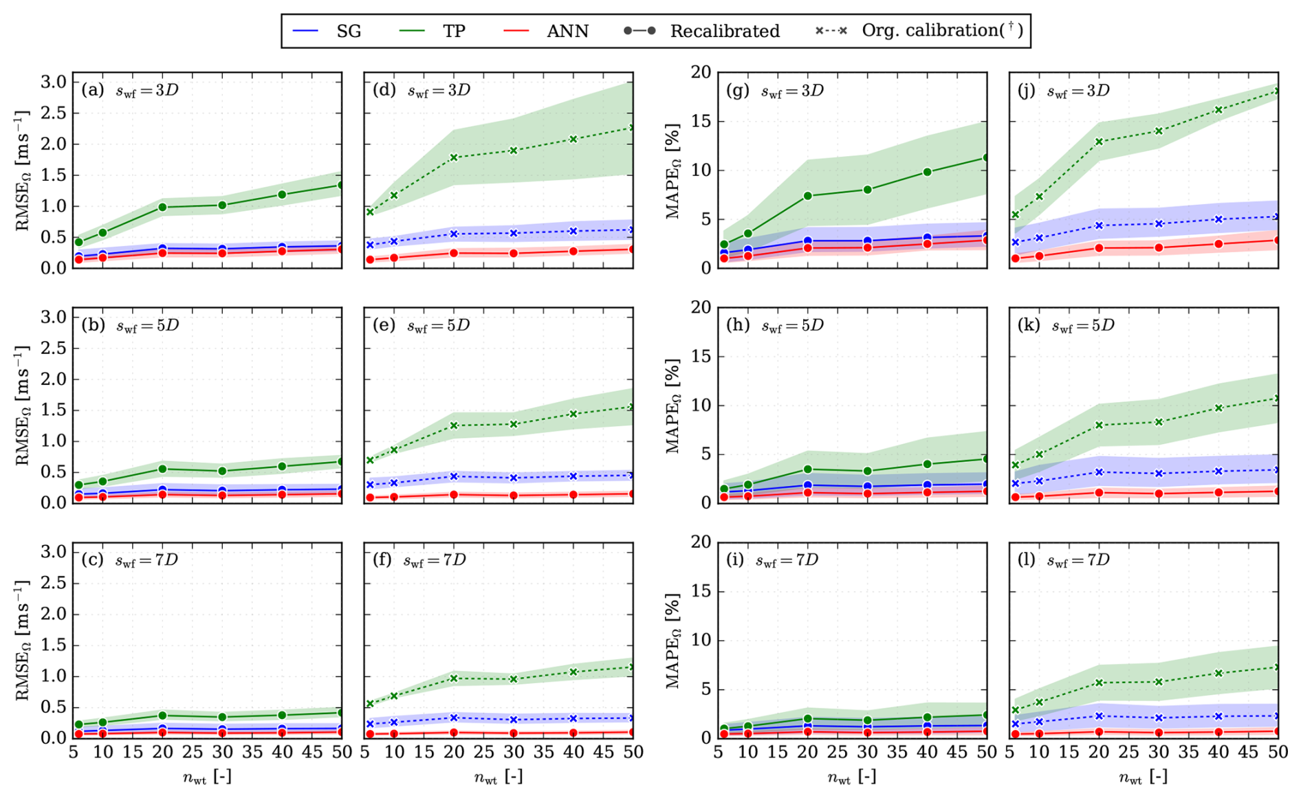
Figure 6 Flow study result metrics for an increasing number of wind turbines, without a blockage model. (a–c) RMSE_Ω with recalibrated wake models, (d–f) RMSE_Ω for the wake models with original parameters, (g–i) MAPE_Ω with recalibrated wake models, and (j–l) MAPE_Ω with wake models using the original parameters.

Figure 6 presents the results for the models without blockage; for completeness, the metrics with blockage are reported in Appendix A.

The results show that the error consistently decreases as the separation factor increases. This trend reflects the increasing complexity of the wake interactions at smaller inter-turbine distances. In these regimes, near-wake dynamics violate key assumptions in simplified wake models, particularly the superposition of individual wakes, which becomes progressively less valid as group effects strengthen (e.g., Andersen et al., 2014; Gunn et al., 2016). Simultaneously, the wake of a single turbine also behaves in a more complex manner in the near wake, further complicating the modeling of denser farms. Similarly, there is a shared trend of the error growing with the number of turbines, though at times it is subtle, which can be explained by the modeling error of superposing wakes, becoming increasingly problematic as the number of turbines increases. The trend in regard to the number of turbines is not as pronounced as for the separation factor; for interested readers, a version of Fig. 6 with a logarithmic axis is available in Appendix C. These trends between the error and the number of turbines and turbine density are observed for both the recalibrated and the original engineering models. It is also observed that the SG model with the lowest recalibration error is the one with the lowest error here, increasing confidence in the recalibration process.

Furthermore, calibration improves the engineering models across both configurations, reducing the mean error and the width of the confidence intervals, indicating improvements in accuracy and robustness across wind directions and inflow conditions. An exception occurs for the MAPE_Ω of the TP model at s_wf=3D, where calibration produces a lower mean error, but the confidence interval worsens. The reason is not immediately apparent, though it could be that the original model was intended for long-distance wakes and therefore produced consistent but poor results in the near wake, which would explain the poor performance.

Across all cases, the ANN-based surrogate outperforms the engineering models. Its superior performance is attributed to its ability to represent complex, spatially varying flow structures without relying on strong simplifying assumptions about wake behavior. This expressiveness enables the ANN to capture near-wake features with substantially higher fidelity, resulting in significantly lower errors than traditional engineering approaches.

In Fig. 7, the computational cost and memory consumption are plotted against the number of wind turbines. Figure 7a and b both show the computational cost, but in Fig. 7a the cost is expressed in CPU hours (CPUh), meaning that only models executed on the CPU can be compared directly. CPU hours are calculated by multiplying the wall time (in hours) by the number of CPU cores used during the simulation, allowing for a fair comparison. The nodes used have 32 cores. The engineering models can be run on a single core, unlike the ANN, which by default uses all available cores. Figure 7b, on the other hand, reports the real wall time in seconds, enabling direct comparison with the GPU-accelerated ANN. All simulations have been conducted on identical and exclusive nodes on the DTU cluster Sophia (Technical University of Denmark, 2019).

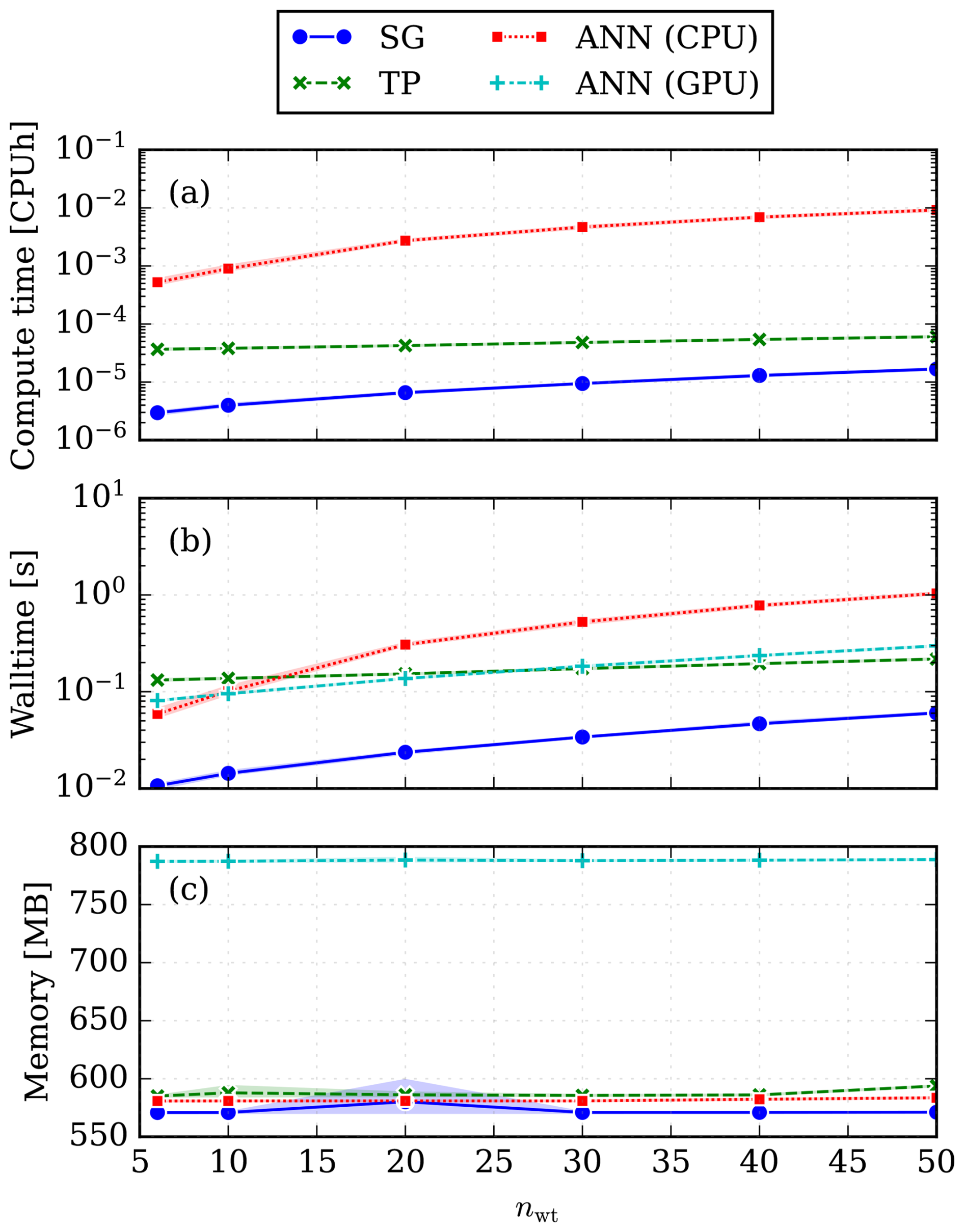
Figure 7 Average computational resource cost of a flow case for increasing wind farm sizes without inclusion of blockage. (a) Relative cost in CPU hours, (b) real-world cost in wall time (seconds), and (c) random access memory (RAM) consumption in MB.

All the results are reported with a 95 % confidence interval, based on an ensemble over the inflow conditions (wind direction, wind speed, and ambient TIs) and separation factors s_wf. The confidence is quite high, indicating that the variation in computational resource requirements with respect to layout density and inflow conditions is low. The results are shown on a semi-logarithmic plot, which likely contributes to the appearance of increasing confidence; however, it is also expected to be low.

Figure 7a shows that, in terms of CPUh, the fastest model is the SG model, followed by the TP model, with the ANN being the slowest. The ANN being the slowest is expected, as evaluating it requires multiple matrix multiplications, as described in Eq. (10), whereas the engineering models require far fewer computations. The TP model employs a Gaussian overlap for the rotor-averaging strategy, which requires additional flow evaluation and appears to increase its computational cost; however, this relative difference decreases as the number of turbines increases. In Fig. 7b, we see that the real-time performance of the ANN improves significantly when GPU acceleration is enabled, placing it roughly on par with the TP model. Without GPU acceleration, however, the computational cost of the ANN is too high for applications such as WFLO, where many repeated evaluations would otherwise become prohibitively expensive.

The memory requirements of the considered models are similar, as shown in Fig. 7c, except for the GPU-accelerated ANN, which requires more memory. However, as all models remain below 1 GB of RAM, this remains well within an acceptable range. The more pressing concern is the availability of GPU resources.

3.3 WFLO study

A series of WFLO problems was solved using the optimization algorithms listed in Table 6 for each engineering model, both recalibrated and original, as well as for the ANN model. All optimizations were executed on identical and exclusive nodes of the Sophia cluster (Technical University of Denmark, 2019) to ensure comparable runtime conditions. As PyWake at the time of writing does not support automatic GPU gradients, all optimizations have been performed using CPU resources only. Table 9 summarizes the performance of different combinations of wake models and optimization algorithms. For each algorithm within a given model, the random seed that achieved the highest expected AEP is reported. To aid interpretation, the AEP value for the best-performing algorithm in each model is highlighted in bold.

Table 9 AEP of the optimized layouts produced from the best-performing initial seeds. Results shown in bold indicate the optimization algorithm that achieved the highest AEP, selected for RANS validation.

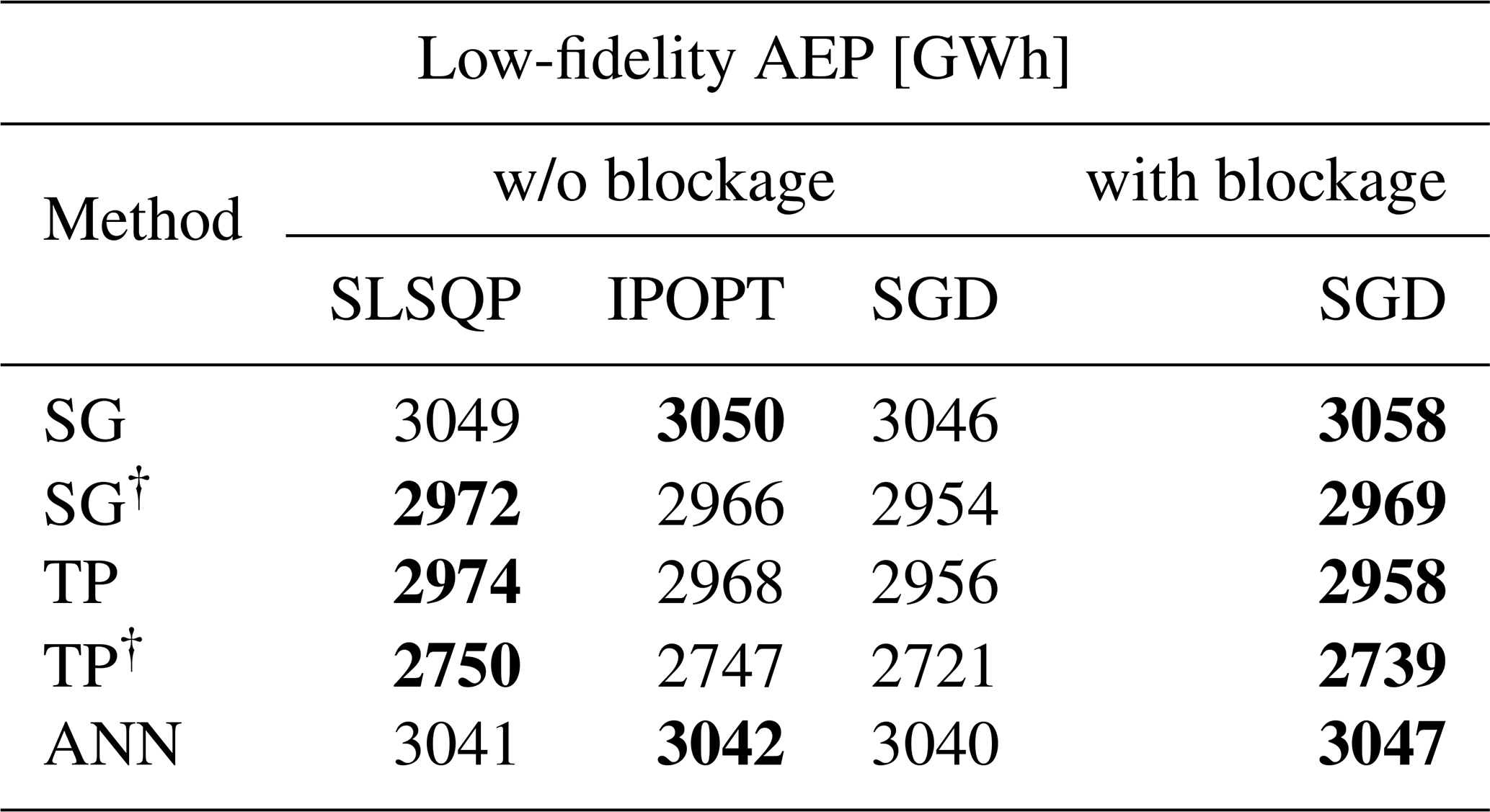
^† Model with original parameters.

The results in Table 9 are separated into cases with and without blockage. Only the SGD algorithm was used for cases with blockage due to the substantially higher memory consumption of these models. The batch sampling inherent to SGD makes it computationally less expensive, making it the only approach feasible at the required wind-rose resolution. Consequently, SGD results are used throughout for cases with blockage. A visualization of the obtained layouts is available in Appendix B.

For AEP validation with RANS, one optimized layout was selected for each low-fidelity model, both with and without blockage, corresponding to the 10 results marked with bold in Table 9. Table 10 presents the RANS AEP alongside the corresponding low-fidelity AEP and an accuracy estimate, together with key optimization metrics for assessing computational expense. The best-performing metrics in Table 10 are highlighted in bold. The inclusion of blockage did not improve the accuracy of any model, despite its greater physical fidelity; however, it substantially increased the optimization cost by factors of between $\sim \mathrm{6}\times$ and $\sim \mathrm{20}\times$. The ANN was an exception, where the blockage case was cheaper; this could be because the IPOPT algorithm, which succeeded in the case without blockage, more aggressively explores the loss landscape than the SGD, which is known to be resistant to local minima.

Table 10 Comparison of RANS-validated AEP and optimization statistics for wind farm layouts generated using different wake models, evaluated with and without blockage. The best-performing values within each category are highlighted in bold.

^† Model with original parameters. ^* Model with blockage effects included.

The TP model produced the layout with the highest RANS AEP, despite being the least accurate in predicting RANS AEP from its low-fidelity estimate, excluding models using original parameters. This outcome is somewhat unexpected given that the recalibrated models and ANN were tuned against RANS data, making RANS the designated ground-truth reference in this study. By contrast, the SG model reproduced the RANS AEP most accurately, followed closely by the ANN, with TP trailing behind significantly. Hence, the ability to reproduce the RANS AEP accurately was not correlated with the ability to find the highest RANS AEP layout through optimization in this study.

One possible explanation for this behavior is that the issue arises as an artifact of the optimization process. To investigate this, we first examine whether, among the layouts previously studied in RANS, the layout obtained using each low-fidelity model represents the best layout that the model could theoretically produce. To test this hypothesis, a cross-comparison is performed in which the AEP is calculated using each low-fidelity model for all layouts evaluated with RANS. In Fig. 8, the results of this cross-comparison are presented as a heatmap showing the change in AEP (ΔAEP) relative to the default optimized model–layout pair. Entries with positive ΔAEP in a given model row therefore indicate that a better layout exists compared to the one obtained during optimization. As illustrated in Fig. 8, significant improvements in AEP can be achieved for both the SG model and the ANN without blockage, whereas for the TP model, no better layout is available. In cases with blockage, however, there is a single better layout for the TP^* model: the one generated by the TP model without blockage. This difference is marginal and not systematic: TP^* is the only blockage case for which a better layout exists, whereas, without blockage, better layouts were available for the SG model and the ANN. As all blockage configurations use the same flow model and optimization algorithm, this isolated difference cannot be firmly attributed to any one reason, and it is suggested that further research investigate this.

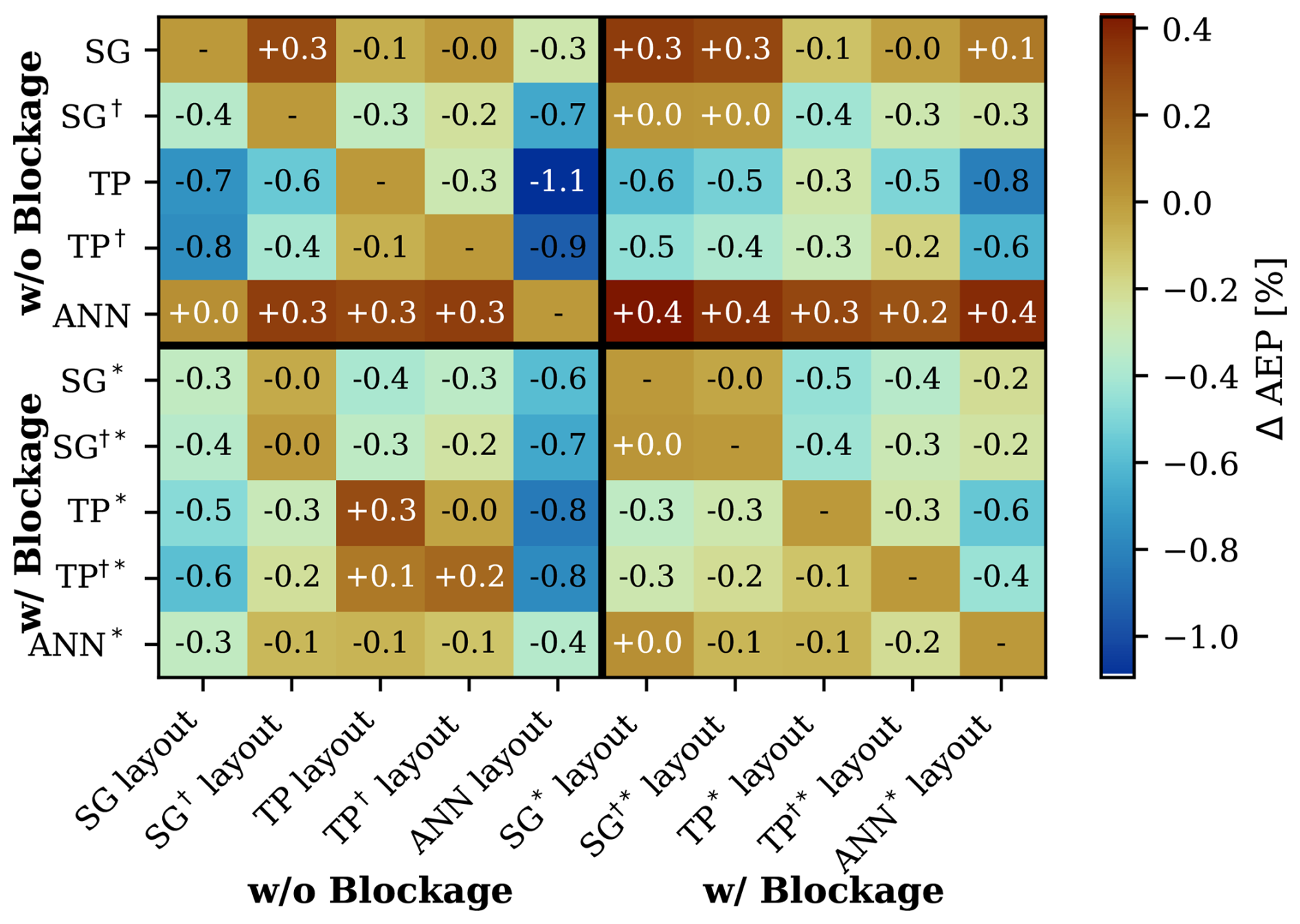
Figure 8 Cross-comparison of ΔAEP for layouts optimized by different low-fidelity models, showing changes relative to each model's default layout. Each row corresponds to a distinct model used to compute AEP. Each column corresponds to a distinct layout generated by optimizing with a selected model.

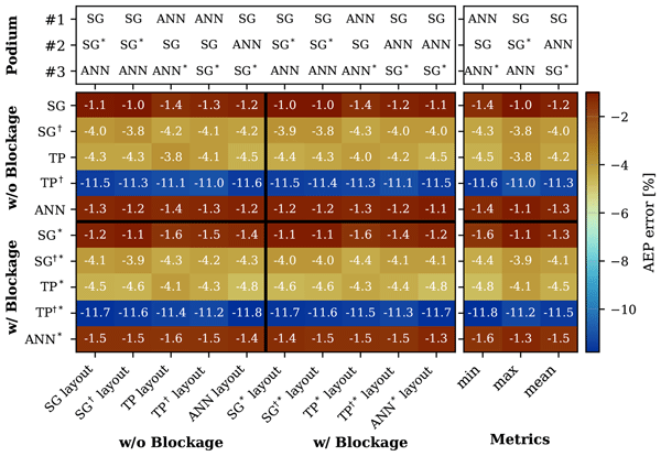
According to the data in Table 10, a trend appears indicating that the SG model and ANN produce more accurate AEP estimates than the TP model. To determine whether this trend holds more generally, the accuracy of the low-fidelity models is assessed by comparing their AEP estimates with the RANS AEP for all available layouts. This comparison is presented in Fig. 9, where additional aggregated metrics for each row have been included, along with a model podium to easily identify the models most closely matching RANS predictions for each layout. As shown in Fig. 9, the hierarchy of models in terms of AEP estimation accuracy places the TP model in third position. In contrast, the SG model and ANN compete for first place, with the SG model ultimately emerging as the most accurate. Both the SG model and the ANN are more advanced than the TP model. The SG model incorporates a transition from a top-hat shape in the near wake to a Gaussian profile in the far wake, addressing limitations of a fully Gaussian wake. In contrast, the ANN is substantially more expressive than the engineering models, with more than 28 000 tunable parameters compared to fewer than 10. While this analysis highlights differences in AEP estimation accuracy, the WFLO results reveal that accuracy alone does not guarantee optimal layouts. In fact, the recalibrated TP model produced the best layouts in our WFLO experiment, despite demonstrating the lowest accuracy among the recalibrated models.

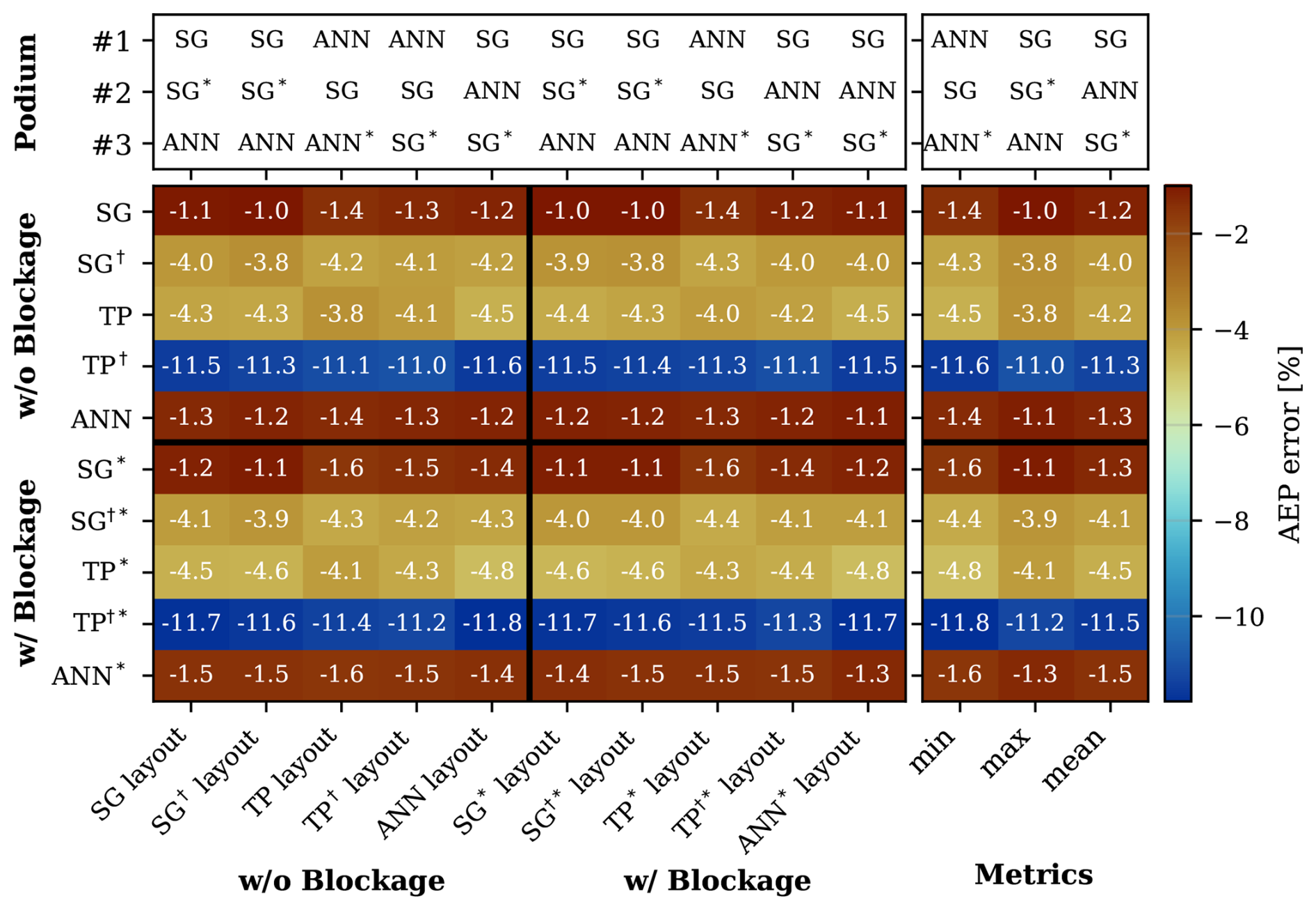
Figure 9 Comparison of AEP estimates from low-fidelity models against RANS for all layouts. Each row corresponds to a distinct model used to compute AEP. Each column corresponds to a distinct layout, which are the same layouts considered in Fig. 8. The colors show the relative difference between the RANS-computed AEP and model-computed AEP associated with each layout. Podium rows indicate the top three models that most closely matched RANS predictions for each layout, while additional columns report aggregated metrics.

The TP model achieved strong RANS AEP-validated performance despite having lower AEP accuracy than the SG and ANN models. This was the first indication we observed that AEP accuracy, while important, is not the only critical factor in achieving an optimal layout. Further investigation across all RANS-validated layouts confirmed this pattern: the SG and ANN models consistently showed higher AEP accuracy, yet they did not yield the best layouts during WFLO. These observations are based on experiments with a limited number of initial random seeds, so while the results indicate that the TP model performs better, further experiments would strengthen this conclusion. That said, since computational resources are inherently limited in WFLO applications, this represents a realistic scenario for ANN-based optimization, and the TP model demonstrates better performance even under these practical constraints.

This insight raises two questions: why might a less accurate model be advantageous during optimization, and is this behavior systematic? Although a definitive answer remains elusive, we hypothesize that increased model fidelity in wake representations induces greater multimodality in the objective function geometry. As turbine–turbine interactions and the resulting flow become more complex, the relationship between turbine placement and AEP becomes correspondingly more complex. This complexity amplifies both the number and the sharpness of local extrema, complicating the optimization problem and increasing the likelihood that gradient-based methods become trapped in local minima.

Multimodality has been examined in a recent paper by Poole (2025), which investigated its prevalence in circular farms and applied a smoothing strategy proposed by Thomas et al. (2017). Although limited to relatively small and simple farms, the study establishes a correlation between farm size and multimodality. Simultaneously, they demonstrated that the mitigation strategy could reduce the modality of the objective function's geometry.

Earlier work by Stanley and Ning (2019) suggested reparameterizing wind farm layouts using the boundary-grid (BG) approach, which places turbines along the farm boundary. This assumption does not generally hold, as it ignores electrical infrastructure during optimization. Nonetheless, reducing multimodality by reducing the number of design variables remains a sound approach, as it can preserve AEP accuracy while making local minima easier to avoid.

An alternative approach, aligned with our hypothesis that complex wake modeling increases multimodality, is to simplify flow models. Thomas and Ning (2018) developed a wake model with an adaptable spread, enabling artificially smeared wakes during early optimization. Smearing of wakes reduces locally unwaked areas and lowers the number of local minima. As convergence nears, the wake spread is gradually removed, allowing final optimization with the original wake model. Another method is the FLOWERS analytical AEP model by LoCascio et al. (2024), which further simplifies classical assumptions by considering a single-turbine operating condition, a constant wake expansion, a unified wind speed per directional bin, and a Fourier series approximation of wind directions. These simplifications enable an analytical AEP expression and significantly reduce the degree of multimodality.

To investigate this hypothesis, an experiment to visualize the multimodality of the objective function was conducted. Unfortunately, the admittedly limited experiment only showed a slight indication that the TP model produces lower multimodality. Therefore, the experiment has been documented but moved to Appendix D as further studies are required to reach a definitive conclusion on the matter.

4 Conclusions

This study systematically validated an ANN-based surrogate model against two representative engineering models for wind farm flow simulation and WFLO. The main findings can be summarized as follows:

1. Recalibration of engineering models. Bayesian optimization using RANS-based single-wake data significantly improved both engineering models, most notably in the near-wake region, reducing RMSE and MAPE relative to the original configurations.

2. Flow simulation performance. Across all tested layouts and inflow conditions, the ANN surrogate consistently outperformed the engineering models in RMSE_Ω and MAPE_Ω, owing to its ability to represent complex spatial flow structures. This higher fidelity comes at a greater computational cost, though GPU acceleration yields an $\sim \mathrm{8}\times$ speed-up for larger farms.

3. WFLO results and optimization behavior. Despite lower AEP prediction accuracy, the recalibrated TP model produced the layouts with the highest RANS-validated AEP, whereas the more accurate SG model and ANN surrogate did not yield the best-performing layouts. This suggests that higher model fidelity may add complexity to the optimization landscape, hindering convergence of gradient-based algorithms, so that simpler models can occasionally yield layouts of higher realized AEP. This effect may be mitigated by considering more initial seeds, but given the cost of running the ANN model, this will likely be too costly in the current configuration. Including blockage effects did not improve AEP prediction accuracy or layout performance and substantially increased computational cost.

Further research should investigate the multimodality of the WFLO problem more thoroughly, particularly when using high-fidelity surrogates, including formally characterizing the convexity of the optimization landscapes associated with different wake models and conducting sensitivity analyses of optimal layout AEP with respect to wake model parameters.

Minimizing the impact of multimodality could be achieved by focusing on multifidelity by employing simplified wake models in early iterations to reduce the impact initially, followed by high-fidelity surrogates for final convergence. An investigation into whether ANN-based optimization can improve upon layouts generated by simpler models, such as the TP model, could further provide insight into the practical benefits of high-fidelity surrogates.

The engineering model configurations explored in this work represent only a small subset of the combinations available in the literature, and further expanding this scope would strengthen the study, including considering additional wake models, superposition methods, blockage models, added-TI models, rotor-averaging strategies, etc.

Finally, improving scalability with trust-region methods and extending validation to larger farms and broader inflow conditions will strengthen the applicability of surrogate-based optimization in real-world settings.

Appendix A: Flow study with blockage

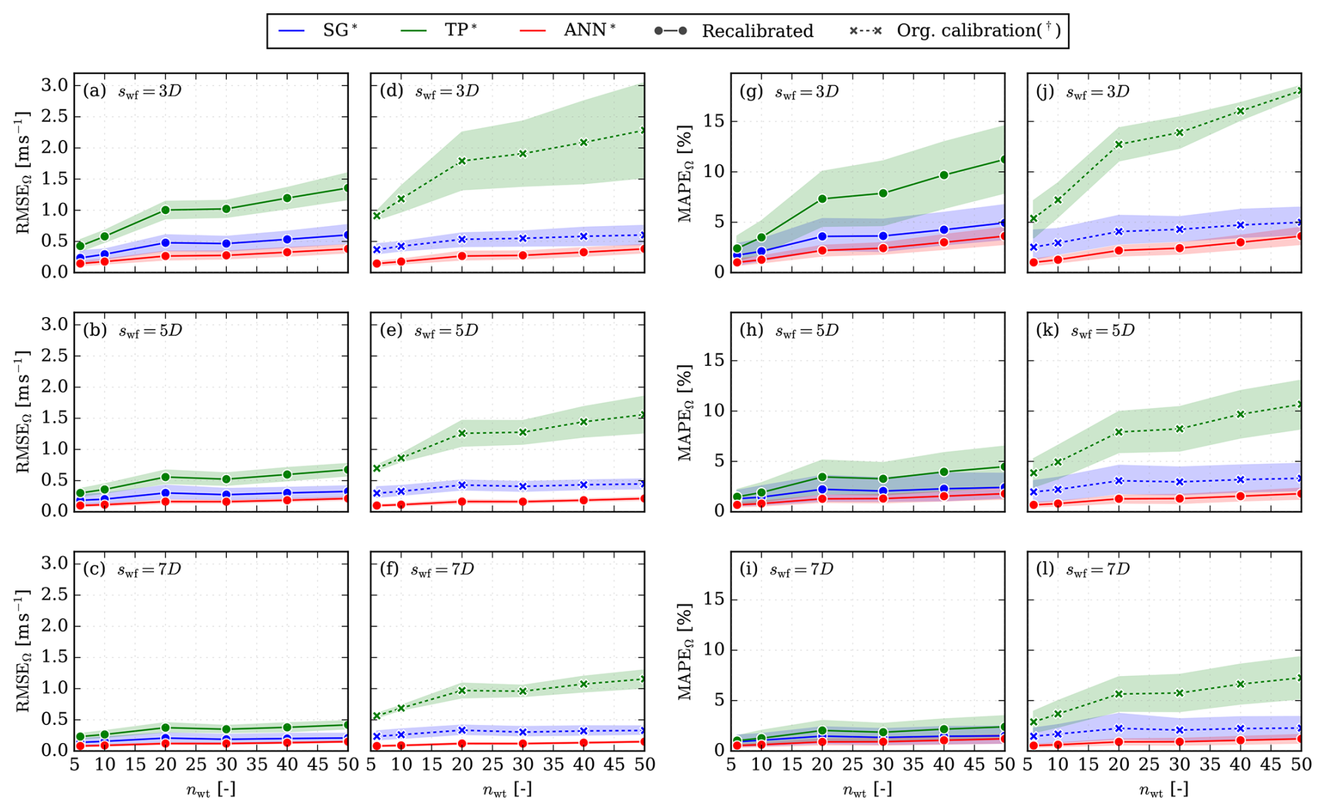
Figure A1 Flow study result metrics for an increasing number of wind turbines, with a blockage model. (a–c) RMSE with calibrated wake models, (d–f) RMSE with uncalibrated wake models, (g–i) MAPE with calibrated wake models, and (j–l) MAPE with uncalibrated wake models.

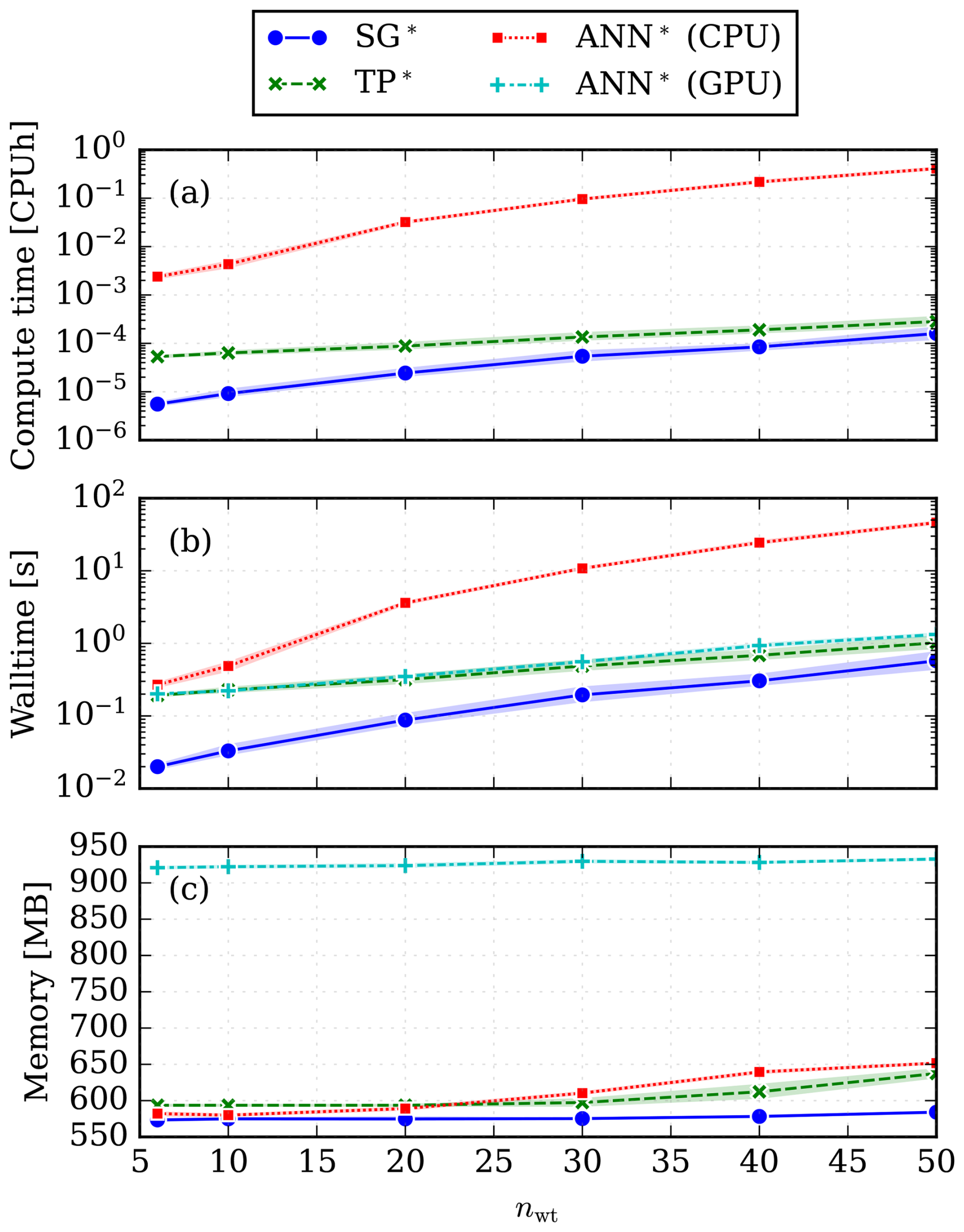
Figure A2 Average computational resource cost of a flow case for increasing wind farm sizes with inclusion of blockage. (a) Relative cost in CPU hours, (b) real-world cost in wall time (seconds), and (c) random access memory (RAM) consumption in MB.

Appendix B: Layouts obtained during WFLO

Figure B1 Initial and final layouts obtained through WFLO.

Appendix C: Flow study without blockage displayed on log scale

Figure C1 Flow study result metrics for an increasing number of wind turbines without a blockage model, displayed on a semi-logarithmic axis. Containing the same data as Fig. 6.

Appendix D: Multimodality experiment

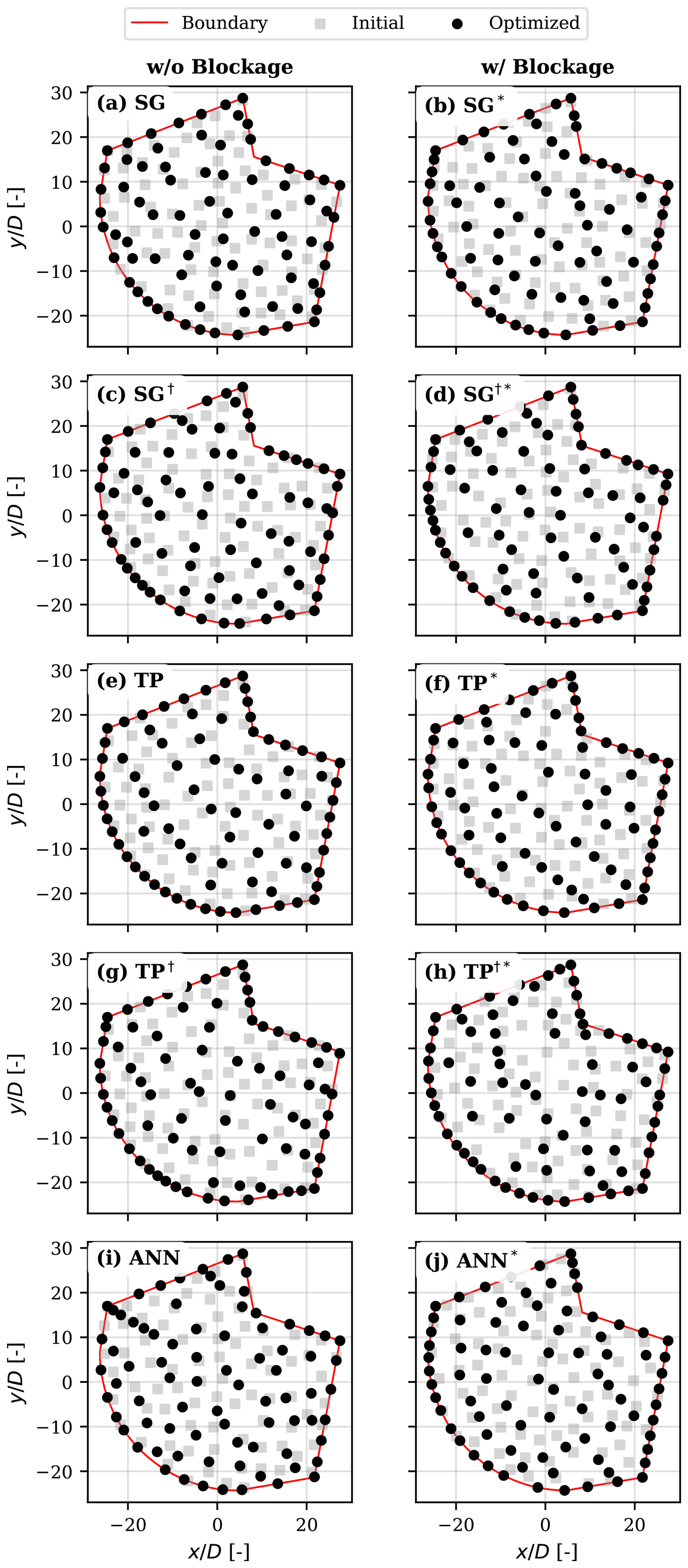
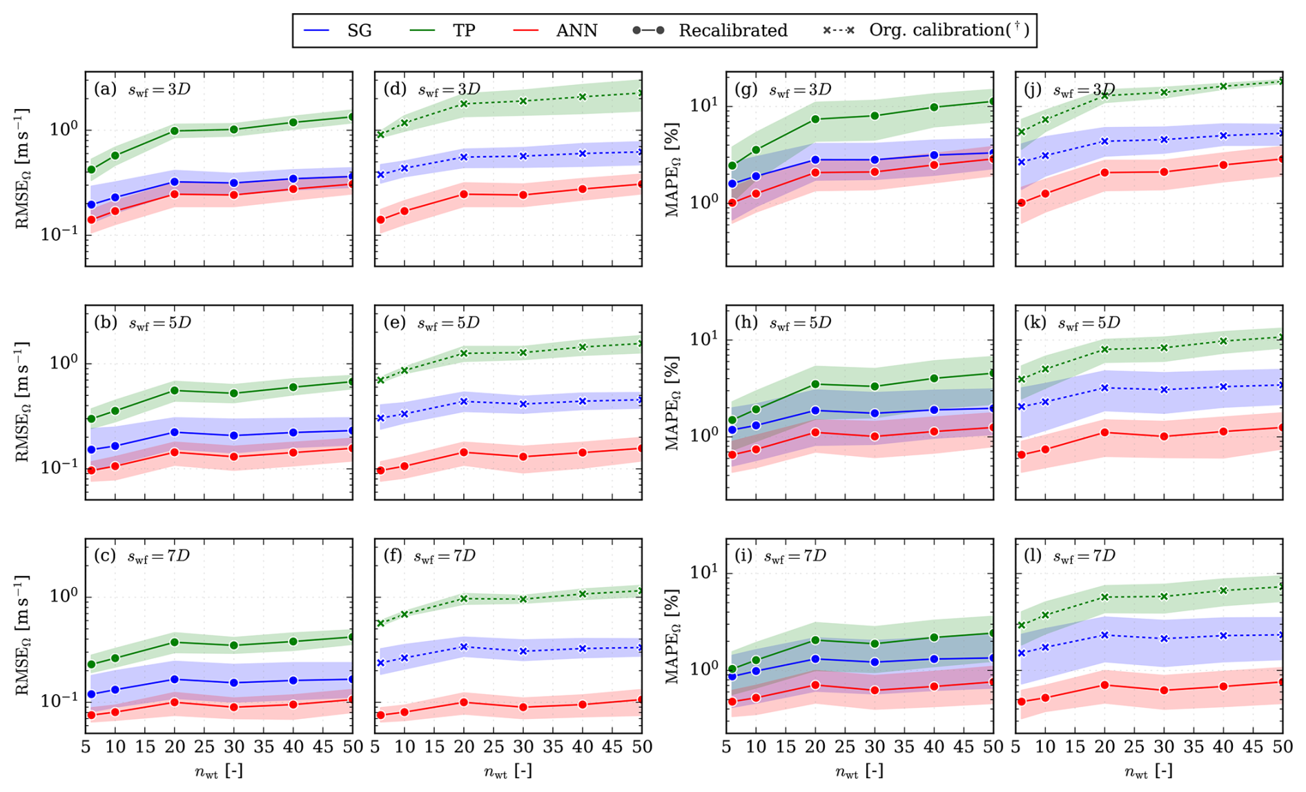
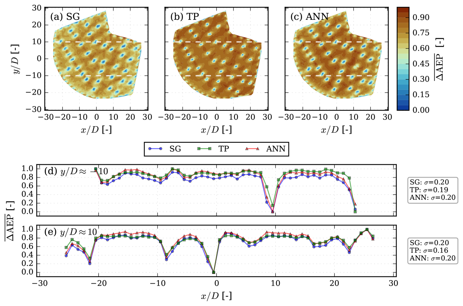
Figure D1 Objective function maps illustrating the normalized AEP improvement $\stackrel{\mathrm{‾}}{\mathrm{\Delta }\text{AEP}}$ for the calibrated low-fidelity models without blockage: (a) SG model, (b) TP model, and (c) ANN model with a cross-plane profile for all models (d) at $y/D\approx -\mathrm{10}$ and (e) at $y/D\approx \mathrm{10}$.

We investigated the hypothesis that the improved RANS AEP obtained using the TP model correlates with a lower degree of multimodality in the objective function. To do so, the SG, TP, and ANN models were employed to evaluate the improvement in AEP (ΔAEP) that could be achieved by adding a turbine to the best-performing layout obtained with the TP model by systematically assessing the addition of the turbine at different locations throughout the farm. In practice, a grid was constructed with a density of one grid point per D, and the AEP improvement (ΔAEP) was then evaluated for every possible location the additional turbine could be placed in the grid.

Because the ranges vary significantly, which obscures the perceived smoothness of the objective function map, ΔAEP is min–max normalized independently for each observation, placing all the results within a range of 0–1:

$$\begin{array}{}\text{(D1)}& {\displaystyle }{\displaystyle }\stackrel{\mathrm{‾}}{\mathrm{\Delta }\text{AEP}}(x,y)={\displaystyle \frac{\mathrm{\Delta }\text{AEP}(x,y)-{min}_{x,y}\left(\mathrm{\Delta }\text{AEP}\right)}{{max}_{x,y}\left(\mathrm{\Delta }\text{AEP}\right)}}.\end{array}$$

The resulting objective function maps, illustrating $\stackrel{\mathrm{‾}}{\mathrm{\Delta }\text{AEP}}$, are shown in Fig. D1. Additionally, two extra subplots are included, showing $\stackrel{\mathrm{‾}}{\mathrm{\Delta }\text{AEP}}$ at $y\approx \pm \mathrm{10}D$ for all three models in one plot at a time.

Figure D1a–c illustrate that there is slightly less variability in the range of $\stackrel{\mathrm{‾}}{\mathrm{\Delta }\text{AEP}}$ for the TP model compared to the other two models. In Fig. D1d and e, the cross-plane $\stackrel{\mathrm{‾}}{\mathrm{\Delta }\text{AEP}}$ is visualized. Here, the differences between the models are subtle: the TP model shows marginally smoother variations, with fewer extreme peaks and valleys, compared to SG and ANN, but the overall patterns remain broadly similar. As this can be difficult to see visually, SD (σ) values are displayed in Fig. D1d and e to quantify the variability in each cross-section. Lower values of σ indicate smoother objective function landscapes. Here, the TP model consistently shows the lowest σ, supporting the observation of reduced multimodality.