Experimental investigation of the effect of wake steering on the noise emission of a commercial wind turbine

Wake steering is a wind farm flow control (WFFC) strategy that involves intentionally misaligning the most upstream wind turbines to deviate their wakes away from the downstream wind turbines. This study investigates the acoustic implications of such a strategy. A novel acoustic setup is implemented, involving 24 ground-based sound level meters arranged on a circle around an industrial 2.2 MW wind turbine, positioned at tip-height distance. This configuration enables a fine angular resolution of 15°. Incoming wind conditions are monitored using both a nacelle-mounted and a ground-based lidar. A test protocol closely aligned with IEC 61400-11-1 is followed to characterize the turbine's noise emissions under various yaw misalignment settings, ranging from −20 to +20° across a broad spectrum of flow conditions. A dedicated data cleaning and analysis procedure is developed to derive ground-level turbine noise directivity patterns. In the absence of yaw misalignment, the directivity patterns exhibit a typical two-lobe structure. However, slight but statistically significant asymmetries are also observed: the downstroke side is on average 0.6 dB(A) louder than the upstroke side, and the downwind side is 0.4 dB(A) louder than the upwind side. These specificities are not captured by most of the analytical models used in the field. When yaw misalignment is applied, a modest increase of approximately 0.6 dB(A) is observed in the estimated overall sound power level. The results from this innovative experiment confirm the fact that operators must consider metrics other than just power production when implementing WFFC in their projects and that more advanced noise models are required for the development of a framework allowing multi-objective WFFC.

1 Introduction and context

Wind farm flow control (WFFC) is a concept in which turbines within a wind farm are controlled in a coordinated way to accomplish a common objective, such as increase in farm power production, reduction in turbine loading, or active power control (Boersma et al., 2017). Two strategies are generally considered to achieve these goals: the axial induction strategy, in which upstream turbines are down-regulated to leave more kinetic energy for downstream turbines, and the wake steering strategy, which consists of intentionally misaligning the upstream turbines to deflect the wake away from the downstream turbines. For both strategies, the performance of the most upstream turbines is reduced so that the performance of the downstream turbines is improved: the WFFC is successful when the downstream gain compensates for the upstream loss and the overall power production is increased. WFFC has been an intense subject of research over the past decade, with many full-scale experiments conducted all over the world on commercial wind farms (Meyers et al., 2022). The vast majority of these experiments were focused on the objective of improving the total energy production of a wind farm, while only a few of them tackled the issue of load reduction (Damiani et al., 2018; Dana et al., 2022) or active power control (Göçmen, 2016).

Among the two strategies, wake steering has shown greater potential for power improvements, with a track record of many full-scale field tests showing significant energy gains (see, e.g., Fleming et al., 2017, 2019, 2020, 2021; Simley et al., 2021; Doekemeijer et al., 2021; Howland et al., 2022). On the other hand, meaningful power gains seem more difficult to achieve through axial induction control, although a few full-scale experiments were able to highlight performance improvements for specific wind sectors (van der Hoek et al., 2019; Bossanyi and Ruisi, 2021). When averaging over the full wind rose to get the total annual energy gains, those gains are drastically reduced, and consequently this strategy might be more suitable for achieving load reduction and active power control (Boersma et al., 2017).

Another less widespread objective that can be achieved through WFFC is acoustic control of a wind farm (Nyborg et al., 2023). Wind turbines are controlled together to comply with local legislation and make sure the total noise emissions of the farm remain below a given threshold while trying to maximize the total energy production. This is usually accomplished using an axial induction strategy, during which specific noise-reduced operation (NRO) modes are activated according to a list of criteria (for instance time of day, period of year, incoming wind speed and direction sector). A practical example of an implemented acoustic curtailment plan is presented in Fig. 1. Note that it is usually defined using numerical simulations and simple noise source models assuming omnidirectional noise sources. A variation of ±0.5 dB(A) in the source power definition can be qualified as “small” from an acceptance point of view since it is lower than 1 dB, the level variation threshold of human hearing. However, in critical situations, such variation can lead to significant changes in the curtailment plan associated with variations in annual energy production (AEP) of the order of 1 % since the chosen curtailment plan must strictly comply with local noise regulations.

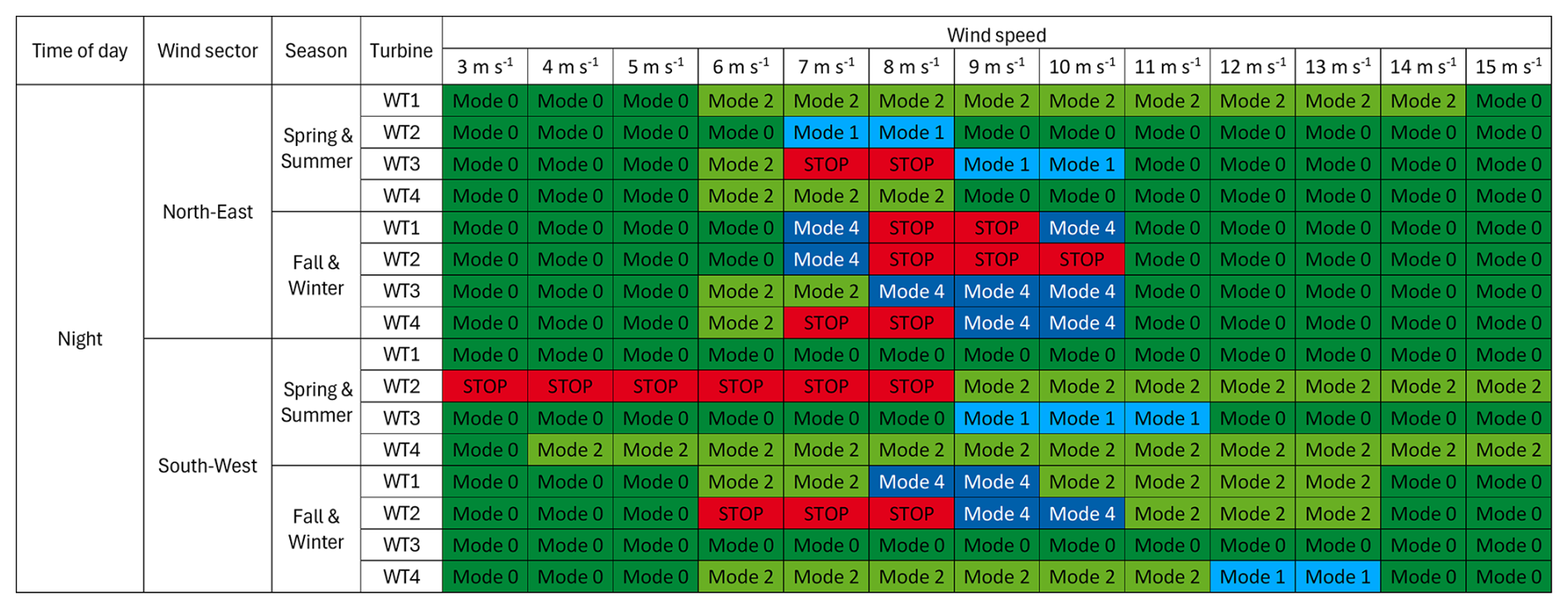
Figure 1 Typical acoustic curtailment applied in a wind farm. The wind farm control is applied as a look-up table giving the NRO mode to be followed by each turbine as a function of several environmental criteria. The turbines are supposed to be operated in full power mode outside the conditions provided in this look-up table (e.g., during daytime).

An expert elicitation about WFFC conducted a few years ago ranked the noise reduction objective in only the second to last position (van Wingerden et al., 2020). However, in some countries where regulations and constraints are very restrictive, the topic of farm noise emissions has become increasingly important. As an example, the large majority of newly developed wind projects in France are now concerned with an acoustic curtailment, leading to a 2.8 % average reduction in AEP (Willis, 2023).

The TWAIN research project (TWAIN, 2023) aims at providing a framework for multi-objective WFFC: an increase in power production, a reduction in turbine loading, and complying with grid requirements or environmental regulations (acoustics, wildlife, and social consciousness). Therefore, understanding the impact of WFFC actions not only on turbine power and loads but also on other aspects, such as farm noise emissions, is critical for designing optimal strategies to be applied by the wind farm owner or operator. In that scope, acoustic models must be improved and validated to bridge the gap with the current state of the art.

Noise impact studies dedicated to permitting industrial wind farm projects most often involve omnidirectional point noise sources located at the nacelle center of wind turbines. However, several scientific studies challenge this omnidirectionality assumption. Acoustic measurements on full-scale wind turbines consistently show a “noise dip” of a few decibels in the rotor plane (Oerlemans and Schepers, 2009; Buck et al., 2016; Okada et al., 2016), which is generally reproduced by more advanced analytical models. In contrast, complex multi-lobe structures and upwind/downwind and upstroke/downstroke asymmetries are observed but not fully captured by those models.

Similarly, while axial induction control has been used for years to implement the acoustic curtailment plan, the effect of wake steering on noise emissions remains an open question. Only two full-scale experiments related to this topic were found in the literature, with one pointing toward a reduction in the noise emission due to the application of yaw misalignment (Hamilton et al., 2021) and the other showing no hearable impact (Bonsma et al., 2019). Since wake steering has already demonstrated positive energy gains and has begun to be deployed on many wind farms (Harrison et al., 2025), there is a need to quantify its impacts on acoustics more accurately.

This paper introduces a novel field campaign designed specifically to study the effect of turbine yaw misalignment on sound magnitude and directivity. A commercial wind turbine has been fully surrounded by 24 sound level meters (SLMs) in order to measure the directivity pattern of its noise emissions with a high resolution and track how it is changed when yaw misalignment is applied. In the following, the term “directivity” refers to the ground trace of the horizontal noise directivity, as measured by a circle of SLMs around the turbine.

The field campaign, described in Sect. 2, was prepared following the recommendations of the IEC 61400-11-1 standard as close as possible (IEC, 2012), and therefore terms and notations adopted in this article are mostly inspired from this reference. However, due to the extensivity of the setup, a few adjustments to the standard procedure had to be applied. Those are detailed in Sect. 3 along with the methodology applied to process the large dataset recorded during the campaign. Section 4 provides the analysis of noise directivity patterns and the effect of yaw misalignment. The goal of this experiment is to provide a high-quality dataset that can be used within the TWAIN project to improve acoustics models; Sect. 5 thus concludes this paper and offers perspectives about future developments realized in the scope of the project.

2 Description of the field campaign

The field campaign was conducted from 25 to 28 March 2024 on a commercial wind turbine (diameter D=110 m, nominal power P=2.2 MW, and hub height HH = 80 m) in a farm operated by ENGIE Green and located in the northern region of France. This section gives a summary of the experimental setup, the procedure followed, and the wind conditions recorded during the test.

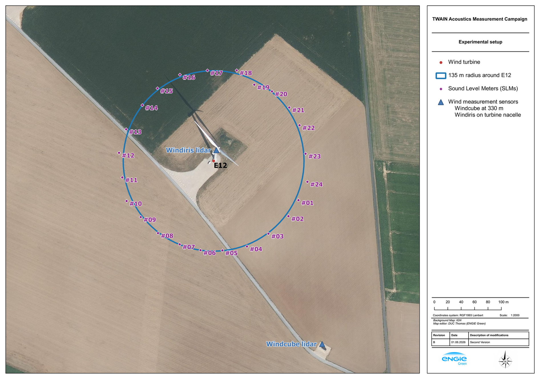
Figure 2 Experimental setup of the TWAIN acoustic measurement campaign. External wind sensors include a ground-based Windcube lidar located at 330 m from the turbine and a nacelle-mounted Windiris lidar. The 24 sound level meters were placed approximately one turbine total height (135 m) from the tower base.

2.1 Experimental setup

Figure 2 recaps the experimental setup that was implemented during the campaign. The 24 sound level meters (SLMs) surrounding the turbine were located every 15° at a distance of approximately one turbine tip height (135 m) from the turbine. Distance to the tower base was measured using a laser pointer and verified by comparing the GPS coordinates of the turbines and each SLM. The obtained values ranged from 132.5 to 139.4 m, which is consistent with the ±20 % and ±30 m tolerance criteria of the IEC standard (IEC, 2012). The angular difference between two successive SLMs was evaluated using their GPS coordinates and varied from 11.6 to 18.2°. The distance from the ground-based Windcube lidar to the turbine was also estimated based on its GPS coordinates and found to be roughly 330 m.

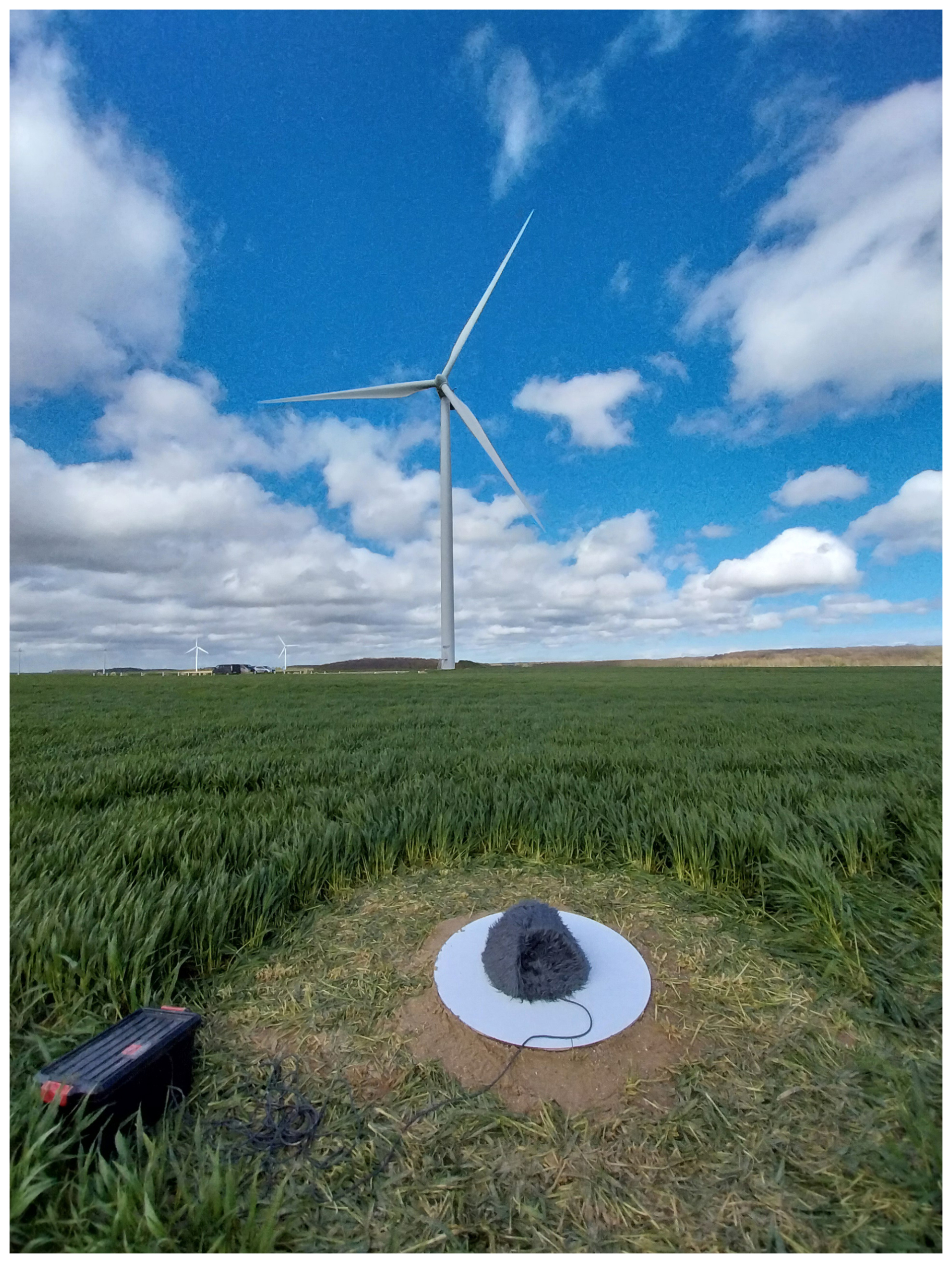
The site is very simple and flat, and the calculated terrain inclination angle ϕ (defined in the standard with the line joining the SLM and the turbine hub) for all positions varied between 29 and 31.5°, well within the 25–40° preconized range. The surrounding terrain mostly consists of wheat crops. In late March, at the time of the experiment, those crops reached a height of about 30 cm. In order to prevent any disturbance caused by the crops' wind-induced noise, they were cut within a diameter of roughly 3 m around each SLM position. Figure 3 shows one SLM together with a controlled turbine in the background.

Figure 3 Picture of one SLM with E12 wind turbine in the background. The wheat crops around the SLM were cut to prevent noise disturbance. Following the recommendations of the IEC standard (IEC, 2012), all SLMs are installed on a woodboard of 1 m diameter and covered by two windscreens.

SCADA data for the misaligned turbine were collected during the test at 1 s resolution for the most important variables: active power, wind speed, vane angle, nacelle position, rotor and generator speed, and pitch angle. Almost all acoustics sensors were removed each night and reinstalled every morning at the same location. They were checked for time synchronization and calibration before new measurements were launched. Both the overall sound pressure levels and the $\mathrm{1}/\mathrm{3}$-octave band spectra were recorded with a sampling period of 1 s. Lidar measurements were acquired at an identical temporal resolution.

2.2 Test procedure

In order to study the effect of yaw misalignment on wind turbine noise in similar atmospheric conditions, a specific measurement routine was designed for the campaign. The yaw set point parameter β is defined as the angle between the nacelle axis and the incoming main flow direction. The turbine was sequentially yawed from $\mathit{\beta }=-\mathrm{20}$ to $\mathit{\beta }=+\mathrm{20}$° in steps of 10°, staying in each position for 40 min. Between two successive positions, background noise and turbine noise measurements were also conducted with β=0°, each of them lasting 10 min. Finally, a period of 3 min was considered for each transition to give the turbine some time to move or restart and let the flow reach its equilibrium for the new position. The full routine, planned to last almost 4.5 h, can be found in Table 1.

Table 1 Description of the measurement routine followed during the test. Each phase is planned to last 40 min. The background noise and turbine noise measurements at β=0° are spread out into four steps of 10 min each to be recorded closer to the misaligned conditions.

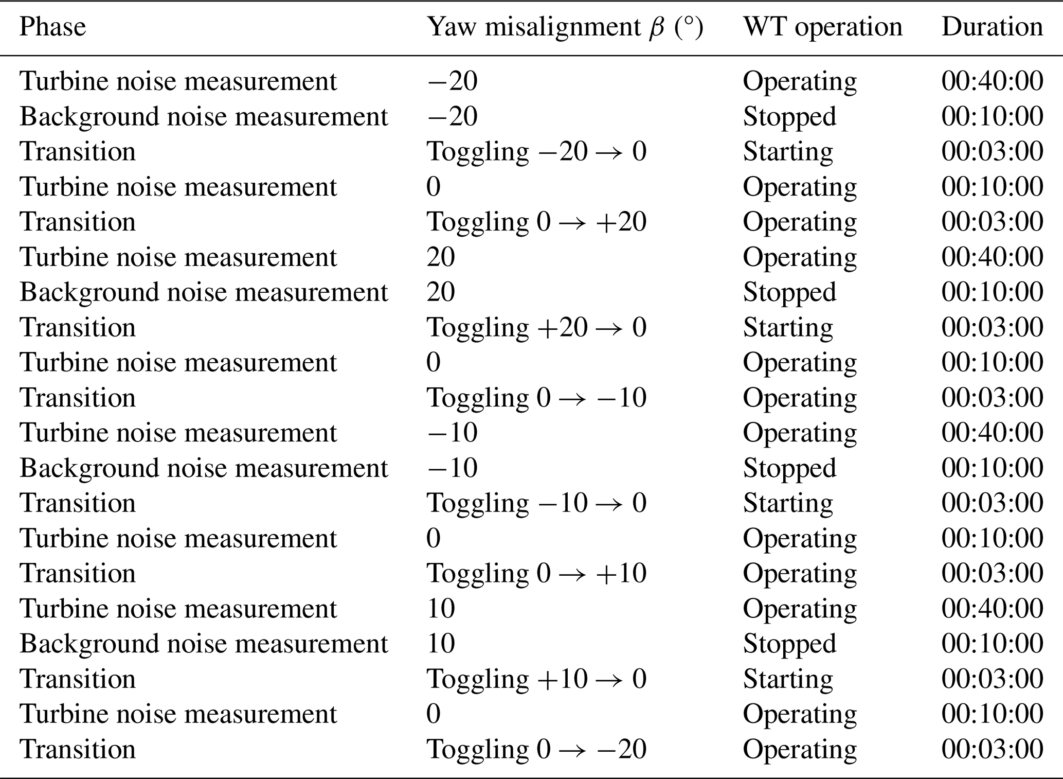
In practice, this routine could not be programmed in the control software, and the turbine was manually switched between each state by an operator. The periods in each position were thus approximately followed but were maintained at least as long as indicated above. Overall, the fulfillment of one full round of measurement lasted slightly longer than originally planned. During the data post-processing, the SCADA 1 s time series of active power and nacelle position were visually inspected to precisely mark the exact timestamps of switching from one phase to another. In operation phases, the target turbine was settled to the full power mode, i.e., without any NRO mode implemented.

The two nearest turbines in the farm (WT10 and WT11, located 345 and 770 m northwest of WT12, respectively) were shut down at the beginning of each round of measurement and remained stopped for the full duration of the test to avoid disturbing the test and recording data and ensure a satisfactory signal to noise ratio. The closest neighboring turbine still in operation was located more than 1 km away. A person was also constantly present on site to keep a track record of noisy events (such as a plane or car passing by) so that they could be properly considered and filtered afterwards.

2.3 Wind conditions recorded during the test

The experiment consisted of six rounds of measurements that were conducted over the 4 d: one on 25 March 2024 and on 26 March 2024 and two on 27 March 2024 and 28 March 2024. Rounds 2, 4, and 6 could not be conducted completely due to the appearance of rain in the afternoon of the 26th and 27th and strong and highly turbulent winds risking the endangerment of the turbine during yaw misalignment conditions in the late afternoon of the 28th. Considering that these above-rated conditions are of less importance to WFFC applications, these data would not have added much additional value. In total, a little more than 21 h of measurements was recorded over the 4 d (4.58 h on day 1, 2.35 h on day 2, 6.13 h on day 3, and 8.07 h on day 4).

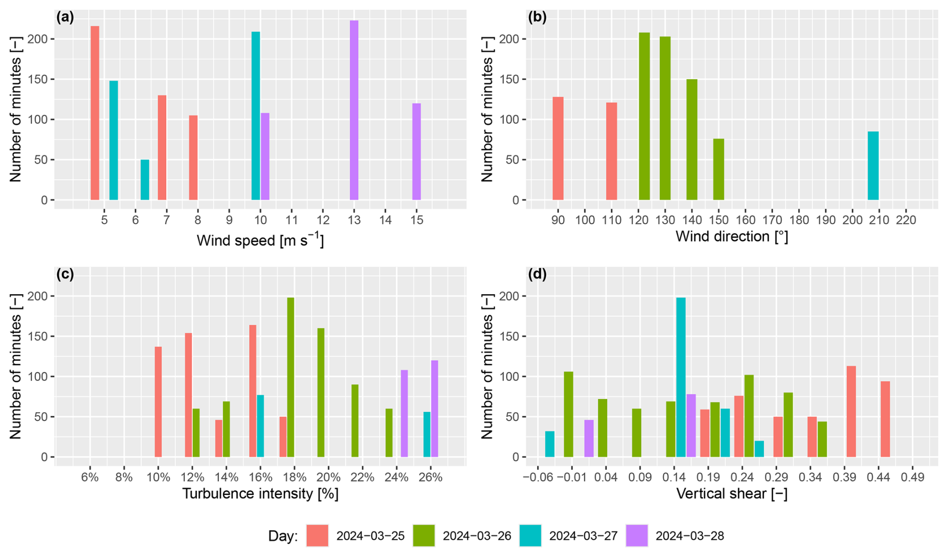
Figure 4 Wind conditions recorded during the field campaign. Histogram of occurrences of wind speed (a), wind direction (b), turbulence intensity (c), and wind shear (d) for each day of measurement.

The wind conditions observed during the campaign are represented in Fig. 4. Very different conditions were experienced each day: from low to medium wind speeds during the first 2 d to higher wind speeds on the last 2 d. The IEC standard requires a minimum number of 10 samples in each bin. As can be seen in Fig. 5 in the representation of the raw capture matrix derived from the SCADA data recorded during the six rounds of the test, these criteria are fulfilled for a large number of wind speed bins and all yaw positions thanks to those very favorable wind conditions. Consequently, the minimum wind speed range recommended by the standard, 8 to 13.5 m s⁻¹ (corresponding to 0.8 to 1.3 times the wind speed at 85 % of the turbine rated power), was extended to 6–13.5 m s⁻¹ when analyzing the results.

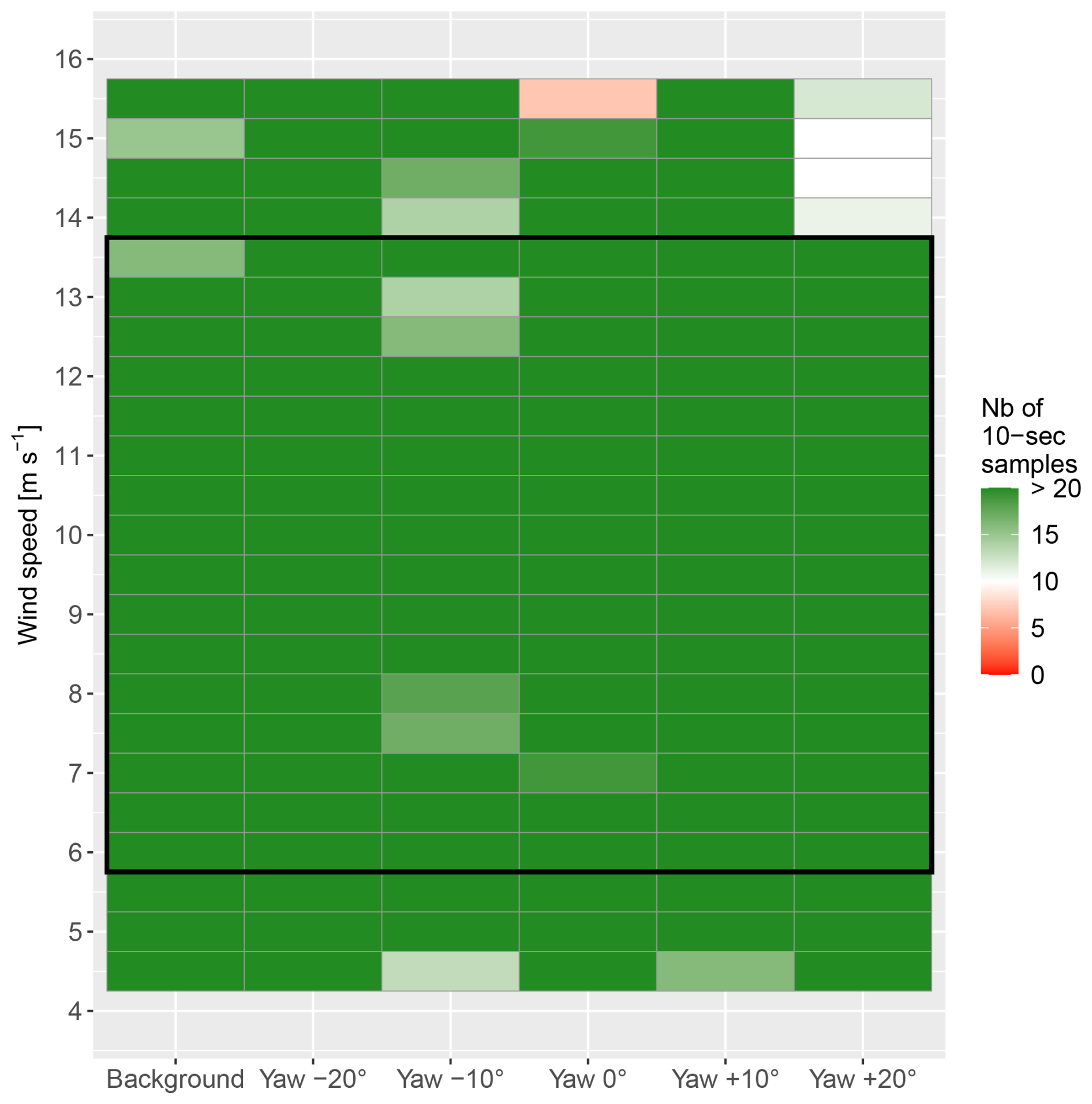
Figure 5 Raw capture matrix for the TWAIN acoustic campaign. The number of 10 s samples is shown for each wind speed bin and each yaw misalignment case. The black rectangle represents the wind speed range of interest between 6 and 13.5 m s⁻¹.

The wind direction varied from the east on the first day to the southwest on the last day, meaning that the turbine was never affected by any wakes during the measurement. Turbulence and shear conditions were estimated using the ground-based Windcube lidar: the lidar measurement at hub height is considered for the turbulence, while the wind shear is estimated by fitting a power law to 14 planes of measurement ranging from 40 to 140 m (i.e., the span of the turbine rotor). Both were also very variable depending on the day, with high shear and low turbulence observed at the beginning of the week and, in contrast, a highly turbulent and low-sheared flow noticed at the end of the test.

2.4 Data availability

A significant challenge for a field campaign utilizing as many sensors as this one is to maintain the availability of all of them during the periods of measurement. Figures 6 and 7 represent the availability of related wind and acoustic sensors, respectively, indicating that this challenge was practically met.

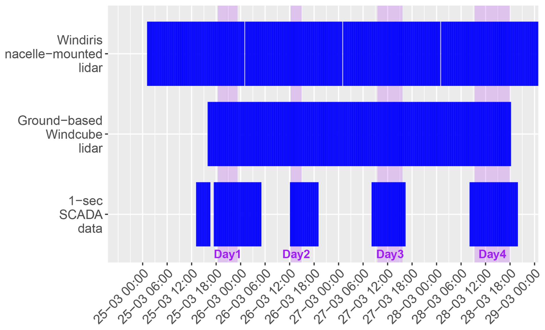
Figure 6 Availability of related wind sensors during the TWAIN acoustic campaign. The purple-shaded vertical bands indicate active measurement for each day.

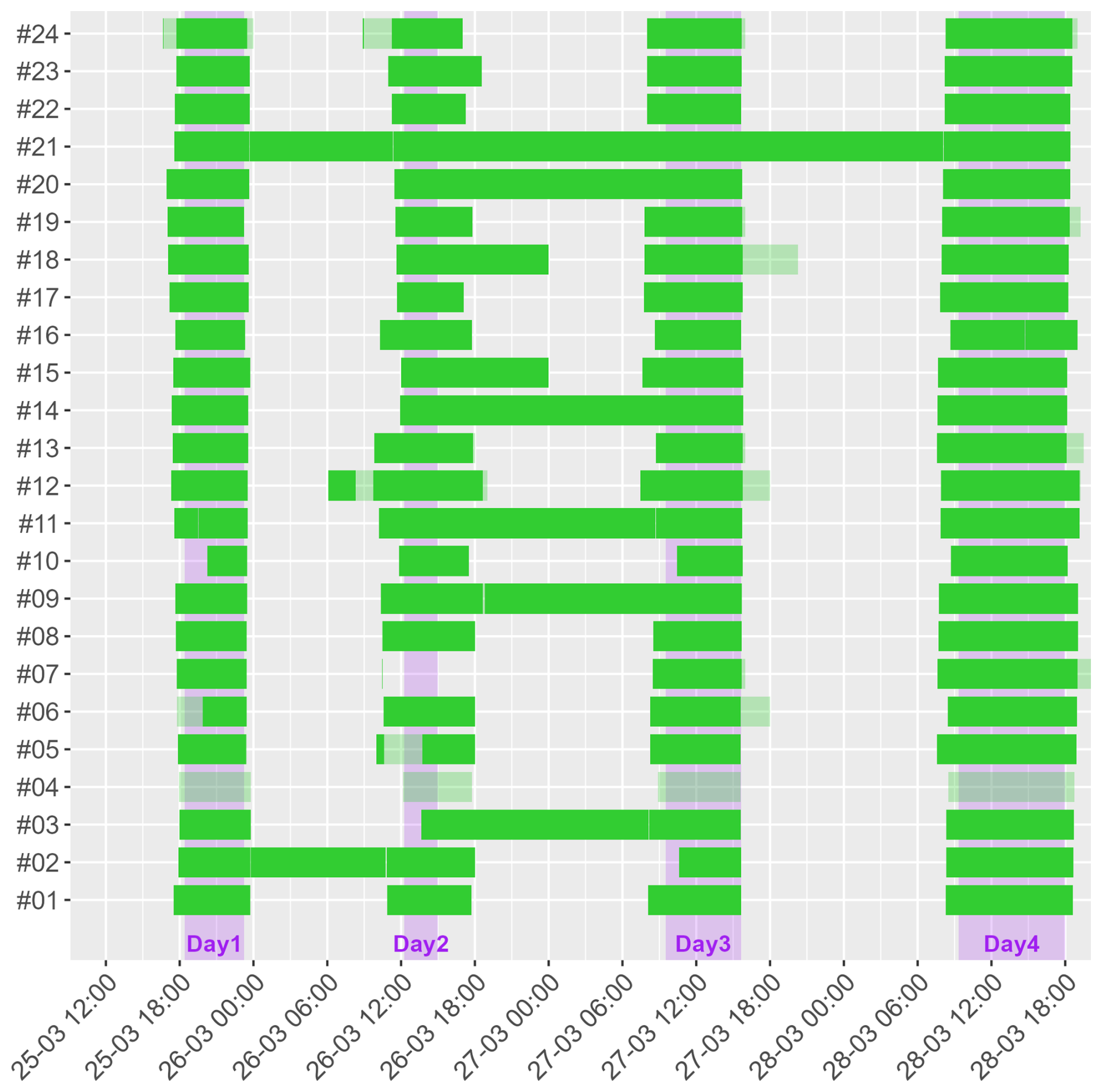
Figure 7 Availability of overall sound pressure level data for all SLMs during the TWAIN acoustic campaign. A transparent band (e.g., for SLM no. 4) corresponds to a reduced availability. The purple-shaded vertical bands indicate active measurement for each day.

Most of the SLMs were also fully available during the test. Unfortunately, a few sensor defaults were observed when preprocessing the data. SLM no. 4 shows only a 10 % availability because it was only possible to record data every 10 s instead of 1 s due to a logger issue. SLM no. 7 reports reduced availability since it was not installed during the second day of measurement. The IEC standard also requires an analysis of $\mathrm{1}/\mathrm{3}$-octave bands between 20 Hz and 10 kHz. A full dataset was obtained for 18 SLMs, but $\mathrm{1}/\mathrm{3}$-octave information was missing for SLM nos. 9 and 18 and incomplete for nos. 4, 10, 16, 21, and 22.

Despite these small inconveniences, the quantity of data collected during the 4 d and six rounds of measurement can be considered satisfactory and ready to be processed for the derivation of the apparent sound power level, as is described in the next section.

3 Data processing

The IEC 61400-11-1 standard defines a procedure for the processing of data recorded during an acoustic noise measurement campaign: aggregation of data into 10 s chunks, time synchronization between acoustics and wind-related sensors, estimation of ambient wind speed, normalization of $\mathrm{1}/\mathrm{3}$-octave band spectra and correction for secondary wind screen, sorting into bins, computation of average and standard deviation acoustic values on bin centers, and computation of apparent sound power spectra through the difference between the total noise and background noise values.

However, this procedure corresponds to the case of a single SLM placed directly downstream of a turbine aligned with the wind direction. Due to the novelty of this campaign in utilizing a large number of SLMs and the application of yaw misalignment to the turbine, some adjustments to the standard procedure were necessary.

3.1 Acoustic data cleaning

The process described above must be performed on a cleaned dataset. Despite the effort made every day during the campaign to calibrate and check the time synchronization of each SLM before launching a new round of measurement, a few issues were noticed when the raw acoustics data were analyzed. Considering the large quantity of data to handle (more than 507 h when accounting for the 24 SLMs), specific post-processing techniques were designed to automatically filter and correct the dataset.

3.1.1 Time synchronization

The most significant issue observed during data inspection was related to the time synchronization of the acoustic signals. Indeed, during the campaign, each SLM was recording data using its own internal clock. Although each clock was verified at the beginning of a new measurement, it proved insufficient to ensure a proper synchronization of the signals, and time shifts were found when inspecting the recorded time series. These time shifts were seen to be dependent on both the day and the sensor. Figure 8 shows an example in which two SLMs clearly seem out of sync with respect to the rest of the fleet.

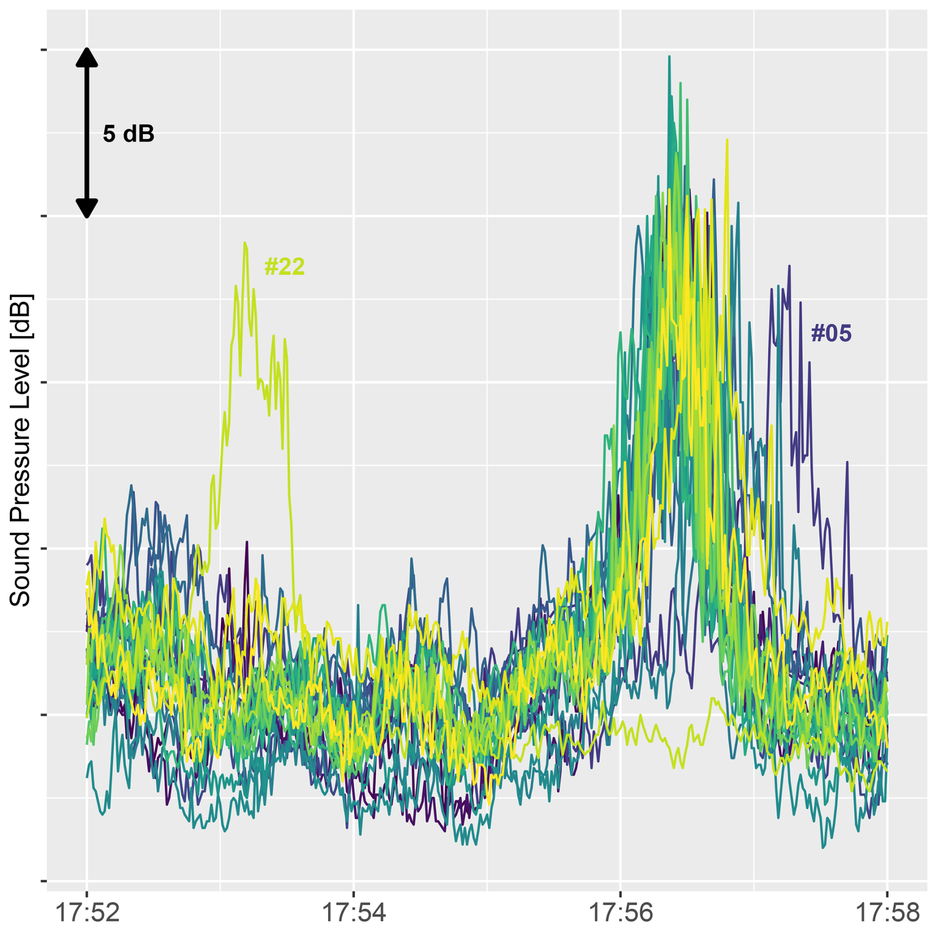
Figure 8 Illustration of a time sync issue during day 4. The passing of a plane increases the sound pressure level of all SLMs between 17:56 and 17:57 CET. This is captured by all of them at more or less the same time, except for SLM no. 22, which appears to be ahead, and SLM no. 5, which is delayed.

In order to identify and correct those time shifts en masse, the following methodology was applied for each day of measurement.

1. For each pair of SLMs, a cross-correlation curve is obtained by sliding the time signals at steps of 1 s over ±600 s.

2. The time delay that corresponds to the maximum of this cross-correlation curve is inserted into a matrix of time shifts that stores the most likely delay for each couple of SLMs for a given day of measurement.

3. A unique time shift per SLM is deduced by solving a linear optimization problem.

4. Finally, the acoustic signals are resynchronized with the turbine SCADA clock by using another cross-correlation analysis with the electrical power signal (and taking advantage of the background noise measurement periods when the power suddenly drops to 0 kW with a an immediate reduction in its noise emissions).

The first three steps of the methodology are performed to ensure better robustness of the clock drift correction thanks to the comparison of multiple SLM pairs. The last one is allowed by the fact that the subject of the study is focused on energetic aspects rather than on acoustic propagation time. The distance between the main acoustic sources (the blade outer part for aerodynamic noise and the nacelle for mechanical noise) is at most around 300 m, so the dispersion of acoustic propagation times remains of the order of a second. Given that the data are then aggregated into 10 s chunks for the rest of the IEC analysis, the uncertainty related to this correction is small. A sensitivity analysis was run on the results by shifting all the acoustics signals by ±1 s and showed that this effect only had a negligible impact.

A summary of the calculated time shift for all SLMs and all days of measurement is shown in Fig. 9. It can be seen that the vast majority of the introduced corrections are within ±15 s. Nonetheless, significant delays were applied for some SLMs: −547 s was found for SLM no. 15 on days 1 and 2, and +192 s was obtained for SLM no. 22 on day 4 in accordance with the visual observations in Fig. 8.

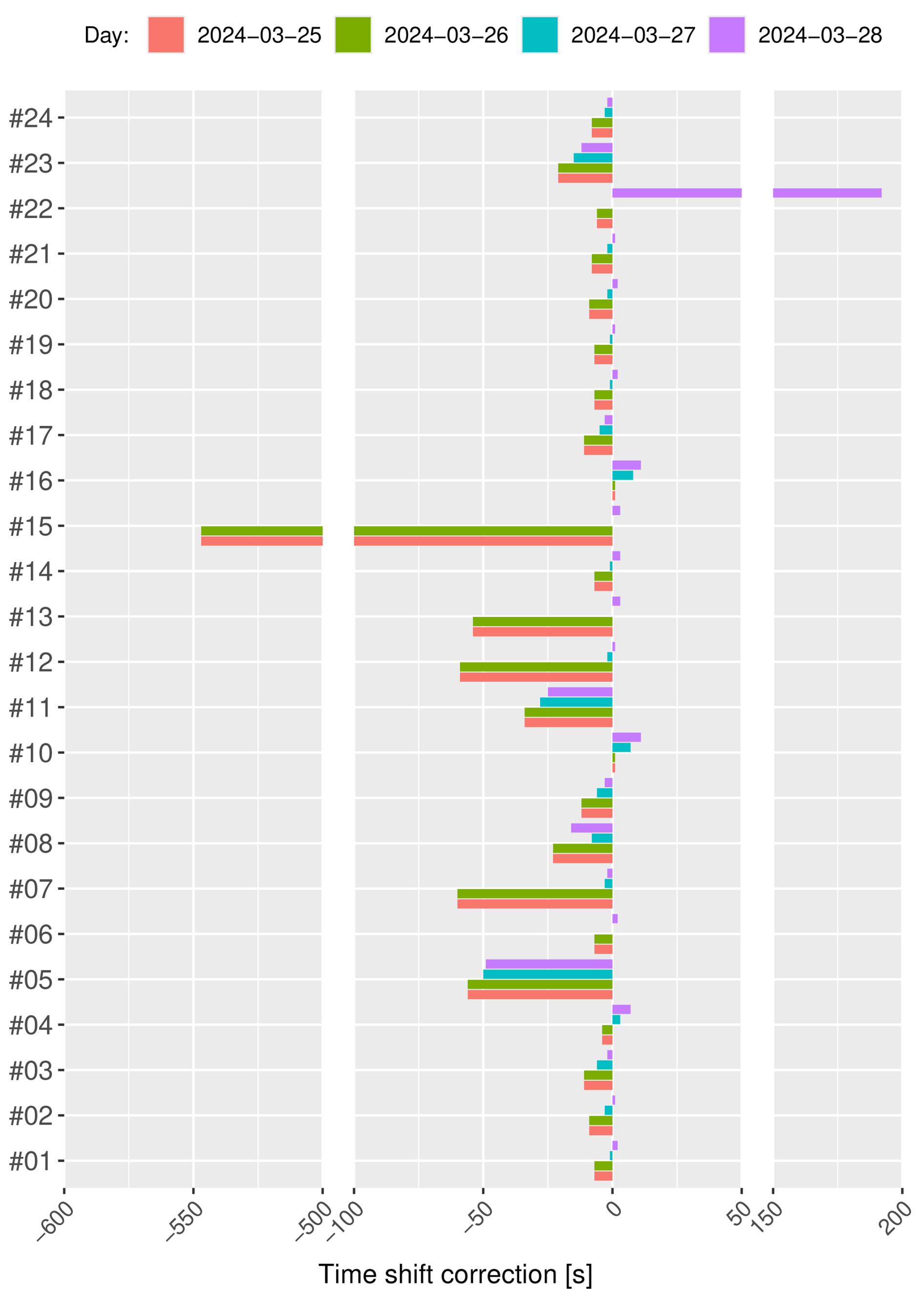
Figure 9 Time shift corrections applied for each SLM and each day of measurement. 0 s represents a perfect synchronization with the SCADA, a positive (negative) value is found when the SLM data are ahead (delayed) with respect to the SCADA.

3.1.2 Noisy events and outlier removal

The requirements of the IEC 61400-11-1 standard indicate that periods with intermittent background noise should be omitted from the analysis. As already explained in Sect. 2 above, an operator was always present on site during the period of measurement to take note of the time when noisy events were heard (e.g., aircraft, cars, agricultural machineries). The 1 s acoustic signals of each SLM were visually inspected to identify the starting and ending times of each event with some security margin (see, e.g., Fig. 8 for an example of a plane passing), and the corresponding periods were filtered accordingly.

However, despite this first filter based on the observer's notes, it was observed that a few remaining abnormal data could not be related to any recorded noisy events. Those outliers are characterized by sudden peaks in the acoustic signals. All impulsive events (the external ones and the ones originating from the turbine) are unwanted, as this study primarily focuses on turbine pseudo-stationary noise sources. To automatically detect and remove those points, a running median filter (Tukey, 1977) has been set up. Without visual field information, the parameters of the filter have been tuned to automatically reproduce the a posteriori detection performed by a human expert on a reduced dataset. The expert was asked to identify obvious outliers in the OASPL time series recorded by SLM no. 01. The main parameters of the automatic detection tool are the length of the rolling median window, the detection threshold, and the length of the removal window. They have been manually chosen to provide a satisfactory proportion of correctly detected outliers while avoiding false positives. The selected parameter values achieve a recall of 64 % (i.e., 64 % of expert-identified events are correctly detected) and a precision of 100 % with respect to the expert reference, meaning that all automatically detected events correspond to events identified by the expert. In the end, the filter, applied on the full dataset, consists of the following steps: a ±50 s running median of the acoustic signal is calculated. Every time the original signal goes 10 dB above the running median, an outlier is marked, and data within ±20 s around this point are filtered. The full process is illustrated in Fig. 10. A spike in SPL around 21:42 is not removed as an outlier since the level does not reach the +10 dB threshold over the running median. This event is actually believed to originate from the turbine itself, as it systematically appears a few seconds before each turbine stop, occurring here between 21:40 and 21:55. It may be linked to noisy events in the turbine shutdown procedure. Since this phenomenon occurs systematically during an on–off transition, it is naturally filtered out as a transient period since the turbine is transitioning to a new operational state.

A total of 2150 outliers were identified thanks to this method for the 24 SLMs over the 4 d of the campaign, with disparate behaviors depending on the sensors. Since the subsequent processing, based on the IEC 61400-11-1 standard, relies heavily on median computations, it is inherently robust to residual outliers and reasonably independent of the filter parameter values. Repeating the whole data processing step with a more restrictive filter, using a level threshold of 5 dB above a ±25 s rolling median, raised the total outlier count to 4616 and showed a minimal mean absolute deviation in output sound power levels (below 0.04 dB).

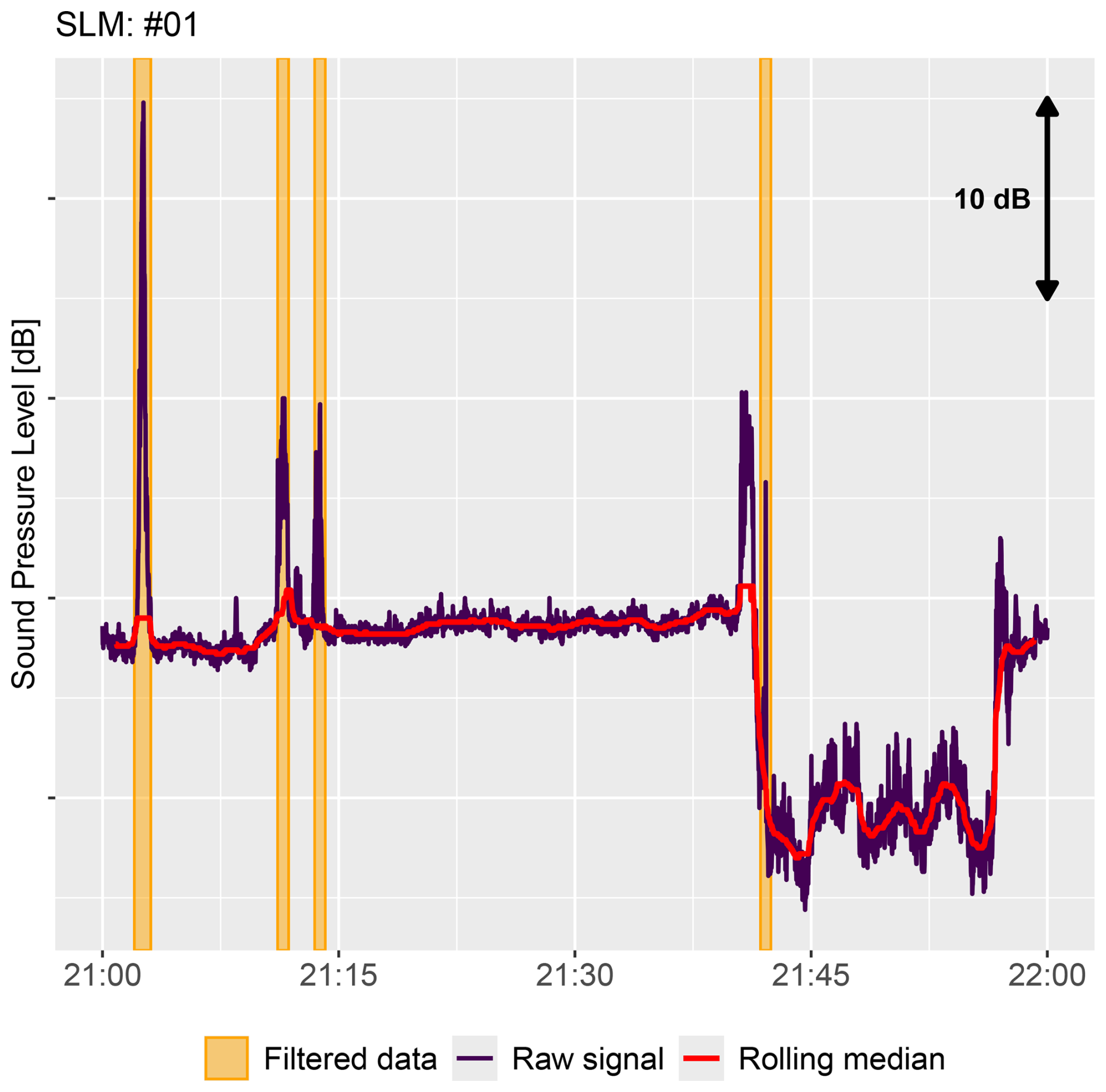
Figure 10 An example of automatic outlier detection for SLM no. 1. The rolling median is calculated from the raw signal, and periods of ±20 s above the +10 dB threshold are detected and removed. The turbine is shut down between 21:44 and 21:57 CET.

3.1.3 Final adjustments and aggregation

In addition to the above-mentioned cleaning applied to all SLMs, a few individual adjustments were also implemented to correct specific issues.

• SLM no. 6 showed a very low noise level for a few hours during day 1 despite a normal calibration procedure. This behavior was not repeated the following days of the campaign and could not be explained by the SLM manufacturer other than as being caused by a bad connection. These suspicious data have been discarded.

• SLM no. 21 only recorded $\mathrm{1}/\mathrm{1}$-octave data instead of $\mathrm{1}/\mathrm{3}$-octave data. The $\mathrm{1}/\mathrm{3}$-octave band was obtained through a linear interpolation of the $\mathrm{1}/\mathrm{1}$-octave band data, with the additional constraint of making sure that the sum of energy of the three calculated consecutive $\mathrm{1}/\mathrm{3}$-octave bands was consistent with the measured level for the corresponding $\mathrm{1}/\mathrm{1}$-octave band.

After those final corrections, the data preprocessing steps defined in the IEC procedure were followed. All signals were first aggregated into 10 s chunks, then the $\mathrm{1}/\mathrm{3}$-octave data were normalized to the measured overall sound pressure level, and the correction for the secondary wind screen was applied.

3.2 Identification of reference wind conditions

The data reduction procedure described in the IEC standard stipulates that the data must be binned by wind speed. The reference wind speed to be used for the binning is deduced from the active power signal by inverting the turbine power curve. The (adjusted) nacelle anemometer and external wind sensors are used as an alternative source of data when the power curve cannot be used (i.e., when the nominal power is reached or when the turbine is stopped for background measurement).

However, this methodology is only valid for a turbine that is aligned with the wind. Indeed, the performance of a steering turbine is reduced and no longer follows the expected power curve. Measurements from nacelle anemometers are also known to be unreliable when yaw misalignment is applied on a turbine (Kanev, 2020; Astolfi et al., 2023). It was thus necessary to adapt the IEC methodology to account for the specificity of this test.

For this field campaign, the reference wind speed signal was calculated according to the following, in order of priority.

1. When the turbine was operating with no yaw misalignment and the wind speed was within the allowed range for interpolation prescribed by the standard, the active power signal and the power curve were used. These conditions represent approximately 9 % of the total dataset. The power curve considered for the interpolation was calculated thanks to the nacelle lidar data over 4 months of measurements from 7 February to 2 June 2024 and according to the procedure of the IEC 61400-12-1 standard (IEC, 2017).

2. When the turbine was operating with no yaw misalignment but the wind speed was outside the allowed interpolation range, the nacelle anemometer, adjusted with a factor κ_nac=0.984, was chosen. Only 6 % of the data fall into this category.

3. During background noise measurement or when yaw misalignment was applied to the turbine (i.e., the remaining 85 % of the dataset), the measurement of the nacelle lidar at 300 m upstream (2.7 rotor diameters), adjusted with a factor κ_z=0.931, was selected.

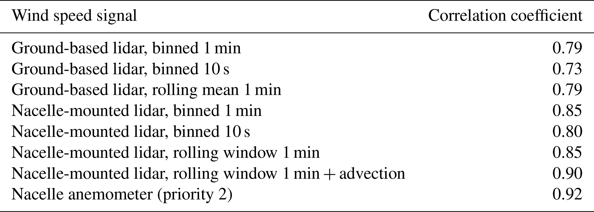
This sensor was favored over the ground-based lidar because its wind speed measurements were better correlated to the wind speed derived from the active power signal in step 1 above, as is shown in Table 2. Given that a transient period of 3 min was considered between each yaw category (see the toggle measurement routine in Table 1), there were no direct transitions between the nacelle lidar measurement and the SCADA signals, thus avoiding the risk of introducing artifacts between the different sources.

The high-frequency measurement of such a lidar is only conducted along line of sights (LOSs) of the sensor. Data from the 4 LOSs must be averaged over a certain time period and combined to derive the hub height wind speed estimation (Mazoyer and Boquet, 2016). Unfortunately, it proved that the 10 s resolution was too short to properly achieve this reconstruction: the resulting wind speed signal was too noisy and did not correlate well with the SCADA data. While complex algorithms exist to assess the incoming wind field from high-frequency lidar measurements (Raach et al., 2014; Borraccino et al., 2017; Guillemin et al., 2018), another solution was set up instead, for the sake of simplicity. For each day, a constant advection time was calculated using the mean wind speed observed during the recording period and the distance between the upstream lidar measurement range and the turbine. This advection time was used to temporally shift the lidar data and synchronize them with the rotor plane. Finally, wind speed measurements were averaged for every 10 s chunk considering a rolling window of 1 min.

In order to make sure this methodology provides the highest-quality signal for the rest of the study, the correlations of various lidar wind speed measurements are compared with the reference signal deduced from priority 1 above, in yaw-aligned conditions only. Table 2 recaps the calculated correlation coefficients. It is confirmed that the nacelle lidar gives a better correlation than the ground-based sensor since its measurement is made closer to the turbine but that considering a binning period of 10 s only introduces more noise and degrades the correlation with the reference signal. Conversely, the use of a rolling window with a constant advection time significantly improves the results: the obtained signal shows a correlation coefficient close to the one of the nacelle anemometer, considered as priority 2 in the IEC 61400-11-1 standard.

Table 2 Correlation of lidar wind speed signals with the reference wind speed signal derived from the active power and inverted power curve of the turbine (priority 1). Correlation with the nacelle anemometer signal (priority 2) is also shown for comparison.

While wind direction is only considered in the IEC standard as a filtering variable, it is for this campaign a quantity of high interest. With the experimental setup being fully symmetric, the relative position of each SLM with respect to the turbine is determined based on the absolute wind direction. Like the nacelle anemometer, the turbine wind vane cannot be trusted under yaw misalignment (Rott et al., 2023). To ensure a consistent measure of wind direction during the full test, one of the lidars had to be used, and their correlations to the turbine data in yaw-aligned conditions were analyzed. The ground-based lidar proved to have the most consistent measure of wind direction, and its 10 min signal, averaged over all planes of measurement, was therefore selected.

3.3 Derivation of apparent sound power level

Once noise data have been cleaned and reference wind conditions identified, both datasets can be combined and sorted into bins for both background and total noise to deduce the apparent sound power of the turbine. The diagram shown in Fig. 11 summarizes the data processing methodology applied in this paper and underlines the differences from the current version of the IEC 61400-11-1 standard. For the sake of clarity, all variables and symbols used in this section are listed in Table 3.

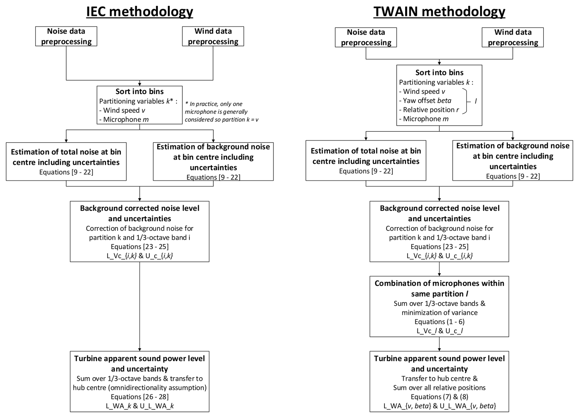
Figure 11 Comparison of data reduction procedure methodology developed in the IEC noise measurement standard (IEC, 2012) (left) and the new methodology proposed for the TWAIN experimental campaign (right). Numbers in brackets [.] refer to equations of the IEC standard, and the ones in parentheses (.) correspond to equations in this paper.

Table 3 List of symbols considered in the data reduction procedure. The first section defines the physical variables used as subscripts, the second the data partition used in the procedure, and the third the acoustic-related quantities calculated. The subscript letter c is taken from the IEC 61400-11-1 standard and refers to the background noise correction.

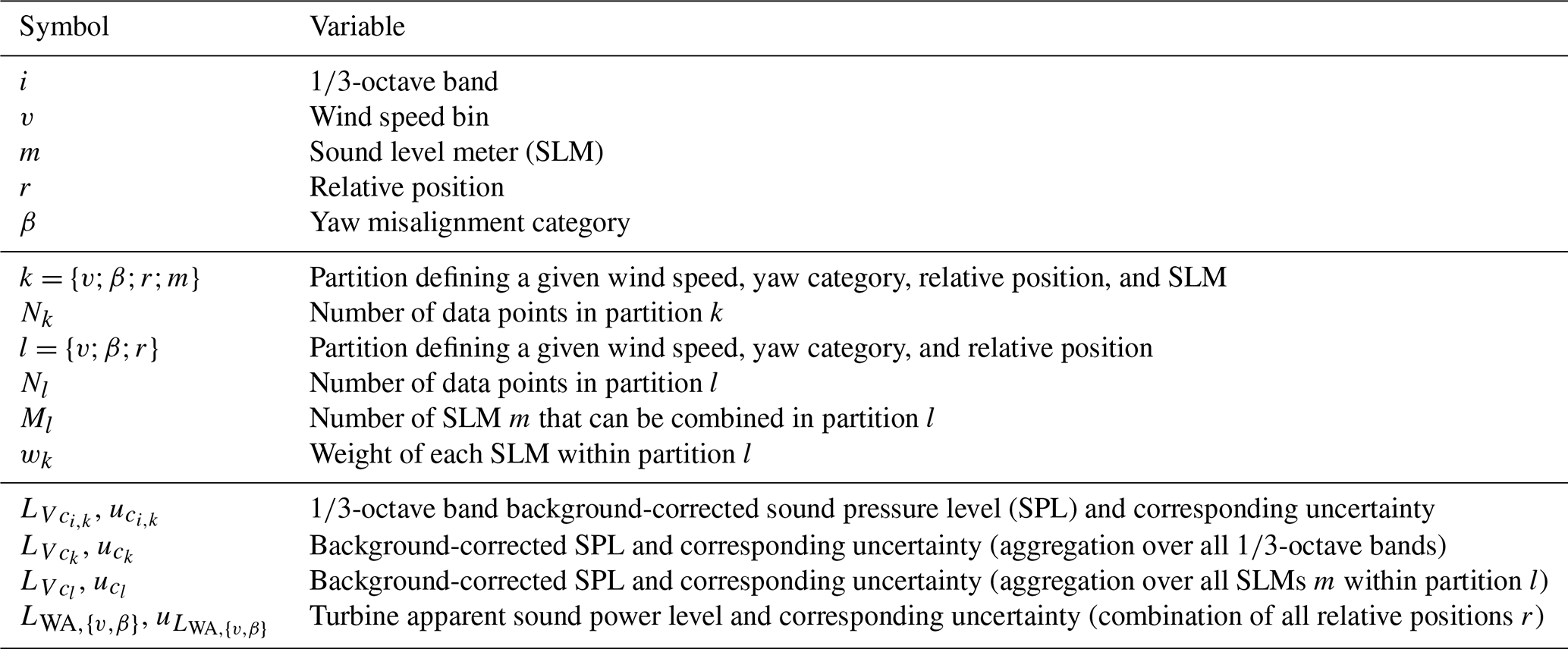
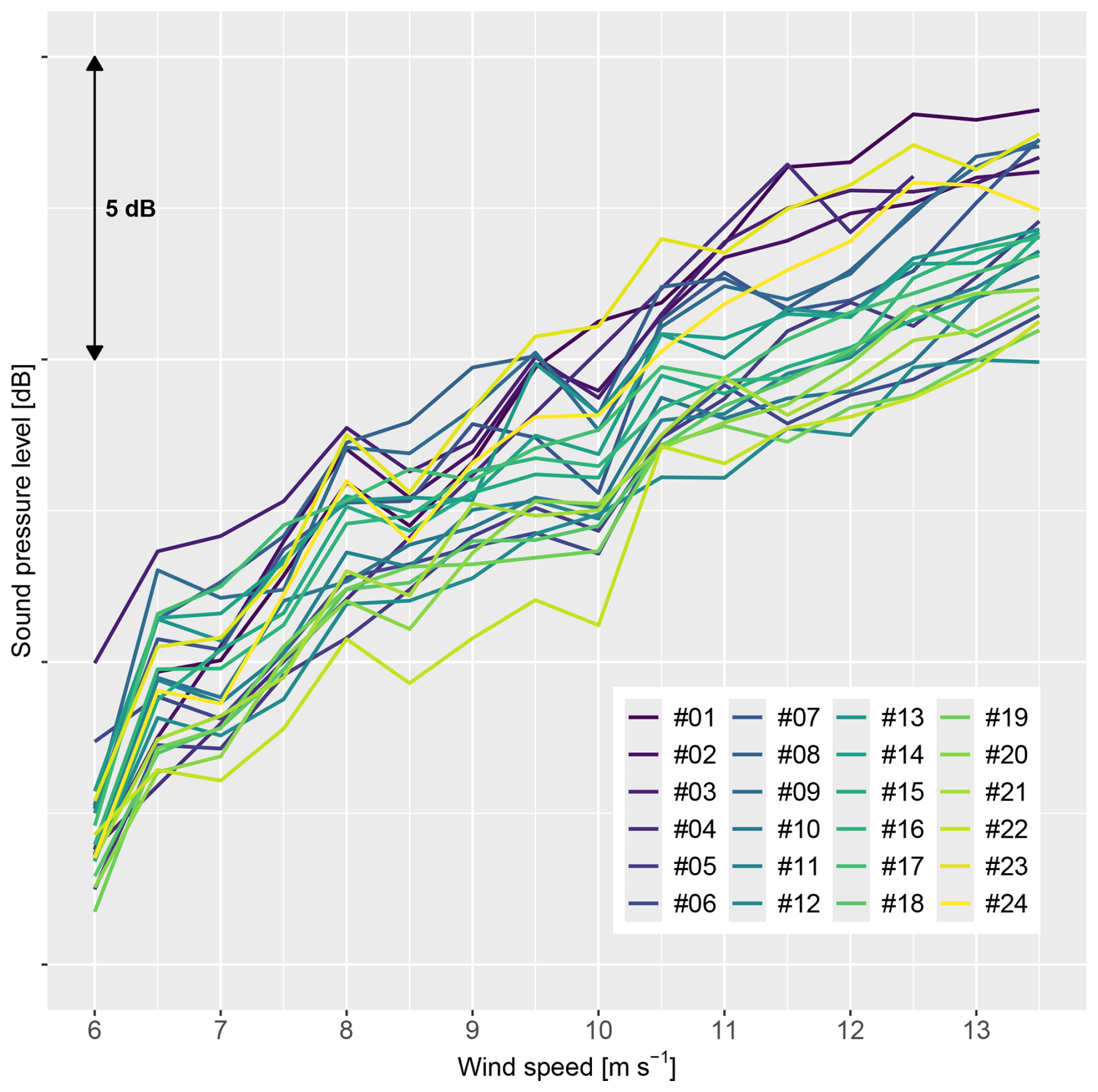
Figure 12 Evolution of median background noise as a function of wind speed bin for each SLM surrounding the wind turbine.

3.3.1 Identification of background noise

The use of 24 SLMs results in as many estimations of background noise. Figure 12 displays the evolution of background noise measured by the 24 sensors as a function of wind speed. All of them show a clear increasing trend with more or less the same slope. However, at a given wind speed, significant differences can be noticed, reaching up to approximately 4 dB when considering the two extreme SLMs. These gaps can be explained by the variety in the local environment around each sensor. For example, SLMs nos. 1 to 12 – located on the southern section of the circle (see Fig. 2) – tend to display a higher background noise than the others: this could be related to the presence of a highway situated approximately 1 km south of the wind turbine. SLMs nos. 23 and 24 show higher background noise compared to their symmetrical counterparts nos. 13 and 14: this could be explained by their location being closer to the substation. Differences in crop cutting around each SLM might also have some influence, especially at high wind speeds.

Due to operational constraints and the necessity of fitting all measurements within only 4 d, it was not possible to conduct additional tests to characterize the background noise variations at the site more accurately. Because of the large disparity observed between all SLMs, it was thus not possible to extract a single background noise value valid for all of them as a function of wind speed. Instead, the approach proposed by Hamilton et al. (2021) was followed, with a specific background noise dataset binned by wind speed calculated for each SLM.

3.3.2 Calculation of noise levels

Like the background noise, the total noise dataset is binned by wind speed for each SLM. However, compared to the IEC standard, two additional variables must be taken into account: one is of course the yaw misalignment angle applied to the turbine, and the second is the relative position of the SLM with respect to the wind direction. Indeed, the noise pattern emitted by a turbine is not homogeneous, and depending on the wind direction, the SLM will not measure the same sound pressure level. For each 10 s chunk, the relative position of an SLM was calculated as the difference between the reference wind direction and the azimuth between the turbine and the SLM and rounded to the closest 15° bin. Consequently, it is no longer required to filter data when the wind direction changes by more than 15° as recommended in the IEC standard; the data are simply redispatched between the 24 SLMs of the circle.

Still, the supplementary partitioning added by this new binning variable complexifies the data processing. Due to the curse of dimensionality, with these four binning variables, some bins find themselves very sparsely populated. Accounting at this stage for the minimum number of 10 samples in each bin would discard a very large number of them (approximately 45 %). Alternatively, to retain as much data as possible, a much smaller value of three samples per bin was used. Note that this reduction is a temporary adjustment. It will be compensated for later in the procedure by imposing a minimum of 10 cumulative samples across SLMs for each set point (wind speed bin, relative position, and yaw angle).

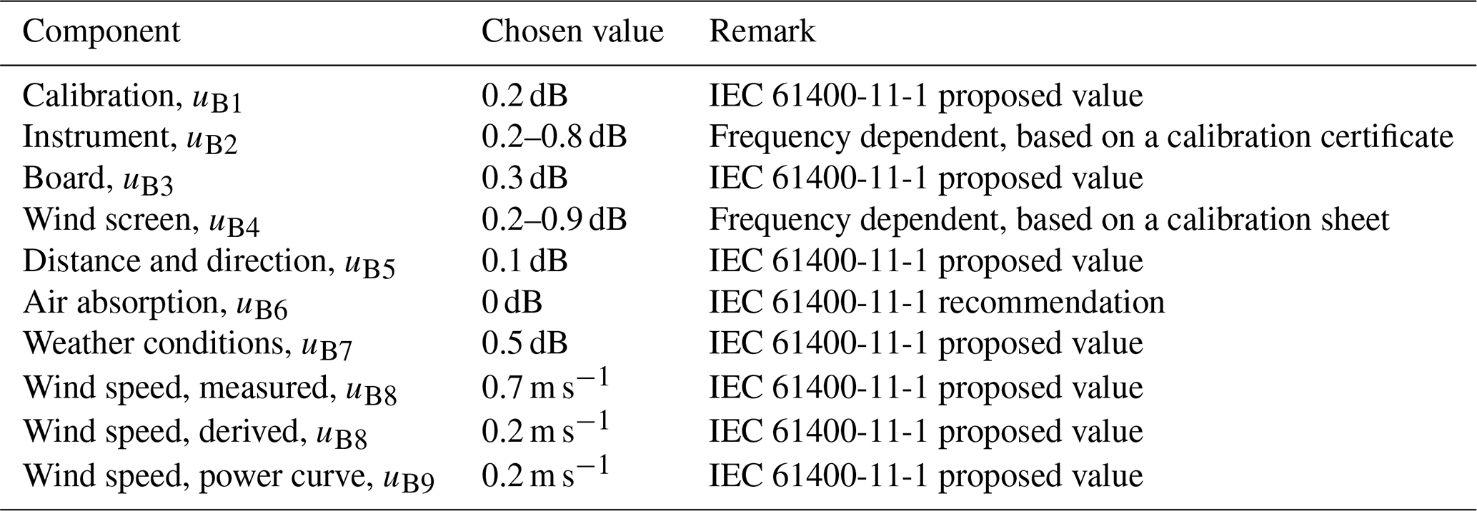
The formula of the IEC noise standard was then applied to every bin in order to calculate the average wind speed and sound pressure level in each $\mathrm{1}/\mathrm{3}$-octave band, evaluate the corresponding uncertainties and covariance, and interpolate the noise levels at the bin center (including uncertainties). Table 4 summarizes the values that were taken for the type B uncertainties. It must be noted that an additional source of uncertainty can arise from the assessment of the turbine yaw misalignment and the slow reaction of its controller to wind direction changes (McKay et al., 2014). However, this error is not listed in the IEC noise standard and therefore not considered in this paper.

Table 4 Type B measurement uncertainties.

Next, the binned total noise is compared to the binned background noise for each SLM. Again, the process indicated by the standard was followed to obtain the background-corrected sound pressure level at the bin center for each $\mathrm{1}/\mathrm{3}$-octave band i within each partition of wind speed v, SLM m, relative position r, and yaw misalignment angle β. The number of samples N_k associated with each partition k (where $k=\mathit{\{}v;\mathit{\beta };r;m\mathit{\}}$) is taken as the lowest number of samples between the total noise and background noise datasets.

The end of the data reduction procedure differs from the one developed in the standard. Rather than calculating the sound power level for each $\mathrm{1}/\mathrm{3}$-octave band, the background-corrected overall A-weighted sound pressure level (OASPL) $L_{V{c}_k}$ is calculated for each k by energy summing all $\mathrm{1}/\mathrm{3}$-octave band background-corrected sound pressure values $L_{V{c}_{i,k}}$.

$$\begin{array}{}\text{(1)}& L_{V{c}_k}=\mathrm{10}\cdot \log \left(\sum _{i=\mathrm{1}}^{\mathrm{28}}{\mathrm{10}}^{\left(\frac{L_{V{c}_{i,k}}}{\mathrm{10}}\right)}\right)\end{array}$$

For SLMs with missing $\mathrm{1}/\mathrm{3}$-octave bands, the measured OASPL was used directly. For those with incomplete $\mathrm{1}/\mathrm{3}$-octave bands, the energy summation was done on the available bands, given that they were previously normalized to match the measured overall sound pressure level. The uncertainty $u_{c_k}$ associated with the obtained OASPL is deduced from the uncertainty in each $\mathrm{1}/\mathrm{3}$-octave pressure value $u_{c_{i,k}}$:

$$\begin{array}{}\text{(2)}& u_{c_k}={\displaystyle \frac{{\sum }_{i=\mathrm{1}}^{\mathrm{28}}{u}_{c_{i,k}}{\mathrm{10}}^{\left(\frac{L_{V{c}_{i,k}}}{\mathrm{10}}\right)}}{{\sum }_{i=\mathrm{1}}^{\mathrm{28}}{\mathrm{10}}^{\left(\frac{L_{V{c}_{i,k}}}{\mathrm{10}}\right)}}}.\end{array}$$

Finally, the OASPLs calculated for several SLMs for the same wind speed, relative position, and yaw category are combined into a single value. This is done by computing a weighted average of $L_{V{c}_k}$ values over all SLMs within the same partition $l=\mathit{\{}v;\mathit{\beta };r\mathit{\}}$:

$$\begin{array}{}\text{(3)}& L_{V{c}_l}=\mathrm{10}\cdot \log \left({\displaystyle \frac{{\sum }_{m=\mathrm{1}}^{M_l}{w}_k{\mathrm{10}}^{\left(\frac{L_{V{c}_k}}{\mathrm{10}}\right)}}{{\sum }_{m=\mathrm{1}}^{M_l}{w}_k}}\right)\end{array}$$

with the corresponding uncertainty

$$\begin{array}{}\text{(4)}& u_{c_l}=\sqrt{{\displaystyle \frac{\mathrm{1}}{{\sum }_{m=\mathrm{1}}^{M_l}{w}_k}}},\end{array}$$

where M_l is the total number of SLMs in the partition l, and the weights w_k are chosen to minimize the variance of the derived estimator (Shahar, 2017):

$$\begin{array}{}\text{(5)}& w_k={\displaystyle \frac{\mathrm{1}}{u_{c_k}^{\mathrm{2}}}}.\end{array}$$

The total number of samples associated with the partition l is simply the sum of samples for all partitions k:

$$\begin{array}{}\text{(6)}& N_l=\sum _{m=\mathrm{1}}^{M_l}{N}_k.\end{array}$$

Only the partitions with N_l≥10 are kept for the end of the analysis. Thus, it fulfills the IEC constraint that at least 10 samples must be present in each bin, with the exception that samples are allowed to come from multiple sensors to keep as much data as possible. With the applied process, SLMs with the lowest uncertainty $u_{c_k}$ (generally because they have more samples in their partition) will have a stronger weight w_k and will contribute more to the derived OASPL value.

3.3.3 Aggregation from noise levels to turbine apparent sound power level

Once the sound pressure values have been obtained for each relative position, they can be aggregated together to derive the turbine apparent overall A-weighted sound power level (OASWL) for each wind speed and yaw position $L_{\mathrm{WA},\mathit{\{}v,\mathit{\beta }\mathit{\}}}$. While sound pressure level (SPL) is a local quantity that quantifies the noise level at a specific point in space possibly arising from many noise sources, sound power level (SWL) quantifies the acoustic energy flux radiated into the atmosphere in all directions from a specific source. Sound power is fundamentally linked to the surface integration of the squared sound pressure field around a source of interest. The term overall is related to the integration of all acoustic frequency components, typically between 20 Hz and 20 kHz.

In contrast to the IEC standard that considers a single SLM located downstream with an omnidirectionality assumption for the noise emission, this novel experimental setup allows for more finesse by accounting for the azimuthal dependence in the estimation of acoustic power. The single contributions at each relative position around the turbine are energy summed, with the hypothesis that the acoustic level is constant over a slice of the hemisphere with an area $\mathrm{4}\mathit{\pi }{R}_{\mathrm{1}}^{\mathrm{2}}\mathit{\tau }$, where R₁=161.1 m is the average distance between all SLMs and the rotor center, and $\mathit{\tau }=\mathrm{1}/\mathrm{24}$ is the angular slice ratio associated with each relative position r. This yields the following equations for $L_{\mathrm{WA},\mathit{\{}v,\mathit{\beta }\mathit{\}}}$ and its respective uncertainty $u_{L_{\mathrm{WA},\mathit{\{}v,\mathit{\beta }\mathit{\}}}}$ (Finez et al., 2025):

$$\begin{array}{}\text{(7)}& {\displaystyle }{L}_{\mathrm{WA},\mathit{\{}v,\mathit{\beta }\mathit{\}}}=\mathrm{10}\cdot \log \left(\sum _{r=\mathrm{1}}^{\mathrm{24}}{\mathrm{10}}^{\left(\frac{L_{V{c}_l}-\mathrm{6}}{\mathrm{10}}\right)}{\displaystyle \frac{\mathrm{4}\mathit{\pi }{R}_{\mathrm{1}}^{\mathrm{2}}}{S_{\mathrm{0}}}}\mathit{\tau }\right),\text{(8)}& {\displaystyle }{u}_{L_{\mathrm{WA},\mathit{\{}v,\mathit{\beta }\mathit{\}}}}={\displaystyle \frac{{\sum }_{r=\mathrm{1}}^{\mathrm{24}}{u}_{c,l}{\mathrm{10}}^{\left(\frac{L_{V{c}_l}-\mathrm{6}}{\mathrm{10}}\right)}\frac{\mathrm{4}\mathit{\pi }{R}_{\mathrm{1}}^{\mathrm{2}}}{S_{\mathrm{0}}}\mathit{\tau }}{{\sum }_{r=\mathrm{1}}^{\mathrm{24}}{\mathrm{10}}^{\left(\frac{L_{V{c}_l}-\mathrm{6}}{\mathrm{10}}\right)}\frac{\mathrm{4}\mathit{\pi }{R}_{\mathrm{1}}^{\mathrm{2}}}{S_{\mathrm{0}}}\mathit{\tau }}},\end{array}$$

where S₀=1 m² is a reference area. A linear interpolation from adjacent observer positions r is operated in the case of missing $L_{V{c}_l}$ values due to a lack of measurement data. If more than 4 points out of the 24 positions were missing for a given wind speed and yaw misalignment category, the corresponding OASWL value was not calculated.

With Eq. (7), the effect of yaw misalignment on turbine apparent sound power can be properly estimated, without being biased by the rotation of the noise directivity pattern, as will be discussed in the next section.

4 Results and discussion

Following the data processing methodology described in Sect. 3, noise directivity patterns are calculated on the measurement data and presented in this section. In order to harmonize the results coming from multiple wind directions, the sign conventions defined in Fig. 13 are adopted. First, in Sect. 4.1, turbine noise emissions are analyzed when they are aligned with the wind. The effect of yaw misalignment is then compared to the yaw-aligned situation in Sect. 4.2.

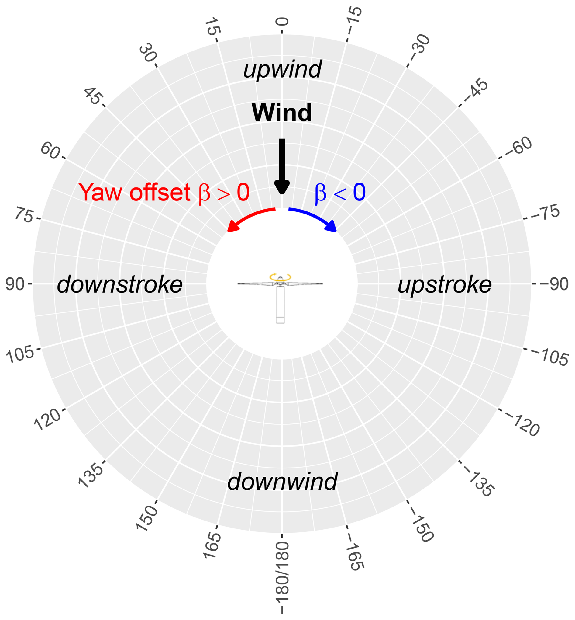
Figure 13 Sign convention followed for the display of the directivity patterns as a function of the observer angle θ. Wind direction always comes from the angle θ=0°, while $\mathit{\theta }=-\mathrm{180}\mathit{°}/\mathrm{180}\mathit{°}$ is the downwind position. Positive yaw angles β are defined as a counter-clockwise rotation of the nacelle when seen from above. Positive and negative relative positions correspond to the downstroke and upstroke sides of the rotor plane, respectively.

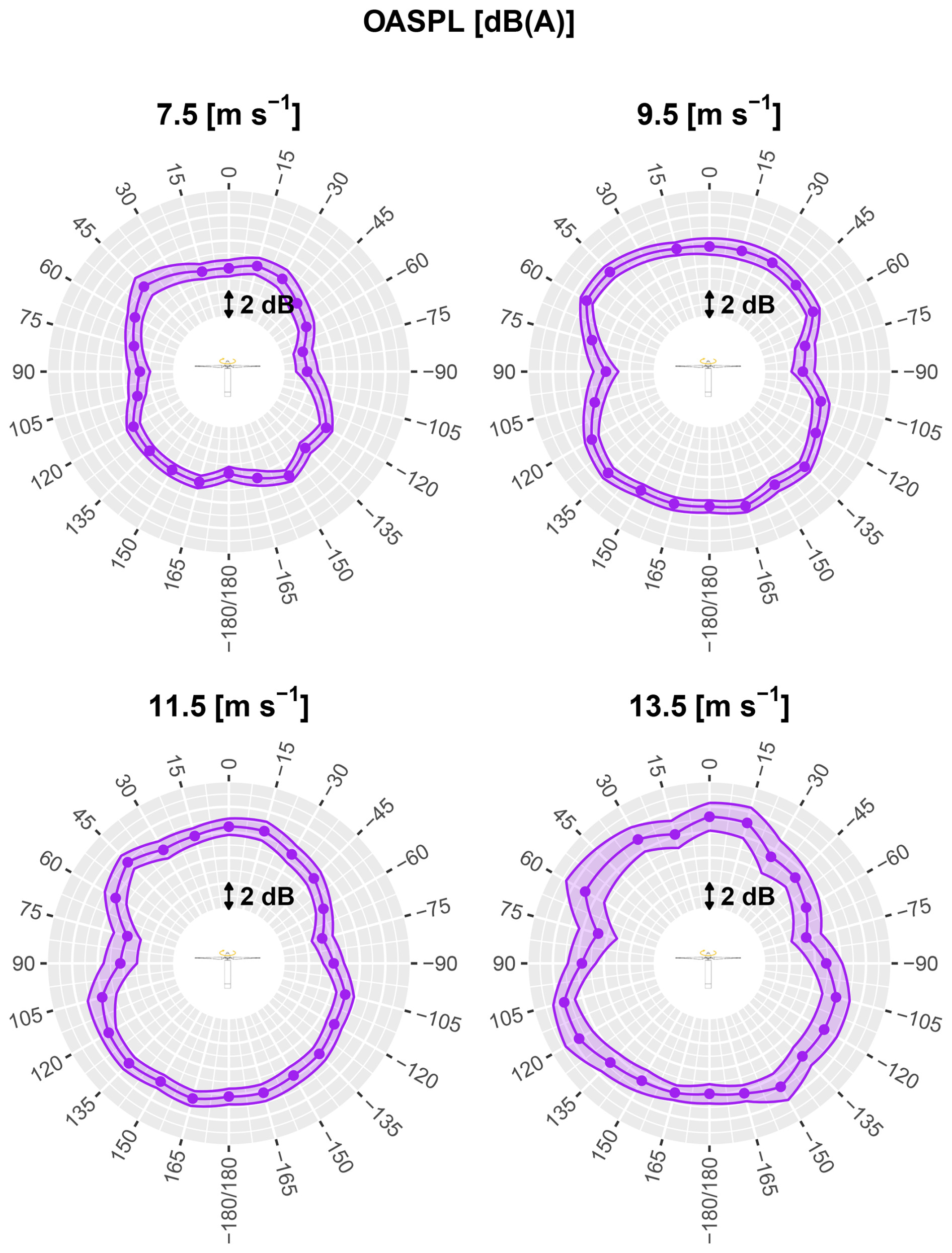
Figure 14 Directivity of overall A-weighted sound pressure level (OASPL) for four different wind speeds. In each graph, the wind comes from the top (position 0°), and positive and negative angles correspond to the downstroke and upstroke sides of the rotor, respectively. The shaded ribbon represents 1 standard uncertainty associated with each OASPL value $u_{c_l}$, while the point markers indicate the mean value $L_{V{c}_l}$. For observer positions containing fewer than 10 valid samples, the corresponding data point is omitted.

4.1 Directivity of turbine noise emissions with no misalignment

The OASPLs of the estimated turbine noise are presented in Fig. 14 for each observer position relative to the nacelle axis without yaw misalignment and across four wind speed bins. Since the turbine reaches rated power at 12 m s⁻¹, the selected wind speeds correspond to 52 % to 100 % of rated power. At all observed wind speeds, OASPL variations in the ground-based directivity pattern reach up to 4 dB(A). In each plot, a region of low noise levels is observed near the rotor plane, sometimes referred to as “noise dips” in the literature (Oerlemans and Schepers, 2009). Within these dips, sound levels are consistently 3.5 to 4.0 dB(A) lower than the maximum values in the corresponding directivity pattern. At lower speeds (7.5 and 9.5 m s⁻¹), the minimum noise levels occur at observer angles of $\mathit{\theta }=\pm \mathrm{90}\mathit{°}$. Interestingly, near rated power (11.5 and 13.5 m s⁻¹), the noise dips shift upstream, appearing at $\mathit{\theta }=\pm \mathrm{75}\mathit{°}$.

The direction of the maximum noise level is not aligned with the downstream flow axis but rather occurs at off-axis positions, either upstream or downstream of the turbine. Specifically, the peak noise levels are observed at $\mathit{\theta }=-\mathrm{150}\mathit{°}$ at 7.5 m s⁻¹, θ=135° at 9.5 m s⁻¹, θ=45° at 11.5 m s⁻¹, and θ=120° at 13.5 m s⁻¹. These levels exceed the axial downstream measurement by 1.4, 0.7, 0.8, and 1.6 dB(A), respectively. This observation is not captured by most existing analytical and semi-empirical models (Bertagnolio et al., 2023), which typically predict symmetric directivity patterns with the maximum aligned along the main flow axis. In contrast, the directivity patterns shown in Fig. 14 exhibit slight asymmetries with respect to not only the nacelle axis, but also the rotor plane. Since the observed differences in noise levels remain within the uncertainty bounds, a statistical paired t test was conducted to support this visual observation. The test is based on the level difference between two symmetrical positions $\mathrm{\Delta }{L}_{V,\mathit{\theta }}=L_{V,\mathit{\theta }}-L_{V,{\mathit{\theta }}^{\prime }}$ for the same wind speed bin, where θ^′ is chosen as

• ${\mathit{\theta }}^{\prime }=-\mathit{\theta }$ to test the down-upstroke symmetry and

• ${\mathit{\theta }}^{\prime }=\mathrm{90}\mathit{°}-\mathit{\theta }$ to test the down-upwind symmetry.

The set of available observation angle pairs $(\mathit{\theta };{\mathit{\theta }}^{\prime })$ is denoted as Θ and consists of 207 observations in both of the above-mentioned cases. The level difference ΔL_V,θ is associated with a combined variance $u_{\mathit{\theta }}^{\mathrm{2}}$ such as

$$\begin{array}{}\text{(9)}& u_{\mathit{\theta }}^{\mathrm{2}}=u_{c,\mathit{\theta }}^{\mathrm{2}}+u_{c,{\mathit{\theta }}^{\prime }}^{\mathrm{2}}-\mathrm{2}\mathit{\rho }{u}_{c,\mathit{\theta }}{u}_{c,{\mathit{\theta }}^{\prime }},\end{array}$$

where ρ is the correlation factor between the θ and θ^′ series, which may be non-zero due to the previously identified noise dips. Following the approach in Eqs. (3)–(5), the weights are defined as the inverse of the combined variance $w_{\mathit{\theta }}=\mathrm{1}/u_{\mathit{\theta }}^{\mathrm{2}}$, and the weighted average of the level difference is computed as

$$\begin{array}{}\text{(10)}& {\stackrel{\mathrm{‾}}{\mathrm{\Delta }L}}_V={\displaystyle \frac{{\sum }_{\mathit{\theta }\in \mathrm{\Theta }}{w}_{\mathit{\theta }}\mathrm{\Delta }{L}_{V,\mathit{\theta }}}{{\sum }_{\mathit{\theta }\in \mathrm{\Theta }}{w}_{\mathit{\theta }}}}\end{array}$$

with the standard error

$$\begin{array}{}\text{(11)}& {\mathit{\sigma }}_{\mathrm{\Delta }L}=\sqrt{{\displaystyle \frac{\mathrm{1}}{{\sum }_{\mathit{\theta }\in \mathrm{\Theta }}{w}_{\mathit{\theta }}}}}.\end{array}$$

This enables us to use the test statistics $t={\stackrel{\mathrm{‾}}{\mathrm{\Delta }L}}_V/{\mathit{\sigma }}_{\mathrm{\Delta }L}$, which are applied across the full set of available wind speed bins at once using a significance level of 5 % and assuming a normal distribution. On average, the OASPL value on the downstroke side is found to be 0.6 dB higher than on the upstroke side. The 95 % confidence interval is [0.5; 0.8] dB, associated with a p value $p<{\mathrm{10}}^{-\mathrm{6}}$, indicating a highly significant left–right asymmetry in the directivity pattern. This result was found to be virtually independent of the correlation factor ρ within the range 0 to 0.5.

The same approach was applied to assess the symmetry between downwind and upwind directions. On average, the sound level measured on the downwind side was 0.4 dB higher than that on the upwind side at observer positions symmetric with respect to the rotor plane. The 95 % confidence interval for this difference is [0.3; 0.6] dB(A), associated with a p value $p<{\mathrm{10}}^{-\mathrm{8}}$, again indicating a highly significant asymmetry.

From this analysis, it can be concluded that the directivity footprint of the turbine exhibits, on average, 0.6 dB(A) higher noise levels on the downstroke side compared to the upstroke side and 0.4 dB(A) higher levels on the downwind side compared to the upwind side. These slight asymmetries in the turbine’s noise radiation may result from the intrinsic directivity of elementary acoustic sources. Analytical models based on flat-plate assumptions (as for instance Tian and Cotté, 2016) and (semi-)empirical models derived from symmetric airfoil measurements (Bertagnolio et al., 2023) do not reproduce such asymmetries. However, camber has been shown to cause deviations of up to 1 dB(A) between the pressure and the suction side noise radiation of a nonsymmetrical airfoil (Roger and Moreau, 2010). This behavior has also been captured in high-fidelity numerical simulations of cambered and loaded airfoils equipped with serrations (Romani et al., 2021). Thus, the turbine blade camber may be responsible for an asymmetric radiation on both sides of the airfoils. As the chord line is more or less contained in the rotation plane, it may result in an upstream–downstream asymmetry in noise levels at the turbine level. The left–right asymmetry is more likely to be linked to both the trailing-edge noise directivity and the acoustic amplification term as already proposed by Oerlemans et al. (2007).

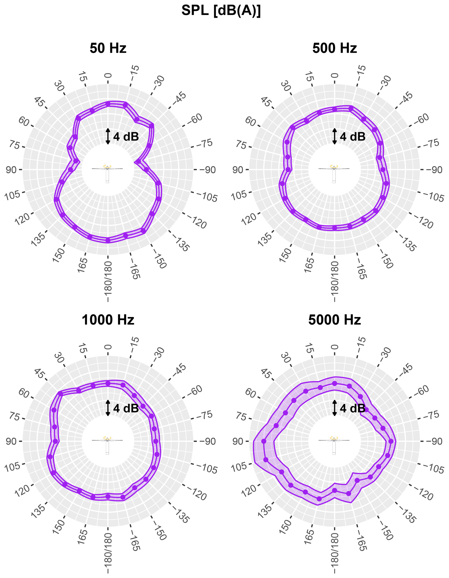
Figure 15 Directivity of A-weighted sound pressure level (SPL) at 11.5 m s⁻¹ for four different $\mathrm{1}/\mathrm{3}$-octave bands without yaw misalignment. The shaded ribbon represents 1 standard uncertainty.

Spectral directivity patterns at near-rated power (11.5 m s⁻¹) are presented in Fig. 15 over a selected frequency range. At very low frequencies (e.g., 50 Hz), the pattern exhibits two distinct lobes oriented upstream and downstream, with higher levels on the downstream side. Pronounced noise dips are also observed, with sound levels up to 6 dB lower than at the axial downwind position, which corresponds to the direction of maximum noise emission at this frequency. As frequency increases, the directivity pattern becomes more complex, featuring several off-axis lobes. For instance, in the mid-frequency range of around 1000 Hz – where human hearing is most sensitive – a narrow lobe centered at θ=45° emerges, with noise levels approximately 4 dB higher than at adjacent directions. A secondary, less pronounced lobe appears on the descending blade side around θ=120°. These features are also reflected in the OASPL directivity patterns (lower-left part of Fig. 14) at θ=45 and θ=135°. At higher frequencies (e.g., 5000 Hz), the pattern displays multiple lobes with significant local variations and increased uncertainty (±2.0 dB) compared to lower frequencies. This uncertainty increase is due to a higher data dispersion at 5 kHz than at lower frequencies (“type A” component).

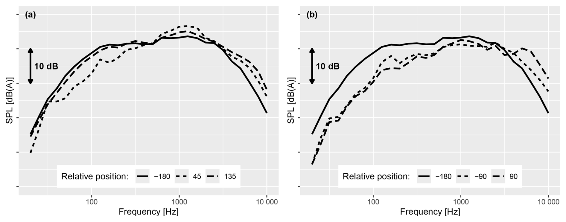
Figure 16 Noise spectra measured at 11.5 m s⁻¹. The sound pressure level (SPL) is represented for different positions of the circle. On the left (a), spectra at the two lobes of the directivity pattern (45° for the upstream lobe, 135° for the downstream) are compared to the spectrum at the central downstream location (180°). On the right (b), spectra in the rotor plane (90° for upstroke, −90° for downstroke) are compared to the downstream location (180°). The y axes are consistent between the two panels.

A complementary perspective is provided in Fig. 16, which compares frequency spectra at selected observer positions. In Fig. 16a the maxima of the two OASPL lobes at 11.5 m s⁻¹ – located at θ=45 and θ=135° – are compared to the reference axial downstream position (θ=180°). At these two positions, the spectral content shows a pronounced mid-frequency component between 800 and 2000 Hz with increases of 5 and 3 dB, respectively, relative to the reference. At the very high frequency range (above 5000 Hz), further increases of +7 and +5 dB are observed. Conversely, a reduction in the low-frequency range (50–500 Hz) is noted, particularly at θ=45°, where levels are 7 dB(A) lower than at the reference.

Figure 16b presents two additional measurement points at the same wind speed, comparing positions in the rotor plane to the axial downwind reference. In the noise dip regions, the low-frequency content is significantly reduced – by up to 10 dB at 100 Hz. In contrast, an increase in the very high frequency range is observed, especially on the descending blade side (θ=90°). In summary, at this specific wind speed, the spectral analysis reveals a strong broadband component in the mid-frequency range at off-axis lobe maxima, as well as a spectral shift toward higher frequencies in the noise dip regions, relative to the axial downwind position.

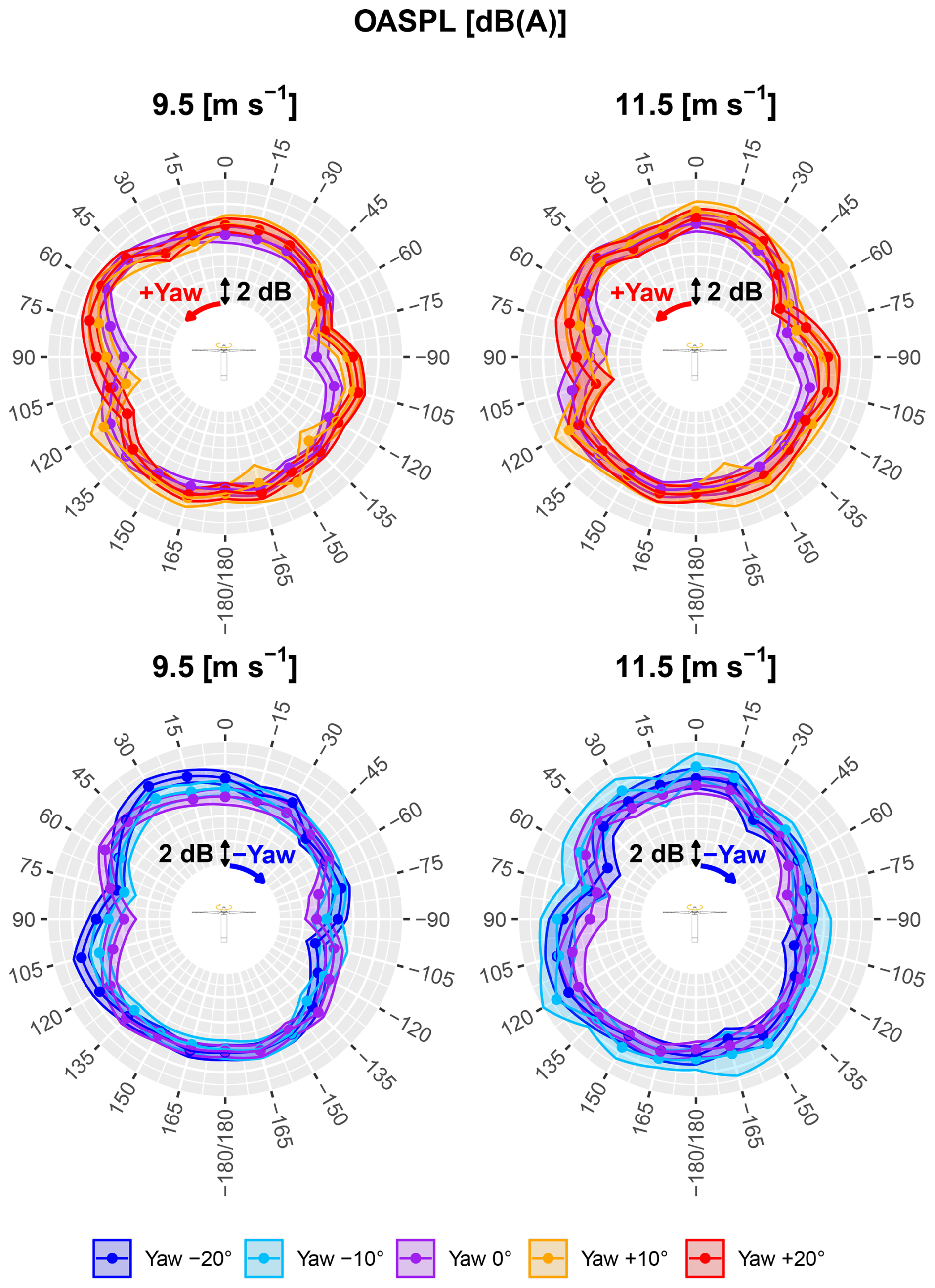
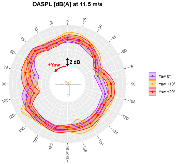
Figure 17 Directivity of overall A-weighted sound pressure level (OASPL) for positive (top) and negative (bottom) yaws and two different wind speeds. In each graph, the wind comes from the top (position 0°), and positive and negative angles correspond to downstroke and upstroke sides of the rotor, respectively. The shaded ribbon represents 1 standard uncertainty associated with each OASPL value $u_{c_l}$, while the point markers indicate the mean value $L_{V{c}_l}$. For observer positions containing fewer than 10 valid samples, the corresponding data point is omitted.

4.2 Effect of yaw misalignment

Directivity patterns under intentional yaw misalignment are illustrated in Fig. 17 at 9.5 and 11.5 m s⁻¹. The first row shows positive yaw misalignment angles (i.e., the ascending blade is oriented toward the incoming flow), while the second row presents negative yaw misalignment angles (i.e., the ascending blade is oriented away from the flow). A first observation is that yaw misalignment does not lead to dramatic changes in overall noise levels. The most prominent effect of steering the turbine away from the main flow direction is a rotation of the entire directivity pattern, which appears to remain aligned with the turbine orientation in all four cases – particularly around the recognizable noise dip regions. It is worth noting that the yaw angle sampling step Δβ=10° is not a multiple of the observer angle sampling step Δθ=15°, which explains why the noise dips may appear at similar positions for different yaw angles. Some regions appear to be more strongly influenced by the flow direction than by the turbine orientation and are amplified when a yaw misalignment is applied. This is particularly evident in the upwind-upstroke sector [0°; −45°] for β>0 and in the upwind-downstroke sector [0°; +45°] for β<0. In general, larger absolute yaw misalignment angles β tend to introduce greater complexity into the directivity pattern.

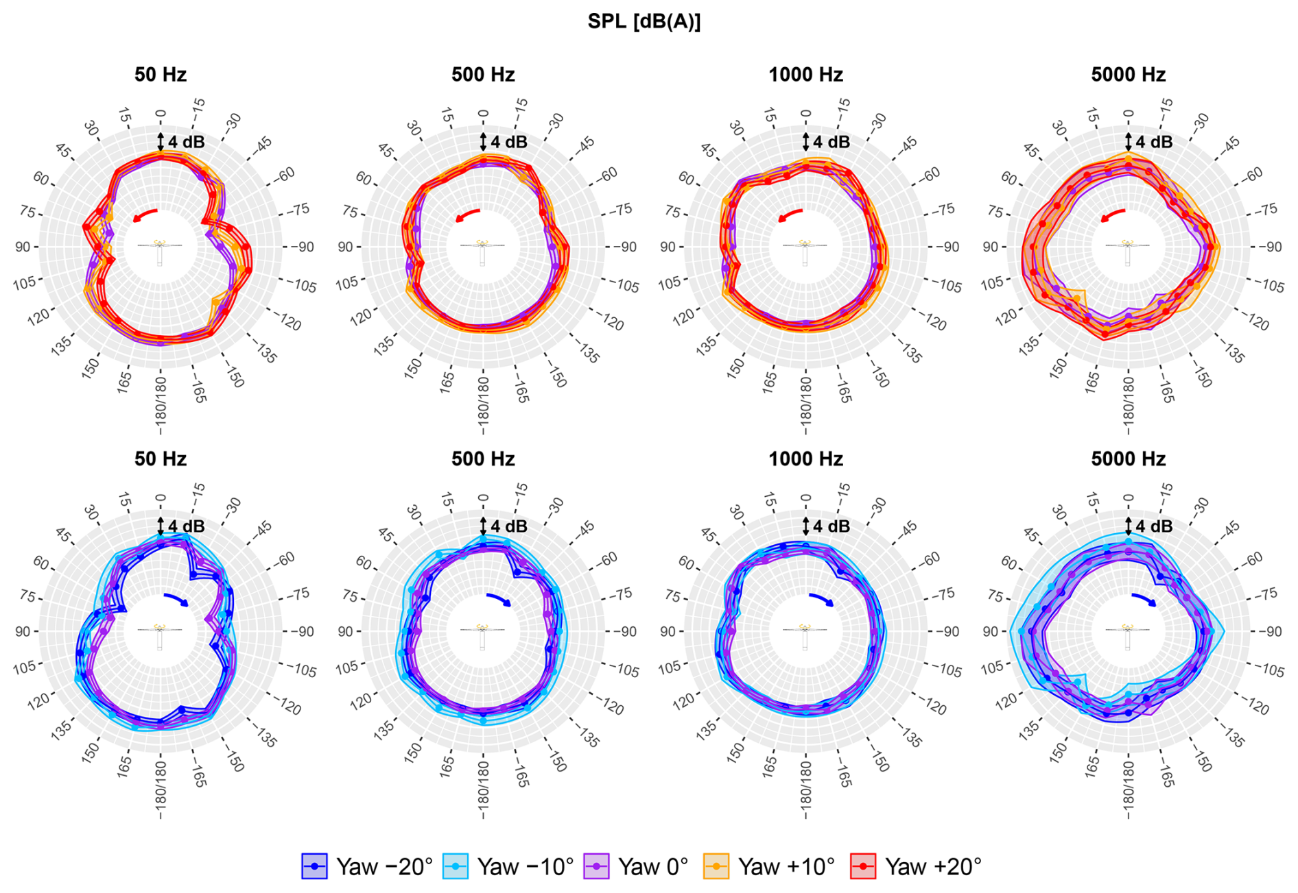
Figure 18 Directivity of A-weighted sound pressure level (SPL) at 11.5 m s⁻¹ for positive (top) and negative (bottom) yaw angles and four different $\mathrm{1}/\mathrm{3}$-octave bands. The shaded ribbon represents 1 standard uncertainty.

Spectral variations in the directivity patterns at v=11.5 m s⁻¹ are illustrated in Fig. 18. At the lowest frequencies (50 Hz), the rotation of the directivity pattern induced by the turbine misalignment is particularly visible. The most significant variations with respect to the yaw misalignment angle β are predominantly localized near the rotor plane ($\left|\mathit{\theta }\right|\simeq \mathrm{90}\mathit{°}$). However, the acoustic impact of yaw misalignment in the lowest frequency range (50 Hz) cannot be reduced to a rotation. The simple two-lobe pattern of the aligned case cannot be recognized at other yaw angles, showing a more complex structure. It may be the expression of a significant change in the prominent aeroacoustic sources at this frequency. Interestingly, this is not the case for most of the other plots at higher frequencies in Fig. 18. It is generally accepted that wind turbine aerodynamic noise is dominated by the turbulent boundary layer–trailing-edge noise (TBL-TE) in the higher-frequency range, typically above 800 Hz, and by the turbulent inflow (TI) noise at lower frequencies. If this holds for the current turbine, it would suggest that the yaw misalignment has a strong influence on the TI component and virtually not on the TBL-TE component, at least up to 5 kHz. TI noise is produced by the interaction between turbulent eddies in the atmosphere with the moving leading edge of the three blades. In yaw-aligned conditions, a scaling variable of TI noise models is the integral length scale of the atmospheric turbulence. The phase relationship between the relative normal wind velocity component encountered by different sections of a blade is indeed important, as it can reinforce or mitigate the noise production process. A typical signature of this relationship at the airfoil level is its noise directivity pattern. As the turbine is yawed, the blades pass through atmospheric turbulence with an angle. With the turbulence longitudinal correlation, this angle may increase the apparent length scale and reinforce the TI noise production process and alter its directivity trace on ground SLMs. Conversely, TBL-TE noise is produced by the interaction of a turbulent boundary layer (at the surface of the blade) and the trailing edge. The process is somewhat more local and may be less influenced by the yaw configuration.

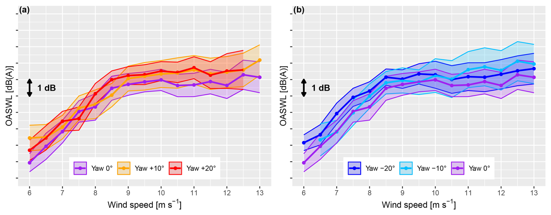
Figure 19 Turbine overall A-weighted sound power level (OASWL) as a function of wind speed for positive (a) and negative (b) yaws. The shaded ribbon represents 1 standard uncertainty associated with each OASWL value $u_{L_{\mathrm{WA},\mathit{\{}v,\mathit{\beta }\mathit{\}}}}$, while the point markers indicate the mean value $L_{\mathrm{WA},\mathit{\{}v,\mathit{\beta }\mathit{\}}}$. For wind speed bins and yaw misalignment cases with observer positions that are too few, the point is omitted.

Estimates of the turbine's OASWL derived using Eqs. (7) and (8) are presented in Fig. 19 for various yaw misalignment angles, both positive (left panel) and negative (right panel). All empirical sound power curves exhibit a consistent structure, characterized by a linear increase between 6 and 9 m s⁻¹, followed by a plateau at higher wind speeds, as expected for this turbine. For most wind speed bins, the aligned configuration β=0° is the less noisy configuration. In contrast, configurations with yaw misalignment tend to exhibit more elevated sound power levels. To evaluate the statistical significance of these observations, four inverse-variance-weighted paired t tests were conducted using Eqs. (10) and (11). Each test compares the sound power curve for a misaligned configuration $L_{\mathrm{WA},\mathit{\{}v,\mathit{\beta }\ne \mathrm{0}\mathit{°}\mathit{\}}}$ against the reference aligned configuration $L_{\mathrm{WA},\mathit{\{}v,\mathit{\beta }=\mathrm{0}\mathit{°}\mathit{\}}}$. The results, summarized in Table 5, indicate that for yaw angles of $\mathit{\beta }=-\mathrm{20}$, +10, 20°, the differences are statistically significant (p<0.05). These configurations exhibit a consistent increase in OASWL of approximately 0.5 to 0.7 dB(A). Accordingly, it can be concluded that these misaligned settings are slightly noisier than the baseline configuration, with an average increase in sound power of approximately 0.6 dB(A).

Table 5 The t test results for the offset in sound power level curves compared to the aligned case.

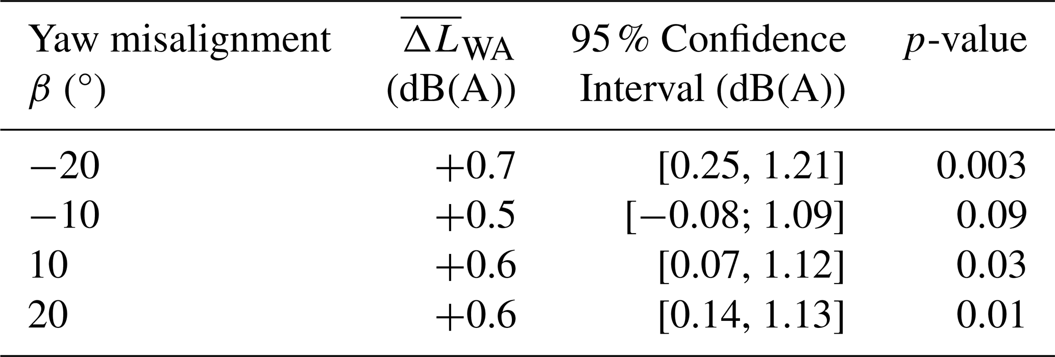
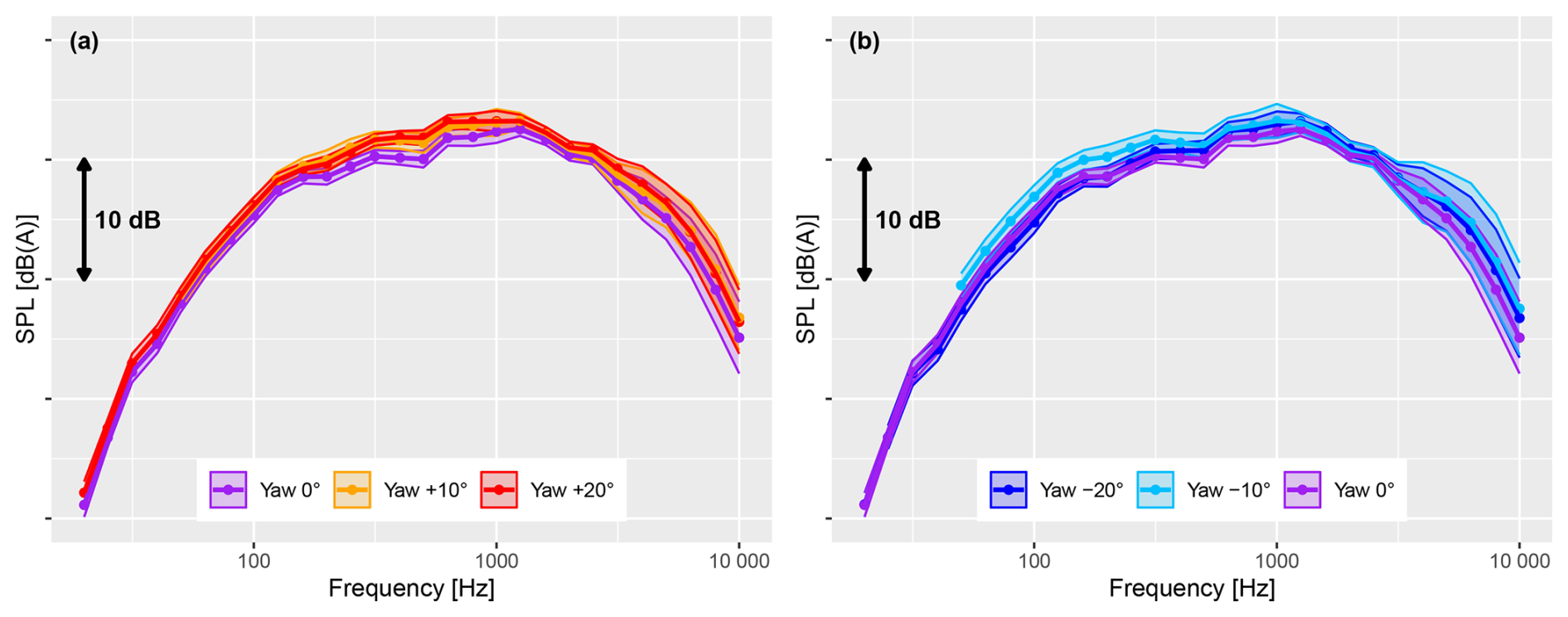
Figure 20 Turbine sound power level spectra at v=11 m s⁻¹ for positive (a) and negative (b) yaw angles. The shaded ribbon represents 1 standard uncertainty.

The slice summation described in Eq. (7) can be independently computed for each $\mathrm{1}/\mathrm{3}$-octave band, yielding the turbine's sound power level spectra. These spectra are presented in Fig. 20 for various yaw misalignment configurations. Consistent with the OASPL analysis, all yaw-misaligned configurations exhibit higher spectral levels compared to the baseline (aligned) case. The increase is particularly notable in the low- to mid-frequency range (200–1250 Hz), as well as in the high-frequency range (f>5 kHz). As previously discussed in the analysis of Fig. 18, this pattern suggests that the dominant noise generation mechanisms are differentially influenced by turbine yaw misalignment. At the wind farm level, the observed slight increase in TI noise levels under misaligned yaws may be compensated for by the fact that wake–turbine interactions are basically avoided in WFFC control strategies, a situation which typically produces large TI noise increases.

The results presented here may be compared with the extensive noise measurement campaign conducted at NREL by Hamilton et al. (2021) near a 77 m diameter 1.5 MW industrial wind turbine subjected to a yaw misalignment ranging from −18 to +25°. They reported a general decrease in SPL by 2 to 3 dB for intermediate yaw offsets (10 and 18°). At more extreme yaw misalignments of −18 and 25°, even larger noise decreases were observed, reaching up to −5 dB compared to the non-steered configuration. At first glance, this appears to contradict the present study, which reports a slight increase of +0.6 dB in noise power levels under yawed conditions. However, several aspects should be considered before drawing such a conclusion.

First, the turbines under investigation are from different manufacturers, and their designs differ significantly. The rated powers differ by 31 % and the diameters by 30 %, and the blade geometries are also dissimilar. For instance, suction side flow recirculation may occur for one blade design under yaw but not for another, with potentially significant consequences for noise emissions. To date, there is no general evidence supporting the assumption that the effect of wake steering on noise emissions is model independent. More specifically, the turbine controllers¹ under consideration appear to respond differently to the yaw misalignment. Hamilton et al. (2021) noticed a reduction in rotor speed under yawed operation at low and moderate wind speeds v≤10 m s⁻¹, which they identified as the main cause of the observed noise reduction. In contrast, in the present study, no systematic change in rotor speed was observed under yaw misalignment. Therefore, differences in turbine control strategies could plausibly explain why no noise level reduction is observed here. However, this explanation only applies to wind speeds below 10 m s⁻¹, whereas the NREL study reports noise reductions at higher wind speeds as well.

Second, the NREL study was limited to the downstream region with a viewing angle of approximately 100° and an angular resolution of 25°. Under such conditions, variations in measured noise levels cannot be directly attributed to changes in turbine emissions alone, as the rotation of the directivity pattern also plays a role. In particular, SLMs falling in the noise dip – depending on their position and the yaw angle – may record an apparent noise reduction, even if the total turbine noise power remains unchanged. Indeed, in the NREL study, SLMs consistently showing SPL reductions under yaw misalignment were located closer to the rotor plane than in the non-steered configuration. This ambiguity motivated the use of a larger number of SLMs in the present setup, uniformly distributed on a circle centered on the wind turbine.

Finally, it should be noted that the largest noise reduction reported in the NREL study occurs at 25° yaw, a configuration that is not investigated here. Although the amount of data, the wind speed range, and the pre- and post-processing strategies are broadly comparable between the two studies, it is suggested that the differing conclusions arise from differences in turbine control strategies, experimental setups, and yaw misalignment ranges. Another point of comparison is provided by Bonsma et al. (2019). Using two SLMs, they monitored noise levels within a wind farm equipped with six industrial turbines operated under WFFC. They reported no statistically significant difference in the sound levels between the regular and yaw-misaligned operation. While this setup – featuring six steered turbines but only two sensors – is relevant from a wind farm operator's perspective, it is not suitable for detecting small variations in individual turbine noise power levels of the order of 0.5 dB. This limitation again arises because fixed sensors are influenced by both the rotation of the directivity pattern rotation and potentially small variations in noise power, with the latter requiring a larger amount of data and number of sensors to be reliably detected. Finally, both studies from the literature are generally consistent with the present work in indicating that the application of WFFC does not lead to a large increase in sound power emissions that could compromise the objective of enhancing power production.

5 Conclusions

A novel acoustic measurement campaign was conducted around an industrial 2.2 MW wind turbine, involving 24 ground-based sound level meters and multiple lidar devices to monitor incoming wind speed and direction. The experiment encompassed a wide range of wind conditions, enabling the construction of detailed directivity patterns across the turbine's full operational range. Modifications to the IEC standard methodology were proposed to leverage the advantages of this multi-point measurement setup. Furthermore, the turbine was operated both under standard alignment control and with intentional yaw misalignment (angles ranging from −20 to +20°) in order to investigate sound power variations associated with wake steering strategies.

Measurements conducted under non-steered conditions reveal that the turbine generally exhibits a two-lobe directivity pattern aligned with the nacelle axis. However, in most tested configurations, the axial downwind direction does not correspond to the direction of maximum emissivity, with differences ranging from 0.7 to 1.6 dB(A), in contrast to predictions from most semi-empirical and analytical wind turbine noise models. Furthermore, the measured directivity patterns display asymmetry, with a statistically significant offset of +0.6 dB on the downstroke side compared to its symmetrical upstroke counterpart and +0.4 dB on the downwind side relative to the upwind side. Spectral comparisons in the off-axis directions of maximum OASPL ($\mathit{\theta }=+\mathrm{45}$ and $\mathit{\theta }=+\mathrm{135}\mathit{°}$) reveal a pronounced broadband contribution of around 1000 Hz, reduced sound pressure levels at low frequencies, and elevated levels at high frequencies (f>5 Hz).

Acoustic curtailment plans are currently still derived assuming turbines are omnidirectional noise sources. By accounting for a more detailed directivity pattern in the design of those plans, wind farm operators could be able to develop much more refined strategies that could in turn lead to significant energy gains over the full lifetime of a project.

When yaw misalignment is applied, the directivity pattern rotates in alignment with the turbine's axis, exhibiting increased complexity with additional lobes and dips compared to standard operating conditions. An increase in the turbine's sound power level, estimated from the multi-point ground-based acoustic footprint, is observed – approximately +0.6 dB(A), independently of the actual yaw angle value. This increase is particularly pronounced in the low-frequency range (below 1000 Hz) and the high-frequency range (above 5000 Hz), suggesting that yaw misalignment differentially affects the primary noise generation mechanisms.

This first-of-its-kind experiment underlines the complexity of multi-objective WFFC and the need for more detailed analytical noise models. Indeed, while wake steering has shown consistent results in mitigating wake effects and improving overall wind farm production, the increased noise emissions could lead to more restrictive acoustic curtailment plans that will have the opposite effect on farm performance. Reliable models must be developed so that operators can weigh the costs and benefits of their choices and make better-informed decisions. Future work in the scope of the TWAIN project will focus on the validation of more advanced turbine noise emission models using the data generated through this experiment, which will later be used in a case study combining wake steering and noise optimization.