SANDWake3D: a 3D parabolic RANS solver for atmospheric surface layers and turbine wakes

Despite many recent advances, modeling wind turbine wakes using semi-empirical and analytical models still faces challenges when dealing with more complicated situations involving wind shear, veer, atmospheric stratification, and wake superposition. To address these limitations, this study introduces a three-dimensional, parabolic Reynolds-averaged Navier–Stokes (RANS) k−ϵ formulation which includes an atmospheric boundary layer model and an actuator disk model for turbine wakes. The full three-dimensional solution for the velocity, temperature, and turbulence variables is efficiently solved through an alternating-direction implicit scheme that requires orders of magnitude fewer computational resources than traditional high-fidelity approaches, such as fully elliptic RANS or large-eddy simulations (LESs). The results of the parabolic RANS model are compared to the equivalent LES and semi-empirical wake models at different wind speeds under stable atmospheric conditions with veer and shear at a single TI level, as well as a convectively unstable-inflow case. For the single-turbine wake the RANS model was able to capture the wake deficit behavior, including the wake stretching and skewing that was observed in the LES. The distribution of the wake turbulence in the RANS model also agreed with results from the higher-fidelity simulations. In simulations of a two-turbine, directly waked configuration, the new RANS model was able to handle the wake superposition behavior without difficulty and also correctly modeled the corresponding increase in wake turbulence when compared to LES. A demonstration of the RANS model on a nine-turbine, three-row wind farm is shown and compared to LES, and comparisons with a semi-empirical veered Gaussian model are also discussed. The work in this study can be generalized in future investigations to handle additional wind conditions and more complex wind farm configurations.

1 Introduction

The complex behavior of wind turbine wakes has led to a very rich and fruitful area of research but also revealed a number of challenges to those developing wind farm wake models for general use. A history of measurements and simulations has shown that turbine wake behavior is influenced by a number of factors, including interactions with the shear, veer, and stratification in the atmospheric boundary layer (ABL), as well as wake-to-wake interactions, wake steering, and the development of wake-added turbulence. High-fidelity modeling, including large-eddy simulations (LESs), can consistently capture (Cheung et al., 2023; Hsieh et al., 2025) all of these complex behaviors but remains too computationally expensive to be used for wind farm optimization or design purposes.

Many analytic and semi-empirical models have been developed to quickly calculate wake behavior and predict wind farm performance under a variety of conditions. Starting from the simplest Jensen model (Jensen, 1983) to more recent empirical Gaussian models (Bastankhah and Porté-Agel, 2014; Niayifar and Porté-Agel, 2016), these models typically adopt an assumed functional form for the wake profile with free parameters which are calibrated to match the wake behavior in specific scenarios. These semi-empirical models are generally combined with other models to capture the effects of wake superposition (Gunn et al., 2016) or wake-added turbulence (Crespo and Herna, 1996). More recent work (Abkar et al., 2018; Narasimhan et al., 2022, 2025) has extended analytical wake models to include atmospheric shear and veer, but consistently accounting for these effects in interacting wakes or in the wake-added turbulence behavior remains an open question.

Previous studies have demonstrated the potential of parabolic Reynolds-averaged Navier–Stokes (RANS) methods when compared to semi-analytic methods. Starting from the work of Ainslie (1988), who developed an axisymmetric formulation for a single-turbine wake, the later work of Iungo et al. (2018) explored the use of a mixing-length eddy viscosity model for turbulent inflow. In the work of Letizia and Iungo (2022), lidar measurements were used to calibrate a depth-averaged parabolic RANS method for operational wind farms. Cheung et al. (2024b) used a simplified two-dimensional RANS model to study the interaction of large-scale convective structures in an unstable ABL with wind turbine wakes. Another recent study by Cheung et al. (2025) coupled an axisymmetric RANS solution with a linear stability model to capture the development of coherent structures in turbine wakes when active wake control is applied.

Of particular interest to the current work are three-dimensional parabolic models, including the WakeBlaster model of Bradstock and Schlez (2020) and the combined curl model of Martínez-Tossas et al. (2021). In the WakeBlaster model, a single streamwise momentum equation is solved by advancing 2D planes of the velocity field, and the introduction of wakes is accomplished through direct manipulation of the velocity profiles. However this limits the ability of the model to handle veered-inflow conditions.

Similarly, in the curled wake model, the velocity field is decomposed into a base and wake deficit variable, with a single streamwise momentum equation solved for the wake deficit. As mentioned in Martínez-Tossas et al. (2021), the curled wake model does not enforce continuity, and the turbine wakes are created by directly enforcing a deficit profile in the velocity solution rather than through body forces in the momentum equation itself. The solution of a single streamwise momentum equation also limits the ability of the model to handle effects such as wake–veer interactions or wake–swirl interactions with the mean flow.

To overcome these limitations of earlier models, the current study introduces an efficient three-dimensional RANS model which naturally captures complex effects such as shear, veer, atmospheric stratification, and turbine and wake turbulence superposition. This model, known as SANDWake3D, combines a parabolic k−ϵ RANS with an atmospheric surface layer solver and an actuator disk method for representing turbines. The full three-dimensional solution for all velocity, temperature, and turbulence variables can be quickly solved through an alternating-direction implicit (ADI) scheme with minimal computational resources. After calibration against high-fidelity simulations, we show that the RANS method can accurately predict wake behavior under stably stratified conditions at a fraction of the cost of typical LES methods.

In the following sections, we first discuss the formulation of the parabolized RANS method and the numerical solution algorithm used in this study. The details of the wind simulations and turbine configurations are presented in Sect. 3, followed by a comparison of the RANS results with corresponding LES, FLORIS (Sinner and Fleming, 2024), and semi-analytic Gaussian wake models. In the final section, we conclude with a summary of the study and discuss recommendations for future work in this area.

2 Formulation

2.1 Parabolized RANS method

In the SANDWake3D model, an underlying RANS formulation was selected based on its ability to capture both the atmospheric surface layer behavior and the turbine wake dynamics. Previous studies have shown that the k−ϵ model can accurately simulate stratified ABL conditions (Alinot and Masson, 2005) and was also successfully used in prior simplified models for wake dynamics (Cheung et al., 2025). Thus, assuming an incompressible, steady flow over flat terrain, the governing k−ϵ RANS equations from Alinot and Masson (2005) are used as a starting point for this analysis. Note that the specific choice of the closure model used in this is not unique and that other RANS models and variations in the k−ϵ model, such as the one considered in van der Laan and Andersen (2018), can also be parabolized in a similar fashion. The underlying calibration process, turbine model formulation, and overall solution process would remain unchanged.

The governing RANS equations are simplified by assuming that the second-order derivatives in the streamwise direction x are small relative to those in the lateral y and vertical z directions. This leads to the following parabolic equation for mass conservation:

$$\begin{array}{}\text{(1a)}& {\displaystyle \frac{\partial u}{\partial x}}+{\displaystyle \frac{\partial v}{\partial y}}+{\displaystyle \frac{\partial w}{\partial z}}=\mathrm{0}.\end{array}$$

It also leads to the following equations for momentum conservation for the $(u,v,w)$ mean velocities:

$$\begin{array}{}\text{(1b)}& {\displaystyle }\begin{array}{rl}u{\displaystyle \frac{\partial u}{\partial x}}+v{\displaystyle \frac{\partial u}{\partial y}}+w{\displaystyle \frac{\partial u}{\partial z}}=& -{\displaystyle \frac{\mathrm{1}}{\mathit{\rho }}}{\displaystyle \frac{\partial p}{\partial x}}+{\displaystyle \frac{\partial }{\partial y}}\left((\mathit{\nu }+{\mathit{\nu }}_{\mathrm{T}}){\displaystyle \frac{\partial u}{\partial y}}\right)\\ & +{\displaystyle \frac{\partial }{\partial z}}\left((\mathit{\nu }+{\mathit{\nu }}_{\mathrm{T}}){\displaystyle \frac{\partial u}{\partial z}}\right)\\ & +f_{\mathrm{T},x}+f_{\text{COR},x}\end{array}\text{(1c)}& {\displaystyle }\begin{array}{rl}u{\displaystyle \frac{\partial v}{\partial x}}+v{\displaystyle \frac{\partial v}{\partial y}}+w{\displaystyle \frac{\partial v}{\partial z}}=& -{\displaystyle \frac{\mathrm{1}}{\mathit{\rho }}}{\displaystyle \frac{\partial p}{\partial y}}+{\displaystyle \frac{\partial }{\partial y}}\left((\mathit{\nu }+{\mathit{\nu }}_{\mathrm{T}}){\displaystyle \frac{\partial v}{\partial y}}\right)\\ & +{\displaystyle \frac{\partial }{\partial z}}\left((\mathit{\nu }+{\mathit{\nu }}_{\mathrm{T}}){\displaystyle \frac{\partial v}{\partial z}}\right)\\ & +f_{\mathrm{T},y}+f_{\text{COR},y}\end{array}\text{(1d)}& {\displaystyle }\begin{array}{rl}u{\displaystyle \frac{\partial w}{\partial x}}+v{\displaystyle \frac{\partial w}{\partial y}}+w{\displaystyle \frac{\partial w}{\partial z}}=& -{\displaystyle \frac{\mathrm{1}}{\mathit{\rho }}}{\displaystyle \frac{\partial p}{\partial z}}+{\displaystyle \frac{\partial }{\partial y}}\left((\mathit{\nu }+{\mathit{\nu }}_{\mathrm{T}}){\displaystyle \frac{\partial w}{\partial y}}\right)\\ & +{\displaystyle \frac{\partial }{\partial z}}\left((\mathit{\nu }+{\mathit{\nu }}_{\mathrm{T}}){\displaystyle \frac{\partial w}{\partial z}}\right)\\ & +g\mathit{\beta }(\mathrm{\Theta }-{\mathrm{\Theta }}_{\mathrm{0}})+f_{\mathrm{T},z}.\end{array}\end{array}$$

In Eqs. (1b)–(1d), p is the pressure, ρ is the fluid density, ν is the kinematic viscosity, and ν_T is the turbulent viscosity. The Boussinesq approximation is used to capture the effects of buoyancy, so the density is assumed to vary linearly with the potential temperature Θ in the vertical direction. The body force, f_T, in the momentum equations is used to represent the turbine rotor disk forces, as described in Sect. 2.4. In Eq. (1d), the gravitational acceleration constant is g, β is the volumetric thermal expansion coefficient, and Θ₀ is reference potential temperature.

The Coriolis body force f_COR is defined as

$${\mathit{f}}_{\text{COR}}={\mathit{f}}_{\mathrm{c}}\times \mathit{u},$$

where ${\mathit{f}}_{\mathrm{c}}=-\mathrm{2}\mathrm{\Omega }\left(\sin {\mathit{\varphi }}_{\text{lat}}\right)\widehat{\mathit{z}}$, the Earth's angular rotation rate is $\mathrm{\Omega }=\mathrm{2}\mathit{\pi }/T_{\text{day}}$, and ϕ_lat is the latitude of the location under consideration. The period of rotation is chosen to be the sidereal day, such that T_day = 86 164.091 s. In general, the effect of the Coriolis force can be seen in both the overall inflow wind veer and in the spatial variation in the turbine wake deficit inside a wind farm. In the current study, the inflow wind veer is set to match the veer of the LES inflow profiles. For the cases considered in this study the Coriolis body forces are not expected to cause a large deflection of the wake over the distances of interest inside the wind farm. In the offshore wind turbine cases of Sect. 4, the calculated Rossby numbers based on turbine diameter and hub-height wind speed were relatively large (Ro∼ 290–400), and the impact of the Coriolis forces was minor, which is consistent with the observations of Heck and Howland (2025).

Similar parabolic equations can be written for the turbulent kinetic energy k and dissipation ϵ variables

$$\begin{array}{}\text{(1e)}& {\displaystyle }\begin{array}{rl}u{\displaystyle \frac{\partial k}{\partial x}}+v{\displaystyle \frac{\partial k}{\partial y}}+w{\displaystyle \frac{\partial k}{\partial z}}=& P_{\mathrm{k}}-\mathit{ϵ}+{\displaystyle \frac{\partial }{\partial y}}\left(\left(\mathit{\nu }+{\displaystyle \frac{{\mathit{\nu }}_{\mathrm{T}}}{{\mathit{\sigma }}_{\mathrm{k}}}}\right){\displaystyle \frac{\partial k}{\partial y}}\right)\\ & +{\displaystyle \frac{\partial }{\partial z}}\left(\left(\mathit{\nu }+{\displaystyle \frac{{\mathit{\nu }}_{\mathrm{T}}}{{\mathit{\sigma }}_{\mathrm{k}}}}\right){\displaystyle \frac{\partial k}{\partial z}}\right)\\ & +G_{\mathrm{B}}\end{array}\text{(1f)}& {\displaystyle }\begin{array}{rl}u{\displaystyle \frac{\partial \mathit{\epsilon }}{\partial x}}+v{\displaystyle \frac{\partial \mathit{\epsilon }}{\partial y}}+w{\displaystyle \frac{\partial \mathit{\epsilon }}{\partial z}}=& {\displaystyle \frac{C_{\mathrm{1}\mathit{\epsilon }}}{\mathcal{T}}}\left[P_{\mathrm{k}}+(\mathrm{1}-C_{\mathrm{3}\mathit{\epsilon }})G_{\mathrm{B}}\right]\\ & -{\displaystyle \frac{C_{\mathrm{2}\mathit{\epsilon }}}{\mathcal{T}}}\mathit{\epsilon }+{\displaystyle \frac{\partial }{\partial y}}\left(\left(\mathit{\nu }+{\displaystyle \frac{{\mathit{\nu }}_{\mathrm{T}}}{{\mathit{\sigma }}_{\mathit{\epsilon }}}}\right){\displaystyle \frac{\partial \mathit{\epsilon }}{\partial y}}\right)\\ & +{\displaystyle \frac{\partial }{\partial z}}\left(\left(\mathit{\nu }+{\displaystyle \frac{{\mathit{\nu }}_{\mathrm{T}}}{{\mathit{\sigma }}_{\mathit{\epsilon }}}}\right){\displaystyle \frac{\partial \mathit{\epsilon }}{\partial z}}\right)\end{array}\end{array}$$

as well as for the potential temperature Θ

$$\begin{array}{}\text{(1g)}& u{\displaystyle \frac{\partial \mathrm{\Theta }}{\partial x}}+v{\displaystyle \frac{\partial \mathrm{\Theta }}{\partial y}}+w{\displaystyle \frac{\partial \mathrm{\Theta }}{\partial z}}={\displaystyle \frac{\partial }{\partial y}}{\displaystyle \frac{{\mathit{\nu }}_{\mathrm{t}}}{{\mathit{\sigma }}_{\mathrm{T}}}}{\displaystyle \frac{\partial \mathrm{\Theta }}{\partial y}}+{\displaystyle \frac{\partial }{\partial z}}{\displaystyle \frac{{\mathit{\nu }}_{\mathrm{t}}}{{\mathit{\sigma }}_{\mathrm{T}}}}{\displaystyle \frac{\partial \mathrm{\Theta }}{\partial z}}.\end{array}$$

In Eqs. (1e) and (1f), the shear production term P_k is calculated from

$$\begin{array}{}\text{(2)}& P_{\mathrm{k}}={\mathit{\nu }}_{\mathrm{t}}\left({\displaystyle \frac{\partial u_i}{\partial x_j}}+{\displaystyle \frac{\partial u_j}{\partial x_i}}\right){\displaystyle \frac{\partial u_i}{\partial x_j}},\end{array}$$

while the buoyancy production term G_B is defined as

$$\begin{array}{}\text{(3)}& G_{\mathrm{B}}=\mathit{\beta }g{\displaystyle \frac{{\mathit{\nu }}_{\mathrm{T}}}{\mathit{\rho }{\mathit{\sigma }}_{\mathrm{T}}}}\left({\displaystyle \frac{\partial \mathrm{\Theta }}{\partial z}}-{\displaystyle \frac{g}{c_p}}\right),\end{array}$$

where c_p is the specific heat at constant pressure. The turbulent viscosity ν_T is calculated as

$${\mathit{\nu }}_{\mathrm{T}}=C_{\mathit{\mu }}k\mathcal{T},$$

where, following Durbin (1991), the timescale 𝒯 is the larger of

$$\mathcal{T}=max\left({\displaystyle \frac{k}{\mathit{\epsilon }}},\mathrm{6}\sqrt{{\displaystyle \frac{\mathit{\nu }}{\mathit{\epsilon }}}}\right).$$

In Eqs. (1e), (1f), and (1g), the standard values for the σ_k, σ_ϵ, and σ_T coefficients (Jones and Launder, 1972) are used:

$$\begin{array}{}\text{(4)}& {\mathit{\sigma }}_{\mathrm{k}}=\mathrm{1.0},{\mathit{\sigma }}_{\mathit{ϵ}}=\mathrm{1.3},{\mathit{\sigma }}_{\mathrm{T}}=\mathrm{1.0}.\end{array}$$

As discussed in Sect. 2.5, the values for the adjustable parameters C_μ, C_1ϵ, and C_2ϵ, along with an additional parameter C_k, are determined through calibration against LES data. The value for C_3ϵ is dependent on the atmospheric stratification, and in this study, the same function as Alinot and Masson (2005) is used:

$$\begin{array}{}\text{(5)}& C_{\mathrm{3}\mathit{ϵ}}\left({\displaystyle \frac{z}{L}}\right)=\sum _{n=\mathrm{0}}^{\mathrm{5}}{A}_n{\left({\displaystyle \frac{z}{L}}\right)}^n,\end{array}$$

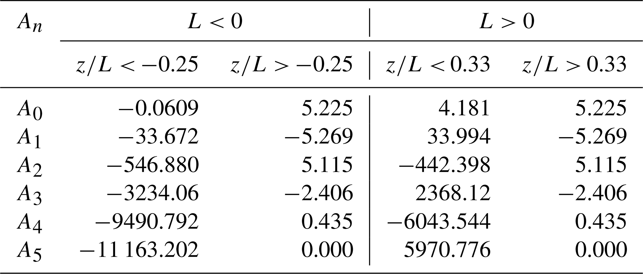
where L is the Monin–Obukhov length, and the values of A_n are given in Table 1, and also available in Alinot and Masson (2005).

Table 1 Coefficients of A_n for defining C_3ϵ from Alinot and Masson (2005).

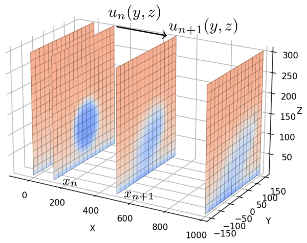
The structure of the parabolic Eqs. (1a)–(1g) allows for an efficient solution algorithm to be constructed that accurately captures the three-dimensional behavior of turbine wakes. Starting from a given inflow profile $u_{\mathrm{0}}(x_{\mathrm{0}},y,z)$ at an initial streamwise position x₀, the solution planes $u(x,y,z)$ for downstream locations can be determined through an implicit marching process (see Fig. 1). Details on the numerical solution algorithm are discussed below in Sect. 2.3.

Figure 1 Schematic showing the parabolized RANS solution process by marching planes of the velocity variable u(y,z) downstream through the domain.

Note that this RANS formulation eliminates the ability for flow information to travel in the upstream direction, as the parabolization process removes any elliptic behavior of the solution. This means that the effect of the turbine induction field is not included in these calculations, so any flow slowdown or acceleration due to blockage effects will be missing. However, superimposing the turbine induction field onto the RANS solution may be possible, as discussed in Sect. 6.

2.1.1 Pressure Poisson equation

In the parabolic formulation, enforcing continuity (Eq. 1a) is possible by developing the appropriate pressure Poisson equation. Taking the divergence of the momentum Eqs. (1b)–(1d) and applying the continuity Eq. (1a) leads to the following equation for pressure:

$$\begin{array}{}\text{(6)}& \begin{array}{rl}{\displaystyle \frac{\mathrm{1}}{\mathit{\rho }}}\left({\displaystyle \frac{{\partial }^{\mathrm{2}}p}{\partial y^{\mathrm{2}}}}+{\displaystyle \frac{{\partial }^{\mathrm{2}}p}{\partial z^{\mathrm{2}}}}\right)=& -{\displaystyle \frac{\partial u_j}{\partial x_i}}{\displaystyle \frac{\partial u_i}{\partial x_j}}+g\mathit{\beta }{\displaystyle \frac{\partial \mathrm{\Theta }}{\partial z}}\\ & +{\displaystyle \frac{\partial {\mathit{\nu }}_{\mathrm{T}}}{\partial x_i}}\left({\displaystyle \frac{{\partial }^{\mathrm{2}}{u}_i}{\partial y^{\mathrm{2}}}}+{\displaystyle \frac{{\partial }^{\mathrm{2}}{u}_i}{\partial z^{\mathrm{2}}}}\right)\\ & +{\displaystyle \frac{{\partial }^{\mathrm{2}}{\mathit{\nu }}_{\mathrm{T}}}{\partial y\partial x_i}}{\displaystyle \frac{\partial u_i}{\partial y}}+{\displaystyle \frac{{\partial }^{\mathrm{2}}{\mathit{\nu }}_{\mathrm{T}}}{\partial z\partial x_i}}{\displaystyle \frac{\partial u_i}{\partial z}}\\ =& S_{\mathrm{p}}.\end{array}\end{array}$$

Note that the second derivative of pressure, ${\partial }^{\mathrm{2}}p/\partial x^{\mathrm{2}}$, is neglected in the left-hand side of Eq. (6) as changes in the streamwise direction are assumed to be small relative to the y and z directions.

While many efficient algorithms exist to solve the two-dimensional Poisson problem, Eq. (6) can be reformulated as a parabolic diffusion problem if we assume that the pressure also depends on an artificial time τ variable such that

$$\begin{array}{}\text{(7)}& {\displaystyle \frac{\partial p}{\partial \mathit{\tau }}}=-\left({\displaystyle \frac{{\partial }^{\mathrm{2}}p}{\partial y^{\mathrm{2}}}}+{\displaystyle \frac{{\partial }^{\mathrm{2}}p}{\partial z^{\mathrm{2}}}}\right)+\mathit{\rho }{S}_{\mathrm{p}}.\end{array}$$

As the solution to Eq. (7) reaches a steady state, where $\partial p/\partial \mathit{\tau }\to \mathrm{0}$, we see that the pressure also satisfies the original Eq. (6). However, the same solution algorithm used to solve Eqs. (1b)–(1g) can also be applied to Eq. (7), which simplifies the overall implementation as described in Sect. 2.3.

2.2 Inflow and boundary conditions

Following Alinot and Masson (2005), the inflow conditions to the RANS model are based on Monin–Obukhov similarity theory for thermally stratified atmospheric surface layers over uniform flat terrain. Note that this RANS model is applicable to the near-surface layer close to the ground and cannot capture complex situations such as low-level jets, among other limitations (van der Laan et al., 2017). However, for the ABL profiles considered in the current study, this model sufficiently reproduces the inflow in the rotor disk regions for offshore wind turbines. When combined with the parabolic formulation in Eqs. (1a)–(1g), this leads to a consistent approach for handling the effects of stratification in both the wake and background inflow. In this formulation, the Monin–Obukhov length L is calculated as

$$\begin{array}{}\text{(8)}& L={\displaystyle \frac{u_{\ast }^{\mathrm{2}}{T}_{\mathrm{w}}}{\mathit{\kappa }g{T}_{\ast }}},\end{array}$$

where g is the gravitational constant, κ is the von Karman constant, T_w is the wall temperature, the friction velocity $u_{\ast }=\sqrt{{\mathit{\tau }}_{\mathrm{w}}/\mathit{\rho }}$ for a given wall shear stress τ_w, the temperature $T_{\ast }=-q_{\mathrm{w}}/\left(\mathit{\rho }{c}_p{u}_{\ast }\right)$, the surface heat flux is q_w, and the heat capacity is c_p. In all simulations considered here, κ = 0.42. The non-dimensional wind shear ϕ_m is expressed as

$$\begin{array}{}\text{(9)}& {\mathit{\varphi }}_{\mathrm{m}}\left({\displaystyle \frac{z}{L}}\right)=\left\{\begin{array}{ll}{\left(\mathrm{1}-\mathrm{16}{\displaystyle \frac{z}{L}}\right)}^{-\mathrm{1}/\mathrm{4}},& L<\mathrm{0}\\ \mathrm{1}+\mathrm{5}{\displaystyle \frac{z}{L}},& L\ge \mathrm{0}\end{array}\right..\end{array}$$

A similar non-dimensional profile ϕ_ϵ for the dissipation variable is also used:

$$\begin{array}{}\text{(10)}& {\mathit{\varphi }}_{\mathit{ϵ}}=\left\{\begin{array}{ll}\mathrm{1}-\frac{z}{L}& L<\mathrm{0}\\ {\mathit{\varphi }}_{\mathrm{m}}\left(\frac{z}{L}\right)-\frac{z}{L}& L\ge \mathrm{0}\end{array}\right..\end{array}$$

At the inlet of the domain, the horizontal velocity profile u_h is calculated using the Monin–Obukhov logarithmic profile:

$$\begin{array}{}\text{(11)}& \begin{array}{rl}& u_{\mathrm{h}}\left(z\right)\\ & =\left\{\begin{array}{ll}\frac{u_{\ast }}{\mathit{\kappa }}\left[\begin{array}{c}\ln (z/z_{\mathrm{0}})\\ +\ln \left(\frac{\mathrm{8}{\mathit{\varphi }}_{\mathrm{m}}^{\mathrm{4}}(z/L)}{\left({\mathit{\varphi }}_{\mathrm{m}}\right(z/L)+\mathrm{1}{)}^{\mathrm{2}}({\mathit{\varphi }}_{\mathrm{m}}^{\mathrm{2}}(z/L)+\mathrm{1})}\right)\\ -\frac{\mathit{\pi }}{\mathrm{2}}+\mathrm{2}\arctan \left(\frac{\mathrm{1}}{{\mathit{\varphi }}_{\mathrm{m}}(z/L)}\right)\end{array}\right],& L<\mathrm{0},\\ \frac{u_{\ast }}{\mathit{\kappa }}\left[\ln (z/z_{\mathrm{0}})+{\mathit{\varphi }}_{\mathrm{m}}(z/L)-\mathrm{1}\right],& L\ge \mathrm{0},\end{array}\right.\end{array}\end{array}$$

where z₀ is the value of the surface roughness at the lower boundary. The horizontal velocity $u_{\mathrm{h}}=\sqrt{u_{\mathrm{0}}^{\mathrm{2}}+v_{\mathrm{0}}^{\mathrm{2}}}$ is further decomposed into streamwise u₀ and lateral v₀ velocity components so that the wind direction matches the desired θ(z) veer profile. Note that the veer profile θ(z) is not given by the Monin–Obukhov similarity theory and must be determined from alternate sources, such as LES precursor profiles or from measured inflow profiles. By convention, we also configure the wind direction profile so that the velocity at hub height (z=z_h) is purely in the streamwise direction.

A similar modified logarithmic profile is used for the initial temperature profile:

$$\begin{array}{}\text{(12)}& \begin{array}{rl}& {\mathrm{\Theta }}_{\mathrm{0}}\left(z\right)-T_{\mathrm{w}}\\ & =\left\{\begin{array}{ll}\frac{T_{\ast }}{\mathit{\kappa }}\left[\begin{array}{c}\ln (z/z_{\mathrm{0}})\\ -\mathrm{2}\ln \left[\frac{\mathrm{1}}{\mathrm{2}}\left(\mathrm{1}+{\mathit{\varphi }}_{\mathrm{m}}^{-\mathrm{2}}(z/L)\right)\right]\end{array}\right],& L<\mathrm{0}\\ \frac{T_{\ast }}{\mathit{\kappa }}\left[\ln (z/z_{\mathrm{0}})+{\mathit{\varphi }}_{\mathrm{m}}(z/L)-\mathrm{1}\right],& L\ge \mathrm{0}\end{array}\right..\end{array}\end{array}$$

The initial kinetic energy and dissipation profiles matched those used in Alinot and Masson (2005):

$$\begin{array}{}\text{(13)}& {\displaystyle }{k}_{\mathrm{0}}\left(z\right)& {\displaystyle }=\mathrm{5.48}{C}_{\mathrm{k}}{u}_{\ast }^{\mathrm{2}}\sqrt{{\displaystyle \frac{{\mathit{\varphi }}_{\mathit{ϵ}}(z/L)}{{\mathit{\varphi }}_{\mathrm{m}}(z/L)}}},\text{(14)}& {\displaystyle }{\mathit{ϵ}}_{\mathrm{0}}\left(z\right)& {\displaystyle }={\displaystyle \frac{u_{\ast }^{\mathrm{3}}}{\mathit{\kappa }z}}{\mathit{\varphi }}_{\mathit{ϵ}}(z/L),\end{array}$$

where C_k is an adjustable parameter used to adjust the ambient RANS turbulent kinetic energy k to be roughly similar to the corresponding LES k at the turbine hub height. Note that the use of the C_k applies only to the inflow profile, not to the boundary conditions or the interior of the RANS domain, and is not used in the work of Alinot and Masson (2005) or other elliptic RANS models.

At the lower boundary $z=z_{min}$, the following Dirichlet boundary conditions are imposed:

$$\begin{array}{}\text{(15)}& \begin{array}{rl}& u=u_{\mathrm{0}}\left(z_{min}\right),v=v_{\mathrm{0}}\left(z_{min}\right),w\left(z_{min}\right)=\mathrm{0},\\ & \mathrm{\Theta }={\mathrm{\Theta }}_{\mathrm{0}}\left(z_{min}\right),k\left(z_{min}\right)=\mathrm{5.48}{u}_{\ast }^{\mathrm{2}}\sqrt{{\displaystyle \frac{{\mathit{\varphi }}_{\mathit{ϵ}}(z/L)}{{\mathit{\varphi }}_{\mathrm{m}}(z/L)}}},\\ & \mathit{ϵ}={\mathit{ϵ}}_{\mathrm{0}}\left(z_{min}\right),p=\mathrm{0}.\end{array}\end{array}$$

At the upper boundary $z=z_{max}$, a combination of Dirichlet and Neumann boundary conditions is used:

$$\begin{array}{}\text{(16)}& \begin{array}{rl}& u=u_{\mathrm{0}}\left(z_{max}\right),v=v_{\mathrm{0}}\left(z_{max}\right),{\displaystyle \frac{\partial w}{\partial z}}=\mathrm{0},{\displaystyle \frac{\partial \mathrm{\Theta }}{\partial z}}=\mathrm{\Gamma },\\ & k\left(z_{max}\right)=\mathrm{5.48}{u}_{\ast }^{\mathrm{2}}\sqrt{{\displaystyle \frac{{\mathit{\varphi }}_{\mathit{ϵ}}(z/L)}{{\mathit{\varphi }}_{\mathrm{m}}(z/L)}}},{\displaystyle \frac{\partial \mathit{ϵ}}{\partial z}}=\mathrm{0},\\ & {\displaystyle \frac{\partial p}{\partial z}}=\mathrm{0},\end{array}\end{array}$$

where Γ is the specified lapse rate. At the lateral boundaries $y=y_{min},y_{max}$, the following boundary conditions are applied:

$$\begin{array}{}\text{(17)}& \begin{array}{rl}& u\left(z\right)=u_{\mathrm{0}}\left(z\right),v\left(z\right)=v_{\mathrm{0}}\left(z\right),w\left(z\right)=\mathrm{0},\mathrm{\Theta }\left(z\right)={\mathrm{\Theta }}_{\mathrm{0}}\left(z\right),\\ & {\displaystyle \frac{\partial k}{\partial y}}=\mathrm{0},{\displaystyle \frac{\partial \mathit{ϵ}}{\partial y}}=\mathrm{0},{\displaystyle \frac{\partial p}{\partial y}}=\mathrm{0}.\end{array}\end{array}$$

2.3 Numerical solution

The numerical solution to Eqs. (1a)–(1g) is computed using an iterative alternating-direction implicit (ADI) approach. This allows for an efficient and robust marching procedure by splitting the y and z differentiations into separate stages which can be quickly calculated using a tri-diagonal matrix solver. The implicit nature of the algorithm also allows for relatively large Δx steps in the streamwise direction. Using the notation $u(x,y,z)=U_{ij}^n$ to indicate the discretized flow variables at the location $(x_n,y_i,z_j)$, the following second-order differentiation stencils for the first and second derivatives in the y and z directions can be written as

$$\begin{array}{}\text{(18a)}& {\displaystyle }\begin{array}{rl}& D_y{U}_{ij}={\displaystyle \frac{U_{i+\mathrm{1},j}-U_{i-\mathrm{1},j}}{\mathrm{2}}},\\ & D_y^{\mathrm{2}}{U}_{ij}=U_{i+\mathrm{1},j}-\mathrm{2}{U}_{i,j}+U_{i-\mathrm{1},j}\end{array}\text{(18b)}& {\displaystyle }\begin{array}{rl}& D_z{U}_{ij}={\displaystyle \frac{U_{i,j+\mathrm{1}}-U_{i,j-\mathrm{1}}}{\mathrm{2}}},\\ & D_z^{\mathrm{2}}{U}_{ij}=U_{i,j+\mathrm{1}}-\mathrm{2}{U}_{i,j}+U_{i,j-\mathrm{1}}.\end{array}\end{array}$$

In the advection terms of Eqs. (1a)–(1g), the averaged values of the velocities and turbulent viscosity between position x_n and x_n+1 are used:

$$\begin{array}{rl}& {\stackrel{\mathrm{̃}}{U}}_{ij}={\displaystyle \frac{U_{ij}^{n+\mathrm{1}}+U_{ij}^n}{\mathrm{2}}},{\stackrel{\mathrm{̃}}{V}}_{ij}={\displaystyle \frac{V_{ij}^{n+\mathrm{1}}+V_{ij}^n}{\mathrm{2}}},\\ & {\stackrel{\mathrm{̃}}{W}}_{ij}={\displaystyle \frac{W_{ij}^{n+\mathrm{1}}+W_{ij}^n}{\mathrm{2}}},{\stackrel{\mathrm{̃}}{\mathit{\nu }}}_{\mathrm{T},ij}={\displaystyle \frac{{\mathit{\nu }}_{\mathrm{T},ij}^{n+\mathrm{1}}+{\mathit{\nu }}_{\mathrm{T},ij}^n}{\mathrm{2}}}.\end{array}$$

Solving each of the Eqs. (1b)–(1g) and (7) uses a two-stage process, where advancing from x_n to x_n+1 requires two half-steps each $\mathrm{\Delta }x/\mathrm{2}$ in size. Taking the solution of the x momentum Eq. (1b) as an example, the first half-step solves for $U_{ij}^{n+\mathrm{1}/\mathrm{2}}$ given $U_{ij}^n$ by treating the y direction implicitly and the z direction explicitly:

$$\begin{array}{}\text{(19a)}& \begin{array}{rl}& \left[{\displaystyle \frac{{\stackrel{\mathrm{̃}}{U}}_{ij}}{\mathrm{\Delta }x/\mathrm{2}}}+\left({\stackrel{\mathrm{̃}}{V}}_{ij}-{\displaystyle \frac{D_y{\stackrel{\mathrm{̃}}{\mathit{\nu }}}_{\mathrm{T}}}{\mathrm{\Delta }y}}\right){\displaystyle \frac{D_y}{\mathrm{\Delta }y}}-(\mathit{\nu }+{\stackrel{\mathrm{̃}}{\mathit{\nu }}}_{\mathrm{T}}){\displaystyle \frac{D_y^{\mathrm{2}}}{(\mathrm{\Delta }y{)}^{\mathrm{2}}}}\right]U_{ij}^{n+\mathrm{1}/\mathrm{2}}\\ =& \left[{\displaystyle \frac{\stackrel{\mathrm{̃}}{U_{ij}}}{\mathrm{\Delta }x/\mathrm{2}}}-\left({\stackrel{\mathrm{̃}}{W}}_{ij}-{\displaystyle \frac{D_z{\stackrel{\mathrm{̃}}{\mathit{\nu }}}_{\mathrm{T}}}{\mathrm{\Delta }z}}\right){\displaystyle \frac{D_z}{\mathrm{\Delta }z}}+(\mathit{\nu }+{\stackrel{\mathrm{̃}}{\mathit{\nu }}}_{\mathrm{T}}){\displaystyle \frac{D_z^{\mathrm{2}}}{(\mathrm{\Delta }z{)}^{\mathrm{2}}}}\right]U_{ij}^n\\ & +f_x^n-{\displaystyle \frac{p_{ij}^{n+\mathrm{1}}-p_{ij}^n}{\mathit{\rho }\mathrm{\Delta }x}}.\end{array}\end{array}$$

The second half-step then advances the solution from $U_{ij}^{n+\mathrm{1}/\mathrm{2}}$ to $U_{ij}^n$ by treating the z direction implicitly and the y direction explicitly:

$$\begin{array}{}\text{(19b)}& \begin{array}{rl}& \left[{\displaystyle \frac{{\stackrel{\mathrm{̃}}{U}}_{ij}}{\mathrm{\Delta }x/\mathrm{2}}}+\left({\stackrel{\mathrm{̃}}{W}}_{ij}-{\displaystyle \frac{D_z{\stackrel{\mathrm{̃}}{\mathit{\nu }}}_{\mathrm{T}}}{\mathrm{\Delta }z}}\right){\displaystyle \frac{D_z}{\mathrm{\Delta }z}}-(\mathit{\nu }+{\stackrel{\mathrm{̃}}{\mathit{\nu }}}_{\mathrm{T}}){\displaystyle \frac{D_z^{\mathrm{2}}}{(\mathrm{\Delta }z{)}^{\mathrm{2}}}}\right]U_{ij}^{n+\mathrm{1}}\\ =& \left[{\displaystyle \frac{{\stackrel{\mathrm{̃}}{U}}_{ij}}{\mathrm{\Delta }x/\mathrm{2}}}-\left({\stackrel{\mathrm{̃}}{V}}_{ij}-{\displaystyle \frac{D_y{\stackrel{\mathrm{̃}}{\mathit{\nu }}}_{\mathrm{T}}}{\mathrm{\Delta }y}}\right){\displaystyle \frac{D_y}{\mathrm{\Delta }y}}+(\mathit{\nu }+{\stackrel{\mathrm{̃}}{\mathit{\nu }}}_{\mathrm{T}}){\displaystyle \frac{D_y^{\mathrm{2}}}{(\mathrm{\Delta }y{)}^{\mathrm{2}}}}\right]U_{ij}^{n+\mathrm{1}/\mathrm{2}}\\ & +f_x^{n+\mathrm{1}/\mathrm{2}}-{\displaystyle \frac{p_{ij}^{n+\mathrm{1}}-p_{ij}^n}{\mathit{\rho }\mathrm{\Delta }x}}.\end{array}\end{array}$$

Equations (19a) and (19b) can be efficiently solved using a tri-diagonal matrix solver due to the banded nature of the differentiation stencils. Similar two-step, discretized equations can be written for Eqs. (1c)–(1g) and (7), noting that for the pressure solution, the steps in Δx are replaced with steps in Δτ.

To calculate a consistent solution for all flow variables, an iterative approach is used at every downstream position. As outlined in Algorithm 1, starting from a known solution at x_n each of the governing equations is solved in sequence for the next values of Uⁿ⁺¹, Vⁿ⁺¹, Wⁿ⁺¹, kⁿ⁺¹, ϵⁿ⁺¹, Θⁿ⁺¹, and pⁿ⁺¹. These solutions are repeated until the difference between successive iterations converge below a predefined tolerance.

Algorithm 1 To advance the RANS solution to x_n+1 from x_n.

Set iteration counter m=0

Set ${\mathit{\psi }}_{ij}^{n+\mathrm{1},m}$ = ${\mathit{\psi }}_{ij}^n$ for $\mathit{\psi }=U,V,W,k,\mathit{ϵ},\mathrm{\Theta },p$

while $|{\mathit{\psi }}_{ij}^{n+\mathrm{1},m}-{\mathit{\psi }}_{ij}^{n+\mathrm{1},m-\mathrm{1}}|>{\mathit{\epsilon }}_{TOL}$ do

m=m+1

Calculate $U_{ij}^{n+\mathrm{1},m}$ from $U_{ij}^n$ using Eq. (19)

Calculate $V_{ij}^{n+\mathrm{1},m}$ from $V_{ij}^n$

Calculate $W_{ij}^{n+\mathrm{1},m}$ from $W_{ij}^n$

Calculate $k_{ij}^{n+\mathrm{1},m}$ from $k_{ij}^n$

Calculate ${\mathit{ϵ}}_{ij}^{n+\mathrm{1},m}$ from ${\mathit{ϵ}}_{ij}^n$

Calculate ${\mathrm{\Theta }}_{ij}^{n+\mathrm{1},m}$ from ${\mathrm{\Theta }}_{ij}^n$

Calculate $p_{ij}^{n+\mathrm{1},m}$ from $p_{ij}^n$

end while

The simulations presented below typically used grid sizes of $(N_y,N_z)=(\mathrm{81},\mathrm{41})$ with mesh sizes of Δy×Δz = 10 m × 10 m for the IEA 15 MW reference turbine. Initial refinement studies indicated that streamwise step sizes of $\mathrm{\Delta }x/R$ = 0.5–1 were possible using this formulation, where R = 120 m is the turbine radius of the IEA 15 MW, and provided a good balance between accuracy and computational efficiency. For the single-turbine runs discussed in Sect. 4, the simulations required between 10–25 s on one Intel Xeon Platinum 8480+ CPU.

2.4 Actuator disk turbine model

The parabolic formulation of the RANS momentum Eqs. (1b)–(1d) provides a natural means to represent the wind turbine in the computational domain. Similar to other high-fidelity wind turbine simulation codes (see Sect. 3.1), the turbine rotor forces can be included as body forces in the momentum equations through an actuator disk model. Multiple choices of actuator disk models are available in the literature, but the initial comparisons shown in Sect. 4.1–4.4 use the uniformly loaded actuator disk model due to its simplicity. In Sect. 4.5, comparisons of the turbine wake using the Joukowski actuator disk model (Sørensen et al., 2020) are shown and are able to capture additional effects, including veer–swirl interactions and more realistic near-wake profiles.

The initial uniformly loaded disk model computes the rotor disk forces based on the density ρ, thrust coefficient C_t, upstream velocity U_up, and rotor normal ${\widehat{\mathit{n}}}_{\mathrm{T}}$:

$$\begin{array}{}\text{(20)}& {\mathit{f}}_{\mathrm{T}}={\displaystyle \frac{\mathrm{1}}{\mathrm{2}}}{C}_{\mathrm{t}}\mathit{\rho }{U}_{\text{up}}^{\mathrm{2}}g\left(r\right){\widehat{\mathit{n}}}_{\mathrm{T}}.\end{array}$$

The thrust coefficient is given as a predetermined function of the free-stream wind speed C_t=C_t(U_up), and U_up is computed using the rotor-averaged velocity from the solution immediately upstream of the turbine location. In Eq. (20) the actuator force f_T is applied to all points on the rotor disk with the hub location $(x,y,z)=(x_{\mathrm{T}},y_{\mathrm{T}},z_{\mathrm{h}})$. A blending function g(r), where $r=\sqrt{(y-y_{\mathrm{T}}{)}^{\mathrm{2}}+(z-z_{\mathrm{h}}{)}^{\mathrm{2}}}$, is used to avoid a sharp discontinuity in the applied force at the rotor disk edge. In the current work, the hyperbolic tangent blending function

$$\begin{array}{}\text{(21)}& g\left(r\right)={\displaystyle \frac{\mathrm{1}}{\mathrm{2}}}\left[\mathrm{1}-\tanh \left({\displaystyle \frac{r-R}{r_{\mathrm{\Delta }}}}\right)\right]\end{array}$$

is used, where r_Δ is a smoothing parameter. Note that the actuator force f_T is calculated as a force per unit area and is divided by Δx to be included as a body force per unit volume in Eqs. (1b)–(1d). Multiple turbines and wake steering effects can be captured by superposing multiple actuator turbine forces and adjusting the directions of the rotor normals.

2.5 Calibration of the RANS model

The RANS closure model was calibrated by comparing the rotor plane velocity U in the RANS against corresponding planes from LES for the cases listed in Table 3 to be described in more detail later. Similar to the approach in Cheung et al. (2025), the calibration only compares the rotor planes at a distance of 4D and 6D downstream of the turbine since the RANS model does not account for the hub and nacelle regions present in the LES. These downstream distances were also chosen based on the typical streamwise spacings and regions of interest for offshore wind farms, but the calibration process can be repeated using other downstream distances in future studies. The cost function for the calibration is the ℒ₂ norm of the difference in the streamwise velocity between the LES and the RANS rotor planes. The extent of the rotor plane for the calibration is $y\in [-\mathrm{1.5}D,\mathrm{1.5}D]$ from the center of the turbine disk and $z\in [\mathrm{0},\mathrm{400}\mathrm{m}]$, discretized into a grid of uniformly spaced [50,21] points. The parameters for calibration were picked to be the coefficients, C_μ, C_1ε, C_2ε, of the k−ϵ RANS closure model and the coefficient C_k for the inflow boundary conditions in Eq. (13). The L-BFGS-B (Byrd et al., 1995; Zhu et al., 1997) algorithm as implemented in SciPy was used for the calibration. The optimal values from this calibration were C_μ=0.076, C_1ε=1.46, C_2ε=1.92, and C_k=0.72 for the case with medium wind speed (WS) and C_k=0.40 for the low-WS case. Comparisons of calibrated RANS results in Figs. 4, 5, and 7 show qualitative agreement between the wake velocity planes from the calibration cases, especially at x=4D and x=6D. As further validation, Fig. 6 shows great qualitative agreement between turbulent kinetic energy (TKE) in the RANS and the LES calculations, noting that TKE was not used as part of the calibration calculations. These results are further discussed in Sect. 4.

Table 2 Input parameters for the low- and high-WS stable-atmosphere cases.

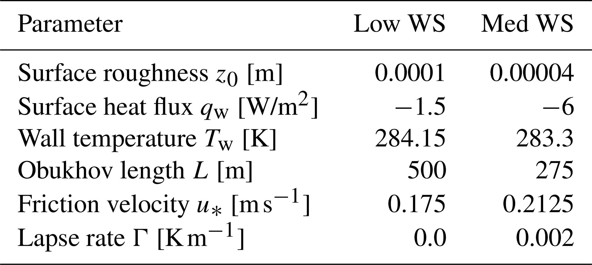
Table 3 Hub-height wind speed conditions used in the turbine wake study. All values are taken from the simulated atmospheric boundary layer as described in Sect. 3.3. Note that the calculation of TI in the table is based on the standard deviation of the horizontal velocity, non-dimensionalized by the mean of the horizontal velocity.

3 Simulation comparison details

In the following sections, we provide details on the high-fidelity LES methodology used for calibration and comparisons of the RANS models. The equivalent semi-empirical FLORIS wake models are also discussed, and information on the atmospheric conditions and turbine configuration used in this study is included in Sect. 3.3.

3.1 Kynema-SGF code description

Following an approach similar to that described in Cheung et al. (2025), LES data were collected for calibration and comparison purposes by performing simulations with Kynema-SGF (formerly AMR-Wind) (Sharma et al., 2024; Sprague et al., 2020; Kuhn et al., 2025), a massively parallel, block-structured adaptive-mesh solver designed for simulating wind turbines and wind farms. Kynema-SGF solves the incompressible and low-Mach-number formulations of the Navier–Stokes equations with transport equations for temperature, subgrid-scale kinetic energy, and additional scalars required for wind farm LES. The spatial discretization employs a second-order finite-volume method, coupled with a second-order temporal-integration scheme. Kynema-SGF includes comprehensive atmospheric boundary layer (ABL) physics modules: ABL forcing, Boussinesq buoyancy, Coriolis effects, and body forcing to preserve precursor-derived inflow conditions under turbine blockage. It also includes forcing terms from an actuator line turbine representation (following implementations in Brown et al., 2025, and Hsieh et al., 2025) that is derived from coupling to OpenFAST (Jonkman et al., 2018; NREL, 2023; Brown et al., 2024). The framework leverages AMReX for data structures, parallelism abstractions, and performance portability across heterogeneous computing architectures (Zhang et al., 2019), demonstrating robust performance across diverse systems and applications (Fedeli et al., 2022; Henry de Frahan et al., 2022, 2024).

3.2 FLORIS model description

The RANS model is compared to a steady-state engineering model using the FLOw Redirection and Induction in Steady-state (FLORIS) tool (NREL, 2025). FLORIS is a widely used wind farm simulation software designed for wind farm layout and control optimization that can predict the time-averaged three-dimensional flow field and turbine power of a wind farm. Following Yalla et al. (2025), the empirical Gaussian model in FLORIS is used here to represent the steady-state wakes. In this model, the normalized wake velocity deficit, $u/U_{\mathrm{\infty }}$, is represented by a Gaussian centered on lateral and vertical wake centers, δ_y and δ_z, as

$$\begin{array}{}\text{(22)}& u/U_{\mathrm{\infty }}\left(x\right)=\mathrm{1}-C\exp \left(-{\displaystyle \frac{(y-{\mathit{\delta }}_y(x){)}^{\mathrm{2}}}{\mathrm{2}{\mathit{\sigma }}_y(x{)}^{\mathrm{2}}}}-{\displaystyle \frac{(z-{\mathit{\delta }}_z(x){)}^{\mathrm{2}}}{\mathrm{2}{\mathit{\sigma }}_z(x{)}^{\mathrm{2}}}}\right).\end{array}$$

The standard deviations, σ_y,z(x), represent the wake widths as a function of streamwise distance, x, and are modeled as

$$\begin{array}{}\text{(23)}& {\mathit{\sigma }}_{y,z}\left(x\right)=\underset{\mathrm{0}}{\overset{x}{\int }}\sum _{i=\mathrm{0}}^n{k}_i{\mathbf{1}}_{[b_i,b_{i+\mathrm{1}}]}\left(x^{\prime }\right)\mathrm{d}{x}^{\prime }+M_j\left(x\right)\mathrm{d}{x}^{\prime }+{\mathit{\sigma }}_{y_{\mathrm{0}},z_{\mathrm{0}}},\end{array}$$

which depends on several adjustable parameters, including a constant initial wake width, ${\mathit{\sigma }}_{y_{\mathrm{0}},z_{\mathrm{0}}}$, and a set of parameters, k_i, that control the wake expansion rate between break-point locations b_i and b_i+1. For each turbine (indexed by j), the wake widths also include a mixing term, M_j, that represents the effects of atmospheric turbulence intensity (TI) and wake overlap on wake spreading as

$$\begin{array}{}\text{(24)}& {\displaystyle }{M}_j\left(x\right){\displaystyle }={\mathit{\omega }}_{\mathrm{v}}\sqrt{\left[\sum _{\begin{array}{c}i=\mathrm{1}\\ i\ne j\end{array}}^{N_{turb}}{\left({\displaystyle \frac{{\mathrm{\Omega }}_{ij}{a}_i}{\left(\right(x_j-x_i)/D_i{)}^{\mathrm{2}}}}\right)}^{\mathrm{2}}+(\mathit{\gamma }I{)}^{\mathrm{2}}\right]},\end{array}$$

where Ω_ij quantifies the area of overlap of the wake of turbine i onto turbine j, a_i is the axial induction factor of the ith turbine, and I is the turbulence intensity. The parameters ω_v and γ can be adjusted to control the strength of the wake mixing term.

In Yalla et al. (2025), the empirical Gaussian model in FLORIS was calibrated using LES data from a 3×3 array of IEA 15 MW turbines operating in one of the stable-wind-condition scenarios considered in this study, specifically the med-WS case described in Sect. 3.3. Therefore, the calibrated empirical Gaussian parameters from Yalla et al. (2025) are directly applied here to compare FLORIS with the LES and RANS models. It is important to note that Yalla et al. (2025) focused on estimating annual energy production (AEP) for different wind farm flow control strategies and therefore calibrated the empirical Gaussian parameters based on turbine power rather than wake quantities of interest, which are the focus here.

3.3 Simulation cases

The comparisons between the RANS model, high-fidelity LES, and FLORIS calculations were done using two scenarios under stably stratified atmospheric conditions. These conditions were previously studied by Frederik et al. (2025), Brown et al. (2025), and Cheung et al. (2025) and contain the necessary shear, veer, and stratification effects for evaluating the accuracy of the parabolic RANS model. As described in Brown et al. (2025), the offshore ABL conditions are derived from floating-buoy lidar measurements taken near the coast of the New York Bight. Two scenarios representative of low-TI, stable conditions with wind speeds below rated were selected for this study (Tables 2 and 3). In Kynema-SGF, the precursor ABL simulations were generated by imposing negative surface ground temperature rates and adjusting the surface roughness z₀ until the horizontally averaged ABL profiles matched the desired targets. Similarly, the surface heat flux q_w and the surface roughness z₀ were adjusted under RANS inflow conditions to match the measured lidar profiles.

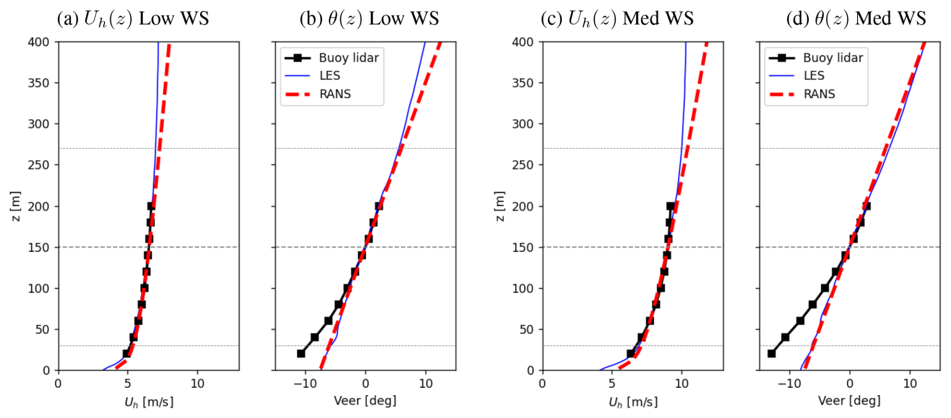
Figure 2 Inflow comparison between the RANS model, Kynema-SGF LES, and the floating-buoy lidar data for the horizontal wind speed U_h(z) and veer θ(z) profiles for the two ABL scenarios in Table 3.

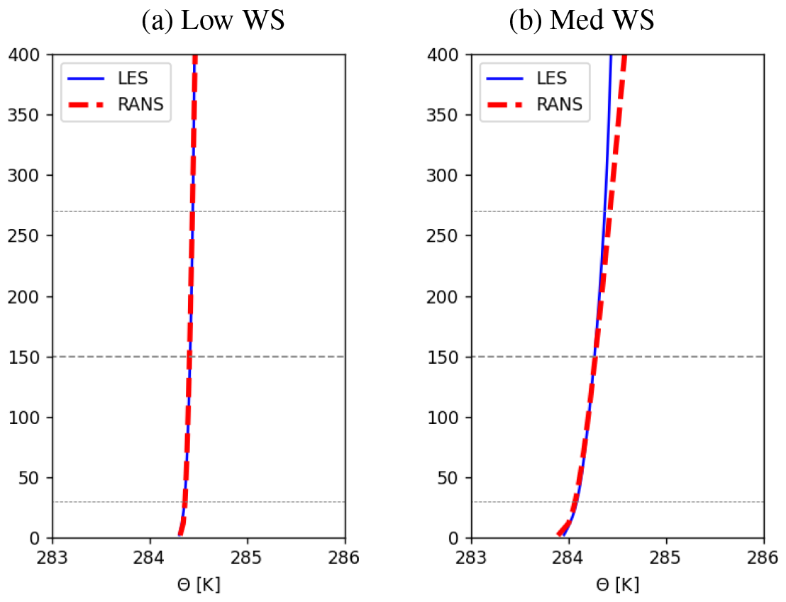
Figure 3 The comparison of the inflow temperature Θ(z) profiles between RANS and the Kynema-SGF LES computations.

A comparison of the Kynema-SGF LES, RANS, and buoy lidar profiles is shown in Figs. 2 and 3. For both the low-WS and med-WS cases, close agreement is observed between the Kynema-SGF and RANS horizontal velocity U_h profiles, as well as with the lidar measurements. Figure 2 also shows that the linear veer profile θ(z) used in the RANS inflow also matches the Kynema-SGF LES veer profile over the rotor disk.

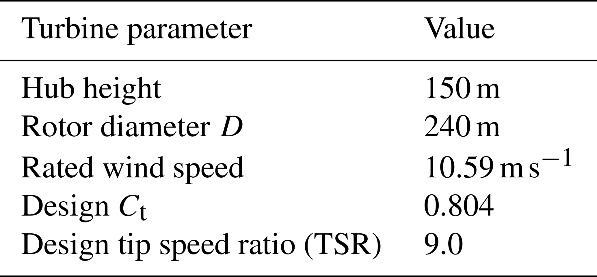
The offshore IEA 15 MW reference turbine is used for all wake comparisons in this study. The major characteristics of the IEA 15 MW turbine are given in Table 4, with additional details provided by Gaertner et al. (2020). In the Kynema-SGF LES simulations, the OpenFAST actuator line representation of the IEA 15 MW turbine is used with the open-source ROSCO (NREL, 2021) wind turbine controller. For the parabolic RANS and FLORIS model, the variation in the thrust coefficient C_t with wind speed is specified to match the operating curve of the IEA 15 MW design. In the single-turbine RANS calculations, the lateral and vertical extents were 800 m × 400 m.

Table 4 Details of the IEA 15 MW reference turbine.

4 Wind turbine wake comparisons

Comparisons of wake behavior between the SANDWake3D RANS model, Kynema-SGF LES, and FLORIS calculations are discussed in the following sections. The results for a single-turbine wake under low-WS and med-WS ABL conditions are considered first in Sect. 4.1, before examining the two-turbine case in Sect. 4.3. Lastly, the RANS model is demonstrated on a nine-turbine wind farm configuration in Sect. 4.4.

Note that in the following discussions regarding turbulence, the comparison of the turbulent kinetic energy k in RANS with the same quantity in the LES is limited by the fundamental assumptions used within the simulations themselves. The turbulence in the RANS calculations is determined by the closure model used in the k−ϵ formulation and assumed to be isotropic, while the majority of the turbulence is directly calculated in the LES and is shown to be anisotropic for stratified flows. Thus, a direct comparison of the two quantities should be interpreted from a qualitative standpoint, and quantitative differences may appear due to the nature of the calculations.

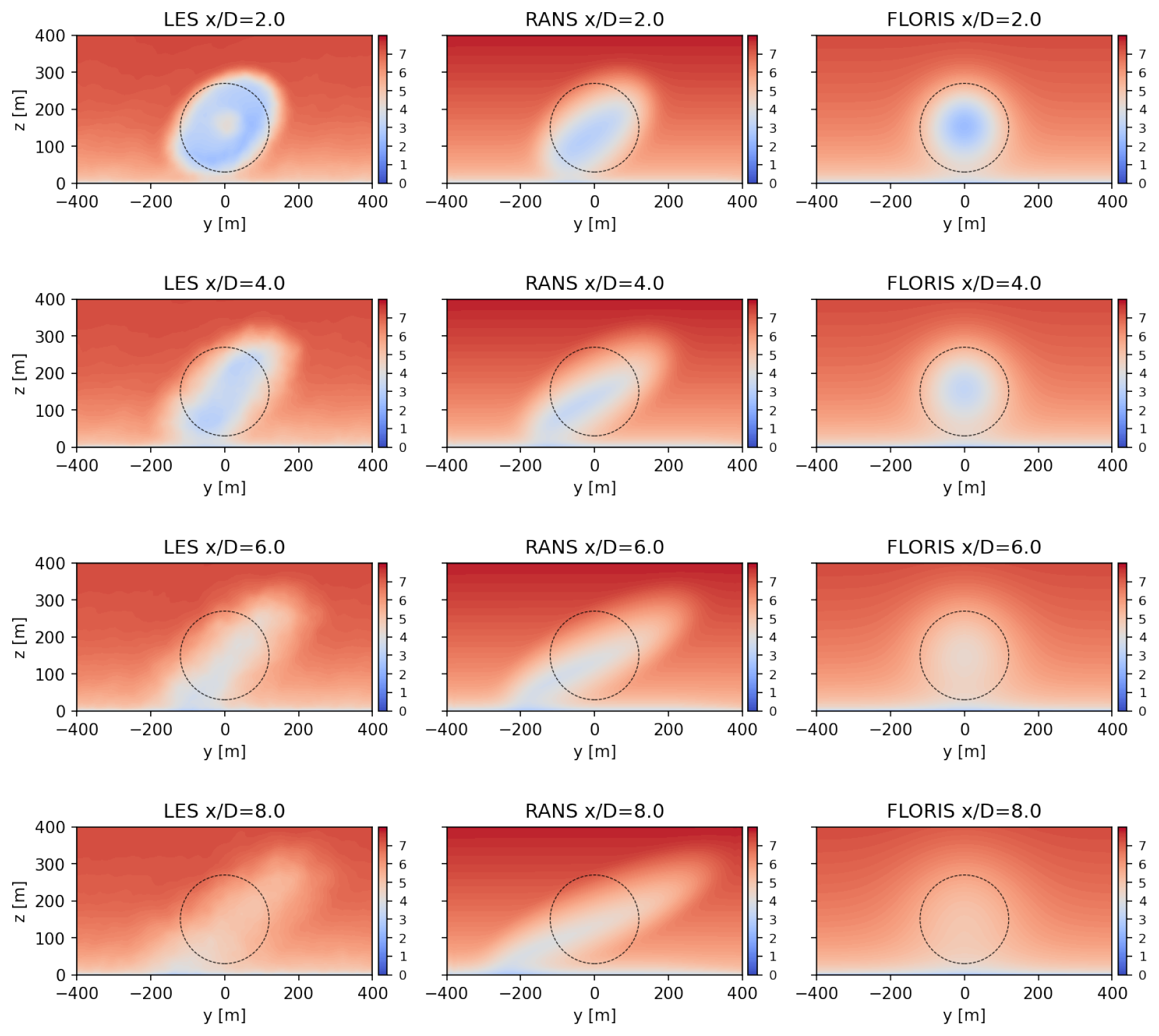
Figure 4 Comparison of the streamwise velocity u(y,z) for low-WS inflow conditions, as computed by the Kynema-SGF LES, SANDWake3D RANS, and FLORIS empirical Gaussian methods. Contours of u(y,z) are plotted with units of m s⁻¹ at distances $x/D=\mathrm{2}$, 4, 6, and 8 downstream of the turbine. The dashed circle corresponds to the location of the rotor disk of the IEA 15 MW reference turbine.

4.1 Single-turbine cases

A qualitative view of the wake evolution for the single-turbine configuration under low-WS ABL conditions is provided in Fig. 4. In this figure, the steady streamwise velocities for the LES, RANS, and FLORIS models are displayed at various rotor planes at different downstream distances ranging from x=2D to x=8D. From these plots, several observations can be made regarding the choice of wake model on the predicted wake behavior. When comparing the LES solutions against the RANS in the far wake, for x>5D, we see a similar degree of wake skew and stretching due to the ambient veer in the ABL. In the near-wake region, some differences in the centerline wake deficit can be seen, and this can be attributed to the difference between the uniformly loaded disk model in RANS and the actuator line model in Kynema-SGF. The latter model includes a nacelle and hub drag model and also captures the variation in loading near the blade root sections. This leads to lower centerline wake deficits compared to the RANS model immediately downstream of the rotor at x=2D, although this difference is less apparent by x=4D.

Compared to the LES and RANS results, the FLORIS empirical Gaussian model also generally captures the wake spread and deficit behavior for the single-turbine configuration and also accounts for the ambient shear from the inflow. However, the effects of veer are not directly included in the empirical Gaussian model, which instead reduces the overall wake deficit to account for the effects of veer on the power of downstream turbines. Wake skewing and stretching are also not present in the FLORIS wake results, which remain axisymmetric at all downstream locations by design.

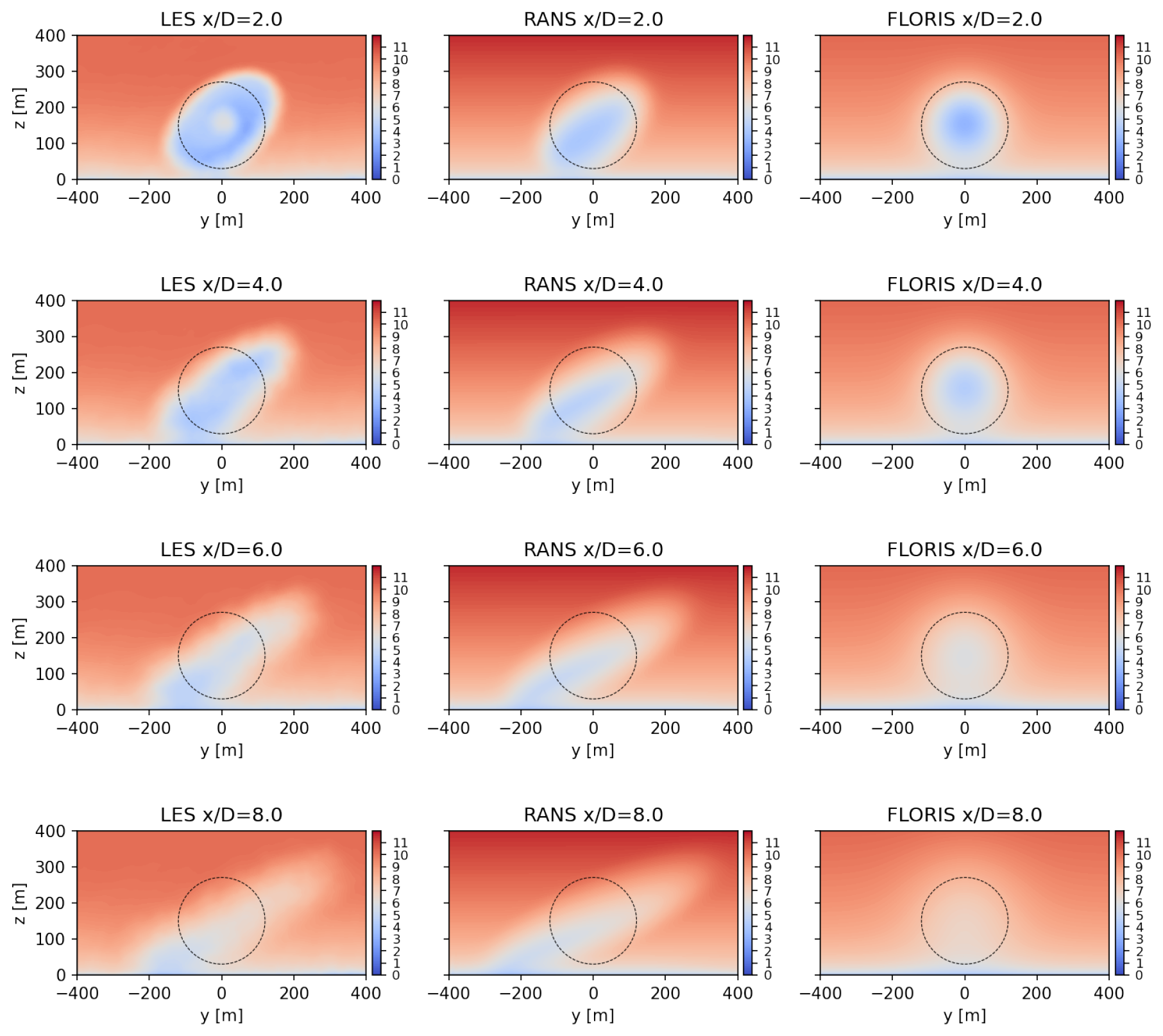
Figure 5 Comparison of the streamwise velocity u(y,z) for med-WS inflow conditions, as computed by the Kynema-SGF LES, SANDWake3D RANS, and FLORIS empirical Gaussian methods. Contours of u(y,z) are plotted with units of m s⁻¹ at distances $x/D=\mathrm{2}$, 4, 6, and 8 downstream of the turbine. The dashed circle corresponds to the location of the rotor disk of the IEA 15 MW reference turbine.

A similar comparison of the turbine wake behavior for med-WS conditions is shown in Fig. 5, and similar conclusions can be drawn between the LES, RANS, and FLORIS models. Both Kynema-SGF and SANDWake3D capture the effects of wake skewing and wake stretching, as opposed to the empirical Gaussian model. In the med-WS scenario, we also observe a unique impact of veer on the wake development in the LES and RANS results, where the wake deficits persist much farther downstream at lower elevations compared to higher elevations.

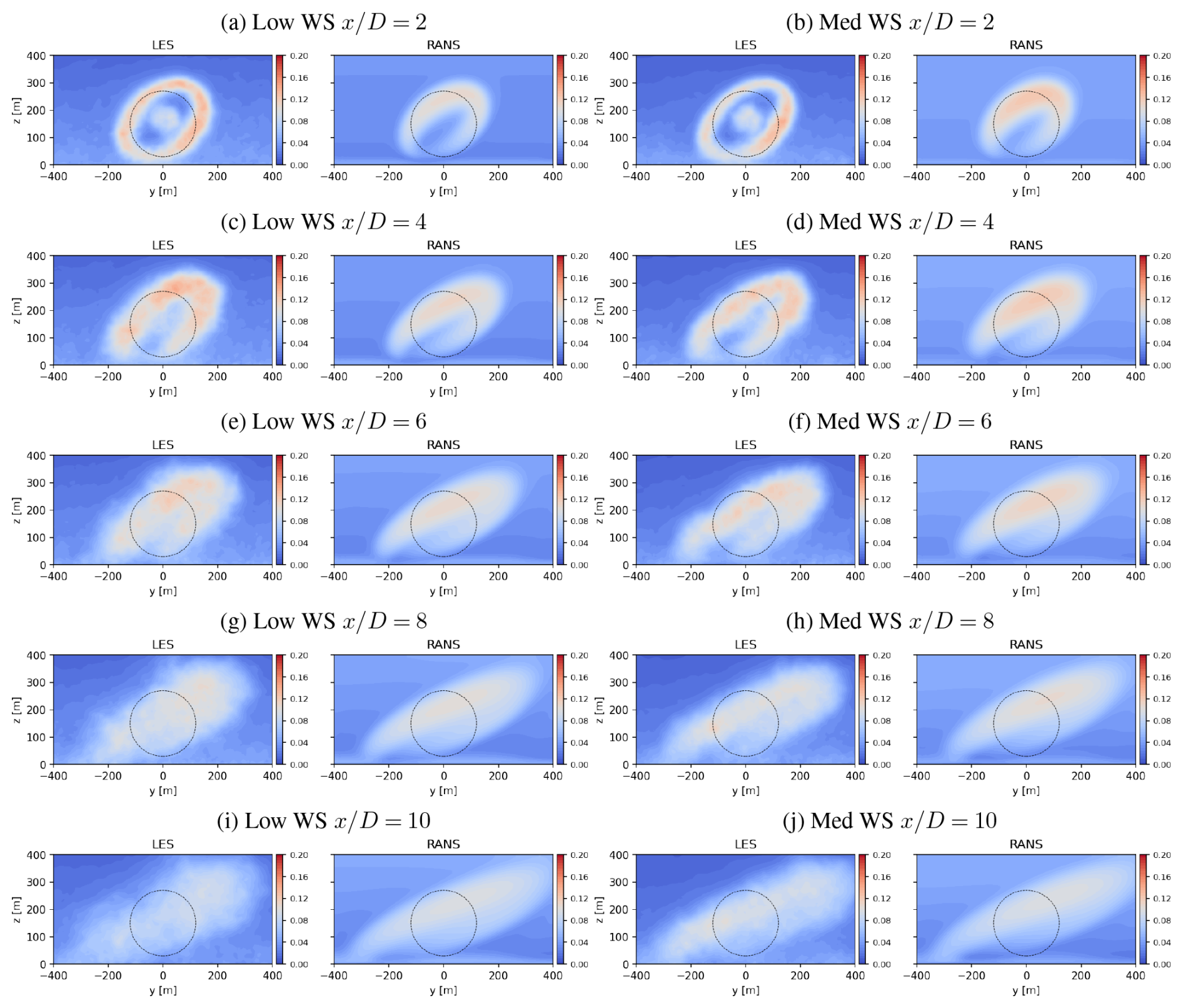
Figure 6 Comparison of the normalized turbulent kinetic energy for low- and med-WS inflow conditions, as computed by the Kynema-SGF LES and SANDWake3D RANS methods. Contours of non-dimensionalized TKE are plotted at distances $x/D=\mathrm{2}$, 4, 6, 8, and 10 downstream of the turbine. The dashed circle corresponds to the location of the rotor disk of the IEA 15 MW reference turbine.

The amount of wake-generated turbulence in the single-turbine cases can be examined in both the LES and RANS models. While the resolved TKE in the Kynema-SGF calculations and the modeled TKE in the RANS model are not directly equivalent quantities, the two can provide some indication for the degree of mixing happening inside the wake. Contours of the TKE for both the low-WS and med-WS cases are shown in Fig. 6 at different distances downstream. As expected, the TKE distribution generally aligns with the regions of wake shear, and the overall magnitude and evolution of TKE in the RANS model agrees with the results from the LES calculations. Note that in these cases with both shear and veer, the TKE is less heavily concentrated near the lower surface, which might explain the persistence of the wake deficit at lower elevations.

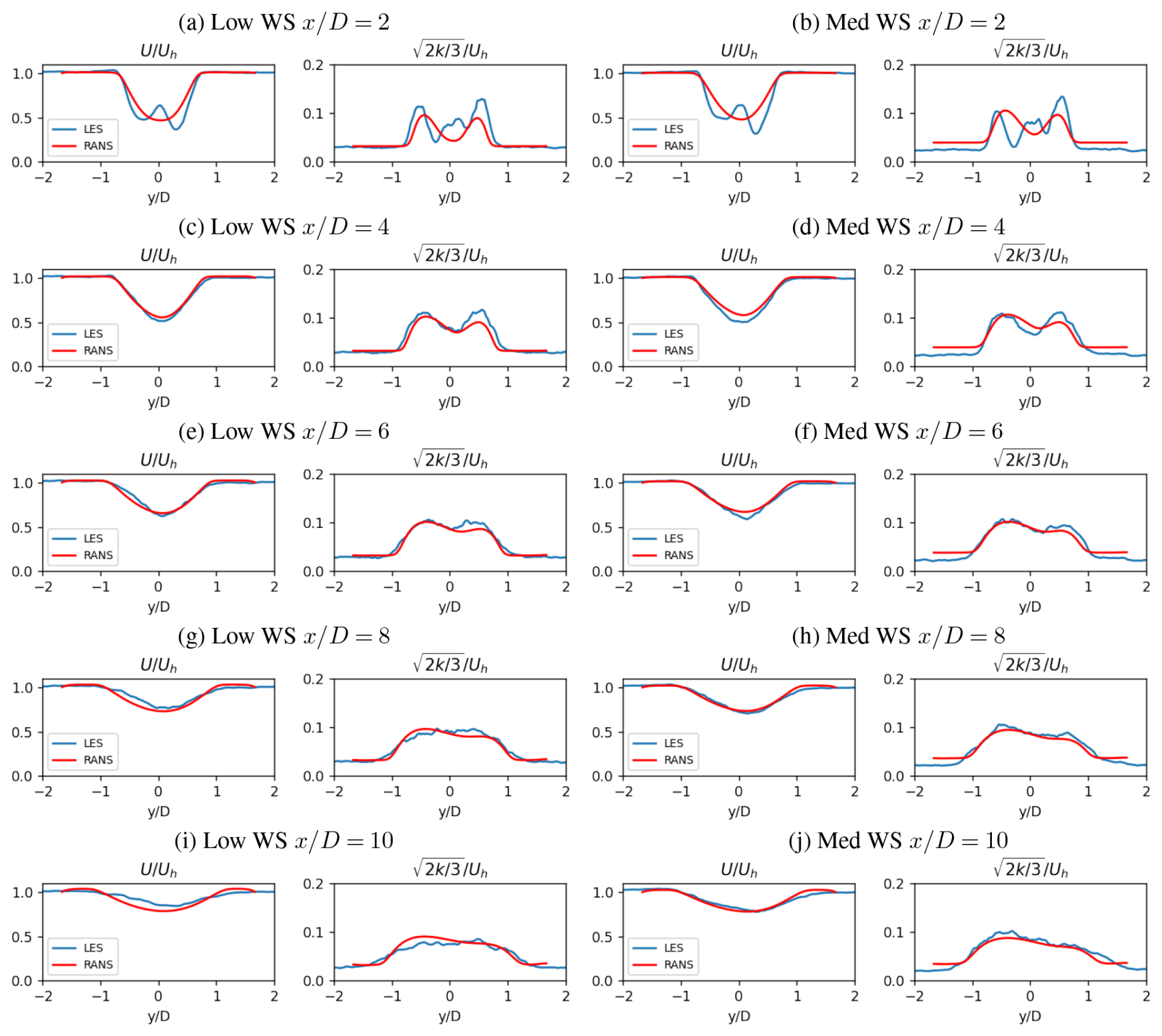
Figure 7 Hub-height profiles of the normalized velocity and normalized TKE $\sqrt{\mathrm{2}k/\mathrm{3}}/U_{\mathrm{h}}$ for the single-turbine wake under low-WS and med-WS ABL conditions, as computed by the Kynema-SGF LES and SANDWake3D RANS codes.

A more quantitative assessment of the RANS wake model is presented in Fig. 7 for both the low-WS and med-WS scenarios. In those figures, the hub-height velocity and TKE profiles are plotted for both the LES and RANS solutions. Downstream of the near-wake region, the normalized velocity profiles show good agreement between the two solution methods. While the peak values of the TKE profile are underestimated in the RANS model, the overall magnitude and distribution of the wake added turbulence are well captured by SANDWake3D.

Figure 8 (a) Definition of the wake skew angle ϕ. Downstream evolution of the wake skew ϕ(x) for the (b) low-WS and (c) med-WS case.

Also of particular interest is the examination of the behavior of the wake skew angle in the different wake models. Here, the wake skew angle is calculated using the vertical angle of the wake's major axis, as defined by the locations of the maximum wake deficit at the upper- and lower-rotor-tip heights (Fig. 8). As expected, this skew angle is nearly constant and close to 90° at all distances downstream for all of the FLORIS calculations. In the parabolic RANS approach, we see that the skew angles monotonically decrease in the downstream direction, and this trend is well captured when compared to the LES calculations for the med-WS case. The same trend is present in the low-WS case, although the RANS result is shifted compared to the LES. In the near-wake region, both the RANS and LES begin with similar ϕ angles, but a slower evolution of ϕ is observed in the LES data between $\mathrm{1}D\le x\le \mathrm{3}D$, resulting in an offset of approximately Δ_ϕ≈ 12°. The underlying reason behind this offset is a matter of ongoing research, but the overall trends are consistent in the parabolized RANS model.

4.2 Convective onshore case

In addition to the stable offshore conditions discussed in Sect. 4.1, the turbine wake from a convectively unstable ABL inflow was also considered. The inflow conditions are identical to the slightly convective ABL case described in the ExaWind benchmark repository (US Department of Energy, 2026), with a hub-height velocity of 11.4 m s⁻¹ and no appreciable veer over the rotor disk. While this case was not included in the calibration process, the same values of C_μ, C_1ϵ, and C_2ϵ from Sect. 2.5 are used to test their general applicability. A value of C_k=0.40 was chosen to match the inflow turbulence level at hub height. As shown in Fig. 9, the inflow velocity and veer profiles from the parabolized RANS approach agree well with the Kynema-SGF LES profiles.

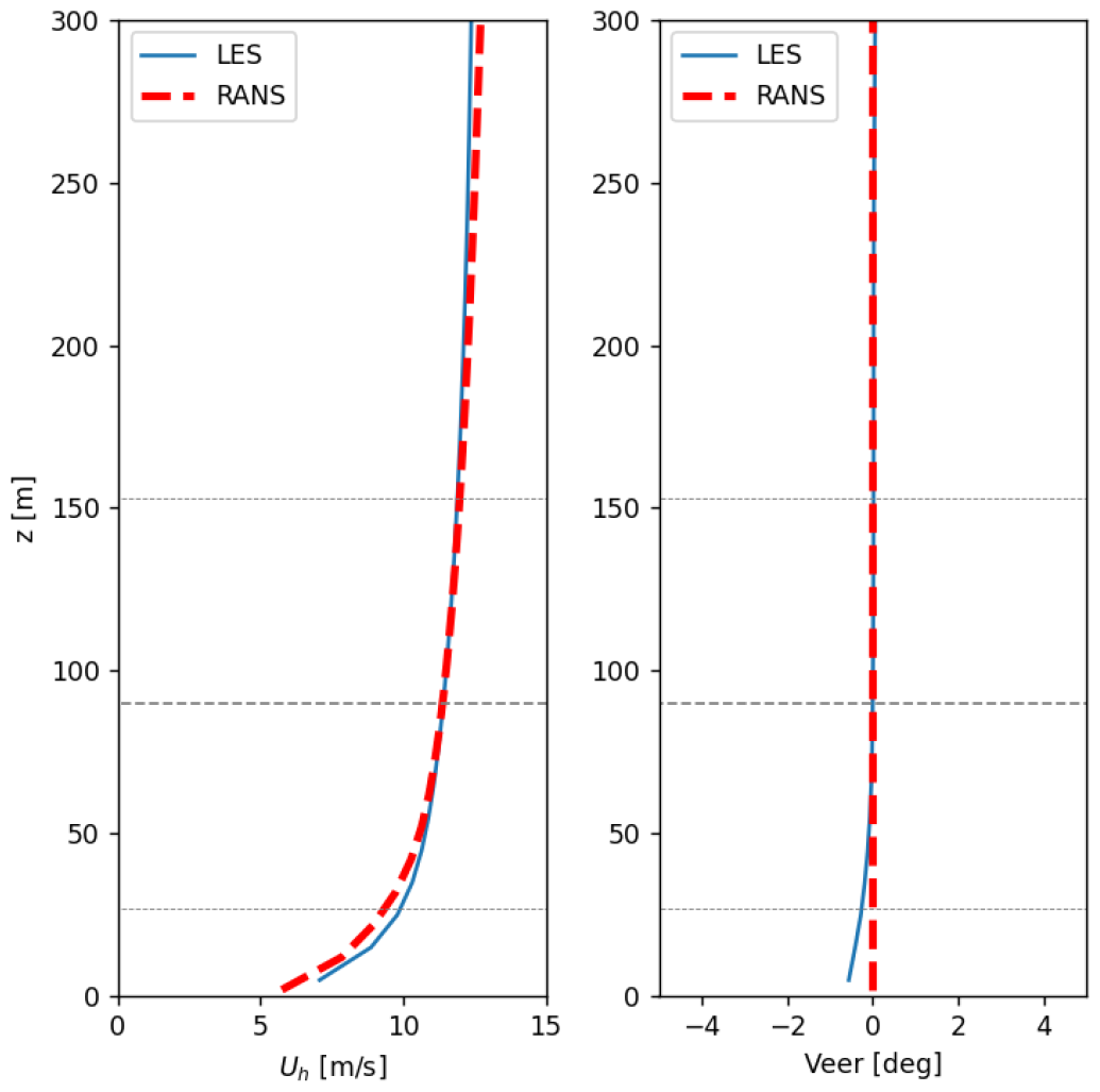
Figure 9 Comparison of the inflow horizontal velocity and veer profiles for the onshore convective ABL case in Sect. 4.2.

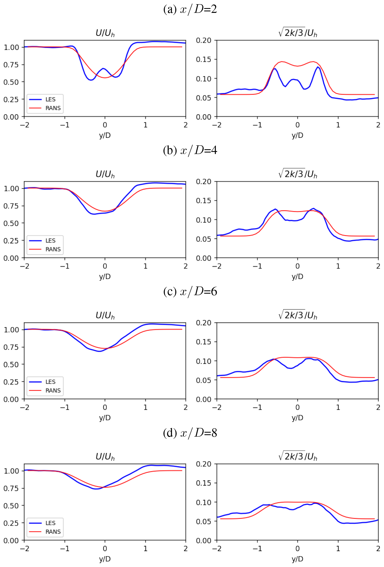
Figure 10 Comparison of the normalized hub-height velocity and turbulent kinetic energy wake profiles for the onshore convective ABL case with the NREL 5 MW turbine.

The turbine used in this case is the NREL 5 MW reference turbine, with a hub height of 90 m and a rotor diameter of 126 m, and in the Kynema-SGF LES simulation it was run with a fixed rotor speed of 12.1 rpm and a fixed blade pitch of 0°. A comparison of the hub-height velocity and TKE profiles between the LES and SANDWake3D calculations is shown in Fig. 10. Similar to the results of Sect. 4.1, the evolution of the wake deficit and width is well captured by the parabolized RANS approach. Note that the LES wake profiles show evidence of lateral asymmetry due to the presence of large-scale structures in the flow which are not modeled in RANS. The downstream TKE profiles also show similar agreement between the two methods, particularly for the downstream locations $x/D>\mathrm{2}$.

4.3 Two-turbine offshore case

Additional simulations were carried out using the SANDWake3D model on a two-turbine configuration and evaluated against the counterpart Kynema-SGF calculations. In this case, a second IEA 15 MW reference turbine was placed 5D downstream of the first IEA 15 MW turbine in the med-WS ABL conditions. This matches the two-turbine configuration studied in previous works (Frederik et al., 2025) and allows the accuracy of the wake and turbulence superposition capabilities of the parabolic RANS model to be assessed against higher-fidelity models.

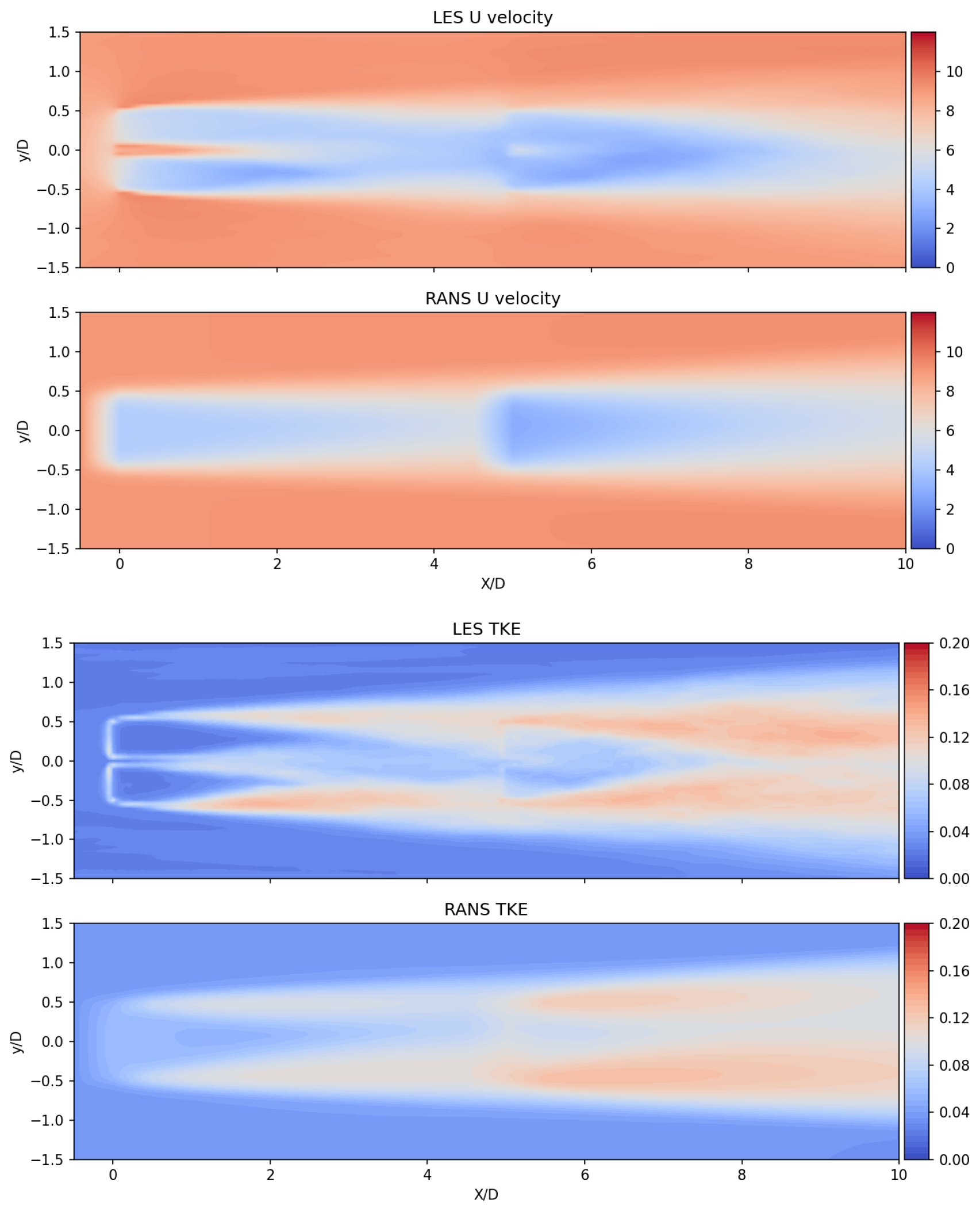
Figure 11 The streamwise velocity (top) and normalized TKE $\sqrt{\mathrm{2}k/\mathrm{3}}/U_{\mathrm{h}}$ (bottom) on the hub-height plane for the two-turbine configuration. Note that all streamwise distances are measured from the upstream turbine at $x/D=\mathrm{0}$, and the second turbine is located at $x/D=\mathrm{5}$.

Hub-height contours of the time-averaged velocity and TKE between the Kynema-SGF LES and SANDWake3D RANS model are shown in Fig. 11. Due to the parabolic nature of the problem, the RANS results upstream of x=5D remain unchanged, but the inclusion of the second turbine still resulted in very favorable comparisons with the LES without any additional adjustments of the calibration coefficients or changes to the boundary conditions. From the hub-height velocity contour comparisons, the qualitative behavior of the wake deficit and wake spread of the downstream turbine wake matches the LES calculations. Similarly, the distribution and magnitude of TKE in the downstream wake predicted by the RANS model generally matches the resolved TKE computed by Kynema-SGF.

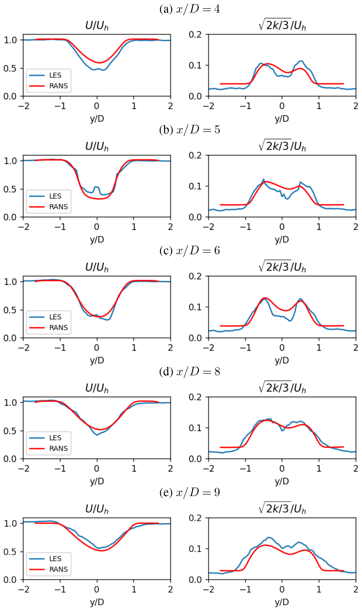
Figure 12 Hub-height profiles of the normalized velocity and TKE for the two-turbine configuration under med-WS ABL conditions, as computed by the Kynema-SGF LES and SANDWake3D RANS codes. Note that all streamwise distances are measured from the upstream turbine at $x/D=\mathrm{0}$, and the second turbine is located at $x/D=\mathrm{5}$.

A more quantitative comparison of the hub-height velocities and TKE is provided in Fig. 12. Of particular interest are the hub-height and velocity profiles close to the second turbine location and farther downstream in the second wake. Within the first diameter of the second rotor, at x=5D–6D, both the velocity and TKE profile are well captured, and the centerline differences immediately downstream of the nacelle region are not as pronounced as in the single-turbine comparisons. The increase in the RANS wake added turbulence at x=6D due to the presence of the second turbine also agrees well with the LES calculations. Farther downstream, the RANS wake profiles continue to show good agreement with the LES profiles. However, the RANS TKE profiles at x=8D–9D underpredict the peak magnitude of wake-added turbulence, although the general distribution still qualitatively agrees.

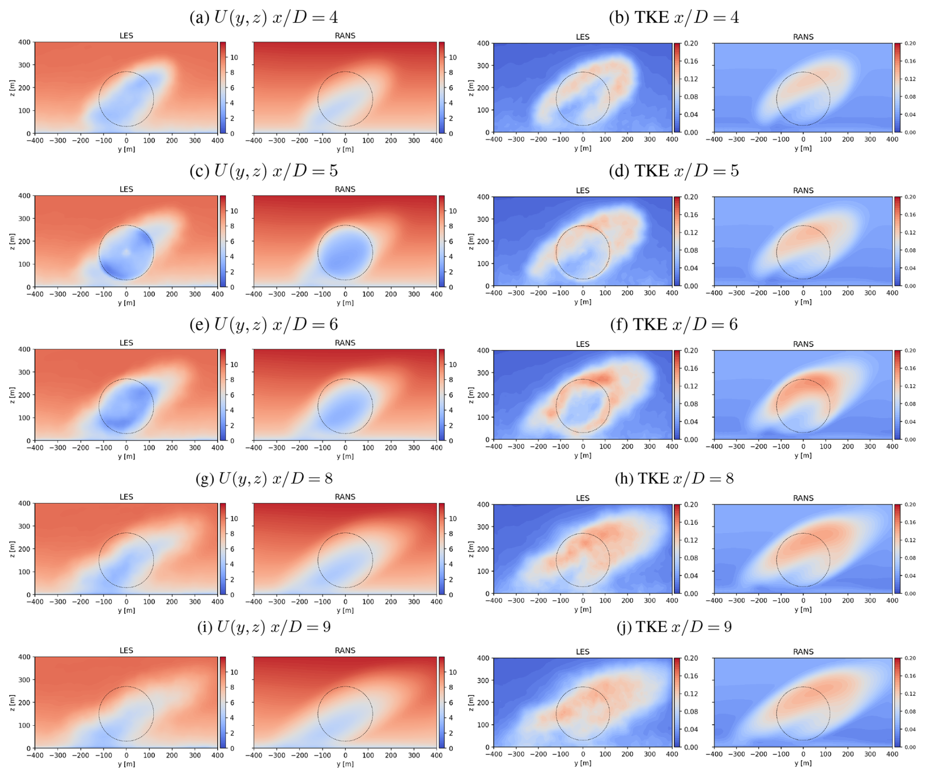
Figure 13 Rotor plane contours of the streamwise velocity and normalized TKE $\sqrt{\mathrm{2}k/\mathrm{3}}/U_{\mathrm{h}}$ for the two-turbine configuration in the med-WS inflow. Note that all streamwise distances are measured from the upstream turbine at $x/D=\mathrm{0}$, and the second turbine is located at $x/D=\mathrm{5}$.

The three-dimensional nature of the downstream wake evolution is shown in Fig. 13. Within the first diameter downstream of the second turbine, at x=5D–6D, the interaction of the second turbine wake with the skewed wake from the first turbine is well represented using the current parabolic RANS approach. Farther downstream at x=8D–9D, the eventual merging of both wakes into a single skewed wake is also consistent between the LES and RANS models. From Fig. 13, the evolution of TKE in the second wake using the parabolic RANS model also matches the observed TKE distribution from the Kynema-SGF LES results, although the peak turbulence values are stronger in the LES.

4.4 Wind farm case

In the last demonstration of the RANS model's capabilities, we simulated a nine-turbine wind farm configuration using both SANDWake3D and Kynema-SGF. This configuration matches a case studied by Yalla et al. (2025) and involves a three-row wind farm in the 9 m s⁻¹ med-WS inflow scenario, with IEA 15 MW reference turbines spaced 5D in both the lateral and streamwise directions. The full LES domain was 10 km × 10 km, while the RANS domain was approximately 4 km × 4 km. The computational expense of the simulations was approximately 86 400 GPU-h and 4 CPU-min, respectively, for the LES and RANS methods.

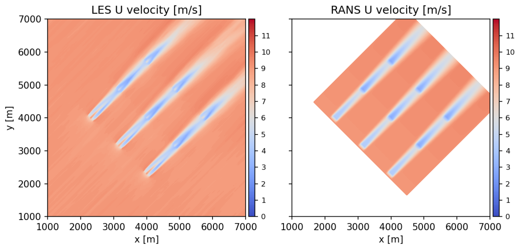
Figure 14 The streamwise velocity on the hub-height plane for the three-row turbine wind farm configuration in the med-WS inflow, as computed by the Kynema-SGF LES and SANDWake3D RANS methods. The nine IEA 15 MW turbines are spaced 5D apart in both the lateral and streamwise directions.

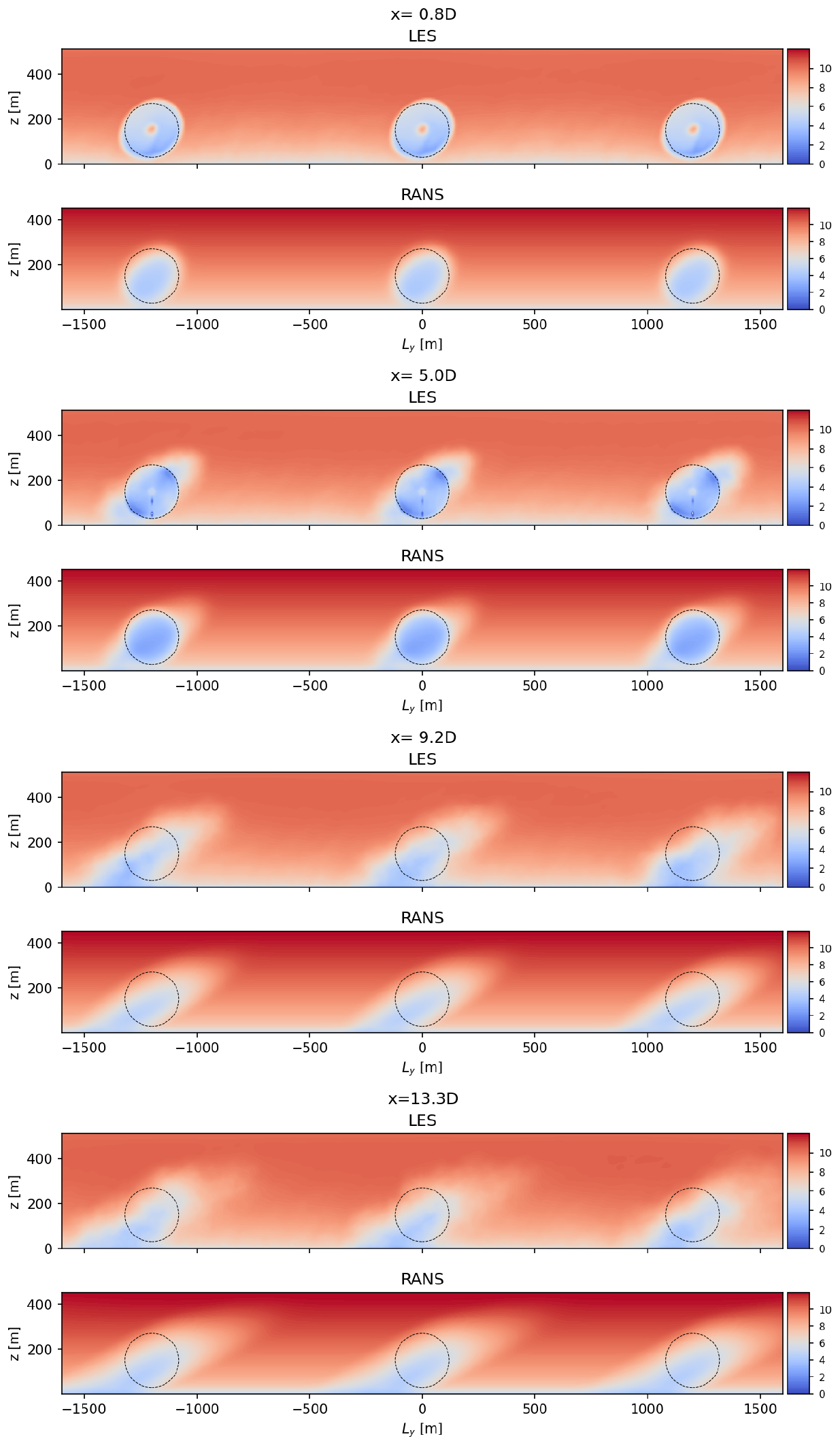
Figure 15 Rotor plane contours of the streamwise velocity, in m s⁻¹, for the nine-turbine wind farm configuration in the med-WS inflow. Note that all streamwise distances are measured from the first turbine row at $x/D=\mathrm{0}$, the second turbine row is located at $x/D=\mathrm{5}$, and the third is located at $x/D=\mathrm{10}$. Note that L_y is the lateral coordinate measured from the center turbine.

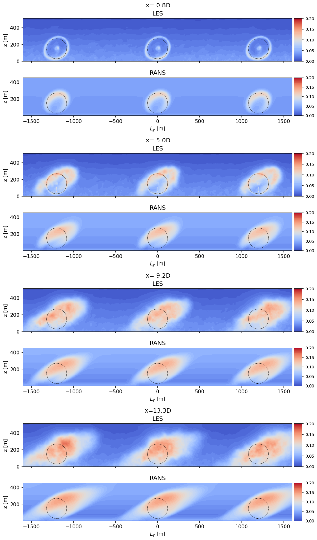
Figure 16 Rotor plane contours of the normalized TKE $\sqrt{\mathrm{2}k/\mathrm{3}}/U_{\mathrm{h}}$ for the nine-turbine wind farm configuration in the med-WS inflow. Note that all streamwise distances are measured from the first turbine row at $x/D=\mathrm{0}$, the second turbine row is located at $x/D=\mathrm{5}$, and the third is located at $x/D=\mathrm{10}$. Note that L_y is the lateral coordinate measured from the center turbine.

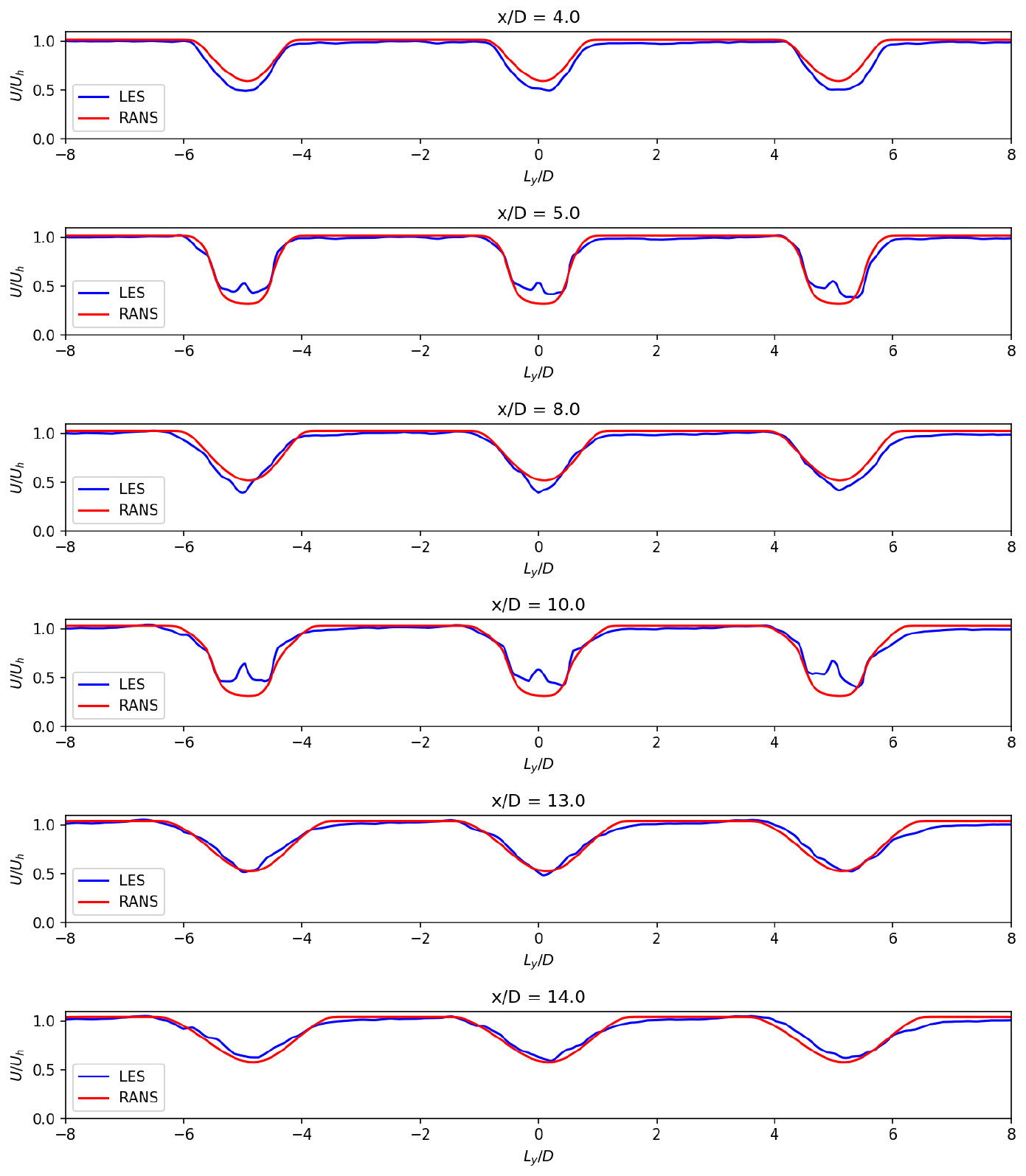
Figure 17 Hub-height profiles of the normalized velocity for the nine-turbine wind farm configuration under med-WS ABL conditions, as computed by the Kynema-SGF LES and SANDWake3D RANS codes. Note that all streamwise distances are measured from the first turbine row at $x/D=\mathrm{0}$, the second turbine row is located at $x/D=\mathrm{5}$, and the third is located at $x/D=\mathrm{10}$. Note that L_y is the lateral coordinate measured from the center turbine.

A qualitative comparison of the solutions is provided in Figs. 14–16. From the hub-height comparisons of the streamwise velocity in Fig. 14, we see that the general wake spread and wake deficit magnitudes are captured by the RANS model. The effects of veer on the second- and third-row wakes are shown in Fig. 15, and the behavior is consistent with the earlier observations in Sects. 4.1 and 4.3. Downstream of the third row, the wake skew and stretching in both codes appears to evolve more slowly compared to the wake from the first turbine row. Similar behavior for the rotor plane TKE can be seen in Fig. 16, and the comparison of the hub-height velocity profiles in Fig. 17 shows the general agreement between the RANS and LES approaches. Additional work is ongoing regarding the study of the RANS-modeled wakes in complex wind farm configurations, and the results will be reported in future studies.

4.5 Joukowski actuator disk comparisons

More complex wake features can be captured in SANDWake3D by using more sophisticated actuator disk models. As an example, we consider the Joukowski constant circulation actuator disk model as formulated by Sørensen et al. (2020). This model captures both the veer–swirl interactions and near-wake behavior by including the azimuthal velocity distributions and the blade root loading corrections. A complete description of the model can be found in Sørensen et al. (2020) and is briefly summarized below.

In this model, the axial force f_x and azimuthal force f_θ on the rotor disk are defined as

$$\begin{array}{}\text{(25a)}& {\displaystyle }& {\displaystyle }{f}_x=\mathit{\rho }{u}_{\mathit{\theta }}\left(\mathrm{\Omega }r+{\displaystyle \frac{u_{\mathit{\theta }}}{\mathrm{2}}}\right)\text{(25b)}& {\displaystyle }& {\displaystyle }{f}_{\mathit{\theta }}=\mathit{\rho }{u}_D{u}_{\mathit{\theta }},\end{array}$$

where Ω is the rotor speed, and u_D=u_D(r) is the axial velocity in the plane of the rotor. The azimuthal velocity distribution u_θ=u_θ(r) on the rotor is modeled as an actuator disk with constant circulation modified with a tip correction and a root correction. By providing the rotor speed Ω and thrust coefficient C_T as a function of the wind speed, Eqs. (25a) and (25b)can be solved to determine the torque, power, and thrust of the wind turbine, as well as the forces f_x and f_θ on the rotor disk. While additional inputs are required to use this actuator disk model compared to the uniformly loaded model of Sect. 2.4, the computational efficiency of the SANDWake3D calculations remains largely unchanged. Initial results using the Joukowski disk model also make use of the same RANS calibration parameters mentioned in Sect. 2.5, although additional calibration should be performed in future studies to widen its generality.

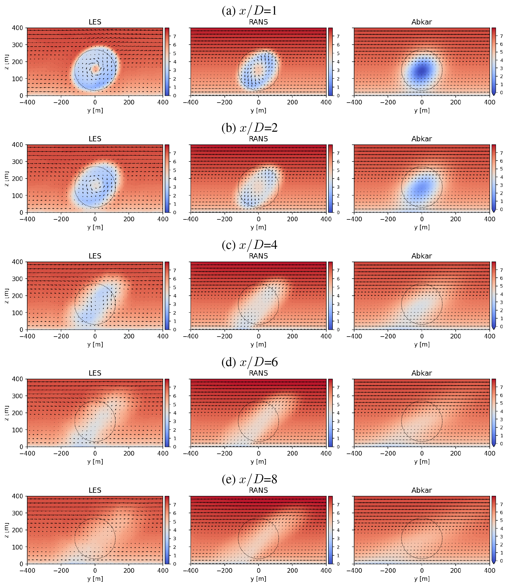
Figure 18 Comparison of the streamwise velocity for the low-WS case computed by the LES, RANS, and semi-analytic approach of Abkar et al. (2018). Contours of u(y,z) are plotted with units of m s⁻¹ at distances $x/D=\mathrm{1}$, 2, 4, 6, and 8 downstream of the turbine. The dashed circle corresponds to the location of the rotor disk of the IEA 15 MW reference turbine.

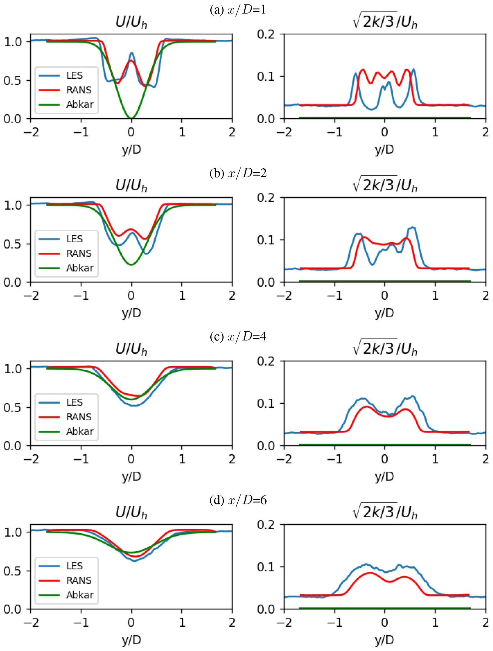
Figure 19 Hub-height profiles of the normalized velocity and normalized TKE $\sqrt{\mathrm{2}k/\mathrm{3}}/U_{\mathrm{h}}$ for the single-turbine wake under low-WS ABL conditions, as computed by the LES, SANDWake3D RANS, and Abkar et al. (2018) model.

The wake resulting from the Joukowski actuator disk model can be compared to the semi-analytic Gaussian model of Abkar et al. (2018). The results for the single-turbine low-WS scenarios are shown in Figs. 18 and 19 and highlight the differences between the two wake models. In the near-wake region, the lower loading near the blade root leads to the formation of a small high-velocity region near the centerline. This is present in both the LES and the SANDWake3D calculations, but absent in the Abkar et al. (2018) model, which uses a Gaussian wake deficit velocity profile that is not applicable in the near-wake region. The presence of the tangential forces in the LES and the RANS models also leads to the presence of an azimuthal swirl velocity in the near-wake fields. This swirl–veer interaction leads to a lateral asymmetry in the wake velocity deficit profile, as shown in Fig. 19a and b. These effects are not included in the Abkar et al. (2018) model as it only calculates the axial wake velocity deficit. Also note that the SANDWake3D model with the Joukowski actuator disk model also provides qualitatively similar turbulence behavior in the wake compared to the LES, but no turbulence information is provided in the semi-analytic Gaussian model.

Table 5 Comparison of computational cost for the simulation of a single-turbine wake. Note that the Kynema-SGF simulations were performed on the Frontier Exascale 1600 GPU supercomputer. n/a: not applicable.

5 Discussion

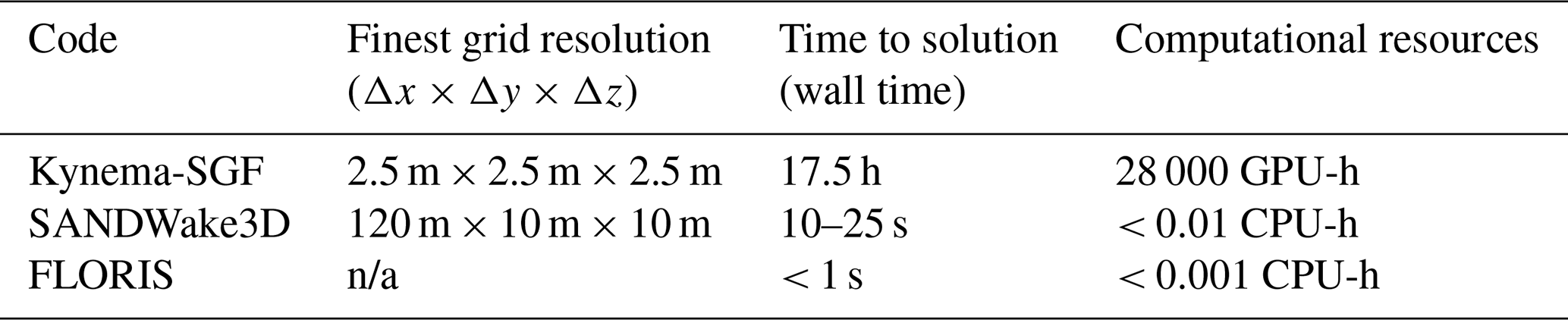
During optimization studies for wind farm layouts and control strategies, tens or hundreds of thousands of flow solutions are typically required (Thomas et al., 2023). Related to the three simulation tools examined herein, the computational costs, and thus the feasibility for performing such studies, vary greatly, as shown in Table 5. It is notable that while the RANS solution's computational expense is closer to that of an engineering wake model like FLORIS, its realism is comparable to that of the high-fidelity LES solution including (quantitatively validated) effects of veer and shear. Thus, the RANS approach embodied by SANDWake3D offers a unique balance between prediction accuracy and computational efficiency that can enable better design and optimization of wind farms.

6 Conclusions

This study demonstrated an efficient, three-dimensional wake model which combines the parabolic k−ϵ RANS equations with an atmospheric boundary layer model and an actuator disk model for representing turbine rotors. This RANS model, known as SANDWake3D, can naturally incorporate complex effects such as shear, veer, atmospheric stratification, and wake superposition. By using an ADI scheme the numerical solution for the three-dimensional wake behavior can be found quickly using orders of magnitude fewer computational resources than traditional RANS or LES methods. The results of the SANDWake3D RANS model were compared to equivalent Kynema-SGF LES calculations for stable-ABL conditions at two different wind speeds. In the single-turbine wakes, a similar degree of wake stretching and skewing was observed in both the RANS and LES calculations, and SANDWake3D was also able to capture the wake deficit behavior. The distribution of wake added turbulence showed excellent agreement between the two calculation methods. In the comparisons for the two-turbine configuration, the SANDWake3D model was able to handle the wake superposition behavior without difficulty and also captured the corresponding increase in wake turbulence.

There are several improvements and generalizations that are possible topics for future studies. The current work demonstrates the potential of the parabolized k−ϵ for stably stratified ABL conditions, but a similar calibration and validation process can be applied to neutral and unstable ABL flows. The computational performance of SANDWake3D can also be further optimized to decrease solution times for large-wind-farm applications. The current implementation is serial, and additional speed increases may be possible by considering multi-processor parallelization or using GPU optimizations. For large-wind-farm cases, using a domain decomposition approach can also lead to much faster computations.

In addition to performance enhancements, the uniformly loaded actuator disk model described in Sect. 2.4 can also be replaced with other actuator disk models, such as those using blade element momentum theory. Coupling with wind turbine control models would also allow different wind farm optimization strategies to be tested. This would allow interactions between veer and swirl to be included in future wake simulations. Similarly, the effects of yaw misalignment and wake steering on wake behavior are also naturally included in this formulation and can be the subject of future studies. Lastly, to model the behavior of active wake mixing controls in turbine wakes, a linear stability model can be incorporated into SANDWake3D, similar to the approach of Cheung et al. (2025).

Future work may also improve on the current parabolized RANS solution by superimposing the turbine induction solution ahead of each rotor position. One possibility is to calculate the induction field using Green's function approach of Cheung et al. (2024a) and correcting the upstream solution for any slowdown or acceleration effects. To increase the general applicability of the RANS model, calibration against a wider range of atmospheric conditions, including wind speed, TI, and stratification, should also be carried out. Additional work may also focus on using alternate inflow profiles, rather than profiles derived from Monin–Obukhov similarity theory. This may allow more complex atmospheric inflows to be considered, including those with low-level jets, temperature inversion layers, and other such phenomena.