Offshore wind profile characteristics and their impact on floating wind turbine power production

In this study, we investigate the impact of vertical wind shear and wind speed inversions on the power production of a floating offshore wind turbine. Using nacelle-mounted wind lidar data from a 6 MW turbine at the Hywind Scotland wind farm, we analyse inflow conditions and turbine performance during summer and autumn. The wind climatology shows that 33 % of examined cases exhibit non-standard wind profiles within the rotor-swept area, including negative shear and wind speed inversions. These conditions can significantly affect power production. In particular, in the below-rated wind speed range, we find differences ranging from 5 % to 10 % between wind profile cases with negative and positive shear. Our findings demonstrate that deviations from the logarithmic wind profile at the operating height range of modern offshore wind turbines can introduce substantial bias in a power curve verification procedure, with differences up to 20 % compared to a reference power curve of a fixed-bottom wind turbine. Nacelle-mounted wind lidars provide critical insight into the inflow offshore characteristics, enabling improved performance assessment of floating offshore wind turbines. The results highlight the need for an implementation of measurement strategies that capture wind conditions across the full rotor-swept area.

1 Introduction

Offshore wind conditions offer significant potential for renewable energy production. Sea surface characteristics, such as low friction and high spatial homogeneity, result in wind conditions typically characterized by low atmospheric turbulence levels and high spatial isotropy. These conditions favour the development of large wind turbines with high power production capacity. However, as the operating height of wind turbines increases, the wind field they interact with may exhibit a vertical profile with negative shear or wind speed inversion. These features can occur, for example, in a shallow atmospheric boundary layer or in the presence of a low-level jet (LLJ) (Peña et al., 2008; Hallgren et al., 2023). These wind conditions are relevant for the operation of offshore wind farms, as they can affect wind turbines both in terms of power production and aerodynamic loads (Gutierrez et al., 2017; Doosttalab et al., 2020; Gadde and Stevens, 2021; Paulsen et al., 2026). Until today, it is still challenging to predict the characteristics of these wind profile events using mesoscale and reanalysis (e.g. Nunalee and Basu, 2014; Bui et al., 2025; Olsen et al., 2025), which highlight the need for more observational studies of offshore wind profiles (Shaw et al., 2022).

Measuring offshore wind conditions is a challenging task. The depth of the ocean floor makes the installation of meteorological masts technically demanding and costly. For this reason, tall (≥100 m) offshore masts equipped with in situ wind sensors are currently installed only at few locations (e.g. the FINO – research platforms in the North Sea and Baltic Sea (FINO, 2025), and the meteorological mast in the Inch Cape Offshore Wind Farm). The height range of meteorological masts can be extended through the use of remote-sensing ground-based wind profilers, which can be installed on fixed (e.g. Peña et al., 2008; Kim et al., 2019; Schepers et al., 2021; Bui et al., 2025) and floating (e.g. Foussekis and Mouzakis, 2021) platforms that support masts. A paradigm shift in measuring offshore wind profiles was introduced with the development of floating wind lidar profilers, i.e. Doppler lidars installed on buoys (Gottschall et al., 2017). Floating wind lidars have been shown to measure mean wind speed at different heights accurately (e.g. Peña et al., 2022) and thus used to study offshore wind profiles (e.g. Debnath et al., 2021).

A promising option for expanding the wind energy sector, despite the need for further technological developments (Robertson et al., 2025), is floating offshore wind turbines (FOWTs). However, assessing the operation of this concept is challenging, as it relies on the interaction between ambient wind conditions, sea state, and the corresponding motion induced in a FOWT during operation. FOWTs experience motion in 6 degrees of freedom while operating: three rotational (roll, pitch, and yaw) and three translational movements (surge, sway, and heave). Currently, there is increasing interest within the wind energy research community in assessing the impact of the motions induced on a FOWT during operation on power production (e.g. Couto et al., 2022; Fontanella et al., 2024). This topic has been primarily investigated through wind tunnel experiments and computational fluid dynamics simulations. Due to the complexity of this problem, researchers usually decouple the FOWT motions and investigate their impact separately (e.g. Sant et al., 2015; Wen et al., 2017; Li et al., 2018; Wen et al., 2018a, b; Fu et al., 2019). However, to date, only a few studies have examined the power production of utility-scale FOWTs operating in natural atmospheric and sea-state conditions (e.g. Özinan et al., 2022). Thus, it is still unclear how the motions over 6 degrees of freedom, coupled with the wind profile characteristics, affect the power production of a FOWT.

The study of a utility-scale wind turbine's power production is based on the power curve verification (PCV) procedure described by the International Electrotechnical Committee (IEC 61400-12-1, 2022). Offshore wind conditions tend to reduce complications in performing PCV compared to onshore, as the sea state can be considered spatially homogeneous. However, as discussed above, variations in the vertical wind speed gradient at the top of the rotor create a need to observe the wind profile not only at hub height but also across a wide range of altitudes spanning the rotor plane. In general, the impact of shear on power production has been identified in onshore fixed-bottom wind turbines for the case of vertical wind speed variations close to the ground (Wagner et al., 2009). For this reason, especially in those cases where the vertical variations of wind speed deviates from a height-dependent logarithmic profile, it is recommended to use a rotor-equivalent wind speed (REWS) (Wagner et al., 2011). The use of nacelle-mounted wind lidars, which operate while mounted on a wind turbine's nacelle, offers great potential for performing PCV for mainly two reasons. First, the optical axis of nacelle-mounted wind lidars, i.e. the axis relative to which the geometry of the line-of-sight measurements is defined, follows the yaw direction of the nacelle, thus maximizing data availability (Wagner et al., 2014b). Second, nacelle-mounted wind lidars provide measurements at different heights and radial distances, they are necessary for the estimation of a REWS. Furthermore, nacelle-mounted wind lidars that include a levelled line of sight parallel to the yaw direction can provide estimations of the turbulence intensity of the wind (Peña et al., 2017; Guo et al., 2026), a parameter that can introduce uncertainties in a PCV. This makes nacelle-mounted wind lidars an alternative option to floating wind lidars for offshore measurements, in the context of a PCV. A general complication in performing a PCV using a nacelle-mounted wind lidar is that, in the case where measurements acquired at different distances from the rotor are used to parameterize the inflow conditions, the impact of the induction zone of the wind turbine should be taken into consideration. Furthermore, performing a PCV using a nacelle-mounted wind lidar to a FOWT is challenging since the optical axis of the wind lidar is subject to floater dynamics, and therefore a motion-correction procedure is required to correct the wind lidar measurements (Gräfe et al., 2023).

Nacelle-mounted wind lidars provide a practical means of characterizing the inflow to large offshore wind turbines (e.g. Angelou et al., 2023; Vratsinis et al., 2025; Fang et al., 2026). However, their wind field reconstruction methods may not adequately capture complex vertical wind profiles that occur under natural atmospheric conditions. The first objective of this study is therefore to assess how well simple parameterizations, such as constant vertical gradient of the wind shear and veer across the rotor, reproduce the observed wind profile and to determine whether discrepancies are linked to LLJs. To achieve this objective, we analyse summer and autumn measurements from a nacelle-mounted wind lidar installed on a FOWT at Hywind Scotland, the world's first commercial floating offshore wind farm (Jacobsen and Godvik, 2021), located in the North Sea off the east coast of Scotland, which is a region of high offshore wind-energy potential (Hahmann et al., 2023). The wind lidar observations enable the study of the offshore wind profile characteristics at the northern North Sea. In addition to atmospheric conditions, FOWT motions can influence performance. At Hywind Scotland, turbines' rotor mean tilt varies with operating conditions, providing a unique opportunity to investigate its impact on power production. Therefore, the second objective of this study is to evaluate the FOWT power curve using a motion-corrected nacelle-mounted wind lidar and to examine whether deviations can be attributed to rotor tilt and wind profile characteristics.

In Sect. 2.1, we describe the field campaign and the measurement configuration of the wind lidars and the data post-processing steps. In Sect. 3, we present a model that expresses the wind lidar measurements as a function of wind profile characteristics. This model is used to study the inflow conditions of the FOWT. Finally, in Sect. 4, we present our results on wind profile characteristics and their impact on the power production of the FOWT. The implications of these results are discussed in Sect. 5.

2 Material and methods

2.1 Floating offshore wind turbine

The wind turbine examined in this study is one of five floating offshore wind turbines (FOWTs) that form the Hywind Scotland wind farm. The wind turbine positions (labelled HS1, HS2, HS3, HS4, and HS5) are arranged in a W-shaped configuration, rotated 30° clockwise relative to true north, as illustrated in Fig. 1. The configuration is described within a right-handed coordinate system, where the y axis is oriented towards the north; and the origin is defined at the location of the HS4 turbine, which is the one used in this study. The FOWTs (SWT-6.0-154, Siemens Gamesa Renew. Energ.) have a hub height of 98.6 m and a rotor diameter of D=154 m. They are mounted on floating platforms based on a ballasted spar buoy concept and have been operating since 2017 (Jacobsen and Godvik, 2021). Below the rated wind speed, blade pitch is regulated in the same manner as in a conventional bottom-fixed wind turbine. Above the rated wind speed, however, the blade pitch control operates in coordination with the floater motion control system.

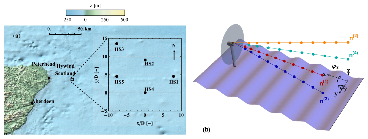
Figure 1 (a) Map of Scotland's eastern coastline indicating the offshore Hywind Scotland wind farm location (black rectangle). A schematic of the wind farm layout, comprising five turbines (labelled HS1, HS2, HS3, HS4, and HS5), represented in a right-handed coordinate system with the y axis oriented towards the north and the origin located at the HS4 turbine. (b) Schematic of the wind turbine showing the four nacelle-mounted Doppler lidar line-of-sight directions (n) and the coordinate system used to describe rotations about the x and y axes, corresponding to nacelle pitch and roll rotations.

The most notable motion experienced by the wind turbines during operation occurs along the pitch axis, with angles ranging from 0 to 7° at wind speeds between cut-in and rated (Angelou et al., 2023). Above the rated wind speed, the pitch angle decreases until it reaches a mean value close to 2°. Less significant variations are observed in the roll angle, which on average ranges between 0 and 0.5° for wind speeds between cut-in and rated. In contrast to the pitch angle, the roll angle continues to increase above rated speed, reaching approximately 1°. When comparing the magnitude of the mean pitch and roll angles, the roll angle is 60 %–90 % smaller than the pitch angle. In addition to the mean rotation about the pitch and roll axes, the operation of the Hywind Scotland turbines is characterized by wind-speed-dependent dynamic rotations around the yaw, pitch, and roll axes (Jacobsen and Godvik, 2021). The standard deviation of the yaw and roll angles follows a similar trend, increasing with hub-height wind speed and reaching a maximum of about 0.8 and 0.4°, respectively. In contrast, the maximum standard deviation of the pitch (i.e. 0.8°) occurs near the rated wind speed, while at lower and higher wind speeds the standard deviation of the pitch is less than 0.4°. Furthermore, the magnitude of the dynamic motion of the Hywind Scotland turbines depends on atmospheric stability, with lower dynamic motion in all yaw, pitch, and roll rotations observed under stable conditions (Jacobsen and Godvik, 2021). Overall, the observed mean and dynamic pitch motion indicates that the Hywind Scotland wind turbines tilt away from the wind in a stable manner, as the standard deviation of the pitch angle remains small. This is not necessarily the case for other floater types. For example, Gräfe et al. (2023) reports FOWT pitch angles with a lower mean magnitude but higher dynamic fluctuations.

2.2 Wind lidar

The inflow wind conditions experienced by the HS4 wind turbine were monitored using a nacelle-mounted Doppler lidar. The Doppler lidar (Wind Iris Turbine Control, Vaisala Oyj) acquires radial wind speed measurements along four separate lines of sight. The direction of each line of sight is defined by a three-dimensional unit vector $\mathit{n}=\mathit{\{}{n}_{\mathrm{1}},n_{\mathrm{2}},n_{\mathrm{3}}\mathit{\}}$, with azimuth angles of −15 or +15° and tilt angles of −5 or +5°, relative to the instrument's optical axis (see Figs. 1 and 2). Radial wind speeds are acquired at 10 distances from the lidar: 50 m (0.32D), 80 m (0.52D), 120 m (0.78D), 160 m (1.04D), 200 m (1.30D), 240 m (1.56D), 280 m (1.82D), 320 m (2.08D), 360 m (2.34D), and 400 m (2.60D) – all distances measured along the optical axis of the Doppler lidar. The sampling rate of 0.25 Hz results in 150 measurements per range gate per a 10 min period. The transceiver of the lidar was tilted by 2.5° relative to a levelled nacelle. Although the Wind Iris is a fixed-pattern-scanning¹ Doppler lidar, its installation on a FOWT caused the measurement geometry, in relation to a fixed coordinate system, to be distorted by turbine motion. When the turbine tilt angle reaches 5°, corresponding to hub-height wind speeds between 8.5–9.5 and 12.5–13.5 m s⁻¹, the lidar configuration consists of two beams that are nearly horizontal and two beams measuring across the upper part of the rotor (see Fig. 2a). In this configuration, the three farthest range gates of the lower beams and the four farthest range gates of the upper beams are located outside the rotor plane (see Fig. 2b).

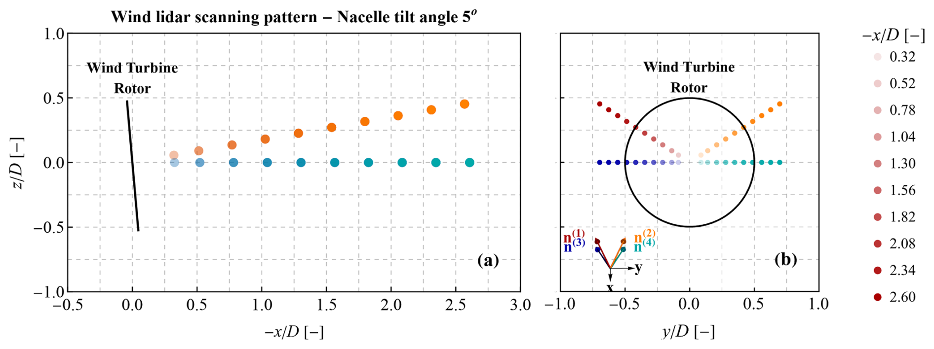
Figure 2 Scanning pattern of the nacelle-mounted wind lidar when the tilt of the floating offshore wind turbine is equal to 5°, corresponding to the wind speed ranges 8.5–9.5 and 12.5–13.5 m s⁻¹. The two lower beams (denoted as n⁽³⁾ and n⁽⁴⁾) are almost horizontal when the pitch angle is approximately equal to 5°. The x axis is parallel to the yaw direction and pointing downwind.

2.3 Data

The wind turbine was instrumented with a motion reference unit (MRU) installed on the nacelle to monitor its mean and dynamic responses. The MRU measures the pitch and roll angles of the nacelle, corresponding to rotations about the longitudinal and transverse axes relative to the turbine's yaw direction. Data from the MRU were logged alongside active power and wind speed measurements from a nacelle-mounted anemometer via the supervisory control and data acquisition (SCADA) system at 1 Hz. Unlike the other parameters, the yaw direction was recorded only when changes occurred. Based on the sampling rate of the Doppler lidar data, a complete set of radial wind speed observations for all lines of sight was available every 4 s. Synchronization between the two data acquisition systems was verified by comparing the internal accelerometer readings of the Doppler lidar with those from the MRU in the nacelle.

In this study, we examine data from January 2019 to October 2020. The dataset does not cover the entire period but includes three intervals: 1–30 January 2019, 1 September–29 November 2019, and 1 June–1 October 2020. Discontinuities were due either to missing turbine data or periods when the nacelle-mounted lidar was not operating. Overall, the dataset contains SCADA measurements equivalent to approximately 6 months.

To avoid including cases in which wakes from adjacent turbines distorted the inflow conditions at the HS4 turbine, only data acquired during turbine operation with yaw directions between 90 and 270° were selected, resulting in 13 247 10 min periods of SCADA data. The wind lidar data were filtered based on the data availability at each range gate. Only periods with at least 50 % data availability were selected, which reduced the initial wind lidar data set by 10 % to 17 057 10 min periods. The SCADA data were post-processed to estimate statistics synchronized with the wind lidar measurements. However, concurrent lidar and SCADA data were available for only 6729 periods. Additionally, some periods exhibited large yaw standard deviations. To focus on stable wind directions, only periods where the yaw standard deviation within a 10 min interval was ≤ 10° were retained. Applying this criterion resulted in a dataset of 6659 cases (i.e. 10 min periods). The selected dataset represents climatological conditions typical of summer and autumn.

3 Wind profile parameterization

To study the inflow conditions, we examine the mean radial wind speed across the four lines of sight and derive parameters describing the vertical profile at the upper part of the wind turbine rotor. For this purpose, we define first a three-dimensional coordinate system with its origin at the nacelle-mounted wind lidar, and the x axis is horizontal, aligned with the turbine's yaw direction and pointing downwind. Second, we consider that the wind vector U is described by three components: u, v, and w. Subsequently, we assume that the free inflow, undisturbed by the presence and operation of the wind turbine, is horizontally homogeneous, such that the wind vector U at a position with coordinates $\mathit{\{}x,y,z\mathit{\}}$ satisfies $U\left(x,y,z\right)=U\left(z\right)$. The inflow conditions are characterized by parameterizing the vertical profile as a function of (i) the longitudinal ${\stackrel{\mathrm{‾}}{u}}_{\mathrm{\infty }}$ and transverse ${\stackrel{\mathrm{‾}}{v}}_{\mathrm{\infty }}$ mean components of the free wind vector U at the nacelle height (the overbar denotes mean quantities) and (ii) the vertical gradients of these components (i.e. ${\displaystyle \frac{\partial \stackrel{\mathrm{‾}}{u}}{\partial z}}$ and ${\displaystyle \frac{\partial \stackrel{\mathrm{‾}}{v}}{\partial z}}$).

Furthermore, we adopt the assumptions about inflow along the rotor plane described in Angelou et al. (2023), namely (i) the two horizontal mean wind components $\mathit{\{}\stackrel{\mathrm{‾}}{u},\stackrel{\mathrm{‾}}{v}\mathit{\}}$ at a given height are spatially homogeneous along the y axis, (ii) the vertical wind component is negligible ($\stackrel{\mathrm{‾}}{w}=\mathrm{0}$ m s⁻¹), and (iii) the gradients ${\displaystyle \frac{\partial \stackrel{\mathrm{‾}}{u}}{\partial z}}$ and ${\displaystyle \frac{\partial \stackrel{\mathrm{‾}}{v}}{\partial z}}$ within the vertical range of the nacelle-mounted lidar's measurement area are constant with height. Using these assumptions, and considering that the distortion of the inflow wind speed along the x axis (induced by turbine operation) can be represented as a function of an induction factor (Medici et al., 2011; Simley et al., 2016), we express the four line-of-sight measurements v_r of the nacelle-mounted wind lidar as

$$\begin{array}{}\text{(1)}& \begin{array}{rl}& \left(\begin{array}{c}{v}_r^{\left(\mathrm{1}\right)}\\ v_r^{\left(\mathrm{2}\right)}\\ v_r^{\left(\mathrm{3}\right)}\\ v_r^{\left(\mathrm{4}\right)}\end{array}\right)=-\mathbf{M}\left(\begin{array}{c}{\stackrel{\mathrm{‾}}{u}}_{\mathrm{\infty }}\\ \frac{\partial \stackrel{\mathrm{‾}}{u}}{\partial z}\\ {\stackrel{\mathrm{‾}}{v}}_{\mathrm{\infty }}\\ \frac{\partial \stackrel{\mathrm{‾}}{v}}{\partial z}\end{array}\right),\\ & \text{where}\mathbf{M}=\\ & \left(\begin{array}{cccc}& \mathrm{⋮}& & \\ n_{\mathrm{1}}^{\left(i\right)}{f}_{\mathrm{ind}}\left(n_{\mathrm{1}}^{\left(i\right)}{d}_f\right)& n_{\mathrm{1}}^{\left(i\right)}{n}_{\mathrm{3}}^{\left(i\right)}{d}_f{f}_{\mathrm{ind}}\left(n_{\mathrm{1}}^{\left(i\right)}{d}_f\right)& n_{\mathrm{2}}^{\left(i\right)}& n_{\mathrm{2}}^{\left(i\right)}{n}_{\mathrm{3}}^{\left(i\right)}{d}_f\\ & \mathrm{⋮}& & \end{array}\right)\end{array}\end{array}$$

is the matrix of the line-of-sight unit vectors ${\mathit{n}}^{\left(i\right)}=\mathit{\{}{n}_{\mathrm{1}}^{\left(i\right)},n_{\mathrm{2}}^{\left(i\right)},n_{\mathrm{3}}^{\left(i\right)}\mathit{\}}$, where i=1, 2, 3, and 4 correspond to each of the four line-of-sight directions. The direction of the vectors n are dependent on the system-defined azimuth and tilt angles of lines of sight, and on the pitch and roll angles of the nacelle. Furthermore, in Eq. (1), d_f is the distance from the instrument to the measurement volume, and f_ind is a function that describes the reduction of the free wind speed in the induction zone of the wind turbine. This parameterization is commonly used to express nacelle-mounted wind lidar observations as a function of wind conditions (Borraccino et al., 2017; Angelou et al., 2023). Each measurement in the Wind Iris dataset is tagged with the corresponding upwind distance x_f, reported as the nominal horizontal distance from the instrument along the x axis. The actual distance d_f can be computed by multiplying x_f by the norm of the vector $\mathit{\{}\mathrm{1},\tan \mathit{\varphi },\tan \mathit{\theta }\mathit{\}}$, where ϕ and θ correspond to the azimuth and elevation angles of the lines of sight, respectively. The reduction of longitudinal wind speed along a line normal to the rotor centre, as described by vortex sheet theory (Conway, 1995; Medici et al., 2011), is expressed by the induction factor a. This factor adequately describes the evolution of wind speed as it approaches a turbine rotor, as demonstrated in a field test by Simley et al. (2016) for an onshore wind turbine, using the following formula:

$$\begin{array}{}\text{(2)}& f_{\mathrm{ind}}\left(x\right)=\mathrm{1}-a\left(\mathrm{1}+{\displaystyle \frac{\mathit{\zeta }}{\sqrt{\mathrm{1}+{\mathit{\zeta }}^{\mathrm{2}}}}}\right),\end{array}$$

where $\mathit{\zeta }=-x-x_{\mathrm{L}}/R$ is the distance normalized by the rotor radius R=77 m, x_L is the distance between the rotor plan and nacelle-mounted lidar (i.e. 4 m), and a is the induction factor.

Based on the considerations above, the wind vector in the top part of the rotor can be expressed as

$$\begin{array}{}\text{(3)}& \mathit{U}(x,z)=\mathit{\left\{}\right({\stackrel{\mathrm{‾}}{u}}_{\mathrm{\infty }}+{\displaystyle \frac{\partial \stackrel{\mathrm{‾}}{u}}{\partial z}}\cdot z\left)f_{\mathrm{ind}}\right(x),{\stackrel{\mathrm{‾}}{v}}_{\mathrm{\infty }}+{\displaystyle \frac{\partial \stackrel{\mathrm{‾}}{v}}{\partial z}}\cdot z,\mathrm{0}\mathit{\}}.\end{array}$$

The model presented in Eq. (1) is applied to all measurements, including the farthest range gates located outside the rotor plane (see Fig. 2b). The reason is that for the farthest range gates (i.e. >2D), we do not expect a significant impact of induction zone on the radial wind speeds. Furthermore, the estimation of the induction factor in Eq. (2) remains unchanged even when considering its radial distribution, for example, by using the empirical model of Troldborg and Meyer Forsting (2017) which considers the radial distance in the parameterization of the induction factor a. The performance of the model of Eq. (1) in estimating the upwind mean wind speed characteristics is assessed by calculating the root mean square error (RMSE), hereafter denoted as ε_u between the modelled (Eq. 1) and measured radial wind speeds for each 10 min period using all range gates along the four different line-of-sight directions.

3.1 Vertical wind profile

Based on the radial speed measurements acquired at a height z but from different lines of sight, it is possible to estimate the longitudinal and transverse components of the wind vector. For this calculation, an estimation of the induction factor a of the wind turbine is required. The two horizontal wind components are then equal to

$$\begin{array}{}\text{(4)}& \begin{array}{rl}& u_{\mathrm{\infty }}\left(z\right)={\displaystyle \frac{n_{\mathrm{2}}^{\left(j\right)}{v}_r^{\left(i\right)}-n_{\mathrm{2}}^{\left(i\right)}{v}_r^{\left(j\right)}}{f_{\mathrm{ind}}\left(n_{\mathrm{1}}{d}_f\right)(-n_{\mathrm{1}}^{\left(j\right)}{n}_{\mathrm{2}}^{\left(i\right)}+n_{\mathrm{1}}^{\left(i\right)}{n}_{\mathrm{2}}^{\left(j\right)})}}\text{and}\\ & v_{\mathrm{\infty }}\left(z\right)={\displaystyle \frac{-n_{\mathrm{1}}^{\left(j\right)}{v}_r^{\left(i\right)}+n_{\mathrm{1}}^{\left(i\right)}{v}_r^{\left(j\right)}}{-n_{\mathrm{1}}^{\left(j\right)}{n}_{\mathrm{2}}^{\left(i\right)}+n_{\mathrm{1}}^{\left(i\right)}{n}_{\mathrm{2}}^{\left(j\right)}}},\end{array}\end{array}$$

where the superscripts i and j denote the index of two line-of-sight vectors over which radial speeds are acquired at height z, and n₁ and n₂ are the two horizontal components of the line-of-sight vectors. The pitch and the roll angle of the nacelle of the FOWT are considered for the determination of line-of-sight vector n. Equation (4) is used to reconstruct the wind profile at the top part of the rotor.

4 Results

4.1 Modelling the radial speed of the Doppler lidar

The first objective of this study was to assess how well the radial speed model presented in Eq. (1) reproduces the trends observed in the lidar data. Figure 3 shows the mean radial speeds for each line of sight during four separate 10 min periods, all characterized by the same hub-height wind speed (8 m s⁻¹). Each case represents different inflow conditions and corresponds to periods where lidar measurements were available for all 10 range gates along each line of sight. Figure 3a illustrates the simplest wind conditions: a positive gradient of u $\left({\displaystyle \frac{\partial \stackrel{\mathrm{‾}}{u}}{\partial z}}>\mathrm{0}\right)$ and negligible gradient of v $\left({\displaystyle \frac{\partial \stackrel{\mathrm{‾}}{v}}{\partial z}}\sim \mathrm{0}\right)$. The radial speed model (solid lines), based on the assumption of constant velocity vertical gradients, adequately describes the observations (dots). In general, when the turbine yaw is aligned with the wind direction, the two lower beams measure the same line-of-sight velocity at any distance. Vertical shear results in higher radial speeds for the upper beams compared to the lower beams, while vertical veer causes relative high values of ${\displaystyle \frac{\partial \stackrel{\mathrm{‾}}{v}}{\partial z}}$ which leads to larger differences between the upper beams' radial speeds because wind direction changes with height. This effect is evident in Fig. 3b, where the wind veer causes the wind direction to change by 18° between hub height and blade tip height. Agreement between observations and the radial speed model is not limited to cases of positive shear. An example is shown in Fig. 3c, where negative shear at the top of the rotor results in lower radial speeds for the upper beams compared to the lower ones. Even when shear is zero, differences between upper and lower beams are expected due to the tilt angle affecting the projection of the horizontal wind vector on the upper beam's line of sight, typically resulting in a 1.5 %–2.5 % difference. However, the observed differences range from 5 % to 20 %, depending on the upper beam and measurement range, which indicate the presence of negative shear. In all three cases, a clear reduction in radial wind speed is observed at around 160 m (∼1D) towards the rotor, caused by turbine operation. This reduction corresponds to high induction factors (0.38–0.41), consistent with velocity deficits in the wake when the turbine operates at below-rated wind speed (Angelou et al., 2023). Similar high induction factors have been reported by Larsen and Hansen (2014), who investigated the aerodynamic induction of a full-scale wind turbine using two scanning Doppler lidars.

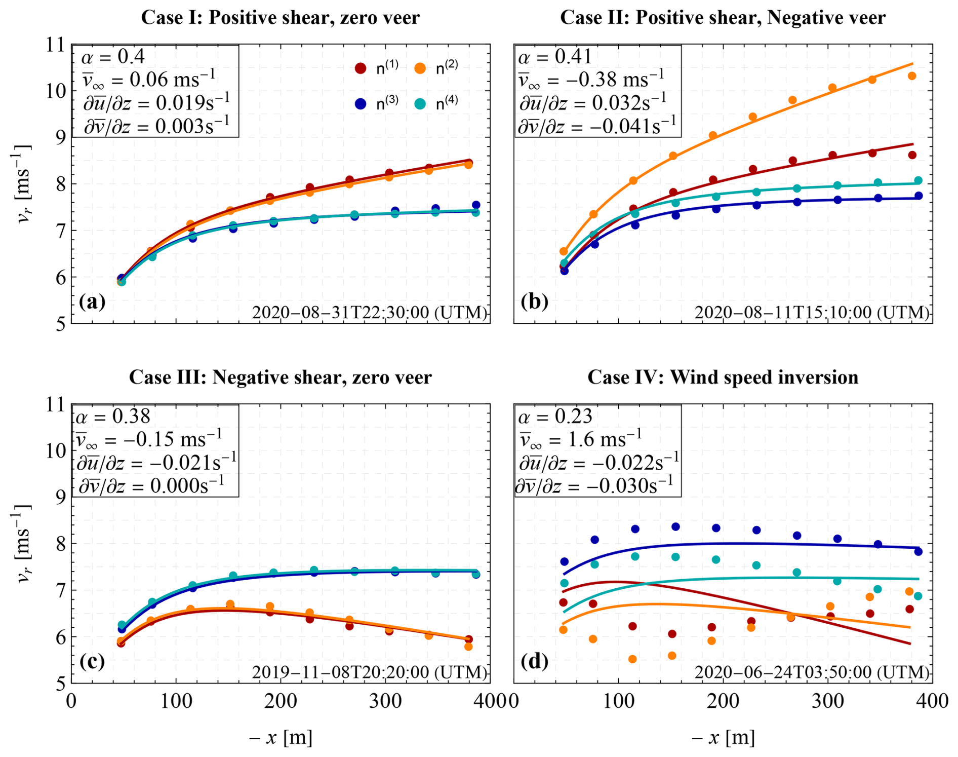
Figure 3 Example of the mean radial speed measurements (presented in dots) of a nacelle-mounted wind lidar acquired over four different lines of sight (i.e. n⁽ⁱ⁾, with i=1, 2, 3, and 4) and upwind distances (i.e. 50–400 m) during 10 min periods when the wind profile was characterized by positive ${\displaystyle \frac{\partial \stackrel{\mathrm{‾}}{u}}{\partial z}}$ and zero ${\displaystyle \frac{\partial \stackrel{\mathrm{‾}}{v}}{\partial z}}$ (a), positive ${\displaystyle \frac{\partial \stackrel{\mathrm{‾}}{u}}{\partial z}}$ and negative ${\displaystyle \frac{\partial \stackrel{\mathrm{‾}}{v}}{\partial z}}$ (b), negative ${\displaystyle \frac{\partial \stackrel{\mathrm{‾}}{u}}{\partial z}}$ and zero ${\displaystyle \frac{\partial \stackrel{\mathrm{‾}}{v}}{\partial z}}$ (c), and by wind speed inversion (d). The information of the upwind conditions $\left({\stackrel{\mathrm{‾}}{v}}_{\mathrm{\infty }},{\displaystyle \frac{\partial \stackrel{\mathrm{‾}}{u}}{\partial z}}\text{and}{\displaystyle \frac{\partial \stackrel{\mathrm{‾}}{v}}{\partial z}}\right)$ and the induction factor a of the wind turbine of each example is presented in the corresponding plot. The solid lines correspond to the estimated distribution of the line-of-sight velocities using Eq. (1).

In contrast to the good agreement observed in Fig. 3a–c, which corresponded to cases where the RMSE ε_u of Eq. (1) has values of less than 0.2 m s⁻¹, 11 % of the examined 10 min periods show that the inflow model could not reproduce the trends in the lidar data (see Fig. 3d). This discrepancy is attributed to wind profiles with wind speed inversions, as occurs in LLJs. In such cases, simplified parameterizations of the vertical wind profile (i.e. constant shear and veer coefficients) cannot predict the observed radial speed distribution.

4.2 Wind profile characteristics

The analysis of wind profile characteristics was conducted only for 10 min periods, where the model in Eq. (1) performed adequately. These cases were identified by inspecting the RMSE ε_u between the inflow model and the 10 min mean radial speeds. Values above 0.2 m⁻¹ were considered unsatisfactory for representing the spatial distribution of the lidar measurements. This threshold was empirically chosen and corresponds to mean absolute differences of less than 5 % between hub-height wind speed measurements from the nacelle-mounted lidar and the turbine anemometer (Angelou et al., 2023). As already stated in the previous section, based on this criterion, 757 cases (11 % of the dataset) were excluded. As shown in Fig. 3d, these cases are likely associated with the presence of LLJs. A similar occurrence of LLJs (approximately 12 %) during spring and summer months was reported in an offshore field campaign in the North Sea by (Kalverla et al., 2017). During these events, the turbine yaw direction spanned a sector from 90 to 256°, indicating that the observed LLJs were not caused by flow crossing a coastal-sea interface.

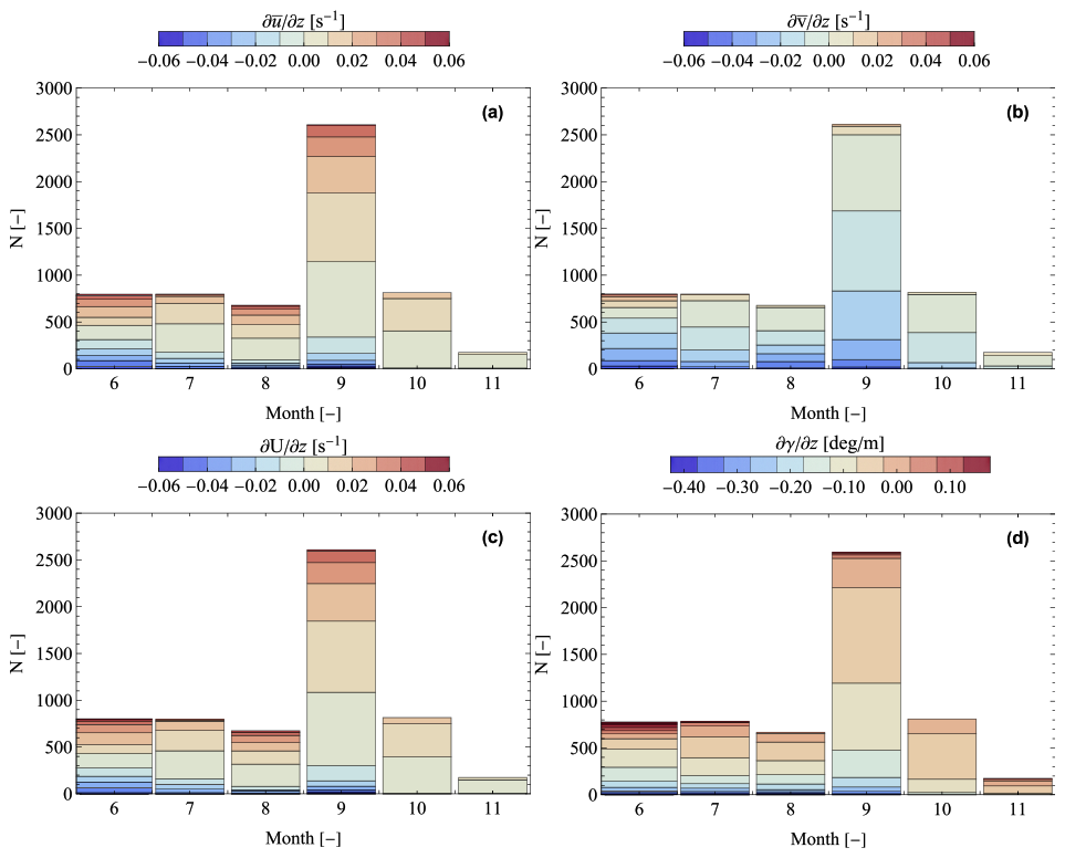
Figure 4 Bar chart of the distribution of the estimated gradients (a) ${\displaystyle \frac{\partial \stackrel{\mathrm{‾}}{u}}{\partial z}}$ and (b) veer ${\displaystyle \frac{\partial \stackrel{\mathrm{‾}}{v}}{\partial z}}$ along with the corresponding shear (c) and veer (d) of the wind profile along the top part of the wind turbine rotor for different 10 min periods over different months.

Figure 4a and b present a bar chart of the estimated wind speed gradients for each month using Eq. (1). The values of ${\displaystyle \frac{\partial \stackrel{\mathrm{‾}}{u}}{\partial z}}$ within the height layer corresponding to the upper section of the FOWT rotor range from −0.06 to 0.06 s⁻¹ (Fig. 4a). The vertical gradient of the transverse wind component ${\displaystyle \frac{\partial \stackrel{\mathrm{‾}}{v}}{\partial z}}$ is generally found to be negative, as expected in the location of the FOWT (Fig. 4b), with the higher values having been observed in cases where the gradient ${\displaystyle \frac{\partial \stackrel{\mathrm{‾}}{u}}{\partial z}}$ is strong. Using the estimated values of the vertical gradients of the wind components, we compute the shear and veer of the wind profile by estimating the horizontal wind speed and direction at the hub height and at the top of the rotor, which are presented in Fig. 4c and d. Periods with negative shear are found during the months from June to September and account for 22 % of the dataset, a percentage similar to that reported by Furevik and Haakenstad (2012), who studied wind profile characteristics over the North Sea. These profiles, which may include LLJs, typically occur in areas with variations in topography (Tuononen et al., 2015). For negative shear cases, it remains unclear whether the core of an LLJ is found within the lower half of the rotor or if a wind speed inversion occurs at very low heights, as has been observed in the North Sea (Furevik and Haakenstad, 2012). When focusing on data acquired between June and September, negative shear does not consistently occur when the wind originates from a specific sector. Only during July and September is negative shear observed in a narrow wind direction sector between 200 and 250°. These values appear in at least one 1 h period on 13 d in July and almost every day (i.e. 30 d) in September. In contrast, during June and August, negative shear is not associated with a specific wind direction sector but occurs across the entire selected sector (90–270°), as shown in Appendix A. The observed negative shear values are independent of the time of day.

4.3 Case study: wind profile with a low-level jet

To further investigate wind profiles with negative shear and/or wind speed inversions, we examine as a case study a 12 h period between 08:40 and 20:40 on 26 June 2020. Figure 5a shows the corresponding wind conditions. The figure presents the mean horizontal wind speed U_∞ at different heights, corresponding to the magnitude of the two horizontal components (i.e. $\sqrt{{\stackrel{\mathrm{‾}}{u}}_{\mathrm{\infty }}^{\mathrm{2}}+{\stackrel{\mathrm{‾}}{v}}_{\mathrm{\infty }}^{\mathrm{2}}}$), which are calculated using Eq. (4). The estimation of these components is based on pairs of radial speed measurements acquired at different ranges and heights, and represents the spatial average over 10 m vertical layers. This period was chosen because it is characterized by vertical profiles with either negative shear or a speed inversion (highlighted in red or black, respectively, in the bar below Fig. 5a).

Figure 5 Case study of a 12 h period when the vertical wind profiles are characterized by negative shear and wind speed inversions. The time series of the vertical profile of the horizontal free wind speed (U_∞) is presented in (a). An example of one of the profiles where a wind speed inversion is observed, highlighted by a dashed rectangle in (a), is shown in (b). The characterization of each profile is visualized using black (case of negative shear), red (wind speed inversion), and white (cases of positive shear or data that are missing) in a bar below the density plot (a). The power produced by the wind turbine, normalized by the nominal value based on the power curve, is presented in (c) using either the hub-height wind speed estimated using the wind lidar (U_Hub) or the sonic anemometer (U_Nac) installed on the nacelle.

In the cases of negative shear, the wind speed decreases from hub height (98.6 m) towards the top of the rotor (∼170 m) at rates varying between 0 and −0.05 s⁻¹. On these occasions, a speed inversion occurs somewhere below hub height, but, due to the absence of measurements in the lower half of the rotor, its exact location cannot be determined. For wind profiles with a speed inversion, the profiles typically exhibit one inflection point around a maximum value. In a few cases, profiles such as that shown in Fig. 5b display two inflection points – around a maximum and a minimum – within the vertical range of 90–180 m, which form a core in the wind profile. The presence of two inflection points enables the identification of LLJs based on the difference ($\mathrm{\Delta }\stackrel{\mathrm{‾}}{U}$) between the minimum (${\stackrel{\mathrm{‾}}{U}}_{\min }$) and maximum (${\stackrel{\mathrm{‾}}{U}}_{\max }$) wind speeds. In addition to these vertical profile features, this period is noteworthy for its highly variable hub-height wind speed, ranging from 6 to 14 m s⁻¹, with a yaw direction between 140 and 180°. This makes it an interesting case for studying turbine power production under different inflow conditions. Figure 5c shows the turbine's normalized power output. The normalization is performed based on the power curve of a fixed-bottom wind turbine using the hub-height wind speed – either the wind lidar (U_Hub) or the sonic anemometer (U_Nac) installed on the nacelle. We note here that a transfer function for correcting the effect of the rotor has been applied by the wind turbine manufacturer. Deviations from nominal power reach up to 50 %, with smaller deviations observed when using the nacelle-mounted sonic anemometer as the reference wind speed. These results indicate that inflow conditions with negative shear or speed inversions can significantly impact FOWT power production. Therefore, it is important to quantify the height at which wind speed inversions occur, the magnitude of the associated speed difference, and the duration of these events. Among the entire dataset, a local maximum in the vertical wind speed profile could be detected in 10 % of the cases. Figure 6 presents (a) the wind speed difference between the maximum and minimum wind speeds within the examined height range (100–200 m), (b) the inversion height, and (c) the duration of those events. The wind speed difference was usually small (0.25–0.5 m s⁻¹), although in 10 % of the selected cases, differences greater than 2 m s⁻¹ were observed. For a slight majority of cases, the inversion height was around 130 m, but overall, the range over which inversions were observed was between 100 and 160 m. This height range is consistent with studies that have been performed in different locations in the North Sea (Rausch et al., 2022; Paulsen et al., 2026). To identify the duration of the events characterized by such wind conditions, hourly periods where at least 30 min of either velocity inversions or negative shear in the wind profile were selected. Using this criterion, we find that most profiles persist for about 60 min; however, eight periods were identified where these characteristics lasted for an extended duration (700–900 min). Similar LJ duration statistics have been reported by Olsen et al. (2025) for the wind conditions over the North Sea.

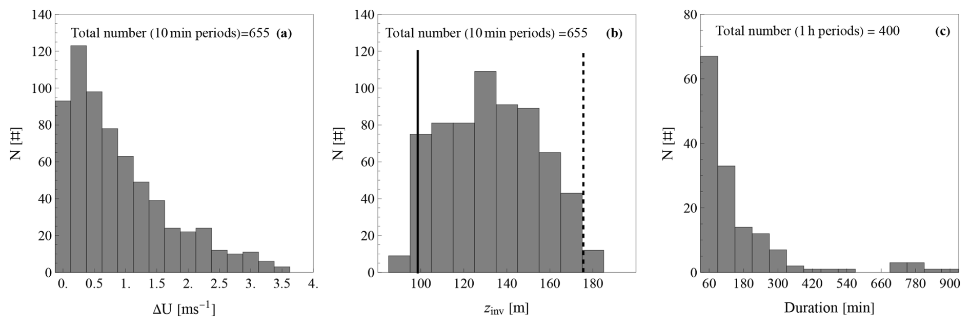
Figure 6 Histograms of (a) the wind speed difference (ΔU) between the maximum and the minimum wind speed along the wind vertical profile, (b) the height of the wind speed inversion (z_inv), and (c) the duration of periods in which either wind speed inversion or negative shear were identified. The solid and dashed vertical lines in (b) denote the hub height and top height of the rotor.

4.4 Power curve verification

The transceiver of the nacelle-mounted wind lidar was installed above the rotor centre. Consequently, Eq. (1) estimates the two components of the horizontal free wind vector at a position vertically displaced relative to hub height. To verify the installation height of the wind lidar (z_L), we calculated the mean minimum absolute difference between the hub-height wind speed reported by the nacelle-mounted anemometer and a wind speed estimated using the function ${\stackrel{\mathrm{‾}}{u}}_{\mathrm{\infty }}+{\displaystyle \frac{\partial \stackrel{\mathrm{‾}}{u}}{\partial z}}{z}_{\mathrm{L}}$. Different values of z_L were tested for all periods, ranging from −10 to 10 m in steps of 0.1 m, and the minimum difference was found when the lidar was translated vertically by 4 m. This height offset is therefore used to estimate hub-height wind speed.

In the case presented in Fig. 5, vertical wind profiles with speed inversions or negative shear at the top of the rotor are linked to a reduction in turbine power production (as a reference, we used the power curve of a bottom-fixed turbine of the same type as the FOWT examined in this study). To assess the impact of inflow conditions on FOWT power production, we performed a power curve verification (PCV) analysis. For this purpose, an accurate hub-height wind speed estimate is required. Although the range gates at 2.6D of the two lower beams are nearly horizontal at a 5° turbine pitch, the mean turbine angle places them between approximately 60 and 125 m above sea level. In addition, the mean roll angle induces a vertical displacement between the two that can reach 7 m (see Appendix B). Therefore, we examine three hub-height wind speed estimation methods that can be used in the context of a PCV:

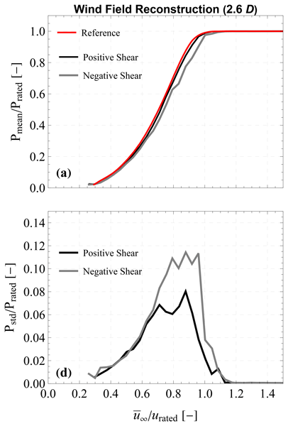
1. Wind field reconstruction (2.6D). The hub-height wind speed is calculated using Eq. (1) with measurements only at 2.6D (see Fig. 7a). Note that the nacelle pitch angle causes the measurement plane at a given distance to be tilted rather than vertical. The tilt is proportional to the nacelle pitch angle. However, because nacelle-mounted lidars typically use low-elevation angles for their lines of sight, this tilt has minimal impact on the horizontal distance from the rotor. Considering that measurements are acquired over a probe length, the horizontal displacement can be treated as negligible.

2. Wind field reconstruction (all range gates). The hub-height wind speed is calculated using Eq. (1) with all available measurements (see Fig. 7b).

3. Rotor-equivalent wind speed (REWS). The hub-height wind speed is estimated using the REWS as defined in IEC 61400-12-1 (2022). For this calculation, we assume that the wind shear estimated at the top of the rotor is representative of conditions at the bottom. Due to this assumption, REWS is calculated only for cases where positive shear is estimated using Eq. (1). For profiles with negative shear, the location of wind speed inversion in the lower rotor cannot be determined, so using the estimated parameters to compute REWS is not justified.

The purpose of testing the three wind speed estimates is to investigate how sensitive the power curve verification is to the choice of reference wind speed. In this context, power and wind speed data were grouped in 0.5 m s⁻¹ bins, and mean and standard deviation statistics of the produced power were estimated which are presented in Fig. 7. The mean power is compared to a reference power curve model of a fixed-bottom wind turbine of the same type as the one installed in Hywind Scotland. We observe a notable difference in the power curve between positive and negative wind shear conditions (Fig. 7a–b). The estimation of REWS in the case of the profiles with positive shear, shown in Fig. 7c, results in a power curve similar to those obtained using the other two hub-height wind speed definitions. Typically, using REWS reduces scatter in the power curve depending on the magnitude of wind shear (Wagner et al., 2011). For low wind shear values, only small differences are observed when REWS is applied (Wagner et al., 2014a; Van Sark et al., 2019). In our dataset, offshore wind conditions produce power curve scatter, expressed by the standard deviation of power, that is comparable across all three hub-height wind speed estimates in the cases of wind profiles with positive shear. However, a significant difference is observed in the case of negative shear profiles, where the standard deviation is nearly twice that of positive shear cases below rated speed. Here we have to note that if the estimation of the REWS was possible in the case of the wind profiles with a negative shear, then this could result in a decreased estimated value of the hub-height wind speed since an inversion would occur closer to the ground. This could lead to a closer agreement between the power curves of the positive and negative shear cases, and could explain the differences that we see in the standard deviation of the mean produced power presented in Fig. 7d and e.

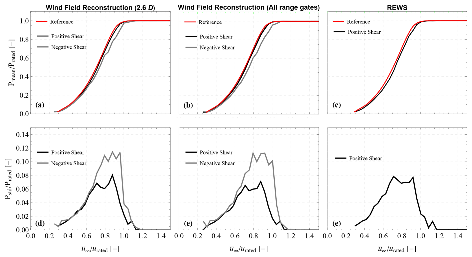
Figure 7 Normalized power produced by turbine HS4 at Hywind Scotland versus (a) the wind speed measurements from the nacelle-mounted anemometer, (b) the hub-height wind speed estimated using the nacelle-mounted wind lidar, and (c) the REWS.

To quantify the variations between the estimated power curve and the reference curve, we calculate the relative difference using three different wind speed estimates. Figure 8 shows the relative mean difference between cases with negative and positive shear, and the reference power curve for different wind speeds. The differences observed in Fig. 7 are quantified by calculating the relative percentage difference between the measured and modelled power curves. We find that when the wind profile exhibits negative shear, power production is reduced by up to 18 %. Smaller differences are observed in cases with positive shear. Interestingly, the difference between positive and negative shear ranges from 5 % to 10 %, depending on whether all range gates are used or only measurements at 2.6D are selected. The variation of the produced power is attributed to both the shear and veer values of the wind profile. In the examined dataset, negative shear values are usually related to negative veer values which results in reduction to the power production (see Appendix C). This result is in agreement with the findings reported by Murphy et al. (2020) and Paulsen et al. (2026) for the cases of onshore and offshore fixed-bottom wind turbines, respectively.

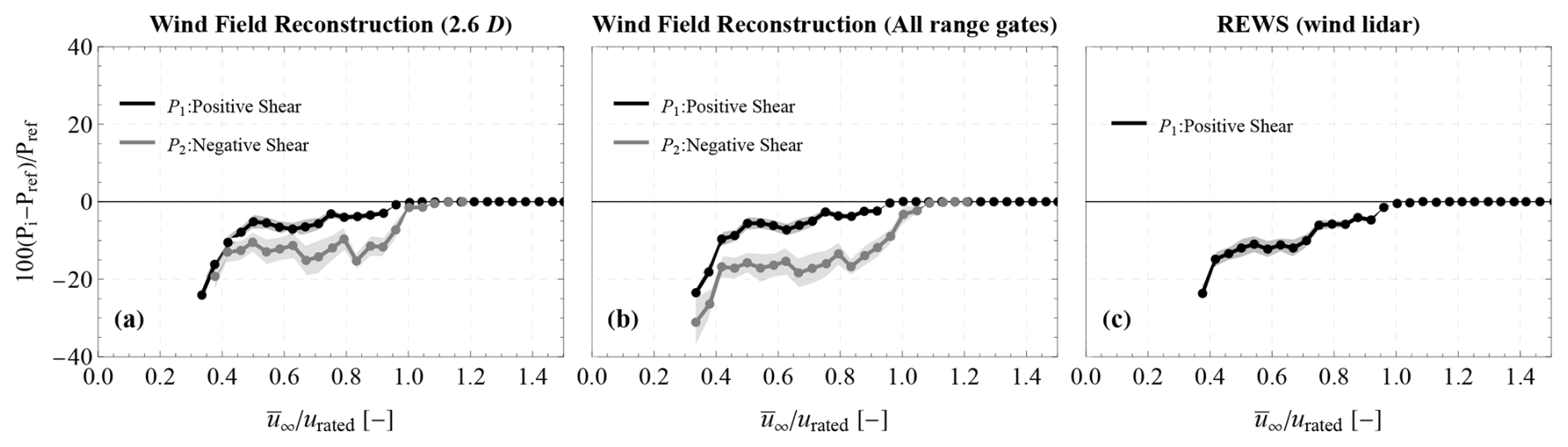
Figure 8 Relative mean difference between the estimated and the reference power curve versus the hub-height wind speed calculated using either (a) all the radial wind speed measurements or (b) only the measurements at 2.6D and (c) the REWS. In the plots (a) and (b), data from both negative and positive shears are used, while in the case of the REWS (c), only cases with positive shear are used. The shaded area denotes the 95 % confidence interval of the relative mean power differences.

5 Discussion

Two main limitations are identified in this study, which are related to sample size and available meteorological data. First, the characterization of the wind profile was based on observations acquired between June and November. Therefore, it is not possible to determine whether the derived statistical distributions of wind shear (Fig. 4) and LLJs' features (Fig. 6) are representative throughout the year or follow a specific seasonality. Similar studies that have been performed over 12-month periods report varying numbers of the frequency of LLJs over the North Sea (Kalverla et al., 2017; Rausch et al., 2022; Paulsen et al., 2026), which possibly is due to the different definitions of a LLJ (Paulsen et al., 2026). However, both Kalverla et al. (2017) and Rausch et al. (2022) report an increase of the LLJ appearance during the spring and summer seasons, which is in the same direction, with the results presented in Fig. 4 when the summer and autumn months are compared. Similar results are reported by Olsen et al. (2025). However, in our study, wind speed profiles with inversions are detected also in the case of September, which is not expected according to model predictions (Olsen et al., 2025). Second, measurements of the vertical gradient of atmospheric temperature were not available during the field campaign. Consequently, it is not possible to assess the stratification of the probed atmospheric layer, preventing classification of the data by atmospheric stability, a step that would enable a more detailed characterization of inflow wind conditions, as well as an assessment if the appearance of LLJs is related to atmospheric stable stratification (Rausch et al., 2022).

The inflow conditions are parameterized assuming a simplified vertical distribution of wind speed. Using this parameterization, we estimate hub-height wind speed for power performance verification of the wind turbine. If the turbine response is approximated as a beam, variations in the pitch and roll angles can be used to estimate the horizontal translation of the nacelle along the longitudinal and transverse axes relative to the yaw direction. Considering these variations, we find that the standard deviation of the transverse and longitudinal nacelle speeds are less than 0.2 m s⁻¹. These values introduce an uncertainty in hub-height wind speed estimation (Gräfe et al., 2023). However, due to their small magnitude, they are not considered for the case of the FOWT examined in this study. Another source of uncertainty in estimating the hub-height wind speed is the dynamic variation of the yaw direction. To minimize potential biases, only periods with a yaw direction standard deviation below 10° were considered. This threshold was chosen empirically. The resulting dataset is characterized by an average yaw direction standard deviation of 2.6°, indicating that the impact of yaw motion variability is expected to be minimal.

In our study, we find a decrease in the power curve between a FOWT and the theoretical modelled of fixed-bottom wind turbine. This difference could be partially attributed to the added tilt angle of the rotor during the operation of a FOWT. However, the observed deviations between the reference power curve and the measured one during occasions with a positive wind shear point to the direction that the offshore wind characteristics can have a significant impact on the performance of a FOWT. For example, the aerodynamic response of the FOWT and its overall power production will be impacted by the relative height of the wind speed inversion in relation to the FOWT's rotor, along with the shear and veer above and below the speed inversion (Paulsen et al., 2026). Since we do not have measurements of the wind profile at the lower part of the rotor, we cannot identify where exactly the wind speed inversion occurs in the cases of the wind profiles with negative shear. Therefore, in these cases it is not possible to provide a representative estimation of REWS, which would enable a more thorough study of the power production of the FOWT. An estimation of the REWS in the case of wind profiles with negative shear would also enable a detailed study of the increase in the standard deviation of the mean power that is observed in the range from 0.7 to 1.1 of the normalized hub-height wind speed values.

Currently, the requirements for wind turbine power verification are described in IEC 61400-12-1 (2022). However, these standards apply to turbines installed over flat or complex terrain and do not account for the impact of turbine motion on power production or on the accuracy of the hub-height wind speed. Furthermore, they do not consider cases where the wind profile deviates from the logarithmic law, which, as shown in this study, can occur frequently. Additionally, the FOWT motion induced during operation affects both the mean (Mian et al., 2024) and the dynamic (Panthi and Iungo, 2025) power variation which increase the uncertainty in power production. Therefore, a revision of the standards is necessary that takes into account the impact of the FOWT motion, as well as the impact of the wind profile characteristics on the wind field reconstruction method used by the reference wind sensor in a PCV. In such cases, it is beneficial to use multiple measurements covering both the top and bottom of the rotor, typically provided by commercial continuous-wave wind lidars, or, for pulsed wind lidars, to include more range gates. However, the latter requires incorporating line-of-sight measurements within the induction zone of the turbine into the parameterization, and thus a model of the induction factor is necessary. In this study, the induction zone was modelled using a simplified parameterization based on the induction factor and the upwind distance. Radial variations of the induction factor along the rotor were not considered. Furthermore, the application of the induction model was applied to all range gates, even if those were located outside the rotor area. Therefore, since we do not know how the dimensions of the induction zone expand with upstream distance, we cannot be sure that the wind conditions at the further measured distances (i.e. 2.08D–2.60D) were distorted by the operation of the wind turbine. Nevertheless, given the upstream distance of those range gates, the impact of this assumption on the estimation of the induction factor and the two horizontal wind components at hub height is considered negligible.

Measurements from nacelle-mounted lidars have been incorporated into standardized PCV procedures since the publication of IEC 61400-50-3 (2022). These guidelines aim to be independent of lidar technology and apply to both flat onshore and offshore sites. The recommended installation procedure for nacelle-mounted lidars includes pre-tilting the lidar's optical axis to point a height equivalent to the hub height at a distance of 2.5D in front of the rotor. However, nacelle-mounted lidars with multiple beams often lack measurements at hub height, and the estimate wind conditions at that height are a result of a wind field reconstruction method. In this study, the nacelle-mounted lidar was pre-tilted by 2.5° so that the two lower beams were nearly horizontal when the nacelle tilt was 5°. Levelled lines of sight aligned to the yaw direction are particularly useful for studying turbulence intensity in inflow conditions (Peña et al., 2017; Guo et al., 2026) and can thus provide a useful input in power curve verification. Because the horizontal lines of sight used in this study are oriented at an azimuth angle relative to the yaw direction, they do not provide a direct measurement of turbulence intensity. Nevertheless, they can still provide insight into the turbulence characteristics of the inflow (Peña et al., 2024). In our study, the standard deviation of the radial speeds of the two lower beams reveal slightly higher turbulence conditions in the wind profile cases with a positive shear (see Appendix D). Nevertheless, the observed difference is small (i.e on average around 1 %) so it is not expected that the levels of atmospheric turbulence could explain the differences in the power production between the positive and negative shear wind profile cases.

6 Conclusions

The wind profile characteristics at the North Sea over two seasons (summer and autumn) are studied using observations acquired by a nacelle-mounted wind lidar installed at the Hywind Scotland wind farm. We found that, in 88.5 % of the cases, modelling the radial speeds using a linear wind shear and veer across the rotor, along with an induction factor representing turbine operation, provided satisfactory results within the examined height range (100–200 m). The cases in which the model failed were associated with wind speed inversions occurring within the lowest 200 m of the atmosphere. Specifically, we show that floating offshore wind turbines in deep-water environments are frequently exposed to complex atmospheric conditions, including negative wind shear and wind speed inversions within the rotor-swept area. These phenomena occurred in 22 % and 11 % of the examined cases and can have a significant impact on a power curve verification procedure that is based solely on hub-height wind speed without taking into consideration the variations in the vertical wind profile. We show that using only the hub-height wind speed as a reference wind speed to power curve verification leads to a reduced turbine power production, in respect to the corresponding power curve of a fixed-bottom wind turbine, particularly under negative shear. This is demonstrated in the case of a 6 MW utility-scale floating offshore wind turbine that experiences mainly a wind-speed-dependent pitch motion during operation. We report notable differences both in the mean and the standard deviation of the produced power between cases of wind profiles with positive and negative wind shear. Our findings confirm that nacelle-mounted wind lidars are an effective tool for detecting such inflow characteristics, providing critical insights for improving power performance assessment for FOWTs.

Appendix A: Climatology: wind gradients $\partial \stackrel{\mathrm{‾}}{u}/\partial z$ and $\partial \stackrel{\mathrm{‾}}{v}/\partial z$

Figures A1 and A2 present scatter plots of the wind gradient ${\displaystyle \frac{\partial \stackrel{\mathrm{‾}}{u}}{\partial z}}$ (subfigures: a, c, and e) and ${\displaystyle \frac{\partial \stackrel{\mathrm{‾}}{v}}{\partial z}}$ (subfigures b, d, and f) versus wind direction for the months June–August and September–November, respectively. The data correspond to 10 min mean values. The wind direction corresponds to the yaw direction of the HS4 wind turbine of the Hywind Scotland wind farm. The colour of each data point corresponds to the root mean square error of Eq. (1). In the plots, we can see that all months (except November) contain measurements from all different directions spanning from 180 to 360°. Estimations of large negative shear values are usually associated with high root mean square error values (i.e. ε_u>0.2 m s⁻¹.) which correspond to cases where the observed trends in the radial wind speed measurements cannot be reproduced by the model of Eq. (1).

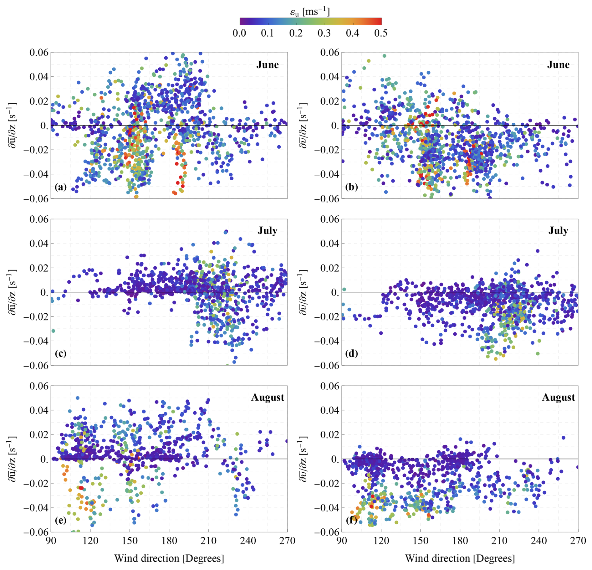
Figure A1 Wind gradients ${\displaystyle \frac{\partial \stackrel{\mathrm{‾}}{u}}{\partial z}}$ and ${\displaystyle \frac{\partial \stackrel{\mathrm{‾}}{v}}{\partial z}}$ values for different 10 min periods versus wind direction for the months June (a–b), July (c–d), and August (e–f).

Figure A2 Wind gradients ${\displaystyle \frac{\partial \stackrel{\mathrm{‾}}{u}}{\partial z}}$ and ${\displaystyle \frac{\partial \stackrel{\mathrm{‾}}{v}}{\partial z}}$ values for different 10 min periods versus wind direction for the months September (a–b), October (c–d), and November (e–f).

Appendix B: Height of the lower beams

The wind speed that is dependent on the mean pitch angle of the wind turbine nacelle results in variations in the height of the two lower beams. Figure B1a and b present the height of the two lower beams at the range gate of 2.6D. These variations have not necessarily the same magnitude in the left Fig. B1a and right Fig. B1b line-of-sight measurements due to the mean roll angle of the nacelle. The difference between the two is presented in Fig. B1c.

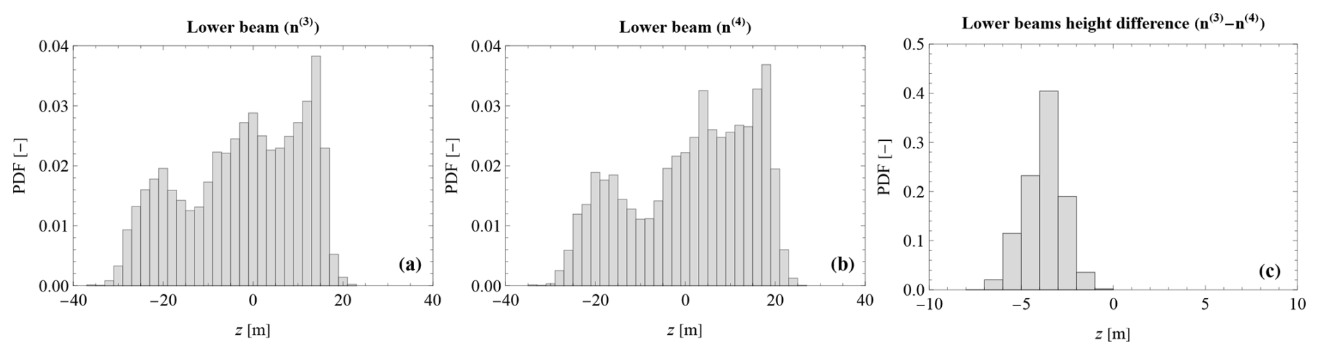
Figure B1 Probability density function of the height z of the range gate measurement of 2.6D of the left (a) and right (b) lower beams of the nacelle-mounted Doppler lidar in relation to the hub height and (c) of the difference between the two.

Appendix C: Power ratio as a function of shear and veer

Figure C1 presents the power ratio – measured power divided by the theoretical produced power using a hub-height wind speed – for different wind shear $\left({\displaystyle \frac{\partial U}{\partial z}}\right)$ and veer $\left({\displaystyle \frac{\partial \mathit{\gamma }}{\partial z}}\right)$ values estimated over 10 min periods. The estimation of the wind shear is performed by estimating the gradient of the magnitude of the horizontal wind vector between the hub height and the top of the rotor. In a similar manner, the wind veer is estimated by the gradient of the direction angle γ (defined by the inverse tangent of the two horizontal components) of the wind vector between the hub height and the top of the rotor.

Figure C1 Power ratio – measured power divided by the theoretical produced power using a hub-height wind speed – for different wind shear $\left({\displaystyle \frac{\partial U}{\partial z}}\right)$ and veer $\left({\displaystyle \frac{\partial \mathit{\gamma }}{\partial z}}\right)$ values estimated over 10 min periods.

Appendix D: Standard deviation of radial wind speed

The average standard deviation of the two lower beams using the farthest ranges of the beams is presented in Fig. D1 for the datasets that correspond to the cases with a positive (left) and negative (right) shear in the wind profile. The standard deviation values have been normalized by the mean radial speed of each beam.

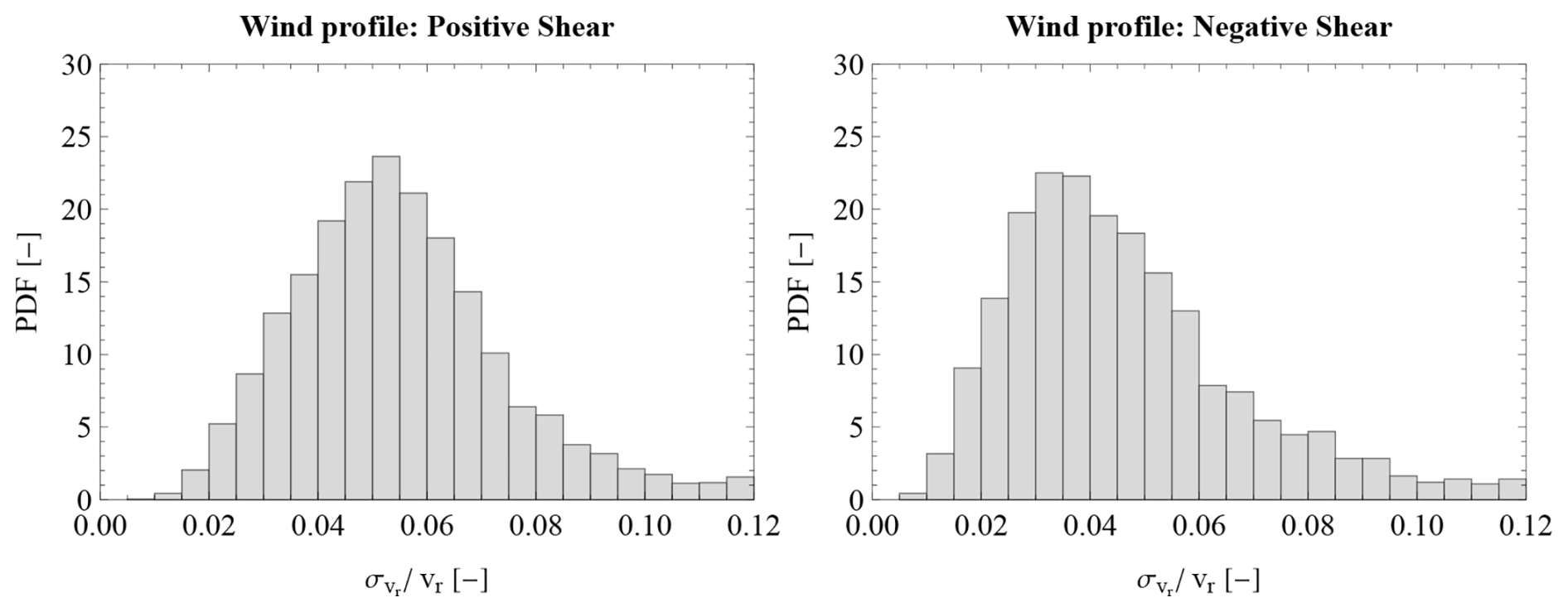
Figure D1 Probability density function of the average standard deviation of the radial speeds measured by the nacelle-mounted wind lidar at the farthest range gates and at the two lower lines of sight for the cases of wind profiles with positive (left) and negative (right) shear.