The AWAKEN wind farm benchmark – Part 1: Observed conditions

Wind turbine wakes significantly reduce downstream performance, yet accurately modeling their sensitivity to atmospheric stability and terrain remains a challenge. To address this, the International Energy Agency Wind Technology Collaboration Programme Task 57 launched a new wind farm wake benchmark leveraging high-resolution observations from the American WAKE experimeNt (AWAKEN). This paper, Part 1 of a two-part series, details the observational dataset and the selection of 24 August 2023 as the case study for the benchmark. This date was selected for its canonical diurnal cycle, which features a low-level jet with strong nocturnal stratification and high turbulence during the daytime. Analysis of the observational data reveals that despite the relatively simple terrain, interactions between the low-level jet and topography drove significant spatial variability in wind flow, leading to turbine power differences of up to 80 % across the considered wind farm. These findings demonstrate that a single vertical profile is insufficient to characterize wind plant inflow even in moderately complex terrain and that terrain-induced flow modifications can outweigh wake losses under stable stratification. The observed conditions documented here, together with the openly released dataset, constitute a unique multi-scale reference case for wake model validation at a large operating wind plant and provide the foundation for the modeling performance evaluation presented in the companion Part 2 paper.

1 Introduction

Wind turbines extract energy from the atmosphere by slowing down the wind, inevitably creating wakes – regions of reduced wind speed and elevated turbulence – downstream of individual turbines and entire wind plants (Lissaman, 1979). These wakes can extend over several kilometers (Platis et al., 2018; Abraham et al., 2024) and significantly degrade the performance of downstream turbines, reducing overall energy production and increasing structural loads (Thomsen and Sørensen, 1999; Lundquist et al., 2019).

Accurately simulating wind turbine and wind plant wakes remains a complex and open challenge. Wake behavior depends on a wide range of atmospheric and operational conditions, including atmospheric stability (Magnusson and Smedman, 1994; Iungo et al., 2013; Aitken and Lundquist, 2014; Wu et al., 2024), turbulence intensity (Barthelmie et al., 2007), wind veer and shear (Bodini et al., 2017), terrain complexity (Sun et al., 2023; Radünz et al., 2025), surface roughness (Barlas et al., 2016), and turbine operational settings (Modali et al., 2021). Stable atmospheric conditions, in particular, are known to suppress vertical mixing and allow wakes to persist over longer distances (Abkar and Porté-Agel, 2015; Barthelmie et al., 2010), while complex terrain can induce wake deflection and accelerate wake recovery (Castellani et al., 2017; Barthelmie et al., 2018; Wildmann et al., 2018). Furthermore, the coupling between mesoscale atmospheric phenomena (such as low-level jets (LLJs) or convective rolls) and turbine-scale effects is increasingly recognized as a key contributor to wake variability across time and space (Gadde and Stevens, 2021; Quint et al., 2025). As a result, modeling wake-induced losses requires resolving a wide range of scales, which presents a challenge for both standalone models and coupled frameworks (Haupt et al., 2023). Trade-offs between computational cost and physical fidelity often determine the choice of modeling approach for a given application, but no consensus yet exists on the most appropriate model type and/or the most appropriate model setup for a given model.

To address these challenges, a wide array of wake modeling approaches has been developed, each with distinct strengths and limitations depending on the target application. At the simplest level, engineering wake models – such as the Jensen/Park (Jensen, 1983; Katic et al., 1987) model – offer fast, analytical solutions based on empirical formulations of wake expansion and momentum conservation. These models are widely used in preliminary layout design and annual energy production estimates and are incorporated into industry software but often lack the ability to capture background flow and wake dynamics under realistic atmospheric or terrain conditions. More advanced empirical and semi-empirical models, including the dynamic wake meandering model (Larsen et al., 2007, 2013), introduce stochastic components or turbulence-driven dispersion to simulate wake variability and lateral movement. However, these approaches still rely on simplified inflow assumptions and may not accurately reflect interactions between multiple wakes or turbine control strategies (Andersen et al., 2014; Annoni et al., 2014).

Computational fluid dynamics models, particularly those based on Reynolds-averaged Navier–Stokes (RANS) equations coupled with actuator disk representations of wind turbines, offer greater detail by explicitly solving the governing flow equations around turbine representations (Stergiannis et al., 2016; Letizia and Iungo, 2022; van der Laan et al., 2024). While more computationally expensive, they can simulate wake interactions, shear, and terrain-induced effects with higher resolution. Still, RANS-based approaches often rely on turbulence closure assumptions and may not capture unsteady wake dynamics or mesoscale influences. At the highest (practical) level of fidelity, large-eddy simulations (LESs) resolve the largest turbulent eddies in the atmospheric boundary layer and allow for detailed, time-resolved modeling of wake behavior, including wake merging, deflection, and recovery (Jiménez et al., 2010; Wu and Porté-Agel, 2012; Churchfield et al., 2012; Vollmer et al., 2016). LES has proven invaluable in fundamental wake research and control optimization studies, but the computational cost often limits its use to research-grade, short-duration simulations.

Connecting wake modeling with numerical weather prediction and mesoscale atmospheric features, the Weather Research and Forecasting (WRF) model (Skamarock et al., 2008) has been increasingly used with embedded wind farm parameterizations to simulate wind energy impacts and wake effects over larger spatial and temporal scales. The WRF model, when coupled with schemes such as the Fitch parameterization (Fitch et al., 2012) or the explicit wake parametrization (Volker et al., 2015), incorporates turbine-induced drag and turbulence into the planetary boundary layer physics. These parameterizations treat wind farms as momentum sinks and turbulence sources, enabling the investigation of aggregated wake effects, diurnal variability, and interactions with mesoscale phenomena like LLJs or frontal systems (Arthur et al., 2020; Larsén and Fischereit, 2021; Tomaszewski and Lundquist, 2021). Although WRF-based approaches do not resolve individual turbine wakes explicitly, they are well suited for capturing farm-scale impacts and can provide valuable inflow conditions for nested LES studies (Vanderwende et al., 2016; Wise et al., 2022).

Despite the broad availability of modeling approaches, comparisons across models and configurations reveal substantial variability in predicted wake effects, even when simulating the same physical scenario (Nygaard et al., 2022). This variability stems not only from differences in model type, but also from user-defined parameters; boundary conditions; and assumptions about turbine operation, atmospheric conditions, and terrain. Moreover, model validation is often carried out using proprietary experimental datasets, which limits replicability and transparency of the results. As a consequence, wake modeling remains a significant source of uncertainty in wind plant performance assessment, long-term energy yield forecasting, and grid integration analyses (Lee and Fields, 2020; Yan et al., 2022). To address this modeling uncertainty and establish a more consistent framework for model evaluation, the International Energy Agency Wind Technology Collaboration Programme (IEA Wind) launched Wind Task 57: the Joint Assessment of Wind Energy Models. Task 57 builds on the foundations laid by IEA Wind's previous WakeBench initiative (Task 31; Sanz Rodrigo et al., 2014; Moriarty et al., 2014), which fostered an international community of researchers, industry partners, and model developers working toward standardized benchmarking of wind and wake models. WakeBench successfully created collaborative benchmarking frameworks, and Task 57 expands these efforts by incorporating new, high-resolution field measurements and advanced uncertainty quantification techniques to critically evaluate and compare state-of-the-art modeling tools.

The first benchmark under Task 57 focuses specifically on wind plant dynamics. Its aim is to systematically assess how well various modeling approaches capture wind conditions and wake features – such as momentum deficits, enhanced turbulence, and the resulting reductions in power production on downstream turbines – under realistic atmospheric and operational conditions. The benchmark design is grounded in data from the American WAKE experimeNt (AWAKEN; Moriarty et al., 2020, 2024), a large, multi-institutional field campaign designed to provide high-fidelity observations of wind plant–atmosphere interactions. These interactions are a leading source of uncertainty in both preconstruction energy yield assessments and operational forecasting. By offering a robust dataset for model validation, AWAKEN enables more rigorous benchmarking that can ultimately guide improvements in wake modeling tools and reduce uncertainty in wind energy predictions.

This paper presents an overview of AWAKEN and the relevant observations (Sect. 2), the selection of the benchmark case study and its observed meteorological and operational conditions (Sect. 3), and conclusions and lessons learned from the planning of the benchmarking exercise (Sect. 4). A companion Part 2 paper (Bodini et al., 2026) focuses on the modeling results of the benchmark.

2 The AWAKEN campaign

The AWAKEN project (Moriarty et al., 2020, 2024) is a large-scale, multi-institutional field campaign designed to observe and simulate interactions between the atmospheric boundary layer and operating wind plants. Running from October 2022 through July 2025, AWAKEN focused on a cluster of five wind plants (two of which are shown in Fig. 1) in northern Oklahoma, United States. The campaign is led by the National Laboratory of the Rockies (NLR), with contributions from numerous research institutions primarily funded by the US Department of Energy.

AWAKEN leveraged an extensive and diverse suite of instruments, including lidars (both ground-based and nacelle-mounted), X-band radars, sonic anemometers, thermodynamic profilers, and other meteorological sensors, which are deployed across 13 ground-based sites and 5 instrumented wind turbines to enable high-resolution characterization of wind plant–atmosphere interactions. Deployment timelines and observations for each instrument platform are available at https://a2e.energy.gov/project/awaken (last access: 16 July 2026) and in Moriarty et al. (2026).

2.1 Wind turbine characteristics

Turbine locations and specifications for the King Plains and Armadillo Flats wind plants were released as part of this benchmark and are available, with the rest of the data released in the benchmark, on Zenodo (Bodini et al., 2025). Table 1 summarizes key parameters for the two wind plants. Due to the proprietary nature of some of the data, the team only received approval to share benchmarking results for the King Plains wind plant, which is the focus of the results presented here and in the companion paper.

Table 1 Wind plants of interest for the AWAKEN wind plant wake benchmark.

Open-source turbine models – including thrust and power coefficient curves as well as blade aerodynamic data for each of the four turbine types in Table 1 – were provided to the benchmark participants (NLR, 2026d). Turbine models were created from the IEA 3.4-130 reference turbine through a series of numerical optimizations using the WISDEM/WEIS toolkit (NLR, 2026c). Within WISDEM/WEIS, aeroelastic simulations were run in OpenFAST (NLR, 2026b) with a ROSCO wind turbine controller (NLR, 2026a). The structural design process consists of three successive optimizations to produce a target wind turbine from an existing reference: a combined aeroelastic and structural simulation for blade, rotor, and nacelle geometry without stall constraints; a rerun of the preceding step with stall constraints; and a structural simulation for tower geometry. Once the optimized structural model was obtained, turbine performance was evaluated by first tuning the ROSCO controller parameters, then by performing a parameter sweep of wind speeds from 3–25 m s⁻¹. Each wind speed was replicated with 6 random turbulence seeds for a total of 132 simulations per turbine model. Turbine performance was logged in each simulation and averaged across turbulence seeds to produce power and thrust curves. Figure 2a shows the provided open-source power curves of the four turbine types. We emphasize that these aeroelastic simulations were not performed to predict energy production or loads for the benchmark day; measured power is directly available from the SCADA system (Sect. 2.2). Rather, their sole purpose was to generate open-source surrogate turbine models (power and thrust coefficient curves and blade aerodynamic data) that benchmark participants could implement in their wake models in place of the actual turbine specifications, which are proprietary and could not be publicly released. A comparison between the resulting open-source power curve and the SCADA-recorded power on the benchmark day is presented below (Fig. 2b).

We acknowledge that the open-source models are numerical approximations of the proprietary turbines installed at King Plains and Armadillo Flats and that some discrepancy between the open-source and true performance curves is unavoidable. A formal validation against proprietary manufacturer data is not possible given confidentiality constraints. We can, however, compare the King Plains open-source power curve against SCADA-recorded power on the benchmark day. For each King Plains turbine, the 1 min SCADA power was compared against the open-source curve as a function of density-normalized nacelle wind speed (IEC 61400-12-1, with air density measured at site A1) after removing curtailed periods and binning in 0.5 m s⁻¹ intervals. Aggregated across the minimally curtailed (<1 % curtailment) turbines, the open-source curve reproduces the production-weighted binned power with a bias of +0.1 % and an RMSE of 2.2 % of rated power (Fig. 2b), spanning the Region 2 operating range that characterized the majority of the benchmark day. Individual turbines deviate more widely, with the best-agreeing turbines distributed throughout the array. We therefore attribute this scatter to differences in the local inflow sampled by each nacelle anemometer and per-turbine calibration rather than to a systematic error in the open-source curve. The largest deviation occurs as wind speeds approach rated (above $\sim \mathrm{10}\mathrm{m}{\mathrm{s}}^{-\mathrm{1}}$), where bin-averaged SCADA power falls below the open-source curve (Fig. 2b). This behavior is expected: the open-source curve is a deterministic, steady-state relationship with a sharp transition to rated power, whereas 1 min SCADA power near the knee of the power curve reflects turbulence- and controller-induced smoothing, which systematically lowers bin-averaged power in this transition region. Moreover, relatively few 1 min samples reached near-rated wind speeds on the benchmark day, making these bins more sensitive to sampling variability. As the benchmark day was dominated by Region 2 operation, this near-rated discrepancy has a negligible impact on the benchmark analysis.

2.2 Observational network

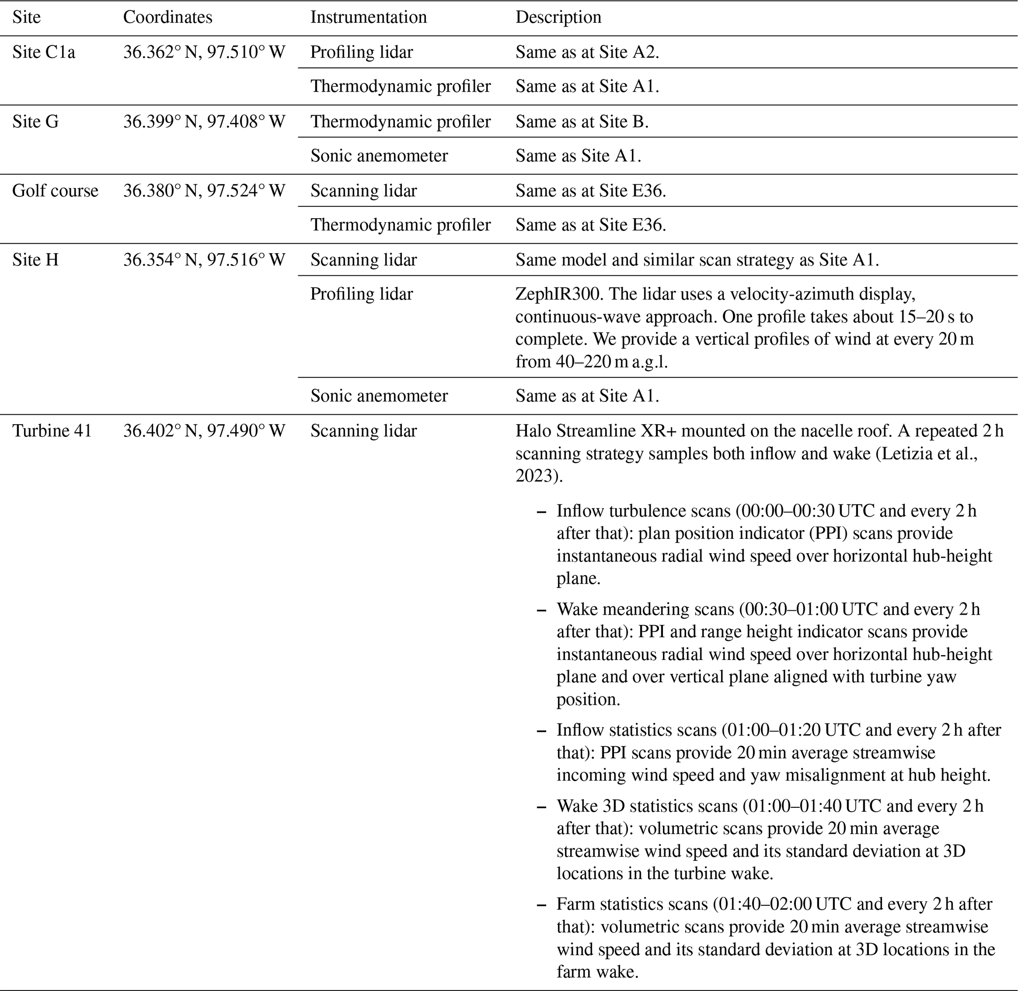
Tables 2 and 3 describe the main instruments that were deployed at the various AWAKEN upwind and downwind sites (assuming dominant winds from the south) and how they operated. Only instruments whose observations were shared as part of the benchmarking activities are included. While only a subset of these observations is directly analyzed in this paper, all listed instruments contributed data that were released to (and used by) the participating modeling teams; Tables 2 and 3 therefore serve as the reference data inventory for both this paper and the companion Part 2 paper.

Letizia et al., 2024Beck and Kühn (2017)(Turner and Löhnert, 2021)

Table 2 Instrumentation relevant to the benchmark that was deployed at the AWAKEN upwind sites.

(Letizia et al., 2023)

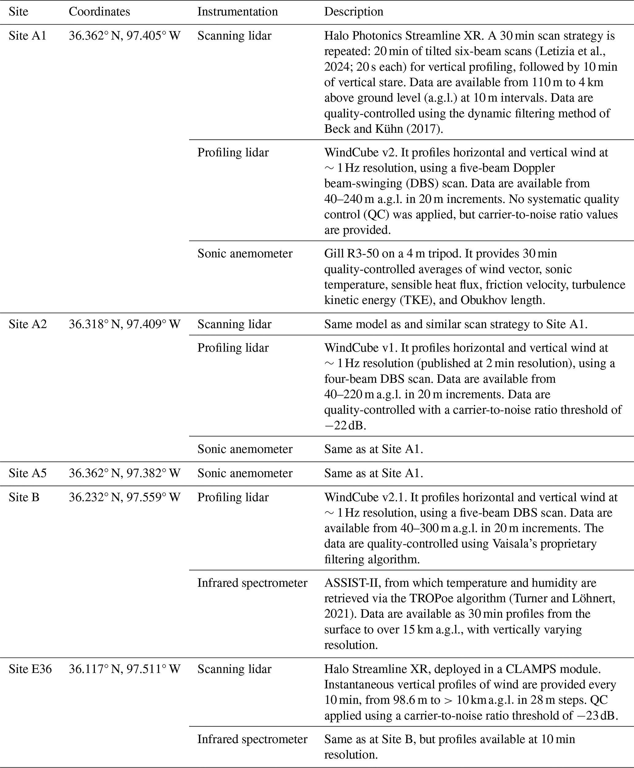
Table 3 Instrumentation relevant to the benchmark that was deployed at the AWAKEN downwind sites.

In addition to atmospheric observations, supervisory control and data acquisition (SCADA) data from all King Plains turbines are provided (for the 24 h period corresponding to the benchmark case study). The dataset, at 1 min resolution, includes turbine-level wind speed (from the nacelle anemometer), wind direction, generated power, yaw misalignment, and a binary flag indicating curtailment. Quality control (QC) was applied to the SCADA data using the OpenOA toolkit (Perr-Sauer et al., 2021) to remove erroneous sensor readings and flag curtailed operation. Normal operation was defined as having a measured wind speed between $[\mathrm{3},\mathrm{25}]\mathrm{m}{\mathrm{s}}^{-\mathrm{1}}$ and power between [1,102] % of rated power output. Periods of curtailment were identified using the relationship between power and blade pitch angle. A turbine generating a certain amount of power was considered curtailed if the blade pitch was more than 10 times the median absolute deviation from the median blade pitch at that power value.

The observational data and associated products described in this section were released to benchmark participants in three progressive phases. Phase 1 provided only a minimal upwind dataset (wind speed profiles at Site A1 up to 240 m a.g.l., surface-layer Obukhov length, and near-surface temperature), along with the open-source turbine models and farm layouts described in Sect. 2.1. In Phases 2 and 3, progressively richer inflow and wake observations were released – including additional upwind lidar sites, thermodynamic profiles, turbulence data, and ultimately the full King Plains SCADA dataset – to enable iterative model improvement. The specific variables released in each phase are summarized in Table 1 of the companion Part 2 paper (Bodini et al., 2026). Participants were provided with recommended topographic data and land-use data, but no mandatory prescription was imposed on how to process or ingest the observations, in order to faithfully replicate the range of academic and industrial modeling best practices. All benchmark input data are publicly available on Zenodo (Bodini et al., 2025).

3 Benchmark case study: selection and observed conditions

3.1 Case study selection

This benchmark centers on a case study designed to evaluate the wind turbine and wind farm wakes within and around the King Plains wind farm (Fig. 1), where the majority of the AWAKEN instrumentation was deployed. The selected case targets wind directions from the south, which are dominant in the region (Krishnamurthy et al., 2021). These conditions allow for the evaluation of both intra-farm wake effects within King Plains and inter-farm wake interactions where Armadillo Flats potentially impacts King Plains.

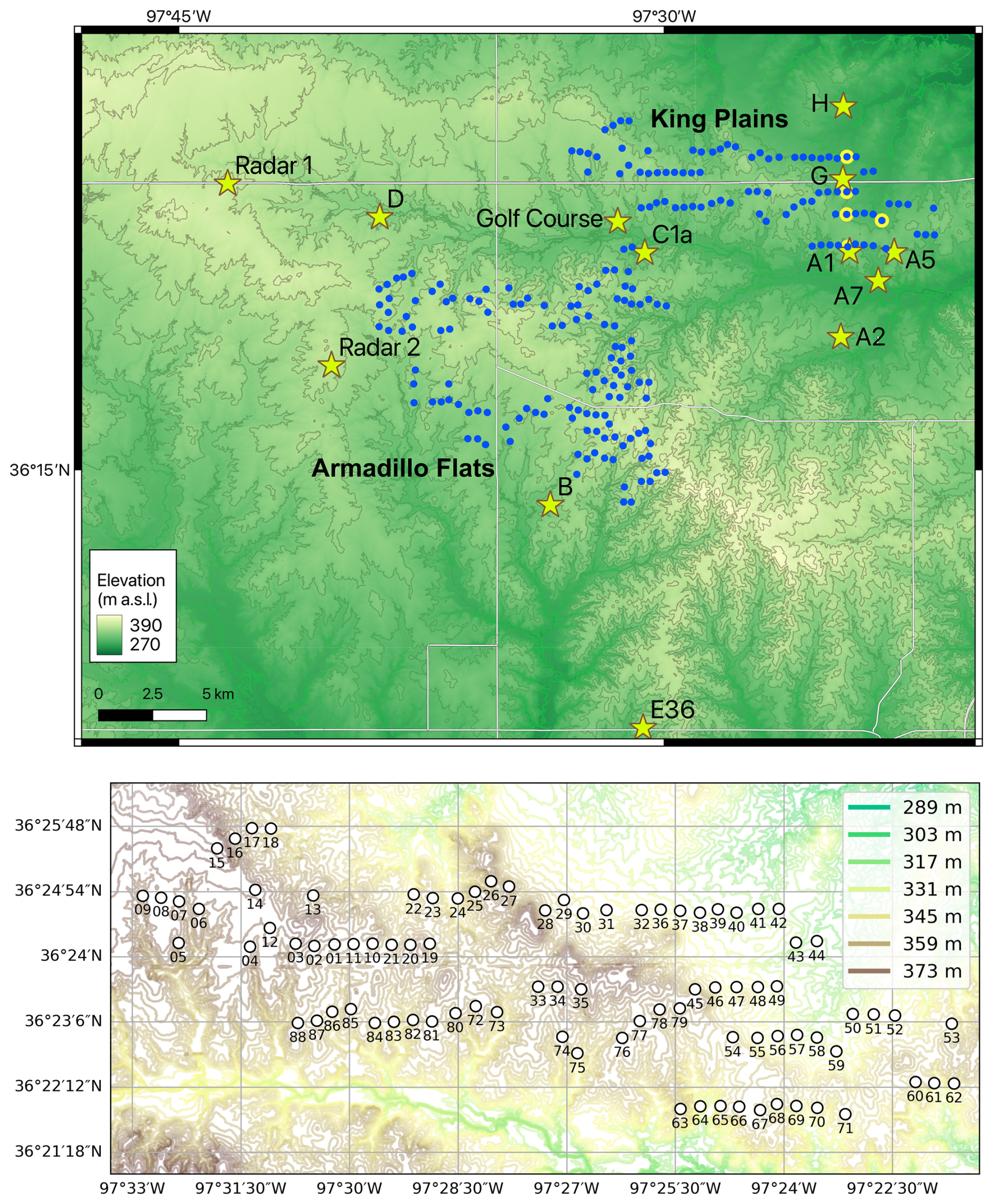
Figure 1 Top: map of the King Plains and Armadillo Flats wind plants (blue dots), instrumented sites (yellow stars), and instrumented turbines (yellow dots) in the AWAKEN campaign. The map shows 10 m terrain contours. Bottom: identification numbers of the King Plains turbines with terrain contours.

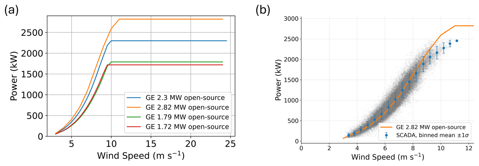
Figure 2 (a) Power curves from the open-source turbine models NLR developed for the wind turbines in the King Plains and Armadillo Flats wind plants. (b) Open-source GE 2.82 MW power curve (orange) compared against 1 min King Plains SCADA power as a function of density-normalized nacelle wind speed, aggregated across the minimally curtailed King Plains turbines on the benchmark day. Gray points are filtered 1 min observations; blue markers are bin-averaged power (±1σ) in 0.5 m s⁻¹ bins. The production-weighted bias and RMSE are +0.1 % and 2.2 % of rated power.

Given the extensive duration of the AWAKEN field campaign and the large volume of data collected, an automated search algorithm was developed to identify a 1 d reference case satisfying specific operational and observational criteria. In particular, we focused on periods when (i) more than 80 % of turbines in both the King Plains and Armadillo Flats wind farms were operating normally the whole day, (ii) nacelle-mounted lidar data from the northernmost instrumented turbine in King Plains (Turbine 41; see Fig. 1) were available, (iii) ground-based lidar data from sites A1 and H were available, and (iv) the wind direction at 90 m (measured at Site A1) ranged between 135° and 225° (dominant conditions) throughout the day. Approximately 700 h met all four criteria, but only a small number of days maintained them consistently over a complete 24 h period – a requirement essential for capturing the full diurnal cycle of wake behavior. From this reduced pool, candidate days were then assessed qualitatively against additional meteorological criteria: the absence of synoptic disturbances (e.g., frontal passages or convective activity); a clean diurnal stability cycle representative of the region (stably stratified conditions at night transitioning to a well-mixed convective boundary layer during the day); and wind speeds falling predominantly within Region 2 of the turbine power curve – in which the rotor thrust coefficient is highest, and wake deficits are therefore expected to be most pronounced. Together, these qualitative criteria ensured that the selected day would serve as a canonical reference case for studying the full range of atmospheric stability effects on wind farm wakes under conditions that are both representative of the site climatology and dynamically significant for wake evolution.

Based on these constraints, we selected 24 August 2023 as the benchmark case study. The selected day is representative of the summer southerly flow regime that dominates wind plant operation at this site. Drawing on the long-term boundary layer climatology documented by Krishnamurthy et al. (2021) for the ARM SGP Central Facility, which is situated approximately 60 km north of the AWAKEN domain and shares the same regional climate regime, several characteristics of the benchmark day fall within climatological norms. First, the nocturnal low-level jet is a persistent feature at this site, with spring and summer together accounting for approximately 60 % of LLJ occurrences. In summer, the LLJ nose is predominantly below 600 m a.g.l. (modal height $\sim \mathrm{300}-\mathrm{400}$ m) – precisely the geometry observed on 24 August 2023. Second, the strong diurnal stability cycle – stable stratification at night transitioning to a well-mixed convective boundary layer during the day – is observed over 80 % of the time at this site. Third, the southerly wind direction regime that prevailed during the benchmark day is the dominant wind direction at hub height, and summer months feature predominantly southerly flow of moderate intensity consistent with Region 2 turbine operation. Finally, the interannual variability in hub-height wind speed at the SGP site is relatively low (∼3.4 %), confirming that conditions like those of 24 August 2023 recur reliably.

Benchmark participants were tasked with simulating conditions around the King Plains (and Armadillo Flats) wind farms on this date. Participants determined their own simulated spatial extents, though we strongly recommended including both wind farms to capture inter-farm wake dynamics.

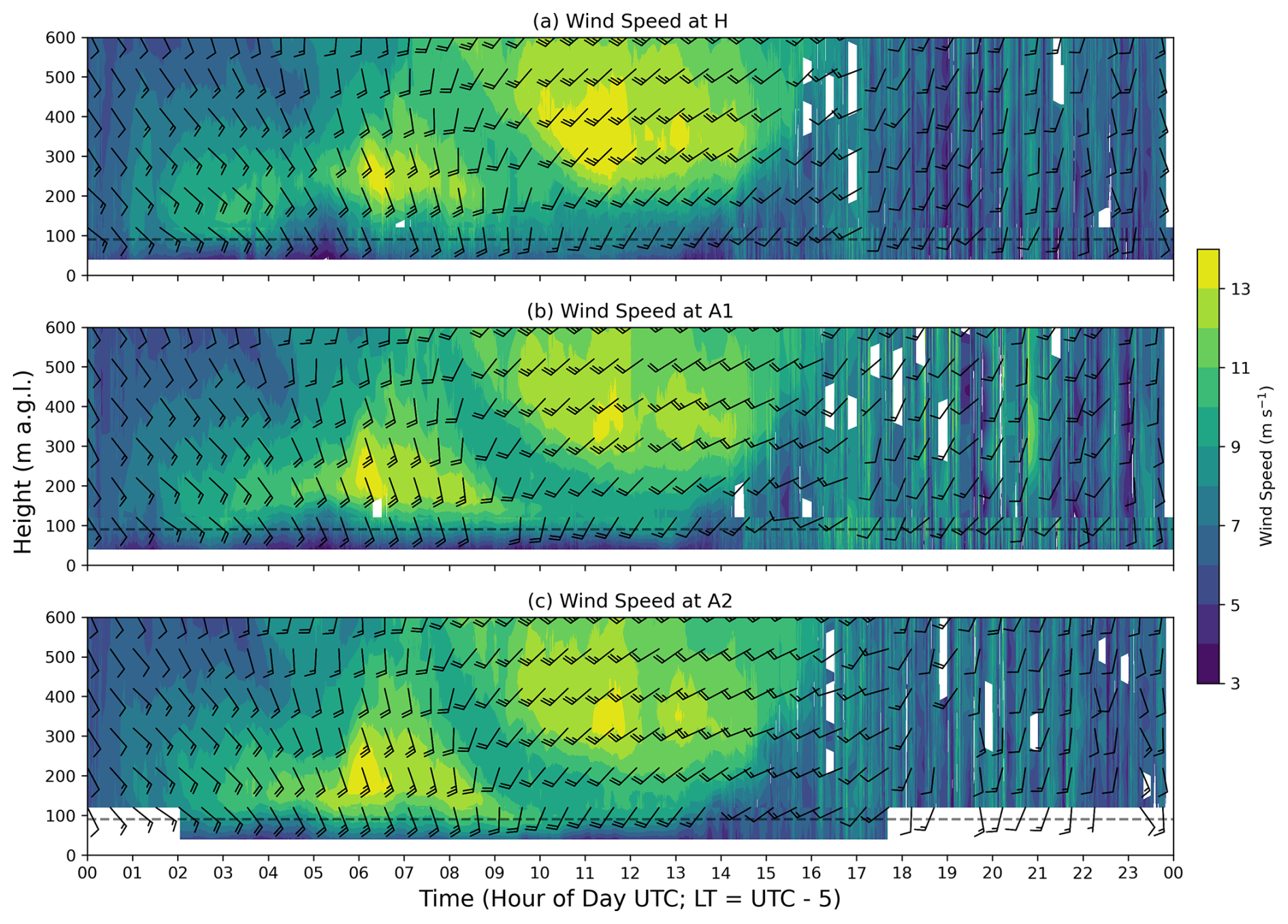
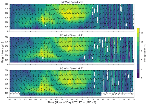
Figure 3 Time–height cross-section of observed wind speed with wind barbs to show wind direction across the AWAKEN domain on 24 August 2023 as observed from the lidars at sites (a) H, (b) A1, and (c) A2. Data from profiling lidars are shown through 120 m a.g.l., while data from the scanning lidars are used for higher altitudes. The horizontal dashed line indicates hub height (89 m a.g.l.) for the King Plains turbines.

3.2 Atmospheric inflow and low-level jet structure

Observed wind conditions on 24 August 2023 are shown in Fig. 3 (the thermodynamic observations discussed in Bodini et al., 2024, show no clouds or precipitation). A typical diurnal cycle is apparent, with low wind shear and enhanced turbulence during the local afternoon and a stably stratified boundary layer overnight. The synoptic setting on this day – characterized by a broad high-pressure ridge anchored over the southern Great Plains, weak horizontal pressure gradients over northern Oklahoma, and no proximate frontal disturbances – was particularly conducive to the development of the Great Plains nocturnal LLJ. In general, nocturnal LLJs form under quiescent synoptic conditions with clear skies, when strong nighttime radiative cooling establishes a surface-based temperature inversion that decouples the flow aloft from surface friction; the resulting force imbalance drives an inertial oscillation that accelerates the wind to supergeostrophic speeds within a few hundred meters of the ground (Blackadar, 1957). LLJs are climatologically favored over extensive plains and gently sloping terrain – where diurnal heating cycles over the slope provide an additional baroclinic forcing – as well as in some coastal regions; the US Great Plains, including the AWAKEN site, host one of the most frequent and intense LLJ climatologies in the world, with jets occurring on the majority of warm-season nights (Krishnamurthy et al., 2021). Two distinct elevated wind speed maxima are observed during the nocturnal and early-morning period. The first, occurring between approximately 04:00 and 09:00 UTC (roughly 23:00 to 04:00 local CDT), is consistent with a classic Great Plains nocturnal LLJ driven by the inertial-oscillation mechanism described above, initiated by the collapse of the daytime convective boundary layer near sunset. The jet nose of this feature descends to heights that partially intersect turbine rotor and hub levels and therefore has a direct potential impact on power production and wake structure, as discussed below. Comparing observations at the three lidar sites (A1, A2, and H), we find considerable spatial variability in the LLJ structure (Rai et al., 2026). The first LLJ is lowest at Site A2 (upwind and far from the turbines), slightly higher at Site A1 (upwind but adjacent to the southernmost King Plains turbines), and highest at Site H (downwind of the King Plains wind farm). The second wind speed maximum, observed between approximately 10:00 and 15:00 UTC (05:00 to 10:00 local CDT), is located higher in the atmosphere (approximately 400–500 m a.g.l.) and is therefore unlikely to significantly affect turbine operation directly. Its origin is less straightforward: it may reflect the slow southward progression of a weak frontal boundary evident in the synoptic analyses to the north of the site, which, as the wind direction gradually veers through the morning hours, could advect a distinct elevated residual layer or a decoupled air mass from a different source region over the area of interest. Alternatively, this feature may represent the remnant of an earlier LLJ from a different fetch that has been displaced upward as the boundary layer begins to recover after dawn. Together, the two features illustrate how complex the vertical wind structure over the site can be even on a synoptically quiescent day.

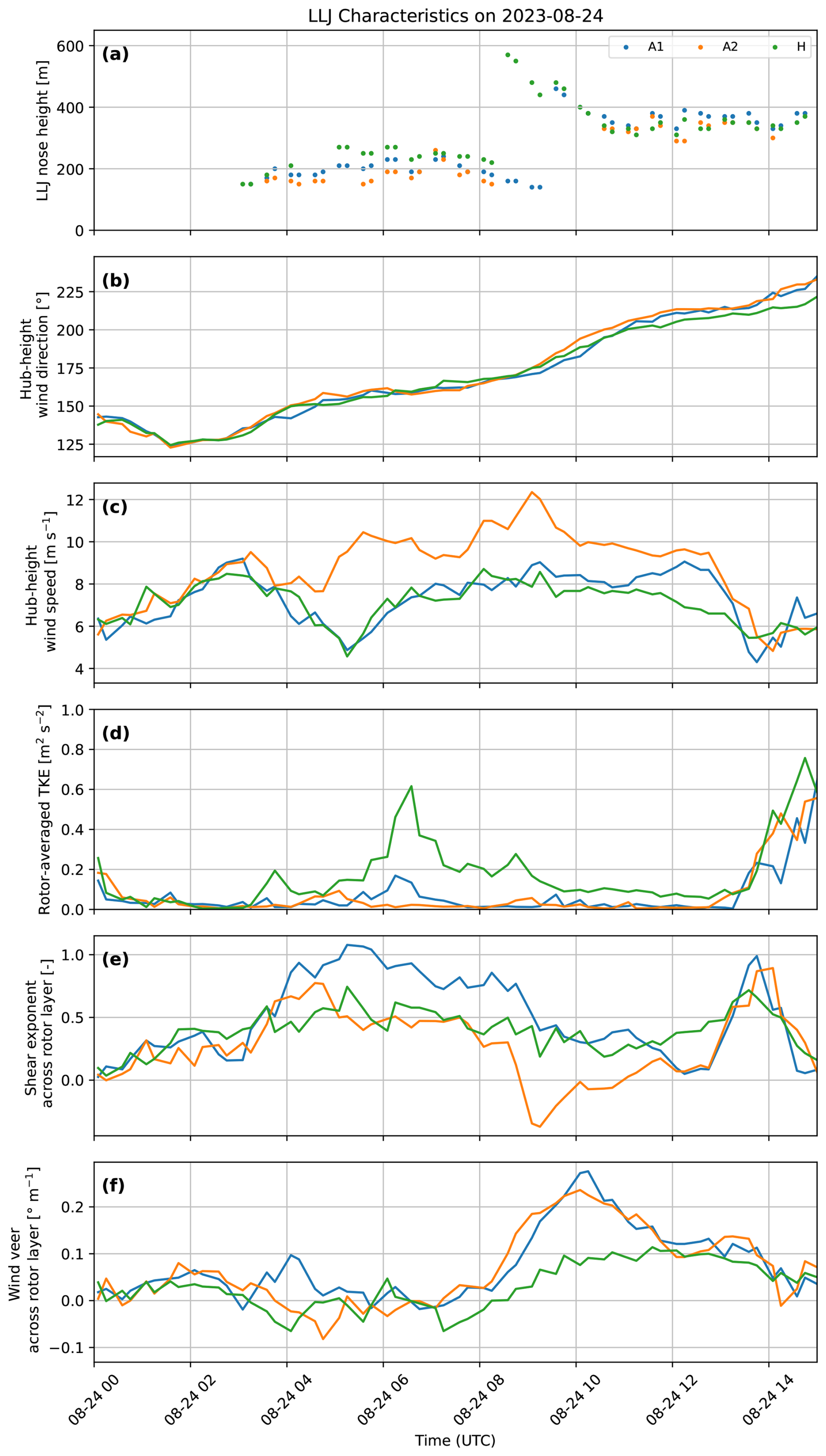
Figure 4 Time series of (a) LLJ nose height, (b) hub-height wind direction, (c) hub-height wind speed, (d) rotor-averaged lidar TKE, (e) shear exponent across the turbine rotor layer, and (f) wind veer across the turbine rotor layer at sites A1, A2, and H.

To examine this LLJ-related variability more closely, Fig. 4 shows time series of the LLJ nose height, hub-height (89 m a.g.l. for the King Plains turbines) wind speed and wind direction, rotor-averaged lidar-derived turbulence kinetic energy (TKE), and shear exponent and wind veer across the turbine rotor layer from lidars at A1, A2, and H. The shear exponent and wind veer are not computed between two discrete heights; rather, all available lidar measurement heights within the turbine rotor layer are used, with the shear exponent obtained from a power-law best fit to the wind speed profile and the wind veer from a best-fit linear rate of change in wind direction with height across the same layer. We note that the lidar-derived TKE is computed following the methodology described in Letizia et al. (2024), using a 10 min flat-detrend window consistent with wind energy industry standards, and thus includes variability across all atmospheric scales without separating turbulent from mesoscale contributions.

The first LLJ develops a nose between 140 and 300 m a.g.l. (Fig. 4a) – a range that engages the upper portion of the turbine rotor layer – and its structure is initially similar across all three sites around 03:00–04:00 UTC. Pronounced site-specific differences then emerge between 05:00 and 07:00 UTC. The key pattern in this period is a progressive lifting of the LLJ nose from the undisturbed upwind reference (A2) through the farm-adjacent site (A1) to the downwind site (H). Site A2, which lies approximately 5 km south of the southernmost King Plains turbines and is unaffected by their wakes under southerly winds, exhibits the lowest jet nose during this period – one that descends to heights partially intersecting the King Plains hub height (89 m a.g.l.) and the upper rotor layer. This alignment of the jet core with the rotor at the undisturbed inflow location represents the maximum kinetic energy available for power production. However, this resource is not fully realized at the King Plains turbines: the LLJ nose rises by roughly 100 m as the flow progresses from A2 northward over and through the wind plant to Site H. Consequently, hub-height wind speeds are highest at A2 and substantially lower at A1 and H during this period (Fig. 4c), while wind direction remains relatively constant across all three sites (Fig. 4b). The practical implication for the benchmark is direct: a model initialized solely from A2 observations that does not include the physics associated with the LLJ lifting – implicitly treating the A2 wind profile as representative of inflow conditions at the turbines – would substantially overestimate hub-height wind speeds and power production at King Plains during this period.

The cause of this localized lifting of the LLJ remains uncertain, though terrain-driven processes are a likely factor. Notably, TKE peaks sharply at Site H (and to a lesser extent at Site A1) around 06:00 UTC (Fig. 4d). A comparison of flat- and linear-detrend TKE estimates for all 10 min windows during this period (not shown) confirms that at the main TKE peak (06:20 UTC) the inflation attributable to mean-flow trends is small (∼10 % at Site H), while a single onset window (05:40 UTC) shows larger inflation (∼60 %), suggesting a partial non-stationarity contribution at the beginning of the transition.

To examine this more directly, we retrieved the vertical wind speed component w from the scanning lidar vertical stares at Sites A2, A1, and H. During the 03:00–09:00 UTC LLJ period, the stare-averaged w in the 110–200 m layer reveals a coherent spatial gradient: Site A2 (upwind) shows modest upward motion of +0.1 to $+\mathrm{0.3}\mathrm{m}{\mathrm{s}}^{-\mathrm{1}}$, Site A1 (farm edge) is near-zero, and Site H (downwind) shows persistent downward motion of −0.1 to $-\mathrm{0.3}\mathrm{m}{\mathrm{s}}^{-\mathrm{1}}$. This upwind-ascent/downwind-descent pattern, sustained throughout the 6 h window, is consistent with wave-like behavior in the stably stratified boundary layer and supports the interpretation of terrain-induced stable-layer displacement. Terrain-induced vertical displacement of the LLJ has been documented at this same site for an independent LLJ event by Radünz et al. (2025) using multiscale WRF–LES simulations, providing an independent dynamical basis for this pattern. While a hydraulic jump – as described by Peña and Santos (2021) for analogous terrain – remains another plausible mechanism, and the TKE peak at Site H around 06:00 UTC is consistent with wave breaking, the scanning lidar w observations alone cannot distinguish a hydraulic jump from broader gravity wave activity. Farm-induced flow deformation also cannot be excluded: the “deep array effect” documented by Krishnamurthy et al. (2025); Rai et al. (2026) could contribute to the observed upward motion at A2. Regardless of the precise mechanism – be it terrain-induced, wake-induced, or a combination of both – these observations demonstrate that initializing a numerical model with wind speed data from Site A2 only would lead to a large overestimation of power generation for the King Plains wind plant. Despite the relatively simple terrain in this region, significant wind speed differences arise from local interactions between the LLJ, topography, and the wind turbines themselves.

3.3 Turbine power production and spatial variability

These spatial and temporal variations in wind conditions translate directly into variability in turbine power production, as recorded by the King Plains SCADA system. Most turbines from the two wind plants were operating normally on 24 August 2023, with no significant drop in availability outside of some high-frequency fluctuations. However, Fig. 5 reveals substantial temporal variability in turbine-level power, particularly during stable nighttime conditions. A pronounced drop in power occurs around 05:30 UTC, coinciding with the local lifting of the LLJ identified in Figs. 3 and 4. Spatial heterogeneity is also evident: turbines in different locations across the farm exhibit power output differences of up to 80 % at a given time during the night (e.g., around 09:00 UTC).

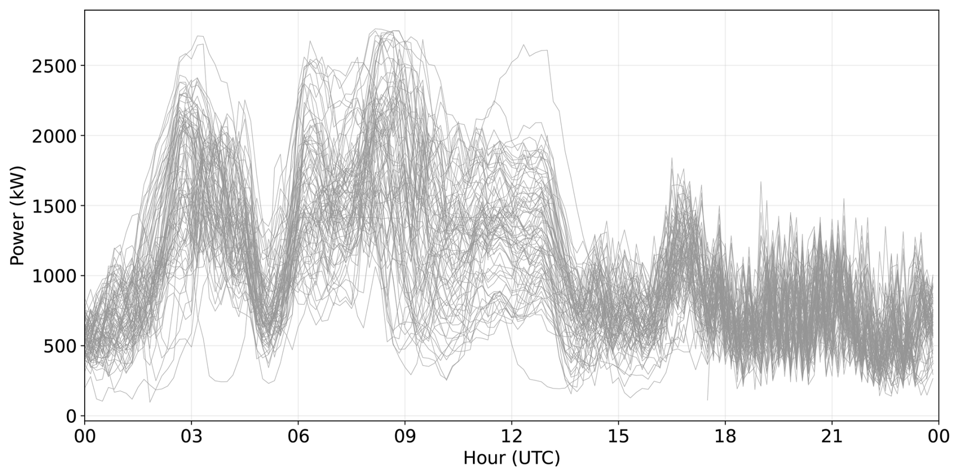
Figure 5 Time series showing the power production by each King Plains turbine on 24 August 2023.

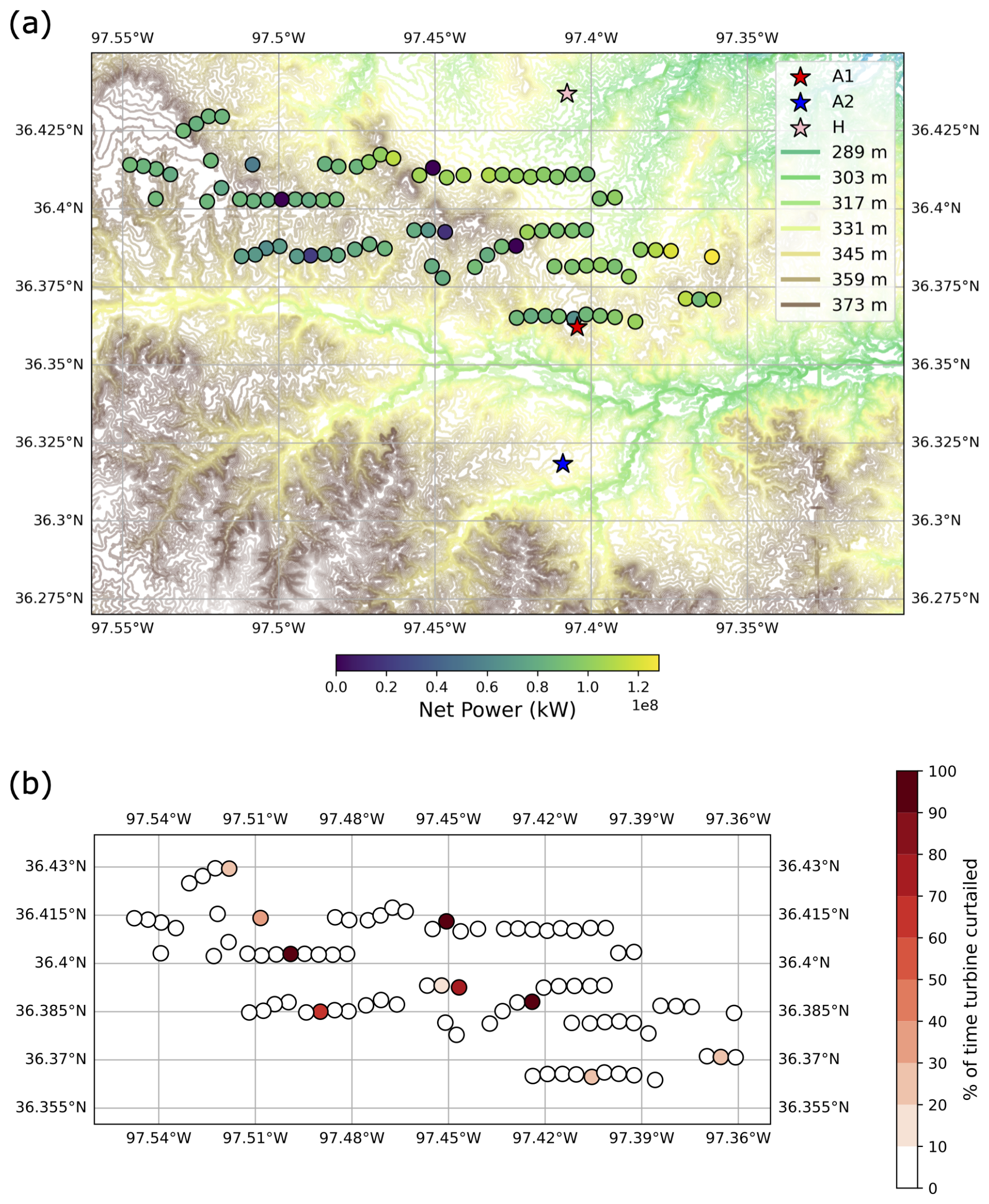
Figure 6 (a) Map of the total energy production by the King Plains turbines on 24 August 2023. (b) Map showing the percentage of time each turbine at the King Plains wind farm experienced curtailment during the benchmark day. Turbine identification numbers are provided in the bottom panel of Fig. 1.

The spatial variability in power production can be further explored by looking at a map of total energy production by each King Plains turbine on the benchmark day (Fig. 6a). Turbines in the northern and eastern portions of the farm produce more energy overall. The east–west gradient may be expected given the prevailing south-southwesterly winds and potential farm-to-farm wake effects from the upwind Armadillo Flats wind farm. However, the north–south gradient is less intuitive: northern turbines, which should be more impacted by internal wakes, still produce more energy, perhaps similar to the case study of Radünz et al. (2025). Interestingly, Turbine 53 in the eastern portion of the wind plant shows the highest energy output, likely due to local terrain-induced speedups. As the empirical orthogonal function (EOF) analysis presented below quantifies, large-scale wind speed variability – modulated by terrain – exerts a much stronger influence on turbine-level production than internal wake effects, helping to explain why the expected internal-wake signature does not dominate the north–south pattern. Before examining the spatial patterns of power variability further, it is worth noting that turbines 11, 29, and 79 were offline for the entire benchmark day (Fig. 6b); all other turbines experienced only intermittent curtailment (defined as the proportion of curtailed time stamps relative to normal operating time stamps for the benchmark day).

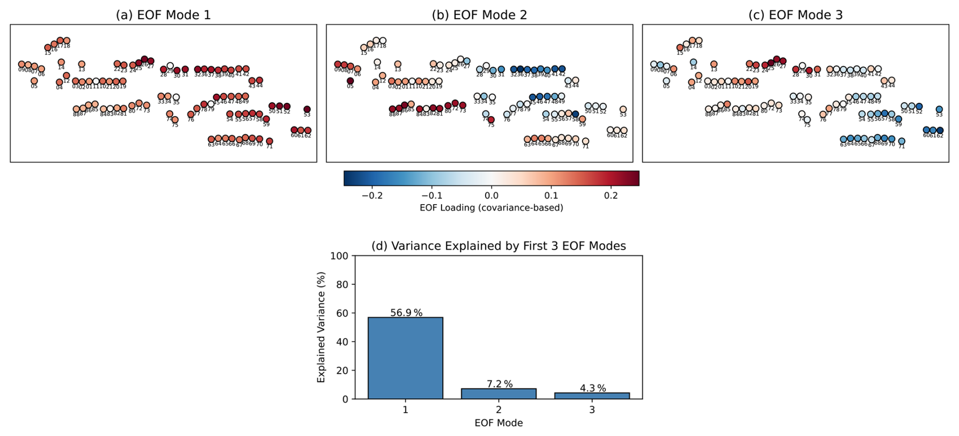
Figure 7 (a–c) Spatial variability in energy production by King Plains turbines expressed by the first three EOF modes: (a) Mode 1 captures coherent, farm-wide fluctuations driven by large-scale wind speed variability, modulated by terrain and inter-farm wake exposure; (b) Mode 2 captures the east–west contrast associated with the combined influence of inter-farm wakes from Armadillo Flats and terrain-induced speedups; (c) Mode 3 isolates internal wake variability, with reduced loadings in downstream turbines. (d) Variance explained by the first three EOF modes.

The main patterns of spatial variability in energy production are systematically assessed by computing EOFs of turbine-level power production across the King Plains wind farm for the benchmark day (Fig. 7a–c). The EOF analysis was applied to the power output from all 88 King Plains turbines recorded by the SCADA system over the full 24 h benchmark day. To reduce high-frequency turbulent noise and focus on physically meaningful timescales, the 1 Hz SCADA data were first resampled to 1 min averages, yielding 1440 temporal snapshots. Each turbine time series was mean-centered by subtracting its 24 h mean; unlike a correlation-based approach, the time series were not normalized to unit variance. This covariance-based formulation preserves the physical magnitude of power fluctuations: turbines with higher intrinsic variance contribute to the decomposition in proportion to their actual variability, rather than being artificially equalized with chronically wake-affected or curtailed turbines whose power fluctuations are structurally suppressed. Turbines that were offline for the entire benchmark day produce a zero-mean-centered time series and are therefore excluded from the variance pool, appearing as zero loadings in Fig. 7. The decomposition was performed via singular value decomposition. EOF signs are arbitrary, but relative phase differences between turbines are preserved to maintain physical interpretability. The first mode (56.9 % of total variance) captures coherent, farm-wide fluctuations in production driven by large-scale wind speed variability, as confirmed by the corresponding principal component time series (not shown), which closely tracks the diurnal wind speed evolution. The non-uniform loading pattern in Mode 1 reflects how terrain and inter-farm wake exposure modulate each turbine's absolute power variance. Turbines in the northeastern sector – where terrain-induced speedups produce persistently elevated power output – carry the largest loadings, while turbines in the southwestern sector, intermittently shadowed by Armadillo Flats under the prevailing SSW flow, show reduced variance and thus lower loadings. Mode 2 (7.2 % of variance) captures the dominant east–west spatial contrast in time-varying production, which we attribute to the combined and largely inseparable influence of inter-farm wakes and terrain. Under the prevailing SSW flow, Armadillo Flats casts a wake shadow over the western sector of King Plains, reducing power in those turbines; simultaneously, turbines in the eastern sector benefit from terrain-induced wind speed enhancements. The third mode (4.3 % of variance) isolates patterns of internal wake variability, with consistently reduced loadings in downstream turbines. Together, the first three modes explain approximately 68 % of the total variance (Fig. 7d), highlighting the substantial complexity and heterogeneity of turbine-level power production even on a single canonical day.

To further confirm how terrain influences the spatial variability in power production, we calculated a relative elevation metric for each turbine. For every stability class (determined using the 30 min average Obukhov length, L, calculated from sonic anemometer measurements collected at Site A1; stable: L>0 m; unstable: L<0 m), we defined an upstream sector centered on the mean hub-height wind direction (from the profiling lidar at Site A1). This sector was defined by a 1 km radius and a 45° arc. We then calculated the mean terrain elevation within this upstream sector (${\stackrel{\mathrm{‾}}{z}}_{\text{upstream}}$) and subtracted it from the specific turbine's base elevation (z_turbine):

$$\begin{array}{}\text{(1)}& \mathrm{\Delta }{z}_{\text{rel}}=z_{\text{turbine}}-{\stackrel{\mathrm{‾}}{z}}_{\text{upstream}}.\end{array}$$

This Δz_rel value, expressed in meters of elevation difference and derived from the United States Geological Survey $\mathrm{1}/\mathrm{3}$ arc-second (approximately 10 m horizontal resolution) digital elevation model, represents the turbine's elevation relative to the mean terrain it “sees” immediately upwind. A positive value indicates the turbine is situated higher than the upstream fetch (e.g., a ridge, hilltop, or positive slope) relative to the incoming flow, while a negative value indicates a local depression or negative slope. By calculating this for each stability class, we account for the fact that the “effective” upwind terrain changes as the mean wind direction shifts with atmospheric stability. Figure 8 shows turbine power output as a function of this upwind elevation difference for stable and unstable conditions. In both cases, turbines situated lower than the upwind terrain (left side of the plots) tend to produce more power, especially under stable conditions, despite being located downwind of other turbines in the King Plains case. This counterintuitive result aligns with numerical findings from Radünz et al. (2025), who suggested that terrain-induced acceleration of hub-height winds can outweigh the effects of turbine wakes at the AWAKEN site, particularly under stably stratified conditions. These results suggest that models relying solely on flat-terrain assumptions or standard wake decay curves without terrain corrections will likely misinterpret the performance drivers on this day.

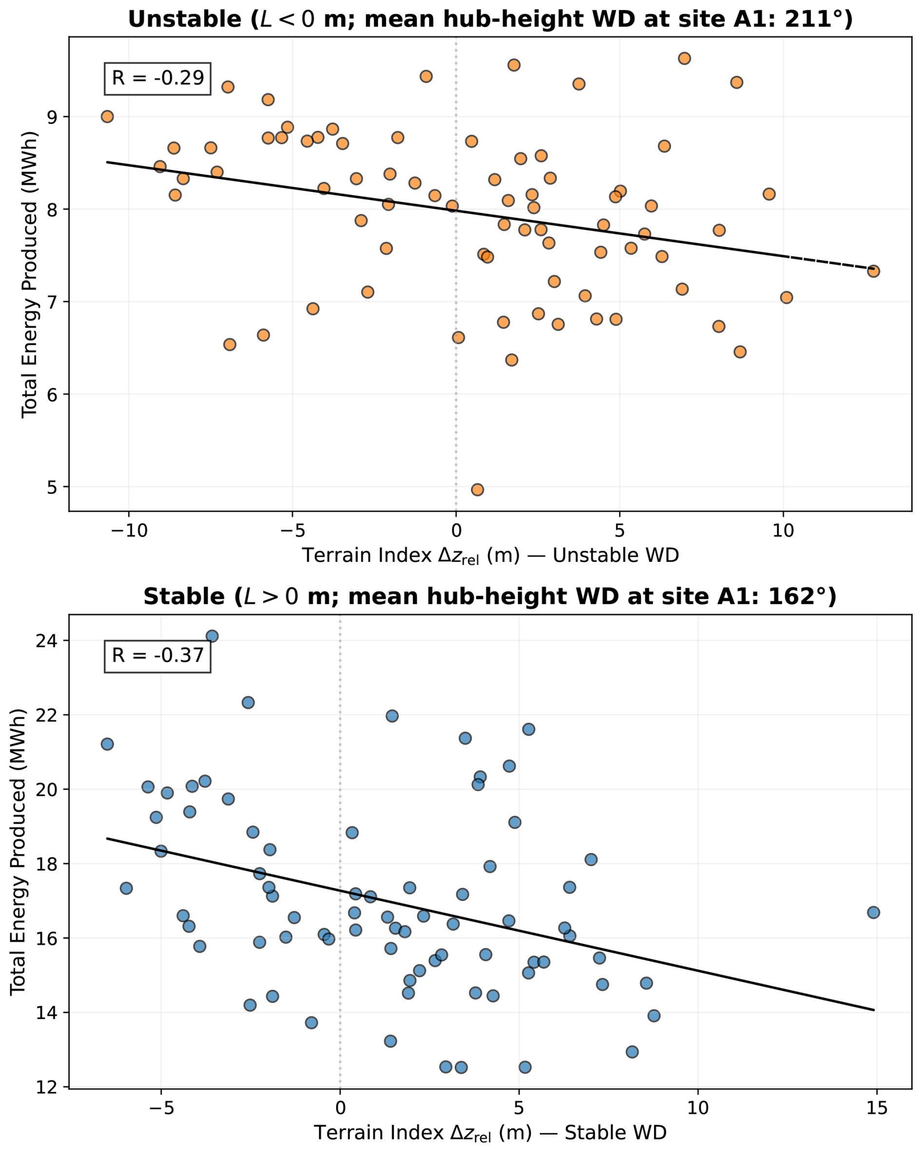
Figure 8 Total energy produced by King Plains turbines as a function of upwind (45° sector aligned with the mean hub-height wind direction (WD) measured at Site A1 for each stability class) terrain variability for (top) unstable and (bottom) stable conditions on 24 August 2023. Turbines that experienced curtailment are not included.

3.4 Observed wake characteristics

While terrain-related effects might make wake signatures murkier, the comprehensive AWAKEN measurements still allow for their assessment and characterization. As detailed in Bodini et al. (2024), the suite of scanning and profiling lidars – deployed on the ground, on turbine nacelles, and on a mobile platform – captured the wind plant wake dynamics at King Plains during the selected case study. A clear wake-induced wind speed deficit of over 1 m s⁻¹ was observed at Site H, located 22 rotor diameters downwind of King Plains, particularly above the turbine hub height (Fig. 9). These wake impacts were most evident during nighttime stable conditions, when low turbulent mixing delayed wake recovery, and the LLJ was lifted. In contrast, under daytime unstable conditions, enhanced turbulence eroded the wakes almost entirely before reaching Site H. Additionally, nacelle-mounted lidars on the northernmost row of King Plains turbines revealed the spatiotemporal evolution of single-turbine wake structures and their dependence on atmospheric stability.

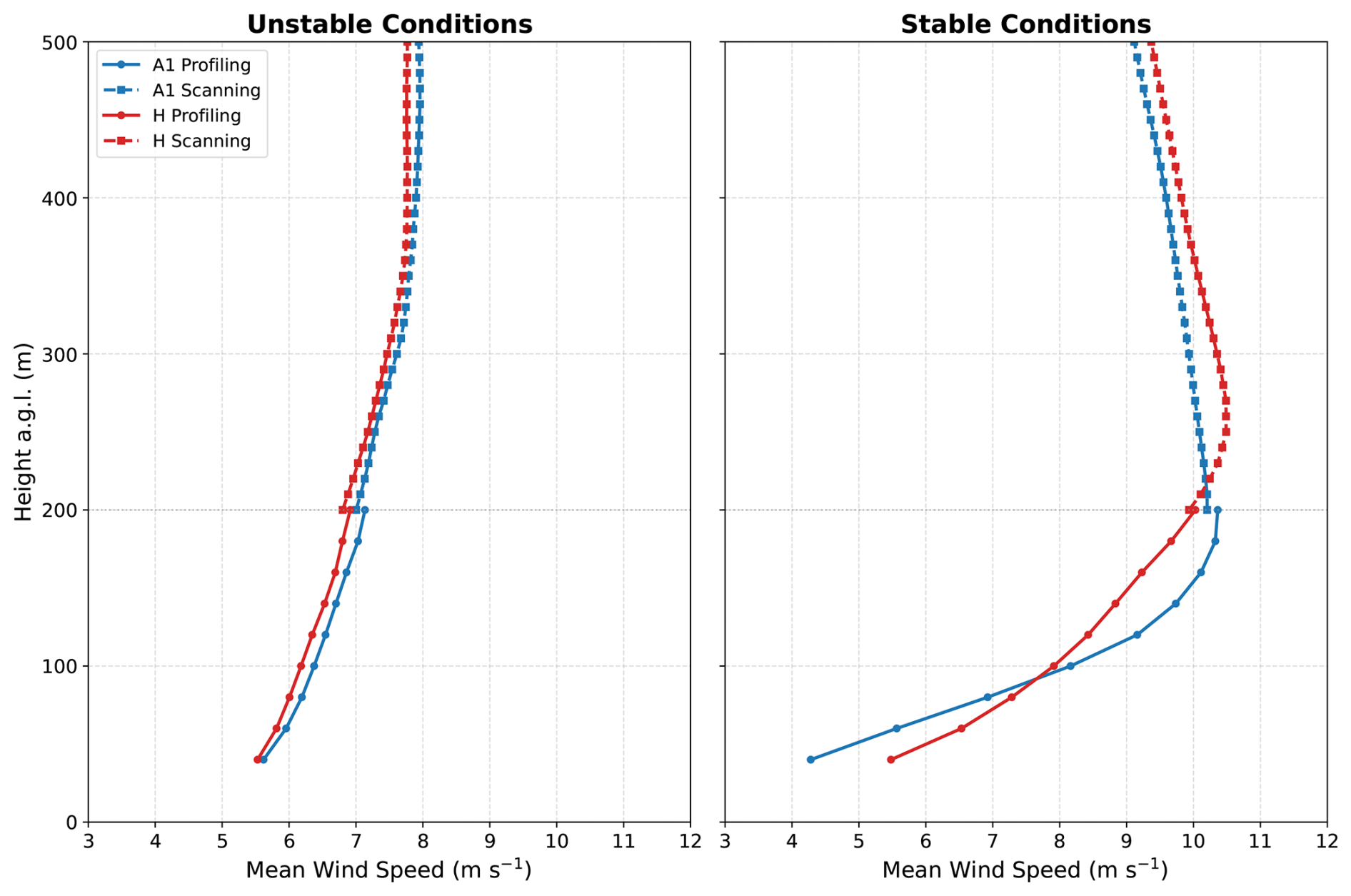
Figure 9 Mean vertical profiles of wind speed at sites A1 (blue) and H (red) during unstable (left) and stable (right) atmospheric conditions on the benchmark day. Profiles are constructed using a composite of profiling lidar data for the rotor layer (z≤200 m; solid lines) and scanning lidar data for the upper boundary layer (z≥200 m; dashed lines); the discontinuity at 200 m reflects measurement uncertainty at the instrument hand-off height (different sampling volumes and averaging periods) and does not correspond to a physical flow feature.

4 Conclusions

This paper introduces the design and observational foundation of the IEA Wind Task 57 wind plant wake benchmark. Leveraging the unprecedented multi-platform measurements from the AWAKEN campaign, the benchmark provides a rigorously curated case study – 24 August 2023 – selected through an automated search process to ensure high data availability, consistent turbine operations, and meteorological conditions representative of the summer southerly flow, nocturnal-LLJ regime that characterizes wind plant operation at this site (Krishnamurthy et al., 2021).

The analysis of the selected case study highlights the critical importance of resolving wind flow features across scales. Observations on 24 August 2023 revealed that a single vertical profile is insufficient to characterize inflow even in moderately complex terrain. We observed a localized lifting of the LLJ nose by approximately 100 m between sites across the AWAKEN domain, which correlated with significant power drops. Furthermore, a counterintuitive correlation between lower terrain elevation and higher power output was observed under stable conditions, suggesting terrain-induced speedups outweigh wake losses in specific stability regimes.

With the development of this benchmark, the goal was to create a controlled, transparent, and scientifically valuable framework that enables the wind energy modeling community to evaluate and improve wake modeling approaches. Several key lessons emerged from the process of organizing this benchmark. Sufficient time must be allocated for data QC and analysis before launching a benchmark, as these are critical to building trust in the dataset used to validate numerical models. Moreover, as is typical in large, multi-instrument field campaigns, full and simultaneous data availability across all platforms cannot be guaranteed. Recognizing these practical limitations is essential, and thoughtful compromises are often required. The modeling results and analysis from all three phases of the benchmark are presented in the companion Part 2 journal article.