The AWAKEN wind farm benchmark – Part 2: Modeling results

Accurately modeling wind farm performance in complex atmospheric flows remains a challenge. This paper presents the modeling results of the American WAKE experimeNt (AWAKEN) wind farm benchmark, a collaborative effort involving 16 research groups from academia and industry within the International Energy Agency Wind Technology Collaboration Programme Task 57. The study evaluates a diverse suite of simulation tools, ranging from fast-running engineering wake models to high-fidelity large-eddy simulations, against a diurnal case study observed during the AWAKEN campaign. The benchmark utilized a three-phase structure to progressively assess model performance as observational data availability increased. Initial blind predictions showed that higher-fidelity models did not uniformly outperform simpler simulation tools in terms of aggregate error metrics; however, this largely reflects differences in inflow strategy rather than wake physics fidelity – simpler models directly ingested high-quality observations, while higher-fidelity models were tasked with predicting the inflow from coarser reanalysis boundary conditions. A distinct spatial bias was observed where models struggled to resolve the interplay between a low-level jet, wakes, and terrain-induced flow acceleration. In subsequent phases, access to progressively richer observational data enabled model refinement that reduced mean absolute error by up to 40 %; however, these gains primarily reflect state-conditioned calibration to a well-observed atmospheric state. Overall, the study demonstrates that inflow characterization defines a lower bound on achievable model accuracy that is independent of wake modeling fidelity – a finding with direct implications for pre-construction energy assessment workflows. While the limited ability to resolve local terrain-flow interactions under single-day conditions represents a recognized constraint, the findings on wake modeling and real-world validation still provide valuable guidance for model application and future benchmark design.

1 Introduction

Building on the characterization of the atmospheric and operational conditions presented in the companion Part 1 paper (Bodini et al., 2026), here we focus on the modeling component of the American WAKE experimeNt (AWAKEN) wind farm benchmark, which represents the first benchmarking exercise within the International Energy Agency (IEA) Wind Technology Collaboration Programme Task 57. The benchmark brings together a diverse set of modeling approaches, from engineering wake models to mesoscale–microscale coupled frameworks and large-eddy simulation (LES), to evaluate how well current tools reproduce the observed wind flow, wake behavior, and turbine impacts documented during the selected case study.

The complexity of this task is underscored by recent benchmarking efforts that have sought to quantify model uncertainty and bias across different scales. At the single-turbine scale, results from the SWiFT site (Doubrawa et al., 2020) demonstrated that while model performance generally tracks with fidelity in neutral conditions, steady-state Reynolds-averaged Navier–Stokes (RANS) simulations can outperform higher-fidelity tools in stable conditions due to the ease of prescribing non-canonical inflows. On a larger scale, an evaluation of 19 offshore wind farms (Nygaard et al., 2022) established a wake model uncertainty of less than 10 % for models accounting for global blockage and heterogeneous flow. However, that study also revealed systematic limitations in traditional engineering tools: the standard Park model (Jensen, 1983) tends to underestimate wake losses and overestimate wind speed recovery as turbine spacing increases. While newer models like TurbOPark (Pedersen et al., 2022) have shown lower bias across varying spacings offshore, their applicability to complex land-based environments – where time-dependent turbulence and diurnal cycles dominate – remains largely untested.

Comparing models across such a broad spectrum of fidelity and complexity thus presents unique challenges. Beyond the physical representation of atmospheric stability and turbine parameterization, the “human factor” – subjective decisions made by modelers regarding grid setup, spin-up times, and mesh refinement – adds a significant layer of uncertainty. To disentangle these factors, this benchmark adopts a multiphase blind approach. By progressively releasing observational data (Sect. 2), we track not only the baseline performance of state-of-the-art tools but also their ability to adapt and improve via model calibration. Section 3 details the diverse participating models and their setup evolution through the phases. Section 4 presents the comparative results, analyzing bias, error spatial distribution, and wake-specific metrics. Finally, Sect. 5 summarizes the scientific and operational lessons learned from this extensive international exercise.

2 Structure of the benchmark

This benchmark was designed to evaluate how well different modeling approaches capture key aspects of wind farm behavior under real-world conditions, a key goal of IEA Task 57. These include the representation of inflow characteristics, wake behavior at both the turbine and farm scales, impacts on downstream farms, and, ultimately, power production. To encourage broad participation and comparison, the benchmark welcomed a wide range of simulation tools, from mesoscale models with varying parameterizations to analytical and engineering models and higher-fidelity approaches such as LES and RANS models.

We structured the benchmark into three phases, as follows.

• Phase 1: the baseline. The purpose of this phase was to replicate industry practice, where an analyst must estimate energy production based on limited observations at a site. The benchmark team released limited inflow observations for 24 August 2023 (and the previous day, in case they were needed to initialize simulations), along with the National Laboratory of the Rockies' open-source wind turbine models (described in Bodini et al., 2026) and the coordinates and dimensions of the King Plains and Armadillo Flats turbines. Participants used these inputs, combined with their own best practices, to simulate the wind flow around the King Plains and Armadillo Flats wind farms on 24 August 2023. Phase 1 officially started on 28 May 2024 and participants submitted their simulated data by 1 September 2024.

• Phase 2: model improvement with inflow observations. The team released all inflow observations and some limited supervisory control and data acquisition (SCADA) data to participants. Leveraging the additional inflow observations and insights gained from Phase 1 results, participants tried to improve their simulation results. Phase 2 officially started on 12 November 2024, coinciding with the release of Phase 1 results. Participants submitted their Phase 2 results by 15 January 2025.

• Phase 3: model improvement with inflow and wake observations. The team released all inflow and wake observations as well as all King Plains SCADA data for the selected case study. Participants used this full dataset, along with lessons learned from the first two phases, to further improve their simulations. Phase 3 officially started on 13 March 2025, with the release of Phase 2 results. Participants submitted results by 30 April 2025.

Table 1 summarizes the data released to benchmark participants during each phase, while Fig. 1 provides a schematic of the primary observational sites around King Plains (a more comprehensive map is provided in Part 1 (Bodini et al., 2026)).

Table 1 Data released to the benchmark participants in each of the three phases of the exercise.

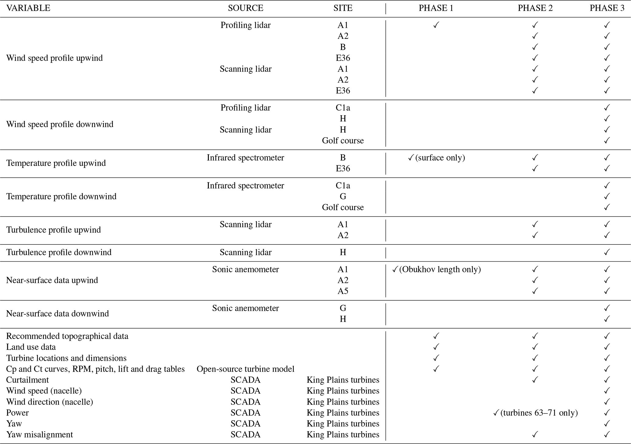
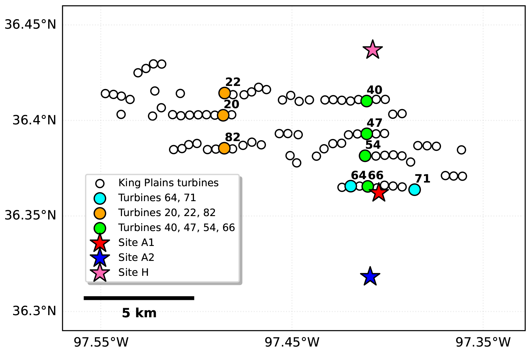
Figure 1 Map showing the King Plains turbines and the locations of sites A1, A2, and H. Highlighted turbines are those selected for detailed analyses in this paper.

3 Benchmark participants

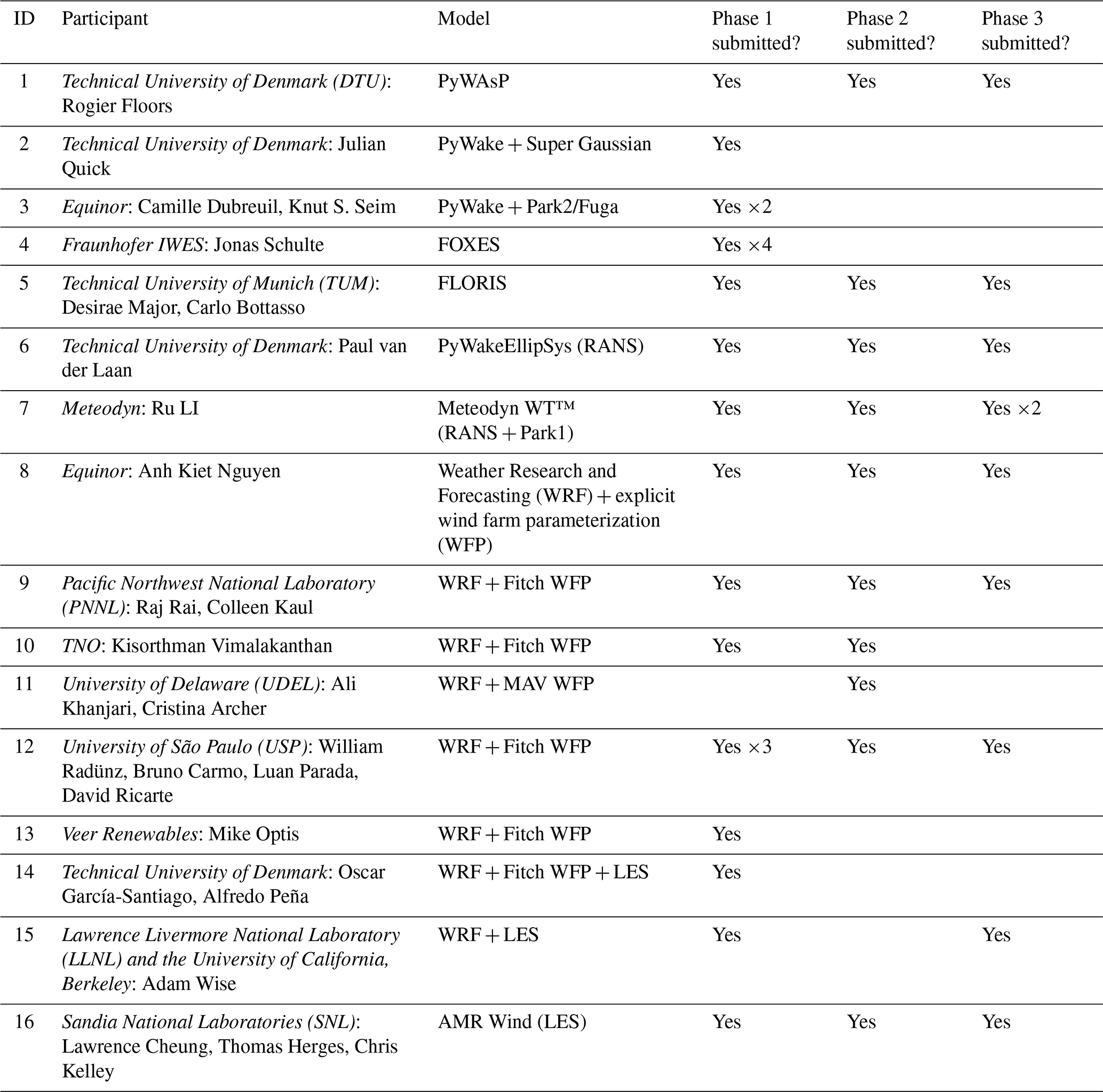
Universities, research institutes, and private companies (Table 2) from the United States, Denmark, Brazil, Germany, Canada, France, United Kingdom, Netherlands, and Norway participated in the AWAKEN benchmark. We highlight the main characteristics of the models used by each participant as well as any changes made in the model setup for those who submitted results in multiple phases of the benchmark. We also note that a few other groups participated in the benchmark but did not give us permission to publish their results. It is important to note that the ensemble presented here represents a collection of plausible model configurations reflecting participant best practices rather than a fully controlled experiment.

Table 2 Participants and submission status by benchmark phase.

3.1 Participant 1: PyWAsP by Technical University of Denmark

The wind farm flow was simulated using WAsP, a steady-state model relying on the geostrophic drag law and logarithmic wind profiles (Troen and Petersen, 1989). The wind climate input was derived from lidar observations at 100 m a.g.l. at Site A1 for the 24 h period from 24 August 2023, 00:00 UTC, to 25 August 2023, 00:00 UTC. The orographic corrections were applied using the model described in Troen and Petersen (1989), and roughness changes were accounted for using the method of Floors et al. (2021). Wake effects were modeled using PyWake’s Park2 offshore model, selected because of its reduced wake decay under nighttime conditions. In Phases 1 and 2, the power was corrected by multiplying the power by the modeled local air density and dividing by the one from the power curve (1.225 kg m⁻³). In Phase 3, power was corrected by using local AWAKEN measurements of air density at Site A1. Stability corrections to the geostrophic drag law were based on a stability model described in Floors et al. (2023) using boundary layer height and heat flux estimates from the National Oceanic and Atmospheric Administration's High-Resolution Rapid Refresh (HRRR)-Zarr product (Dowell et al., 2022). Both stability and air density were calculated from conditions where the wind speed exceeded the mean wind speed of the whole day, to account for the fact that these conditions are most important for extrapolation of U³. The worldcover land cover data (https://esa-worldcover.org/, last access: 24 August 2026) were used, where the mesoscale roughness length for the area is about 0.06 m.

In Phase 2, additional corrections were applied to terrain elevation, and the wind climate was expanded to include lidars from sites A1 and A2. The modeled turbine power output using A1 and A2 as input are then averaged to get an ensemble mean power. A curtailment factor was applied by multiplying with the fraction of time where the turbines were in normal operation. In Phase 3, an indexing error was resolved and the air density was updated using site-specific measurements from AWAKEN. The available power outputs were not used directly for any corrections.

3.2 Participant 2: PyWake + Super Gaussian by Technical University of Denmark

Simulations were performed using the Super Gaussian model (Blondel and Cathelain, 2020) implemented in PyWake (Pedersen et al., 2023). Linear superposition was applied with center-rotor averaging and the 2020 self-similarity blockage model (Troldborg and Meyer Forsting, 2017). The simulation was performed using the WInd Farm API (WIFA) and the exact setup used in the submitted prediction was archived on Zenodo in the WIFA 0.1.0 release under examples/cases/AWAKEN/wind_energy_system (Quick et al., 2025), and it is described in detail in Schøler et al. (2026). Data were submitted as 10 min averages.

3.3 Participant 3: PyWake by Equinor

Two submissions were made using the PyWake model, each employing different engineering wake models: Park2 and PyFuga. The temporal resolution was set to 30 min averages. For Park2, wake expansion parameters were set with k=0.1 for unstable conditions and k=0.061 for stable conditions. For PyFuga, the parameters were set as z_i=1000 m and z₀=0.001 m for unstable conditions, and z_i=200 m and z₀=0.001 m for stable conditions. The input wind speed and direction were taken from the A1 profiling lidar at 80 m a.g.l., with a spatial correction applied to the flow field based on Equinor's WRF data (Participant 8).

3.4 Participant 4: FOXES by Fraunhofer IWES

Four submissions using the FOXES model were completed. FOXES is a terrain-following engineering wake model with height-dependent but horizontally uniform inflow. The domain extension is infinite (gridless), and there is no 3D grid resolution because the model is gridless.

The first and second submissions are named FOXES-B14Base and FOXES-B16Base. For both, the temporal resolution was set to 10 min averages, and the inflow data were directly taken from given measurements, with air density computed using the Boussinesq approximation. The turbulence intensity (TI) was calculated using the given spatially uniform value along with a TI wake model, and background averaging was done using nine weighted vertical points. Both submissions assumed unidirectional wakes, and the power curve results were corrected for air density. In FOXES-B14Base, wake effect averaging used a six-point stepwise two-circle overlap integration, and the wind deficit model followed Bastankhah and Porté-Agel (2014) with linear superposition and a value of k=0.1. The TI wake model used was the Crespo and Hernández (1996) model with quadratic superposition and k=0.1. In FOXES-B16Base, wake effect averaging used a weighted 9×9 grid. The wind deficit model followed Bastankhah and Porté-Agel (2016) with linear superposition, where k=0.4 times the background TI. The TI wake model used was the Frandsen model (Frandsen, 2007).

The third submission is named FOXES-B16D2d5TL. In this case, the wakes propagate with a 2.5 min time step, following streamline steps based on measurement data that were interpolated to 2.5 min intervals from 10 min input data. Additionally, the background information was propagated in a similar manner, assuming that the measurement point represents a whole plane orthogonal to the measured wind vector at each time step. The temporal resolution of the submitted data was 2.5 min dynamics. The inflow data were taken from the 10 min measurements, which were then linearly interpolated to 2.5 min. All other settings were the same as in the FOXES-B16Base submission.

The fourth and final submission is named FOXES-B16D10. This setup was the same as the third submission, except that here the wakes propagated with a 10 min time step, with the inflow data directly taken from the given measurements. The temporal resolution of the submitted data was 10 min dynamics.

3.5 Participant 5: FLORIS by Technical University of Munich

Modeling was conducted using FLORIS (NREL, 2024), and results were submitted as 10 min averages in Phases 1 and 2 and 1 min averages in Phase 3. The selected FLORIS models for all simulations include the Gaussian wake model (Bastankhah and Porté-Agel, 2016) and the Crespo–Hernandez wake-added turbulence model (Crespo and Hernández, 1996). In Phase 1, the default parameters of all models were used. In Phase 2, the partial SCADA data were used to calibrate the wake model parameters using the wind farm as a sensor approach (Braunbehrens et al., 2023). In Phase 3, with the availability of all turbine SCADA data, the values for a 9×4 grid of heterogeneous speed nodes was identified using the wind farm as a sensor method to capture inter-/intra-farm and terrain effects on turbine power production that is not accounted for in baseline FLORIS. Heterogeneous speed nodes were determined for wind directions from 120–250° (the range of wind directions over the benchmark day) in 5° increments and for two different times of the day, one set for 00:00–14:00 UTC and a second set for 14:00–24:00 UTC to capture the effects of atmospheric stability during the diurnal cycle.

Inflow parameters for the FLORIS simulation at each timestamp of interest on the benchmark day were determined using a combination of the provided scanning and profiling lidar information at location A1. From the profiling lidar, the shear exponent at each timestamp is calculated using the velocity information at different heights and fitting a power law to the profile. From the scanning lidar, the freestream wind speed, wind direction, and turbulence intensity are determined by interpolating the provided data to the turbine hub height. The final inputs to FLORIS power calculations at each timestamp are the velocity, wind speed, turbulence intensity, and shear exponent from the A1 lidar information and the database of heterogeneous speed nodes determined from the wind farm as a sensor tuning.

3.6 Participant 6: PyWakeEllipSys by Technical University of Denmark

Wake simulations were performed using steady-state EllipSys3D-RANS (Michelsen, 1992; Sørensen, 1995) with actuator disks within the PyWakeEllipSys framework (DTU Wind and Energy Systems, 2025). Terrain elevation was included, but a spatially uniform roughness length was assumed. Two time periods were simulated (05:00–07:00 and 17:00–19:00 UTC), representing very stable and unstable atmospheric conditions, respectively. Input wind speed to the model was calculated from the 1 s profiling lidar data from Site A1, aggregated into 2 h means via intermediate 10 min bins. The sonic anemometer data were used to calculate 2 h Obukhov lengths (L), and zeta ($\mathit{\zeta }=z/L$) values were used to evaluate the applicability of the Monin–Obukhov similarity theory (MOST). However, MOST profiles did not reproduce the observed wind shear accurately. In particular, the stable case had a shallow atmospheric boundary layer (ABL) height (∼200 m), placing the turbine rotors above the surface layer (for which MOST applies). Thus, MOST was deemed unsuitable for this case, and a simplified ABL inflow model that includes Coriolis forces and parameterized stability was employed (see van der Laan et al., 2024). The Coriolis parameter is set to match a latitude of 36.33° N ($\mathrm{8.64}\times {\mathrm{10}}^{-\mathrm{5}}$ 1 s⁻¹). Geostrophic wind speed (9.49 m s⁻¹), roughness length (0.01 m), and a parameter describing the stability of the ABL ($N=\mathrm{9.57}\times {\mathrm{10}}^{-\mathrm{3}}$ s⁻¹) were tuned to match observed wind speed and TI at 88.5 m above ground level (a.g.l.). A higher-than-observed ABL height (∼500 m) was used in the simulations to ensure numerical convergence, at the cost of underestimating shear. An eddy viscosity damping layer was added at z∼400 m and above to suppress numerical instabilities following van der Laan et al. (2025).

For the unstable case, an inflow turbulence model based on MOST (Baungaard et al., 2022) was used with $\mathit{\zeta }=-\mathrm{0.9}$, yielding profiles that matched observed shear and TI. The surface roughness (0.223 m) and friction velocity (0.826 m s⁻¹) were derived from MOST theory, following Baungaard et al. (2022).

In the simulations, the innermost nested domain covered both wind farms using a 12.5 m horizontal resolution. Vertically, 64 and 128 cells were used leading to a total number of 0.555 and 1.28 billion cells, for the unstable and stable cases, respectively. Results of the two steady-state simulations are employed to represent the two 2 h periods centered at 06:00 and 18:00 UTC. In Phase 2, the turbine layout was updated to correct a minor spatial error. Additionally, air density (ρ) corrections were applied using temporal means derived from the site-specific measurements from AWAKEN. Because the RANS model solution is independent of air density, turbine power P was rescaled during post-processing according to the ratio of the local density:

$$\begin{array}{}\text{(1)}& P_{\mathrm{rescaled}}=P_{\mathrm{original}}{\displaystyle \frac{{\mathit{\rho }}_{\mathrm{AWAKEN}}}{{\mathit{\rho }}_{\mathrm{standard}}}}.\end{array}$$

The stable case (05:00–07:00 UTC) initially exhibited significant numerical streaking due to the interaction between the low ABL height and the heterogeneous terrain, despite the application of the eddy viscosity damping layer. To mitigate this, in Phase 3 the case was resimulated using a modified ABL inflow method that removes wind veer (van der Laan et al., 2026). No tuning with SCADA measurements from Phases 2 and 3 was carried out.

3.7 Participant 7: Meteodyn WT™ by Meteodyn

The wind farm simulations were performed using Meteodyn WT™, a proprietary steady-state RANS model based on a fully coupled multigrid solver (Ferry, 2002). The turbulent-viscosity hypothesis is implemented through a mixing-length model (Pope, 2000). Wake effects were represented using the Jensen Park wake model (Katic et al., 1987). The added turbulence intensity due to wake effects is given by the Frandsen model (Frandsen, 2007). The atmospheric boundary layer was modeled using Monin–Obukhov similarity theory. Terrain elevation data were obtained from the United States Geological Survey Digital Elevation Model (10 m resolution) and supplemented with data from the NASA Digital Elevation Model (30 m resolution), while surface roughness conditions were derived from the National Land Cover Database at 30 m resolution. The computational domain extends 30 km horizontally with a 50 m spatial resolution, and model outputs were generated at 10 min instantaneous intervals. In Phase 1, 24 h lidar observations at Site A1 were used to prescribe inflow conditions. Measurements of Obukhov length and turbulence characteristics at Site A1 were employed to determine thermal stability within the model. During Phases 2 and 3, the model was further updated to incorporate additional observational data, improving the representation of atmospheric conditions.

3.8 Participant 8: WRF + explicit WFP ensemble by Equinor

Simulations utilized WRF version v4.2 with the explicit wake parameterization (WRF-EWP) (Volker et al., 2015). The model was forced with ERA5 data (Hersbach et al., 2020). The horizontal resolution was set to 1000 m, with a vertical resolution stretching from 10 m at the surface to 40 m at 1000 m a.g.l. Output was provided as 10 min averaged fields derived from 2 min snapshots. The study adopted an ensemble approach utilizing the Noah land-surface model and varying planetary boundary layer (PBL) and surface-layer (SL) schemes. These included the Mellor–Yamada–Nakanishi–Niino (MYNN) PBL scheme (Nakanishi and Niino, 2009) coupled with the MYNN SL scheme, the Mellor–Yamada–Janjic (MYJ) PBL scheme (Mellor and Yamada, 1982) coupled with the MYJ SL scheme, and the Yonsei University (YSU) PBL scheme (Hong et al., 2006) coupled with the revised MM5 Monin–Obukhov SL scheme. Turbulence kinetic energy (TKE) advection was enabled for the MYNN and MYJ schemes.

The modeling strategy focused on identifying the best inflow model for each 10 min time stamp, after which WRF-EWP was used to calculate wake effects without further parameter optimization. Before 18:00 UTC, the “best” model was selected from the full ensemble; after this time, the selection was restricted to the MYNN model to ensure better TKE estimates. The selection criteria evolved across the three phases. Phase 1: The WRF-EWP model utilized a spin-up period of 24 to −12 h relative to 00:00 UTC. The best model was selected based on wind speed and direction data from the A1 profiling lidar. However, because the A1 lidar was located in the same model grid cell as two turbines, the WRF model accounted for wake effects at that location. This resulted in an underestimation of wind speed at A1, which led the selection algorithm to favor models with higher background wind speeds, consequently overestimating power production. Phase 2: This phase utilized the same WRF-EWP models generated in Phase 1, but the selection criteria were refined. The best model was chosen based on power measurements from an averaged turbine (using limited SCADA data released in Phase 2) and a small misfit correction for wind direction at A1. The selection process minimized the totalMisfit at each time stamp:

$$\begin{array}{}\text{(2)}& \text{totalMisfit}=\text{scadaMisfit}+\text{windDirMisfit}\cdot \mathrm{200}/\mathrm{30},\end{array}$$

where scadaMisfit is the absolute difference between the mean SCADA power from turbines 63–71 and the mean WRF power for those same turbines. windDirMisfit is the absolute difference between the observed wind direction at A1 (100 m a.g.l.) and the WRF 100 m wind direction at that location. Phase 3: New WRF-EWP models were generated using updated turbine layout information to correct a minor layout issue present in previous phases. The spin-up period was reduced to 15 h, though all other parameters remained identical to Phase 1. The best model was selected using SCADA power measurements from seven front-row turbines on the southern side of the King Plains wind farm (turbines 5, 9, 62, 63, 71, 75, and 88). The misfit was defined as the sum of absolute differences between WRF and SCADA power for these specific turbines.

3.9 Participant 9: WRF + Fitch WFP by Pacific Northwest National Laboratory

Simulations used WRF version v4.3 with the Fitch WFP (Fitch et al., 2012), with TKE advection turned on, and a TKE coefficient of 25 %. The simulation was performed using a one-way nesting approach. Two nested domains were employed, with horizontal grid spacing of 2904 and 968 m for the outer and inner domains, respectively. The model was forced with HRRR data (Dowell et al., 2022). The vertical grid spacing up to 400 m a.g.l. was 10 m (reduced to 5 m in Phase 3) and then gradually stretched up to 950 m at the model top. Topography with a resolution of 30 arcsec was used in both domains. The model was run with a 12 h spin-up period before 1 min instantaneous field output was saved from the inner domain for the analysis. The model used the MYNN 2.5 PBL scheme (Nakanishi and Niino, 2009) with the MYNN SL scheme, and the Noah land-surface model (changed to Noah-MP in Phase 3). In Phase 2, the turbine layout was updated to correct a minor spatial discrepancy identified in Phase 1.

3.10 Participant 10: WRF + Fitch WFP by TNO

Simulations used WRF version v4.3.3 with the Fitch WFP (Fitch et al., 2012), with TKE advection turned off in Phase 1 and on in Phase 2, and a TKE coefficient of 100 %. The model was forced with ERA5 data (Hersbach et al., 2020). The model employed three nested domains, with the innermost domain having a horizontal resolution of 500 m and varying vertical resolution, with 17 levels in the lowest 200 m. Output was provided as 1 min instantaneous fields. The model used the MYNN 2.5 PBL scheme (Nakanishi and Niino, 2009) with the MYNN SL scheme, and the Noah land-surface model. In Phase 2, the turbine layout was updated, the spin-up period was extended, and the Fitch parameterization was updated with the Archer et al. (2020) “bug” fix.

3.11 Participant 11: WRF + MAV WFP by University of Delaware

Simulations used WRF version v4.3 with the MAV wind farm parameterization (Ma et al., 2022b, a), with TKE advection turned on. The model was forced with ERA5 data (Hersbach et al., 2020). The horizontal resolution was 500 m, and vertical resolution was 10 m (in the lowest 300 m). Output was provided as 30 min averaged fields. The model used the MYNN 2.5 PBL scheme (Nakanishi and Niino, 2009) with the MYNN SL scheme. To represent turbine-induced turbulence, an analytical formulation was developed that replicates the spatial distribution of added TKE observed in LES. The formulation and validation are described in Khanjari et al. (2025) and Khanjari and Archer (2026). Hub-height wind speed and turbine power were calculated using the XA wake model as described in Ma et al. (2022b), using their Superposition Method 3.

3.12 Participant 12: WRF + Fitch WFP by University of São Paulo

Simulations used WRF version v4.4 with the Fitch WFP (Fitch et al., 2012), with TKE advection turned on. In Phase 1, three simulations were submitted, corresponding to 0 %, 25 % (Archer et al., 2020), and 100 % added TKE in the wind farm parameterization. In Phases 2 and 3, only the 25 % TKE case was retained. The model was forced with HRRR data (Dowell et al., 2022). The horizontal resolution was 500 m, and vertical resolution was 10 m up to 300 m a.g.l. (and then coarsened up to a maximum of 500 m). Output was provided as 5 min instantaneous fields. The model used the MYNN 2.5 PBL scheme (Nakanishi and Niino, 2009) with the MYNN SL scheme, and the Noah land-surface model. In Phase 2, the upstream domain fetch was shortened compared to Phase 1. In Phase 3, the microphysics scheme was switched from the WRF Single-Moment 3-class simple ice scheme (WSM3) to the Thompson scheme (Thompson et al., 2008). For this final phase, the team also considered additional model setups, which were not ultimately selected as they did not better compare with observations. Three of the tested setups utilized the same 500 m horizontal resolution from Phases 1 and 2:

• a variation in the Phase 2 setup with the land surface model changed to the Rapid Update Cycle (Benjamin et al., 2002);

• a variation in the Phase 2 setup with the Thompson graupel microphysics scheme;

• a variation with the Morrison two-moment microphysics scheme (WRF Double-Moment, 7-class, Morrison and Milbrandt, 2011).

An additional four cases utilized a coarser horizontal mesh of 1 km:

• the Phase 2 setup but at 1 km horizontal resolution;

• the Phase 2 setup using the Rapid Update Cycle as the land surface model;

• a variation with the Thompson microphysics scheme;

• a variation with the Morrison two-moment scheme.

3.13 Participant 13: WRF + Fitch WFP by Veer Renewables

Simulations used WRF version v4.4.1 with the Fitch WFP (Fitch et al., 2012) with the Vollmer modification (Vollmer et al., 2024), with TKE advection turned on and a TKE coefficient of 100 %. The model was forced with ERA5 data (Hersbach et al., 2020). The horizontal resolution was 500 m, and vertical resolution was 10 m in the lowest 300 m. Output was provided as 10 min instantaneous fields. The model used the MYNN 2.5 PBL scheme (Nakanishi and Niino, 2009) with the MYNN SL scheme, and the Noah land-surface model.

3.14 Participant 14: WRF-LES + Fitch WFP by Technical University of Denmark

Large-eddy simulations were performed using WRF-LES with actuator disk representations of 32 King Plains turbines in the innermost domain following the setup of Peña et al. (2022) and Peña and Mirocha (2024). The simulations used five nested domains, with the innermost grid having a horizontal resolution of 20 m. The model time step was 0.1 s, with output sampled between 1 s instantaneous and 2 min averages based on the specific variable. For the mesoscale simulations, WRF version 4.2.2 with the Fitch WFP (Fitch et al., 2012), with TKE advection turned on, and 25 % (Archer et al., 2020) added TKE in the wind farm parameterization were used. The model was forced with ERA5 reanalysis data (Hersbach et al., 2020). The model used the MYNN 2.5 PBL scheme (Nakanishi and Niino, 2009) with the MYNN surface-layer scheme, and the Unified Noah land-surface model.

3.15 Participant 15: WRF-LES by Lawrence Livermore National Laboratory and the University of California, Berkeley

WRF-LES (base code WRF version 4.4) simulations were conducted with two nested domains in Phase 1 and three nested domains in Phase 3 with all simulations forced using data from the HRRR model v4 (Dowell et al., 2022). For all simulations, the finest domain utilized a generalized actuator disk (Mirocha et al., 2014) to represent 50 individual King Plains wind turbines. The setup in Phase 1 followed the setup from Wise et al. (2025). For both phases, the outermost domain had 300 m horizontal resolution and 1 s temporal resolution and used the TKE-1.5 LES closure scheme (Deardorff, 1980). The innermost domain had 20 m horizontal resolution, and 0.05 s temporal resolution. Here, the dynamic Wong–Lilly subgrid scheme (Wong and Lilly, 1994) was added to the base code and used along with a near-surface canopy parameterization (Brown et al., 2001). A middle domain was added in Phase 3 and was run with 100 m horizontal resolution and 0.25 s temporal resolution, also with the dynamic Wong–Lilly subgrid scheme. All domains had the same vertical grid resolution of about 8.5 m near the surface, with a gradual coarsening higher up. The following physical parameterizations were used across all domains: the Noah land surface model (Chen and Dudhia, 2001), the Rapid Radiative Transfer Model for longwave radiation (Mlawer et al., 1997), the Dudhia shortwave radiation model (Dudhia, 1989), and the Monin–Obukhov (Janjic Eta) surface layer scheme (Janjić, 1994). Due to their computational expense, the simulations were only run during two periods with distinctly different atmospheric conditions. The first period had stable conditions (05:00–07:00 UTC) while the second period had unstable conditions (17:00–19:00 UTC). Additionally, output was provided as 1 s instantaneous data.

3.16 Participant 16: AMR-Wind by Sandia National Laboratories

LES runs were performed using AMR-Wind (Kuhn et al., 2025). The computational mesh employed adaptive refinement, with a base resolution of 10 m and refined mesh cells of 2.5 m in the rotor region. A one-equation k-sgs subgrid model was used along with the Boussinesq approximation. The simulations excluded terrain and moisture effects. Output was provided as 0.1 s instantaneous data. The simulations targeted three distinct periods. Stable conditions were modeled in Phase 1 (04:55–06:00 UTC) and Phase 3 (05:00–07:00 UTC), while unstable conditions were modeled in Phase 2 (16:45–18:49 UTC). Phase 3 introduced several methodological updates compared to Phase 1: the precursor generation incorporated full observed temperature profiles rather than relying on surface temperature and estimated profiles, the simulation domain was restricted to the King Plains wind farm, and active yaw control was enabled for all turbines.

4 Modeling benchmark results

In this section, we evaluate the performance of the participating models across the three phases of the benchmark. This progressive analysis allows us to disentangle the sources of error by moving from a blind prediction state (Phase 1) to stages where inflow (Phase 2) and wake (Phase 3) observations were released to allow modelers to improve their model accuracy. Note that the native model resolution (and whether average or instantaneous data were used) for each submission is applied to the observations when calculating error metrics or making comparisons, unless specified otherwise.

4.1 Phase 1: baseline performance and physical drivers of error

The Phase 1 analysis begins by evaluating the baseline performance of participating models in predicting total power production at the King Plains wind farm (Fig. 2). In general, simpler models driven by point measurements of wind speed (provided at Site A1 in Phase 1) captured the temporal variability in power production more accurately than more complex models. Mesoscale models (and LES coupled to WRF) struggled to reproduce some of the observed variability, particularly under stable conditions. Notably, most models forced by reanalysis products (ERA5 or HRRR) failed to capture the sharp drop in wind speed and power production observed around 05:00 UTC. A significant exception was the WRF submission by Equinor, which successfully reproduced this feature, likely due to an ensemble selection strategy that filtered for the member that best matched the provided wind speed observations at Site A1.

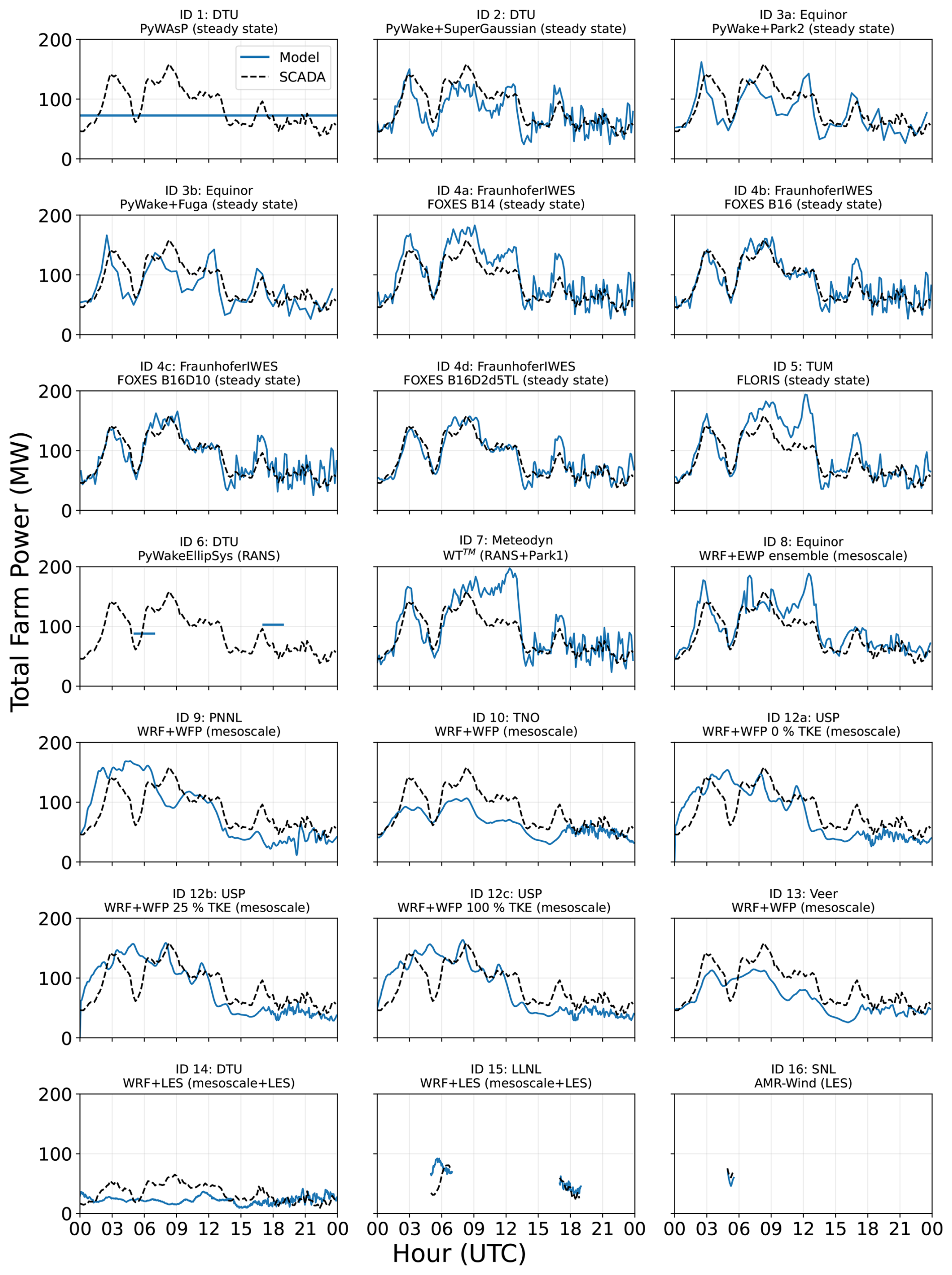
Figure 2 Time series of modeled and observed power at the King Plains wind farm on 24 August 2023 for each Phase 1 benchmark submission. Note that for submissions modeling only a subset of the turbines, the observed and modeled totals are calculated using only the corresponding turbines. Across all submissions, observed data are plotted at 10 min resolution to increase readability. For the same goal, LES-modeled data are plotted using 2 min instantaneous values.

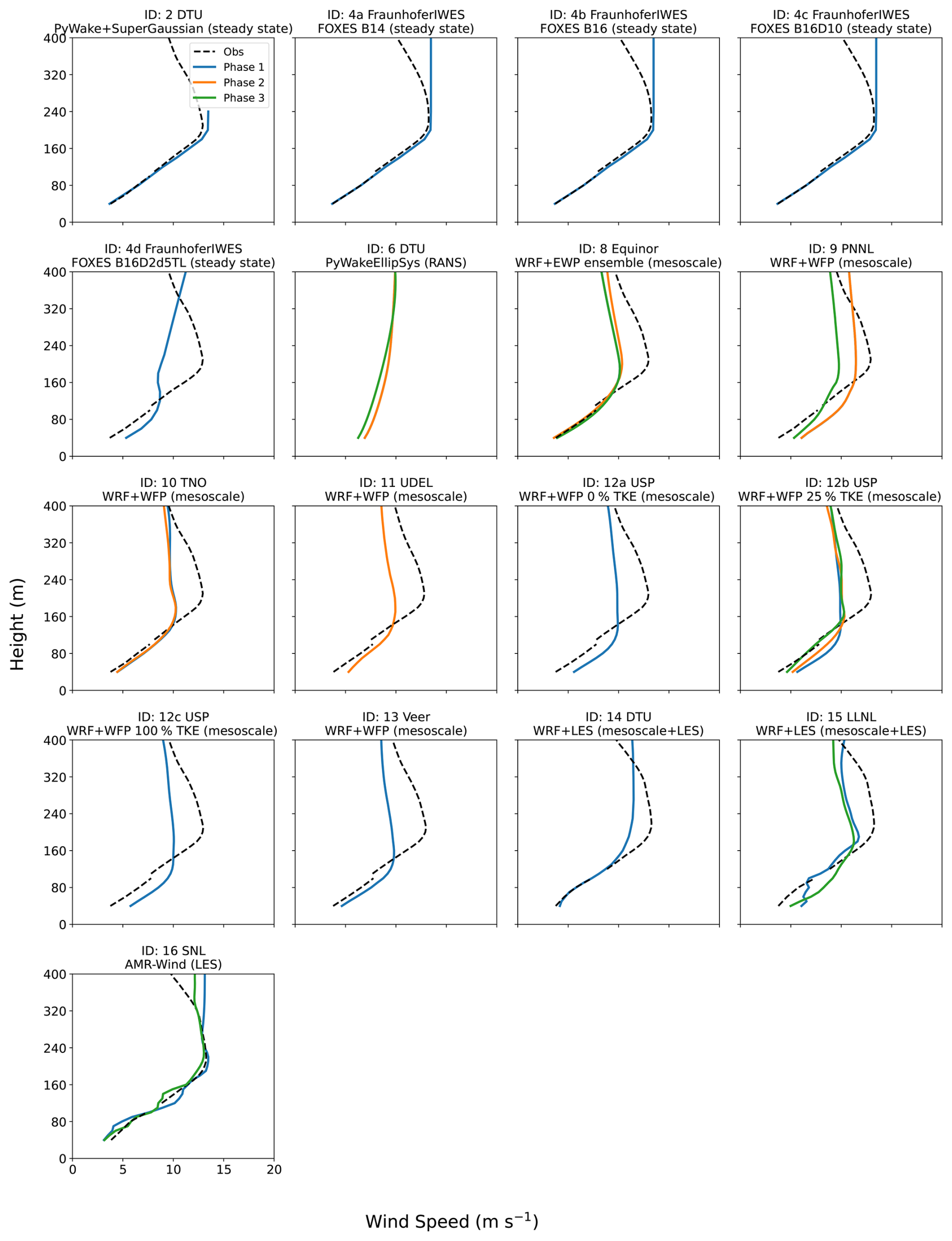
Figure 3 Modeled and observed wind speed profiles at Site A1 at 06:00 UTC on 24 August 2023. Profiles transition from profiling lidar data (≤100 m a.g.l.) to scanning lidar measurements (>100 m a.g.l.); the discrepancy at this interface represents the inherent measurement uncertainty during instrument hand-off. Observations are matched to the time resolution (and average vs. instantaneous) of each model submission. Only models that submitted wind speed information at Site A1 are included in the plot. Meteodyn WT™ results are not included as the model is designed to provide long-term mean wind profiles, not instantaneous snapshots.

To understand the physical drivers behind the discrepancies observed in the time series, we examine the observed and modeled vertical structure of the wind flow during a critical time (06:00 UTC) in stable conditions. As detailed in Part 1 (Bodini et al., 2026), this period is characterized by a strong low-level jet (LLJ) interacting with the turbine rotor layer, where jet lifting leads to a drop in power production. Wind speed profiles at Site A1 reveal significant discrepancies between models and observations during this period (Fig. 3). Because Phase 1 only provided observations of wind speed at Site A1 up to 240 m a.g.l., simpler models (e.g., PyWake + SuperGaussian and FOXES) that directly ingested these data matched the lower profile well but suffered from extrapolation errors aloft. In the absence of upper-level observations, these models often assumed profile shapes that deviated significantly from the actual LLJ structure. Some other models used monotonically increasing profiles that did not reflect the observed conditions. Conversely, WRF-based models relying on reanalysis forcing consistently underestimated the LLJ strength and placed the jet nose at a lower altitude than observed. This general inability to accurately resolve the inflow shear profile under real-world scenarios is a primary driver of the power production errors.

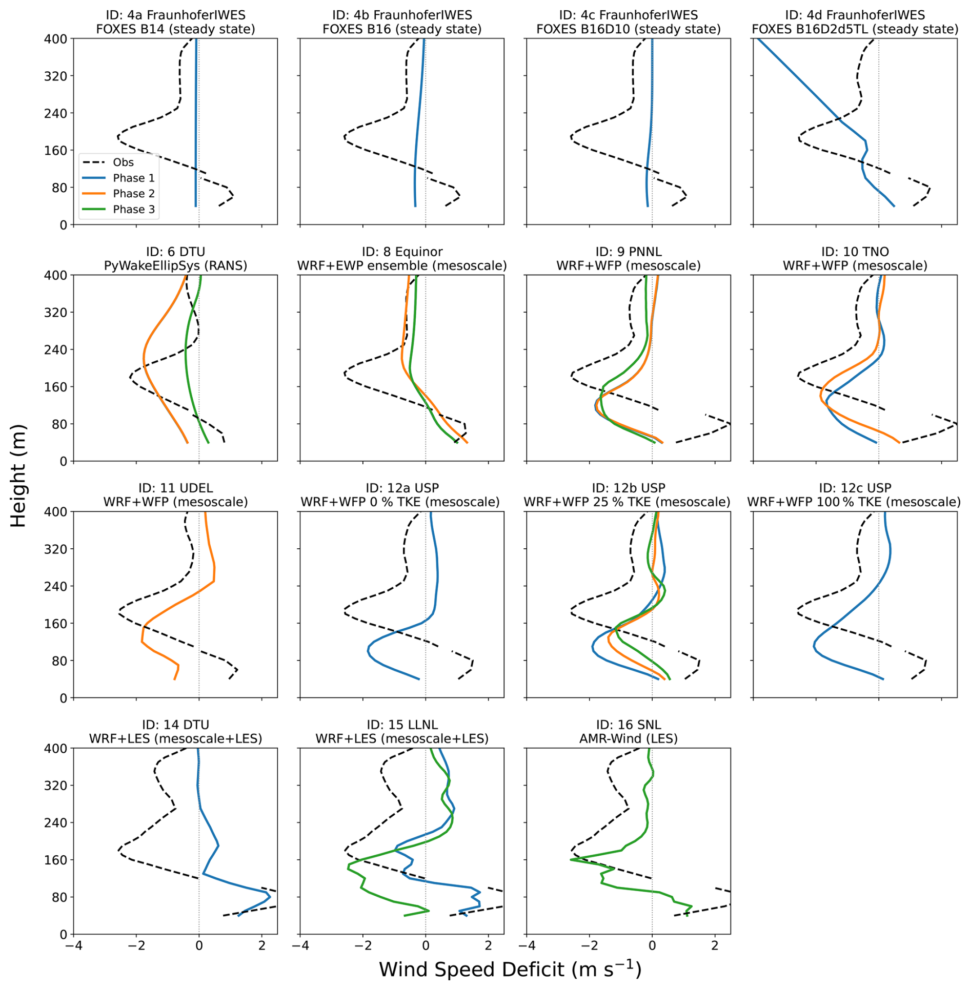
Figure 4 Modeled and observed wind speed deficit profiles, calculated as the difference between wind speed at sites H and A1, at 06:00 UTC on 24 August 2023. Observations are processed to match the time resolution and temporal treatment (averaged versus instantaneous) of each model submission and may therefore appear different across panels. Profiles transition from profiling lidar data (≤100 m a.g.l.) to scanning lidar measurements (>100 m a.g.l.). Only models providing data at both sites are shown. Meteodyn WT™ results are not included as the model is designed to provide long-term mean wind profiles, not instantaneous snapshots.

These upstream inflow deficiencies propagated downstream, complicating the resolution of wind speed profiles downwind of the wind farm, as wake effects and terrain interactions added further complexity to the flow. At Site H, located approximately 22 rotor diameters downwind, observations reveal a complex vertical structure (Fig. 4): a clear wind speed deficit aloft and flow acceleration near the surface, which is a phenomenon consistent with long-term observations at this site (Bodini et al., 2021). Given that the deficit is most pronounced above hub height, this feature is likely attributable to the terrain- and wind farm-induced lifting of the LLJ identified in Bodini et al. (2026), rather than wake effects alone. Capturing this deficit proved difficult for most models. Steady-state and most RANS approaches generally struggled to reproduce the specific nosed-deficit profile shape characteristic of the LLJ. This difficulty is rooted in a fundamental limitation: the stable period was characterized by a very shallow atmospheric boundary layer, placing the turbine rotor layer largely above the surface layer to which Monin–Obukhov Similarity Theory strictly applies. Standard turbulence closures for both RANS and engineering wake models rely heavily on equilibrium boundary layer assumptions that break down under these non-idealized, real-world conditions. The PyWakeEllipSys RANS approach was able to maintain the nosed-deficit profile, though at heights above those observed, possibly because the inflow ABL height was set to a higher value compared to the inflow data to maintain numerical stability, as discussed in Sect. 3.6. Consequently, the results of this benchmark highlight a critical research need for the community: the development and validation of improved turbulence closures capable of resolving non-equilibrium dynamics and real-world low-level-jet interactions that are frequently encountered in operational wind energy environments. WRF-based and LES submissions generally captured the presence of the nosed deficit but struggled to correctly predict its vertical height and intensity, mirroring their difficulties with the upstream inflow profile. Notably, however, some WRF submissions and all LES-based models were able to capture the flow acceleration closer to the surface.

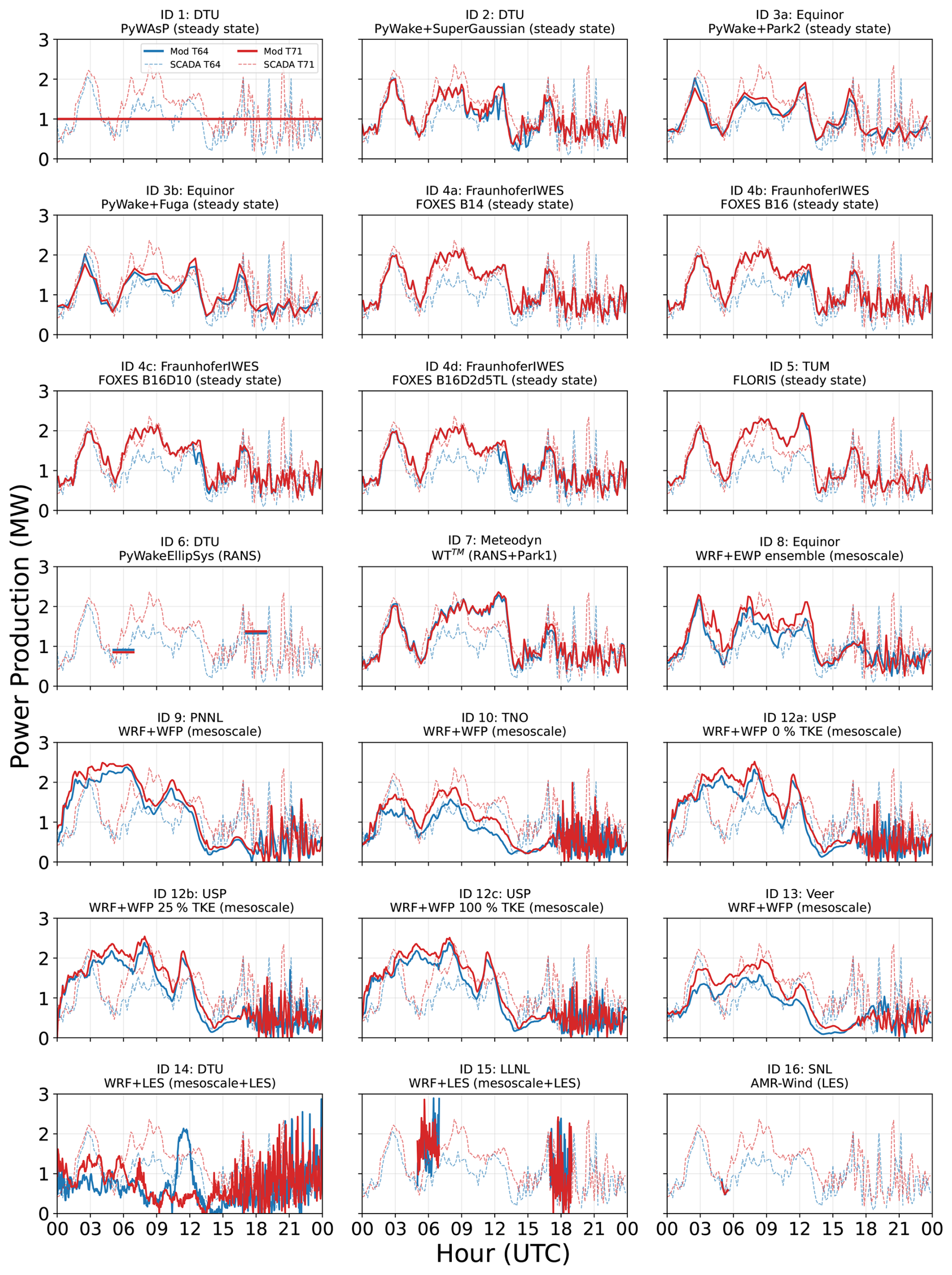
Figure 5 Time series of modeled and observed power at two selected inflow turbines (IDs 64 and 71; see map in the Part 1 paper) within the King Plains wind farm on 24 August 2023 for each Phase 1 benchmark submission. Across all submissions, observed data are plotted at 10 min resolution to increase readability. For the same goal, LES-modeled data are plotted using 2 min instantaneous values.

Correctly characterizing freestream conditions proved to be a prerequisite for accurate farm modeling. To isolate this “inflow error floor”, we examine the power production of turbines 64 and 71 (highlighted in cyan in the map in Fig. 1), which are located in the southernmost (inflow) row and do not experience internal farm wakes under southerly flow. The comparison of modeled and observed power for these turbines (Fig. 5) reveals a widespread inability to capture the spatial heterogeneity of the inflow. Despite being separated by only 3 km in relatively simple terrain, observations show that turbine 71 (dashed red line) frequently produces more power than turbine 64 (dashed blue line) during stable conditions: between 08:00 and 09:00 UTC turbine 71 output about 1 MW more power than turbine 64. Most mesoscale and LES-based models fail to track these sharp power fluctuations and the observed spatial variability, often overestimating production by more than 1 MW during the LLJ interaction between 04:00 and 06:00 UTC and, more broadly, in stable conditions. While simpler steady-state models driven by point measurements can follow the general trend of the observations, they often fail to differentiate between the two turbines, predicting nearly identical power for both. This spatial heterogeneity in the observed inflow – and the models' general inability to reproduce it – suggests that a substantial portion of the total benchmark error is inherited from the inflow specification rather than wake physics alone.

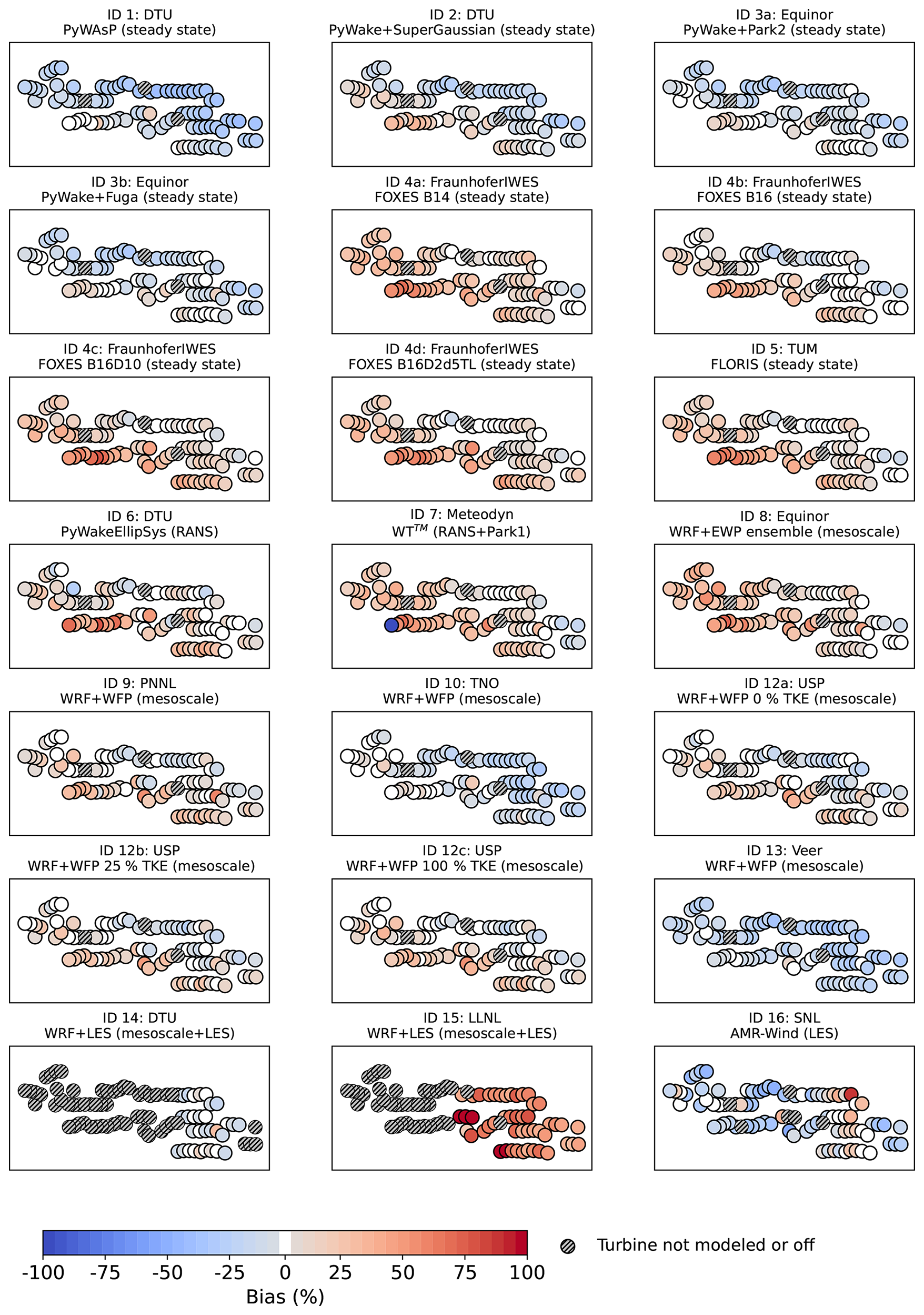
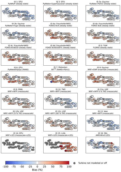
Figure 6 Maps showing the percentage bias in modeled vs. observed power produced by each turbine in the King Plains wind farm on 24 August 2023 for each model submission to Phase 1 of the benchmark.

Expanding the analysis to the full array reveals substantial inter-model variability in power bias across the wind farm (Fig. 6). Model complexity was not a primary predictor of accuracy; high-fidelity models, such as LES or mesoscale-coupled approaches, did not uniformly outperform simpler engineering or steady-state models in terms of bias. It is important to note, however, that this comparison conflates inflow characterization strategy with wake physics fidelity. Engineering models benefited from direct ingestion of high-quality point observations at Site A1, effectively site-calibrating their inflow, while mesoscale and LES models were required to derive inflow conditions from reanalysis products without such grounding. The apparent underperformance of higher-fidelity tools is therefore primarily a consequence of the inflow specification challenge rather than pure inadequacies in their wake physics representation. In fact, LES models face an additional structural challenge: they are frequently driven by mesoscale model outputs that lack resolved turbulence content. Generating realistic, turbulent, site-specific inflow conditions for LES – particularly for terrain-driven flows where periodic boundary conditions or simplified precursor methods are inadequate – remains an open and important research problem. The variable performance of LES submissions in this benchmark partly reflects these inflow generation challenges rather than deficiencies in the LES wake physics itself. Variability is evident not only across different modeling approaches but also within the same family of models (e.g., the various WRF submissions), highlighting the high sensitivity of results to user-defined configurations such as the reanalysis product, PBL scheme, or grid resolution. Furthermore, a systematic spatial trend is observable across the majority of submissions: turbines in the southwestern region generally exhibit positive (or less negative) biases, while turbines in the northeastern sector show distinct negative (or less positive) biases. This southwest–northeast gradient suggests a widespread difficulty in capturing the spatial heterogeneity of the flow field across the site, likely driven by the complex terrain-flow interactions described in the Part 1 paper (Bodini et al., 2026) and in Radünz et al. (2025).

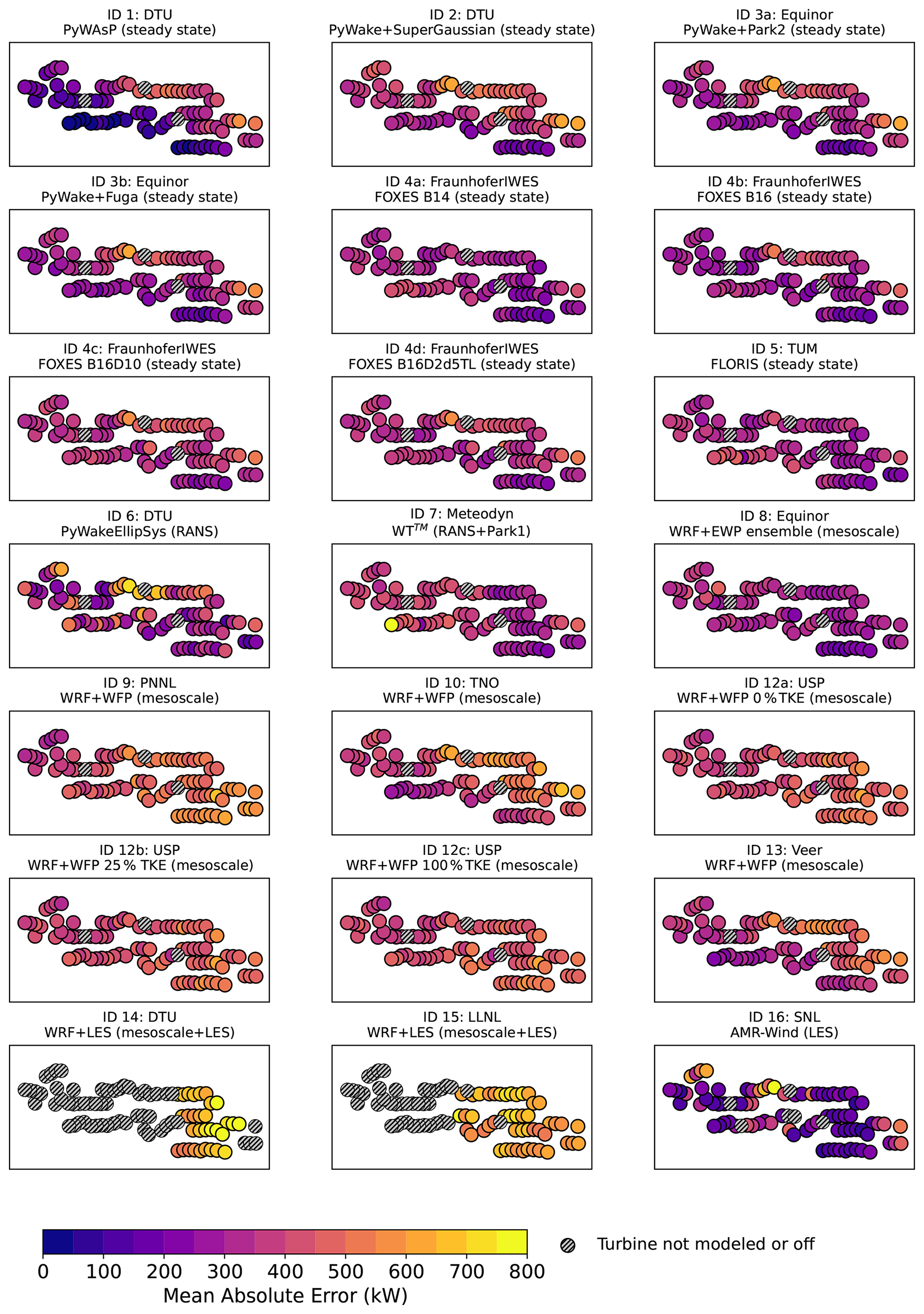
Figure 7 Maps showing the mean absolute error in modeled vs. observed power produced by each turbine in the King Plains wind farm on 24 August 2023 for each model submission to Phase 1 of the benchmark.

Because bias metrics can mask performance issues through error compensation, we also examine the mean absolute error (MAE) in turbine-level power production (Fig. 7). Consistent with the bias results, significant variability exists across model types. The spatial analysis reveals that waked turbines generally exhibit higher MAE values compared to freestream turbines, reflecting the added complexity of accurately resolving wake deficits and recovery compounded by terrain-induced acceleration effects.

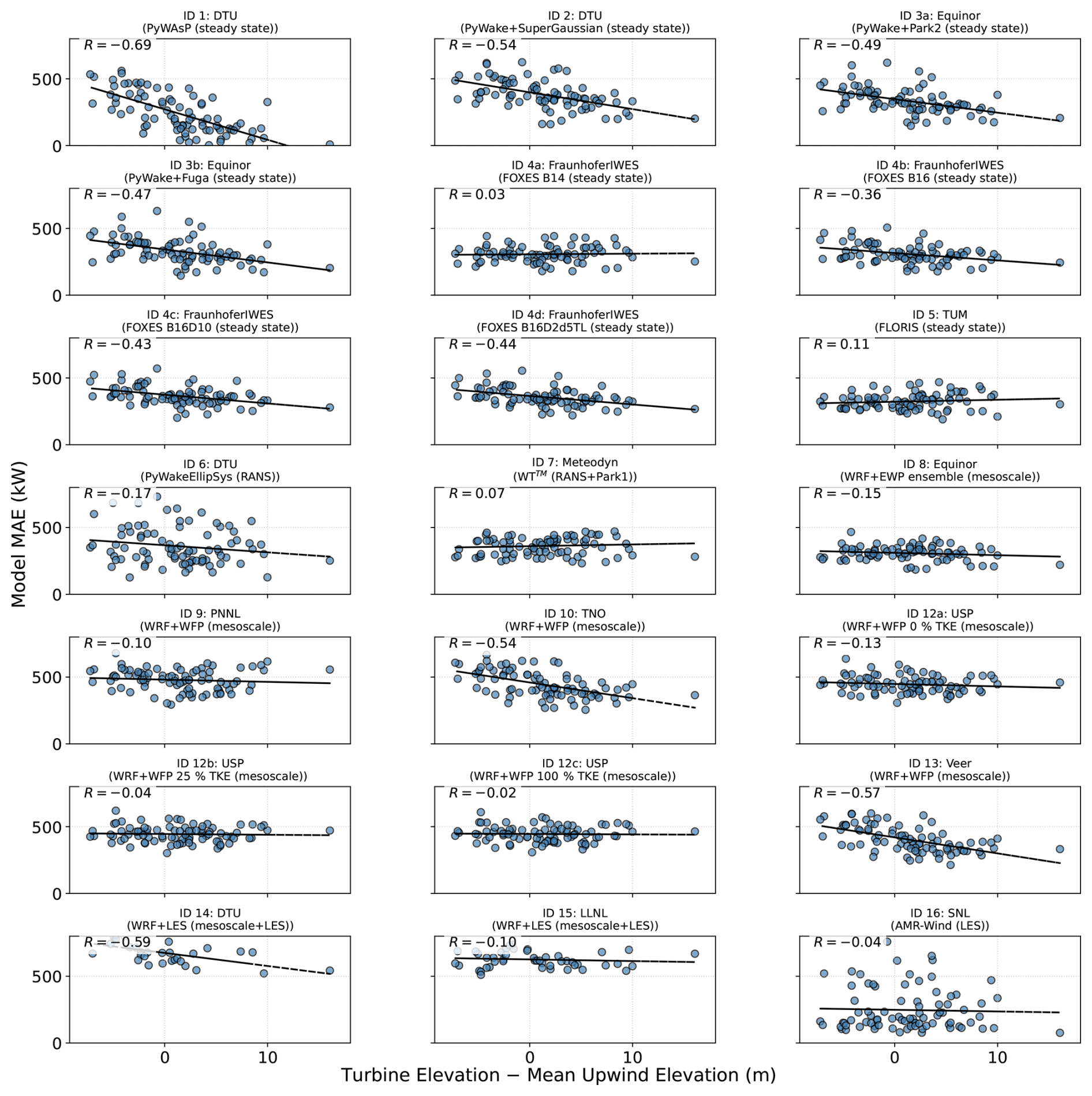
Figure 8 Scatterplots of turbine-level MAE vs. relative terrain elevation for each Phase 1 model submission.

The spatial patterns in bias and MAE point to a strong topographic influence on model performance. As noted in the Part 1 analysis (Bodini et al., 2026) and in Radünz et al. (2025), observational data revealed a counterintuitive phenomenon where turbines in the waked rows of the King Plains wind farm produced higher power output, attributed to terrain-induced flow acceleration. To quantify this topographic influence, we define a relative elevation metric Δz_rel for each turbine as

$$\begin{array}{}\text{(3)}& \mathrm{\Delta }{z}_{\mathrm{rel}}=z_{\mathrm{turbine}}-{\stackrel{\mathrm{‾}}{z}}_{\mathrm{upstream}},\end{array}$$

where z_turbine is the actual physical base elevation of the turbine and ${\stackrel{\mathrm{‾}}{z}}_{\mathrm{upstream}}$ is the mean physical terrain elevation within a 1 km upstream sector (defined by a 45° arc centered on the mean hub-height wind direction). A negative Δz_rel indicates the turbine is situated in a local depression or at the base of a downward slope relative to the upwind terrain, while a positive value indicates a local topographic high, such as a ridge. Plotting turbine-level MAE against Δz_rel reveals a prevalent negative correlation across the majority of submissions (Fig. 8). This indicates that models exhibit higher errors at turbines situated at elevations lower than the upstream terrain, confirming the difficulty in capturing the interaction between wakes and terrain-induced speed-ups. This negative correlation is generally stronger for stable conditions (Fig. S1 in the Supplement), while most models show weaker correlations (sometime even positive) during turbulent, unstable conditions (Fig. S2). While most engineering models generally show strong negative correlations, results for higher-fidelity approaches are mixed. The FLORIS submission shows a weak positive correlation in Phase 1, deviating from the general trend. However, as shown in the Supplement (Figs. S3 and S4), this correlation shifts to negative in subsequent benchmark phases, suggesting that as inflow errors are corrected via model calibration, the underlying terrain-induced physics becomes the dominant remaining source of spatial error. Beyond the challenge of terrain representation, this result also exposes a fundamental difficulty in LES: the near-wall region over terrain is typically modeled rather than directly resolved. Classical wall models that rely on the logarithmic law of the wall are known to break down in terrain-driven flows such as the terrain-induced accelerations documented here, highlighting the critical need for improved near-wall models for LES in wind energy applications.

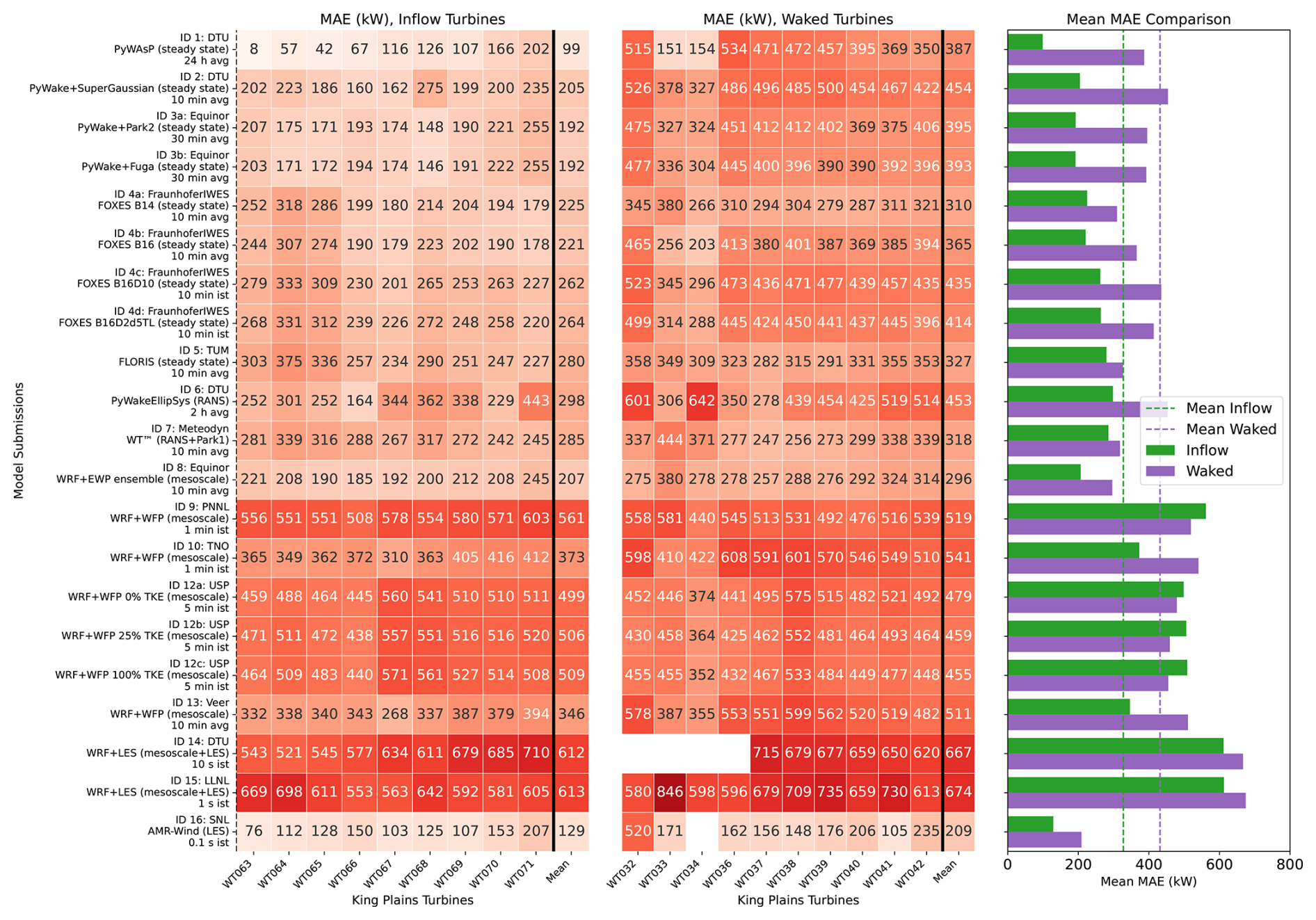
Figure 9 MAE in modeled power for selected turbines in the southern (inflow) row of King Plains (left) and the northern (waked) row (middle). The bar chart on the right compares the mean MAE across all submissions for inflow vs. waked turbines. Results for Phase 1.

The significant impact of local topography reinforces the observation made earlier in this section: substantial prediction errors persist even for turbines unaffected by upstream wakes. To weigh the relative contributions of these baseline errors (driven by terrain and inflow specification) versus wake physics to the total error, we compare the aggregate MAE for inflow and waked turbines (Fig. 9). Across all Phase 1 submissions, the mean MAE for inflow turbines exceeded 300 kW (∼11 % of the nameplate capacity), while the mean MAE for waked turbines averaged over 400 kW (∼14 % of the nameplate capacity). This comparison indicates that difficulties in accurately representing inflow conditions contribute significantly to the total error, suggesting that wake modeling inaccuracies are not the sole, or perhaps even the primary, driver of performance losses in real-world terrain-driven flows. Interestingly, a subset of the WRF-based models exhibits near-equal or even lower error for waked turbines than for inflow turbines. This result reinforces the conclusion that for mesoscale approaches, prioritizing improvements in inflow representation – potentially through better ensemble selection or data assimilation – may yield larger accuracy gains than focusing on wake parameterization alone. Finally, the data highlight substantial variability in model results between neighboring wind turbines; these localized discrepancies point to microscale terrain features or complex wake interactions that remain difficult to capture consistently.

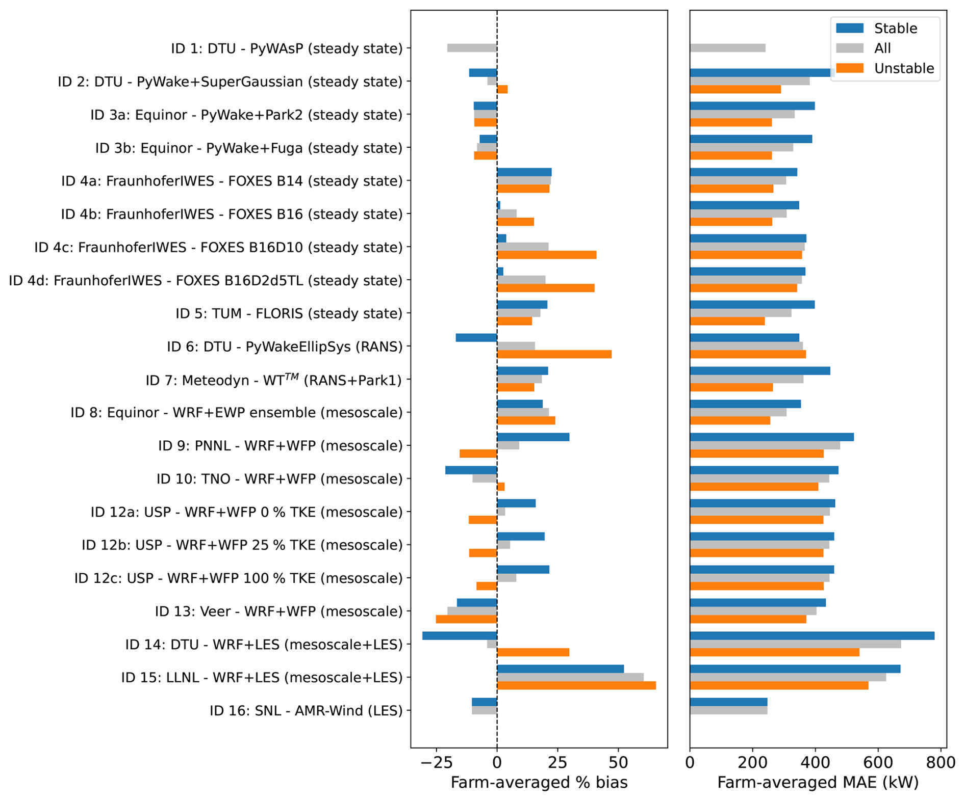
Figure 10 Histograms showing the farm-averaged percentage bias (left) and MAE (right) in modeled vs. observed power produced by the King Plains wind farm on 24 August 2023 for each model submission to Phase 1 of the benchmark.

Segregating performance by atmospheric stability (using the Obukhov length calculated from sonic anemometer measurements at Site A1) further highlights the physical challenges faced by the models (Fig. 10). Generally, models exhibited higher MAE under stable conditions, consistent with the difficulties of resolving shallow mixing depths, strong shear, and terrain-induced accelerations in the stable boundary layer. While the farm-averaged bias metric displays no clear systematic trend across all models favoring one stability class, the results reveal a critical trade-off between systematic bias and absolute error in time-resolved modeling. Notably, the DTU WRF + LES submission achieves a near-zero bias for the complete period (driven by a compensating effect between a large negative bias in stable conditions and a large positive bias in unstable conditions) yet exhibits the highest MAE of all participants. This discrepancy, shared by other high-fidelity submissions, illustrates the “double penalty” effect inherent to simulations resolved at fine time resolution: unavoidable phase errors in simulating high-frequency wind fluctuations increase the absolute error, whereas steady-state models that target the mean flow circumvent these timing penalties, often resulting in lower MAE despite potentially larger systematic biases.

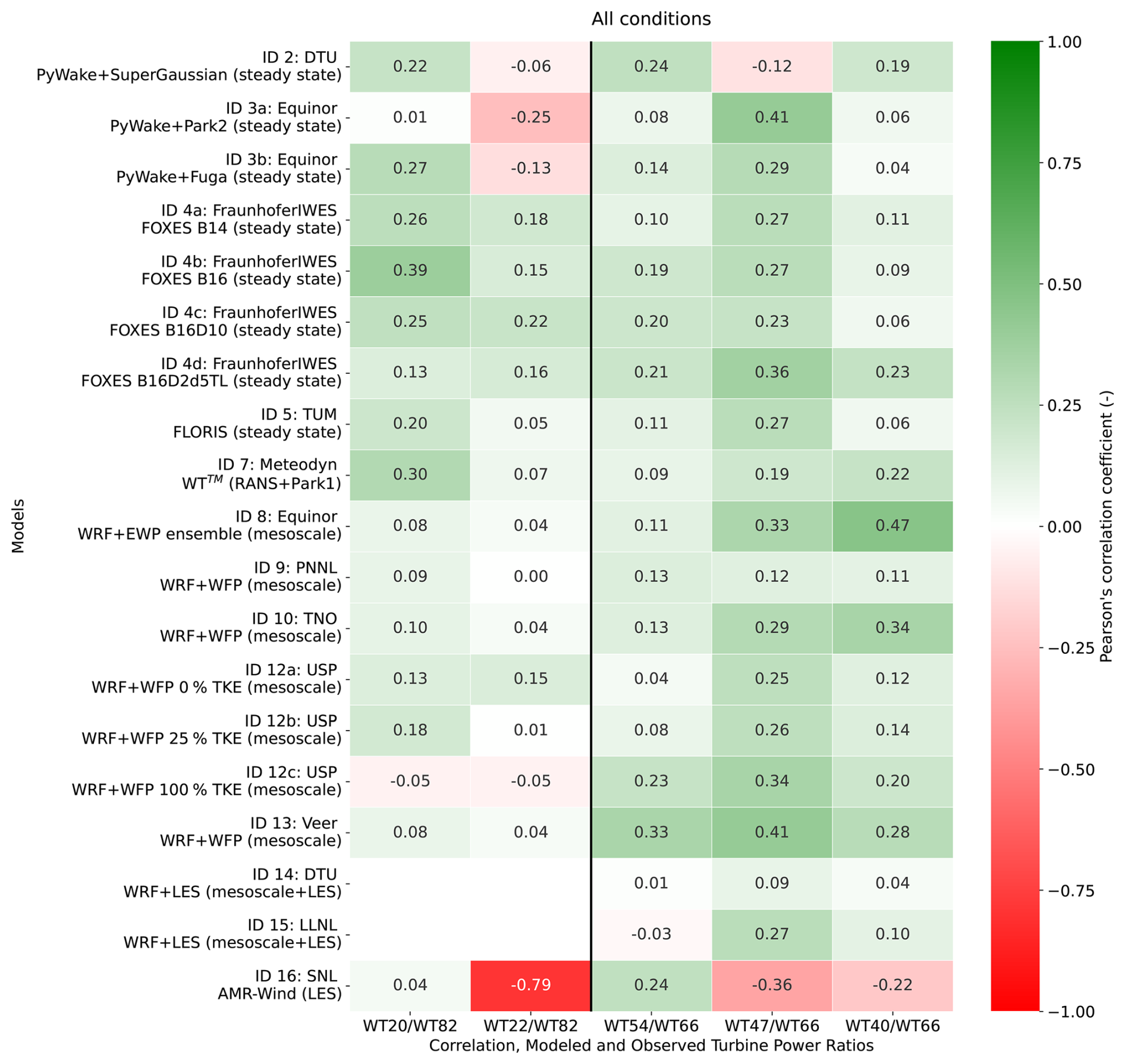
Figure 11 Pearson correlation coefficients between observed and modeled power ratios for selected turbine pairs during Phase 1. The ratios are calculated as the power of the waked turbine divided by the power of a corresponding upstream reference turbine in the southernmost row, for turbines in the western (left) and eastern (right) portions of King Plains.

Finally, to isolate the internal physics of wake propagation from inflow errors, we computed correlations between observed and modeled power ratios for selected turbine pairs (Fig. 11). For this analysis, each ratio is defined with a waked turbine in the numerator and an upwind turbine (located in the southernmost row) in the denominator. The selected turbines are highlighted in orange (western transect) and green (eastern transect) in the map in Fig. 1. Overall, the resulting correlations are relatively low, indicating that capturing the specific temporal dynamics of wake losses remains a challenge for most modeling approaches. However, under stable conditions (Fig. 12) – which are characterized by less chaotic flow and reduced turbulence – correlations increase across the board, even though the MAE is generally higher in these regimes. This distinction underscores that while errors in inflow and terrain representation dominate the absolute power prediction, the relative wake dynamics are better resolved during stable stratification, likely because the reduced ambient turbulence leads to more persistent wake structures that are less obscured by meandering and mixing. In contrast, the lower correlations observed in unstable conditions (Fig. S5 in the Supplement) reflect the inherent difficulty of tracking high-frequency turbulent fluctuations in the time domain. Spatially, most models consistently exhibit higher correlations for specific turbine pairs, such as those associated with Turbine 20 (second row, western sector) and Turbine 47 (third row, eastern sector). Notably, we observe no systematic reduction in correlation strength in the western portion of the farm, suggesting that the external farm-to-farm wakes from Armadillo Flats did not significantly degrade the models' ability to capture relative wake dynamics compared to the eastern section.

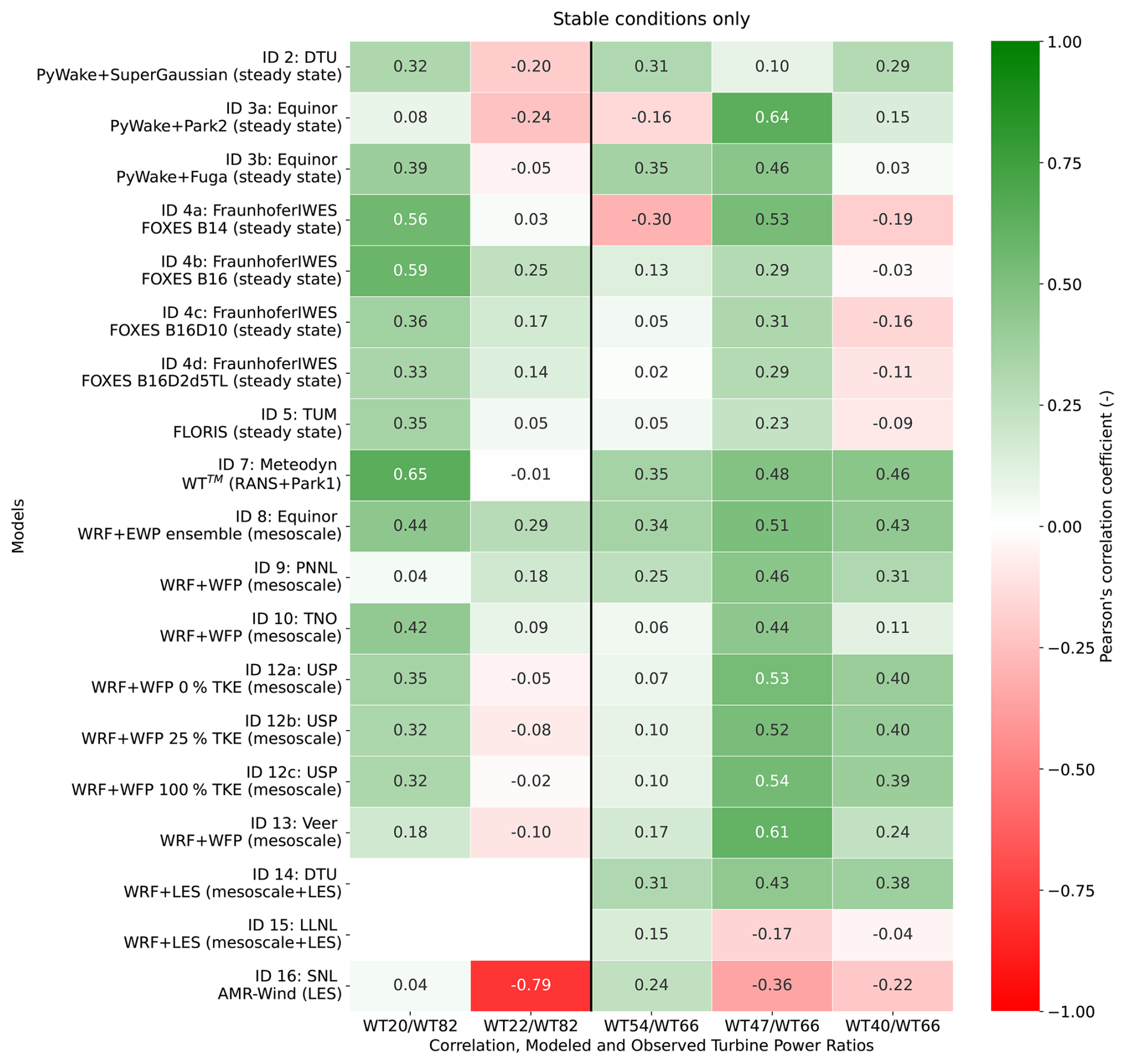
Figure 12 Pearson correlation coefficients between observed and modeled power ratios between turbine pairs during Phase 1, calculated using only data from stable atmospheric conditions, for turbines in the western (left) and eastern (right) portions of King Plains.

4.2 Evolution of model errors through Phases 2 and 3

In Phases 2 and 3, modelers were provided with progressively richer observational datasets, culminating in the release of SCADA data for all King Plains turbines for the benchmark day in Phase 3. The modeled wind speed profiles at Site A1 (Fig. 3) exhibited only limited variations in Phases 2 and 3 compared to the baseline, reflecting the constraints many models face in directly assimilating single-point profile observations. However, more distinct variations are evident in the modeled wind speed deficit profiles (Fig. 4), suggesting that updates to model setups, such as calibration or refined boundary conditions, had a more pronounced impact on the representation of wake recovery.

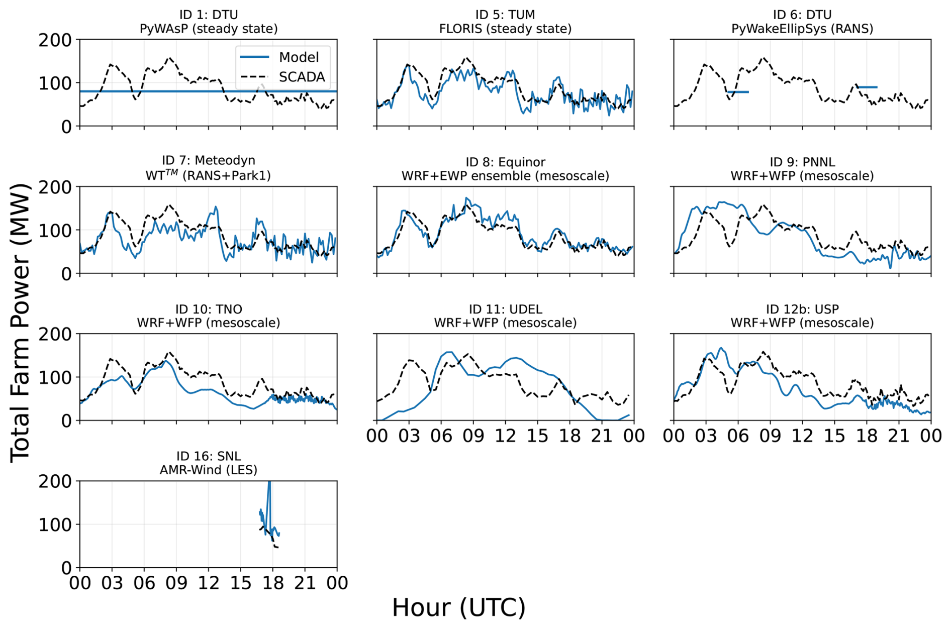
Figure 13 Time series of modeled and observed power at the King Plains wind farm on 24 August 2023 for each Phase 2 benchmark submission. Note that for submissions modeling only a subset of the turbines, the observed and modeled totals are calculated using only the corresponding turbines. Across all submissions, observed data are plotted at 10 min resolution to increase readability. For the same goal, LES-modeled data are plotted using 2 min instantaneous values.

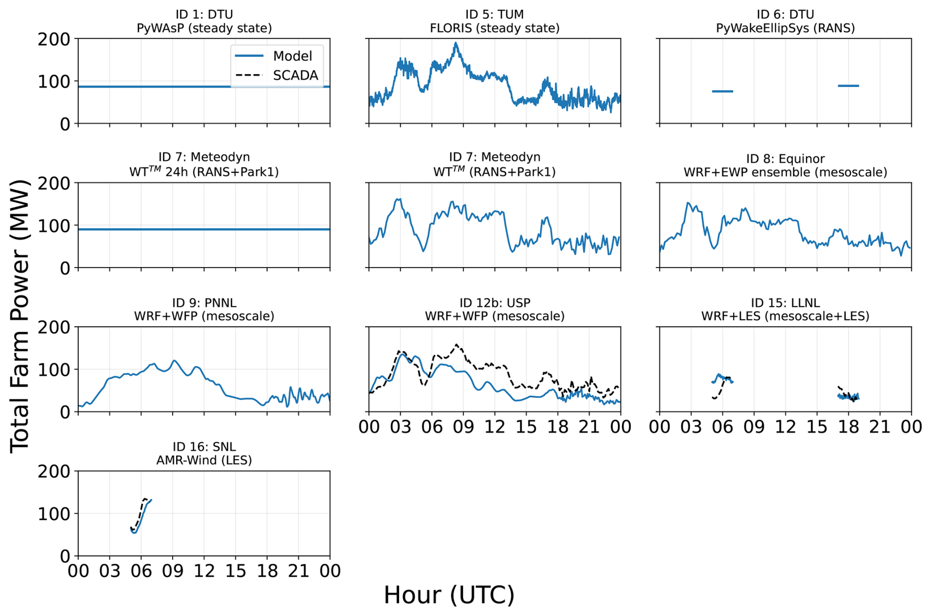
Figure 14 Time series of modeled and observed power at the King Plains wind farm on 24 August 2023 for each Phase 3 benchmark submission. Note that for submissions modeling only a subset of the turbines, the observed and modeled totals are calculated using only the corresponding turbines. Across all submissions, observed data are plotted at 10 min resolution to increase readability. For the same goal, LES-modeled data are plotted using 2 min instantaneous values.

The impact of this additional data access on model performance is first examined through the time series of farm-level power production shown in Figs. 13 and 14. Phase 2 results show a general improvement over the baseline (Fig. 13). Access to detailed inflow atmospheric data and SCADA from inflow turbines allowed participants to refine their boundary conditions and internal parameters. For instance, the FLORIS simulation showed improved agreement with observations, effectively filtering out the unrealistic peaks observed in Phase 1. However, challenges persisted for mesoscale models, which continued to struggle with the sharp power drop associated with the LLJ lifting at 05:00 UTC. In Phase 3, the release of full SCADA data enabled direct model calibration, leading to significant performance gains (Fig. 14). The FLORIS model, now tuned to the provided power data, achieved a remarkable match with observations. Physics-based models also demonstrated marked improvements; the RANS submission by Meteodyn, the WRF submission by Equinor, and the steady-state PyWAsP model by DTU all achieved high accuracy. The Sandia LES model also performed well. It is important to note that the performance gains observed in Phase 3 should be interpreted as conditional error minimization rather than evidence of generalizable predictive capability. Models in this phase had access to the full observational dataset for the case study day, including all SCADA power outputs and inflow measurements. The resulting improvements therefore reflect the models' ability to adapt to a well-constrained and fully observed atmospheric state, not necessarily their ability to forecast that state independently. This distinction is critical for operational applications, where such comprehensive in situ data are unavailable a priori. Closely related to this point, the strong Phase 3 performance of models employing spatially heterogeneous parameter adjustments stems from localized tuning that effectively absorbs unresolved physical processes – including terrain-induced flow modifications and stability effects – into empirical corrections anchored to this specific case study. While highly effective for reconstructing the observed day, the transferability of such parameter sets to different atmospheric conditions, seasons, or wind directions has not been established here and represents an important open question.

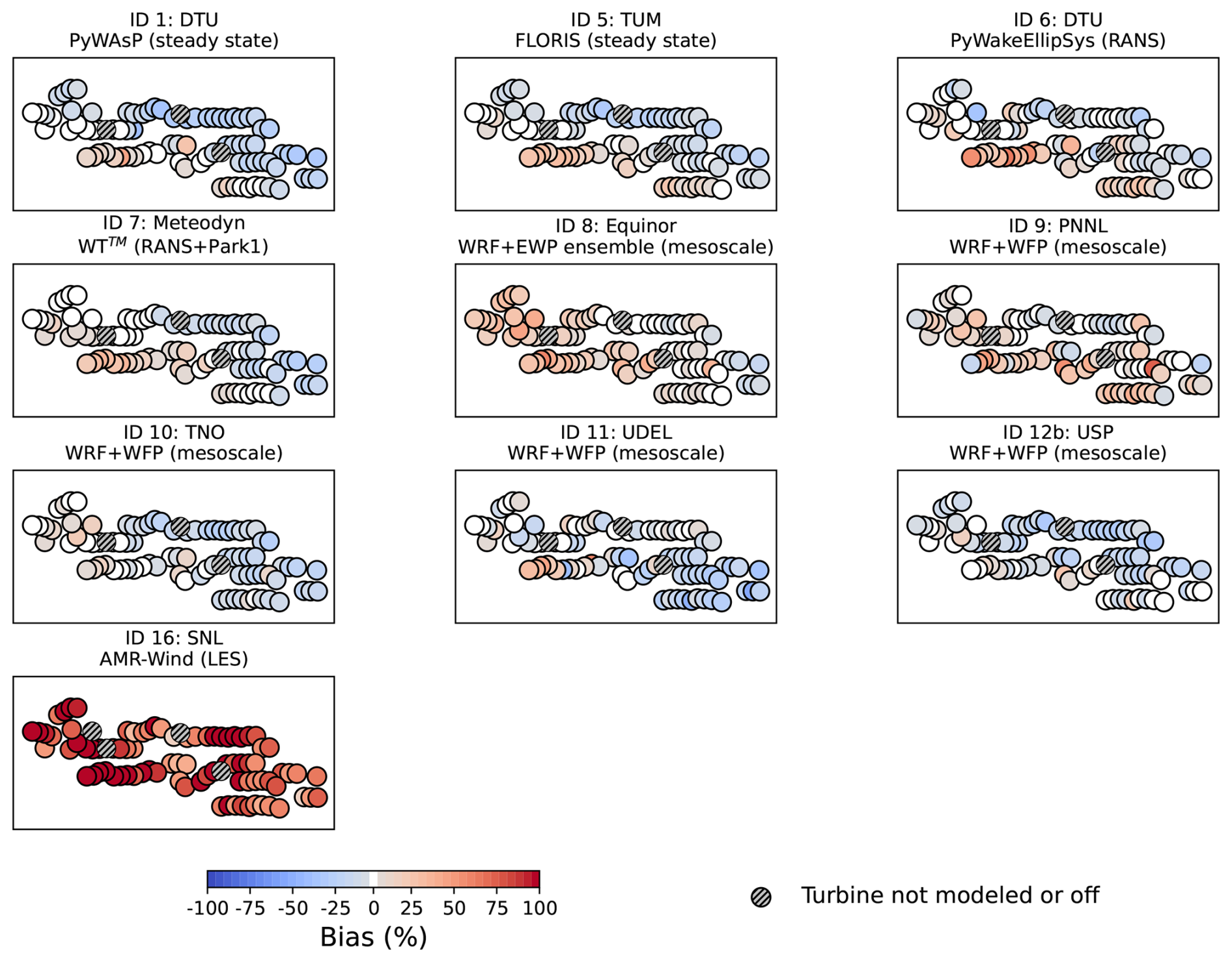
Figure 15 Maps showing the percentage bias in modeled vs. observed power produced by each turbine in the King Plains wind farm on 24 August 2023 for each model submission to Phase 2 of the benchmark.

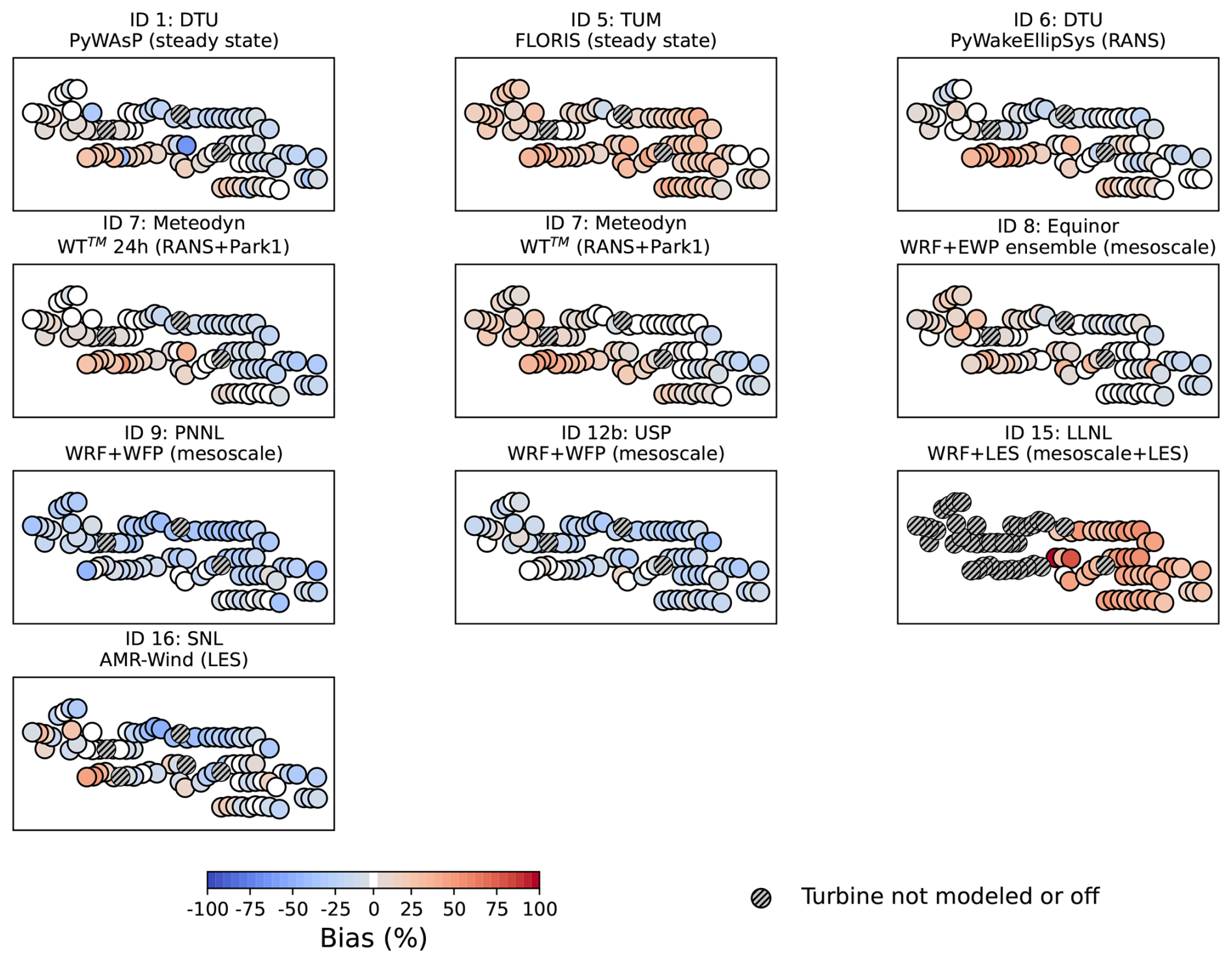
Figure 16 Maps showing the percentage bias in modeled vs. observed power produced by each turbine in the King Plains wind farm on 24 August 2023 for each model submission to Phase 3 of the benchmark.

While spatial variability persists, specific models demonstrated marked improvements in bias reduction as participants leveraged the additional data (Figs. 15 and 16). For example, the availability of detailed inflow profiles allowed for corrections in background flow fields that mitigated some of the spatial gradients observed in Phase 1, particularly for models capable of directly assimilating observational data rather than relying solely on reanalysis forcing. It is important to note that the Sandia submission (AMR-Wind) modeled a different temporal window in Phase 2 (unstable conditions) compared to Phase 1 (stable conditions), resulting in a distinct error distribution for that specific submission.

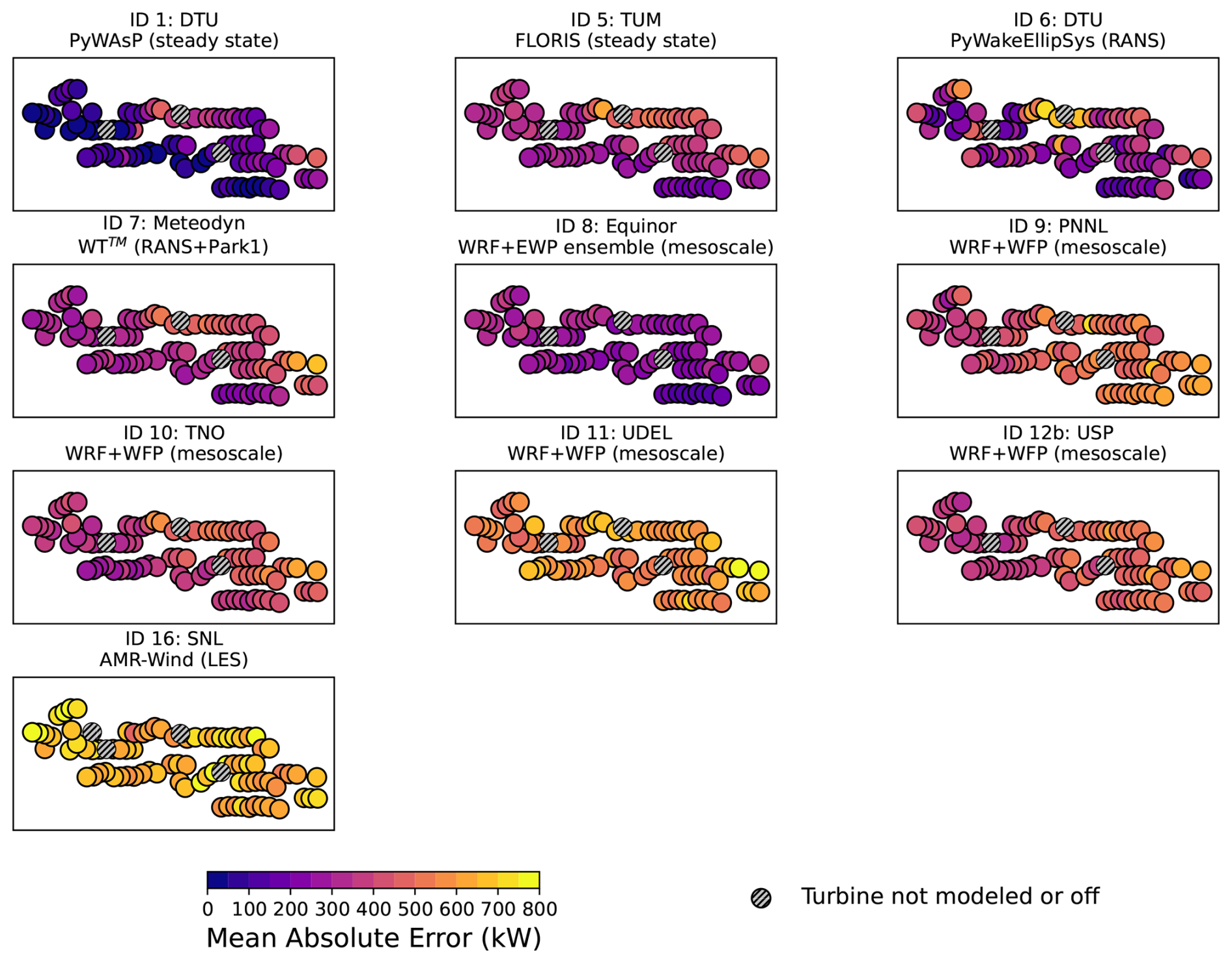
Figure 17 Maps showing the mean absolute error in modeled vs. observed power produced by each turbine in the King Plains wind farm on 24 August 2023 for each model submission to Phase 2 of the benchmark.

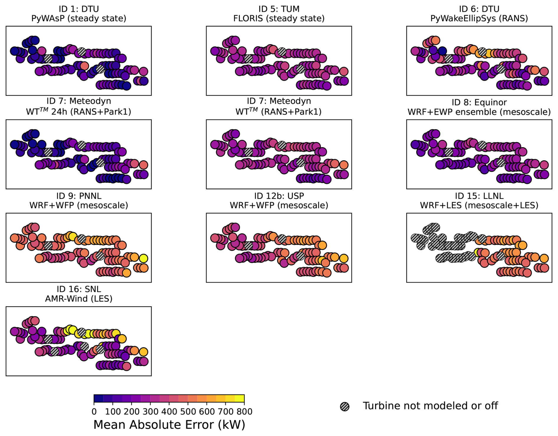
Figure 18 Maps showing the mean absolute error in modeled vs. observed power produced by each turbine in the King Plains wind farm on 24 August 2023 for each model submission to Phase 3 of the benchmark.

The evolution of MAE through Phases 2 and 3 confirms that the majority of models achieved a reduction in error (Figs. 17 and 18). However, a persistent spatial pattern remained for most participants, characterized by larger MAE values in the waked portion of the wind farm compared to the inflow row. When looking at MAE values for selected inflow and waked turbines in the eastern (unwaked by Armadillo Flats) portion of the King Plains wind farm (Figs. S6 and S7 in the Supplement), the error in modeled power for the inflow turbines still accounts for about two-thirds of the error seen for the waked turbines, on average. A notable exception was observed in the University of Delaware's submission (WRF with a customized WFP); in Phase 2, this model successfully mitigated the high bias previously observed in the northeastern portion of the farm, likely due to a refined calibration of the TKE parameterization. As already noted in Phase 1, most models had larger MAE values in stable conditions in Phases 2 and 3 (Figs. S8 and S9), but stable conditions also exhibited higher correlations with observations of power once normalized by inflow turbine productions (Figs. S10 through S15).

A key outcome of this benchmark is the quantification of model improvement enabled by access to additional observations. Figure 19 illustrates the reduction in MAE for participants who submitted results in both Phases 1 and 3. Most models achieved lower MAE, with one participant improving by over 40 %. While these gains are scientifically valuable for diagnosing model behavior and calibration potential, they are best understood as upper bounds on achievable accuracy under ideal observational conditions rather than as estimates of operational forecast skill. These gains were achieved through distinct strategies detailed in Sect. 3 as follows.

• Calibration: Technical University of Munich (FLORIS) and Meteodyn utilized the released wake and SCADA data to calibrate wake decay parameters and tune their models to the specific site conditions.

• Ensemble selection: Equinor (WRF + EWP) refined their ensemble approach by selecting the optimal model member via a cost function that minimized misfit against available SCADA power and lidar wind direction data.

• Resolution and physics: Lawrence Livermore National Laboratory and University of California, Berkeley (WRF-LES) increased model fidelity by moving from two to three nested domains. Similarly, Technical University of Denmark (PyWakeEllipSys) addressed numerical artifacts in the stable case by adopting a modified ABL inflow method. Technical University of Denmark (PyWAsP) improved results by expanding the wind climate input to include multiple lidar data streams.

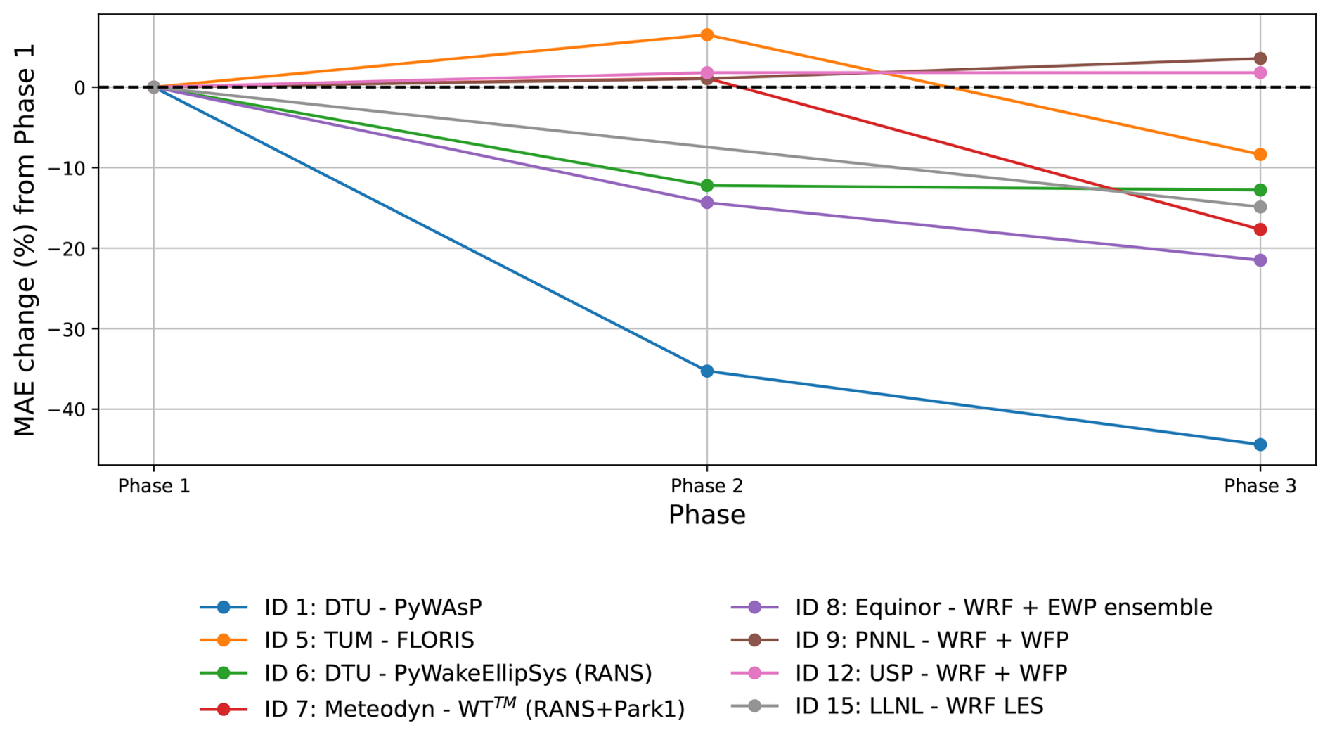
Figure 19 Change in mean absolute error over the different phases of the benchmark for those participants who submitted results in both Phases 1 and 3 of the benchmark. Note that the Sandia submission is not included in this plot as each phase simulated a different period.

5 Conclusions

The AWAKEN benchmark represents a significant community step for the validation of wind farm flow models, leveraging a uniquely rich dataset to assess model performance across a wide range of fidelities. Beyond a simple comparison of error metrics, this exercise revealed critical insights into the hierarchy of physical drivers governing wind farm performance.

A primary conclusion is that accurate characterization of inflow and terrain effects is as important as accurate wake modeling. The results highlight that increased model complexity does not automatically guarantee improved accuracy. In Phase 1, simpler engineering and steady-state models often matched or outperformed higher-fidelity approaches in terms of bulk error metrics for this specific case. This result should not be interpreted as evidence that simplified wake physics are superior to high-fidelity approaches, nor that models performing well on aggregate metrics are necessarily physically accurate. Rather, it reflects a fundamental asymmetry in inflow strategy: engineering models were site-calibrated, directly ingesting the provided in situ lidar observations, whereas mesoscale and LES models were required to predict the inflow from coarser reanalysis products (e.g., ERA5, HRRR), which failed to capture specific atmospheric features such as the exact timing and height of the nocturnal LLJ or the spatial inhomogeneity of the inflow. Consequently, high-fidelity model errors are primarily inflow errors – limitations of the boundary forcing – rather than errors in the wake physics themselves. Moreover, many simpler models assumed spatially homogeneous inflow conditions; while this assumption can yield favorable aggregate energy production estimates, it does not capture the site's true spatial heterogeneity, and agreement at the farm-integrated level may mask compensating spatial biases rather than reflecting genuine physical fidelity. Correctly characterizing freestream inflow conditions is therefore a critical – though not sufficient – step for accurate farm-level modeling. More accurate reanalysis products would substantially benefit the class of simulation tools that depend on them. From an industrial perspective, this finding has a direct and strong implication: inflow uncertainty defines a lower bound on achievable model accuracy that is independent of wake modeling fidelity. Even for turbines with negligible wake exposure, substantial prediction errors persisted throughout all phases of the benchmark, indicating that upstream atmospheric state representation – not wake parameterization – is the dominant source of uncertainty in real-world terrain-driven flows. This has immediate consequences for pre-construction energy assessment workflows and uncertainty quantification practices: investments in improving inflow characterization, whether through denser observational networks, improved data assimilation, or better mesoscale products, are likely to yield significantly larger gains in prediction accuracy than equivalent investments in wake model sophistication alone.

Furthermore, the benchmark underscored the critical role of topography, even in environments often categorized as having simple or moderate terrain. Observational data revealed that terrain-induced flow acceleration frequently outweighed wake losses, causing specific waked turbines to produce more power than those in the inflow row. Most models, regardless of fidelity, struggled to resolve this interplay between the LLJ, wakes, and local terrain-induced speed-ups. This suggests that future modeling efforts must place equal emphasis on microscale terrain resolution as they do on wake parameterization.

The multiphase structure of the benchmark demonstrated that having access to more observations is relatively effective in mitigating these sources of error. As participants gained access to site-specific inflow and wake observations, prediction errors were reduced by up to 40 % in some cases. Persistent challenges remain, particularly in modeling the interaction between atmospheric stability and wake recovery. While models struggle to capture the full temporal variability in wake interactions in unstable conditions, they perform markedly better in stable regimes when inflow variability is reduced.

From a logistical perspective, this exercise provided valuable lessons for future benchmarking initiatives. Clear instructions and standardized data submission templates are essential to ensure consistency across participants and reduce the burden of post-processing. It is also crucial to recognize the constraints of participants; limited time and resources mean that providing massive volumes of observational data does not guarantee it will all be effectively utilized. Furthermore, a structural limitation of this benchmark that must be explicitly acknowledged is its focus on a single diurnal case study. While this provides a rich and controlled test environment, it introduces the risk that model adjustments and calibrations implicitly encode features of this particular event. Consequently, the performance improvements demonstrated here cannot be directly extrapolated to annual energy production estimates or other probabilistic long-term assessments. Future benchmarks should target multi-year, climatologically representative datasets to rigorously assess model transferability.

Looking ahead, this benchmark exposes several high-priority, fundamental research challenges that the wind energy modeling community must address. Crucially, these challenges collectively define limits on model transferability, not simply areas requiring incremental improvement. First, accurate inflow characterization remains the primary limiting factor: improved data assimilation methods, denser observational networks, and more accurate mesoscale reanalysis products are needed to reduce the “inflow error floor” that this benchmark clearly demonstrates. Second, non-equilibrium boundary layer physics – including low-level jets, stability transitions, and conditions where MOST breaks down – demands improved turbulence closures that extend beyond current equilibrium assumptions. Third, generating realistic turbulent inflow for LES in heterogeneous terrain, particularly under non-periodic and non-neutral conditions, requires dedicated methodological advances. Finally, the multiscale coupling of terrain effects and wake dynamics must be treated as a first-order modeling priority rather than a secondary detail, as terrain-induced flow modifications can rival or even exceed wake losses in magnitude. Ultimately, addressing these physical and structural boundaries is essential to distinguishing models capable of truly generalizing across diverse atmospheric regimes from those that merely reconstruct a single constrained state.