Impact of atmospheric turbulence on performance and loads of wind turbines: knowledge gaps and research challenges

Wind energy harvesting from the atmosphere takes place in the atmospheric boundary layer. The boundary layer shear and buoyancy create three-dimensional turbulent eddies spanning a range of scales that form a continuous forward cascade of kinetic energy to the smallest scales of motion where energy is dissipated. Large-scale atmospheric circulations modulate the boundary layer turbulence, characterized by coherence and intermittency. As wind turbines grow in size and the integrated control of both turbines and wind farms spans greater distances, the relationship between the scales of atmospheric turbulence and the design and operation of wind energy facilities has entered new territory. The boundary layer turbulence impacts both wind turbine power production and turbine loads. Optimizing wind turbine and wind farm performance requires an understanding of how turbulence affects both wind turbine efficiency and reliability. While the characteristics of atmospheric boundary layer turbulence have been observed and studied in detail over the last few decades, there are still significant gaps in our understanding of the impact of turbulence on wind power resources and wind farm operations. This paper outlines the current state of turbulence research relevant to wind energy applications and points to gaps in our knowledge that need to be addressed to effectively utilize wind resources.

1 Introduction

Most human activity happens in the atmospheric boundary layer (ABL), which extends a few hundred meters to a couple of kilometers above the surface of the Earth. The flow in the ABL is characterized by turbulent eddies and vortices that contribute to the exchanges of momentum, heat, moisture, and other constituents between Earth's surface and the atmosphere. Wind energy harvesting also takes place in this layer. The wind energy resource at a location is commonly assessed by estimating hub height wind speed and direction, wind shear, turbulence magnitude and intensity, and their variability (Murthy and Rahi, 2017) considering wind speed averaged over 10 min intervals (e.g., Global Wind Atlas, Davis et al., 2023). However, shorter fluctuations in wind speed and direction due to turbulence can affect wind turbine power production and loads, directly affecting wind turbine and wind farm operational efficiency and therefore the levelized cost of wind energy (e.g., Yang et al., 2021a).

Turbulence negatively affects wind turbine lifespan by inducing dynamic loads (Leishman, 2002; Veers et al., 2023). There are two types of loads acting on a wind turbine – aerodynamic rotor loads and loads acting on the tower. Turbulence impacts aerodynamic loads that result from airfoil lift and drag forces or corresponding normal and tangential forces responsible for the rotation of a rotor and the bending of blades. The combined effects of wind shear over the rotor plane and turbulence result in blade bending and impact blade root fatigue loads in particular. In addition to the primary effect of wind speed variability, turbulence also impacts the efficiency of wind turbine power generation, resulting in fluctuating power output (e.g., Elliot and Cadogan, 1990; Clifton and Wagner, 2014). Accurate characterization of turbulence in the environment where wind farms are being developed is therefore essential for effectively designing wind turbines and wind farms. While the characteristics of atmospheric turbulence have been extensively observed and studied over the last few decades, there are still significant gaps in our understanding of the impact of turbulence on wind power resources and wind farm operations.

During 2023, worldwide deployment of wind energy reached 1 TW of capacity (Global Wind Report, 2024). Wind capacity has quadrupled over the last 10 years, and this trend will continue and possibly accelerate. According to the Global Wind Energy Council (GWEC) projection, another 680 GW of wind power capacity will be added globally between 2023–2027, 490 GW onshore and 130 GW offshore. The consequence of such rapid growth is that wind turbines are increasingly deployed in environments not characterized well by simple analytical formulations. Turbine heights have grown beyond the surface layer where the log law is a good representation of the wind profile. The newly added wind power capacity will be deployed in environments that may not have been considered before. For example, offshore, where size limits have not been reached yet, wind turbines are approaching 300 m (e.g., the Haliade-X turbine, 260 m, or the Vestas V236-15.0 MW, 280 m), beyond the frequently shallow marine ABL. Furthermore, modern wind farm clusters are expanding to areas of thousands of square kilometers (e.g., Hornsea area 7240 km², Minnesota wind farms about 5000 km²), spanning a wide range of atmospheric scales. Utility-scale turbines are, therefore, being exposed to conditions including turbulence levels that are not well characterized by current standards. Widespread deployment of wind farms in complex boundary layer environments requires a more nuanced characterization of flows and turbulence for wind turbine and wind farm design. Therefore, expected growth in wind energy deployment presents a scientific challenge to better understand turbulence impacts on power output and turbine loads. Our review builds on and extends previous fundamental studies (e.g., Hölling et al., 2014; Meneveau, 2019) aiming to identify pertinent research topics that would inform new design standards.

This paper reviews the current scientific understanding of turbulence in the ABL and its resulting impacts on wind farm and wind turbine power production and loads. When considering the impact of turbulence on wind energy, we adopt a broad view of atmospheric turbulence that is not only focused on irregular, chaotic, three-dimensional, and small-scale motions in an ABL, but also includes larger-scale atmospheric forcings associated with quasi-geostrophic turbulence (e.g., Charney, 1971) and mesoscale phenomena (e.g., Lilly, 1983) that modulate turbulent flows in the ABL. Inclusion of geostrophic turbulence in this review is motivated by the fact that the resulting ABL turbulence frequently deviates from commonly made assumptions of stationarity, homogeneity, and Gaussianity. Our review focuses on the impact of turbulence on a single wind turbine rather than wind turbine arrays. The impacts of turbulence generated by wind turbine and wind farm wakes, as well as turbine and farm control, are addressed in a companion paper in the “Grand Challenges: wind energy research needs for a global energy transition” series. We start by defining fundamental concepts related to ABL turbulence relevant to wind energy applications and then follow with an overview of boundary layer phenomena and processes that affect the structure and properties of turbulence. We then present a review of turbulence impacts on power production and loads. Finally, we present an analysis of gaps in the scientific understanding of turbulence characteristics and their impacts that must be addressed to enable the reliable operation of utility-scale turbines and wind farms.

2 A primer on the atmospheric energy cascade

Motions in Earth's atmosphere span a range of scales from a few thousand kilometers down to sub-meter scales. The largest atmospheric motions supporting earth-wide winds and transporting heat from the tropics to polar regions form three cells: Hadley, Ferrel, and polar, spanning the Equator and the poles in both hemispheres.

The atmospheric motions exhibit three distinct kinetic energy scaling ranges, starting from the largest planetary waves and synoptic scales through mesoscales to microscales in the ABL, depicted in Fig. 1. Quasi-two-dimensional planetary waves or Rossby waves extend longitudinally over thousands of kilometers. Rossby waves are a consequence of Earth's rotation (Rossby and Collaborators, 1985; Platzman, 1968) and are embedded within global circulations. Large-scale pressure systems and the jet stream are associated with Rossby waves that drive synoptic-scale cyclones of the order of a thousand kilometers, responsible for what we experience as weather. Weather evolves within the troposphere, which extends from the surface to the lower stratosphere (approximately 10–15 km). Since the atmosphere is relatively shallow compared to its horizontal scale at synoptic scale, quasi-two-dimensional, quasi-geostrophic turbulence is a result of an inertial enstrophy cascade resulting in a −3 slope of the horizontal kinetic energy spectrum with spectral energy vs. wavenumber/frequency in log–log coordinates (Charney, 1971; Herring, 1980; Pedlosky, 1987; Tulloch and Smith, 2006). Below several hundred kilometers to a few kilometers, atmospheric mesoscale motions are affected by surface heterogeneities, including land or sea breezes, squall lines, mesoscale convective circulations, and thunderstorms. Mesoscale turbulence exhibits both downscale and inverse energy cascades, with the kinetic energy spectrum showing a $-\mathrm{5}/\mathrm{3}$ power law in log–log coordinates (Lindborg, 2006; Kitamura and Matsuda, 2010; Lovejoy and Schertzer, 2013). The $-\mathrm{5}/\mathrm{3}$ mesoscale turbulence scaling is commonly observed below 600 km (Nastrom and Gage, 1985). Finally, microscale motions, characterized by fully developed, three-dimensional turbulence, range from a couple of kilometers to a sub-meter scale. Three-dimensional turbulence, driven by shear or buoyancy at the microscale, can occur at any altitude within the boundary layer. Turbulence is a defining characteristic of the ABL and it follows a $-\mathrm{5}/\mathrm{3}$ scaling in the inertial range (Elderkin, 1966; Busch and Panofsky, 1968; Kaimal et al., 1972; Kaimal, 1973, 1978). Figure 1 depicts the atmospheric kinetic energy spectrum, including three distinct scaling regions.

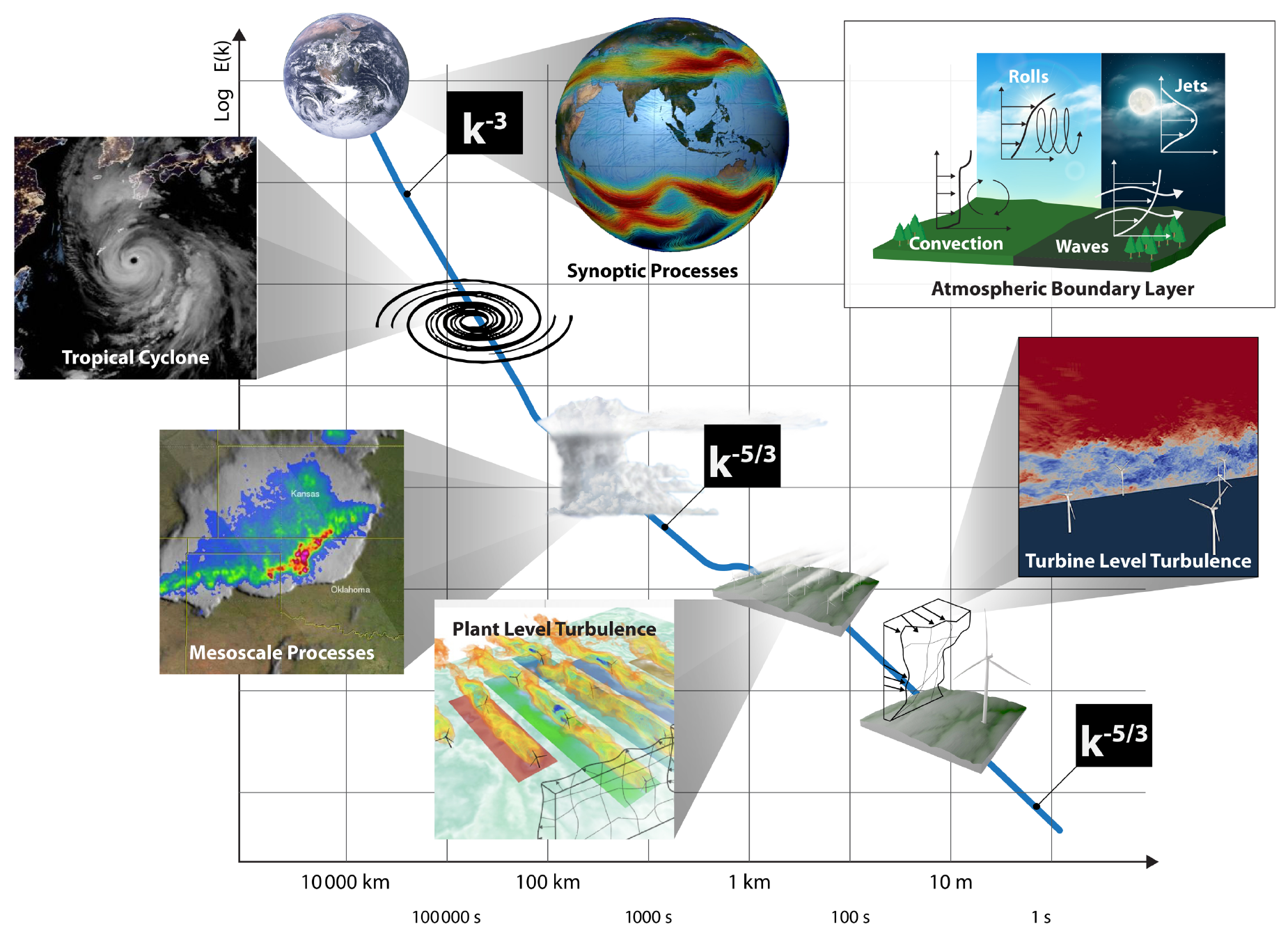
Figure 1 The cascade of kinetic energy in the atmosphere. The three main scaling regions include the largest scales, synoptic atmospheric scales with a k⁻³ spectral slope; the mesoscale range, with $k^{-\mathrm{5}/\mathrm{3}}$ slope; and small atmospheric scales with an inertial range and $k^{-\mathrm{5}/\mathrm{3}}$ slope.

While we primarily focus on the effects of atmospheric turbulence on wind turbine and wind farm performance, we also address the impact of larger-scale atmospheric motions related to extreme events that affect the characteristics of ABL turbulence that impact wind farms. The jet stream, as an example of a large-scale atmospheric phenomenon, is potentially a significant wind resource (Archer and Caldeira, 2009); however, in addition to challenges presented by harvesting high-altitude wind, extractable energy may be limited (Miller et al., 2011). Significant wind energy is associated with synoptic-scale tropical cyclones, including hurricanes and typhoons. However, these large rapidly rotating storm systems can result in surface winds significantly exceeding wind turbine design wind speeds. Hurricanes or typhoons frequently spawn mesoscale supercells, i.e., rotating thunderstorms that can create tornadoes. While tornadoes most frequently occur in North America, they are observed worldwide. Tornadoes are characterized by an extreme low-pressure funnel core surrounded by an eyewall where wind speeds can exceed 180 km h⁻¹ and reach up to 300 km h⁻¹ and, therefore, could exceed wind turbine survival wind speed. Thunderstorms can also cause damaging downburst winds (e.g., Nguyen et al., 2013). Downslope wind storms are another mesoscale process that results in strong winds, breaking waves, and increased turbulence intensity (Pehar et al., 2019). Mesoscale convective circulations and associated cloud streets, frequently observed during cold-air outbreaks over warmer bodies of water, span a range of scales from turbulent boundary layer updrafts to tens of kilometers-wide convective cells and helical rolls extending hundreds of kilometers. Large convective structures bridge the gap between atmospheric boundary layer and mesoscale motions. Consequently, the distinct separation between these scales (the “spectral gap” identified by Van der Hoven, 1957) disappears. The resulting interactions underscore the need for a more holistic approach to accurately assess the impacts of atmospheric flows on wind turbine performance and design.

3 Atmospheric boundary layers

Through contact with Earth’s surface, atmospheric flow is impacted by surface forcings: surface drag, heating or cooling, evaporation, and transpiration. Surface forcings in the form of shear and buoyancy result in turbulent flow that characterizes the atmospheric boundary layer. Turbulent eddies in the ABL range in size from energetic eddies spanning a few kilometers, i.e., the depth of the boundary layer, to millimeter-scale eddies where energy is dissipated. ABL turbulence does not evolve in isolation from the rest of the atmosphere, but instead, it is modulated by a range of scales of atmospheric motions and phenomena.

The main drivers of flows in the atmosphere, including the ABL, are large-scale pressure gradients, the apparent Coriolis force, surface heating or cooling, advection, terrain effects, and surface heterogeneities. ABL evolution over land typically follows a diurnal cycle due to differences in radiative transfer characteristics during daytime and nighttime. While the diurnal cycle is more pronounced over land than over water in coastal environments, it drives sea and land breezes. In polar regions, however, the diurnal cycle is absent or weak. The diurnal cycle over land is generally characterized by the surface absorbing and releasing heat at a significantly faster rate than the thermal response observed in the overlying atmosphere. The resulting temperature differences between the Earth's surface and the atmosphere result in unstable (convective) daytime and stable nighttime boundary layers (see Fig. 2). During daytime, the convective boundary layer can grow to a depth of a few kilometers. At the top of the convective boundary layer, a capping inversion develops, characterized by a strong temperature gradient defining an entrainment zone through which exchanges between the free atmosphere and the ABL are mediated. In contrast, when surface cooling happens at nighttime, convective structures collapse, and a stably stratified boundary layer develops of the order of tens or hundreds of meters. Between the capping inversion above and the stably stratified layer below, a residual daytime layer persists.

Figure 2 The diurnal cycle of the atmospheric boundary layer.

Regardless of atmospheric stability, turbulence in the ABL is created by shear, while buoyancy can produce or suppress turbulence depending on stability conditions. Under unstable conditions, when the surface is warmer than the atmosphere, buoyancy contributes to the formation of turbulent eddies. As eddies grow, they create a well-mixed layer capped by a temperature inversion. Under stable conditions, when the surface cools radiatively faster than the atmosphere or when warm air is advected over a cooler surface, buoyancy suppresses turbulence, resulting in reduced mixing and development of a stably stratified ABL. The interplay of shear and buoyancy creates a spectrum of turbulent structures, resulting in an inertial downscale cascade of kinetic energy to smaller eddies. The turbulent kinetic energy is also advected by wind and transported through space by velocity and pressure fluctuations. Ultimately, the kinetic energy is dissipated into heat at millimeter scales due to viscosity. The magnitude of shear and buoyancy depends on both local boundary layer conditions and large-scale atmospheric conditions. Wind energy applications are focused on cases when the wind speed is great enough (e.g., greater than 3 m s⁻¹ at hub height) for wind turbines to generate electricity. These cases are generally associated with significant shear production of turbulence, which impacts wind turbine power and loads.

Studies of idealized, canonical ABLs have been conducted extensively in the research community. They are defined as barotropic turbulent flows over horizontally homogeneous surfaces. In barotropic flows, density, pressure, and temperature isosurfaces coincide. In contrast, in baroclinic flows, isosurfaces of density and pressure do not coincide. Under steady geostrophic forcing, when the Coriolis force balances the large-scale pressure gradient, quasi-equilibrium canonical boundary layers develop and evolve due to heat (and possibly moisture) exchanges with the surface. This approach has helped us understand the structure of ABLs, their diurnal evolution, and the development of parameterizations in large-scale models. However, in reality, ABLs are embedded in continuously evolving large-scale atmospheric flows. Large-scale motions frequently evolve at a timescale comparable to the turbulent timescale, resulting in non-equilibrium conditions where turbulence production is not balanced by dissipation. Thus, real-world cases can have transient events that can result in more extreme turbulence levels and significantly impact turbine performance.

Several meteorological quantities are commonly used to quantify various characteristics of ABL flows. Next, we summarize a few of them to enhance the readability of this paper. A detailed description of these quantities is beyond the scope of this paper. The reader is encouraged to refer to Panofsky and Dutton (1983), Stull (1988), Arya (2001), Wyngaard (2010), and Morales et al. (2012) for details.

3.1 Mean and turbulence quantities of ABL flows

Instantaneous velocity components along the longitudinal, lateral, and vertical directions are commonly denoted by u, v, and w, respectively. In addition to velocity components, relevant thermodynamic variables, namely pressure, p; temperature, T; and water vapor mixing ratio, q, determine atmospheric stability. Using these thermodynamic variables, one can derive the virtual temperature, the potential temperature, and the virtual potential temperature. The virtual temperature, T_v, is a temperature at which the pressure and density of a dry-air parcel are equal to that of a moist-air parcel. The potential temperature, θ, is a temperature a parcel of fluid would attain when adiabatically brought to a reference pressure (e.g., standard surface pressure, usually p₀=1000 hPa), while the virtual potential temperature also accounts for the effects of water vapor.

$$\begin{array}{ll}{\displaystyle }& {\displaystyle }{T}_{\mathrm{v}}\approx T(\mathrm{1}+\mathrm{0.608}q);\mathit{\theta }=T{\left({\displaystyle \frac{p_{\mathrm{0}}}{p}}\right)}^{\frac{R}{c_p}}\\ \text{(1)}& {\displaystyle }& {\displaystyle }{\mathit{\theta }}_{\mathrm{v}}\approx \mathit{\theta }(\mathrm{1}+\mathrm{0.608}q)\end{array}$$

Here, R is the ideal gas constant, and c_p is the specific heat capacity at a constant pressure.

Ensemble mean values of a variable φ are represented by an overline, $\stackrel{\mathrm{‾}}{\mathit{\phi }}$. Since it is difficult to estimate an ensemble mean, in the wind energy community it is common practice to approximate it by a temporal, spatial, or combined spatiotemporal average. When conditions are nearly spatially homogeneous or temporally stationary, Reynolds decomposition of instantaneous values, φ, into mean and fluctuating quantities is applicable.

$$\begin{array}{}\text{(2)}& {\displaystyle }{\displaystyle }\mathit{\phi }=\stackrel{\mathrm{‾}}{\mathit{\phi }}+{\mathit{\phi }}^{\prime }\end{array}$$

The mean velocity components are $\stackrel{\mathrm{‾}}{u}$, $\stackrel{\mathrm{‾}}{v}$, and $\stackrel{\mathrm{‾}}{w}$, and the mean potential temperature is $\stackrel{\mathrm{‾}}{\mathit{\theta }}$.¹ The mean horizontal wind speed is $U=\sqrt{{\stackrel{\mathrm{‾}}{u}}^{\mathrm{2}}+{\stackrel{\mathrm{‾}}{v}}^{\mathrm{2}}}$. Henceforth, the mean wind speed at hub height is denoted as U_H.

Reynolds decomposition is commonly used to define turbulence quantities, including turbulent kinetic energy and turbulent fluxes of momentum and heat. The three components of velocity variances are denoted as ${\mathit{\sigma }}_u^{\mathrm{2}}$, ${\mathit{\sigma }}_v^{\mathrm{2}}$, and ${\mathit{\sigma }}_w^{\mathrm{2}}$. Turbulence kinetic energy (TKE; $\stackrel{\mathrm{‾}}{e}$) is computed as

$$\begin{array}{}\text{(3)}& {\displaystyle }{\displaystyle }\stackrel{\mathrm{‾}}{e}={\displaystyle \frac{\mathrm{1}}{\mathrm{2}}}\left({\mathit{\sigma }}_u^{\mathrm{2}}+{\mathit{\sigma }}_v^{\mathrm{2}}+{\mathit{\sigma }}_w^{\mathrm{2}}\right).\end{array}$$

Turbulence intensity is more commonly used in the engineering community. It is frequently defined along the streamwise direction: $I={\mathit{\sigma }}_u/U$. The covariances $\stackrel{\mathrm{‾}}{u^{\prime }{w}^{\prime }}$, $\stackrel{\mathrm{‾}}{v^{\prime }{w}^{\prime }}$, and $\stackrel{\mathrm{‾}}{u^{\prime }{v}^{\prime }}$ represent the components of momentum fluxes (closely related to Reynolds stress components); the sensible heat fluxes are denoted by $\stackrel{\mathrm{‾}}{u^{\prime }{\mathit{\theta }}^{\prime }},\stackrel{\mathrm{‾}}{v^{\prime }{\mathit{\theta }}^{\prime }},$ and $\stackrel{\mathrm{‾}}{w^{\prime }{\mathit{\theta }}^{\prime }}$.

Flow conditions are frequently not stationary or homogeneous. Multiresolution decomposition was developed for such conditions (e.g., Treviño and Andreas, 1996; Howell and Mahrt, 1997). Turbulence characterization under non-stationary and non-homogeneous conditions is challenging and requires careful consideration. It is currently a very active area of research (e.g., Lehner and Rotach, 2023; Arias-Arana et al., 2024).

The ABL stability results from the interplay of turbulence production and suppression. As mentioned, while shear results in production of turbulence, buoyancy can be either a source or a sink of turbulence. A non-dimensional parameter that characterizes atmospheric stability is the flux Richardson number (Ri_f), defined as the ratio of buoyancy to shear production of turbulence:

$$\begin{array}{}\text{(4)}& {\displaystyle }{\displaystyle }{\mathit{Ri}}_f={\displaystyle \frac{\frac{g}{T_{\mathrm{0}}}\stackrel{\mathrm{‾}}{w^{\prime }{\mathit{\theta }}^{\prime }}}{\stackrel{\mathrm{‾}}{u^{\prime }{w}^{\prime }}\frac{\partial \stackrel{\mathrm{‾}}{u}}{\partial z}+\stackrel{\mathrm{‾}}{v^{\prime }{w}^{\prime }}\frac{\partial \stackrel{\mathrm{‾}}{v}}{\partial z}}}.\end{array}$$

Estimating atmospheric stability using the flux Richardson number requires flux measurements, which are frequently not available. Generally, measurements of wind and temperature profiles are more readily available. An alternative non-dimensional stability parameter can be more practically estimated as a ratio of static stability (N) and wind shear (S). They can be computed as follows:

$$\begin{array}{}\text{(5a)}& {\displaystyle }& {\displaystyle }N=\sqrt{{\displaystyle \frac{g}{{\stackrel{\mathrm{‾}}{\mathit{\theta }}}_{\circ }}}\left({\displaystyle \frac{\partial \stackrel{\mathrm{‾}}{\mathit{\theta }}}{\partial z}}\right)},\text{(5b)}& {\displaystyle }& {\displaystyle }S=\sqrt{{\left({\displaystyle \frac{\partial \stackrel{\mathrm{‾}}{u}}{\partial z}}\right)}^{\mathrm{2}}+{\left({\displaystyle \frac{\partial \stackrel{\mathrm{‾}}{v}}{\partial z}}\right)}^{\mathrm{2}}}.\end{array}$$

In the atmospheric science literature, N is the Brünt–Väisäla frequency. The gradient Richardson number (Ri_g) is defined as

$$\begin{array}{}\text{(6)}& {\displaystyle }{\displaystyle }{\mathit{Ri}}_{\mathrm{g}}={\displaystyle \frac{N^{\mathrm{2}}}{S^{\mathrm{2}}}}.\end{array}$$

It can quantify the relative importance of shear production and buoyancy production/suppression. When Ri_g≈0, the atmospheric layer is considered near neutral. Positive (negative) values of Ri_g signify stable (unstable) conditions. It is generally accepted that the boundary layer flow is quasi-laminar when Ri_g exceeds unity.

Given the sparsity and generally coarse vertical resolution of profile measurements, estimating the vertical gradients of meteorological variables in a field experimental setting is challenging. As a viable alternative, one can approximate the vertical gradient of any variable χ as $\partial \mathit{\chi }/\partial z\approx \mathrm{\Delta }\mathit{\chi }/\mathrm{\Delta }z$. Thus, a widely accepted bulk parameterization for the Richardson number is defined as follows:

$$\begin{array}{}\text{(7)}& {\displaystyle }{\displaystyle }{\mathit{Ri}}_{\mathrm{B}}=\left({\displaystyle \frac{g}{{\mathit{\theta }}_{\mathrm{0}}}}\right){\displaystyle \frac{\mathrm{\Delta }\stackrel{\mathrm{‾}}{\mathit{\theta }}\mathrm{\Delta }z}{{\left(\mathrm{\Delta }\stackrel{\mathrm{‾}}{u}\right)}^{\mathrm{2}}+{\left(\mathrm{\Delta }\stackrel{\mathrm{‾}}{v}\right)}^{\mathrm{2}}}}.\end{array}$$

If the lower level of the gradient is assumed to be at the surface (z≈0), one can further simplify Eq. (7) as

$$\begin{array}{}\text{(8)}& {\displaystyle }{\displaystyle }{\mathit{Ri}}_{\text{Bs}}=\left({\displaystyle \frac{g}{{\mathit{\theta }}_{\mathrm{0}}}}\right){\displaystyle \frac{\left(\stackrel{\mathrm{‾}}{\mathit{\theta }}-{\mathrm{\Theta }}_{\mathrm{s}}\right)z}{\left({\stackrel{\mathrm{‾}}{u}}^{\mathrm{2}}+{\stackrel{\mathrm{‾}}{v}}^{\mathrm{2}}\right)}},\end{array}$$

where θ₀ and Θ_s denote reference and surface potential temperatures, respectively. It is further assumed that the wind speed vanishes at the surface. The numerator of Ri_Bs contains the term $\left(\stackrel{\mathrm{‾}}{\mathit{\theta }}-{\mathrm{\Theta }}_{\mathrm{s}}\right)$, which represents the (potential) temperature difference between air ($\stackrel{\mathrm{‾}}{\mathit{\theta }}$) and the underlying land or sea surface (Θ_s); it is commonly called air-surface temperature difference or ASTD. With weak-to-moderate wind speeds, positive (negative) ASTD leads to stable (unstable) conditions.

Under unstable conditions, both shear and buoyancy effects cause turbulent mixing. In contrast, turbulence is generated by shear and suppressed by (negative) buoyancy in stable conditions. This competition leads to significantly reduced turbulent mixing under stable conditions. In fact, under very stable (strongly stratified) conditions, the flow tends to become quasi-laminar, and turbulence can become globally intermittent, as will be discussed later.

Another parameter that characterizes an ABL is its height. While there is no single definition of the boundary layer height, it is commonly defined as a level above the surface where either TKE drops below some threshold or, alternatively, a level where the potential temperature gradient exceeds a certain value and forms a capping inversion. In the literature, the heights of the low-level jets are also used as surrogates of stable boundary layer heights. The height of the stable ABL is commonly denoted with h, while the convective, mixed-layer height is frequently denoted with z_i. Under strong convective conditions, a well-mixed boundary layer height can exceed 3 km, while under stably stratified conditions with wind speeds greater than 3 m s⁻¹ (when wind turbines produce power), a boundary layer height can be as low as several tens of meters, i.e., below the hub height of a modern utility scale with a turbine. To characterize the wind turbine operating environment under stably stratified conditions, the boundary layer height must be taken into consideration. While the boundary layer height can be inferred from remote sensing observations, direct observations are generally not available. This represents a challenge when estimating turbulence impacts on wind turbine performance since the wind shear and the turbulence level impacting turbine blades can vary significantly through a rotor rotation depending on the ABL height. Puccioni et al. (2024) used observations with a scanning lidar from the American Wake Experiment (AWAKEN) field campaign to assess ABL height. In a simulation study, Park et al. (2014) documented the influence of low-level jet heights on wind shear and turbulence intensity and, in turn, how these variables affect various turbine loads.

As an alternative to Ri_g and Ri_B (or Ri_Bs), atmospheric stability near the surface can also be quantified by the ratio $z/L$, where L is called the Obukhov length (Obukhov, 1946, 1971). The Obukhov length includes the ratio of the third power of the surface friction velocity computed from the turbulent momentum fluxes at the surface, $u_{*}=({\stackrel{\mathrm{‾}}{u^{\prime }{w}^{\prime }}}_{\mathrm{s}}^{\mathrm{2}}+{\stackrel{\mathrm{‾}}{v^{\prime }{w}^{\prime }}}_{\mathrm{s}}^{\mathrm{2}}{)}^{\frac{\mathrm{1}}{\mathrm{4}}}$, and the surface heat flux, ${\stackrel{\mathrm{‾}}{w^{\prime }{\mathit{\theta }}_{\mathrm{v}}^{\prime }}}_{\mathrm{s}}$.

$$\begin{array}{}\text{(9)}& {\displaystyle }{\displaystyle }L=-{\displaystyle \frac{{\mathit{\theta }}_{\mathrm{0}}}{g}}{\displaystyle \frac{u_{*}^{\mathrm{3}}}{\stackrel{\mathrm{‾}}{w^{\prime }{\mathit{\theta }}_{\mathrm{v}}^{\prime }}}}\end{array}$$

In convective ABLs, the absolute value of L is defined as the height above which buoyancy effects begin to dominate over the shear effects. Under neutral conditions, $z/L=\mathrm{0}$; for stable conditions, $z/L$ is positive, and for unstable conditions, $z/L$ is negative. While $z/L$ defines surface layer stability conditions, an ABL stability can be assessed using its boundary layer (or mixed-layer height) through a non-dimensional parameter $h/L$ or $z_i/L$ for convective boundary layers.

Direct measurement of L requires advanced instrumentation (e.g., sonic anemometers, scintillometers), which are rarely available within or close to wind farms, especially at offshore locations. However, the estimation of Ri_Bs only requires measurements of mean meteorological variables at a single elevation and an estimate of surface temperature. Thus, in many field studies, Ri_Bs has been computed from observed data, and in turn, L has been indirectly inferred utilizing empirical relationships proposed by Grachev and Fairall (1997) and others. The intrinsic limitations of this indirect approach have been discussed in the literature by Argyle and Watson (2014) and others. For stable boundary layers, the bulk Richardson number computed based on temperature difference between the surface and the boundary layer top is a function of a stability parameter $h/L$ (Basu et al., 2014).

3.2 Whither neutral conditions?

Contemporary turbine design standards assume inflow turbulence to be neutrally stratified (i.e., Ri_g≈0, $z/L\approx \mathrm{0}$), but neutral conditions are relatively rare in the atmosphere. In the atmosphere, exact neutral stratification (i.e., Ri_g=0, $z/L=\mathrm{0}$) is mainly associated with the transition between convective conditions and stable stratification, although near-neutral conditions can arise under several scenarios: (a) very windy conditions (i.e., shear generation completely dominates over buoyancy effects), (b) sometimes under cloudy conditions (Oke, 1987; Petersen et al., 1998), and (c) when ASTD is approximately equal to 0 (i.e., virtually negligible buoyancy effects). Over land, this last scenario persists for brief periods during morning and evening transitions (around sunrise and sunset, respectively). Haupt et al. (2019) analyzed observational data from Lubbock, Texas. They reported stable and unstable conditions to dominate at this site (see Fig. 3a). Near-neutral conditions are also infrequent offshore, as indicated by the frequency of Ri_B near zero (see Fig. 3b and c).

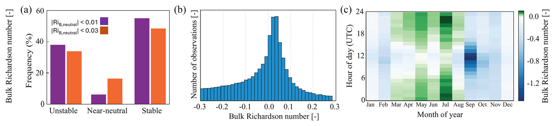
Figure 3 (a) Histograms of unstable, near-neutral, and stable conditions at the SWiFT facility, Lubbock, Texas, for 730 d between 2012–2014. The histogram shows that stable and unstable conditions are dominant at this site, while neutral conditions are not common (source: Haupt et al., 2019, ©, 1 December 2019, American Meteorological Society (AMS)). (b) Histogram of bulk Richardson number (Ri_B) calculated in the atmospheric layer between 21–90 m. (c) Diurnal and seasonal variation in (median) Ri_B indicates a pronounced seasonal cycle. During spring and summer, stable conditions are prevalent, whereas unstable conditions dominate during autumn and winter (source: Kalverla et al., 2017, published under CC BY 3.0 license). Observational data from the IJmuiden tower over the North Sea (85 km from the Dutch coastline) were utilized for the analyses in panels (b) and (c).

3.3 Wind speed and direction profiles

Mean wind speed profiles in the ABL exhibit a wide variety of shapes. Sometimes, the profile is approximately logarithmic in nature, while at other times, it can take on significantly different forms. Under certain meteorological conditions, e.g., convective or well-mixed conditions, wind speeds can be relatively uniform with height above the surface layer. Alternately, stable stratification promotes “jet” shapes with low-level wind maxima (discussed later in detail). Some of these shapes can be seen in Fig. 4a–f.

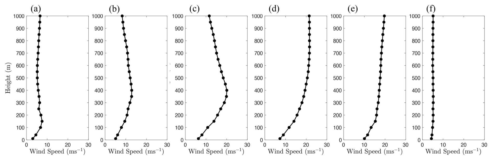
Figure 4 (a–f) Diverse wind speed profiles observed at Høvsøre, Denmark, during the Tall-Wind Profile experiment (based on the data from Peña et al., 2014).

The wind industry commonly uses a power law to represent ABL for heights across the rotor:

$$\begin{array}{}\text{(10)}& {\displaystyle }{\displaystyle }{U}_z=U_{\mathrm{H}}{\left({\displaystyle \frac{z}{z_{\mathrm{H}}}}\right)}^{\mathit{\alpha }},\end{array}$$

where U_z is the estimated wind speed at height z, and z_H is the hub height. α is the so-called shear exponent or the Hellman exponent. It is well established in the literature that α strongly varies with atmospheric stability and surface roughness (e.g., Frost, 1947; Sisterson and Frenzen, 1978; Irwin, 1979; Storm and Basu, 2010). Thus, α is expected to exhibit diurnal, seasonal, and inter-annual variations. Using observations from tall towers over the United States (US) Great Plains, Schwartz and Elliott (2006) found that α values are substantially larger at night and smaller during the day. The value of α may also depend on advection and non-equilibrium conditions, which are common in the coastal zones. Although the sum over power law functions with different exponents does not mathematically lead back to a power law function, constant values of α are often used in wind energy projects, with $\mathit{\alpha }=\mathrm{1}/\mathrm{7}(\approx \mathrm{0.14})$ and 0.2 being the most commonly used values in wind energy applications.

Wind directional shear (also called veer) is commonly estimated as

$$\begin{array}{}\text{(11)}& {\displaystyle }{\displaystyle }\mathit{\beta }=d\left(z\right)-d\left(z_r\right),\end{array}$$

where d(z) and d(z_r) are wind turning angles at heights z and z_r, respectively. During convective conditions, β is typically minimal within the entire boundary layer. However, at night, when the atmosphere is stable, average turning angles of up to 40° (between 20–200 m) have been reported (van Ulden and Holtslag, 1985; Lindvall and Svensson, 2019).

3.4 Velocity variance and TKE profiles

Turbulence in the ABL is usually generated at the surface and transported upwards. In this scenario, velocity variances and TKE monotonically decrease with height (Fig. 5a). Turbulence is also generated by shear at the inversion capping convective ABL and supporting entrainment of potentially warmer air from the free troposphere. On occasion, turbulent kinetic energy (TKE) is generated at higher altitudes by meteorological phenomena such as low-level jets or breaking gravity waves such as Kelvin–Helmholtz waves (e.g., Blumen et al., 2001) and then transported toward the ground (as shown in Fig. 5a). Such boundary layers are commonly known as upside-down boundary layers.

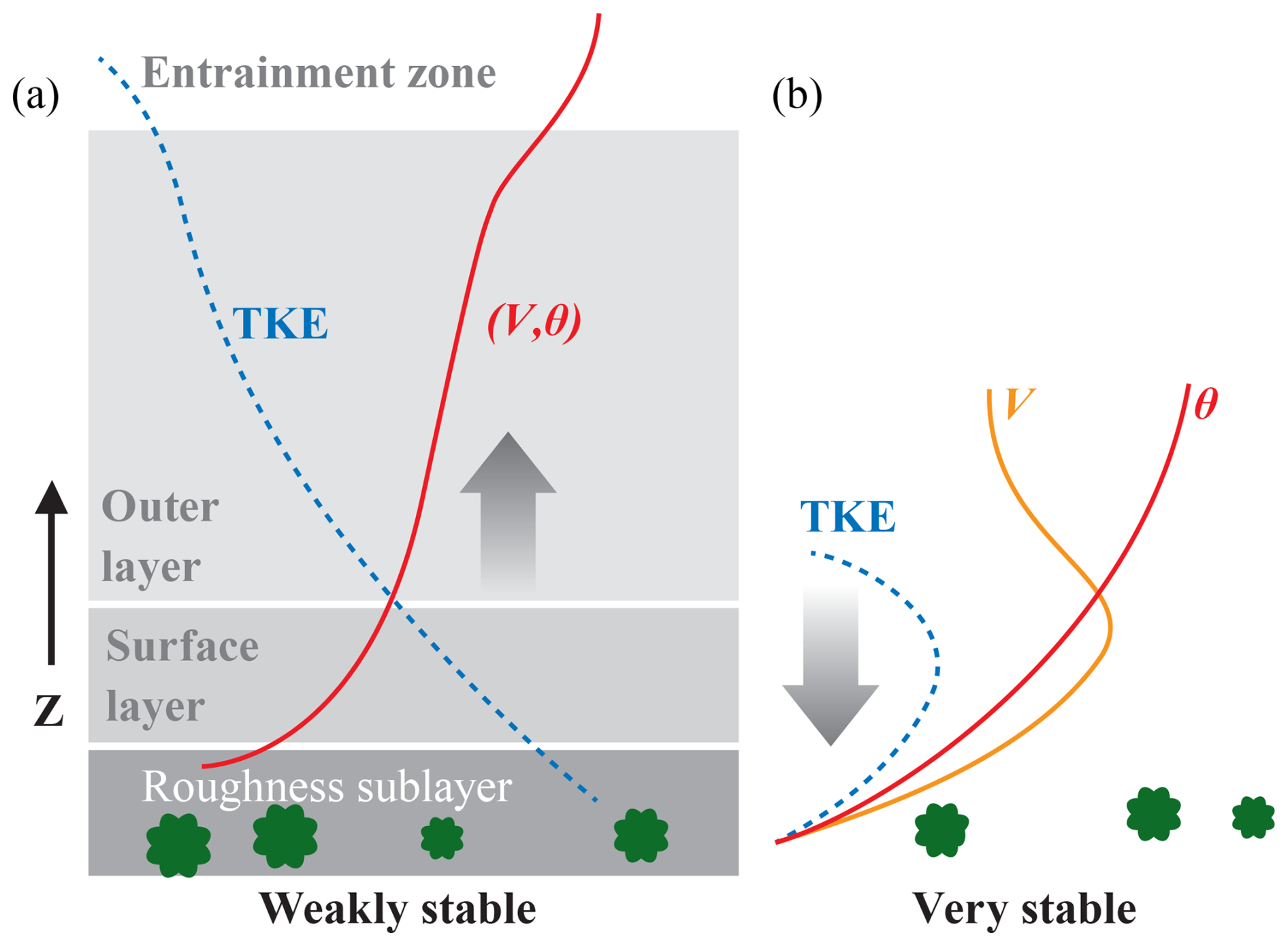
Figure 5 Schematic of TKE profiles (and other meteorological variables) in (a) weakly stable and (b) very stable conditions. A roughness sublayer is affected by surface roughness elements. A surface layer is a layer throughout which turbulent fluxes of momentum, heat, moisture, and other constituents are approximately constant, while the outer layer represents the rest of an ABL extending to the entrainment zone through which an ABL interacts with the upper troposphere (used with permission of Annual Reviews, from the Annual Review of Fluid Mechanics, “Stably Stratified Atmospheric Boundary Layers”, Larry Mahrt, 2014, permission conveyed through the Copyright Clearance Center, Inc.).

3.5 Integral length scales

The spatial dimensions of the most energetic eddies are commonly quantified by integral length scales (ILSs). ILSs are commonly estimated using correlation functions. A spatial autocorrelation function for a turbulent quantity φ is defined as

$$\begin{array}{}\text{(12)}& {\displaystyle }{\displaystyle }{\mathit{\rho }}_{\mathit{\phi }\mathit{\phi }}(\mathit{x},r{\mathit{e}}_{\mathit{\alpha }})={\displaystyle \frac{\stackrel{\mathrm{‾}}{{\mathit{\phi }}^{\prime }\left(\mathit{x}\right){\mathit{\phi }}^{\prime }(\mathit{x}+r{\mathit{e}}_{\mathit{\alpha }})}}{\stackrel{\mathrm{‾}}{{\mathit{\varphi }}^{\prime }(\mathit{x}{)}^{\mathrm{2}}}}}.\end{array}$$

Here, ρ is a spatial correlation function of a variable φ at a point in space x, r is the distance from x along the direction of the unit vector e_α, and the overline denotes the ensemble average. In the case of spatially homogeneous flows, the ensemble average can be replaced with the spatial average, while in the case of statistically stationary flows, it can be replaced with the time average. The ILS of a variable φ along the direction α is then defined as

$$\begin{array}{}\text{(13)}& {\displaystyle }{\displaystyle }{L}_{\mathit{\phi }}^{\mathit{\alpha }}=\underset{\mathrm{0}}{\overset{\mathrm{\infty }}{\int }}{\mathit{\rho }}_{\mathit{\phi }\mathit{\phi }}(\mathit{x},r{\mathit{e}}_{\mathit{\alpha }})\mathrm{d}r.\end{array}$$

If we introduce a time offset ϑ instead of the separation vector re_α, then we can compute the temporal autocorrelation and the corresponding integral timescale. An ILS determines the length beyond which the signals become uncorrelated or noise-like, which is a problematic issue in atmospheric turbulence due to the presence of larger structures. There are nine velocity ILS components corresponding to three velocity components (φ=u, v, or w) along the three spatial coordinates (α=x, y, or z). There is currently a lack of direct measurements of all autocorrelations required to estimate the individual ILS components, which limits our understanding of the ABL structure. In a review paper, Counihan (1975) reported that the ILS related to the longitudinal velocity component (i.e., u) increases with height in the lower part of the ABL. This trend is expected, as turbulent eddies typically grow larger with increasing distance from the surface. The ILS values are expected to decrease as stability increases, from unstable to neutral and then to stable conditions (for an insightful schematic, see Fig. 2 of van de Wiel et al., 2008). Based on a thorough analysis of observational data from Kansas, Kaimal (1973) reported that the integral scales (normalized with respect to height) are, in fact, inversely proportional to the gradient Richardson number. Recently, Nandi and Yeo (2021) reported ILS values for neutral boundary layers based on large-eddy simulation (LES) (see Fig. 6). While it is clear that various ILS components vary with height, determining how they vary based on observations is challenging due to the sparsity of required observations. Salesky et al. (2013) have analyzed buoyancy effects on ILS in a surface layer using observations from the HATS field study (Horst et al., 2004), while Alcayaga et al. (2022) studied coherent structures, their anisotropy, and related ILSs at 50 and 200 m under a range of atmospheric stability conditions by combining analysis of observations with a dual scanning lidar system and sonic anemometers. The analysis by Alcayaga et al. (2022) demonstrates that ILSs become more isotropic under convective conditions and further from the surface. Syed et al. (2023) conducted an analysis of longitudinal and vertical ILSs near large offshore wind farms based on aircraft observations between 100 and 250 m above mean sea level under stably stratified atmospheric conditions. They identified strong correspondence between the vertical ILS and the length scale of the vertical entrainment over a wind farm.

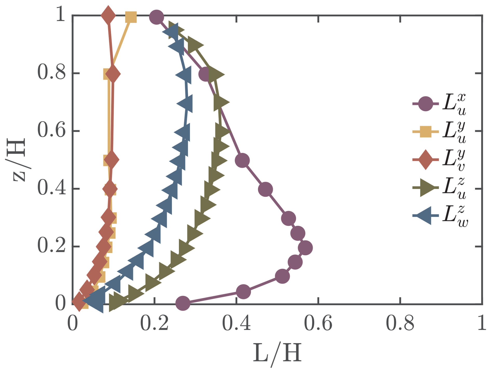
Figure 6 Integral length scales in a simulated neutral boundary layer, where H denotes the height of the boundary layer (based on the data used in Fig. 17 from Nandi and Yeo, 2021).

Fuchs et al. (2022) provide an open-source collection of different methods for estimating ILSs. However, determining all the ILS components is challenging due to the sparsity of the data. Considering these challenges, a different way to estimate relevant turbulence length scales would be beneficial. LES can provide the data needed to estimate all the integral length scales. Stanislawski et al. (2023) used LES of daytime ABLs under different atmospheric stability conditions to study the effect of turbulent inflow ILSs on wind turbine loads. They found that loads increase with increasing length scales. Hodgson et al. (2025) analyzed LESs of a flow through a wind turbine array and concluded that the power output of a wind farm depends on the ILSs of the turbulent inflow.

3.6 Statistical hierarchy, spectra, and coherence

The chaotic nature of turbulent flows makes flow variables suitable for analysis using statistical tools. The properties of the fluctuations of an observed turbulent flow scalar quantity q can be represented by the probability density function (pdf) p(q). If we consider a data set $\mathit{\{}{q}_i;i=\mathrm{1},\mathrm{\dots },N\mathit{\}}$, a pdf p(q) is insensitive to any order in the sequence i (here i can denote a time or space index). The characterization by the pdf, p(q), is complete only if two values, q_i and q_j, with $j=i+\mathrm{\Delta }$, are statistically independent. While a pdf of a flow quantity in a non-fluctuating laminar flow is represented by a delta function $p\left(q\right)=\mathit{\delta }(q-\stackrel{\mathrm{‾}}{q})$, the pdf of a turbulent flow quantity determines all its statistical moments $\stackrel{\mathrm{‾}}{q^n}=\int q^{n}p\left(q\right)\mathrm{d}q$. Statistical analysis of a turbulent flow quantity is commonly focused on central moments computed with respect to the mean value $\stackrel{\mathrm{‾}}{q}$, $\stackrel{\mathrm{‾}}{{\mathit{\mu }}^n}=\int {\mathit{\mu }}^{n}p\left(\mathit{\mu }\right)\mathrm{d}\mathit{\mu }$, where $\mathit{\mu }=q-\stackrel{\mathrm{‾}}{q}$. The second moment or variance is ${\mathit{\sigma }}_{\mathit{\mu }}^{\mathrm{2}}=\stackrel{\mathrm{‾}}{{\mathit{\mu }}^{\mathrm{2}}}$. We can define a transformed variable $\stackrel{\mathrm{̃}}{q}=\frac{\mathit{\mu }}{{\mathit{\sigma }}_{\mathit{\mu }}}$, and the associated pdf is then $p\left(\stackrel{\mathrm{̃}}{q}\right)$. In Fig. 7a, an example of $p\left(\stackrel{\mathrm{̃}}{q}\right)$, where $\stackrel{\mathrm{̃}}{q}=u^{\prime }$, is shown, in which the pdf has pronounced heavy tails. The corresponding Gaussian pdf is completely defined by $\stackrel{\mathrm{‾}}{u}=\mathrm{0}$ and σ_μ and is displayed as a solid curve. Note the large difference in the probability of large events: a μ=5σ event is more than 100 times more frequent in the empirical pdf than in a Gaussian distribution. Similarly, the pdf of normalized time increments, $\frac{\mathit{\delta }u}{{\mathit{\sigma }}_{\mathit{\delta }u}}=\frac{u(t+\mathrm{\Delta }t)-u\left(t\right)}{{\mathit{\sigma }}_{\mathit{\delta }u}}$ of velocity, has heavy tails (Fig. 7b). Quantities characterized by such heavy-tailed pdf's are also called intermittent.

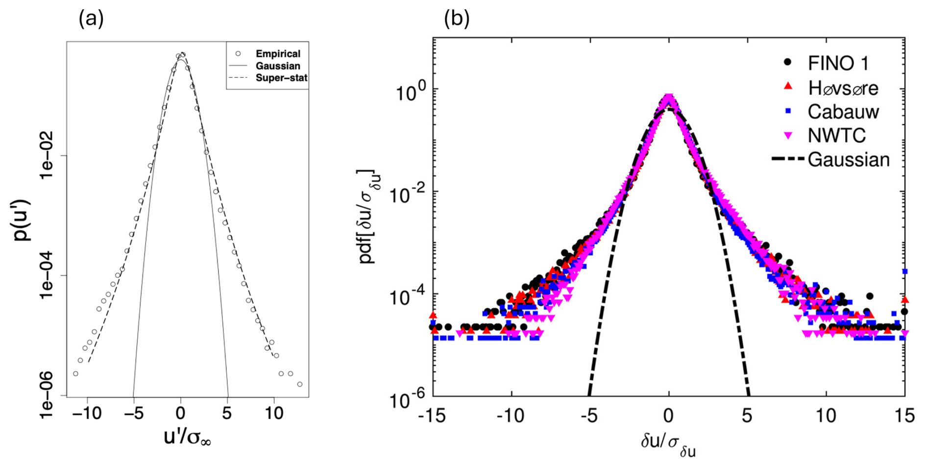
Figure 7 A pdf of fluctuating velocities from FINO1 data of January 2006. The fluctuating quantity μ is given as u^′ in units of standard deviation (Fig. 2b in Morales et al. (2012), reprinted by permission from John Wiley and Sons, © 2011 John Wiley and Sons, Ltd.). (b) A pdf of wind ramps, i.e., time increments, δu, from four tall-tower sites (FINO1, Høvsøre, Cabauw, and the National Wind Technology Center (NWTC)). Multiyear 10 min averaged wind data measured by the topmost sensors on these towers are used here (source: DeMarco and Basu, 2018, licensed under CC BY 4.0 license).

Since turbulent structures lead to dependencies of q_i and q_j, such dependencies or correlations are of interest. Statistically, this is captured by the joint pdf $p(q_i,q_j)=p(q_i,q_{i+\mathrm{\Delta }})$, which for homogeneous data depends only on the separation Δ. The lowest-order moment of this joint pdf is autocovariance $\stackrel{\mathrm{‾}}{q_i{q}_j}$. The Wiener–Khintchine theorem states that the power spectrum S_qq(n) is the Fourier transformation of autocovariance, where wavenumber or frequency, n, is proportional to $\mathrm{1}/\mathrm{\Delta }$. While a power spectrum characterizes energy content at different spatial or temporal scales, it does not characterize small-scale intermittency of turbulence. The intermittency is characterized by higher-order moments of increments $\stackrel{\mathrm{‾}}{(q_{i+\mathrm{\Delta }}-q_i{)}^n}$ (Frisch, 1995, for more details, see also Morales et al., 2012). This statistical intermittency must be distinguished from the global intermittency induced by large coherent structures such as, for example, Kelvin–Helmholtz billows.

The joint pdf can be defined for two or more variables, the so-called multivariate statistics. The moments of the different orders of multivariate joint pdf's are covariances. A covariance of two variables, q_i and r_j, is denoted by $\stackrel{\mathrm{‾}}{q_i{r}_j}$, and the corresponding Fourier transform is a complex function, the cross-spectrum $S_{qr}=C_{qr}\left(n\right)+i{Q}_{qr}\left(n\right)$, where the real part, C_qr(n), is the cospectrum, and the imaginary part, Q_rs, is the quadrature spectrum. The coherence function is defined as

$$\begin{array}{}\text{(14)}& {\displaystyle }{\displaystyle }{\text{Coh}}_{qr}\left(n\right)={\displaystyle \frac{\left|S_{qr}\right(n){|}^{\mathrm{2}}}{S_{qq}\left(n\right)S_{rr}\left(n\right)}}.\end{array}$$

Coherence can be decomposed into real and imaginary components: co-coherence and quad-coherence.

Based on measurements from a flat, uniform field site in Kansas, Kaimal et al. (1972) proposed several generalized spectra and co-spectra functions for various variables using 10 min time series. These functions systematically depend on measurement height, wind speed, and stability (see also Panofsky and Dutton, 1983).

The Mann model utilizes rapid distortion theory to model the response of turbulence to shear (Mann, 1994). It provides a spectral tensor based on the principles of flow incompressibility, linearized Navier–Stokes equations, small-scale isotropy, and large-scale anisotropy. In addition to the dissipation, ϵ, the model involves three key parameters: the size of energy-containing eddies, ℓ; the spectral Kolmogorov constant, α_K; and the anisotropy parameter, Γ, to obtain one-point spectra for velocity components (u, v, and w), co-spectra, and two-point coherence.

Figure 8 shows observed longitudinal velocity spectra for nine different stability classes for offshore station FINO1 (Cheynet et al., 2018). The spectra shown can be divided into several regimes. The high-frequency range corresponds to Kolmogorov's $-\mathrm{5}/\mathrm{3}$ inertial subrange, followed by the shear production range, characterized by a −1 spectral slope. As noted by Cheynet et al. (2018), this −1 slope is particularly evident in the top panels, corresponding to the unstable ABL. The spectral peak represents the largest eddies in the ABL. Under stably stratified conditions (lower panels), there is a pronounced spectral gap between the mesoscale range at the lowest frequencies and the spectral peak. Studies have suggested that the gap between the latter two ranges is not always present. Larsén et al. (2016, 2018) demonstrated with measurements from the surface to about 250 m that the gap exists and can be modeled. In agreement with, e.g., Högström and Smedman-Högström (1974), Cheynet et al. (2018) showed that the gap can be deep or shallow depending on atmospheric stability. Full-scale spectral models for the wind components u and v are provided in Larsén et al. (2016, 2021). In a follow-up study, Sim et al. (2023) analyzed a 20-month-long record of high-frequency (1 Hz) observations of wind speed and examined spectra extending to low frequencies corresponding to a large atmospheric flow timescale. Their analysis confirmed previous findings based on aircraft data (e.g., Nastrom and Gage, 1985).

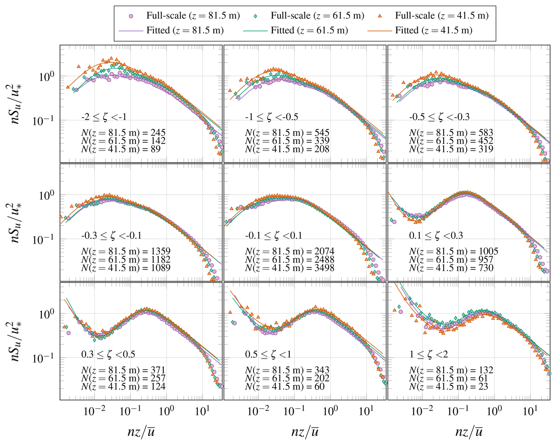
Figure 8 Longitudinal velocity spectra for nine stability regimes. The top, middle, and bottom panels represent unstable, near-neutral, and stable regimes, respectively. Observational data from the FINO1 tower, located in the North Sea, are used for spectral analysis. The variable ζ represents the so-called stability parameter, the ratio of height to local Obukhov length, and $nz/\stackrel{\mathrm{‾}}{u}$ denotes the reduced frequency of frequency n (based on Fig. 7 from Cheynet et al., 2018, courtesy of Etienne Cheynet).

Coherence for both u and v is usually parameterized in terms of frequency f (or wavenumber), wind speed U, distance Δ, and a decay coefficient a (Davenport, 1961):

$$\begin{array}{}\text{(15)}& {\displaystyle }{\displaystyle }\left|\text{Coh}\right(f,\mathrm{\Delta }\left)\right|={\mathrm{e}}^{-a\frac{f\mathrm{\Delta }}{U}}.\end{array}$$

Davenport (1962) estimated the parameter a=7 for separation in both cross-wind and vertical directions. However, further studies demonstrated that the parameter a is not constant but rather depends on the atmospheric stability (e.g., Panofsky and Mizuno, 1975). While coherence analyses based on observations focused on mean wind direction, Berg et al. (2016) demonstrated how turbulence-resolving numerical simulations can be used to analyze coherence of three velocity components. They compared simulated non-Gaussian velocities to Gaussian fields and showed that their coherences are similar. They also found that as the separation increases, the largest coherence switches from the vertical to the cross-wind component. While the longitudinal coherence is less important for a wind turbine design, it is important for the turbine control (e.g., Schlipf et al., 2013). Thedin et al. (2023) used a turbulence-resolving simulation driven by large-scale forcing derived from a mesoscale simulation to analyze coherence of three velocity components in three spatial directions and pointed out the limitation of numerical simulations that do not resolve high-frequency fluctuations. For large-scale, quasi-geostrophic turbulence, Vincent et al. (2013) analyzed coherence as a function of separation and angle with respect to a mean wind direction using observations and mesoscale simulations. They extended a form of Davenport's coherence model to large separations that represent the coherence at mesoscale.

For typical boundary layer turbulence, Panofsky and Dutton (1983) found a∼60 for u and 7 for v. For two-dimensional turbulence, Vincent et al. (2013) found a∼7.7 for u and 5 for v, suggesting significantly stronger coherence in the longitudinal wind component over time and space. The cross-stream velocity component, v, is better correlated in large-scale flow than in three-dimensional turbulence, though not as significantly as the u component.

3.7 Global intermittency and coherent structures

One of the intriguing characteristics of boundary layers is the existence of (globally) intermittent turbulent bursts and associated coherent structures (Shaw and Businger, 1985; Mahrt, 1989). These seemingly random yet highly organized (coherent) features are generated by various atmospheric processes, such as density current and internal gravity waves (Sun et al., 2004). Illustrative examples can be seen in Fig. 9. The impacts of these features on various turbine loads are discussed in the following sub-section.

Figure 9 Streamwise velocity variance measured by a lidar (adapted from Fig. 7 in Banta et al., 2008, © IOP Publishing, reproduced with permission, all rights reserved). The mean wind speed profile, depicting strong shear, is overlaid. The presence of intermittent turbulence is clearly visible. On several occasions, the turbine design thresholds are exceeded during these bursting events.

In the literature, only a handful of idealized numerical studies (e.g., Zhou and Chow, 2011; Ansorge and Mellado, 2014; He and Basu, 2015) have successfully reproduced some characteristics of observed intermittent turbulence. To the best of our knowledge, realistic simulations, such as LES or gray-zone modeling, of these flow features are still lacking. Since intermittent turbulence events are often of high amplitude but short in duration, traditional stationary or linear signal processing techniques frequently fail to detect or characterize such phenomena. To address this shortcoming, Rinker et al. (2016) developed a technique that introduces temporal coherence, which results in a non-stationary signal. Their approach may be utilized to generate turbine inflow generations using stochastic simulations.

4 Some relevant atmospheric phenomena

Low-level jets (LLJs), mesoscale convective rolls and cells, gravity waves, terrain-induced circulations, and downslope windstorms are atmospheric phenomena with distinct wind and turbulence structures. The mechanisms and characteristics of these phenomena are briefly introduced here, as their impacts on power production and loads are discussed in Sects. 7 and 8, respectively. These phenomena occur both on land and offshore. For more detailed information about offshore environments relevant to wind energy applications, see Shaw et al. (2022), which covers aspects such as the effects of ocean surface waves. As a result, specific details of offshore conditions are not extensively addressed in this paper.

4.1 Low-level jets

LLJs are fast-moving air currents within several hundred meters of the surface. They typically occur at night and are common in many areas. The North American Great Plains LLJ is a well-known example that occurs almost every night over central North America (e.g., Bonner, 1968; Zhong et al., 1996; Whiteman et al., 1997; Berg et al., 2015). LLJs are also common over central South America (e.g., Marengo et al., 2002, 2004; Gimeno et al., 2016) and many offshore and coastal areas worldwide (e.g., Winant et al., 1988; Burk and Thompson, 1996; Parish, 2000; Kalverla et al., 2019; Lima et al., 2019; Debnath et al., 2021; Aird et al., 2022; de Jong et al., 2024; Olsen et al., 2025). LLJs can be caused by various physical mechanisms, such as inertial oscillation, sloping terrain, cold fronts, baroclinicity due to land–sea temperature contrasts in coastal areas, barrier winds, and other topographically induced adjustments. Figure 10 provides examples of vertical wind profiles in onshore and coastal LLJs. The figure demonstrates that LLJs generate high-amplitude wind speeds, creating strong shear. In addition to strong shear, significant wind veer is a characteristic of LLJs (e.g., Vanderwende et al., 2015). Above the LLJ nose, the shear is negative, affecting wind turbine loads (see Sect. 8.2.1). Due to their relatively low altitude above ground level, typically 100 to 500 m (Fig. 10), LLJs have important implications for wind resource assessments, wind power forecasting, and turbine loading, particularly as wind turbines become taller and rotors bigger.

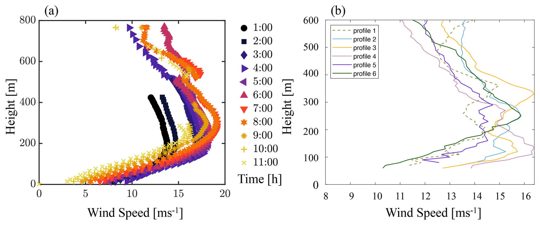
Figure 10 (a) A developing LLJ was observed in Colorado during the Lamar Low-Level Jet Project in 2003. Wind speed profiles were estimated by averaging lidar observations over an hour (based on data used in Fig. 7 from Banta, 2008). (b) Wind speed profiles showing a LLJ in the German Bight in the North Sea, from the airborne measurement data published in Bärfuss et al. (2019), on 14 October 2017 from about 13:23–16:23 LT. The corresponding flight tracks to the profiles can be found in Fig. 2 in Larsén et al. (2021), covering the area from 53.85 to 54.20 ° N and 6.95 to 7.65 ° E.

The global distribution and characteristics of onshore and coastal LLJs have been studied using global simulations and reanalysis datasets (e.g., Rife et al., 2010; Ranjha et al., 2013; Lima et al., 2018). In addition, several studies have utilized high-resolution mesoscale models to downscale global data (e.g., Soares et al., 2014, 2019; Rijo et al., 2018). However, mesoscale simulations of LLJs are challenging. Storm et al. (2009) investigated the performance of the Weather Research and Forecasting (WRF) model in simulating the North American Great Plains LLJ. They found that the WRF model, with various physical configurations, can capture some of the observed LLJ's characteristics, such as its location and timing. However, the model overestimated the LLJ height, while underestimating its strength compared to observations. Nunalee and Basu (2014) found that WRF generally underestimated the intensity of offshore LLJs. Using data collected at an Iowa wind farm during the Crop Wind Energy Experiment (CWEX) field study, Vanderwende et al. (2015) showed that the WRF-simulated LLJ properties depended on the initial and boundary conditions, as well as the employed boundary layer parameterizations. Aird et al. (2021) used WRF to study seasonal variation in LLJs over Iowa and investigated the dependence of LLJ characteristics on vertical resolution and criteria for identifying LLJs. The shortcomings of WRF in capturing LLJs highlight the need for further research to improve the representation of critical atmospheric boundary layer processes. Muñoz-Esparza et al. (2017) performed high-resolution WRF simulations using nested domains ranging from mesoscale up to LES domains to simulate the diurnal cycle dynamics of the CWEX field study. They demonstrated that LES nested in a mesoscale domain can accurately capture the magnitude of the LLJ and associated turbulence properties. This seems to suggest that the standard setup of WRF may be too coarse to resolve the atmospheric dynamics of an LLJ. Using the US Navy's COAMPS model, Ranjha et al. (2016) investigated the resolution dependence of coastal LLJs. As expected, the model produced more realistic flow features with increasing horizontal resolutions from 54 to 2 km. Interestingly, the model's performance did not show a monotonic behavior concerning spatial resolution in terms of traditional skill scores.

To accurately model LLJs, we need to improve our understanding of the phenomenon and, simultaneously, our understanding of different models' capabilities. The nature of LLJs requires a mesoscale model to resolve the large-scale atmospheric flow characteristics and a high-resolution model to resolve the small-scale turbulence. Since Lettau and Davidson (1957) first identified LLJs during the Great Plains Project, there have been many attempts to unequivocally define an LLJ (e.g., Bonner, 1968; Whiteman et al., 1997; Banta et al., 2008); however, this did not result in a generally accepted definition. Such a definition is elusive due to the relative sparsity and low resolution of observations. We need more coordinated measurement campaigns with instruments for both mesoscale and microscale flows. AWAKEN (Moriarty et al., 2024) is a field study that aims to provide such observations. In a recent analysis of long-term observations of LLJs at the Atmospheric Radiation Measurement Southern Great Plains site, Debnath et al. (2023) used the following criteria to detect LLJs: location of the wind speed maximum, where the difference between the wind speed maximum and the wind speed at the top of the jet is at least 2 m s⁻¹ and this difference exceeds 10 % of the maximum wind speed. They found that the LLJ wind profile cannot be represented by the shear exponent only.

Several attempts to analyze spectral features associated with the LLJ structure and relate them to spectra observed in canonical stably stratified ABLs without a jet (Kaimal, 1973) did not result in consistent findings. While Smedman et al. (2004) and Hallgren et al. (2022) found that low frequencies of the streamwise velocity spectra associated with LLJs are suppressed, these results are not consistent with those of other studies (e.g., Duarte et al., 2012). The knowledge gained from the further analysis of these and other measurements that include characterization of mesoscale conditions is expected to shed light on how to couple mesoscale and microscale modeling to fit the LLJ's nature.

4.2 Mesoscale convective circulations – rolls and cells

Mesoscale convective circulations accompany synoptic weather systems such as fronts or cold- and dry-air outbreaks from the continent or ice shelves over a neighboring warm surface. Significant differences in temperature and humidity between a relatively warmer sea surface and colder overlying air, combined with large wind shear, can result in helical roll vortices (LeMone, 1973). Rolls with single or multiple thermals within the roll updraft regions can lead to cloud streets (Kuettner, 1971). Observations suggest that, as the distance from the coastline increases, rolls change into three-dimensional, circular open cells with an upward motion on the edge and downwards motion in the center (Atkinson and Zhang, 1996; Young et al., 2002; Salesky et al., 2017). These organized atmospheric structures exhibit coherent updrafts and downdrafts, contributing significantly to the vertical turbulent fluxes of momentum, heat, and humidity. Consequently, they influence surface fluxes, the height of the boundary layer, and the spatial correlation of meteorological parameters such as wind, temperature, humidity, and particle concentrations. Typical characteristics of rolls and cells are summarized in, e.g., Atkinson and Zhang (1996), Etling and Brown (1993), Young et al. (2002), and Banghoff et al. (2020). Their summary suggests that rolls align along or at angles up to 10° from the mean horizontal wind, with typical lengths of 20–200 km, widths of 2–10 km, and convective depths of up to 3 km. They have been observed over both water and land surfaces. Convective cells, on the other hand, typically have diameters ranging from a few kilometers to 40 km and a convective layer depth of 1–5 km.

The need to study rolls and cells lies in the fact that they are common phenomena frequently observed over the globe, over both water and land, resulting in significant fluctuations in wind speed that impact wind power production and significant levels of turbulence that impact turbine loads. Agee (1987) showed a global distribution of the presence of convective cells. The favorable thermal and dynamical conditions that produce them can occur in connection with cold-air outbreaks and fronts (e.g., Skyllingstad and Edson, 2009; Vincent, 2010), regional flow such as mistrals and the tramontane (e.g., Brilouet et al., 2017), and hurricanes (e.g., Zhu, 2008; Worsnop et al., 2017b). They have been observed in the North Sea (e.g., Brümmer et al., 1985; Vincent, 2010), in the Mediterranean Sea (Brilouet et al., 2017), in the Yellow Sea (Chen et al., 2019), along the US Gulf Coast (Young et al., 2002), along the East Coast of the US (e.g., Fig. 11a), in Siberia, in Japan, south of the Bering Strait (Agee, 1987; Atkinson and Zhang, 1996), and over the East China Sea (Hsu and yih Sun, 1991). Most often, they were observed under near-neutral and convective conditions, though sometimes rolls were also found under stable conditions. In Svensson et al. (2017), rolls were observed over the Baltic Sea under stable conditions. These rolls were originally generated under convective conditions over land and then advected and maintained at least 30–80 km off the coast.

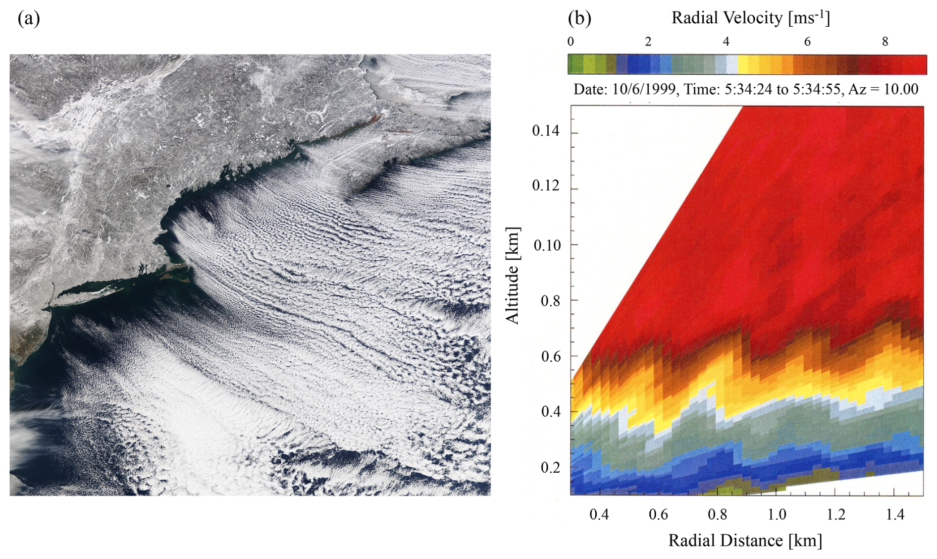
Figure 11 (a) Satellite image of clouds over the East Coast of the US, associated with a cold-air outbreak on 24 January 2011 (NASA Worldview Snapshots), indicating the presence of mesoscale convective circulations, convective rolls closer to the coast, and convective cells further downwind from the coast. (b) NOAA's wind lidar (HRDL) captured gravity waves on 6 October 1999 during the CASES-99 field campaign (source: Poulos et al., 2002, © American Meteorological Society, used with permission.).

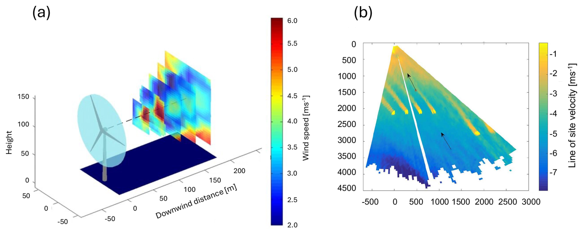
Figure 12 (a) Samples of wind speeds measured using nacelle-mounted Doppler lidar (source: Trujillo et al., 2016, published under CC BY 3.0 license). (b) A ground-based scanning lidar horizontal scan (source: Bodini et al., 2017, published under CC BY 3.0 license).

4.3 Gravity waves

In a stable atmosphere, wind flow perturbed upwards over a hill or ridge or by a strong convective updraft (e.g., thunderstorm) can experience a restoring force that can create oscillations and trigger waves to be transmitted perpendicular to the streamlines over the orographic feature. While gravity waves can occur throughout the troposphere, of relevance for wind energy are gravity waves that impact boundary layer flows. In a stably stratified ABL, gravity waves can be trapped by a strong potential temperature inversion (e.g., Fig. 11b). When the temperature stratification is sufficiently strong and the winds are moderate, i.e., when the Froude number is subcritical, $\mathit{\text{Fr}}=\frac{U}{Nh}<\mathrm{1}$ (here h is the obstacle height), the waves can be reflected back down to the ground, and such trapped atmospheric gravity waves (AGWs) are known as “lee waves” (Nappo, 2013). Lee waves can propagate long distances downstream from the orographic feature that generated them, as demonstrated by, for example, Larsén et al. (2011), and impact flow in the boundary layer. Under synoptic conditions, with a strong pressure gradient perpendicular to a mountain range, lee waves can cause downslope wind storms and result in a hydraulic jump. AGWs occur widely in the atmosphere (Mahrt, 2014; Urbancic et al., 2021), leading to wind speed variations of the order of minutes to hours, which can cause wind farm power output fluctuations. Although this scale of fluctuation does not impact turbulent loading, wind shear and wave breaking can generate turbulence, leading to what is sometimes termed an “upside-down” atmosphere with higher levels of turbulence aloft (Mahrt, 1999); see Fig. 5b.

AGWs enhance wind speed at the wave crests, which increases bulk shear instability, generating eddies that promote strong turbulent mixing from above and potentially create small LLJs; near the surface, wave troughs promote local shear, contributing to the generation of weak turbulence (Sun et al., 2015). However, the impact of AGWs on small-scale turbulence near the surface has not been studied yet.

4.4 Terrain-induced circulations

Wind farms are frequently deployed in locations where terrain effects result in favorable wind conditions. Land or sea breezes resulting from differences in surface heating rates between land and water and topographically induced circulations, such as speed-ups on ridges or escarpments, gap flows, and drainage flows, can represent a significant wind resource. However, terrain-induced circulations can also be characterized by significant wind variability and non-equilibrium turbulence that impact wind farm performance. Historically, characterization of turbulence in an ABL focused on flows over flat and primarily horizontally homogeneous terrain, while boundary layer studies in mountainous terrain concentrated on characterizing the mean structure of the mountain ABL (e.g., Whiteman, 2000). During the last few decades of the 20th century, several field studies focused on flows over isolated hills, e.g., Blashaval Hill (Mason and King, 1985) and Askervein Hill (Taylor and Teunisse, 1987), as well as transport and dispersion (Lavery et al., 1982). The Atmospheric Studies in Complex Terrain (ASCOT) was a major program focused on characterizing drainage flows and turbulent mixing (Orgill and Schreck, 1985) followed by the VTMX 2000 field study (Doran et al., 2002). Over the last few decades, several field studies have been designed to address turbulent ABLs in complex terrain and the range of processes affecting their structure. Some examples are the Mesoscale Alpine Program (MAP) Riviera project (Rotach and Zardi, 2007), which focused on a diurnal cycle of valley flows; the T-Rex project (Grubišić et al., 2008), which was a study of mountain-induced rotors; COLPEX (Price et al., 2011), which analyzed cold-pool processes; MATERHORN (Fernando et al., 2015), which addressed a combination of topography and thermally induced circulations; and the METCRAX and METCRAX II field studies (Whiteman et al., 2008; Lehner et al., 2016), which focused on stably stratified boundary layers. The early field studies were also used to validate numerical models. However, turbulence-resolving large-eddy simulations have only recently been applied to flows over complex terrain (e.g., Chow et al., 2006; Chow and Street, 2009; Babić and De Wekker, 2019; Arthur et al., 2022). Chow et al. (2019) summarized the advances and challenges in simulating and forecasting flows in complex terrain. While these field and numerical studies were not focused on wind energy applications, they represent an important resource for understanding and characterizing the conditions under which wind farms in complex topography operate. Most of the field studies conducted to date have focused on specific flow phenomena; however, the diversity of complex terrains, resulting in a variety of frequently interacting phenomena, represents a challenge to developing a systematic understanding of turbulence and its evolution in complex terrain.

Downslope windstorms develop under favorable synoptic conditions and stable stratification when a cross-mountain range flow results in gravity waves and flow acceleration near the surface on the lee side of the mountain. In downslope windstorms, wind gusts can exceed 60 m s⁻¹ (Čavlina Tomašević et al., 2022). These storms can form when the mountain top is at least 1 km above the lee-side terrain with a steep lee-side slope. A detailed review of mountain wind storms can be found in Durran (1990). Winds associated with mountain ranges that frequently result in wind storms across the world include Chinook in the Rocky Mountains, Foehn in the Alps (Haid et al., 2020), Bora wind along the eastern Adriatic (Lepri et al., 2017), Zonda wind in South America (Loredo-Souza et al., 2017), the Santa Ana and Diablo winds in California (Fovell and Cao, 2017), and Yamajikaze wind in Japan (Kusaka and Fudeyasu, 2017), to name a few.

5 Observing ABL flows

A wide range of instrumentation, including in situ and remote sensing, can be used to quantify the characteristics of mean flow and atmospheric turbulence. Over the last 50 years, sonic anemometers have been the workhorse in situ instruments in boundary layer studies (Kaimal, 1986). Sonic anemometers can measure all three components of the velocity vector and sample at high frequency so that the energy and momentum fluxes can be computed using the eddy-covariance method. When combined with independent temperature measurements, sonic anemometers can provide high-rate measurements of acoustic temperature, which represents a good approximation of a virtual temperature, which accounts for the water vapor in the air. By simultaneously measuring velocity components and virtual temperature, using the eddy-covariance method, sonic anemometers can provide sensible heat fluxes. Using measurements of momentum fluxes and sensible heat fluxes, one can estimate the Obukhov length. By assuming that turbulence is frozen in time as it advects by a sensor, i.e., using Taylor's hypothesis (see Wyngaard, 2010), one can use high-rate time series of measurements at a point in space and interpret them as a spatial record. In other applications, such as resource assessment, cup or propeller anemometers are commonly used, though their frequency response is inferior to that of sonics. With these sensors, one can compute estimates of the turbulence intensity based on the standard deviation of the wind speed over a time interval of interest. Sonic, cup, and propeller anemometers must be mounted on towers or some other support structure, meaning that they represent only a very small area and are generally located relatively close to the surface.

In situ measurements can also be made using dedicated aircraft with appropriate instruments (e.g., Schmid et al., 2014; Laursen et al., 2006). These can include crewed aircraft of various sizes, and wind is measured using a pitot tube and the craft's navigation system. Deployment of these aircraft for ABL studies is generally expensive, and past research has focused on intensive measurement campaigns and specific case studies. In addition, it is not easy to measure the time evolution of wind using an airborne platform. Recently, there has been interest in the deployment of smaller, uncrewed aircraft to measure boundary layer winds, and these systems will likely become more common in the future (Pinto et al., 2021).

Remote sensing systems have increasingly been used to address shortcomings associated with in situ measurements. Radar wind profilers are commonly used to measure profiles of wind speed and wind direction from approximately 70 m above the surface to many kilometers aloft, depending on the frequency of the radar used in the system. Scanning radar systems, such as Ka-band radar, have been used to study flow in and around wind farms (e.g., Hirth et al., 2012). Doppler sodars, which can measure profiles of wind speed and direction in the lowest several hundred meters of the atmosphere, have been used in a wide range of field studies (e.g., Wilczak et al., 2019). Recently, however, they have largely been replaced by Doppler lidar systems in many applications. Some lidar systems are configured to measure only the profile of wind speed and direction using fixed-stare directions. These lidars have also been installed on buoys and other floating platforms to provide profiles of wind speed and direction in maritime environments (e.g., Gorton and Shaw, 2020). In addition to the mean profiles, algorithms have been developed to derive TKE and TI using these systems. The field study 3D Wind, conducted over a large wind farm using in situ and remote sensing instruments, focused on the structure of wind and turbulence in a lower region of an ABL relevant for wind energy and found good agreement between lidar and cup anemometer observations (Barthelmie et al., 2014). However, differences have been observed compared with measurements from sonic anemometers (Sathe et al., 2015). Other systems are configured to scan in arbitrary patterns. They can be used to probe the nature of the flow over a larger area or can be combined to scan in a coordinated pattern to provide measurements akin to virtual towers (e.g., Newsom et al., 2013) or measurements over a relatively large area (e.g., Berg et al., 2017). Scanning lidars can also be mounted on wind turbine nacelles to investigate details of the inflow to the turbine or wakes (e.g., Borraccino et al., 2017; Trujillo et al., 2016) (Fig. 12) or used as input to turbine controls to reduce loads (e.g., Held and Mann, 2019). Field studies, such as the eXperimental Planetary boundary layer Instrumentation Assessment (XPIA), provided the opportunity to compare measurements from Doppler lidar and sonic anemometers and showed good agreement between measurements made in situ and those using lidars and radars (Lundquist et al., 2017).

There have been several recent field studies to characterize mean and turbulent flow in complex terrain with an emphasis on resource assessment and forecasting, including the Wind Forecast Improvement Project 2 (WFIP2 Shaw et al., 2019; Wilczak et al., 2019) and a series of New European Wind Atlas field studies (Mann et al., 2017): the Perdigao experiment (Fernando et al., 2019), Alaiz experiment (Santos et al., 2020), and Kassel Forested Hill experiment (Pauscher et al., 2017). These studies have produced a wealth of unique observations that will continue to provide opportunities for insightful analysis of turbulence characteristics as they may be modulated by complex terrain and thus deviate from observations in flat terrain. The challenge is to develop and demonstrate effective methodologies to estimate turbulence characteristics over heterogeneous terrain that could be used to optimize wind farm layout and turbine design. For example, Wildmann et al. (2019) used lidar range–height indicator (RHI) scans during the Perdigao experiment to retrieve the turbulence dissipation rate using the modified Doppler spectral width method validated against tethered lifting-system-based hot-wire anemometer measurements and demonstrated good agreement between remote sensing and in situ observations of dissipation. Wildmann et al. (2020) used dual-Doppler lidar observations to estimate turbulence intensity, including in the wake of a wind turbine located at the western ridge of the Perdigao field study. Peña and Santos (2021) combined scanning lidar observations and numerical simulations over a selected period during the Alaiz field study and demonstrated that it is possible to simulate an observed hydraulic jump in the lee of the Alaiz mountain. The hydraulic jump develops under strong downslope wind conditions resulting from cross-mountain flow and associated mountain waves. The effects of complex, hilly terrain on turbulence characteristics in wind farms are also studied using wind tunnel experiments (e.g., Kozmar et al., 2018). There are ongoing field studies focused on complex terrain, including at the WINSENT research facility (WindForS, 2024) and the coastal research wind farm WiValdi (Research Alliance Wind Energy, 2024).

Observations in complex terrain present several challenges. They are related to the representativeness of in situ measurements and characterization of flow and turbulence inhomogeneities and non-equilibrium effects, which need further exploration.

6 Modeling of ABL flows

High-rate, in situ atmospheric measurements of turbulence using, for example, sonic anemometers, provide the most reliable characterization of ABL turbulence (e.g., Mann et al., 2009). However, such measurements are either sparse or not always available when considering wind farm development and wind turbine siting. More often available are only estimates of turbulence intensity based on cup anemometer measurements. Numerical simulations can complement observations or be used as an alternative. However, numerical simulations of atmospheric flows are limited by computational requirements and available computational resources. Currently, simulations that resolve all the scales of atmospheric motions are impossible. Instead, three types of atmospheric simulations are employed, each resolving a different range of scales. Global circulation simulations resolve the largest scales, planetary waves, and synoptic systems with grid cell sizes down to an order of 10 km. Global weather simulations are downscaled using limited-area models to resolve regional weather: storms, mesoscale convective systems, and effects of topography and other surface heterogeneities with grid cell sizes of the order of a couple of kilometers. In global and mesoscale simulations, three-dimensional boundary layer turbulence is still fully parameterized and is not a reliable alternative to observations. Design application and estimation of turbine loads require numerical simulation of the inflow turbulence impacting a wind turbine. Ideally, multiscale simulations, including high-resolution microscale simulations, could provide realistic ABL turbulence fields; however, such simulations are computationally challenging. An alternative approach consists of rapid generation of idealized turbulent fields based on prescribed turbulence spectra.

TurbSim (Kelley and Jonkman, 2007) is one of the most commonly used tools that can rapidly generate a range of idealized turbulent fields. To meet the new design needs, TurbSim must be extended to provide a wider range of realistic turbine inflows. Turbulent inflow can also be generated using LES; however, such simulations are computationally expensive. Therefore, there is still a need for a faster alternative. In addition to a tool like TurbSim, recent developments in artificial intelligence and machine learning (AI/ML), in particular state-of-the-art physics-informed deep learning approaches, provide an opportunity to develop ML models using vision transformers that can generate realistic turbulent fields at a fraction of the cost of an LES (e.g., Stengel et al., 2020; Dettling et al., 2025). Alternatively, coupled simulations could be used to create a public database of ABL flows, similar to the Johns Hopkins Turbulence Database (Johns Hopkins University, 2021).

As larger modern turbines are exposed to a wider range of atmospheric conditions, there is a need to better represent the turbulent inflow that impacts their performance. To resolve ABL turbulence, from the largest boundary layer eddies into the inertial range of turbulence characterized by the Kolmogorov $-\mathrm{5}/\mathrm{3}$ spectrum (Kolmogorov, 1941), we can employ large-eddy simulations (LESs). High-resolution LES with properly validated numerical models can complement measurements. LES resolves large turbulent eddies extending into the inertial range. The inertial range is characterized by a forward cascade transferring kinetic turbulent energy down to small scales and is marked by the so-called $-\mathrm{5}/\mathrm{3}$ scaling. The universal scaling enables effective parameterization of the effect of small, unresolved eddies on resolved ones. Estimating the direct impact of the ABL turbulence on wind turbine power production requires resolving eddies spanning 2 to 3 orders of magnitude in size. The largest ABL eddies, in general, scale on the ABL height and are of the order of thousands of meters, while the smallest eddies impacting turbine performance are of the order of meters, corresponding to a frequency of a few hertz.

Since its inception more than 50 years ago (Lilly, 1966, 1967), LES has been effectively used to study idealized, canonical ABLs (e.g., Deardorff, 1972; Moeng, 1984; Andren, 1995; Kosović and Curry, 2000). LES has been used as a research tool to study the interaction between ABL flows and operating turbines, represented using either actuator disk models or actuator line models (Sørensen and Myken, 1992; Sørensen and Shen, 1996; Troldborg et al., 2007). Actuator disk and line approaches were initially used in idealized Reynolds-averaged Navier–Stokes (RANS) simulations that did not account for some of the complexities of canonical ABL flows, such as atmospheric stability. Due to relatively modest computational requirements, RANS simulations are still the tool of choice for design purposes, even though in these simulations, only the mean flow properties are represented, and turbulence is fully parameterized. More recently, the representation of operating turbines was implemented in atmospheric LES models, allowing for the analysis of atmospheric stability effects on wind turbine wakes (Mirocha et al., 2014; Aitken et al., 2014). High-performance computing (HPC) capabilities, including new accelerator technologies (e.g., general purpose graphical processing units or GPGPUs), enable blade-resolving LESs (Sprague et al., 2020). As the HPC approaches exascale computing, LES will become accessible for a range of applications and will not only be used as a research tool (Sanchez-Gomez et al., 2024).

Turbulence in an ABL is frequently affected and modulated by surface heterogeneities and larger mesoscale and synoptic-scale flows. Under such conditions, traditional approaches to studying turbulence and its effects based on the assumptions of stationarity and isotropy are not viable. Accounting for the large-scale effects of ABL turbulence is essential for a range of applications, including wind energy. This requires coupling mesoscale simulations and LESs (Haupt et al., 2019). Coupled mesoscale to microscale simulations (i.e., LES) include parameterizations of radiative transfer, microphysics, and other physical processes in the atmosphere and can represent a full range of dynamically evolving turbulent flows. A multiscale simulation approach was recently used to study the effect of a frontal passage on wind farm performance (Arthur et al., 2020). At present, accurately characterizing turbulence affecting wind turbine performance in numerical simulations under variable working conditions represents a challenge.

7 Impact of turbulence on power production

The measurement methodology for turbine power performance is specified by the more recent update of the International Electrotechnical Commission (IEC) 61400-12-1:2022 standard (International Electrotechnical Commission, 2022). This standard defines the measurement procedure for a single turbine of any type and size. Furthermore, the standard defines a procedure requiring assessing sources of uncertainty accompanied by measurements of derived energy production and the power curve.

7.1 Power curves

When extracting power from wind, a modern utility-scale variable-speed wind turbine typically follows a prescribed power curve across its operational range. This is shown schematically in Fig. 13a. Below cut-in (Region 1), no electrical power is produced due to insufficient power in the wind. Between cut-in and rated wind speeds (Region 2), the rotational speed of the turbine is controlled as far as possible to maintain maximum aerodynamic efficiency across the range of wind speeds within this operational region. Ideally, assuming a steady laminar uniform flow, the power produced in this region is given theoretically by

$$\begin{array}{}\text{(16)}& {\displaystyle }{\displaystyle }P={\displaystyle \frac{\mathrm{1}}{\mathrm{2}}}{C}_P{A}_{\mathrm{T}}\mathit{\rho }{U}^{\mathrm{3}},\end{array}$$

where ρ is the density of air, and A_T represents the area of the wind turbine rotor disk. The parameter C_P is the so-called power coefficient. It has a theoretical maximum value of 0.593 and is known as the Betz limit (Betz, 2013). This limit was also derived around the same time by Lanchester and Joukowsky (Lanchester, 1915; Joukowsky, 1920) and is sometimes referred to as the Lanchester–Betz–Joukowsky limit. In practice, a wind turbine rotor does not obtain this value, and C_P depends on the aerodynamic design of the rotor, the tip speed ratio $\mathit{\lambda }=\frac{\mathit{\omega }R}{U}$ (where ω is the angular velocity, and R is the rotor radius), and the blade pitch angle. Just below the rated wind speed for a turbine (sometimes known as Region 2.5; see Laks et al., 2009), the wind turbine controller will deviate from optimum aerodynamic efficiency for practical reasons (e.g., load and noise mitigation). Between rated and cut-out wind speed (Region 3), blade pitch is adjusted to limit power extracted to the rated power of the generator. During periods of very high wind speeds (typically 25–30 m s⁻¹), the turbine shuts down for safety reasons by feathering the blades (Region 4).

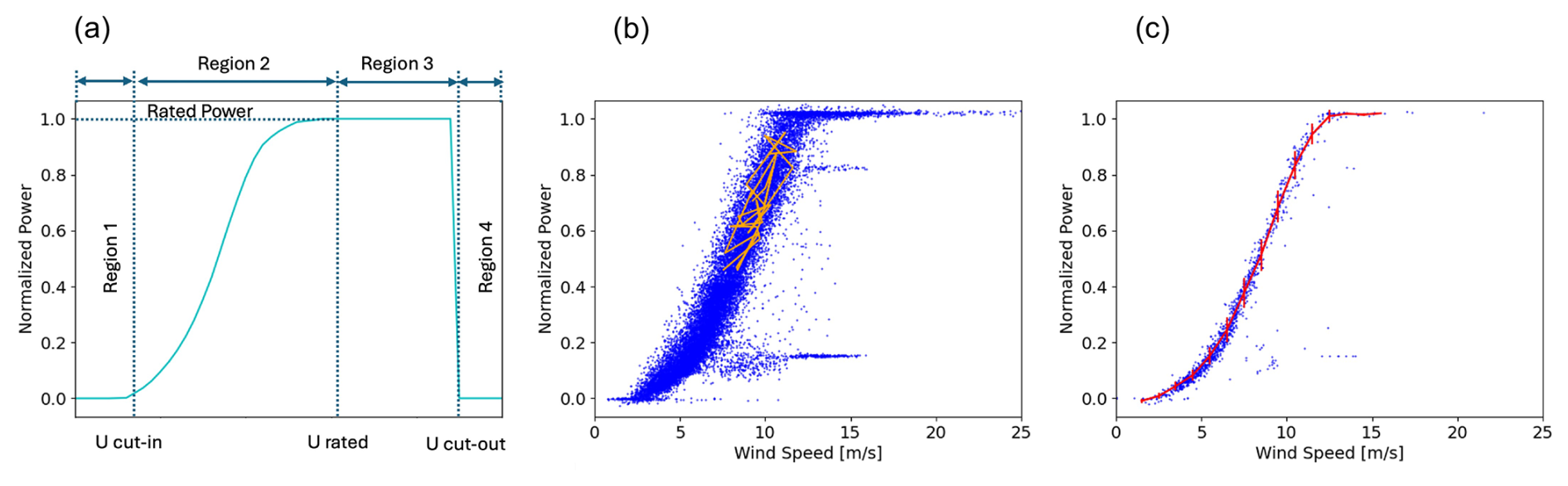
Figure 13 (a) Schematic of a wind turbine power curve showing operational regions; (b) power output of a wind turbine as a function of wind speed sampled at 0.5 Hz, with the orange line connecting a 5 min trajectory of the power wind dynamics (based on data used in Fig. 8 from Mahoney et al., 2012); and (c) IEC power curve from 10 min averaged data (blue dots), omitting outliers with error bars (red).

Figure 13b shows a scatter plot of the power output of a wind turbine as a function of wind speed measured upstream of the turbine rotor sampled at 1 Hz and then statistics calculated within a 10 min period. It is clear that there is a significant degree of scatter in the data. Many factors contribute to this scatter, which relates to both the unsteady, turbulent nature of the inflow wind profile and the ability of the turbine controller to respond to this rapidly changing wind profile. With stochastic methods, it is possible to partially disentangle these contributions (Lin et al., 2023).

To provide a meaningful estimate of the expected power output of a wind turbine as a function of wind speed, the IEC 61400-12-1:2022 standard (International Electrotechnical Commission, 2022) provides guidance on the measurement of a power curve. This is based on 10 min averages of concurrent wind speed and power measurements sampled typically at 1 Hz, which are then averaged in 0.5 m s⁻¹ bins. The standard also provides for corrections to be made for air density. A typical bin-averaged power curve is shown in Fig. 13c.

In its simplest form, the power curve is based on point measurements of 10 min averaged wind speed at hub height upstream of the rotor, ${\stackrel{\mathrm{‾}}{U}}_{\mathrm{H}}$. However, the shape of the wind profile will influence the power curve, and the use of a rotor-equivalent wind speed, ${\stackrel{\mathrm{‾}}{U}}_{\text{REWS}}$ (Sumner and Masson, 2006; Wagner et al., 2009), is recommended. In addition to wind shear, wind veer also impacts power production (Mata et al., 2024). Vratsinis et al. (2025) analyzed the performance of a large offshore wind farm and concluded that the IEC-defined rotor equivalent wind speed does not represent the full effects of shear and veer on a large offshore wind turbine. The level of turbulence intensity may affect the power curve. However, its effect on a power curve is not straightforward to determine as turbulence intensity is closely linked to other parameters that affect the wind profile, such as atmospheric stability, wind shear, and veer, which are interrelated. For example, stable atmospheric conditions will increase wind shear but will also increase veer and reduce turbulence intensity (and vice versa under convective conditions). Stability has been shown to affect the power curve (Antoniou et al., 2009; Wharton and Lundquist, 2012), but the direct impact of turbulent intensity cannot be easily quantified.

As a first consideration, 10 min averages do not truly reflect the total power in the wind (de Vries, 1978; Burton et al., 2001). Consider the instantaneous wind speed U:

$$\begin{array}{}\text{(17)}& {\displaystyle }{\displaystyle }U=\stackrel{\mathrm{‾}}{U}+U^{\prime },\end{array}$$

where $\stackrel{\mathrm{‾}}{U}$ is the 10 min averaged wind speed, and U^′ is an instantaneous fluctuation from the mean, assumed to be sampled from a normal distribution. Equation (16) tells us that the power in the wind is proportional to the cube of the wind speed (at least in Region 2) so that the mean power $\stackrel{\mathrm{‾}}{P}$

$$\begin{array}{ll}{\displaystyle }\stackrel{\mathrm{‾}}{P}\propto \left(\stackrel{\mathrm{‾}}{U^{\mathrm{3}}}\right)& {\displaystyle }=\stackrel{\mathrm{‾}}{(\stackrel{\mathrm{‾}}{U}+U^{\prime }{)}^{\mathrm{3}}}\\ {\displaystyle }& {\displaystyle }=\stackrel{\mathrm{‾}}{(\stackrel{\mathrm{‾}}{U}{)}^{\mathrm{3}}}+\mathrm{3}\stackrel{\mathrm{‾}}{{\stackrel{\mathrm{‾}}{U}}^{\mathrm{2}}{U}^{\prime }}+\mathrm{3}\stackrel{\mathrm{‾}}{\stackrel{\mathrm{‾}}{U}(U^{\prime }{)}^{\mathrm{2}}}+\stackrel{\mathrm{‾}}{(U^{\prime }{)}^{\mathrm{3}}}\\ {\displaystyle }& {\displaystyle }={\stackrel{\mathrm{‾}}{U}}^{\mathrm{3}}+\mathrm{3}\stackrel{\mathrm{‾}}{U}\stackrel{\mathrm{‾}}{(U^{\prime }{)}^{\mathrm{2}}}\\ {\displaystyle }& {\displaystyle }={\stackrel{\mathrm{‾}}{U}}^{\mathrm{3}}+\mathrm{3}\stackrel{\mathrm{‾}}{U}{\mathit{\sigma }}_u^{\mathrm{2}}\\ \text{(18)}& {\displaystyle }& {\displaystyle }={\stackrel{\mathrm{‾}}{U}}^{\mathrm{3}}(\mathrm{1}+\mathrm{3}{I}_u^{\mathrm{2}}),\end{array}$$

where I_u is the streamwise turbulence intensity. This means that, in theory, at least in Region 2, the 10 min wind speed will underestimate the turbine power, and this underestimate depends on the square of the turbulence intensity. This would hold for any convex curve relationship, where $\stackrel{\mathrm{‾}}{P}\propto U^n$ and n>1. Where n<1, it is straightforward to show from a Taylor expansion that an increase in I_u would be expected to reduce the expected power. This latter case is seen in Region 2.5, where the turbine controller deviates from optimum aerodynamic efficiency. There have been several studies that have supported this, showing that turbine power output is increased as I_u increases at low wind speeds above cut-in. Power output decreases with increasing I_u at higher wind speeds just below rated (Honrubia et al., 2012; Dörenkämper et al., 2014; Hedevang, 2014; Bardal et al., 2015; St. Martin et al., 2016; Lee et al., 2020; Kim et al., 2021; Sakagami et al., 2015, 2023); several methods have been proposed to correct power curves for this effect, e.g., Albers (2010), Clifton and Wagner (2014), Hedevang (2014), and Lee et al. (2020), and have generally been found to be effective.

The detailed effects of the scale, magnitude, and coherent structure of turbulence on the aerodynamic performance of a wind turbine have received less attention. In one of the few such studies, Gambuzza and Ganapathisubramani (2021) investigated the sensitivity of the power and thrust coefficients of a model horizontal-axis wind turbine (HAWT; 0.18 m rotor diameter) in a wind tunnel to conditions of various turbulence intensities and length scales. The C_P−λ curve was determined for different values of I_u, showing an increase in peak C_P as I_u was increased. However, this increase was significantly greater than expected from the dependence suggested in Eq. (18). This was attributed to the dependence of the blade aerodynamic properties on freestream turbulence and the resulting torque generated. The scale of the turbulence was also shown to impact performance, with longer turbulent timescales translating into higher power, which was not seen for higher-frequency turbulence. This was assumed to be due to the ability of the rotor to exploit the power of the lower-frequency fluctuations, which becomes increasingly difficult given inertia limitations as the fluctuations become faster. A similar wind tunnel study was carried out on a model vertical-axis wind turbine (VAWT; H-Darrieus type of width 0.5 m and height 0.8 m) (Molina et al., 2019). Here, too, an improvement in peak C_P was noted as I_u was increased, which could not be attributed to the additional power in the turbulent fluctuations expected from Eq. (18). Molina et al. (2019) suggested that this is a consequence of more favorable stall characteristics (stall delay) when the blades were at a high angle of attack. This condition occurs more frequently for vertical-axis wind turbines than for horizontal-axis wind turbines due to the different geometries. No dependence on turbulence length scale was noted, though length scale and turbulence intensity were not independently varied in this case, in contrast to Gambuzza and Ganapathisubramani (2021). A further study of a model VAWT very similar to that of Molina et al. (2019) concluded that turbulent length scale did have an impact on performance, with length scales less than or similar in size to the blade chord length showing enhanced performance compared to a length scale much greater than the chord, which showed significantly lower performance (Peng et al., 2019). Clean flow gave rise to even lower performance. The authors speculate that the small-scale turbulence contributes to boundary layer re-energization around the blades, delaying flow separation and stall. Other work (Chamorro et al., 2015; Tobin et al., 2015) suggests that such findings may also hold for large-scale utility turbines. However, further work would seem justified, particularly with respect to the sensitivity of blade aerodynamics to turbulence when close to stall. There are potentially important differences in how HAWTs and VAWTs respond to turbulence, which requires further investigation, particularly if vertical-axis technology is used offshore or in the urban environment. While these wind tunnel studies were characterized by Reynolds numbers several orders of magnitude lower than those characteristic of conditions under which utility-scale turbines operate, Miller et al. (2018, 2019) used a high-pressure wind tunnel to achieve dynamic similarity to study both vertical- and horizontal-axis wind turbine power performance. Conducting experiments at a range of rotor-diameter-based Reynolds numbers, they have shown that the scale effects can significantly impact horizontal-axis turbine performance. However, they observed Reynolds number invariance of the power coefficient as a function of tip speed ratio for a cord-length-based Reynolds number greater than 3.5×10⁶ for a horizontal-axis wind turbine and 1.5×10⁶ for a vertical-axis wind turbine.

While controlled wind tunnel experiments can provide a wealth of data, the findings from these studies must be complemented with field studies. However, the complexity of field studies and limitations of wind tunnel experiments represent a challenge to bridging the gap between the two approaches and establishing a comprehensive understanding of how flow turbulence characteristics impact wind turbines. Designing a study that would include both wind tunnel experiments and field observations could be a step toward developing more complete insights into turbulence effects on power production.

7.2 High-frequency power oscillations

The effect of turbulence on the temporal behavior of turbine power output is important from the point of view of power quality. A study combining detailed field measurements with LESs (Nandi et al., 2017) concluded that turbine power output was sensitive to the passage of energy-containing atmospheric eddies, causing fluctuations on the scale of ∼10–100 s, but was relatively insensitive to the higher-frequency fluctuations of ∼1 Hz or greater associated with the sampling of small-scale turbulence by the blades.

One central drawback of the common method used to estimate the power output is that all fluctuations caused by the response of the wind turbine to the fast wind fluctuations are averaged out by the common 10 min mean values. Another approach is to use the fluctuations as response information in the wind energy conversion process. Using highly fluctuating data at 1 Hz or higher, it could be shown that power characteristics can be defined using stochastic process modeling, representing the evolution of a random value based on the Langevin equation (Eq. 19).

$$\begin{array}{}\text{(19)}& {\displaystyle }{\displaystyle \frac{\mathrm{d}P\left(t\right)}{\mathrm{d}t}}=D_{\mathrm{1}}(P,u)+\sqrt{D_{\mathrm{2}}(P,u)}\mathrm{\Gamma }\left(t\right)\end{array}$$

Here, P(t) denotes the power output, D₁(P,u) is the drift coefficient, D₂(P,u) is the diffusion coefficient, and Γ(t) denotes the zero-mean Gaussian noise. The coefficients are functions of the power output P and the wind speed u. The Langevin approach is independent of the site-specific turbulent wind features (Mücke et al., 2015). This methodology can also be extended to load estimations (Lind et al., 2014).

Analysis of smaller scales or higher frequencies of the power output of wind turbines shows that the wind energy conversion process is influenced by small-scale turbulence. The power output of even large wind turbines shows fluctuations of the order of a second (Milan et al., 2013, e.g., Table II). The statistical analysis shows that turbulence, including remarkable features of intermittency (i.e., non-Gaussian statistics), drives power fluctuations. Stochastic models for non-Gaussian frequency fluctuations are presented in Schäfer et al. (2018). Milan et al. (2013) showed that these fluctuations are not averaged out and can significantly impact the power output of entire wind farms. Haehne et al. (2018) analyzed fast frequency fluctuations of the power grid and showed that these are related to wind power fluctuations. Therefore, even country-wide-averaged wind power carries the imprint of turbulence.

Power quality is a major challenge for the grid integration of renewable generators (Liang, 2017). The turbulent nature of wind energy has led to investigations of the impact of intermittent power feed-in on power grids (Schmietendorf et al., 2017; Auer et al., 2017). Numerical results indicate that intermittency propagates in a power grid and affects the frequency increment distributions of nodes distant to the feed-in. The principle problem and a gap in our ability to develop an effective approach to mitigate the effect of turbulence in high-frequency power fluctuations is that the intermittent, non-Gaussian statistic does not fall into any well-defined mathematical category. Only phenomenological formulas are known. This results in significant uncertainties when estimating the probability of extreme events of power fluctuations.

7.3 Impacts of certain atmospheric phenomena

7.3.1 Low-level jets

Over the past 2 decades, several billion dollars have been invested in installing large wind farms in the Great Plains region of the US, including in Texas, North Dakota, Oklahoma, and Kansas. Nocturnal LLJs frequently occur in this region, and it is common knowledge in the wind energy community that LLJs make wind resources more favorable for power production (e.g., Kelley et al., 2006; Storm and Basu, 2010; Wimhurst and Greene, 2019). The Wind Forecast Improvement Project report (Wilczak et al., 2015) stated the following:

Qualitative analysis indicates that the LLJ is a regular, periodic, … and dominant feature in the SSA [Southern Study Area in Texas] that drives capacity factors to over 60 % (and therefore a large fraction of power production) during the nocturnal hours.

A few modeling studies have attempted to quantify the importance of LLJs more systematically. Cosack et al. (2007) used observed wind profiles from a SODAR deployed in Germany as input for the FLEX5 aeroelastic simulation tool. Using 1.5 and 5 MW wind turbine models, they found that LLJs increase power production, and the effect increases as turbines become higher. Similar conclusions were reported by Gutierrez et al. (2016) and Weide Luiz and Fiedler (2022). Gutierrez et al. (2016) used high-frequency measurements from a 200 m tall met mast near Lubbock, Texas, as input for the FAST (Jonkman and Sprague, 2024, now OpenFAST) model to model power production. Weide Luiz and Fiedler (2022) used power curves from utility-scale turbines (Enercon E-126 and Vestas V112), in conjunction with lidar observations from two locations in Germany.

Wind turbines cause enhanced turbulent mixing and, therefore, affect LLJ profiles in the presence of wind farms. In recent work, Gadde and Stevens (2021b) employed LES, with actuator disks representing turbines, to simulate wind power production during LLJ conditions. They found that when the nose of the LLJ is above the turbine, the lost production of downstream turbines is relatively low, as energy can be entrained from the jet above the wind farm. Also, Doosttalab et al. (2020) found that wind farm energy production can benefit from enhanced air entrainment from the jet. As a result of the momentum extracted by the turbines, the jet's strength is reduced, and the wind shear at lower altitudes is affected (e.g., Abkar et al., 2016; Larsén and Fischereit, 2021; Quint et al., 2025). Large wind farms can deflect part of the jet over the wind farm, as large wind farms, in general, deflect flow; see, e.g., the mesoscale modeling study of Larsén and Fischereit (2021) and idealized LES cases. When the jet nose lies below the turbine hub, turbulent kinetic energy from the jet is transported upwards instead of downwards such that downstream turbines can benefit from the LLJ's energy (Gadde and Stevens, 2021a).

Although LLJs and their impacts on wind energy have been studied extensively in specific regions (e.g., Emeis, 2014; Aird et al., 2022), there is still a lack of observed wind speed and direction profiles associated with LLJs, particularly for offshore and coastal conditions (Shaw et al., 2022). Towers typically only reach 100–200 m, and sodars are frequently rendered ineffective in the layer near the LLJ nose due to the lack of shear-produced turbulence. While profiling (floating) lidars can provide more information (Wagner et al., 2019), they are expensive, not routinely used, and typically have a vertical range of approximately 200 m. These measurements should also provide more information about the turbulence structures near and above the LLJ nose.

7.3.2 Mesoscale convective circulations – rolls and cells

The fluctuations in wind speed associated with the presence of convective cells represent great challenges for power-balancing systems (Akhmatov et al., 2007; Sørensen et al., 2008). Sørensen et al. (2006) compared the wind power from the offshore farm Horns Rev and onshore turbines on 18 January 2005, showing that the offshore power fluctuates sharply, while it is stable onshore. Open cells were present that day over the North Sea following a frontal passage.

Vincent (2010) systematically studied the intra-hourly fluctuating wind characteristics in connection with open cells and their impact on offshore wind power for the North Sea region. Larsén et al. (2013) showed that a collection of 18 cell cases have spectral energy that is 5 times larger than the climatological mean value in the range of about 10⁻⁴–10⁻³ Hz. Imberger et al. (2013) showed that the distribution of the wind speed change, δ_U, between two consecutive 10 min values in the presence of open cells suggests significant changes and deviation from that in the absence of cells. Vincent and Trombe (2017) reviewed the topic of forecasting the intra-hourly variability in wind generation. Göçmen et al. (2020) compared the wind power variation in the Horns Rev farm in the presence and absence of open cells using 10 min mean and 1 min SCADA data. While the mean wind conditions are comparable for the two cases, the turbulence intensity, variation in wind direction, and power fluctuation are systematically and significantly larger in the presence of open cells than in the absence of them.

Organized structures such as cells not only bring large fluctuations at one single point, but also provide spatial variations and coherence (Vincent et al., 2013; Larsén et al., 2013, 2019), which will also challenge some of our methods where standard coherence models are used, e.g., in connection with power balancing.

Cells contribute to the intra-hourly variability in wind, power, and the microscale regime. Larsén et al. (2019) analyzed the turbulence characteristics of wind during a cell event using sonic measurements from two stations. They showed that the open-cell-related variability tends to fill the spectral gap with extraordinary energy, affecting the power spectrum from about 0.0002 to 0.01 Hz. Accordingly, using typical boundary layer models, even considering scaling with boundary layer height, significantly underestimates the turbulence intensity. The sizes of open cells have important implications and challenges for the methodologies used in wind energy. Currently, when calculating turbulence-related parameters such as load, turbulence intensity, gust, and wake meandering, only scales smaller than the spectral gap are considered using typical boundary layer models such as Kaimal et al. (1972), Veers (1984), and Mann (1998). The spectral gap is typically assumed to be at a wavelength of 1 km or a period of 10 min–1 h. The concept of the gap has been used to filter out larger-scale variability (Larsén et al., 2016). The flow through large wind farm clusters therefore involves both micro- and mesoscales. With a typical roll width of 2–10 km and cell diameters from a few kilometers to 40 km, it is expected that they can both affect the performance of turbines and wind farm clusters.

While several studies have addressed the effects of convective cells on wind energy production in wind farms in the North Sea, the effect of mesoscale convective rolls has not yet been studied. Cold-air outbreaks along the US East Coast result in convective rolls, which are evident in satellite images as cloud streets. Atmospheric conditions under which convective rolls occur are characterized by a lower magnitude of the stability parameter, the ratio of mixed-layer height, z_i, and Obukhov length, L, in comparison to convective cells ($|z_i/L|<\mathrm{20}$) as a result of stronger winds and a shallower mixed layer. Future studies should focus on the impact of these flows on power production.

7.3.3 Gravity waves

A modeling study of a hypothetical large offshore wind farm suggested that when an AGW of the same size as the wind farm was present, a swing in power production from the highest-producing turbine to the lowest of 76 % was possible compared to a control situation with a similar upstream wind speed with wake effects only where a swing of just 29 % was observed (Ollier et al., 2018). Studies of the impact of AGWs on operating wind farms are scarce, which is surprising considering their prevalence (Nappo, 2013). One of the few such studies looked at a wind farm downstream of the Cascade Range mountain chain in the US (Draxl et al., 2021). In this study, measurements from turbines within the wind farm were compared with mesoscale model simulations. Figure 14 shows the results for one such wind turbine. As the turbine was operating close to rated power, significant fluctuations in both wind speed and power production were observed. Due to the presence of AGWs, the aggregated wind farm output fluctuated by 11 %.

Figure 14 (a) Comparison between observations and mesoscale model (WRF) simulations for a wind turbine within a wind farm experiencing AGWs (adapted from Draxl et al., 2021, licensed under CC BY 4.0 license). (b) LES of a flow in the Columbia River Gorge area, during the WFIP2 field study, resolving atmospheric gravity waves (courtesy of Scott Pearse and Pedro Jiménez).

In addition to experiencing the effect of “naturally occurring” AGWs, Smith (2010) proposed that the wind farms themselves could induce gravity waves, which can affect their performance. Smith (2010) developed a linear quasi-analytical model of the effect of a large operating wind farm on atmospheric flow due to turbine drag, resulting in the exchange of momentum with the free atmosphere and generation of gravity waves under stable atmospheric stratification. The combined resistance presented by an array of turbines due to their thrust acts similarly to an orographic feature. More recent research has used LES models to investigate the coupling between AGWs and semi-infinite wind farms, wind farms finite in the downstream direction but infinite in the crosswise direction (Wu and Porté-Agel, 2017; Allaerts and Meyers, 2017, 2018). It has been shown (Allaerts and Meyers, 2017) that a large wind farm can form an internal boundary layer that displaces the ABL aloft, exciting AGWs.

Numerical simulations predict significant pressure fluctuations that adversely impact wind farm efficiency. Wu and Porté-Agel (2017) suggested that the first row of turbines in a wind farm can experience greater than a 35 % reduction in power output in the presence of a strong inversion. However, turbines at the rear of the wind farm may see an increase due to an advantageous pressure gradient accelerating the wind speed. Allaerts and Meyers (2019) developed an extended and improved version of a model developed by Smith (2010) using three layers to investigate the coupling between wind farm layout and AGWs. The work suggested that gravity wave effects are small for very wide or long wind farms. Lanzilao and Meyers (2021) used the three-layer model developed in Allaerts and Meyers (2019) to explore how advanced wind farm control could mitigate the impact of wind-farm-induced AGWs on performance, showing that gains of up to 14 % could be achieved in certain cases. While numerical studies point to the potentially significant impact of wind-farm-induced AGWs on wind farm performance, the significance and impact of these effects on power production have not been confirmed yet by observations. One of the goals of the recent field study, the American Wake Experiment (AWAKEN), is to study and characterize the effect of AGWs on wind power production (Moriarty et al., 2024).

Modeling of wind-farm-induced AGWs is still a challenge. Avoiding nonphysical wave reflections and their amplification requires very large domains and damping layers. The most optimal way to do this has not been determined, leading to time-consuming simulations with no guarantee that numerical artifacts will not affect the validity of the results. A limited range of atmospheric conditions and wind farm layouts has been investigated. A much wider range of investigations is required to gain better insights into the coupling between AGWs and wind farm performance, combining detailed measurements from satellites and lidars with high-resolution mesoscale and microscale modeling. A better understanding of the impact of both naturally occurring and wind-farm-induced AGWs on loading and performance is required. However, since spatial fluctuations in wind speed across a wind farm are frequently significant, one of the key challenges is distinguishing the impact of AGWs from other atmospheric phenomena. Access to wind farm data will also be key for model validation and investigating the extent to which AGWs impact wind farm generation and loads onshore and offshore.

7.4 Topographic effects

A large fraction of wind energy capacity has been deployed in regions with excellent wind resources in relatively flat, homogeneous terrain or offshore. The projected growth of wind power deployment worldwide will, by necessity, lead to more wind farms being developed in complex terrain. In general, we can define complex terrain as terrain characterized by heterogeneity of topography or land use, possibly including forested terrain. Most of the studies of flows in complex terrain for wind energy applications have focused on complex topography, and therefore, in what follows, we will focus on topographic effects on wind power production and wind turbine loads.

Some of the first studies of flows in complex terrain related to wind energy applications were conducted in the early to mid-1990s (Taylor and Smith, 1991; Stefanos et al., 1994, 1996) and focused on measurement and steady numerical simulations of topographic wakes. These studies were limited in scope and complexity due to limitations in observing systems and computational resources. Over the last 30 years, the development of remote sensing technology (e.g., Doppler lidars) and high-performance computing now enables more detailed studies of flows in complex terrain. In contrast to RANS, which was used in early studies (e.g., El Kasim and Masson, 2010), nowadays, LES can better account for terrain-induced circulations combined with the effects of atmospheric stability, often resulting in highly unsteady flow. Yang et al. (2021b) reported on one of the first LESs of a flow through a utility-scale wind farm in complex terrain, the Invenergy Vantage wind farm in Washington State, US. They used the Virtual Flow Simulator (VFS-Wind) code and computed mean power and the root mean square (RMS) of power fluctuations. The agreement between simulations and observations indicated that LES could be used to optimize wind farms sitting in complex terrain. Similarly, Tabas et al. (2021) found good agreement between simulated and measured wind farm power when using the RANS model WindSim. However, they also found that the results were sensitive to model parameters. Because LES models resolve large turbulent eddies, it is likely that LES results would be less sensitive to the choice of turbulence model parameters than RANS.

Although there is a relatively small number of LESs of flows through wind farms in complex terrain, these simulations span a range of configurations, from idealized LESs of flow over two-dimensional hills and valleys between them (Liu and Stevens, 2020, 2021) to simulations of observed flows through wind farms in complex terrain. Complex topography can result in a wide range of flow configurations, particularly when combined with atmospheric stability effects. In addition to the mountain-induced AGWs discussed earlier, some of the flow phenomena that can have a significant impact on the level of turbulence and, therefore, on turbine loads and wind power production are wind speed-up on ridges, topographic wakes, up- and down-valley flows, cold pools, and gap flows. These flow phenomena can result in elevated turbulence or intermittent turbulence levels that can significantly impact turbine performance through power production and increased turbine loads. Turbulence can also play an indirect role in power production by mixing out cold pools characterized by low wind speeds, thus inducing wind ramps. The diversity of phenomena represents a challenge for developing a general approach to characterizing turbulence in complex terrain and its impacts on wind turbine and wind farm performance.

As previously indicated, several field studies have focused on better characterization of topographic effects for wind energy applications in recent years. For example, the WFIP2 field study occurred in the Columbia River Gorge area east of the Cascade Range, where more than 5 GW of wind power is already deployed. This is affected by the mountain wake from Mt. Hood, a cone-shaped, volcanic mountain rising 3000 m above the surrounding landscape. Under favorable atmospheric stability conditions, von Kármán vortices are frequently shed from islands and isolated mountains like Mt. Hood. Mountain-wake-induced wind speed reduction or even wind reversal associated with von Kármán vortices directly impacts wind power production in the lee of mountains and islands. Under stably stratified atmospheric conditions, topographic effects include the formation of cold pools in valleys. Cold pools are decoupled from the flow aloft and can persist for extended periods (McCaffrey et al., 2019). Because cold pools are associated with reduced wind speeds and reduced wind power production, accurate forecasting of cold-pool formation, maintenance, and eventual mix-out is essential for effective wind resource assessment and wind power utilization (e.g., Olson et al., 2019; Bianco et al., 2019). Arthur et al. (2022) demonstrate that more accurate prediction of cold-pool mix-outs could be achieved by a mesoscale model accounting for horizontal turbulent mixing using a three-dimensional planetary boundary layer parameterization (3D PBL; Kosović et al., 2020; Juliano et al., 2022).

It may be considered beneficial to site wind turbines near escarpments or on the top of steep ridges. However, the effects of topographically induced flows and associated turbulence can negatively impact horizontal-axis turbine performance (Lange et al., 2017). Dar and Porté-Agel (2024) designed a wind tunnel experiment to study the effect of different wind directions on the flow over an escarpment. They found that the recirculation zone over the escarpment disappears if the angle between the wind direction and normal to the escarpment is greater than 15°. According to their study, this wind direction results in the largest normalized TKE level.

Clifton et al. (2022) recently reviewed research challenges for wind energy in complex locations, including complex terrain, and concluded that a focused research and development effort is required to ensure that deployment of wind energy at complex sites is competitive. To enable more rapid progress, they recommend developing new frameworks for sharing data and test facilities in complex terrains and diverse climate zones spanning a wide range of weather patterns. Furthermore, they point out that there is no widely accepted definition of “complex terrain” for wind energy applications. The recent IEC 61400-1 standard (International Electrotechnical Commission, 2019a) categorizes complex terrain as low, medium, and high complexity as a function of slope angles and terrain variance. As challenges, Clifton et al. (2022) point out the lack of standards for power performance testing at complex sites because the freestream wind speed cannot be identified easily. In addition, wind resource assessment and wind power forecasting are challenging due to the numerical resolution requirements.

8 Impact of turbulence on loads

An understanding of the expected range of turbulent inflow conditions is essential in the design of wind turbines. Turbulence is the principal driver of fatigue, and its spatial and temporal structure has a significant impact on the lifetime of a machine. Responses of different materials to turbulence vary significantly, and there needs to be a robust way to calculate the expected lifetime of the different wind turbine components operating in any situation. Calculations of parameters such as damage equivalent load (DEL) are generally based on relatively simple parameterizations of the wind inflow with constant wind shear and veer and a constant mean flow, possibly with a simple stochastic turbulence model or a deterministic gust profile superimposed. However, the turbulent properties of real inflow can deviate significantly from these simple assumptions. Phenomena such as low-level jets, intermittent events, downbursts, or typhoons can create transient turbulent inflow fields that differ markedly from the mean and cannot be captured using simple turbulence models or gust profiles.

In the context of atmospheric turbulence and determining its impact on loads, the IEC standards (IEC 61400-1, International Electrotechnical Commission, 2019a, and IEC 61400-3-1, International Electrotechnical Commission, 2019b, for offshore wind energy) play a significant role. The purpose of these standards is to provide a standardized set of definitions, rules, requirements, and guidelines for wind energy applications. In principle, the standards have two major objectives:

1. to classify turbines according to a given set of design load cases dependent on external conditions and

2. to characterize the local external site conditions, i.e., to verify that the local conditions are not more severe than the turbine class selected.

Design load cases are specified for a large range of wind turbine operational conditions, e.g., power production, fault, start-up, and parked, under different environmental conditions determined to be either normal or extreme. The latter is furthermore specified for different gust situations and extreme turbulence. Specific guidelines are given for the generation of synthetic turbulent inflow.

The standardized wind conditions and models in the IEC standards are subject to several simplifications, which, given today's huge turbines with rotor diameters of more than 200 m and hub heights of the same order of magnitude, seem too simplistic. The most important simplification is the prescription of a constant shear exponent across the full rotor, as described in Eq. (10), with zero veer across the rotor. Turbulence is assumed to be homogeneous, conforming to either the Kaimal (Kaimal et al., 1972) or the Mann model (Mann, 1994).

Actual conditions at turbine sites need to be better understood and characterized since, in some situations, fatigue damage could exceed values calculated using the assumptions of the prescribed models in the standards. The following sections look in more detail at the shortcomings of the IEC standards and describe several of the phenomena not (fully) accounted for in the standards whose turbulent properties require further research.

8.1 Limitations of the design standards

This section begins by assessing the validity of the assumptions made in the IEC standards in the context of a well-established literature on boundary layer meteorology, atmospheric turbulence, and wind engineering (Panofsky and Dutton, 1983; Oke, 1987; Stull, 1988; Simiu and Scanlan, 1996; Arya, 1999, 2001; Holmes, 2007). The IEC 61400-1 standard for wind turbine design recommends two turbulence models to account for atmospheric turbulence: the Mann spectral tensor model (Mann, 1994) and the Kaimal spectral model (Kaimal et al., 1972) with the exponential coherence model by Davenport (1961). The corresponding Kaimal and Mann spectral formulations are stationary models designed for neutral atmospheric conditions in the surface layer. These models and the employed parameters, which are based on measurements from relatively short meteorological masts (e.g., Kaimal et al., 1972), have limitations in presenting inflow conditions accurately, especially for modern turbines that nowadays operate outside the surface layer.

Based on measurements collected from a flat, uniform field site in Kansas, Kaimal et al. (1972) proposed several generalized spectra (and co-spectra) functions for various variables. The velocity spectra exhibit a pronounced and systematic dependence on measurement height, wind speed, and atmospheric stability (see also Panofsky and Dutton, 1983). The study derived simplified velocity spectra functions for neutral conditions from the more general ones to facilitate comparisons with wind tunnel and other observational data. These simplified functions were solely dependent on height and wind speed. In subsequent work, International Electrotechnical Commission (2005) further modified and simplified these longitudinal velocity spectra for design purposes. However, it is well-documented that the characteristic sizes of turbulent eddies decrease as atmospheric stratification increases (e.g., Stull, 1988). Consequently, coherence typically diminishes more rapidly under stably and neutrally stratified conditions than under unstable conditions (Panofsky and Dutton, 1983). However, the IEC exponential coherence model (International Electrotechnical Commission, 2019a) does not incorporate such stability-dependent variations. Furthermore, for the sake of simplicity, the IEC guidelines assume that the integral length scale remains unchanged with height for hub height z_h>60 m within the turbine rotor layer, resulting in spectra that no longer account for height dependence. While simplifying height dependence was a reasonable approximation for smaller rotors (around 20 m), this assumption is not physically realistic for modern rotors, in particular when operating in a relatively shallow stably stratified ABL.

According to IEC standards, standard industry tools such as TurbSim (Kelley and Jonkman, 2007) and the Mann turbulence generator (e.g., Dimitrov et al., 2024) provide stationary Gaussian wind fields with uniform variance and predefined spectrum and coherence properties. However, wind turbines in the field are subject to atmospheric turbulence, which can significantly affect their power output, loading, and fatigue life. For high-Reynolds-number turbulent flows, as observed in the atmosphere, the pdf's of velocity increments portray strong non-Gaussian behaviors (e.g., heavy tails) for small spatial–temporal separations (Frisch, 1995; Bohr et al., 1998; Basu et al., 2007; Mücke et al., 2011). For large values of separations (of the order of the integral scale), these pdf's asymptotically approach the Gaussian distribution. The scale dependence of the velocity increment pdf's, a characteristic feature of the multifractal cascade dynamics of turbulence, should be accurately reflected in inflow as this turbulence structure is crucial for understanding the structural loads and performance of the turbine under realistic conditions. A preliminary LES study suggests that a large, utility-scale turbine acts as a low-pass filter, and therefore the non-Gaussian effect alone does not significantly impact fatigue loads of the turbine (Berg et al., 2016).

Considering the above facts, it becomes apparent that contemporary turbine inflow generation approaches have many limitations and that a paradigm change is needed. Working towards this goal, researchers from the National Renewable Energy Laboratory (NREL) (Jonkman, 2009) implemented a capability in TurbSim to include coherent structures that reflect the proper spatiotemporal turbulent velocity field relationships seen in instabilities associated with nocturnal boundary layer flows (e.g., breaking Kelvin–Helmholtz waves) and which are not represented well by the IEC Normal Turbulence Models. TurbSim provides the ability to efficiently generate randomized coherent turbulent structures produced by one of the non-neutral spectral models that are superimposed on the more random background turbulent field characterized by non-zero coherence.

LES is an attractive way to generate inflow winds with non-Gaussian statistics as it simulates unsteady, anisotropic turbulent flows dominated by large-scale structures and turbulent mixing that are all characteristic of the atmosphere (Berg et al., 2020). Many atmospheric phenomena, including thermal stratification, can be well represented in LES. A comparison with field data shows that high-frequency content is typically not fully represented in LES and requires even higher-fidelity modeling (e.g., Mirocha et al., 2018). Additionally, in idealized canonical LES cases, lower frequencies are underestimated compared to field measurements, as the impact of mesoscale atmospheric dynamics (e.g., mesoscale convective circulations) is not accounted for (e.g., Sim et al., 2023). Meanwhile, it has been shown that accounting for the lower frequencies is important, especially offshore and for bigger rotors (Syed and Mann, 2024). Comparisons between IEC model spectra and LES and field measurement data reveal that IEC models capture neutral stratification better than stable and unstable conditions.

Point statistics, such as wind speed and turbulence intensity at hub height, significantly impact a wind turbine's response. However, for larger rotors where the spatial and temporal distribution of the wind field becomes increasingly important, factors like wind shear and related turbulence anisotropy, inhomogeneity, and coherence (Eq. 14) become more important.

The common approach in the wind energy industry neglects quad coherence as it is generally assumed to be less significant than co-coherence. While quad-coherence is generally smaller than co-coherence, it is certainly not negligible. This assumption may be significant in terms of the loads experienced by a wind turbine blade, as turbulent velocity fluctuations at a certain frequency may not exhibit the same phase along the length of the blade. The coherence model associated with the Kaimal spectrum model in the IEC standard does not account for quad-coherence. The Mann model includes quad-coherence; however, it is not explicitly included in the IEC standard. TurbSim uses the Davenport coherence model (Davenport, 1961), which neglects quad-coherence; however, HiperSim (Dimitrov et al., 2024) provides turbulence generation capability based on the Mann model. The algorithm windSim4D, developed by Cheynet et al. (2022), includes quad-coherence and relaxes Taylor's frozen turbulence requirement. Cheynet et al. (2022) indicated that quad-coherence does not affect linearized wind load estimates.

In recent years, the Mann model has been extended to account for a wider range of atmospheric phenomena that impact wind turbine performance. Segalini and Arnqvist (2015) extended the Mann model to account for stable stratification, while Chougule et al. (2017) further extended the Mann model to account for the full range of atmospheric stability and introduced two new parameters, gradient Richardson number, Ri, and temperature variance destruction, η_θ. They compared statistics of uniformly stratified and sheared model-generated turbulence to observations from the HATS field study (Horst et al., 2004). Since these models did not account for low-frequency fluctuations induced by two-dimensional, mesoscale motions, Syed and Mann (2024) extended the Mann model to include length scale corresponding to the peak of mesoscale turbulence, the boundary layer height, and the variance due to two-dimensional, low-frequency fluctuations in addition to the anisotropy parameter. Further developments are needed to include conditions when the mesoscale peak is not pronounced, such as in the presence of mesoscale convective circulations. The Mann model was also extended to the space–time domain (de Maré and Mann, 2016; Guo et al., 2022). These are important developments toward a better characterization of turbulence in an ABL that warrant further studies to evaluate how these models perform under a range of conditions.

Although new developments have led to a more complete and realistic representation of atmospheric conditions, several phenomena are still absent in current inflow models that are likely to impact design loads significantly. For instance, design inflow conditions do not account for veer. Despite the numerous identified inaccuracies and instances of incomplete or missing data in current inflow models, the industry has not experienced frequent failures of primary structures. This suggests that assumptions of overly energetic inflow turbulence and generous safety factors have led to conservative designs. However, the scale of modern-day wind turbines is such that inaccuracies in existing inflow models may be inadequate for cutting-edge design and optimizing safety margins.

Flow conditions, characterized by anisotropic, intermittent turbulence, result in dynamic instability, leading to flow-induced vibrations and blade flutter, which cause unsteady aerodynamic forces. Dimitrov et al. (2017) quantified the impact of turbulence length scales and anisotropy associated with normal and extreme turbulence on fatigue and extreme loads. They concluded that compared to the observed standard deviation of turbulence in the IEC 61400-1 Ed. 3, the standard deviation is underestimated. Perturbations due to turbulence can result in large vortex-induced vibrations (Grinderslev et al., 2022). As the size of wind turbines increases, so does the impact of vortex-induced vibrations (Grinderslev et al., 2023). Naqash and Alam (2025) provide a review of the impact of flow-induced vibrations on turbine blade loads, fatigue, and failures.

Furthermore, we note that extreme atmospheric turbulence events, such as hurricanes, thunderstorms, and downbursts, exhibit spatial and temporal characteristics that differ significantly from IEC design load cases, necessitating separate considerations. For further insights into how inflow conditions influence wind turbine design, we refer to Veers et al. (2023).

Achieving better estimates of the boundary layer turbulence impact on fatigue loads and wind power production requires better characterization and representation of turbulence as modulated by complex atmospheric conditions at elevations of modern wind turbines (i.e., outside the surface layer). This should also include offshore environments. Improving the representation of dynamically evolving turbulent flows in high-resolution simulations (i.e., LES) necessitates including low-frequency, mesoscale-induced fluctuations. This can be achieved by going beyond idealized setups and embracing fully coupled mesoscale to microscale simulations, as discussed in Sect. 3.6.

8.2 Impact of atmospheric phenomena on fatigue loads

The fatigue loading experienced by turbines is a crucial design consideration outlined in the IEC 61400 standard for wind turbine safety (International Electrotechnical Commission, 2019a). The IEC provides certified standards for various well-defined turbine types. Before construction, it needs to be verified that the site-specific conditions are within the limits of the turbine type certification. Wind conditions at a site are specified by extreme wind speed, vertical wind shear, flow inclination, turbulence, and rare gust-like events. The load type is either an ultimate load that damages the turbine or a fatigue load. While turbine classification is the responsibility of turbine manufacturers, site assessment is in the hands of project developers and requires insight into atmospheric turbulence dynamics. However, the IEC 61400 standard does not define turbulence intensity consistently. First it defines it based on wind speed and later based on longitudinal velocity.

Wind conditions are determined using simplified models, scaled by hub height values, providing a reference wind speed and turbulence intensity. The effective turbulence intensity is an ideal turbulence intensity, independent of wind direction, to characterize a site such that fatigue damage is expected to be representative of the wind conditions encountered at the site. However, atmospheric turbulence and wind speeds typically depend on wind direction and atmospheric stability. They are often correlated due to upstream conditions at the site or in relation to certain weather phenomena. On the other hand, turbine damage is highly non-linearly related to loading amplitudes and, therefore, to turbulence intensity. As a result, a few extreme events may cause the most fatigue damage, and the concept of an effective turbulence intensity fundamentally cannot capture the richness of atmospheric turbulence. By definition, turbulence intensity is inversely proportional to wind speed, and therefore under certain extreme wind conditions, such as downslope wind storms (Pehar et al., 2019), it is not a good predictor of fatigue loads. Furthermore, turbulence generated by upstream turbines impacts downstream turbines. The work by Frandsen (2005) has led to the incorporation of wake-added turbulence of neighboring turbines to the effective turbulence intensity, and a simple wake turbulence model is provided for this.

Wind turbine wakes affect the dynamic loading on the turbines due to increased turbulence, the created wind speed deficit, and changes in turbulence structure. Thomsen and Sørensen (1999) used the Vindeby experiment combined with the aeroelastic code HAWC to demonstrate that turbulence intensity, length scales, and coherence are parameters that strongly affect turbine loading. They found that loads for a turbine installed in an array or a farm are approximately 5 % and 15 % higher than those in freestream conditions, and the increase is similar onshore and offshore. Turbine loads are typically higher onshore than offshore as turbulence intensity is typically lower offshore (Dahlberg et al., 1992). This is also supported by LES studies conducted by NREL (Churchfield et al., 2012; Lee et al., 2013), which capture the structural load experienced by wind turbines by using the FAST model coupled to the LES. They found that increased surface roughness, typical for onshore conditions, increases damage equivalent loads on the turbines. Furthermore, they showed that downstream turbines typically experience more significant damage than loads. However, the in-plane blade root moments for downstream turbines are lower due to the lower wind speed.

Thomsen and Sørensen (1999) showed that fatigue loads are higher when the turbulence spectral length scale is smaller. Riziotis and Voutsinas (2000) showed that yaw misalignment can increase fatigue loads. Furthermore, they state that the higher turbulence intensity is the main cause of higher turbine fatigue loads in complex terrain. The Vindeby (Frandsen and Thomsen, 1997) and Sexbierum (Adams, 1996) experiments showed that fatigue loads are similar in single- and multiple-wake situations, which supports the view that the wake-added turbulence intensity of the closest turbine is the most relevant. Here, we point out that the turbulence magnitude defined by Eq. (3) may stay constant through the row of wind turbines, while the intensity of turbulence, a non-dimensional value, would increase because the wind speed in the wake may decrease. However, it should be noted that LES has shown that, depending on the wind farm layout, turbulence levels in the wind farm can increase in the downstream direction for multiple turbine rows. Studying yaw control for a wind turbine and a wind farm, Damiani et al. (2018) concluded that turbulence intensity is one of the primary causes of damage equivalent loads.

Sathe et al. (2013) and Holtslag et al. (2016) showed that the lifetime fatigue loads experienced by a wind turbine depend strongly on the joint probability distribution of hub height wind speed and atmospheric stability. Typically, IEC standards are followed, and atmospheric stability is neglected. Lee et al. (2018) showed that the relative positioning of turbines matters when loading is concerned. Displaced downstream turbines that experience partial wake impingement are subjected to significantly larger fatigue loads compared to a fully waked turbine. Lee et al. (2018) found a similar impact on a displaced downwind floating wind turbine.

In Sect. 3.7, the global intermittency phenomenon was briefly introduced. Even though these phenomena are often present in the atmosphere, only a few studies have described their impacts on wind turbine loading. Using observational data from the Long-Term Inflow and Structural Test (LIST) project, Kelley (2011) documented severe transient loading events associated with turbulent bursting events (see Fig. 15 for an example). In an LES study, Park et al. (2015) reported the presence of global intermittency in stable boundary layers. They found that these structures led to strong asymmetric forces on the rotor and, in turn, produced increased tower-top yawing moments.

Figure 15 Intermittent turbulence-induced severe transient loading event measured on the NWTC Advanced Research Turbine during the LIST project (source: Kelley, 2011).

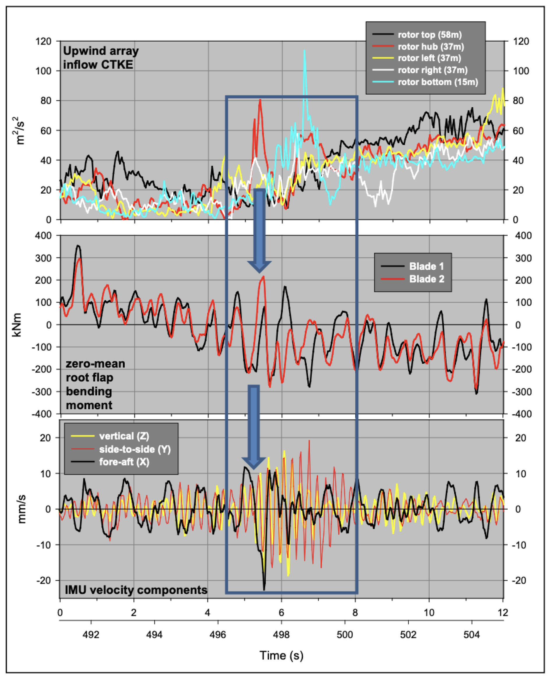
These combined effects must be taken into consideration when estimating partially waked turbine fatigue loads.

We conclude that we must adequately revise the wind turbine design and safety standards to account for increased fatigue loading in extended wind turbine clusters. The increasing wind turbine size and height require further exploration of the atmospheric flow conditions at higher elevations (100–400 m). Recent studies based on tall tower and lidar observations address this gap (e.g., Lundquist et al., 2017; Pichugina et al., 2017; Peña et al., 2021), but better characterization of shear, veer, and turbulence in this layer is still needed. The safety standards that are currently employed result from limited insight into and characterization of other turbulent flow characteristics induced by complex topography or extreme events.

8.2.1 Low-level jets

More than 20 years ago, Neil Kelley and his collaborators began investigating the impacts of LLJs on wind turbine loads. They incorporated some of the characteristics of observed LLJs into the popular turbine inflow generation code called TurbSim (Jonkman, 2009). Their findings were presented in several publications, including a comprehensive report by Kelley et al. (2004), which provides particularly insightful information. Almost a decade later, Park et al. (2014, 2015) conducted a follow-up investigation on the impacts of LLJs on wind turbine loads. Instead of using synthetically produced stochastic inflows (e.g., via TurbSim), they used inflow data generated through LES to investigate the impact of realistic inflows on various turbine loads, including the out-of-plane bending moment, which causes deformation in the direction perpendicular to the rotor plane, and the tower-top yaw moment, which causes the tower to rotate around its vertical axis. All the LES runs included dynamically evolved LLJs. Based on these LES-based inflows, Park et al. (2014, 2015) computed wind turbine loads using the FAST model. For comparative analysis, neutrally stratified inflow fields were generated using TurbSim following the prescriptions by the IEC (e.g., Kaimal spectra). The impact of LLJs and associated strong shears (both speed and directional shears) on turbine loads is evident in Fig. 16.

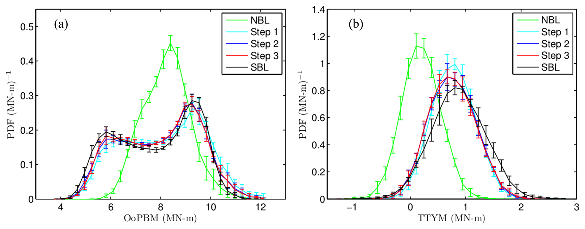
Figure 16 Probability density functions (pdf's) of simulated wind turbine loads utilizing IEC-NBL (green lines) and LES-SBL (black lines) inflows, representing the out-of-plane bending moment (OoPBM; panel a) and tower-top yaw moment (TTYM; panel b), respectively. Load calculations were performed using the FAST model on a hypothetical 5 MW turbine developed by NREL. The IEC-NBL inflows were generated using a stochastic inflow generation code called TurbSim (Jonkman, 2009). For LES-SBL inflows, a pseudo-spectral LES code employing a dynamic SGS model (Basu et al., 2008) was used to generate the inflow fields and associated LLJs. Steps 1 through 3 represent modifications of the inflow by varying wind shear (step 1), veer (step 2), and turbulence level (step 3). The hub height wind speed values from the IEC-NBL and LES-SBL inflows are closely matched (source: Park et al., 2015, published under CC BY 4.0 license).

Gutierrez et al. (2016) utilized high-frequency measurements from a 200 m tall met mast in Texas to study the impact of LLJs on wind turbine loads. Their findings indicate that LLJs caused increased static and mechanical loads and enhanced fatigue cycles. In a subsequent study, Gutierrez et al. (2017) analyzed the blade, nacelle, tower motions, tower forces, moments, and blade loads in the presence of LLJs. They concluded that negative wind shears (when the LLJ nose is below the hub height) improved the mechanical loading for the nacelle and tower and recommended using taller turbine towers to take advantage of the benefits of harvesting LLJ-enhanced energy.

Zhang et al. (2019) employed the engineering LLJ inflow model and the von Kármán spectral model as input for the FAST model to show that LLJs increase the aerodynamic loads on turbines. Gadde et al. (2021) used LES and showed that the shear causes significant azimuthal variation in the external aerodynamic blade loading, increasing fatigue loading on the turbines. Chatterjee et al. (2022) used mesoscale-driven LES coupled to an aeroelastic solver to demonstrate that the strong veer associated with LLJs significantly increases the damage equivalent hub loads and tower loads of isolated turbines and turbines placed in wind farms. In wind farms, the reduction in the LLJ strength with downstream distance in the wind farm reduces its impact. This highlights that the results obtained from analyzing the impact of LLJs on isolated turbines may not immediately apply to the entire wind farm.

8.3 Terrain effects and loads

Terrain-induced circulations can result in highly variable winds and intermittent turbulence that impact turbine performance. It is, therefore, important to characterize wind gusts in complex terrain. Kawashima and Uchida (2018) investigated the impact of terrain-induced turbulence on blade fatigue loads based on strain measurements. By combining measurements with numerical simulations, they developed a method for optimal turbine placement in complex terrain. Uchida (2018) conducted LES to analyze turbulence intensity impacting a turbine in the Atsumi wind farm. The LES output analysis confirmed a higher turbulence intensity induced by the terrain effects. Resolving the terrain-induced vortex structure that resulted in high turbulence intensity required a 5 m grid resolution. Uchida (2019) also analyzed the cause of the wind turbine blade damage accident at Shiratakiyama wind farm. This study suggested that vortex shedding from the hill located upwind from the wind farm resulted in more intense turbulence that caused blade damage. Hu et al. (2018) analyzed wind gusts in moderately complex terrain and calculated wind gust parameters and their associated parent distribution. They identified a linear relationship between turbulence intensity and gust factors. In a follow-up study, Letson et al. (2019) characterized wind gusts observed during the Perdigão field study and found that gust length scales on ridge tops scale with the height of the ridge and concluded that terrain features impact gust length scales more than their magnitude. In complex terrain, flow characteristics depend significantly on wind direction due to specific terrain and land cover features and differences in atmospheric stability. Atmospheric stability dependence on the wind direction can be particularly pronounced in coastal environments.

Field studies of turbulence effects can be complemented with wind tunnel experiments. The advantage of wind tunnel experiments is that they allow flow parameters to be varied in a controlled manner. While there are studies that replicated some of the atmospheric conditions (e.g., Chamorro and Porté-Agel, 2010), the disadvantage is that unless a wind tunnel is pressurized (Miller et al., 2019), it is not possible to achieve the high-Reynolds-number characteristic for atmospheric flows. In addition, a range of atmospheric stabilities and Coriolis effects and their consequences (e.g., veer, LLJs, AGWs) are difficult or impossible to replicate. Nevertheless, controlled experiments can yield useful insights into turbulence characteristics in a wind farm (e.g., Kozmar et al., 2018). Vanderwel et al. (2017) designed a wind tunnel experiment to study the effects of surface heterogeneities. They found that surface heterogeneities result in significant differences in the shear stress distribution, which could affect the fatigue life of turbines depending on their placement relative to these heterogeneities.

Considering that it can be expected that wind power capacity deployed in complex terrain will continue to grow in coming years, more attention is being paid to analyzing the effects of complex terrain on wind turbine loads. However, more research is required to better characterize terrain-induced turbulence, including the effects of upwind fetch. This goal can be achieved by analysis of observations from field studies complemented with extensive high-resolution numerical simulations.

8.4 Extreme events and loads

Wind engineers have studied the effects of high-impact, extreme winds on buildings, bridges, transmission towers, and other structures for decades. Numerous examples are available in several books on wind engineering (e.g., Simiu and Scanlan, 1996; Holmes, 2007, Solari, 2019). In contrast, the effects of extreme winds on wind turbines and wind farms have been reported only by a handful of papers. A small percentage of these papers documented various types of damage due to actual meteorological events; others performed idealized numerical simulations and structure load analysis.

This conclusion can be extended to wind turbine design standards, as demonstrated by Pehar et al. (2019), who analyzed the measurements of turbulence intensity during a downslope wind event and concluded that their observations do not fall within any of the turbulence classes outlined in the IEC 6100-1 standard. The relative sparsity of observations of downslope windstorms can be overcome using high-resolution, turbulence-resolving numerical simulations. However, while LES can quite accurately represent details of downslope windstorms (e.g., Juliano et al., 2024), due to computational complexity, such simulations are presently used as a research tool.

In early 2000, a typhoon made landfall on Miyakojima island, Japan. The recorded peak gust speed was 74.1 m s⁻¹. Among the six turbines present, three turbines were completely destroyed, while the remaining turbines suffered significant damage (Ishihara et al., 2005). A more recent occurrence, documented by Hawbecker et al. (2018), was a thunderstorm featuring multiple downbursts and tornadoes that swept through the Buffalo Ridge wind farm in Minnesota, USA, in 2011. The powerful wind gusts not only inflicted damage to turbine blades but also caused a turbine tower to buckle. Tornadoes ripped through Harper County, Kansas, on 19 May 2012 (source: https://www.youtube.com/watch?v=Egdtlnv6Gio, last access: 15 January 2025); five wind turbines were destroyed at a wind farm that was under construction nearby (AbuGazia et al.). In 2017, Hurricane Maria caused significant damage to 13 wind turbines at the Punta Lima wind farm in Puerto Rico. Some blades broke, and others experienced delamination (Kwasinksi et al., 2019).

There has been relatively little research into the interactions between downslope wind storms, power production, and turbine loads compared to studies of other extreme wind events. Observational studies, such as those by Sherry and Rival (2015), studied wind ramps associated with chinook winds downwind in the Canadian Rockies. One of their findings was that turbulence intensity was generally large during ramp events. Kozmar and Grisogono (2020) provided a review of the characteristics of downslope wind storms, including mountain wave overturning, quasi-periodic oscillations in wind speed, and elevated turbulence levels as a result of Kelvin–Helmholtz instabilities, which are particularly relevant for wind energy applications. They point out the need for updating engineering standards to account for large wind velocity fluctuations associated with downslope wind storms.

Turbine incidents and failures are underreported. There are only a few data mining studies of wind turbine failures and accidents based on textual analysis of news reports (e.g., Ertek and Kailas, 2021). There is a need for the creation of a comprehensive database of failures for better assessment of the impact of extreme events on individual wind turbines and wind farms and for more accurate risk assessment.

In the following subsections, we elaborate on the idealized studies that focused on downbursts and hurricanes.

8.4.1 Downbursts

Downbursts are low-level diverging outflows that can generate extreme winds when they occur (Fujita, 1985; Wakimoto, 1985). Downbursts are often associated with thunderstorms and are dominated by severe horizontal components of the wind field (see Fig. 17a and b). However, they are also accompanied by strong vertical motions at low levels. Although downbursts pose a serious threat to wind turbine structures, the IEC or other standards for wind turbine design do not describe them realistically.

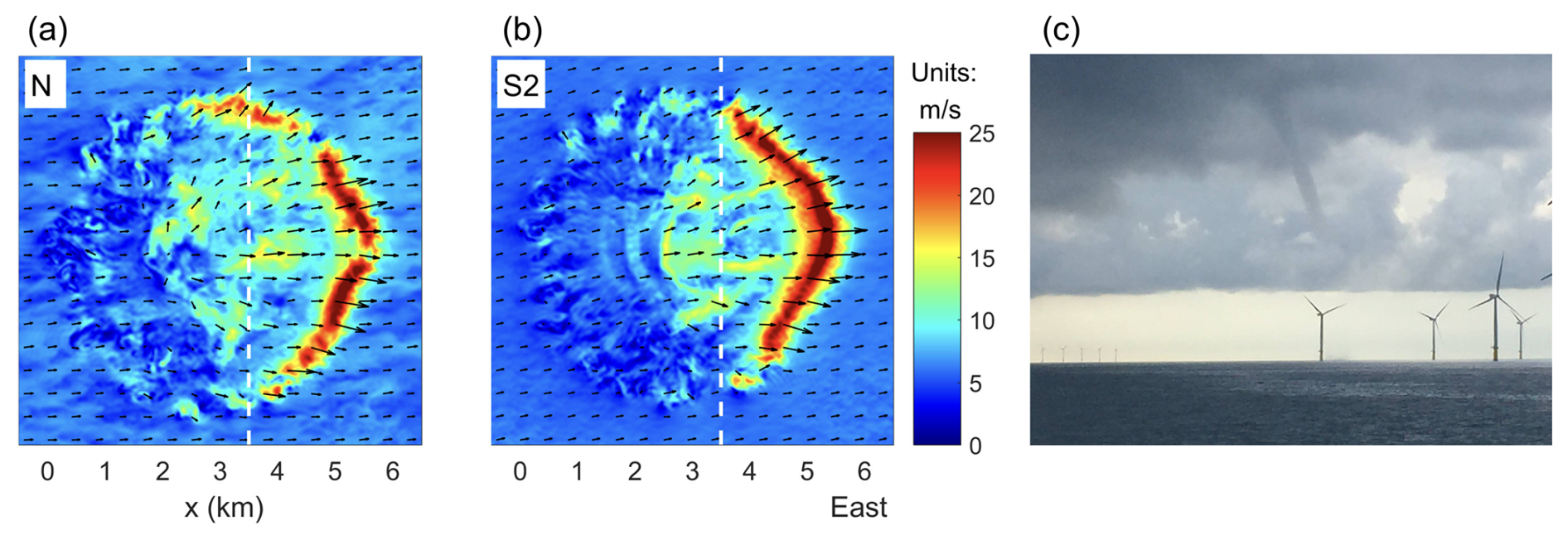
Figure 17 (a, b) Downbursts simulated by a pseudospectral LES code employing a dynamic SGS closure. The ambient turbulence condition is neutrally (left) and stably (right) stratified (source: Lu et al., 2019, published under CC BY 4.0 license). (c) A waterspout at Walney wind farms, UK, in 2015 (photo by Chris Hall).

Nguyen et al. (2011, 2013) and Nguyen and Manuel (2015a) developed engineering models for simulating velocity fields characteristic of downbursts. The velocity fields were composed of non-turbulent and turbulent parts. The non-turbulent part was generated by using simple analytical models. In contrast, a stochastic simulation with prescribed power spectral density and coherence was used for the non-turbulent part. The FAST model was used to estimate the tower and rotor loads of utility-scale wind turbines. The simulated downbursts exhibited strong surface winds coupled with rapid wind direction change. The aeroelastic simulations highlighted the need for blade pitch and nacelle yaw controls to limit turbine loads.

Lu et al. (2019) used a cooling source approach (mimicking evaporative cooling) in conjunction with LES to model downbursts. Compared to the hybrid analytical–stochastic model of Nguyen and Manuel (2015b), the LES-generated velocity fields produced more rapid changes in wind speed and direction. These differences were found to have significant influences on extreme and fatigue loads using the aeroelastic simulation tool FAST V8 (Jonkman and Jonkman, 2016).

Waterspouts have some morphological similarities to tornadoes and downbursts. Hence, they may induce damage to offshore or coastal turbines. At this point, we are not aware of any such incidents. However, some online images document the occurrence of waterspouts near wind farms; see an example in Fig. 17c. As the worldwide growth of offshore wind energy continues, the threats of waterspouts will likely increase at some offshore locations (e.g., the North Sea).

8.4.2 Tropical and extratropical cyclones

Tropical cyclones (TCs), defined as warm-core synoptic-scale cyclones originating over tropical or subtropical waters with organized deep convection and a closed surface wind circulation, can present a damaging series of loads to impacted wind turbines. When the 1 min average wind exceeds 33 m s⁻¹, the TC becomes known as a hurricane or typhoon. Due to significant turbulence levels and associated wind gusts, tropical cyclones can result in turbine loads outside the IEC 61400-3 design standard (Kapoor et al., 2020). In Annex J of IEC 61400-1 (2019), tropical cyclones are addressed based on random sampling from statistical distributions of relevant hurricane parameters from historical track data. While this enables a level of confidence in the statistical prediction of extreme wind for wind turbine design, considering the potential impact, the standard should be continuously evaluated based on available observations and high-resolution simulations.

A series of studies that analyzed data produced from an LES of a category five hurricane showed that the design standards are inadequate for such a strong hurricane. Worsnop et al. (2017a) showed that this simulation with the Cloud Model 1 (Bryan and Rotunno, 2009, CM1;) effectively models Hurricane Isabel in terms of mean wind speeds, wind speed variances, and power spectra. Further work (Worsnop et al., 2017a) demonstrated that the greatest wind speeds occur in the eyewall, with peak 3 s gusts exceeding 70 m s⁻¹ and up to 100 m s⁻¹, which would cause extreme aerodynamic and structural loading that could lead to damage or failure, agreeing with analysis of dropsonde wind speeds (Stern et al., 2016). They showed that gust factors can reach 1.7 at the eye–eyewall interface, well beyond what has been considered previously. Rapid changes in wind direction and wind veer during hurricanes can also be quite problematic, increasing both blade and tower loads (Kapoor et al., 2020). Additionally, observational studies with dropsondes (Stern et al., 2016) reveal extreme low-level updrafts in strong hurricanes, with the azimuthal distribution being related to shear orientation and storm movement. Sanchez Gomez et al. (2023) suggested that the IEC standards may be insufficient for defining turbines that could withstand the strongest TCs. This is also the message from Müller et al. (2024b, a), particularly on typhoon cases.

Wang et al. (2024a) presented a summary of a workshop conveyed to address the needs and challenges related observations, modeling, risk assessment, and climate change impacts of tropical and extratropical cyclones on offshore wind energy in the US. The workshop highlighted the need for enhanced observational capabilities, coupled atmosphere–wave–ocean modeling, bridging the gap between temporal and spatial scales of weather forecasting and wind turbine operation, and development of effective risk assessment frameworks. A review of relevant work that forms the background for further study appears in Wang et al. (2024b).

Extratropical cyclones, such as northeasters along the East Coast of the US, develop when cold and warm air collide, forming a front and resulting in baroclinic instability due to an imbalance in the pressure and density levels of a fluid. Maximum wind speed in extratropical cyclones can reach the same levels as in tropical cyclones. As offshore wind energy is being deployed along the Atlantic Coast of the US, there is a need to better characterize how extratropical cyclones could impact wind farms.

9 Recommendations

The projected growth of worldwide wind energy capacity makes the need for better characterization of atmospheric boundary layer wind and turbulence more pressing. The growth of wind energy capacity will inevitably lead to the deployment of wind farms in complex terrain and offshore environments where there is insufficient data and understanding about wind and turbulence characteristics. The development of increasingly large utility-scale wind turbines introduces new design challenges. These challenges require a more robust characterization of turbulent flow across the entire rotor span, particularly in regions that may extend above a shallow ABL. Therefore, the projected wind energy deployment goals will require research efforts informing new design standards that would ensure the efficiency and reliability of wind turbines and wind farms. Some main knowledge gaps that must be addressed to achieve the projected goals are outlined below.

• Mesoscale-modulated turbulence associated with low-level jets, mesoscale convective circulations (convective cells and convective rolls), and gravity waves is observed onshore and offshore. The impact on potential wind farm production or turbine loading is less clear, aside from a few isolated examples. A thorough analysis of more wind farm production data is required, coupled with detailed measurement campaigns using remote sensing instruments such as Doppler lidar and numerical modeling to pin down the impact of these different phenomena, particularly the impact of the different time and length scales of the turbulence associated with such mesoscale structures.

• The characterization and quantification of the effects of atmospheric stability, non-homogeneity, and coherent structures on turbulence non-stationarity, coherence, and length scales and their impacts on aerodynamic performance and wind turbine loads are still lacking. More specialized in-field measurements at the blade level are required to understand these impacts fully.

• Presently, the majority of turbulence characterization and its impacts on power production and loads are based on the equilibrium assumption that turbulence production and dissipation are balanced. However, under dynamically evolving atmospheric conditions, equilibrium is not achieved. Therefore, there is a need to observe and synthesize the effects of non-equilibrium turbulent flows, including intermittent turbulence, on the high-frequency fluctuations of power and loads.

• Improved characterization of extreme wind and ocean conditions, including those associated with hurricanes and tropical cyclones, are needed. Values of extreme wind speed and associated gusts and turbulence levels are often beyond the recommended ones in the IEC 61400-1 (2019) standard. An important reason for this is the current trend of growing hub heights of modern-day turbines (the hub height is used as a reference in IEC 61400-1 (2019)) and hence wind speed. Research on the structures of hurricane boundary layers still reveals surprising results, as mentioned in Sect. 8.5.2.

• The frequency and magnitude of extreme events will likely be different in future climates than what is observed today. Additional research is needed to understand how atmospheric and oceanic conditions will change over the next several decades and beyond to better inform turbine design. For example, statistical distributions of key hurricane parameters (for example, occurrence rates, geostrophic shear, radius of maximum wind speed, and maximum sustained wind speed) in future climates are needed.

• The community needs more validation data to increase our understanding and to evaluate our models. For comprehensive model validation, there is a particular need for simultaneous observation of environmental conditions, details of the wind farm operation, and the interactions between the two.

• Most of the field studies described in the literature are episodic and focused on process studies. There is a need for measurements and analysis over an annual cycle, or at least several seasons, to better understand the environment in which wind turbines operate. These studies should be conducted in areas with different topographies and land use/land cover. Considering that the lifetime of a wind turbine should be 20 or more years, there is a need for long-term measurement of turbulence.

• Continuing development of model benchmarks focusing on tests that specifically assess turbulence characterization is needed. An example is the recently initiated International Energy Agency (IEA) Wind Task 57 – Joint Assessment of Models (JAM), which is a benchmark successor to Wakebench.

• Currently, there are several advanced research tools and computer models under development that utilize advanced computational platforms and algorithms (e.g., GPUs, accelerators, and machine learning) and provide the ability to conduct turbulence-resolving simulations of unprecedented fidelity. There is an opportunity to transfer some of these tools from research to applications.

As outlined above, facilitating continued growth of wind energy capacity requires better characterization of turbulence in the ABL under a wider range of large-scale atmospheric forcing, including non-stationary conditions, over non-homogeneous terrain, and when turbulence is out of equilibrium. Addressing the gaps in our knowledge would contribute not only to a better understanding of turbulent processes in the ABL but also to wider deployment of wind energy.