Power curve and wake analyses of the Vestas multi-rotor demonstrator

Numerical simulations of the Vestas multi-rotor demonstrator (4R-V29) are compared with field measurements of power performance and remote sensing measurements of the wake deficit from a short-range WindScanner lidar system. The simulations predict a gain of 0 %–2 % in power due to the rotor interaction at below rated wind speeds. The power curve measurements also show that the rotor interaction increases the power performance below the rated wind speed by 1.8 %, which can result in a 1.5 % increase in the annual energy production. The wake measurements and numerical simulations show four distinct wake deficits in the near wake, which merge into a single-wake structure further downstream. Numerical simulations also show that the wake recovery distance of a simplified 4R-V29 wind turbine is 1.03–1.44 D_eq shorter than for an equivalent single-rotor wind turbine with a rotor diameter D_eq. In addition, the numerical simulations show that the added wake turbulence of the simplified 4R-V29 wind turbine is lower in the far wake compared with the equivalent single-rotor wind turbine. The faster wake recovery and lower far-wake turbulence of such a multi-rotor wind turbine has the potential to reduce the wind turbine spacing within a wind farm while providing the same production output.

1 Introduction

Over the past few decades, the rated power of wind turbines has been increased by upscaling the traditional concept of a horizontal axis wind turbine with a single three-bladed rotor. It is expected that this trend will continue for offshore wind turbines, although the problems that arise from realizing large wind turbine blades (> 100 m) are not trivial to solve (Jensen et al., 2017). An alternative way to increase the power output of a wind turbine is the multi-rotor concept, where a single wind turbine is equipped with multiple rotors. From a cost point of view, it can be cheaper to produce a multi-megawatt wind turbine with several rotors consisting of relatively small blades that are already mass produced compared with a single-rotor wind turbine with newly designed large blades (Jamieson et al., 2014). In addition, small blades are easier to transport than large blades, which makes a multi-rotor concept interesting for locations where infrastructure is a limiting factor. However, multi-rotor wind turbines also have disadvantages; for example, a more complex tower is required and the number of components is higher compared with single-rotor wind turbines.

The multi-rotor concept is an old idea that dates back to the start of 19th century. Between 1900 and 1910, a Danish water management wind mill, was upgraded to a twin-rotor wind mill (Holst, 1923). Around the 1930s, Honnef (1932) introduced the multi-rotor concept for an electricity generating wind turbine, as discussed by Hau (2013). In the late 20th century, the Dutch company Lagerwey built and operated several multi-rotor wind turbine concepts based on two, four and six two-bladed rotors (Jamieson, 2011). In April 2016, Vestas Wind Energy Systems A/S built a multi-rotor wind turbine demonstrator at the Risø Campus of the Technical University of Denmark. This multi-rotor wind turbine, hereafter referred to as the 4R-V29 wind turbine, consists of four V29-225 kW rotors, which are arranged as a bottom and top pair. The 4R-V29 wind turbine operated for almost 3 years and was decommissioned in December 2018. In the present article, we investigate the power performance and wake interaction of the 4R-V29 wind turbine using field measurements and numerical simulations.

The tip clearances between the rotors in multi-rotor wind turbines are typically much smaller than a single-rotor diameter, and several authors have shown that the operating rotors strongly interact with each other. Chasapogiannis et al. (2014) and Jamieson et al. (2014) performed numerical simulations of closely spaced rotors positioned in a honeycomb layout with a tip clearance of 5 % of the (single) rotor diameter. Chasapogiannis et al. (2014) simulated seven 2 MW rotors using computational fluid dynamics and vortex models, and they calculated an increase in power and thrust of about 3 % and 1.5 %, respectively, compared with seven non-interacting single rotors. In addition, Chasapogiannis et al. (2014) found that the seven individual single wakes merge into a single-wake structure at a downstream distance equal to or further than two rotor diameters. Jamieson et al. (2014) simulated a 20 MW multi-rotor wind turbine consisting of 45 444 kW rotors. They argued that wind turbine loads are reduced compared with a single-rotor 20 MW wind turbine because of load-averaging effects when using 45 small rotors; furthermore, they reported that the power performance is increased due to rotor interactions, and the fact that smaller wind turbines can respond faster to wind speed variations. More recently, Jensen et al. (2017) reported an 8 % power increase for the same multi-rotor wind turbine using a smaller tip clearance of 2.5 % or the rotor diameter. Nishino and Draper (2015) employed Reynolds-averaged Navier–Stokes (RANS) simulations of a horizontal array of actuator discs (AD) with a tip clearance of 50 % of the rotor diameter and an optimal thrust coefficient. They found an increase in the wind farm power coefficient, based on the axial induction of the ADs (up to 5 %), when increasing the number of ADs from one to nine. Nishino and Draper (2015) also simulated an infinite array of ADs, but the domain blockage ratio for this case was too high (2 %) to obtain a valid result, as also discussed in Sect. 3.2.2 of the present article.

Ghaisas et al. (2018) employed large-eddy simulations (LES) and two engineering wake models to show that a general multi-rotor wind turbine consisting of four rotors has a faster wake recovery and lower turbulent kinetic energy in the wake compared with a single rotor with an equivalent rotor area. They argued that the faster wake recovery is a result of a larger entrainment, as the ratio of the rotor perimeter and the rotor swept area is twice as high for their multi-rotor turbine compared with a single-rotor turbine. In the same work, it was also shown that different tip clearances in the range of zero to two rotor diameters hardly effect the wake recovery of the multi-rotor wind turbine, whereas the turbulent kinetic energy in the far wake varies, although it is always less than the turbulent kinetic energy in the far wake of a single rotor. Finally, it was shown that the power deficit and the added turbulent kinetic energy in the wake of a row of five multi-rotor wind turbines is less than for a row of five single-rotor wind turbines. These results suggest that a wind farm of multi-rotors has lower power losses and fatigue loads due to wakes than a wind farm of single-rotor wind turbines. In the present article, we attempt to confirm the results of Ghaisas et al. (2018) for the 4R-V29 wind turbine using different models and levels of ambient turbulence.

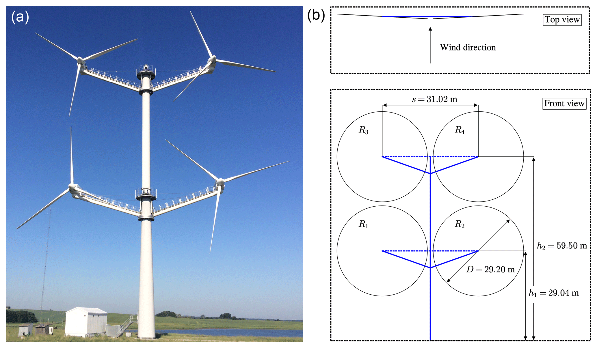
Figure 1 (a) The 4R-V29 wind turbine located at the Risø Campus. (b) Sketch of the 4R-V29 wind turbine, including dimensions and rotor definitions, shown using a top and front view.

2 Field measurements

2.1 Description of the 4R-V29 wind turbine

Figure 1 depicts the 4R-V29 wind turbine located at the Risø Campus of the Technical University of Denmark and a corresponding sketch including dimensions and rotor definitions. The hub height of the bottom rotor pair (R₁ and R₂) and the top rotor pair (R₃ and R₄) are 29.04 and 59.50 m, respectively, which gives an average hub height of 44.27 m. The horizontal distance between the nacelles for both pairs is 31.02 m. The rotors are equipped with 13 m (V27) blades, where the blade root is extended by 1.6 m, resulting in a rotor diameter of 29.2 m. The rotor tilt angles and the cone angles (the angle between the individual rotor plane and its blade axis) are all zero. To increase the horizontal distance between the rotors (tip clearance), the 4R-V29 has a toe-out angle of 3^∘, as depicted in the top view sketch in Fig. 1. This means that the left rotors (R₁ and R₃) and the right rotors (R₂ and R₄) are yawed by +3 and −3^∘, respectively. (A positive yaw angle is a clockwise rotation as seen from above.) The horizontal and vertical tip clearances are 1.86 and 1.26 m, or 6.4 % and 4.3 % of the single-rotor diameter, respectively, which is close to the 5 % used in simulations performed by Chasapogiannis et al. (2014) and Jamieson et al. (2014). It is possible to yaw the bottom and top pairs independently of each other, which could be beneficial in atmospheric conditions where a strong wind veer is present (i.e., a stable atmospheric boundary layer).

2.2 Power curve measurements

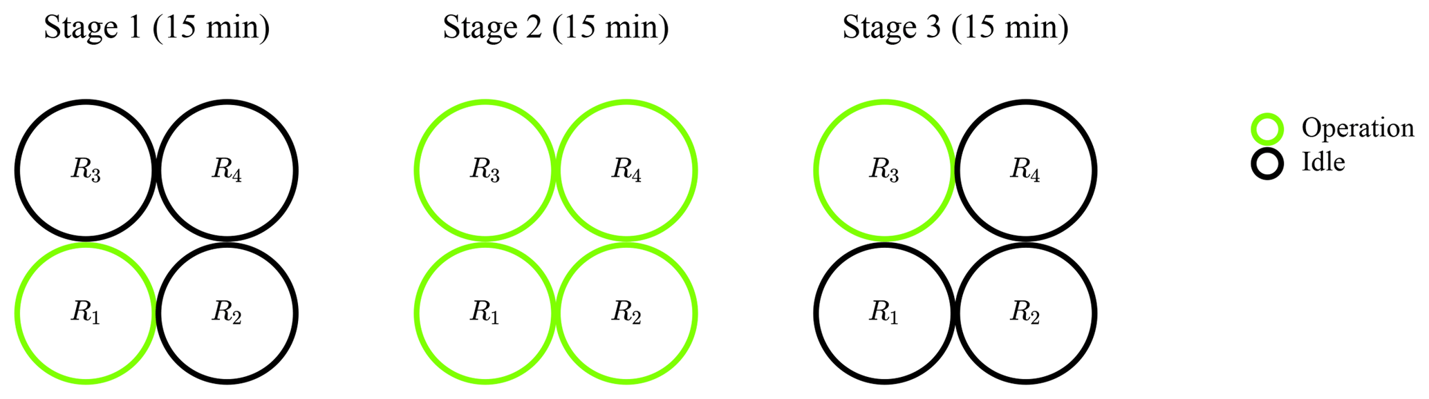
Power curve measurements of the 4R-V29 wind turbine were carried out to quantify the effect of the rotor interaction on the power performance. For this purpose, a test cycle of three stages was run repetitively, as illustrated in Fig. 2. During stages 1 and 3, only rotors R₁ and R₃ were in operation, respectively, whereas the other rotors were in idle. During Stage 2, all rotors were in operation. We used two single-rotor operation stages to account for the effect of the shear. Each stage was run for 15 min and was post-processed to 10 min data samples via the removal of start up and shutdown periods between the stages. By toggling the stages at every 15 min, we minimized differences in environmental conditions between the three data sets (one data set per stage).

Figure 2 Test cycle of power curve measurements of the 4R-V29 wind turbine.

The reference wind speed is measured using a commercial dual-mode continuous-wave lidar, ZephIR 300, manufactured by ZephIR (UK) (Medley et al., 2014). The lidar is mounted on the top platform of the 4R-V29 wind turbine at height of 60 m, as depicted in Fig. 3a. It measures the upstream wind speed at 146 m (5 D) and 300 m (≈10.3 D), at a height of 44.3 m, as shown in Fig. 3b. We chose to use the lidar measurements of the reference wind speed at 146 m because the lidar measurements at 300 m have a lower data availability and a higher volume averaging. In order to capture the wind speed at a hub height of 44.3 m, the instrument is configured with a tilt angle of −7^∘, such that the center of the scan is directed towards the desired measurement height, as illustrated in Fig. 3. A horizontal pair of measurements at this height are used to determine the wind speed and yaw misalignment, using a pair-derived algorithm. The lidar measurements are corrected in real time for tilt variations due to the tower deflection. A sample, measured every 1 s (1 Hz), is corrected for the difference in the induction zone for when only one or all four rotors are in operation, as discussed in Appendix A. The corrected data samples are averaged over 10 min and then binned in wind speed intervals of 0.5 m s⁻¹. It should be noted that applying the induction correction after the 10 min averaging did not make a difference for the final power curve.

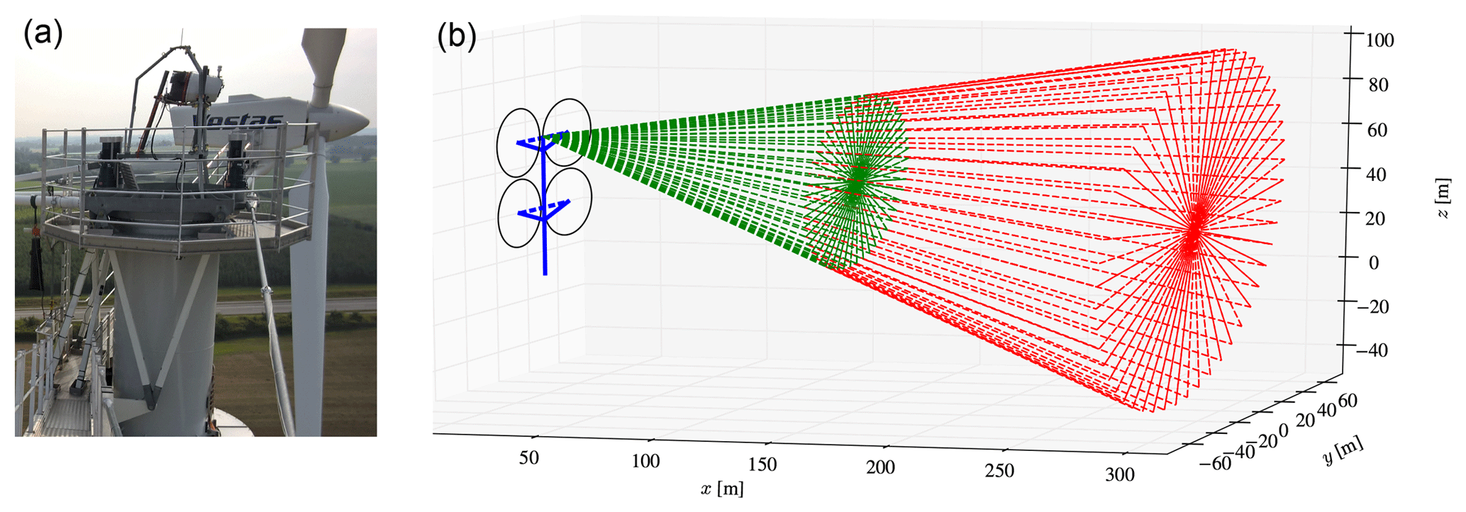
Figure 3 (a) The ZephIR Z300 placement on the 4R-V29 wind turbine. (b) Scanning cone for x=146 m (green) and x=300 m (red).

The total number of available measurement cycles is depicted in Fig. 4b and corresponds to 549 10 min data samples or approximately 91.5 h for each stage between wind speeds of 4 and 14 m s⁻¹. The total amount of data per stage is about half of the minimal requirement as defined in the international standard (IEC, 2005), where a power curve database should include at least 180 h of data and a minimal of 30 min per binned wind speed. In addition, there is not much data available above the rated wind speed. As a result, the standard error of the mean power in a bin is high, as shown by the error bars in the power curves of Fig. 4a. These two power curves represent the sum of power from rotors R₁ and R₃ of stages 1 and 3, and the sum of power from rotors R₁ and R₃ of Stage 2, both multiplied by a factor of 2. The relative difference between the power curves is discussed in Sect. 4.2. The power curve measurements are filtered for events where a rotor (that is planned to operate) is not in full operation. During the power curve measurements, the neighboring V27 and Nordtank (NTK) wind turbines were not in operation (see Fig. 5). To avoid the influence of the other neighboring wind turbines and flow disturbance from a motorway, the power measurements are filtered for a wind direction sector 180–330^∘, which represents an inflow from the fjord (see Fig. 5). It should be mentioned that the wind turbine test site at the Risø Campus is not flat. The influence of this is minimized by adjusting the lidar configured height to match the height difference upstream, although this could slightly influence the power curve measurements. In addition, the power curve measurements are not filtered for turbulence intensity and atmospheric stability, as the amount of data remaining after filtering would be too small. However, the measurements are filtered for normalized mean fit residuals below 4 %, which removes data samples with a high complexity of incoming flow.

Figure 4 (a) Measured electric power of 2(R₁+R₃) from the 4R-V29 wind turbine as a function of the free-stream velocity at a height of 44.27 m for all rotors and single rotors in operation. Error bars represents the standard error of the mean power. (b) Number of test cycles.

2.3 Wake measurements

The wake of the 4R-V29 turbine has been measured by three ground based short-range WindScanners (Mikkelsen et al., 2017; Yazicioglu et al., 2016) during two separate measurement campaigns, referred as the near-wake and the far-wake campaigns. The measurement setup is shown in Fig. 5. The three WindScanners measure the wake deficit by synchronously altering the line-of-sight azimuth and elevation of each individual unit. In the near-wake campaign, the WindScanners scanned three cross planes located at 0.5 D, 1 D and 2 D downstream. In addition, a horizontal line at the lower hub height 1 D downstream was rapidly scanned at about 1 Hz. Each cross plane/line is scanned for 10 min, before moving on to the next, which means that every 40 min a complete set of three cross planes is available. The data are stored in 1 min files and the 10 min scans are post-processed for minutes without scan plane transitions, rendering 8 min means. The far-wake campaign consists of only one cross plane scanned at 5.5 D downstream. It is not possible to scan further downstream due to the presence of a highway and surrounding trees located 170–200 m downstream of the 4R-V29 wind turbine for a wind direction of 280^∘. The WindScanners are positioned in between the near- and far-wake scanning distances. The selected WindScanner positions allow near- and far-wake measurements to be monitored by turning the “pointing direction” toward and away from the 4R-V29 wind turbine, respectively. This configuration allows for the estimation of the two components of the horizontal wind vector by assuming that the vertical component is equal to zero. During the wake measurements, the neighboring Nordtank (NTK) and V27 wind turbines were not in operation.

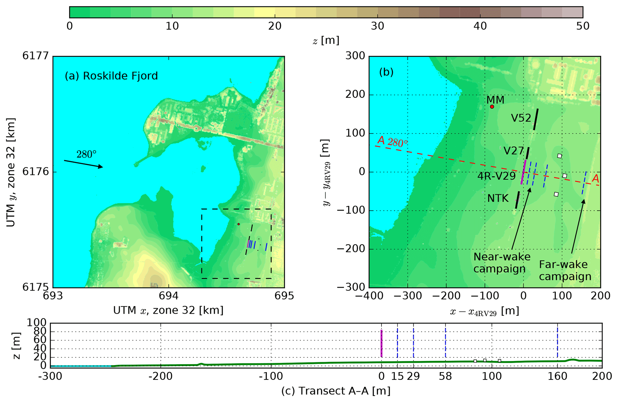
Figure 5 Topography around the 4R-V29 wind turbine, and an overview of wake measurements. Panel (b) is a zoomed-in section of panel (a). (c) The terrain height along transect A–A. The locations of three WindScanners are shown as white squares, the scanning locations are shown as blue dashed lines, MM is the met mast, and V52, V29 and NTK are neighboring wind turbines.

Figure 6 summarizes the atmospheric conditions during the near- and far-wake measurements, as measured at the met mast depicted in Fig. 5. The met mast is equipped with pairs of cup and sonic anemometers located at five heights: 18, 31, 44, 57 and 70 m. The wind speed and wind direction are taken from a cup and a sonic anemometer, respectively, both located at a height of 44 m, which is close to the average hub height of the 4R-V29 wind turbine. The turbulence intensity and the atmospheric stability in terms of a Monin–Obukhov length L_MO are measured by sonic anemometers located at heights of 44 and 18 m, respectively.

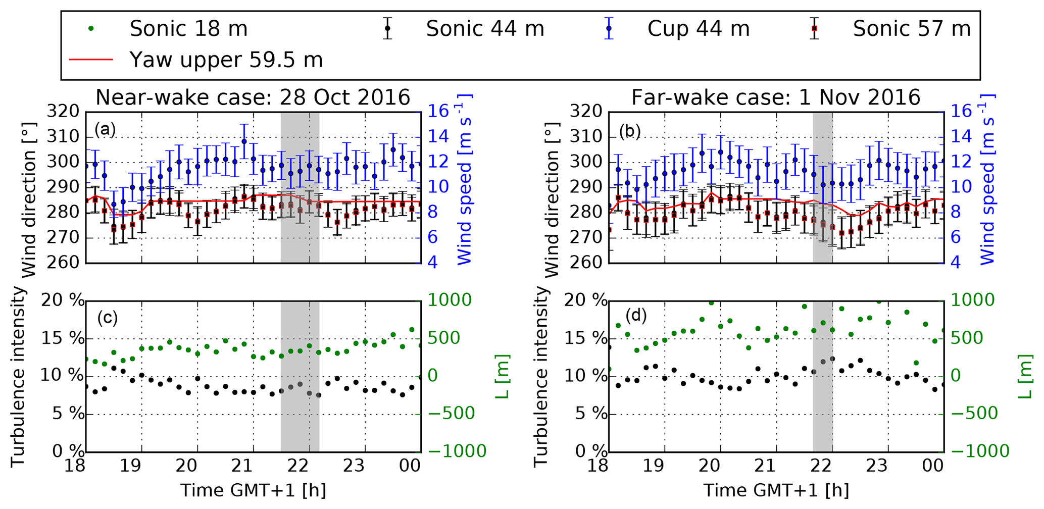
Figure 6 Atmospheric conditions during the near- and far-wake measurements as measured at the V52 met mast. (a, b) Wind direction in addition to wind speed and yaw angle of the upper platform. (c, d) Total turbulence intensity and Monin–Obukhov length. Error bars represent the standard error of the mean. The gray areas depict the time of the chosen measurements.

A near-wake case is selected from three consecutive post-processed scans measured between 21:36 and 22:03 GMT+1 on 28 October 2016. A far-wake case is taken from one post-processed scan measured between 21:45 and 21:53 GMT+1 on 1 November 2016. During these periods, the atmospheric stability is near-neutral (L_MO=340 m) and neutral (L_MO=661 m). The wind direction in both cases is close to 280^∘, and the yaw offset with respect to the upper platform is 3.4 and 8.2^∘ for the near- and far-wake cases, respectively. The atmospheric conditions of the two cases are listed in Table 1, and are used as input for the numerical simulations. Note that the simulations only consider neutral atmospheric stability.

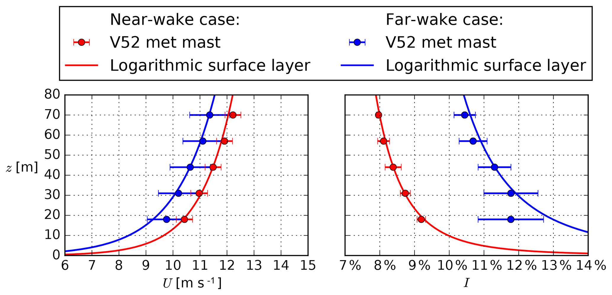
Figure 7 Profiles of wind speed and turbulence intensity measured at the met mast and corresponding logarithmic surface layer using U_ref and I_ref from Table 1 for the near- and far-wake measurement cases. Error bars represent the standard error of the mean.

The wind speed and total turbulence intensity profiles measured at the met mast during the near- and far-wake case recordings are depicted in Fig. 7. The wind speed and turbulence intensity at 44 m (U_ref and I_ref) are used to determine the neutral logarithmic inflow profiles defined by z₀ and u_* following Eq. (2). The results are listed in Table 1. The far-wake profile deviates from a logarithmic profile at a height of 18 m, which could be related to the upstream fjord-land roughness changes, as shown in Fig. 5, although this deviation is not observed in the near-wake case inflow profile.

Spectra of 35 Hz wind velocity data measured by the sonic anemometer at 44 m are used to fit Mann turbulence spectra (Mann, 1994) utilizing three parameters: αϵ^⅔, L and Γ. When these parameters are used to generate a Mann turbulence box, which is employed as inflow turbulence for the MIRAS-FLEX5 and EllipSys3D LES-AL-FLEX5 simulations (Sect. 3), the resulting turbulence intensity in the Mann turbulence box is lower than the measured value at the sonic anemometer, which is not fully understood. The problem is circumvented by using an αϵ^⅔ that is about twice as large as original fitted value. The final values of αϵ^⅔, L and Γ are listed in Table 1. Note that the stream-wise dimension of the Mann turbulence box is chosen to fit an entire measurement case (40 min) using ${\mathrm{2}}^{\mathrm{14}}\times {\mathrm{2}}^{\mathrm{7}}\times {\mathrm{2}}^{\mathrm{7}}$ points in the stream-wise and cross direction, respectively, with a spacing of 2 m in all directions.

Table 1 Summary of test cases based on wake measurements and corresponding input parameters for numerical computations.

3 Simulation methodology

Four different simulations tools are employed to model the 4R-V29 wind turbine: Fuga, EllipSys3D RANS-AD, MIRAS-FLEX5 and EllipSys3D LES-AL-FLEX5. The simulation methodology for each model, ranked from the lowest to highest model fidelity, is described in the following sections. Note that a high model fidelity corresponds to an intended high accuracy at the price of a high computational cost, although good model performance is not guaranteed. All simulations that are used to model the 4R-V29 wind turbine only assume a neutral atmospheric surface layer inflow. In addition, only flat terrain with a homogeneous roughness length is modeled; hence, the effects of the fjord-land roughness change and sloping terrain are neglected.

3.1 Fuga

Fuga is a fast linearized RANS model developed by Ott et al. (2011). Fuga models a single wind turbine wake as a linear perturbation of an atmospheric surface layer. In the present setup, a thrust force is modeled that is distributed uniformly over the rotor-swept area. The forces are smeared out using a two-dimensional Gaussian filter with standard deviations of D∕4 and D∕16 in the stream-wise and cross directions. The turbulence is defined using the eddy viscosity of an atmospheric surface layer, which means that a wind turbine wake does not affect the turbulent mixing. The resulting equations are transformed to wave-number space in the horizontal directions to obtain a set of mixed spectral ordinary differential equations. As these equations are very stiff, a novel numerical solving method was developed by Ott et al. (2011). The linearity of the model allows for the superposition of single wakes, and is also applicable in multi-rotor configurations.

3.2 EllipSys3D RANS-AD

EllipSys3D is an incompressible finite volume flow solver, initially developed by Sørensen (1994) and Michelsen (1992), which incorporates both RANS and LES models, and has different methods of representing a wind turbine. In this section, the RANS-AD method is discussed. The Navier–Stokes equations are solved using the SIMPLE algorithm (Patankar and Spalding, 1972), and the convective terms are discretized using a QUICK scheme (Leonard, 1979). The wind turbine rotors are represented by actuator discs (ADs) based on airfoil data as presented in Réthoré et al. (2014). The RANS-AD model can only model stiff blades. The tip correction of Pirrung and van der Laan (2018) is applied (with a constant of c₂=29), which is an improvement of the tip correction of Shen et al. (2005). This modified tip correction models the induced drag due to the tip vortex, which leads to a stronger tip loss effect on the in-plane forces than on the out-of-plane forces. The RANS-AD model can be employed to model two different flow cases, a uniform inflow and a neutral atmospheric surface layer, which are described in the following sections (Sects. 3.2.1 and 3.2.2). The uniform inflow case is used to validate the AD model of a single V29 rotor with the results of two blade element moment codes. The neutral atmospheric surface layer flow case is used to simulate the 4R-V29 wind turbine.

3.2.1 Uniform inflow case

For the uniform inflow case, the numerical setup is fully described in Pirrung and van der Laan (2018). The uniform grid spacing around the AD is set to D∕20, which is fine enough to estimate C_T and C_P within a discretization error of 0.3 % following a previously performed grid refinement (Pirrung and van der Laan, 2018).

3.2.2 Atmospheric surface layer flow case

For the atmospheric surface layer flow case, the $k-\mathit{\epsilon }-f_{\text{P}}$ model from van der Laan et al. (2015) is employed, which is a modified k−ε model developed to simulate wind turbine wakes in atmospheric turbulence. A typical numerical domain for ADs in flat terrain and corresponding boundary conditions are employed as described in van der Laan et al. (2015). In the present work, a finer spacing of D∕20 is applied (in previous work from van der Laan et al. (2015) a spacing of D∕10 was used), and a larger uniformly spaced wake domain is used: 15 D × 5 D × 4 D (stream-wise, lateral and vertical directions), where D is a single-rotor diameter, and the 4R-V29 wind turbine is placed at 3 D downstream from the start of the wake domain. In addition, a larger outer domain is used – 116 D × 105 D × 50 D – such that the blockage effects are negligible (blockage ratio: $\mathit{\pi }/(\mathrm{105}\times \mathrm{50})=\mathrm{0.06}\mathit{\%}$). In the RANS simulations, we observed that a blockage ratio of 1 % for the 4R-V29 wind turbine is not small enough when comparing the simulated power of the 4R-V29 wind turbine with a single V29 rotor using the same domain. This is because the blockage ratio of the single V29 rotor simulation is 4 times lower than the 4R-V29 wind turbine simulation, and one would include a false gain in power for the 4R-V29 wind turbine that is caused by the difference in the blockage ratio between the V29 and 4R-V29 wind turbine RANS simulations.

The inflow conditions represent a neutral atmospheric surface layer that is in balance with the domain (without the ADs):

$$\begin{array}{ll}{\displaystyle }& {\displaystyle }U={\displaystyle \frac{u_{*}}{\mathit{\kappa }}}\ln \left({\displaystyle \frac{z+z_{\mathrm{0}}}{z_{\mathrm{0}}}}\right),\\ \text{(1)}& {\displaystyle }& {\displaystyle }k={\displaystyle \frac{u_{*}^{\mathrm{2}}}{\sqrt{C_{\mathit{\mu }}}}},{\displaystyle }& {\displaystyle }\mathit{\epsilon }={\displaystyle \frac{u_{*}^{\mathrm{3}}}{\mathit{\kappa }\left(z+z_{\mathrm{0}}\right)}},\end{array}$$

where U is the stream-wise velocity, u_* is the friction velocity, κ=0.4 is the Von Kármán constant, z is the height, z₀ is the roughness length, k is the turbulent kinetic energy, C_μ=0.03 the eddy viscosity coefficient and ε is the turbulent dissipation. The friction velocity and the roughness height can be set using a reference velocity U_ref and a reference (total) turbulence intensity $I_{\mathrm{ref}}=\sqrt{\frac{\mathrm{2}}{\mathrm{3}}k}/U_{\mathrm{ref}}$, for a reference height z_ref:

$$\begin{array}{ll}\text{(2)}& {\displaystyle }& {\displaystyle }{u}_{*}=U_{\mathrm{ref}}{I}_{\mathrm{ref}}{\displaystyle \frac{C_{\mathit{\mu }}^{\mathrm{1}/\mathrm{4}}}{\sqrt{\mathrm{2}/\mathrm{3}}}},{\displaystyle }& {\displaystyle }{z}_{\mathrm{0}}={\displaystyle \frac{z_{\mathrm{ref}}}{\exp \left(\frac{\mathit{\kappa }\sqrt{\mathrm{2}/\mathrm{3}}}{I_{\mathrm{ref}}{C}_{\mathit{\mu }}^{\mathrm{1}/\mathrm{4}}}\right)-\mathrm{1}}}\end{array}$$

The shear exponent from the power law ($U=U_{\mathrm{ref}}(z/z_{\mathrm{ref}}{)}^{\mathit{\alpha }}$) can be expressed by setting the shear at the reference height ($\partial U/\partial z{|}_{z_{\mathrm{ref}}}$) from the power law equal to that from the logarithmic profile and substituting Eq. (2):

$$\begin{array}{ll}\text{(3)}& {\displaystyle }\mathit{\alpha }& {\displaystyle }={\displaystyle \frac{u_{*}}{\mathit{\kappa }{U}_{\mathrm{ref}}}}{\displaystyle \frac{z_{\mathrm{ref}}}{(z_{\mathrm{ref}}+z_{\mathrm{0}})}}{\displaystyle }& {\displaystyle }=I_{\mathrm{ref}}{\displaystyle \frac{C_{\mathit{\mu }}^{\mathrm{1}/\mathrm{4}}}{\mathit{\kappa }\sqrt{\frac{\mathrm{2}}{\mathrm{3}}}}}\left[\mathrm{1}-\exp \left(-{\displaystyle \frac{\mathit{\kappa }\sqrt{\frac{\mathrm{2}}{\mathrm{3}}}}{I_{\mathrm{ref}}{C}_{\mathit{\mu }}^{\mathrm{1}/\mathrm{4}}}}\right)\right]\\ {\displaystyle }& {\displaystyle }=\mathrm{1.274}{I}_{\mathrm{ref}}+\mathcal{O}\left(I_{\mathrm{ref}}^{\mathrm{2}}\right)\end{array}$$

Note that the power law is not used in the simulations; however, the relation in Eq. (3) is employed to discuss the simulations in Sect. 4.1.

3.3 MIRAS-FLEX5

The in-house solver MIRAS (Method for Interactive Rotor Aerodynamic Simulations) is a multi-fidelity computational vortex model for predicting the aerodynamic behavior of wind turbines and the corresponding wakes. It has been developed at the Technical University of Denmark over the last decade, and it has been extensively validated for small to large wind turbine rotors by Ramos-García et al. (2014a, b, 2017). The turbine aeroelastic behavior is modeled by using the MIRAS-FLEX5 aeroelastic coupling developed by Sessarego et al. (2017). FLEX5 is an aeroelastic tool developed by Øye (1996), which gives loads and deflections.

In the present study, a lifting line technique is employed as the blade aerodynamic model. The blade bound circulation is modeled by a vortex line, located at the blade quarter-chord and subdivided into vortex segments. The vorticity is released into the flow by a row of vortex filaments following the chord direction (shed vorticity, which accounts for the released vorticity due to the time variation of the bound vortex) and a row of filaments perpendicular to the chord direction (trailing vorticity, which accounts for the vorticity released due to circulation gradients along the span-wise direction of the blade).

A hybrid vortex method is used for the wake modeling, where the near wake is modeled with vortex filaments, and further downstream the filaments' circulation is transformed into a vorticity distribution on a uniform Cartesian auxiliary mesh, where the interaction is efficiently calculated using fast Fourier transform-based method developed by Hejlesen (2016). Effects of domain blockage are removed by solving the Poisson equation using a regularized Green's function solution with free-space boundary conditions in all directions except the ground, which is modeled using a slip wall. In order to avoid the periodicity of the Green's function convolution, the free-space boundary conditions are practically obtained by zero-padding the domain, as introduced by Hockney and Eastwood (1988). The ground condition is modeled by solving an extended problem, accounting for the vorticity field mirrored about the ground plane.

The prescribed velocity–vorticity boundary layer model (P2VBL) presented in Ramos-García et al. (2018) is employed to model the wind shear. This model corrects the unphysical upward deflection of the wake observed in simpler prescribed velocity shear approaches.

The Mann model (Mann, 1998) is used to generate a synthetic turbulent velocity field on a uniform mesh, commonly known as a turbulence box. The velocity field is transformed into a vortex-particle cloud, which is gradually released into the computational domain at a plane 2 D upstream of the wind turbine. All components of the Mann model velocity fluctuations are scaled by a factor 1.2 in order to reproduce the measured turbulence intensity at the hub height (as listed in Table 1). The same scaling factor is necessary in LES-AL-FLEX5 simulations, as discussed in Sect. 3.4. It is not fully understood why this scaling factor is necessary in order to reproduce the original inflow turbulence intensity, and this should be investigated further in future work.

The mesh used has an extent of $L_x\times L_y\times L_z=\mathrm{17.1}\text{D}\times \mathrm{6.2}\text{D}\times \mathrm{6.2}\text{D}$, where L_x, L_y and L_z are the stream-wise, lateral and vertical domain lengths, respectively. A constant spacing of 0.7 m, approximately 20 cells per blade, is used in all three directions, resulting in a mesh with $\mathrm{714}\times \mathrm{258}\times \mathrm{258}$ cells. This results in a total of about 48 million cells with a similar number of vortex particles. Due to aeroelastic constraints, the time step is fixed to 0.01s. A total number of 130 000 time steps were simulated for all cases. The analysis performed in the following sections uses the data recorded for the last 120 000 time steps. The turbulent box used in all computations is much larger than the actual simulated domain, $\mathrm{1122}\text{D}\times \mathrm{9}\text{D}\times \mathrm{9}\text{D}$, in order to include large structures in the simulation. Moreover, the discretization of the box is coarser, with a constant spacing of 2 m, which is around 3 times larger than the computational cells. In this way, the smaller turbulent structures are generated by the solver.

3.4 EllipSys3D LES-AL-FLEX5

The structure of EllipSys3D is similar to that described in Sect. 3.2. For the LES cases the convective terms are discretized via a combination of the third-order QUICK scheme and the fourth-order central difference scheme in order to suppress unphysical numerical wiggles and diffusion. The pressure correction equation is solved using the PISO algorithm.

LES applies a spatial filter on the Navier–Stokes equations, which results in a filtered velocity field. The large scales are solved directly by the Navier–Stokes equations, whereas scales smaller than the filter scale are modeled using a sub-grid-scale (SGS) model, which provides the turbulence closure. The SGS model is a mixed-scale model based on an eddy-viscosity approach as described by Ta Phuoc et al. (1994).

The turbines are modeled using the actuator line (AL) technique as described by Sørensen and Shen (2002), which applies body forces along rotating lines within the numerical domain of the flow solver – here EllipSys3D. The body forces are computed using FLEX5. Therefore, the actuator lines are directly controlled by FLEX5, which means that the actuator lines are both rotating and deflecting within the flow. Additional details of the aeroelastic coupling can be found in Sørensen et al. (2015). The aeroelastic coupling also provides a turbine controller, which is made up of a variable speed P-controller for below rated wind speeds and a PI-pitch angle controller for above rated wind speeds, see Larsen and Hanson (2007) or Hansen et al. (2005) for details on turbine controllers.

The atmospheric boundary layer is modeled by applying body forces throughout the domain, see Mikkelsen et al. (2007). Applying body forces makes it possible to impose any vertical velocity profile, which is beneficial when aiming to model specific measurements, e.g., Hasager et al. (2017).

Turbulence has also been introduced 2 D upstream the turbines using body forces (see e.g., Gilling et al. (2009)), where the imposed turbulence is identical to the turbulence generated using the Mann model as described in Sect. 3.3. All components of the Mann model velocity fluctuations are scaled by a factor 1.2 in order to reproduce the measured turbulence intensity at the wind turbine position, at hub height (as listed in Table 1)

The computational mesh is $L_x\times L_y\times L_z=\mathrm{17.5}\text{D}\times \mathrm{7}\text{D}\times \mathrm{20}\text{D}$ in the stream-wise, lateral and vertical directions, respectively. This yields a blockage ratio of 2 %, which is less that than the 3 % recommended by Baetke et al. (1990). The mesh is equidistant in the streamwise direction and in a region containing the turbine and wake of 2–6 D in the lateral and from the ground up to 4 D in the vertical, which is then stretched towards the sides. This corresponds to each turbine blade being resolved by 36 cells in order to resolve the tip vortices (Troldborg, 2008), and the mesh contains a total of 131 million cells. Inlet and outlet boundary conditions were applied in the streamwise direction, and cyclic boundary conditions were applied in the lateral direction. The top boundary was modeled as a symmetry condition, and the ground was modeled with a no-slip condition.

The simulations were run with time steps of 0.0063 and 0.0069 s for the near- and far-wake case, respectively.

The statistics presented are based on 10 min of data, which were sampled after the initial transients propagated through the domain, similar to the results using MIRAS-FLEX5.

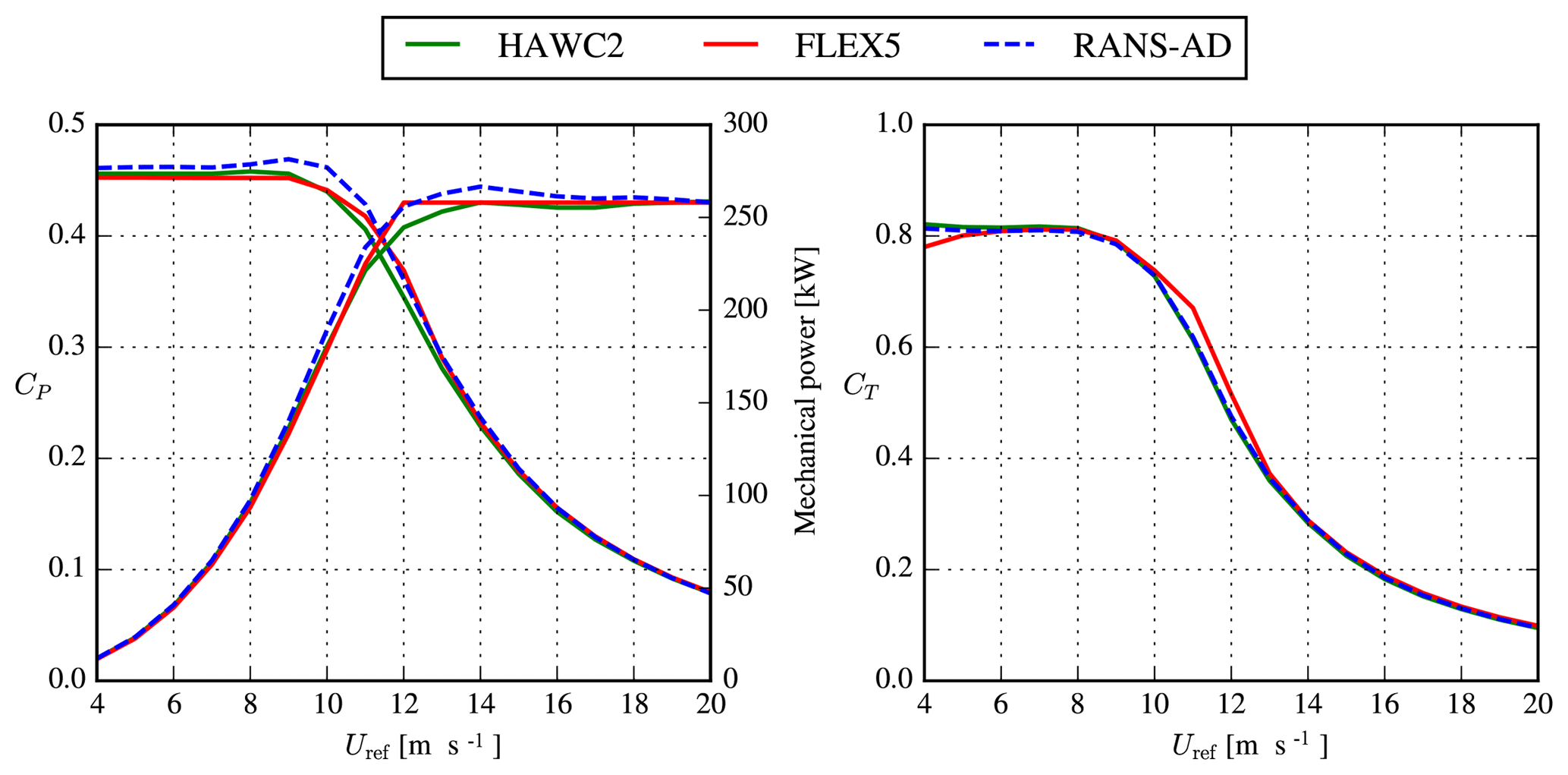
Figure 8 Comparison of simulated mechanical power and thrust of a single V29 rotor using HAWC2, FLEX5 and EllipSys3D RANS-AD.

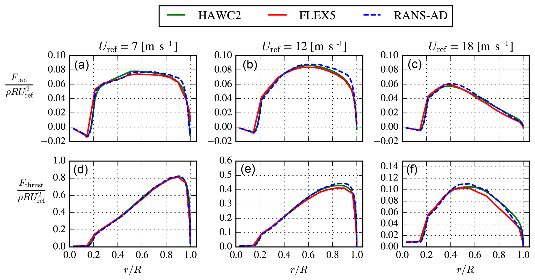
Figure 9 Comparison of simulated tangential (a–c) and thrust (d–f) force distribution of a single V29 rotor using HAWC2, FLEX5 and EllipSys3D RANS-AD.

4 Results and discussion

4.1 Comparison of V29 rotor models

A comparison of the V29 rotor models from EllipSys3D RANS-AD and FLEX5 (used by EllipSys3D LES-AL-FLEX5 and MIRAS-FLEX5) is made with a HAWC2 model of the V29 provided by Vestas Wind System A/S. The Fuga rotor model is not compared with the other models because the chosen thrust force distribution is uniform and the total thrust force is a model input. Here, the deflections are switched off in FLEX5 and HAWC2 in order to make a fair aerodynamic comparison with EllipSys3D RANS-AD that can only model stiff blades. The near-wake model of Pirrung et al. (2016, 2017) is used in HAWC2, and a uniform inflow is employed without inflow turbulence or the presence of a wall.

The mechanical power and thrust force as function of the undisturbed wind speed are plotted in Fig. 8 for the three models: EllipSys3D RANS-AD, FLEX5 and HAWC2. For wind speeds between 5 and 8 m s⁻¹, all three models predict a similar power and thrust coefficients that differ by approximately 2 %. The thrust coefficient of EllipSys3D RANS-AD and HAWC2 only differ by around 1 % for all wind speeds, whereas EllipSys3D RANS-AD overpredicts the power coefficient by about 1 % below 9 m s⁻¹ and by 2 %–6 % for higher wind speeds. The largest differences between FLEX5 and HAWC2 are observed around the shoulder of the power curve, which is presumably caused by differences in control strategies.

The normalized tangential and thrust force distributions for three different wind speeds (7, 12 and 18 m s⁻¹) are plotted in Fig. 9 for HAWC2, FLEX5 and EllipSys3D RANS-AD. For a wind speed of 7 m s⁻¹ (below the rated wind speed), all three models predict similar force distributions. For the higher wind speeds (12 and 18 m s⁻¹), there are differences between the three models, mainly observed outboard and towards the blade tip, which could be related to the different tip corrections that are employed in each model.

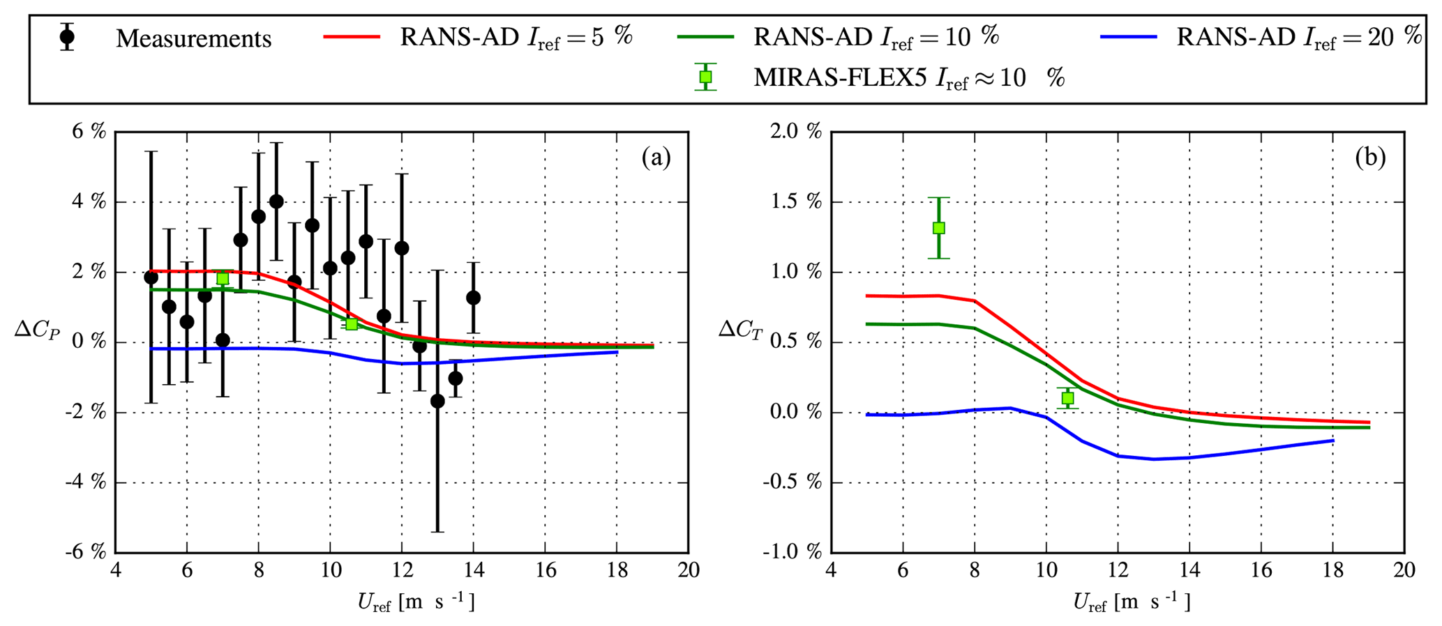
Figure 10 Relative difference between the 4R-V29 wind turbine with all rotors in operation and the 4R-V29 wind turbine with a single rotor in operation, in terms power and thrust as function of the free-stream velocity at a height of 44.27 m.

4.2 Performance of the 4R-V29 wind turbine

The measured and simulated relative difference in power (ΔC_P) and thrust force (ΔC_T) of the 4R-V29 wind turbine due to the rotor interaction are depicted in Fig. 10. ΔC_P and ΔC_T are calculated as follows:

$$\begin{array}{ll}\text{(4)}& {\displaystyle }& {\displaystyle }\mathrm{\Delta }{C}_P={\displaystyle \frac{\left(P_{R_{\mathrm{1}}}^{s_{\mathrm{2}}}+P_{R_{\mathrm{3}}}^{s_{\mathrm{2}}}\right)-\left(P_{R_{\mathrm{1}}}^{s_{\mathrm{1}}}+P_{R_{\mathrm{3}}}^{s_{\mathrm{3}}}\right)}{P_{R_{\mathrm{1}}}^{s_{\mathrm{1}}}+P_{R_{\mathrm{3}}}^{s_{\mathrm{3}}}}}{\displaystyle }& {\displaystyle }\mathrm{\Delta }{C}_T={\displaystyle \frac{\left(T_{R_{\mathrm{1}}}^{s_{\mathrm{2}}}+T_{R_{\mathrm{3}}}^{s_{\mathrm{2}}}\right)-\left(T_{R_{\mathrm{1}}}^{s_{\mathrm{1}}}+T_{R_{\mathrm{3}}}^{s_{\mathrm{3}}}\right)}{T_{R_{\mathrm{1}}}^{s_{\mathrm{1}}}+T_{R_{\mathrm{3}}}^{s_{\mathrm{3}}}}},\end{array}$$

where s₁, s₂ and s₃ correspond to the three stages of the test cycle as illustrated in Fig. 2, and P and T are the power and thrust force for a rotor R_i, respectively. The measurements in Fig. 10a show that the rotor interaction increases the power production of the 4R-V29 wind turbine for the wind speed bins below the rated wind speed between 7.5 and 11 m s⁻¹. The standard error of the mean ΔC_P is too large to make the same statement below 7.5 m s⁻¹. Above the rated wind speed, the effect of the rotor interaction on the mean power is smaller than below the rated wind speed, and high uncertainties of the mean power for 11.5 and 13 m s⁻¹ are observed. The weighted average of ΔC_P (using the number of observations per bin) for a wind speed between 5 and 11 m s⁻¹ is 1.8±0.2 %, which supports the observed bias towards a power gain below the rated wind speed. The rotor interaction of the 4R-V29 wind turbine increases the annual energy production by 1.5±0.2 % if we assume a Weibull distribution for the wind speed with shape and scale parameters of 2 and 7.5 m s⁻¹, respectively (corresponding to a mean wind speed of about 6.7 m s⁻¹), and we assume a zero power gain below 5 m s⁻¹ and above 11 m s⁻¹. The 0.2 % uncertainty represents the standard error of the mean and does not represent measurement uncertainties directly, which could be a lot higher than 0.2 %. However, the analysis is focused on the relative differences between the test cycles as illustrated in Fig. 4. In addition, we have removed uncertainties due to measurement biases as much as possible (e.g., induction correction), as discussed in Sect. 2.2.

The RANS-AD simulations in Fig. 10 are performed for three different turbulence intensities (5 %, 10 % and 20 %), and a larger power and thrust force below the rated wind speed is predicted when all four rotors are in operation for the two lowest turbulence intensities (5 % and 10 %). The largest gain in power (2 %) is found for the lowest turbulence intensity, where the shear is also the lowest. For a large turbulence intensity, the effect of the rotor interaction is almost zero below the rated wind speed. The loss in power above rated power is not interesting because it is possible to adapt the pitch angle such that the rated power is reached. Note that the V29 rotor starts to pitch out between 10 and 11 m s⁻¹. Figure 10b shows that ΔC_T from the RANS-AD simulations follow the trends of the ΔC_P. This indicates that the axial induction of the 4R-V29 wind turbine is increased due to the rotor interaction. The measured power gain including the standard error of the mean is of the same order as the RANS-AD simulations, except for the wind speed bins of 8.5, 11, 12 and 14 m s⁻¹, where the measured power gain is underpredicted by the simulations. The lower measured power gain for wind speeds below 7.5 m s⁻¹ compared with wind speeds between 7.5 and 9.5 m s⁻¹ could also be related to the fact that a high turbulence intensity is more common at low wind speeds, and the RANS-AD simulations show that the power gain decreases with increasing turbulence intensity.

Figure 11 The rotor individual relative difference between the 4R-V29 wind turbine with all rotors in operation and the 4R-V29 wind turbine with a single rotor in operation, in terms of power and thrust as function of the free-stream velocity at a height of 44.27 m.

Two results of MIRAS-FLEX5 for respective wind speeds of 7 and 10.6 m s⁻¹ using the Mann inflow turbulence of the far-wake case, which has a turbulence intensity of about 10 %, are also depicted in Fig. 10. Each result represents the mean of two consecutive 10 min averages, and the error bar represents the standard error of the mean. The power gain predicted by MIRAS-FLEX5 for respective wind speeds of 7 and 10.6 m s⁻¹ is 0.3 % higher and 0.1 % lower, respectively, compared with the results from RANS-AD (for a turbulence intensity of 10 %); however, the trend regarding wind speed is the same. The gain in the thrust coefficient from MIRAS-FLEX5 is 0.7 % higher and 0.1 % lower than RANS-AD for 7 and 10.6 m s⁻¹, respectively. The higher gains for 7 m s⁻¹ from MIRAS-FLEX5 are not caused by a difference in domain blockage when operating one or four rotors as the effects of domain blockage are avoided, as discussed in Sect. 3.3.

ΔC_P and ΔC_T for a bottom rotor (R₁) and a top rotor (R₃) calculated by the RANS-AD simulations for three different turbulence intensities are plotted in Fig. 11. The measurements in Fig. 11 also depict ΔC_P for one bottom (R₁) and one top rotor (R₃). The RANS-AD simulations indicate that the difference in ΔC_P and ΔC_T within a horizontal pair (R₁ compared to R₂ and R₃ compared to R₄) is negligible (results of R₂ and R₄ are not shown in Fig. 11 to improve readability), whereas the difference between a vertical pair is clearly visible. The bottom rotors produce more ΔC_P and ΔC_T than the top rotors, and the difference between the bottom and the top pair increases with turbulence intensity, which is probably due to associated increased shear. For the largest turbulence intensity (20 %) and shear (α=0.25), only the bottom rotors produces more power, which could be caused by the difference in thrust force between the top and bottom rotors. In other words, the high thrust force of the top rotors creates a blockage effect that pushes more wind downwards into the rotor plane of the bottom rotors. Two results of MIRAS-FLEX5, corresponding to respective wind speeds of 7 and 10.6 m s⁻¹ and a turbulence intensity of about 10 %, confirm that the bottom rotors produce more ΔC_P and ΔC_T than the top rotors. In addition, the difference between MIRAS-FLEX5 and RANS-AD is largest for the bottom rotor for 7 m s⁻¹ in terms of ΔC_T (1 %), where MIRAS-FLEX5 also shows the largest standard error of the mean because the lower rotor experiences a lower inflow wind speed and a higher turbulence level compared with the top rotor. The measurements also indicate that the bottom rotor is mainly responsible for the power gain, although the standard error of the mean of the bottom and top rotor overlap for most of the wind speed bins. In addition, one could argue that the sloping terrain, as illustrated in Fig. 5, may have influenced the difference between the top and the bottom pair, as sloping terrain can lead to a speedup close to the ground that enhances the wind resource for the lower rotor pair. The terrain effects could be included and studied in future work.

Figure 12 Near-wake case: contours of stream-wise velocity at three downstream distances.

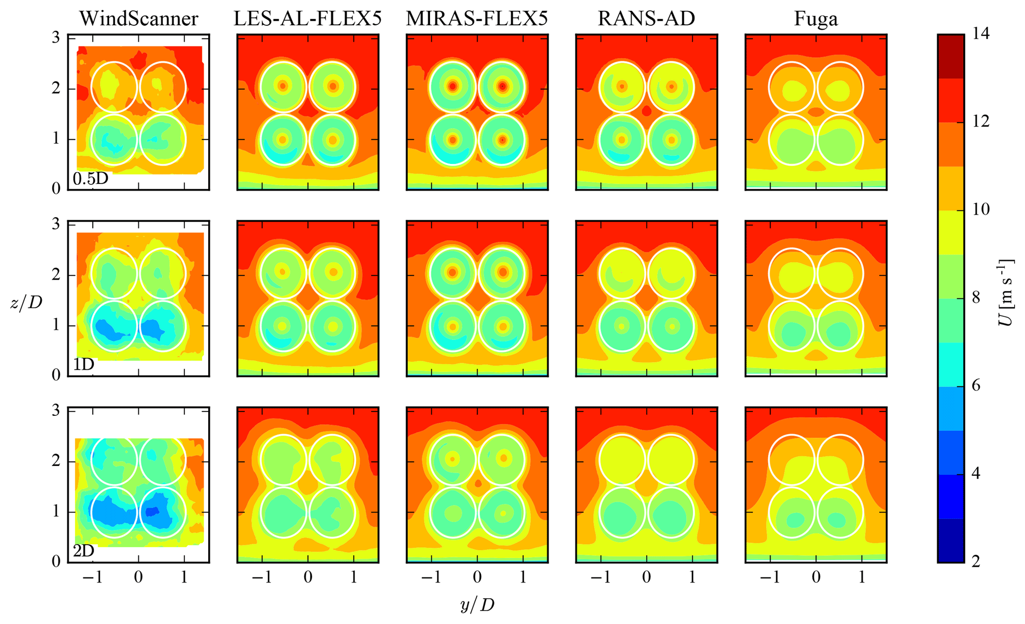
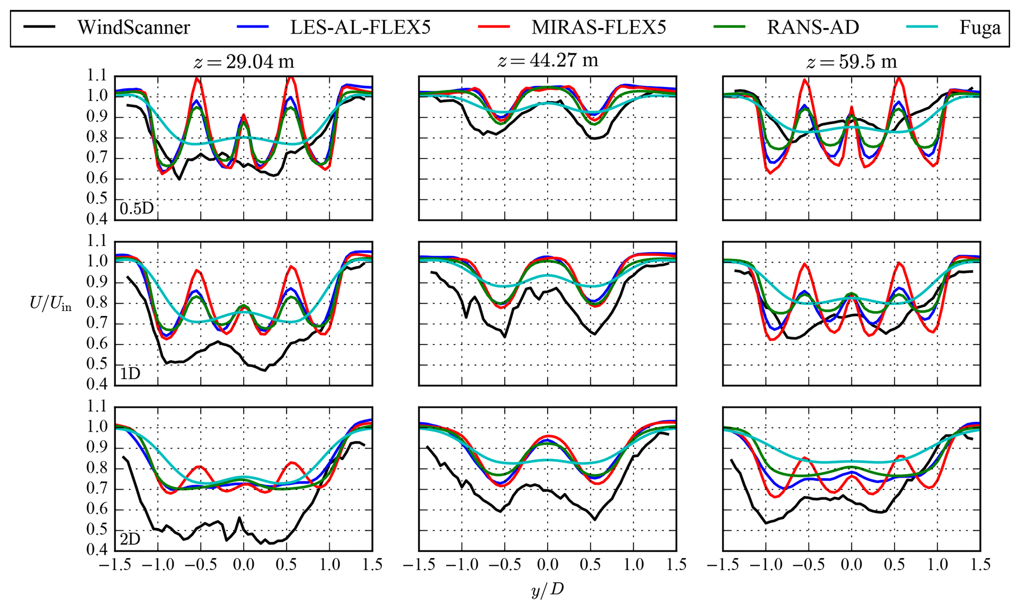
Figure 13 Near-wake case: profiles of stream-wise velocity at three heights and three downstream distances.

4.3 Wake deficit of the 4R-V29 wind turbine

Results of the near-wake test case are discussed in Sect. 4.3.1, whereas Sect. 4.3.2 presents results of the far-wake test case including the near-wake to far-wake development.

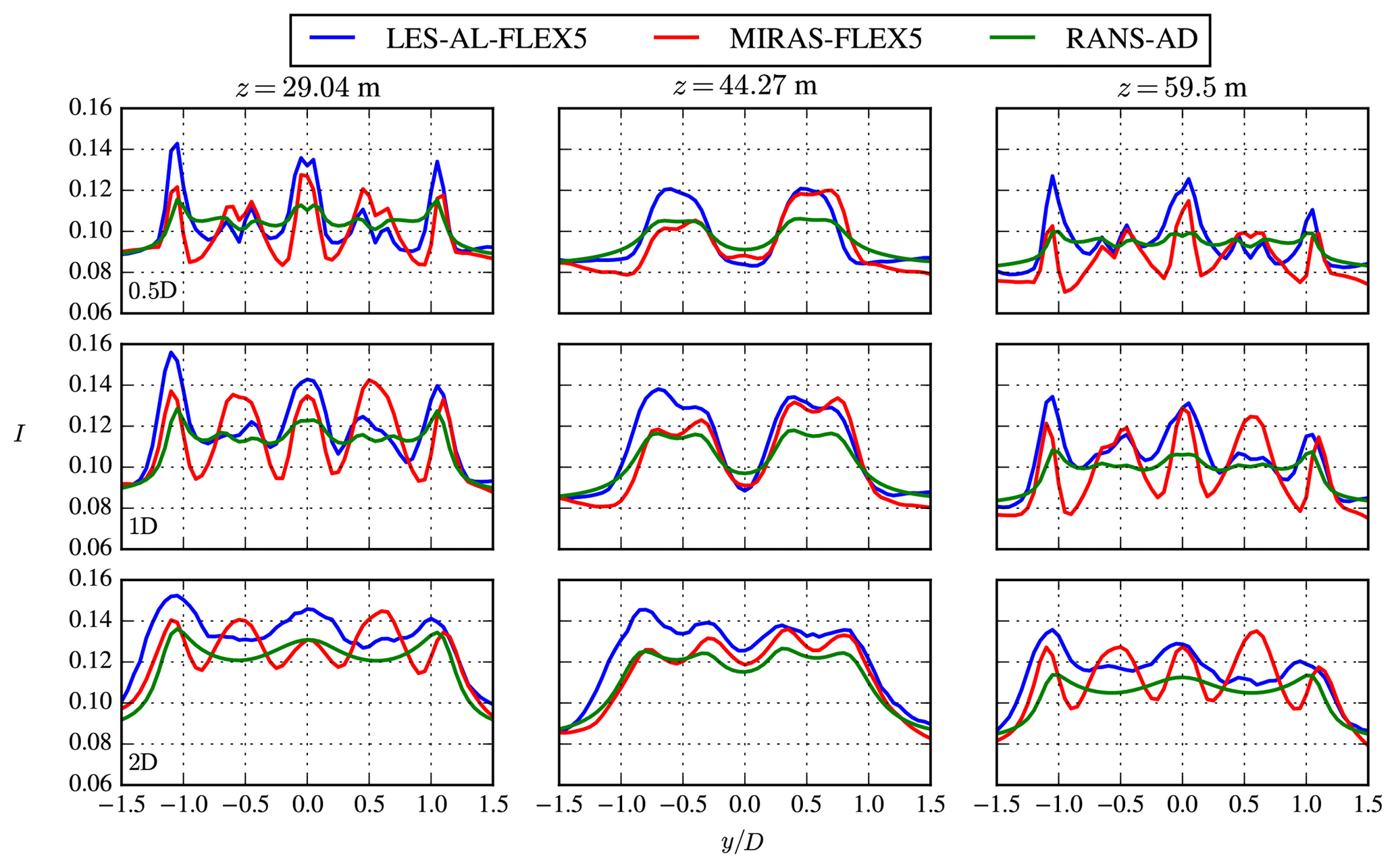
Figure 14 Near-wake case: profiles of turbulence intensity at three heights and three downstream distances.

4.3.1 Near-wake case

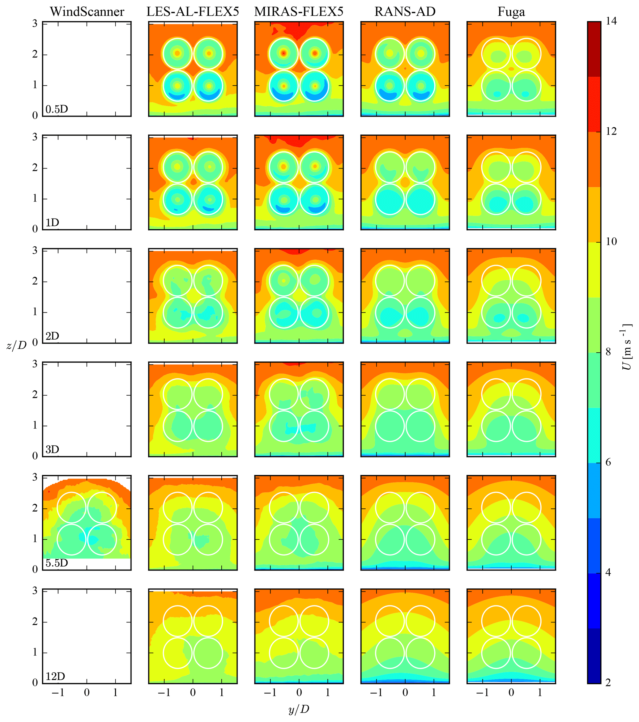
Contours of the stream-wise velocity at three downstream distances, measured by the short-range WindScanner and simulated by four models (LES-AL-FLEX5, MIRAS-FLEX5, RANS-AD and Fuga) are depicted in Fig. 12. The measurements and simulations show four distinct wakes, which are most visible at $x/D=\mathrm{0.5}$. At this distance, the measurements and Fuga show a stronger deficit at the bottom rotors compared with the top rotors, which is also visible in the RANS-AD results with smaller differences between the top and bottom rotors. The mixing in the surface layer linearly increases with height in RANS-AD and Fuga, which increases the mixing of the top rotors compared with the bottom rotors. In the higher fidelity models – LES-AL-FLEX5 and MIRAS-FLEX5 – the inflow turbulence is modeled by Mann turbulence that has a uniform turbulent mixing in the vertical direction. This could explain why LES-AL-FLEX5 and MIRAS-FLEX5 do not show a clear difference in wake deficit between the bottom and top rotors. Note that all models include a sheared inflow, which can also cause a difference in the wake deficit between the top and bottom rotors. At $x/D=\mathrm{2}$, the measurements show much lower velocities compared with all four models.

Profiles of the stream-wise velocity normalized by the inflow at three heights, corresponding to the bottom rotor hub height (29.04 m), the center reference height (44.27 m) and the top rotor hub height (59.5 m) are plotted in Fig. 13. Results of the WindScanner and the four models are shown, taken at three downstream distances. It is clear that measured velocity inside and outside of the wake, at the bottom rotor hub height and at the center height are lower than predicted by all four models. This suggests that the actual shear and reference wind speed at the 4R-V29 wind turbine could have been different to values measured at the reference met mast. Unfortunately, it is not possible to determine the free-stream conditions from the WindScanner data because of the limited horizontal extent of the scanned planes. In addition, the atmospheric conditions of the near-wake case measured at the reference met mast was near-neutral (see Table 1), which could have increased the measured wake deficit.

The measurements and all of models, except Fuga, show the buildup of a traditional double bell-shaped near-wake profile at the center height in the downstream direction, as depicted in Fig. 13. Fuga is based on a linearized RANS approach, which means that it is designed to describe the far wake properly; however, it cannot predict the nonlinear near wake accurately, especially for a high thrust coefficient, as shown by Ebenhoch et al. (2017). Nevertheless, the other models yield very similar results.

Profiles of the turbulence intensity I ($I=\sqrt{\mathrm{2}/\mathrm{3}k}/U_{\mathrm{ref}}$) are plotted in Fig. 14 using the same definition as in Fig. 13. Only the results of LES-AL-FLEX5, MIRAS-FLEX5 and RANS-AD are shown, as the WindScanner cannot measure I, and Fuga cannot model I in the wake because it uses a turbulence closure that is unaffected by the wake. Figure 14 shows that RANS-AD has smaller peaks in I to LES-AL-FLEX; this is due to the fact that an AD model simulates a ring root and tip vortex, whereas an AL model resolves a (smeared) root and tip vortex per blade.

Figure 15 Far-wake case: contours of stream-wise velocity at three downstream distances.

4.3.2 Far-wake case

The results of the far-wake case are plotted in Figs. 15, 16 and 17, which follow the same definition as in Figs. 12, 13 and 14, respectively. In addition, six downstream distances are depicted to show the full downstream development of the 4R-V29 wind turbine wake. Only measurements of the stream-wise velocity at $x/D=\mathrm{5.5}$ are available. The four individual wakes merge into a single structure between $x/D=\mathrm{2}$ and $x/D=\mathrm{3}$ as shown in Figs. 15 and 16. The middle column of Fig. 16 depicts how a bell-shaped near-wake structure forms at the center height up to and including $x/D=\mathrm{3}$, whereas the single wakes at the bottom and top hub heights cannot be distinguished from each other at this distance. Further downstream, at $x/D=\mathrm{5.5}$, the fifth row of plots in Fig. 15 shows that all models capture the measured single-wake structure at $x/D=\mathrm{5.5}$, although the wake of Fuga has moved downwards compared with the measurements and other models. The magnitude of the wake deficit at $x/D=\mathrm{5.5}$ is underpredicted by all models, as seen in Fig. 16, where the measured wake at the bottom hub height is also skewed. The measured wake skewness could be a terrain effect or a results of the 8.2^∘ yaw misalignment, as discussed in Sect. 2.3. In addition, the close proximity of the highway and surrounding trees, as discussed in Sect. 2.3, could have influenced the measurements of the far wake. Furthermore, we would like to point out that it is challenging to compare the models with a single 8 min averaged result from the WindScanner.

Figure 16 Far-wake case: profiles of stream-wise velocity at three heights and six downstream distances.

The inflow Mann turbulence that is used in LES-AL-FLEX5 and MIRAS-FLEX5 results in a turbulent kinetic energy profile that has a higher value near the ground and a lower value above the center height compared with the reference turbulent kinetic energy at the center height. The turbulent kinetic energy profile in the RANS-AD simulations is constant with height. Hence, the comparison of the RANS-AD simulations with the LES-AL-FLEX5 and MIRAS-FLEX5 simulations in terms of turbulence intensity (Fig. 17) at z=29.04 m and z=59.5 m is not entirely fair. At the center height (z=29.04 m), where the ambient turbulence intensity levels between the models are similar, the turbulence intensity in the far wake is higher in the RANS-AD simulations compared with LES-AL-FLEX5 (about 0.02 at $x/D=\mathrm{12}$, $y/D=\mathrm{0}$), which was also previously observed by van der Laan et al. (2015) for single AD simulations. The largest difference in turbulence intensity between the LES-AL-FLEX5 and MIRAS-FLEX5 simulations are found in the near wake for the lowest rotor pair (z=29.04 m).

The presented near- and far-wake cases show that the models follow the measured trends, but there are not enough measured data to validate the simulations. More wake measurements of the 4R-V29 wind turbine are required in order to perform a model validation.

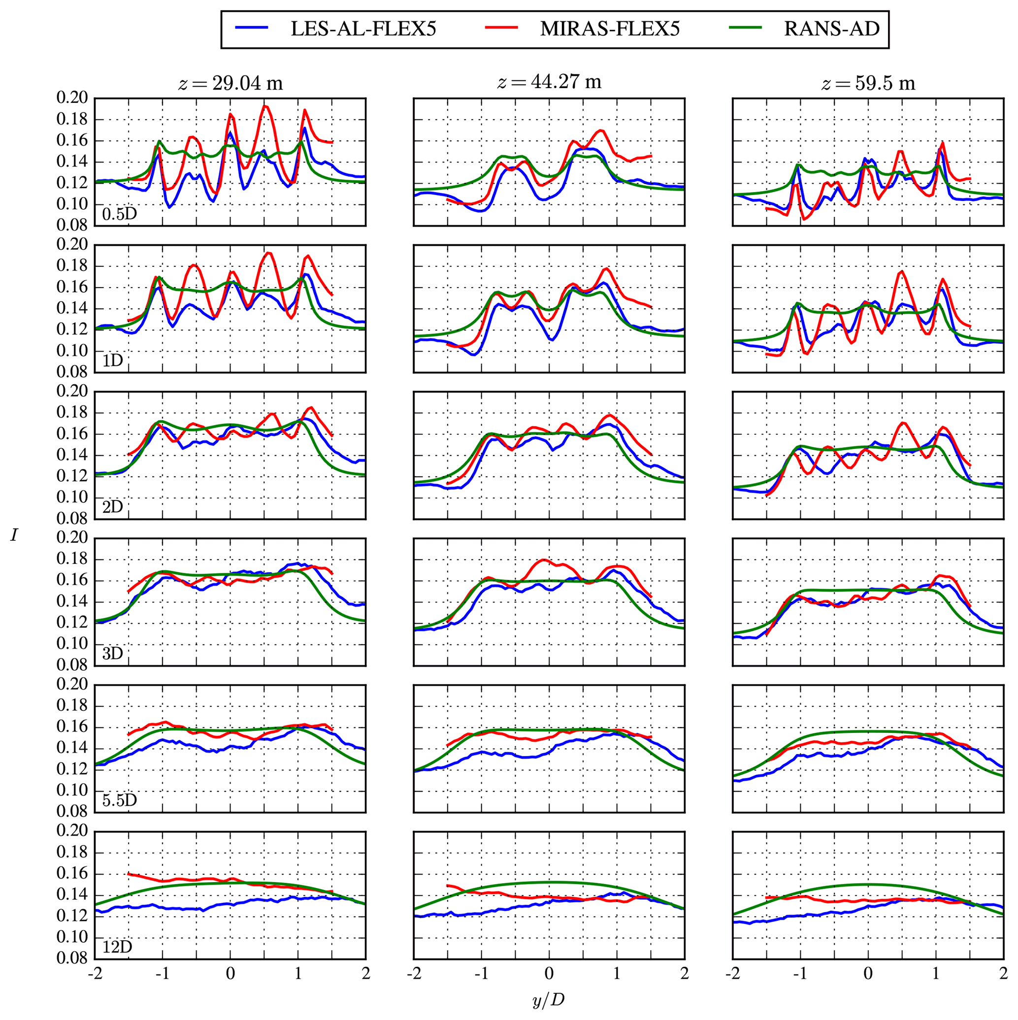
Figure 17 Far-wake case: profiles of turbulence intensity at three heights and six downstream distances.

Table 2 Definition of the simplified 4R-V29 multi-rotor wind turbine and an equivalent V58 single-rotor wind turbine for three ambient turbulence intensities.

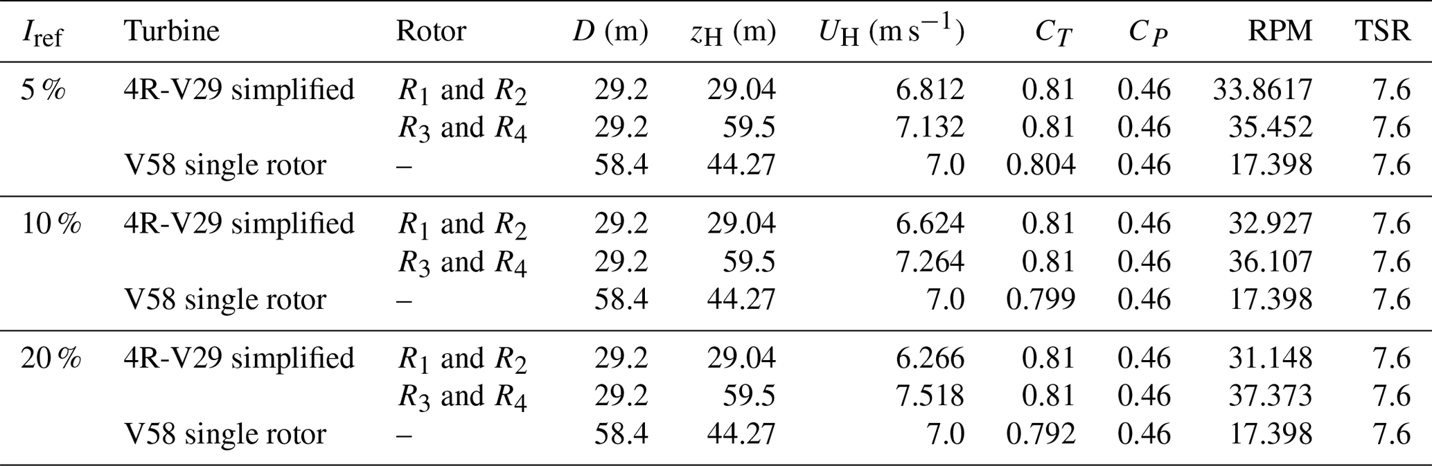
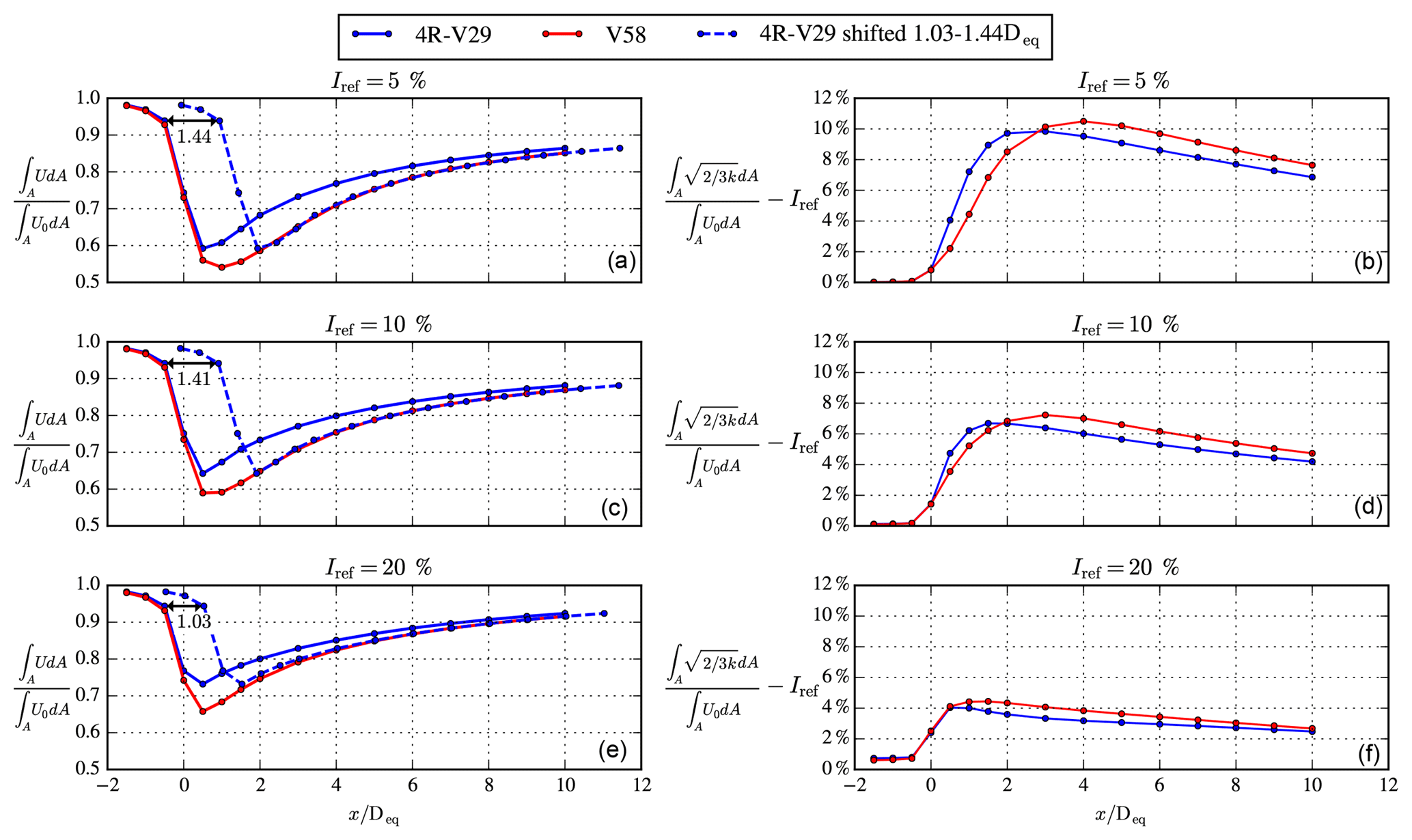
Figure 18 RANS predicted wake recovery of a simplified 4R-V29 multi-rotor wind turbine compared with an equivalent V58 single-rotor wind turbine for three difference turbulence intensities. (a, c, e) Integrated stream-wise velocity; (b, d, f) integrated added turbulence intensity. The dashed blue line is the integrated stream-wise velocity of the simplified 4R-V29 wind turbine shifted by 1.03–1.44 D.

4.4 Wake recovery of the 4R-V29 wind turbine

The wake recovery of a multi-rotor wind turbine is very important for placing several multi-rotors together in wind farms. Therefore, the aim here is to quantify the wake recovery of a multi-rotor wind turbine operating in an atmospheric surface layer with respect to an equivalent single-rotor wind turbine that has the same rotor area, force distributions, tip speed ratio (TSR) and total thrust force. In order to do so, a simplification of the 4R-V29 wind turbine is used so that a fair comparison with a equivalent single-rotor wind turbine can be made. The simplified 4R-V29 wind turbine has a zero toe-out angle, and the force distributions are defined by prescribed normalized blade force distributions (calculated by Réthoré et al., 2014, employing a detached eddy simulation of the NREL-5MW rotor for a wind speed of 8 m s⁻¹). The blade force distributions are scaled by the hub height velocity U_H, R, C_T, C_P and the rotational speed (RPM) as discussed by van der Laan et al. (2015). The resulting AD force distributions are uniform over the azimuth, and the effect of shear on the AD force distributions are neglected. The dimensions and scaling parameters of the simplified 4R-V29 wind turbine and an equivalent single-rotor wind turbine referred as V58, are summarized in Table 2. The inflow is an atmospheric surface layer, with U_ref=7 m s⁻¹ and three different I_ref at z_ref=44.27 m: 5 %, 10 % and 20 %. The hub height wind speed for the bottom and top rotor pairs is different for the simplified 4R-V29 wind turbine due to the shear. In order to model the same total thrust force for the V58 wind turbine, the thrust coefficient of the V58 is adjusted. The rotational speed is set to assure a TSR of 7.6 for all rotors.

Figure 18 depicts the wake recovery in terms of stream-wise velocity and added turbulence intensity of the simplified 4R-V29 multi-rotor wind turbine and the equivalent V58 single-rotor wind turbine as a function of the stream-wise distance x normalized by the single-rotor diameter (D_eq=58.4 m) for three turbulence intensities (5 %, 10 % and 20 %). The wake recovery is calculated as rotor-integrated values normalized by the same integral without an AD. Note that four integrals are calculated for the multi-rotor and summed up for each downstream distance. Figure 18a, c and e show that the wake recovery distance in terms of stream-wise velocity of a simplified 4R-V29 multi-rotor wind turbine is about 1.03–1.44 D_eq shorter than the wake recovery distance of a V58 single-rotor wind turbine, which is a remarkable difference. The largest difference is found for the lowest ambient turbulence intensities (5 %). This suggests that the horizontal area of a wind farm consisting of 4R-V29 wind turbines positioned in a regular rectangular layout can be reduced compared with a wind farm consisting of V58 wind turbines. The area could be reduced by $\mathrm{1}-(\mathrm{1}-\mathrm{1.44}/s{)}^{\mathrm{2}}$ and $\mathrm{1}-(\mathrm{1}-\mathrm{1.03}/s{)}^{\mathrm{2}}$ (for I_ref=5 % and I_ref=20 %, respectively), with s as the horizontal and vertical inter-turbine spacing in D_eq. For example, for s=8 D_eq the RANS predicted reduction in wind farm area would be 24 %–32 %; this significant reduction in the area required could also reduce cost and potentially increase the power production by increasing the number of installed turbines in a given area. This result is a rough extrapolation that should be verified by wind farm simulations of multi-rotor wind turbines.

Figure 18b, d and fshow that the added wake turbulence is larger for the multi-rotor wind turbine in the near wake for I_ref=5 % and I_ref=10 % for $x/D_{\mathrm{eq}}<\mathrm{3}$ and $x/D_{\mathrm{eq}}<\mathrm{2}$, respectively, but is smaller in the far wake with respect to the added wake turbulence of single-rotor wind turbine. It is not possible to shift the added wake turbulence of the multi-rotor wind turbine downstream to match the added wake turbulence of the single-rotor wind turbine in the same manner as the wake recovery. The lower wake turbulence in the far wake has the potential to reduce blade fatigue loads that are caused by wake turbulence.

The increased wake recovery of a multi-rotor wind turbine could be related to the fact that the total thrust force is more distributed compared with a single-rotor wind turbine. Ghaisas et al. (2018) also obtained a faster wake recovery for a multi-rotor wind turbine, and argued that it is caused by a larger entrainment because the ratio of the rotor perimeter and the rotor swept area is twice as high for the multi-rotor wind turbine with four rotors.

5 Conclusions

Numerical simulations and field measurements of the Vestas multi-rotor wind turbine (4R-V29) have been performed. The simulations show an increased thrust force and axial induction of the 4R-V29 wind turbine compared with a single rotor. In addition, the simulations calculate a 0 %–2 % enhancement of the power performance of the 4R-V29 multi-rotor wind turbine below the rated wind speed due to the interaction of the rotors. The largest gain in power is obtained for a low turbulence intensity that is associated with a low shear. The relative power gain is largest for the bottom rotor pair. Power curve measurements of the 4R-V29 wind turbine also show that rotor interaction increases the power performance below the rated wind speed by 1.8 %, which can result in a 1.5 % increase in the annual energy production.

Two flow cases based on short-range WindScanner wake measurements of the 4R-V29 wind turbine are used to compare the multi-rotor wake deficit simulated by four numerical models. In the near wake, four distinct wake deficits are visible that merge into a single structure at a downstream distance of 2–3 D. More wake measurements are required to validate the numerical models.

The wake recovery of a simplified 4R-V29 wind turbine is quantified by comparison with the wake recovery of an equivalent single-rotor V58 wind turbine. RANS simulations show that the wake recovery distance in terms of the stream-wise velocity of the simplified 4R-V29 wind turbine is 1.03–1.44 D_eq shorter than a the wake recovery distance of the equivalent single-rotor wind turbine with a rotor diameter D_eq. In addition, it is found that the added wake turbulence of the simplified 4R-V29 wind turbine is smaller than the equivalent single-rotor V58 wind turbine in the far wake. The fast wake recovery of a multi-rotor wind turbine could potentially lead to closer spaced wind turbines in multi-rotor wind farms and needs to be further investigated.

Appendix A: Induction correction for the measured reference wind speed for the power curve measurements of the 4R-V29 wind turbine

The measured effect of rotor interaction on the power production is quantified using the test cycle in Fig. 2, where the combined power curves of two single-rotor operation stages (stages 1 and 3) are compared with the power curve of a stage where all four rotors are in operation (Stage 2). The reference wind speed in these power curve measurements is taken at 5 D (146 m) upstream, as discussed in Sect. 2.2. As the induction zone in stages 1 and 3 is smaller than in Stage 2, a lower reference wind speed is measured when all four rotors are in operation. Hence, the power curve of Stage 2 will be shifted towards the left, and an artificial bias towards a power gain due to the rotor interaction would be measured. To avoid this, the reference wind speed is corrected by a factor f_cor when all four rotors are in operation (Stage 2):

$$\begin{array}{}\text{(A1)}& {\displaystyle }{f}_{\mathrm{cor}}={\displaystyle \frac{\frac{\mathrm{1}}{\mathrm{2}}\left(U_{\mathrm{ref}}^{\mathrm{Stage},\mathrm{1}}+U_{\mathrm{ref}}^{\mathrm{Stage},\mathrm{3}}\right)}{U_{\mathrm{ref}}^{\mathrm{Stage},\mathrm{2}}}}\end{array}$$

for each undisturbed wind speed with an interval of 1 m s⁻¹. The induction correction factor can only be calculated if the undisturbed wind speed is known. Therefore, the RANS simulations in Sect. 3.2.2 are used to calculate f_cor, and the results are shown in Fig. A1 for a reference turbulence intensity of 10 %. f_cor follows the thrust coefficient curve, and below the rated wind speed, where the thrust coefficient is the highest, the measured reference wind speed for Stage 2 is 0.7 % lower than the reference wind speed in stages 1 and 3.

f_cor is also calculated using a simple induction model from Troldborg and Meyer Forsting (2017), which has been developed to model the induction of a single rotor in a uniform inflow. The simple induction model is only a function of the thrust coefficient, rotor radius and spatial coordinates. The thrust coefficient of the RANS simulations is used as input. The induction zone for Stage 2 is calculated by superposition of the induction of the four individual rotors. Figure A1 shows that the induction of the 4R-V29 wind turbine at $x=-\mathrm{5}$ D is underestimated by the simple induction model compared with the RANS simulations and should not be used to correct of the reference wind speed in Stage 2. We chose to use the RANS results to correct the reference wind speed, as Meyer Forsting et al. (2017) have shown that RANS-AD simulations compare well with lidar measurements of the induction zone when measurement uncertainty is included in the validation method.

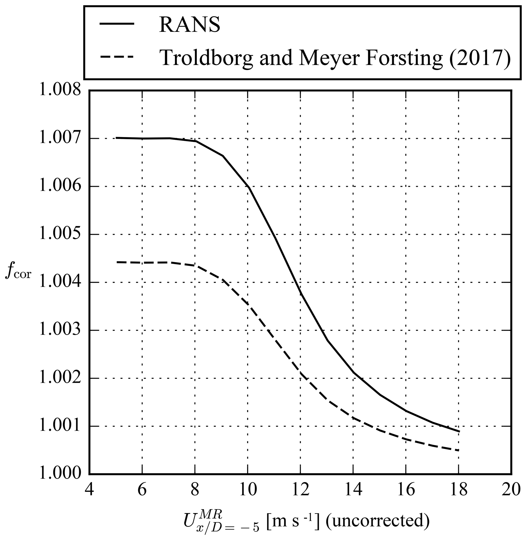
Figure A1 Induction correction factor for the measured reference wind speed of the 4R-V29 wind turbine.

The influence of the ambient turbulence intensity at a height of 44.27 m on f_cor in the RANS simulations is also investigated for three different turbulence intensities (5 %, 10 % and 20 %). The results are same for a turbulence intensity of 5 % and 10 %, whereas the f_cor is slightly higher for a turbulence intensity of 20 % (f_cor=1.0073 below the rated wind speed). As the power curve measurements are filtered for a wind direction from the fjord, we expect that the ambient turbulence intensity is lower than 20 % and that a f_cor based on a turbulence intensity of 10 % is justified.

Appendix B: Nomenclature

D	Rotor diameter of each single rotor of the 4R-V29
	wind turbine.
Deq	Rotor diameter of an equivalent single rotor wind
	turbine (Deq=2 D).