Uncertainty identification of blade-mounted lidar-based inflow wind speed measurements for robust feedback–feedforward control synthesis

The current trend toward larger wind turbine rotors leads to high periodic loads across the components due to the non-uniformity of inflow across the rotor. To address this, we introduce a blade-mounted lidar on each blade to provide a preview of inflow wind speed that can be used as a feedforward control input for the mitigation of such periodic blade loads. We present a method to easily determine blade-mounted lidar parameters, such as focus distance, telescope position, and orientation on the blade. However, such a method is accompanied by uncertainties in the inflow wind speed measurement, which may also be due to the induction zone, wind evolution, “cyclops dilemma”, unidentified misalignment in the telescope orientation, and the blade segment orientation sensor. Identification of these uncertainties allows their inclusion in the feedback–feedforward controller development for load mitigation. We perform large-eddy simulations, in which we simulate the blade-mounted lidar including the dynamic behaviour and the induction zone of one reference wind turbine for one above-rated inflow wind speed. Our calculation approach provides a good trade-off between a fast and simple determination of the telescope parameters and an accurate inflow wind speed measurement. We identify and model the uncertainties, which can then be directly included in the feedback–feedforward controller design and analysis. The rotor induction effect increases the preview time, which needs to be considered in the controller development and implementation.

1 Introduction

The ongoing trend of steadily growing rotor diameters of wind turbines results in dynamic loads across the rotor swept area which are becoming more uneven. Due to the so-called rotational sampling or eddy slicing effect, the blade samples the inhomogeneous wind field with frequencies determined by the rotor speed. Hence, the dynamic blade loads are concentrated at the multiples of the rotational frequency, i.e. 1P, 2P, 3P, …, nP (Bossanyi, 2003; van Engelen, 2006).

The scope of this paper is particularly geared to the relevance of three aspects of recent developments in controls to mitigate such loading. First, the control surfaces on the rotor are becoming more localized and consequently in addition to individual (blade) pitch control, local active or passive blade load mitigation concepts (e.g. trailing edge flaps) have been researched for several years. Second, in addition to the proven feedback control based on rotor speed and individual blade root bending moment measurements, feedforward control using either observer techniques or lidar-assisted preview information of the inflow has been investigated for collective and individual pitch as well as trailing edge flap control. Third, there are methods that can be applied in the feedback–feedforward controller design to guarantee robust stability and performance in the presence of inherent uncertainties in the lidar measurement.

The traditional collective pitch control (CPC) is responsible for keeping the rotor speed constant near and at above-rated wind speed conditions. Bossanyi (2003) extended the CPC with individual pitch control (IPC) to mitigate the 1P dynamic blade load. He demonstrated the effectiveness of the IPC in reducing the dynamic blade loads. Later, the function of the IPC was extended to address the mitigation of higher-harmonic dynamic blade loads (Bossanyi, 2005; van Engelen, 2006), leading to load relief across the wind turbine components, i.e. blade root bending moments, hub yaw and tilt moments, yaw bearings, etc. Such a control design leads to the increased use of the blade pitch system. With growing blade length, the blade mass rises with a power of 2 to 3, and thus increased pitch activity becomes even more undesirable and as such results in wear and tear of the pitch actuators and bearings and, equivalently, higher maintenance costs. One solution involves the use of small localized control surfaces to locally influence the thrust force. Pechlivanoglou (2013) conducted experimental and numerical studies to determine the most promising set-up of passive and active local flow control solutions for wind turbine blades, and he concluded that a controllable flexible trailing edge flap close to the blade tip has the most potential to mitigate the dynamic blade loads. The individual trailing edge flap control (TEFC) has been shown to be an effective means of reducing dynamic blade loads in numerical studies (Bergami and Poulsen, 2015; He et al., 2018; Ungurán and Kühn, 2016; Zhang et al., 2018), wind tunnel tests (Barlas et al., 2013; Marten et al., 2018; van Wingerden et al., 2011), and field tests (Berg et al., 2014; Castaignet et al., 2014). Castaignet et al. (2014) performed a full-scale test on a Vestas V27 wind turbine, reporting a load reduction of 14 % at the flap-wise blade root bending moment, providing proof of the control concept and the capabilities of the trailing edge flap for dynamic blade load mitigation.

Recently, feedforward control has been identified as a promising concept for wind turbine control, as feedback controllers mainly rely on indirect measurement of the disturbance, e.g. through measurement of rotor speed deviation from rated rotor speed or measurement of the blade root bending moment. Feedback controllers are only able to react on the disturbance after its influence on the wind turbine has been measured, which leads to a delayed control action. Several authors propose lidar-assisted wind turbine controllers so that control actions can be determined before the disturbance influences the turbine. When properly tuned, this so-called feedforward control strategy can mitigate fatigue loading from external disturbances. The lidar-assisted collective pitch controller proposed by Schlipf et al. (2013) accomplished a better rotor speed tracking with reduced pitch activity with respect to the feedback collective pitch controller. They also demonstrated reductions of damage-equivalent loads for the out-of-plane blade root bending moment, low-speed shaft torque, and tower bottom fore–aft bending moment through the use of lidar measurements in determining the feedforward collective pitch control input. Bossanyi et al. (2014); Kapp (2017) investigated the use of lidar for feedback–feedforward collective and individual pitch control and concluded its suitability for wind turbine control applications. Their purpose for the IPC was to mitigate the 1P loads at the flapwise blade root bending moment. They observed that a lidar-assisted feedback–feedforward IPC achieves marginal damage-equivalent load reduction with respect to feedback-only IPC. Ungurán et al. (2019) achieved additional load reduction across various wind turbine components with a combined feedback–feedforward IPC when compared to feedback-only IPC. They highlighted that to further reduce the blade root bending moment and avoid undesirable load increases on other wind turbine components, special care should be taken as the feedback is combined with feedforward IPC during controller development, in terms of, for instance, avoiding the same bandwidth for the feedback and feedforward IPC. This results in an elevated peak in the sensitivity function around the crossover frequency. Furthermore, Bossanyi et al. (2014), Kapp (2017), and Ungurán et al. (2019) studied different inflow wind conditions and wind turbine characteristics; they also used different lidar systems for feedforward control purposes that influenced the results.

For obvious reasons, it is necessary to consider the uncertainties in the lidar measurements to achieve robust stability and performance of the feedback–feedforward controller. Furthermore, the source of such uncertainties must be identified and modelled, which can then be incorporated into the design and analysis of the controller, to ensure performance even for uncertain lidar measurements. Several authors have already addressed this problem, e.g. Bossanyi (2013), Laks et al. (2013), and Simley et al. (2014a, b) with their numerical investigations. Simley et al. (2016) performed field tests to assess the influence of the “cyclops dilemma”, spatial averaging error, induction zone, and wind evolution on a hub-mounted lidar measurement. Simley et al. (2014a) used a hub-mounted continuous-wave (CW) lidar to investigate the effect of the cyclops dilemma and concluded that a compromise in the preview distance existed. Spatial averaging increases with increasing distance from the rotor plane, leading to correlation attenuation between the rotor-effective wind speed and the lidar-estimated inflow wind speed, with increasing frequency. As measurements are taken closer to the rotor plane, the contribution of the lateral and vertical wind components to the line-of-sight lidar measurements also increases. Thus, it is not possible to accurately reconstruct the longitudinal wind component from a single hub-mounted lidar system, which results in over- or underestimation of the rotor effective wind speed. Laks et al. (2013) investigated how wind evolution affects controller performance; they used a single-point measurement, without spatial averaging, in front of the wind turbine blade as a feedforward IPC input. Using the feedback–feedforward IPC, they acquired the highest load reduction at the blade root bending moment at a preview time of only 0.2 s. The further the measurement was taken from the rotor plane, the more the wind evolved at high frequencies (i.e. the so-called “wind evolution”), leading to overactuation by the feedforward IPC. It should be noted that the required preview time depends on many factors, e.g. wind turbine size, 1P frequency, inflow wind speed, and induced phase shift by the feedforward controller and blade pitch actuators.

The blade-mounted lidar system is a novel technique that enables us to sample the wind component parallel to the rotor shaft axis around the swept area (Bossanyi, 2013) and has been demonstrated to be technologically viable (Mikkelsen et al., 2012). Such a feature of the system enables addressing the mitigation of higher-harmonic dynamic blade loads through feedback–feedforward individual pitch and trailing edge flap controllers (Ungurán et al., 2018, 2019), while simultaneously posing challenges with the presence of the induction zone. The closer the lidar measurement is taken to the rotor plane, the higher the deficit between the measured inflow and free flow wind speeds. Additionally, this deficit depends on where the lidar is mounted along the blade radius, which shows the importance of analysing how the blade-mounted lidar measurement is affected by wind evolution, the induction zone, and the assumptions made during the inflow wind speed reconstruction.

Therefore, in this study, our objective is to identify the nominal measurement transfer functions and model the uncertainties of the blade-mounted lidar measurement as a frequency-dependent uncertain weight for inclusion in the feedback–feedforward individual pitch and trailing edge flap control development and to analyse the impact of the induction zone effect on the preview time.

The rest of the paper is organized as follows. Sect. 2 provides a description of the framework and methods we use for identifying the uncertainties and preview time of the blade-mounted lidar measurement, after an introduction of the blade-mounted lidar-based simulation set-up in Sect. 2.1. In Sect. 2.2 we describe the method we use to estimate the inflow wind speed. The method we employed for determining the blade effective wind speed to assess the efficiency of the blade-mounted lidar-based inflow wind speed measurement is discussed in Sect. 2.3. Section 2.4 describes the general control implementation and presents the multiblade coordinate transformation and its importance in the controller design, while Sect. 2.5 details how the lidar-based measurement uncertainty is considered in control development and analysis. Section 2.6 proposes a method to identify the uncertainties of the blade-mounted lidar measurement as a frequency-dependent uncertainty weight, Sect. 2.7 presents the method we apply for estimating the preview time, and Sect. 2.8 introduces a cost function which we use to evaluate the initially selected lidar and telescope parameters. The results of a reference case are presented in Sect. 3, where in Sect. 3.1 we analyse the effect of the multiblade coordinate transformation on the measurement. The simulation set-up is established in Sect. 3.2, and we systematically analyse the uncertainties of various telescope and control parameters in Sect. 3.3. The results are discussed in Sect. 4 prior to the conclusions in Sect. 5.

2 Methodology

2.1 Blade-mounted lidar

A telescope is mounted on each blade and is connected to a hub-based continuous-wave lidar with fibre optical cables. The lidar samples the inflow wind speed in front of the rotor plane at a rate of 5 Hz, and we intend to use the lidar measurements for control purposes. The lidar measurements are integrated into the system model according to Fig. 1, and we use a combination of large-eddy simulations and an aeroelastic simulation code to simulate and evaluate the lidar-based inflow measurements. Thus, lidar measurements are simulated in a realistic environment, where the effect of the induction zone and wind evolution, as well as the dynamic behaviour of the wind turbine, are taken into account. Moreover, the lidar simulator considers volumetric measurement, dynamics of the blade and tower, i.e. displacement, rotation, and linear velocity in 3-D space, and blade-rotation-induced velocity. Nevertheless, the rotational effect of the blade is not accounted for during the accumulation of a single measurement.

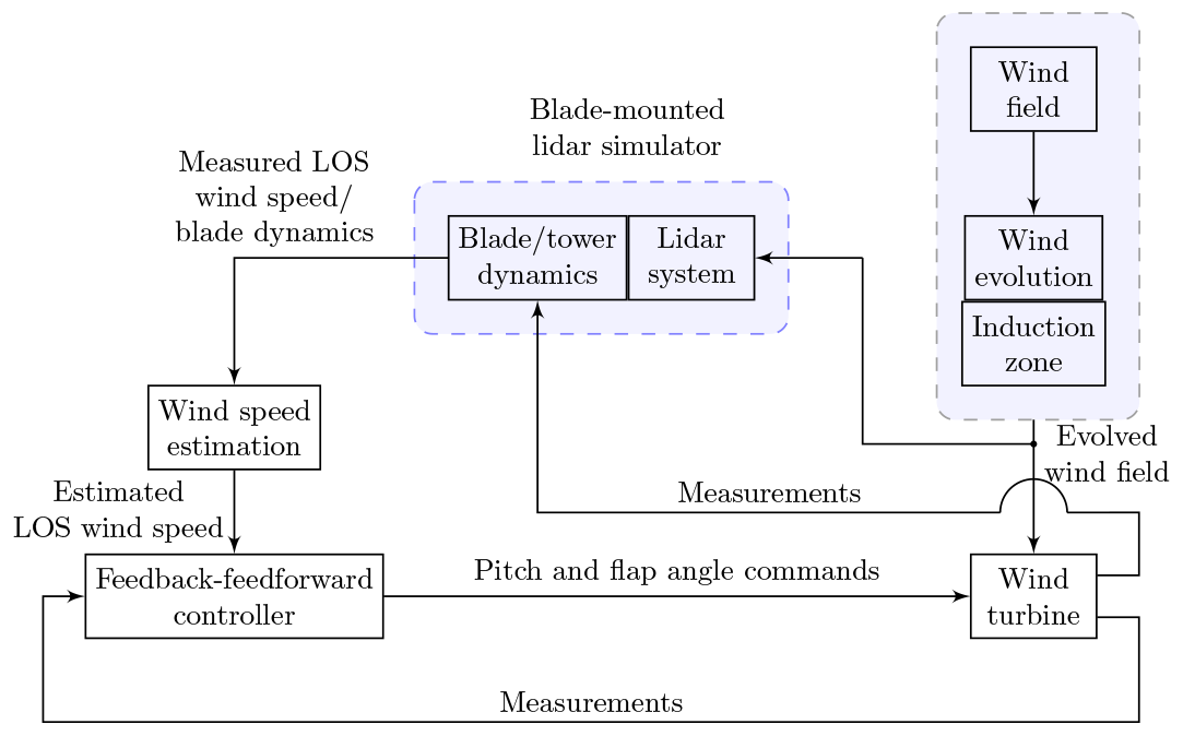
Figure 1 Block diagram of the blade-mounted lidar-based simulation set-up. LOS corresponds to line of sight.

Figure 2 Configuration of the lidar measurement system, with a telescope mounted on each blade and connected to a continuous-wave lidar in the hub via fibre optics. The line-of-sight wind speed is computed on the basis of a weighting function (W(F, ξ)), which is dependent on the focus distance (F) and the range along the beam (ξ).

Figure 2 illustrates the coordinate systems and the telescope orientation. Here, the line-of-sight (LOS) wind speed measurement from blade i (u_los,i) is defined as

$$\begin{array}{}\text{(1)}& u_{\mathrm{los},i}={\displaystyle \frac{\underset{{\mathit{\xi }}_{\min }}{\overset{{\mathit{\xi }}_{\max }}{\int }}W(F,\mathit{\xi })V_i\left(\mathit{\xi }\right)\mathrm{d}\mathit{\xi }}{\underset{{\mathit{\xi }}_{\min }}{\overset{{\mathit{\xi }}_{\max }}{\int }}W(F,\mathit{\xi })\mathrm{d}\mathit{\xi }}},\end{array}$$

where V_i(ξ) is defined in Eq. (3) and W(F, ξ) is the lidar's weighting function, defined according to Simley et al. (2014a) as

$$\begin{array}{}\text{(2)}& W(F,\mathit{\xi })={\displaystyle \frac{\mathrm{1}}{{\mathit{\xi }}^{\mathrm{2}}+{\left(\mathrm{1}-\frac{\mathit{\xi }}{F}\right)}^{\mathrm{2}}{R}_{\mathrm{R}}^{\mathrm{2}}}},\end{array}$$

where R_R is the Rayleigh range, set at 1573 m herein, as proposed by Simley et al. (2014a); F is the focus distance and ξ is the range along the beam. The limits ξ_min and ξ_max, introduced in Eq. (1), refer to the minimum and maximum range, respectively, along the beam. For a practical implementation of the lidar simulator, these values are chosen such that $\frac{W(F,\mathit{\xi })}{W(F,F)}$ equals 0.02 at these limits. During discretization of Eq. (1), the spatial resolution is set empirically at Δξ=0.1 m. A single-point measurement is given by

$$\begin{array}{}\text{(3)}& {\mathbf{V}}_i\left(\mathit{\xi }\right)={\left(\left[\begin{array}{c}{u}_{\mathrm{h},i}\left(\mathit{\xi }\right)\\ v_{\mathrm{h},i}\left(\mathit{\xi }\right)\\ w_{\mathrm{h},i}\left(\mathit{\xi }\right)\end{array}\right]-\left[\begin{array}{c}{\dot{x}}_{\mathrm{t},\mathrm{h},i}\\ {\dot{y}}_{\mathrm{t},\mathrm{h},i}\\ {\dot{z}}_{\mathrm{t},\mathrm{h},i}\end{array}\right]\right)}^T\left[\begin{array}{c}{\mathrm{\ell }}_{x,\mathrm{h},i}\\ {\mathrm{\ell }}_{y,\mathrm{h},i}\\ {\mathrm{\ell }}_{z,\mathrm{h},i}\end{array}\right],\end{array}$$

where $[u_{\mathrm{h},i}{v}_{\mathrm{h},i}{w}_{\mathrm{h},i}{]}^T$ is the wind speed vector along the laser beam expressed in the rotating hub coordinate system; $[{\dot{x}}_{\mathrm{t},\mathrm{h},i}{\dot{y}}_{\mathrm{t},\mathrm{h},i}{\dot{z}}_{\mathrm{t},\mathrm{h},i}{]}^T$ is the linear velocity vector of the blade segment where the telescope is mounted, expressed in the rotating hub frame of reference; and $[{\mathrm{\ell }}_{x,\mathrm{h},i}{\mathrm{\ell }}_{y,\mathrm{h},i}{\mathrm{\ell }}_{z,\mathrm{h},i}{]}^T$ is the unit vector of the laser beam in the rotating hub coordinate system. The aeroelastic simulation tool is capable of providing full kinematics information, i.e. positions, orientations, and linear and angular velocities, of any blade segment in the hub coordinate system.

2.2 Wind speed estimation

During the inflow wind speed estimation, the velocity, displacement, and rotation of the blade segment are assumed to be known; therefore, the wind speed component parallel to the rotor shaft axis can be reconstructed as indicated in Eq. (4). Without loss of generality, in the wind speed estimation, the weighting function of W(F,ξ) from Eq. (1) is neglected, and two assumptions are made: (1) the v_h,i and w_h,i components are zero, and (2) the mean wind velocity is parallel to the rotor axis; i.e. no tilt and no yaw misalignments are considered. Consequently, an estimate of the wind speed parallel to the rotor shaft axis ($u_{\mathrm{h},\mathrm{est},i}$) is

$$\begin{array}{}\text{(4)}& u_{\mathrm{h},\mathrm{est},i}\approx {\displaystyle \frac{u_{\mathrm{los},i}+{\dot{y}}_{\mathrm{t},\mathrm{h},i}{\mathrm{\ell }}_{y,\mathrm{h},i}+{\dot{z}}_{\mathrm{t},\mathrm{h},i}{\mathrm{\ell }}_{z,\mathrm{h},i}}{{\mathrm{\ell }}_{x,\mathrm{h},i}}}+{\dot{x}}_{\mathrm{t},\mathrm{h},i}.\end{array}$$

Nevertheless, such assumptions introduce errors into the lidar measurement that are presumed to exist in the identified uncertainty weight and, thus, are consequently considered during the controller development.

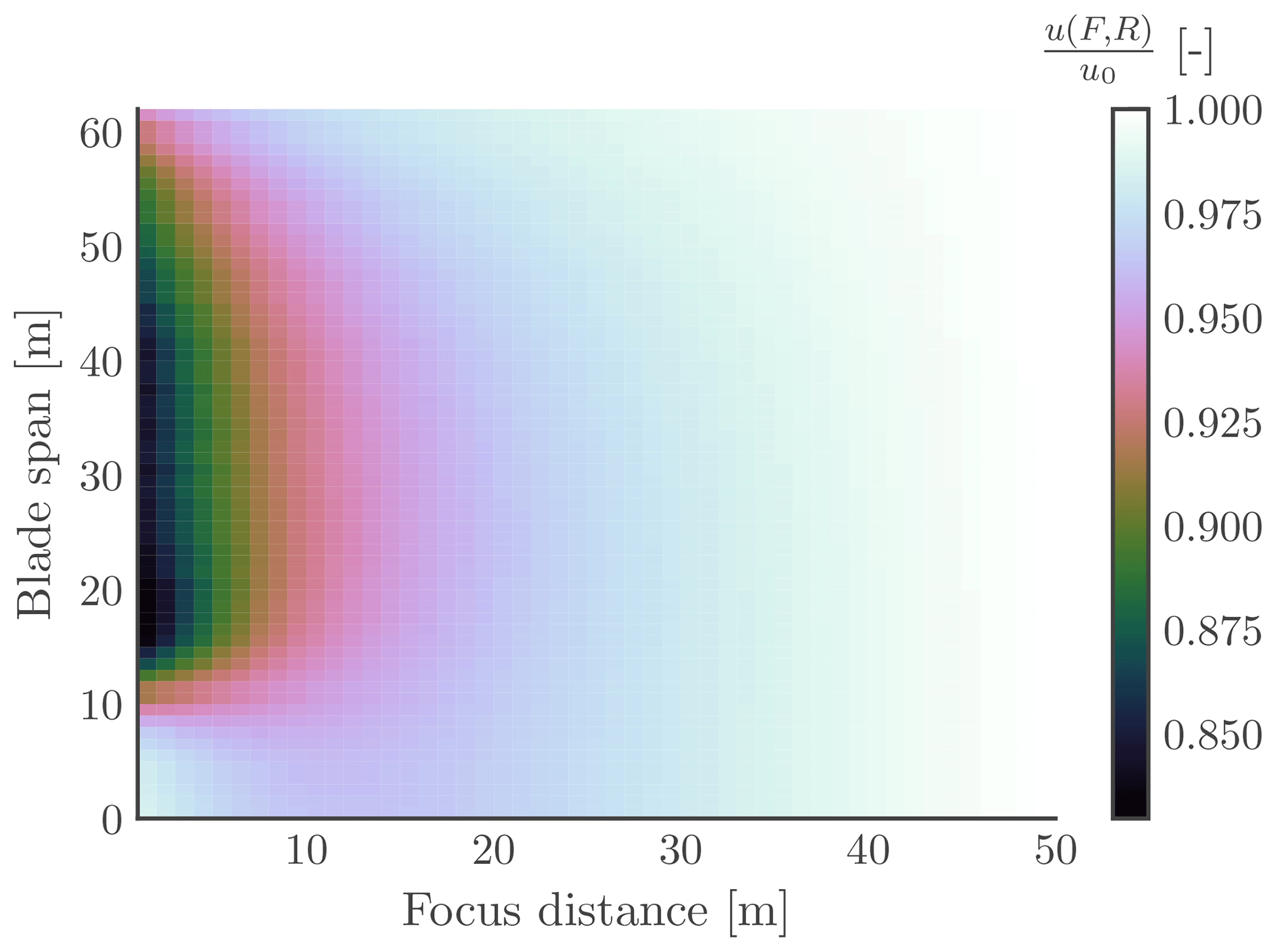
Figure 3 Normalized longitudinal inflow wind speed ($\frac{u(F,R)}{u_{\mathrm{0}}}$) as a function of focus distance (F) and blade span position (R), with an undisturbed inflow wind speed u₀=13 m s⁻¹.

Figure 3 illustrates the induction zone effect for laminar inflow. Note that the lidar measurement is affected by the rotor induction. The reduction depends on the position of the telescope along the blade radius (R) and the focus distance of the laser beam (F), where the wind speed measurement takes place. To account for this effect in the lidar-based inflow wind speed measurement, we construct a second-order polynomial function (f), whose inputs are chosen as rotor speed (ω_r), blade pitch angle (β_i), and blade root flapwise and edgewise moments (M_fw,i, M_ew,i). Rotor speed and blade pitch angles are easily measured, and we assume that blade root flapwise and edgewise moment sensors are also available for implementing this method. Therefore, the estimated wind speed parallel to the rotor shaft axis ($u_{\mathrm{h},\mathrm{est},i}$) is corrected as

$$\begin{array}{}\text{(5)}& u_{\mathrm{cor},i}=u_{\mathrm{h},\mathrm{est},i}+\mathrm{\Delta }{u}_{\mathrm{est},i},\end{array}$$

where

$$\begin{array}{}\text{(6)}& u_{\mathrm{0}}-u(F,R)\approx \mathrm{\Delta }{u}_{\mathrm{est},i}=f\left(F,R,{\mathit{\omega }}_{\mathrm{r}},{\mathit{\beta }}_i,M_{\mathrm{fw},i},M_{\mathrm{ew},i}\right).\end{array}$$

The second-order polynomial function (f) is fitted to the data extracted from 10 min large-eddy simulations with laminar inflow for mean wind speeds between 4 and 25 m s⁻¹. u(F, R) is the wind speed at an upstream distance F from the blade and at a blade radial position of R, and u₀ is taken from the same blade radial position of R but at an upstream distance of 3 times the rotor diameter (3-D).

2.3 Blade effective wind speed

To assess the performance efficiency of the blade-mounted lidar-based inflow wind speed measurement, we introduce a new signal called the blade-effective wind speed (u_beff,i), which is determined as the contribution of the inflow wind speed on each blade segment u_i(r) to the flapwise blade root bending moment; the inflow wind speed refers to the longitudinal wind speed in the rotor axis direction. The contribution depends on the radial distance (r) and the local thrust coefficient (C_T) of the blade segment as expressed by

$$\begin{array}{}\text{(7)}& u_{\mathrm{beff},i}=\sqrt{{\displaystyle \frac{\underset{R_{\mathrm{hub}}}{\overset{R_{\mathrm{tip}}}{\int }}{C}_{\mathrm{T}}\left(r,u_i\left(r\right)\right)r^{\mathrm{2}}{u}_i^{\mathrm{2}}\left(r\right)\mathrm{d}r}{\underset{R_{\mathrm{hub}}}{\overset{R_{\mathrm{tip}}}{\int }}{C}_{\mathrm{T}}\left(r,u_i\left(r\right)\right)r^{\mathrm{2}}\mathrm{d}r}}}.\end{array}$$

The local thrust coefficients are resolved from steady-state simulations for each blade segment from cut-in to cut-out wind speeds.

2.4 Multiblade coordinate transformation (MBC)

In the subsequent step, we introduce the multiblade coordinate transformation (MBC) that simplifies the controller design by transforming a time-varying system into a time-invariant system and decouples the individual pitch from the collective pitch control.

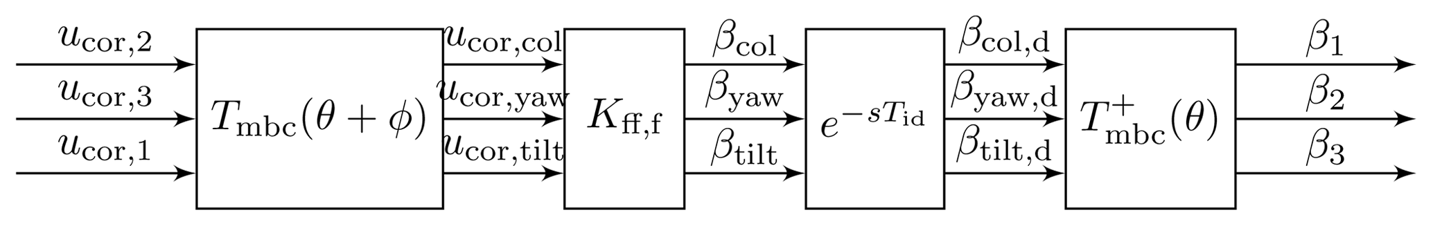
Figure 4 Implementation of the feedforward collective and individual pitch control, where the inputs (u_cor,1, u_cor,2, and u_cor,3) are the estimated wind speeds parallel to the rotor shaft axis and the outputs are the blade pitch angles (β₁, β₂, and β₃). The feedforward controller (K_ff,f) is implemented in the non-rotating (fixed) frame of reference and is, therefore, denoted with an extra index “f”. Further, the multiblade coordinate transformation (T_mbc) is applied to the inputs, and the pseudo-inverse transformation (${\mathbf{T}}_{\mathrm{mbc}}^{+}$) is applied to the outputs.

Figure 4 demonstrates the manner in which the feedforward controller is implemented. First, the measured inflow wind speed is transformed to the non-rotating frame of reference by applying MBC transformation (T_mbc(θ+ϕ)) in accordance with Eq. (8), where θ denotes the azimuth angle.

$$\begin{array}{}\text{(8)}& \left[\begin{array}{l}{u}_{\mathrm{cor},\mathrm{col}}\\ u_{\mathrm{cor},\mathrm{yaw}}\\ u_{\mathrm{cor},\mathrm{tilt}}\end{array}\right]={\mathbf{T}}_{\mathrm{mbc}}(\mathit{\theta }+\mathit{\varphi })\left[\begin{array}{c}{u}_{\mathrm{cor},\mathrm{2}}\\ u_{\mathrm{cor},\mathrm{3}}\\ u_{\mathrm{cor},\mathrm{1}}\end{array}\right],\end{array}$$

where

$$\begin{array}{}\text{(9)}& {\mathbf{T}}_{\mathrm{mbc}}\left(\mathit{\theta }\right)=\left[\begin{array}{ccc}\frac{\mathrm{1}}{\mathrm{3}}& \frac{\mathrm{1}}{\mathrm{3}}& \frac{\mathrm{1}}{\mathrm{3}}\\ \frac{\mathrm{2}}{\mathrm{3}}\cos \left(n_{\mathrm{h}}\mathit{\theta }\right)& \frac{\mathrm{2}}{\mathrm{3}}\cos \left(n_{\mathrm{h}}\left[\mathit{\theta }+\frac{\mathrm{2}\mathit{\pi }}{\mathrm{3}}\right]\right)& \frac{\mathrm{2}}{\mathrm{3}}\cos \left(n_{\mathrm{h}}\left[\mathit{\theta }+\frac{\mathrm{4}\mathit{\pi }}{\mathrm{3}}\right]\right)\\ \frac{\mathrm{2}}{\mathrm{3}}\sin \left(n_{\mathrm{h}}\mathit{\theta }\right)& \frac{\mathrm{2}}{\mathrm{3}}\sin \left(n_{\mathrm{h}}\left[\mathit{\theta }+\frac{\mathrm{2}\mathit{\pi }}{\mathrm{3}}\right]\right)& \frac{\mathrm{2}}{\mathrm{3}}\sin \left(n_{\mathrm{h}}\left[\mathit{\theta }+\frac{\mathrm{4}\mathit{\pi }}{\mathrm{3}}\right]\right)\end{array}\right].\end{array}$$

A phase shift (ϕ) is introduced into the transformation to consider that the measured inflow wind speed hits the wind turbine blade after this azimuth angle change. This value varies with respect to several parameters, including the selected focus distance, inflow wind speed, and rotor speed. The estimated wind speed parallel to the rotor shaft axis from blade 1 is used to determine the blade pitch control at blade 1; hence, the order of the estimated wind speeds parallel to the rotor shaft axis has changed to u_cor,2, u_cor,3, and u_cor,1. Further, the control signals or the blade pitch angles (β_col, β_yaw, β_tilt) are determined by the feedforward controller (K_ff,f). If the preview time provided by the lidar is greater than the time delay induced by the feedforward controller, an additional time delay ($e^{-s{T}_{\mathrm{id}}}$) is introduced into the system. Finally, the delayed control signals (β_col,d, β_yaw,d, and β_tilt,d) are transformed to the rotating frame of reference using the pseudo-inverse of the MBC transformation (${\mathbf{T}}_{\mathrm{mbc}}^{+}\left(\mathit{\theta }\right)$). The main structure of the feedforward individual pitch controller in Fig. 4 can be used in the feedforward trailing edge flap controller as well.

The MBC transformation plays a considerably important role because it can transform a frequency component of interest, such as 1P, 2P, or 3P (Bossanyi, 2003; van Engelen, 2006), to a low-frequency component, named 0P. It is dependent on the selected value of n_h in Eq. (9). For example, 1P will be transformed to 0P when n_h is specified as 1, and 2P will be transformed to 0P when n_h is specified as 2.

In this study, we focus on identifying the uncertainty weight that can be used during the feedback–feedforward individual and collective pitch control development with an objective to mitigate the 1P loads at the flapwise blade root bending moments and to enhance the rotor speed tracking. This indicates that by considering n_h as 1, the measured inflow wind speeds are transformed to the non-rotating frame of reference in Eq. (9), where the uncertainty weight identification is conducted. Further, the same methodology can be applied to identify the uncertainty weight for higher-harmonics control by selecting a larger integer value of n_h.

We have already mentioned that the measured inflow wind speeds are transformed to the non-rotating frame of reference by applying the MBC transformation. In order to assess the performance efficiency of the blade-mounted lidar-based inflow wind speed measurement, the blade effective wind speeds are also transferred to the non-rotating frame using the MBC transformation as follows

$$\begin{array}{}\text{(10)}& \left[\begin{array}{l}{u}_{\mathrm{bef},\mathrm{col}}\\ u_{\mathrm{bef},\mathrm{yaw}}\\ u_{\mathrm{bef},\mathrm{tilt}}\end{array}\right]={\mathbf{T}}_{\mathrm{mbc}}\left(\mathit{\theta }\right)\left[\begin{array}{c}{u}_{\mathrm{bef},\mathrm{1}}\\ u_{\mathrm{bef},\mathrm{2}}\\ u_{\mathrm{bef},\mathrm{3}}\end{array}\right],\end{array}$$

where T_mbc(θ) is defined in Eq. (9).

2.5 System modelling with uncertain lidar measurements

We use the blade-mounted telescopes to measure the disturbance, or the inflow wind speed in this case. Afterward, the three measurements are transformed into the non-rotating frame of reference where they are used as inputs to the feedforward individual and collective pitch controllers. Figure 5 illustrates the disturbance rejection controller set-up with uncertainty. Each block in the figure represents a three-input and three-output system with a three-by-three matrix transfer function.

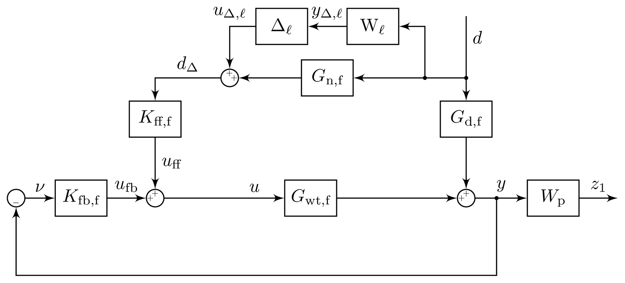
Figure 5 Block diagram of the disturbance rejection control design with performance weight and uncertain input measurement. K_fb,f and K_ff,f are the feedback and feedforward controllers, G_wt,f is the wind turbine model from the control input to output, G_d,f is the wind turbine model from the disturbance to the output, G_n,f is the nominal disturbance measurement model, Δ_ℓ is the uncertainty, W_ℓ is the measurement uncertainty weight, and W_p is the performance weight. The “f” in the index refers to the non-rotating (fixed) frame of reference.

The control development is aimed at achieving disturbance rejection up to a certain frequency with measurement uncertainties. In other words, we want to find a controller that satisfies Eq. (11) for a chosen performance weight W_p.

$$\begin{array}{}\text{(11)}& \parallel {\mathbf{W}}_{\mathrm{p}}{\mathbf{S}}_{\mathrm{fb}}{\mathbf{S}}_{\mathrm{ff},\mathrm{p}}{\parallel }_{\mathrm{\infty }}<\mathrm{1},\end{array}$$

where the frequency-dependent feedback (S_fb) and feedforward sensitivity (S_ff,p) functions with additive uncertainty are given by

$$\begin{array}{}\text{(12)}& {\displaystyle }& {\displaystyle }{\mathbf{S}}_{\mathrm{fb}}={\left(\mathbf{I}+{\mathbf{G}}_{\mathrm{wt},\mathrm{f}}{\mathbf{K}}_{\mathrm{fb},\mathrm{f}}\right)}^{-\mathrm{1}},\text{(13)}& {\displaystyle }& {\displaystyle }{\mathbf{S}}_{\mathrm{ff},\mathrm{p}}=\mathbf{I}+{\mathbf{G}}_{\mathrm{wt},\mathrm{f}}{\mathbf{K}}_{\mathrm{ff},\mathrm{f}}\left({\mathbf{G}}_{\mathrm{n},\mathrm{f}}+{\mathbf{\Delta }}_{\mathrm{\ell }}{\mathbf{W}}_{\mathrm{\ell }}\right){\mathbf{G}}_{\mathrm{d},\mathrm{f}}^{-\mathrm{1}},\end{array}$$

and

$$\begin{array}{}\text{(14)}& {\mathbf{\Delta }}_{\mathrm{\ell }}=\left[\begin{array}{ccc}{\mathit{\delta }}_{\mathrm{\ell },\mathrm{1}}& \mathrm{0}& \mathrm{0}\\ \mathrm{0}& {\mathit{\delta }}_{\mathrm{\ell },\mathrm{2}}& \mathrm{0}\\ \mathrm{0}& \mathrm{0}& {\mathit{\delta }}_{\mathrm{\ell },\mathrm{3}}\end{array}\right]\in {\mathbb{C}}^{\mathrm{3}\times \mathrm{3}},\parallel {\mathrm{\Delta }}_{\mathrm{\ell }}{\parallel }_{\mathrm{\infty }}\le \mathrm{1}.\end{array}$$

This equation highlights the importance of knowing the frequency-dependent uncertainty weight W_ℓ(jω) in advance, so as to ensure that the closed-loop system is stable and that the objective in Eq. (11) is satisfied for all perturbations ($\left|\right|{\mathbf{\Delta }}_{\mathrm{\ell }}|{|}_{\mathrm{\infty }}\le \mathrm{1}$). For control development, the frequency dependent uncertainty weight of W_ℓ(jω) and the nominal disturbance measurement model of G_n,f(jω) are missing; we discuss how they can be identified in the next subsections and later illustrate the process for the reference cases in Sect. 3.3.

Remark: only one objective is introduced in Eq. (11); nevertheless, other objectives can be added, such as penalizing the control signal magnitude at high frequencies (Ungurán et al., 2019).

2.6 Uncertainty modelling for control development

We employ black box system identification to establish the transfer functions (G_ℓ) from the blade effective wind speeds (u_beff) to the corrected lidar-based inflow wind speeds (u_cor) in the non-rotating (fixed) frame of reference

$$\begin{array}{}\text{(15)}& u_{\mathrm{cor},\mathrm{f}}={\mathbf{G}}_{\mathrm{\ell }}{u}_{\mathrm{beff},\mathrm{f}}\end{array}$$

with

$$\begin{array}{}\text{(16)}& {\mathbf{G}}_{\mathrm{\ell }}=\left[\begin{array}{ccc}{G}_{\mathrm{\ell },\mathrm{col}}& \mathrm{0}& \mathrm{0}\\ \mathrm{0}& G_{\mathrm{\ell },\mathrm{yaw}}& \mathrm{0}\\ \mathrm{0}& \mathrm{0}& G_{\mathrm{\ell },\mathrm{tilt}}\end{array}\right]\in {\mathbb{C}}^{\mathrm{3}\times \mathrm{3}}.\end{array}$$

The system identification is performed via the ssest function from MATLAB (2018) with a 15th-order state-space model, which can capture all the relevant information. The order of the state-space model is found empirically through analysis of the Hankel singular values.

We separately identify the nominal disturbance measurement model (G_n,k(j ω)) and the uncertainty weight (w_ℓ,k(jω)), where k∈{col, yaw, tilt}, as a fifth-order minimum phase filter for each of the inputs in such a way as to satisfy the following inequalities

$$\begin{array}{}\text{(17)}& \left|G_{\mathrm{n},k}\left(j\mathit{\omega }\right)\right|<\left|G_{\mathrm{\ell },k}\left(j\mathit{\omega }\right)\right|,\forall \mathit{\omega }\end{array}$$

and

$$\begin{array}{}\text{(18)}& \left|G_{\mathrm{n},k}\left(j\mathit{\omega }\right)+w_{\mathrm{\ell },k}\left(j\mathit{\omega }\right)\right|>\left|G_{\mathrm{\ell },k}\left(j\mathit{\omega }\right)\right|,\forall \mathit{\omega },\end{array}$$

leading to the diagonal nominal disturbance measurement model matrix of

$$\begin{array}{}\text{(19)}& {\mathbf{G}}_{\mathrm{n}}=\left[\begin{array}{ccc}{G}_{\mathrm{n},\mathrm{col}}& \mathrm{0}& \mathrm{0}\\ \mathrm{0}& G_{\mathrm{n},\mathrm{yaw}}& \mathrm{0}\\ \mathrm{0}& \mathrm{0}& G_{\mathrm{n},\mathrm{tilt}}\end{array}\right]\end{array}$$

and uncertainty weight matrix of

$$\begin{array}{}\text{(20)}& {\mathbf{W}}_{\mathrm{\ell }}=\left[\begin{array}{ccc}{w}_{\mathrm{\ell },\mathrm{col}}& \mathrm{0}& \mathrm{0}\\ \mathrm{0}& w_{\mathrm{\ell },\mathrm{yaw}}& \mathrm{0}\\ \mathrm{0}& \mathrm{0}& w_{\mathrm{\ell },\mathrm{tilt}}\end{array}\right].\end{array}$$

The order of the transfer functions are determined empirically during the analysis of the data. Lower orders could be selected as well; however, these would lead to higher uncertainties at high frequency.

The ideal case would be to measure, with a telescope, the exact inflow wind speed hitting the rotor blades to result in a nominal disturbance measurement transfer function with a gain of 1 over the entire frequency range. However, not only the inflow condition, but also the telescope parameters influence the nominal disturbance measurement model and the measurement uncertainty weight. In Sect. 3.3 we identify these transfer functions (G_n,k and w_ℓ,k), which can then be used for control development and analysis. Furthermore, we analyse how much the low-frequency gains of G_ℓ deviate from 1 for several cases.

We neglect the cross-coupling between the yaw and tilt components in the system identification, but these are considered in the wind turbine and disturbance transfer functions in line with Lu et al. (2015), so that the cross-coupling between the yaw and tilt components is included in the controller development.

2.7 Preview time estimation

Preview time plays an important role in the development of feedforward control. It must be larger than or equal to the time delay introduced by the feedforward controller and actuator dynamics. It is preferable for it to be equal, but a larger value is acceptable, as an additional time delay can be easily introduced into the feedforward controller, as shown in Fig. 4. To determine the optimal preview time for a given focus distance, we evaluate the cross-correlation between the blade effective (u_beff,k) and the corrected inflow (u_cor,k) wind speeds, with k∈{col, yaw, tilt}, and we choose the index of the peak value as the available preview time.

2.8 Telescope parameter estimation

We introduce a cost function which is based only on the coherence (${\mathit{\gamma }}_k^{\mathrm{2}}$) between the blade effective (u_beff,k) and the corrected inflow (u_cor,k) wind speeds, with k∈{col, yaw, tilt}:

$$\begin{array}{}\text{(21)}& J_{\mathrm{lp}}\left(f\right)=\sum _k{J}_{\mathrm{lp},k}\left(f\right)=\sum _k{\mathit{\gamma }}_k^{\mathrm{2}}\left(f\right).\end{array}$$

By evaluating J_lp for the discrete set of sampled lidar and telescope parameters, the maximum of the objective function results in the optimal telescope parameters within the discrete set of sampled lidar and telescope parameters. In this way, we are able to judge the initially chosen telescope parameters.

3 Results

3.1 Multiblade coordinate transformation effect on the blade-mounted lidar measurement

To perform an analysis of the MBC transformation, we create three generic wind speed measurement signals with

$$\begin{array}{}\text{(22)}& u_{\mathrm{cor},i}=u_{\mathrm{0}}+\sum _{j=\mathrm{1}}^{\mathrm{6}}{\displaystyle \frac{\mathrm{1}}{j^{\mathrm{3}}}}\sin \left(j\left[\mathrm{2}\mathit{\pi }{f}_{\mathrm{0}}t+(i-\mathrm{1}){\displaystyle \frac{\mathrm{2}\mathit{\pi }}{\mathrm{3}}}+{\displaystyle \frac{\mathit{\pi }}{\mathrm{6}}}\right]\right),\end{array}$$

where u₀, i, f₀, and t are the offset or undisturbed inflow wind speed, blade index, 1P frequency, and time, respectively. Here, we considered harmonics of up to 6P (j=1 … 6). Figure 6 shows an example time series of the generated signals.

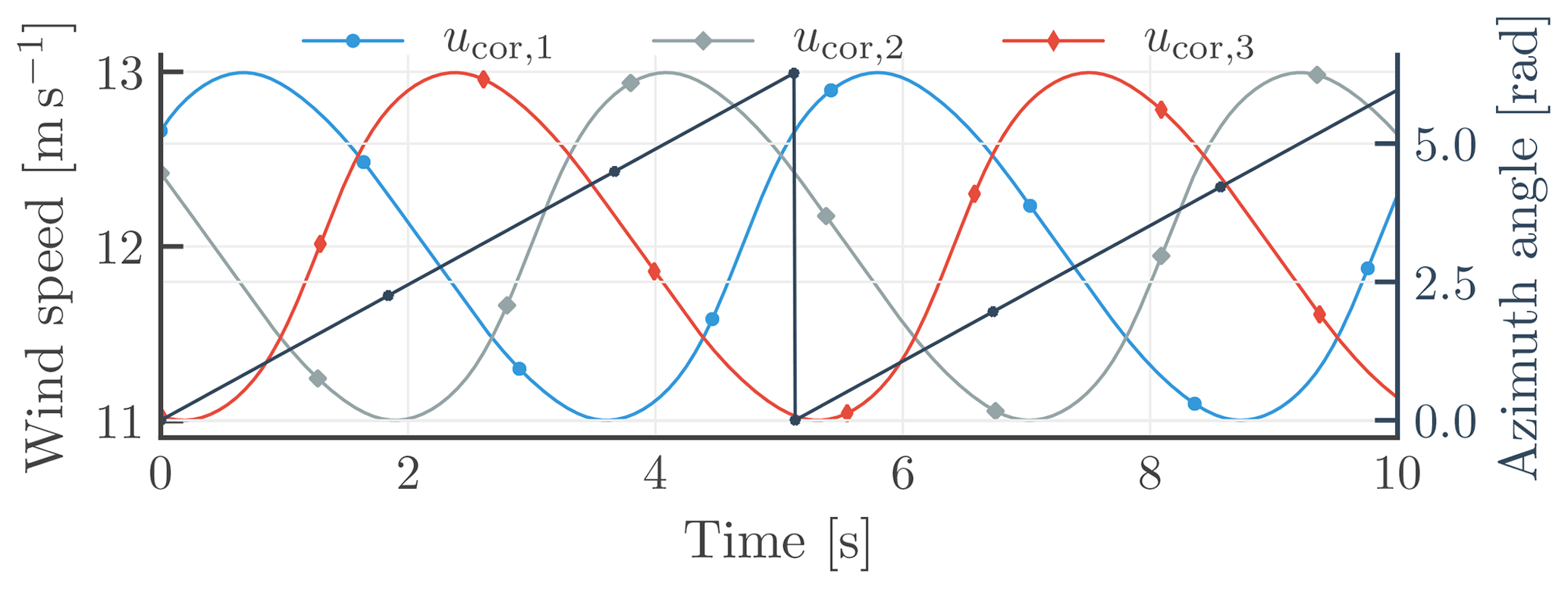
Figure 6 Time series of three generic wind speed measurements at the same amplitude, used for analysing the impact of the multiblade coordinate transformation. The first, second, and third signals have a phase shift of 30, 150, and 270^∘, respectively. The signals are constructed to include harmonics up to 6P.

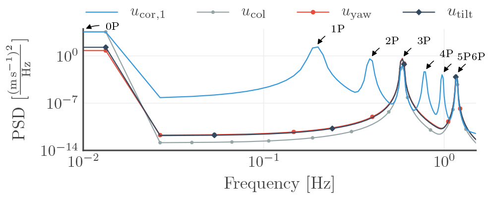
Figure 7 Power spectral densities of the generic signals in the rotating (u_cor,1) and non-rotating (u_col, u_yaw, u_tilt) frames of reference during the application of the multiblade coordinate transformation.

Figure 7 presents the power spectral densities of the wind speed measurement obtained from the first blade (u_cor,1) and the collective (u_col), yaw (u_yaw), and tilt (u_tilt) components after the MBC transformation, which is applied to the generic wind speed measurement signals (u_cor,1, u_cor,2, u_cor,3). The figure highlights the MBC transformation keeping only 0P, 3P, and multiples of 3P. As Lu et al. (2015) describe, the frequency (f) in the non-rotating frame of reference arises from f±f₀ from the rotating frame of reference; e.g. the 3P in the non-rotating frame of reference arises from the 2P and 4P contributions in the rotating frame of reference.

Several cases may illustrate the transfer of the measurement errors from the rotating to the non-rotating reference frame. First, we should consider the effect of over- or underestimation of the measured wind speed with one of the blade-mounted lidar systems, due to, e.g., different radial positions of the telescope along the blade radii or one of the telescopes having a different orientation, which reduces the DC offset (u₀ in Eq. 22) for one of the three generic signals. Next, the signals are transformed into the non-rotating frame of reference, which can be compared to the case where all the DC offsets are maintained for each of the three signals at the same level.

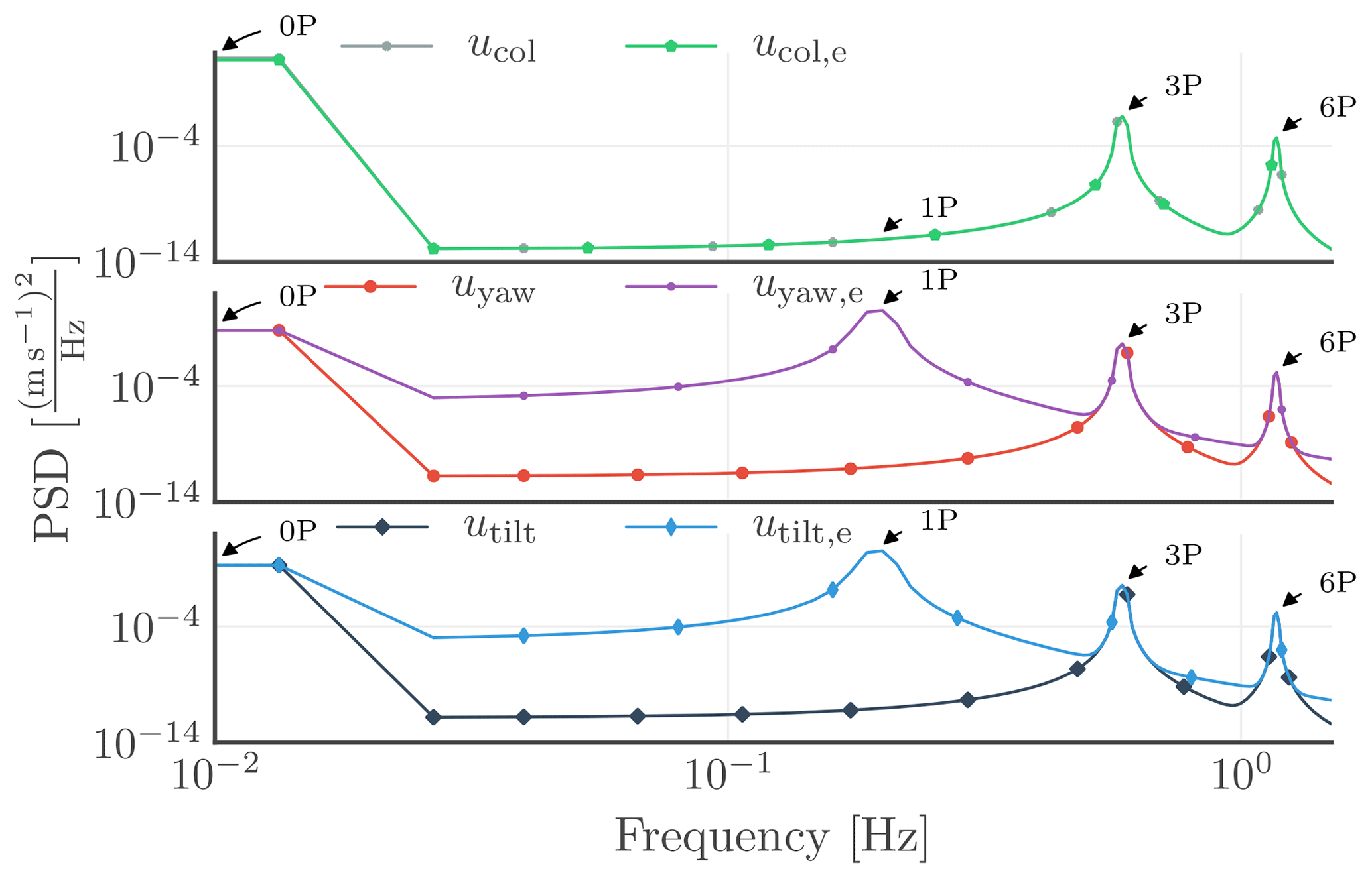
Figure 8 Power spectral densities of collective, yaw, and tilt components of the generic signals with partial DC offset. The expression u_…,e indicates the case where the DC offset (u₀ in Eq. 22) of one of the signals differs from the other two in the rotating frame of reference.

As Fig. 8 highlights, an undesired peak appears at 1P in the yaw and tilt components in the non-rotating frame of reference, due to the presence of asymmetries in the signals in the rotating frame of reference (Petrović et al., 2015).

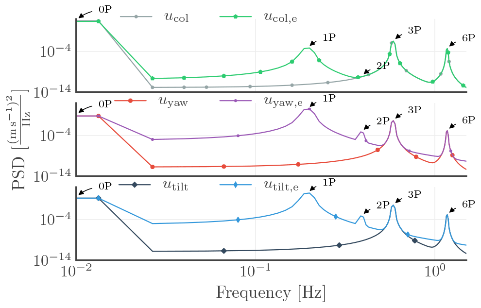
Figure 9 Power spectral densities of collective, yaw, and tilt components of the generic signals with partial DC offset and phase shift. The expression u_…,e indicates the case where a different DC offset is set and a 1^∘ phase shift is added to the 1P harmonics of one of the blade signals in the rotating frame of reference.

Second, in addition to the reduction in the DC offset for one of the signals, a 1^∘ phase shift is added to the 1P harmonic to the same signal in the rotating frame of reference, which represents the case, for example, where one of the blade-mounted lidar focus distances differs from the other two. Figure 9 reveals that after applying the MBC transformation to the three generic signals, undesired higher-harmonic peaks arise in the non-rotating frame of reference. Interestingly, the phase shift that is introduced to one of the signals in the rotating frame of reference results in different higher harmonics in the components in the non-rotating frame of reference, e.g. a peak observed at 1P of the collective component and both 1P at 2P of the tilt and yaw components.

3.2 Simulation set-up

The reference case we use in this investigation is based on the NREL 5 MW generic wind turbine (Jonkman et al., 2009). We use an actuator line model through the coupling between the FASTv7 aeroelastic simulation code (Jonkman and Buhl, 2005) and PALM (Parallelized Large-Eddy Simulation Model) (Maronga et al., 2015) as explained by Bromm et al. (2017). The operating conditions correspond to a hub-height mean wind speed of 13.06 m s⁻¹, which is above the rated value of 11.4 m s⁻¹. Furthermore, the 10 min simulation results in a turbulence intensity of 8.5 % and a wind shear corresponding to a power law description with an exponent of approximately 0.12. The baseline controller of the wind turbine ensures that the generator speed is kept at 1173.7 rpm (Jonkman et al., 2009), thereby resulting in a mean rotor speed (ω_r) of 11.74 rpm and further leading to a 1P frequency of f₀=0.195 Hz.

For an analysis of the induction zone effect, we set the range of the focus distance and telescope position along the blade radius at F∈[10, 40 m] and R∈[20, 60 m], based on a previous investigation (Ungurán et al., 2018). The range of the other input variables are determined by the results of simulations with laminar inflow and power law wind shear with coefficients of 0.1, 0.2, and 0.3. An approximation of the induction zone effect introduces some uncertainties into the measurement, but they are included in the identified uncertainty weight.

3.3 Nominal plants and uncertainty weights identification

Ungurán et al. (2019) stress that an elevated peak around the crossover frequency (just below the 1P frequency) of the feedback–feedforward controller sensitivity function leads to increased loads across the wind turbine components. Here, the crossover frequency of the controller is defined where the sensitivity function first crosses −3 dB from below. Uncertainties impose limitations on the achievable performance (Skogestad and Postlethwaite, 2005); e.g. the peak of the sensitivity function may increase due to uncertainties in the system. Therefore, it is important to analyse how the lidar measurement uncertainty is affected by, e.g., mounting misalignment of the telescope on the blade or cases where the focus distance or position of the telescope along the blade span differs from the optimal parameters. Identifying the lidar measurement uncertainty as a frequency-dependent minimum-phase filter enables the inclusion of such parameters in the control development, allowing an analysis of its impact on the stability and performance of the closed-loop system. As we explain in detail in Sect. 3.3.1, a straightforward solution to determine the telescope and lidar parameters, such as focus distance, telescope position along the blade radius, and telescope orientation on the blade, is to assume that the blades are rigid, that the rotor speed and pitch angle are constant, and that Taylor's frozen turbulence hypothesis (Taylor, 1938) holds (Ungurán et al., 2018). We perform large-eddy simulation (LES) in the subsequent sections to examine the usefulness and limitations of these assumptions and further analyse the uncertainties in the blade-mounted lidar measurement as well as the measurement sensitivity with respect to lidar and telescope parameter changes. The investigated cases are described in Sect. 3.3.1–3.3.5 and summarized in Table 1. Section 3.3.6 describes how the measurement uncertainties are affected when one or two telescopes are aligned differently than the others. First, we assume that the orientation angle misalignment is unknown. Second, we assume that this orientation angle misalignment can be identified, so that the lidar-based inflow wind speed measurement can be corrected.

Table 1 The cases investigated in this study, along with the lidar and telescope parameters for each case. If one or more parameters in the third column are not specified, then the parameters defined in the first case are used. F is the focus length, R is the radial position of the telescope along the blade, and Φ_ℓ,i and Γ_ℓ,i are the orientation angles of the telescope (see Fig. 2).

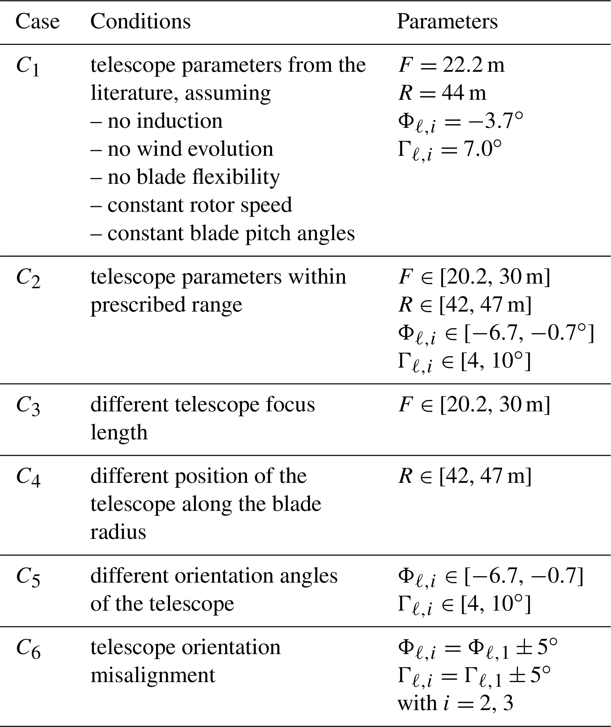
For each case, first the transfer functions (G_ℓ,k) from the blade effective wind speeds (u_beff,k) to the corrected lidar-based inflow wind speeds (u_cor,k) are identified. Next, the nominal disturbance measurement models (G_n,k) and the uncertainty weights (w_ℓ,k) for each of the inputs are estimated to satisfy Eqs. (17) and (18). Figure 10 provides a summary of the identified DC gain upper ($G_{\mathrm{n},k}+w_{\mathrm{\ell },k}$) and lower (G_n,k) bounds of the transfer functions (G_ℓ,k) from the blade effective wind speeds (u_beff,k) to the corrected lidar-based inflow wind speeds (u_cor,k).

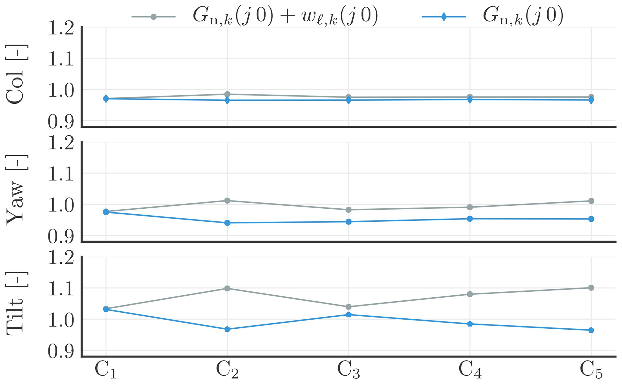
Figure 10 Identified DC gain upper ($G_{\mathrm{n},k}+w_{\mathrm{\ell },k}$) and lower (G_n,k) bounds of the transfer functions (G_ℓ,k) from the blade effective wind speeds (u_beff,k) to the corrected lidar-based inflow wind speeds (u_cor,k), with k∈{col, yaw, tilt}; C₁–C₅ represent the investigated cases (outlined in Table 1).

We would like to act only below the 1P (0.195 Hz) frequency; therefore, below this frequency, it is desired that the gain of G_n,k is 1 and that the measurement uncertainty is small but still covers the worst case. A higher percentage of measurement uncertainty can be tolerated at frequencies above 1P by designing the feedforward controller accordingly, e.g. a model inversion-based feedforward controller with a low-pass filter with a crossover frequency below 1P. With Fig. 10, we show how wide variation in the DC gain of G_ℓ,k agreed with the identified nominal disturbance measurement models and the additive uncertainty weights.

3.3.1 Telescope parameters for no-induction case (C₁)

The basic concept of the feedforward controller is the use of measured inflow wind speed from blade i to control the blade and trailing edge flap angles at blade i−1. Assuming rigid blades, constant rotor speed and pitch angle and that Taylor's frozen turbulence hypothesis (Taylor, 1938) holds, it is easy to compute the minimum preview time of 1.7 s ($=\frac{\mathrm{2}\mathit{\pi }}{\mathrm{3}}\frac{\mathrm{30}}{\mathit{\pi }{\mathit{\omega }}_{\mathrm{r}}}$, ω_r=11.74 rpm), which is the time needed for blade i−1 to reach the position of blade i, i.e. a 120^∘ azimuth angle change. The simulation set-up presented in Sect. 3.2 results in a hub-height mean wind speed of 13.06 m s⁻¹. The assumption that the wind evolves according to Taylor's frozen turbulence hypothesis and with the induction zone effect being negligible, a focus distance of 22.2 m (=1.7 s ⋅ 13.06 m s⁻¹) is determined. In accordance with Bossanyi (2013) and Simley et al. (2014a), the inflow at 70 % (≈44 m) of the blade radius can be assumed as most representative of the blade effective wind speed; hence, the telescope is located at this radial position. The telescope orientation angles Φ_ℓ,i and Γ_ℓ,i are found through aeroelastic simulation where laminar inflow is considered. The telescope orientation angles are the counter rotation of the blade segment angular orientation so that the lidar beam becomes parallel to the rotor shaft axis (see Fig. 2).

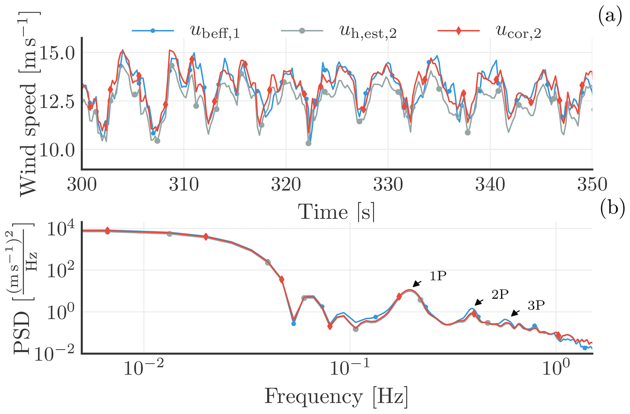
Figure 11 A selected time series of the blade effective wind speed from blade 1 (u_beff,1) and the estimated ($u_{h,\mathrm{est},\mathrm{2}}$) and corrected (u_cor,2) inflow wind speeds from blade 2 in the rotating frame of reference shown in (a). The power spectral densities (PSDs) of the three signals are displayed in the lower plot.

Figure 11a shows a selected time series of the blade effective wind speed from blade 1 (u_beff,1), as well as the estimated ($u_{\mathrm{h},\mathrm{est},\mathrm{2}}$) and corrected (u_cor,2) inflow wind speeds from blade 2. The three signals are in the rotating frame of reference. The lower plot displays the power spectral densities (PSDs) of the three signals. The dominant frequencies are clearly visible, as a result of the rotational sampling of the inflow wind speed by the blade-mounted telescope. The PSD analysis highlights these dominant frequencies as 1P, 2P, and 3P. Moreover, the plot reveals a good match at 1P between u_beff,1 and u_cor,2, although u_cor,2 is slightly underestimated at higher harmonics.

Figure 12 Power spectral densities of the blade effective wind speeds (u_beff,k) and the corrected inflow wind speeds (u_cor,k) in the non-rotating frame of reference, with k∈{col, yaw, tilt}.

We transform the different blade effective and corrected inflow wind speeds from the rotating to the non-rotating frame of reference via the multiblade coordinate transformation (T_mbc(θ)) as discussed in Sect. 2.4. Afterward, we evaluate the PSD for the collective, yaw, and tilt components of the signals, and the results are displayed in Sect. 12. The plot highlights the absence of 1P and 2P components (as observed in the rotating frame of reference; see Fig. 11) in the non-rotating frame of reference, in line with Sect. 2.4. Below 0.1 Hz, a good match between the collective and tilt components is observed, but the yaw component of the corrected inflow wind speed (u_cor,yaw) is slightly underestimated. Furthermore, the 3P component of u_cor,k (with k∈{col, yaw, tilt}) in the non-rotating frame of reference, which is the contribution of 2P and 4P from the rotating frame of reference, is likewise underestimated in all three components.

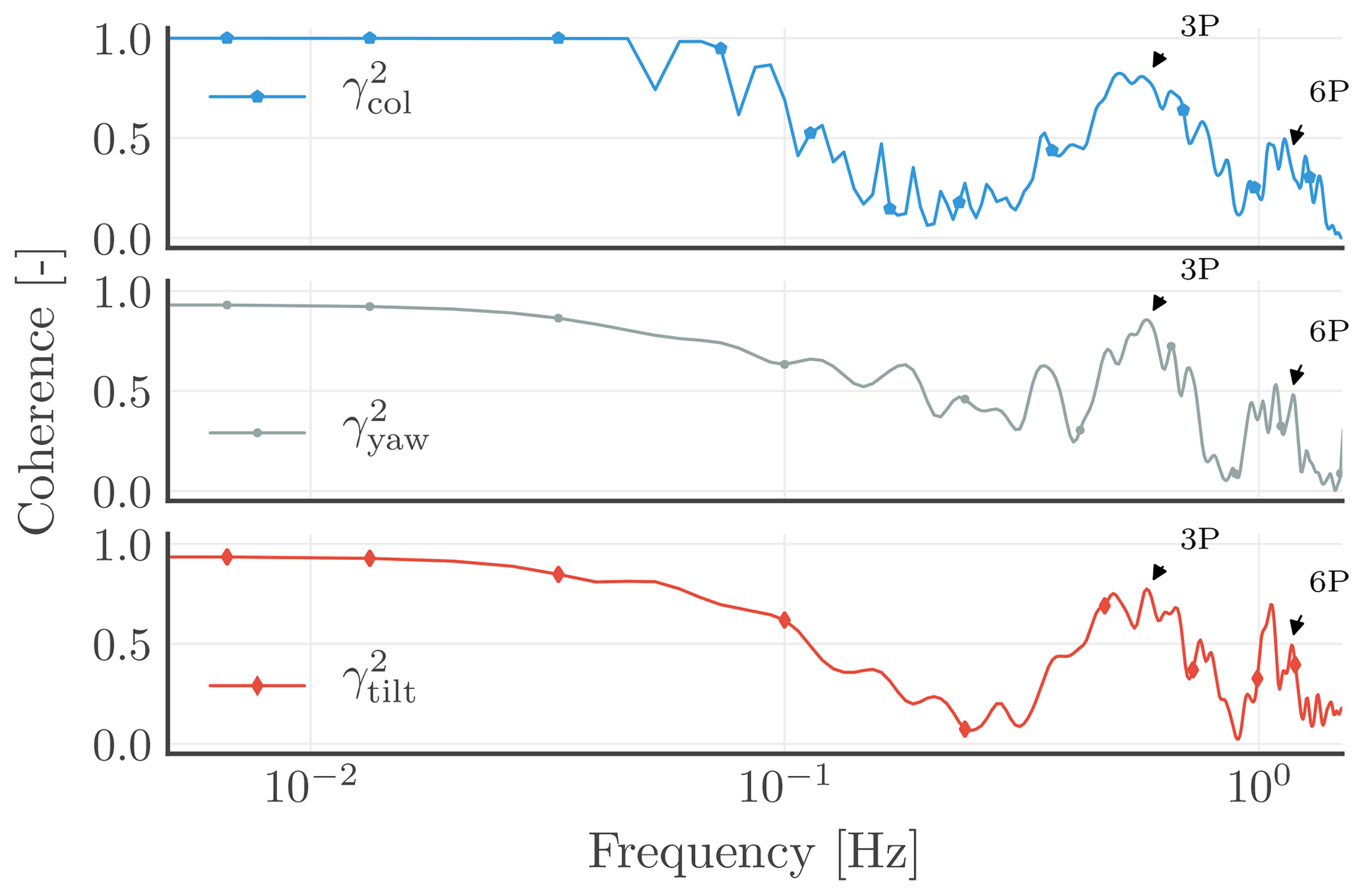
Figure 13 Coherences (γ²) between the blade effective wind speeds (u_beff,k) and the corrected inflow wind speeds (u_cor,k) in the non-rotating frame of reference, with k∈{col, yaw, tilt}.

Figure 13 reveals a good coherence at the frequencies where the power is concentrated, i.e. below 0.1 Hz, and at 3P and 6P. Additionally, the plots disclose the declining coherence with increasing frequency; i.e. higher coherence is achieved at 0P than at 3P; the same could be implied between 3P and 6P. With Fig. 12 highlighting the low-power content of the signals between 0P and 3P and between 3P and 6P, low coherences are similarly seen at the same frequencies in Fig. 13.

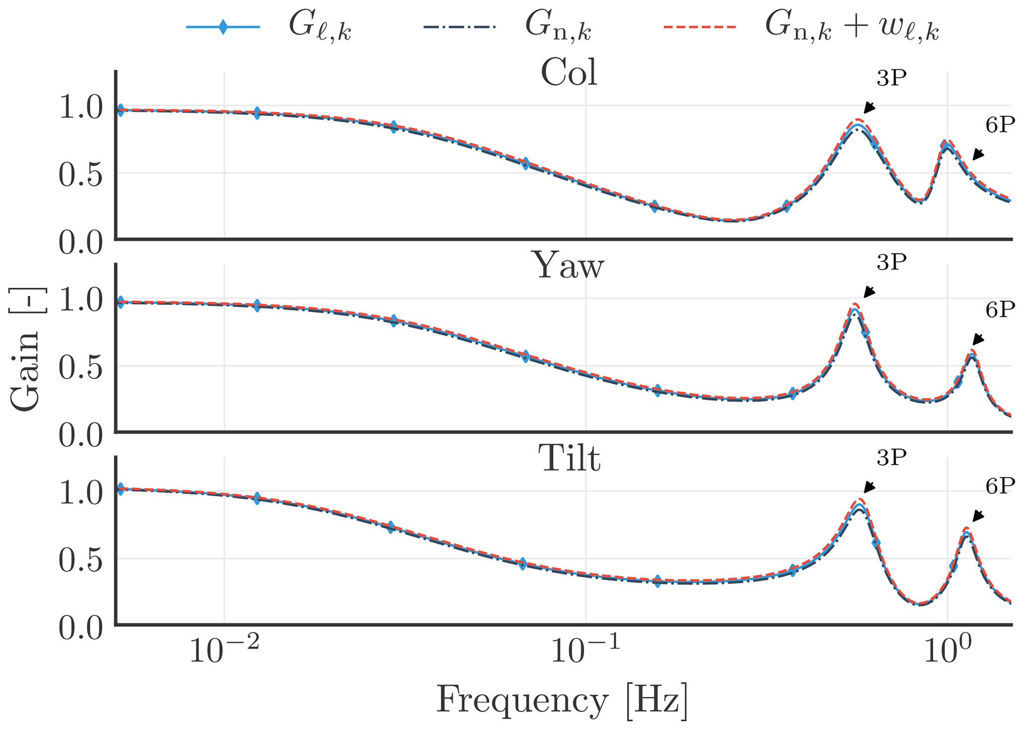
Figure 14 The identified disturbance measurement transfer functions (G_ℓ,k(j ω)). The dashed–dotted lines indicate the estimated nominal disturbance measurement models (G_n,k(jω)). The dashed lines show the sum of the estimated nominal disturbance measurement models and uncertainty weights ($G_{\mathrm{n},k}\left(j\mathit{\omega }\right)+w_{\mathrm{\ell },k}\left(j\mathit{\omega }\right)$), where k∈{col, yaw, tilt}.

Furthermore, we determine the disturbance measurement models (G_ℓ,k(jω)), the nominal disturbance measurement models (G_n,k(jω)), and the measurement uncertainty weights (w_ℓ,k(jω)), shown in Fig. 14, which can be incorporated into the feedback–feedforward individual pitch control development and analysis. This case is labelled as C₁ in Fig. 10. Figure 14 shows that this case only covers very small gain variations. The figure highlights that the mean value of the corrected inflow wind speed measurement is slightly underpredicted on the collective and yaw components, where the low-frequency gain is below 1, and is slightly overpredicted on the tilt component, where the low-frequency gain is above 1.

3.3.2 Uncertainties around the no-induction telescope parameters (C₂)

In this section, we investigate the impact on the uncertainty weights when the telescope parameters cannot be selected as defined for the no-induction case, but are close to these values. We carried out simulations involving a discrete set of sampled values for the focus distance, radial position of the telescope along the blade radii, and orientation angles of the telescope. The identified disturbance measurement transfer functions (G_ℓ,k(jω)) for the discrete set of sampled values are shown as overlapping blue lines in Fig. 15. The plot underscores that the disturbance measurement transfer functions are influenced by the telescope parameters. The low-frequency gain variation is different at each of the three components, which is also seen in Fig. 10, where it is labelled as C₂. The highest low-frequency gain variation is observed on the tilt component.

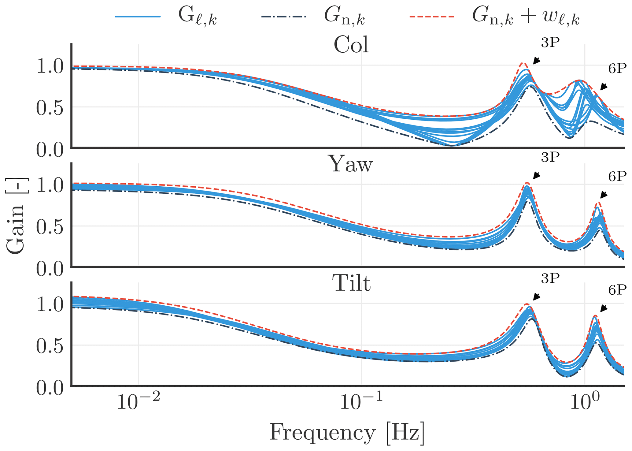
Figure 15 The identified disturbance measurement transfer functions (G_ℓ,k(jω)) for a discrete set of sampled telescope parameters. The dashed–dotted lines indicate the estimated nominal disturbance measurement models (G_n,k(jω)). The dashed lines show the sum of the estimated nominal disturbance measurement models and uncertainty weights ($G_{\mathrm{n},k}\left(j\mathit{\omega }\right)+w_{\mathrm{\ell },k}\left(j\mathit{\omega }\right)$), where k∈{col, yaw, tilt}.

3.3.3 Optimal focus distance and available preview time (C₃)

We determine the preview time in accordance with Sect. 2.7. We keep the telescope parameters constant as defined in Sect. 3.3.1, except for the focus distance, which is allowed to vary between 20.2 and 30 m. We determine a preview time of 1.9 s for all the focus distances, which is slightly higher than the initially calculated value of 1.7 s in Sect. 3.3.1.

This case is denoted as C₃ in Fig. 10, and that figure highlights that there is a smaller low-frequency gain variation for this case compared to the previous case (C₂).

3.3.4 Telescope position along the blade span (C₄)

Bossanyi (2013) proposed that a blade-mounted lidar placed at 70 % of the blade radius is most suitable for feedforward control input. We assess in this subsection whether placing the blade-mounted lidar at 70 % (≈44 m) of the blade radius would result in the maximum of the objective function in Eq. (21). We set f_max in Eq. (21) as 0.1 Hz, while we maintain a focus distance of 22.2 m.

We find that the telescope placed at a radial position of 46 m leads to the maximum value of the objective function in Eq. (21); in other words, the telescope positioned at a radial position of 46 m results in the highest coherence between the blade effective and the corrected inflow (u_cor,k) wind speeds. This corresponds to 73 % of the blade span. The value found is quite close to the findings of Bossanyi (2013). Varying the telescope radial position in a fairly small range (42–47 m) results in a higher low-frequency uncertainty in the tilt component than in the collective and yaw components (see C₄ in Fig. 10). In this case, at the yaw and tilt components, the low-frequency gain variation is higher than in C₃ but still smaller than in C₂.

3.3.5 Telescope orientation (C₅)

In this section, we evaluate whether the initially selected telescope orientation angles (Φ_ℓ,i and Γ_ℓ,i, with i=1, 2, 3) would result in a maximized objective function in Eq. (21). For this purpose, we fixed the telescope parameters as described in Sect. 3.3.1, with the exception of the orientation angles (Φ_ℓ,i and Γ_ℓ,i). The two angles are changed around the initially selected values. We simulate the lidar measurements with each new set of parameters.

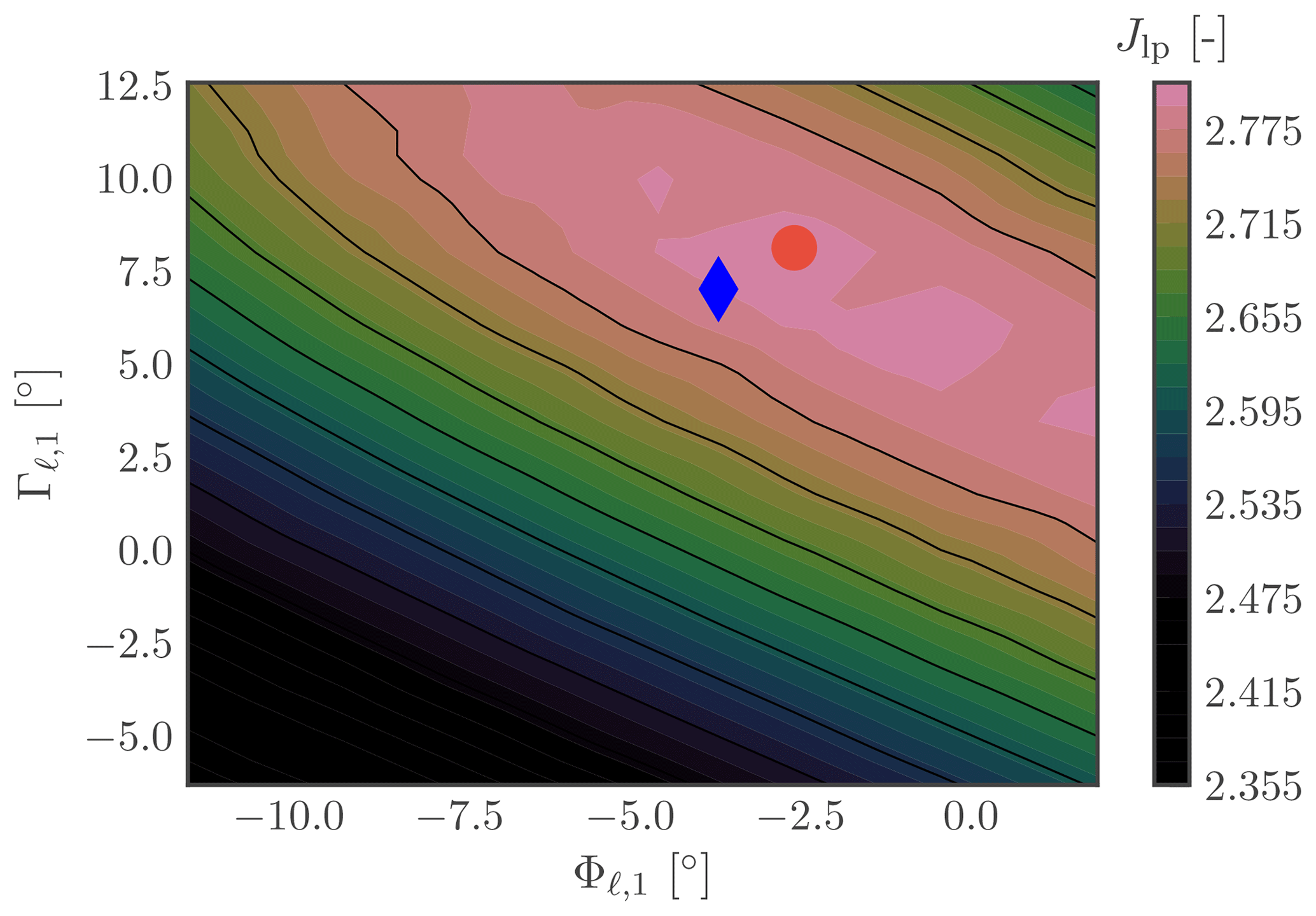
Figure 16 Optimal angular orientation of the telescope. The maximum frequency (f_max) in the objective function (J_lp) is set at 0.1 Hz. The blue diamond marks the parameters initially chosen; the red dot marks the maximum point of the function from Eq. (21).

We determine the optimal orientation of the telescope in Fig. 16 based on the objective function in Eq. (21). In the plot, the blue diamond marks the initial telescope orientation based on the no-induction calculation, where ${\mathrm{\Phi }}_{\mathrm{\ell },i}=-\mathrm{3.7}$^∘ and ${\mathrm{\Gamma }}_{\mathrm{\ell },i}=\mathrm{7.0}$^∘. The red dot indicates the obtained optimal value, where ${\mathrm{\Phi }}_{\mathrm{\ell },i}=-\mathrm{2.6}$^∘ and ${\mathrm{\Gamma }}_{\mathrm{\ell },i}=\mathrm{8.1}$^∘, which is only marginally different from the no-induction values.

The identified G_ℓ,k low-frequency (DC) gain upper   ($G_{\mathrm{n},k}\left(j\mathit{\omega }\right)+w_{\mathrm{\ell },k}\left(j\mathit{\omega }\right)$) and lower (G_n,k) bounds are labelled as C₅ in Fig. 10. This case results in similar low-frequency gain variations as C₂ at the yaw and tilt components; however, it has a smaller gain variation in the collective component than C₂.

3.3.6 Telescope orientation misalignment (C₆)

In this subsection, transfer functions (G_ℓ,k) from the blade effective wind speeds (u_beff,k) to the corrected lidar-based inflow wind speeds (u_cor,k) are identified for the cases where one or two of the telescopes have been aligned differently relative to their values in the no-induction case (C₁). Such cases could occur, for example, during telescope installation. Initially, we assume this misalignment is unknown but detectable to allow for a correction of the lidar-based inflow wind speed measurement. To simulate these cases, we fixed the telescope parameters as described in Sect. 3.3.1, except for the orientation angles of Φ_ℓ,i and Γ_ℓ,i of the telescopes mounted on the second and third blades. The angular values are changed around the no-induction values by ±5^∘ (${\mathrm{\Phi }}_{\mathrm{\ell },i}={\mathrm{\Phi }}_{\mathrm{\ell },\mathrm{1}}\pm \mathrm{5}$^∘ and ${\mathrm{\Gamma }}_{\mathrm{\ell },i}={\mathrm{\Gamma }}_{\mathrm{\ell },\mathrm{1}}\pm \mathrm{5}$^∘ for i=2, 3) as follows. First, the values are changed only for the telescope mounted on the second blade, then for the telescopes mounted on both the second and third blades.

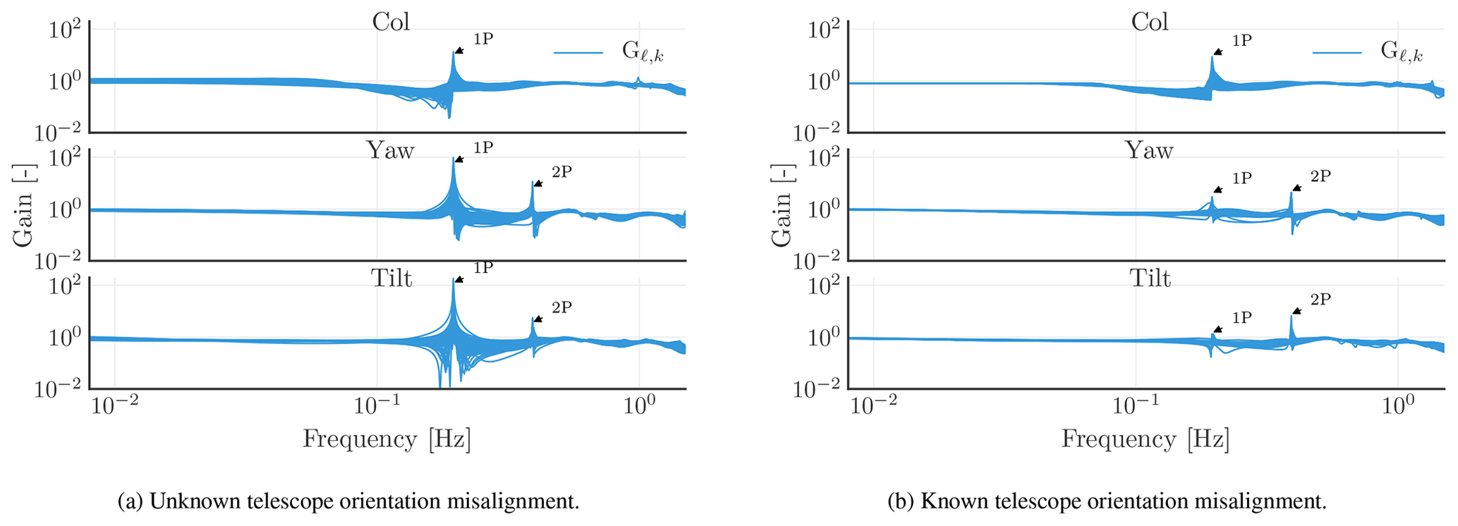
Figure 17 Identified transfer functions (G_ℓ,k) from the blade effective wind speeds (u_beff,k) to the corrected lidar-based inflow wind speeds (u_cor,k) for the discrete set of sampled telescope parameters with unknown and known telescope orientation misalignment, where k∈{col, yaw, tilt}.

We evaluate such a set-up via simulations. Figure 17a displays the identified transfer functions (G_ℓ,k) from the blade effective wind speeds (u_beff,k) to the corrected lidar-based inflow wind speeds (u_cor,k). Figure 17b reveals a 1P peak at the collective component and 1P and 2P peaks at the yaw and tilt components. As shown in Sect. 3.1, adding a phase shift of 1^∘ to the 1P harmonic and reducing the DC offset for one of the signals in the rotating frame of reference results in such undesired higher-harmonic peaks at the collective, yaw, and tilt components in the non-rotating frame of reference. Figure 17b underlines that, by assuming that the misalignment angles are identifiable and that the lidar-based inflow wind speed measurement is corrected accordingly, the undesired peak at 1P is reduced by a factor of 10, although existent on all the components.

4 Discussion

We have shown that the determined telescope parameters with assumptions of rigid blades, constant rotor speed and pitch angle, absence of induction, and Taylor's frozen turbulence hypothesis provide a good trade-off between simplicity and accuracy (see C₁ in Fig. 10). First, the low-frequency gains of the identified disturbance measurement models (G_ℓ,k(j ω)) only have small absolute deviations from 1, which are found to be 3 %, 2.5 %, and 3.1 % for collective, yaw, and tilt components, respectively. Second, the optimal telescope parameters in C₄ and C₅, which maximize a cost function based on the coherence between the blade effective (u_beff,k) and the corrected inflow (u_cor,k) wind speeds, are close to the telescope parameters in C₁. Such a small deviation is expected with respect to the assumptions we made during the calculation of the values for the no-induction case (see Sect. 3.3.1).

By evaluating the cross-correlation between the blade effective (u_beff,k) and the corrected inflow (u_cor,k) wind speeds for a discrete set of sampled values of the focus distance in Sect. 3.3.3, we found that the preview time is constant for all the selected focus distances. It is closely coupled to the time needed for blade i−1 to reach the position of blade i, i.e. 120^∘ azimuth angle change. For example, by considering laminar inflow with wind shear, no matter what the focus distance is, the delay time between the corrected inflow wind speed from blade 1 and the blade effective wind speed from blade 3 will always be the same, which is the time needed for blade i−1 to reach the position of blade i. If the focus distance has changed, the ϕ in the MBC transformation also has to be changed; furthermore, the control signal should be delayed accordingly. Note that control development must proceed with sufficient attention so as to ensure that the feedforward controller does not result in a higher time delay than the available preview time. For example, a feedforward controller with a crossover frequency of 0.1 Hz may result in higher time delay compared to that with a crossover frequency of 0.2 Hz (Dunne and Pao, 2016). With this, we want to point out that the feedforward controller crossover frequency and the focus distance are coupled. Hence, defining the former typically leads to a minimal selectable focus distance.

As stated above, the lidar and telescope parameters based on the assumptions we made in Sect. 3.3.1 provide a good trade-off between simplicity and accuracy. They are close to the optimal parameters we found for the discrete set of sampled values of the focus distance, the radial position of the telescope along the blade, and the orientation angles of the telescope in Sect. 3.3.3–3.3.5. Nevertheless, this is not the case for the preview time; the available preview time is slightly increased from 1.7 to 1.9 s, as we demonstrated in Sect. 3.3.3. This could be due to the assumptions we made: (a) the blades are rigid; (b) constant rotor speed and blade pitch angle; (c) Taylor's frozen turbulence hypothesis holds; and (d) the induction effect is absent during our calculation in Sect. 3.3.1. Furthermore, the signals were sampled with a sampling time of 0.2 s, which also imposes limitations on the resolution of the preview time. Note that LES simulations with lower sampling time are resource and time expensive. The crossover frequency of the feedforward controller affects the time delay. With a higher preview time available, we can select a lower crossover frequency. This understanding gives us more room during the feedback–feedforward control development. The available preview time could be determined online in field tests and used to delay the feedforward control signal accordingly. This can be done online by, for example, storing 10 min of blade effective (u_beff,k) and corrected inflow (u_cor,k) wind speed measurements and evaluating the cross-correlation between them.

We found that the blade-mounted lidar placed at the 73 % span of the blade radius results in the best coherence between the corrected inflow wind speed and the blade effective wind speed. This finding is close to the value (70 % of the blade radius) found by Bossanyi (2013) for a blade-mounted lidar and Simley et al. (2014a) for a hub-mounted lidar system.

Any unknown orientation angle misalignment for one of the telescopes leads to an unknown contribution of the rotational speed to the lidar-based line-of-sight wind speed measurement. This is the reason why the low-frequency gain can vary between 0.7 and 1.2. Nevertheless, this can be reduced to a low-frequency gain variation between 0.96 and 0.98 by assuming that we are able to detect the angular offset. By detecting the angular offset, we are able to better estimate what is the mean value of the blade effective wind speed, and the resulting G_ℓ,k low-frequency gain lower bound is 0.96, which is very close to 1. In addition, an undetected misalignment of the telescope orientation angle results in a phase shift of the 1P harmonic and a reduction or increase in the DC offset of the signal in the rotating frame of reference. This subsequently leads to undesired peaks at 1P and 2P frequencies at the collective, yaw, and tilt components in the non-rotating frame of reference. Assuming the angular offsets to be known, we can reduce 1P and 2P peaks by a factor of 10 for both yaw and tilt components, but we cannot completely eliminate them. Thus, the question as to whether robust stability and performance can be ensured with such peaks still remains. To avoid such a peak, the telescopes need to be well aligned with each other and the blade segment orientation angles and linear velocities should be measured well. We showed in Sects. 3.1 and 3.3.6 that an unknown orientation angle misalignment leads to a 1P peak at the yaw and tilt components in the frequency domain. Therefore, the orientation angles of the telescope can be identified by formulating an optimization problem, whose main objective is to minimize the 1P peaks at the yaw and tilt components, with the orientation angles of the telescopes as the decision variables.

The nominal measurement transfer functions and uncertainty weights identified for the no-induction case can be directly included in robust feedback–feedforward individual pitch and trailing edge flap control development to guarantee robust stability and performance. However, this would be a very optimistic approach, as we considered only one reference wind turbine with a single inflow wind condition, and we need to assess how the measurement uncertainties change for other wind turbines with different wind speeds, turbulence intensities, yaw misalignments, etc. The nominal measurement transfer functions and uncertainty weights found in Sect. 3.3.2 might cover these cases and may be better for robust control development. C₂ covers a wide range of telescope parameter variations; hence, if for some reason one or more lidar and telescope parameters cannot be selected as for the no-induction case but are close to these values, the established transfer functions from C₂ can be used for robust feedback–feedforward control development. In addition, C₂ also covers the situations where the mean blade pitch angle is increased or decreased due to the wind turbine operating at a different point. The final selection of the nominal measurement transfer functions and uncertainty weights depends on whether the lidar and telescope parameters are varied dynamically with the operating points of the wind turbine and the wind speed or are kept constant over the entire operating range. Nevertheless, this may result in a conservative feedforward controller, thus limiting the benefits of the lidar system.

The methodology we presented in this paper can be applied in identifying the uncertainty weight for higher-harmonics control development; i.e. selecting n_h as 2 in Eq. (8) can be used to identify the uncertainty weight for the controller to mitigate 2P dynamic blade loads.

5 Conclusions

Our paper has aimed to identify the nominal measurement transfer functions and model the uncertainties in blade-mounted lidar measurements as a frequency-dependent uncertainty weight for inclusion into the feedback–feedforward individual pitch and trailing edge flap control development.

We found that the preview time with the lidar mounted on the blade is more linked to the time it takes the previous blade to reach the position of the blade from which the measurement took place rather than the focus distance. For a given focus distance, the preview time can be estimated online; hence, the feedforward control signal can be delayed accordingly. While the selected focus distance should provide sufficient preview time, it is desirable that the time delay introduced by the feedforward controller and actuators be eliminated. This sets the lower limit for the selectable focus distance.

Accordingly, we introduced a simple method, based on steady-state data, to calculate the telescope and lidar parameters. Nevertheless, we showed in a large-eddy simulation that such an approach provides a good trade-off between an efficient determination of the telescope parameters and accurate inflow wind speed measurement. The low-frequency gains of identified disturbance measurement transfer functions had small absolute deviations from 1, which were due to wind evolution, the cyclops dilemma, using a single-point measurement to estimate the blade effective wind speed, and the assumptions we made to correct the measurements. The nominal measurement transfer functions and uncertainty weights, as we have identified in this paper for several cases, can be directly included in the robust feedback–feedforward individual pitch and trailing edge flap control development to ensure robust stability and performance. However, to prevent the transfer functions (G_ℓ) from the blade effective wind speeds (u_beff) to the corrected lidar-based inflow wind speeds (u_cor) from having a large high-frequency gain at 1P and 2P in the non-rotating frame of reference, the telescopes must be well aligned with each other and the blade segment orientation angles and linear velocities should be measured well.