Optimal closed-loop wake steering – Part 1: Conventionally neutral atmospheric boundary layer conditions

Strategies for wake loss mitigation through the use of dynamic closed-loop wake steering are investigated using large eddy simulations of conventionally neutral atmospheric boundary layer conditions in which the neutral boundary layer is capped by an inversion and a stable free atmosphere. The closed-loop controller synthesized in this study consists of a physics-based lifting line wake model combined with a data-driven ensemble Kalman filter (EnKF) state estimation technique to calibrate the wake model as a function of time in a generalized transient atmospheric flow environment. Computationally efficient gradient ascent yaw misalignment selection along with efficient state estimation enables the dynamic yaw calculation for real-time wind farm control. The wake steering controller is tested in a six-turbine array embedded in a statistically quasi-stationary, conventionally neutral flow with geostrophic forcing and Coriolis effects included. The controller statistically significantly increases power production compared to the baseline, greedy, yaw-aligned control provided that the EnKF estimation is constrained and informed with a physics-based prior belief of the wake model parameters. The influence of the model for the coefficient of power C_p as a function of the yaw misalignment is characterized. Errors in estimation of the power reduction as a function of yaw misalignment are shown to result in yaw steering configurations that underperform the baseline yaw-aligned configuration. Overestimating the power reduction due to yaw misalignment leads to increased power over the greedy operation, while underestimating the power reduction leads to decreased power; therefore, in an application where the influence of yaw misalignment on C_p is unknown, a conservative estimate should be taken. The EnKF-augmented wake model predicts the power production in yaw misalignment with a mean absolute error over the turbines in the farm of 0.02P₁, with P₁ as the power of the leading turbine at the farm. A standard wake model with wake spreading based on an empirical turbulence intensity relationship leads to a mean absolute error of 0.11P₁, demonstrating that state estimation improves the predictive capabilities of simplified wake models.

1 Introduction

Modern horizontal axis wind turbines achieve performance approaching the Betz limit (Wiser et al., 2015). However, collections of wind turbines arranged in wind farms suffer from aerodynamic interactions which reduce wind farm power production by between 10 % and 20 % (Barthelmie et al., 2009) due to greedy control schemes which only consider the power maximization of individual wind turbines at the farm. Recent work has focused on the operation of wind turbines in a collective fashion in order to increase the power production of the wind farm through the mitigation of wake interactions (see review by Boersma et al., 2017).

Wind farm power optimization through wake interaction mitigation methods has generally relied on axial induction and yaw misalignment control since these two methodologies do not require significant hardware modifications on traditional horizontal axis wind turbines (Burton et al., 2011). Readers are directed to Knudsen et al. (2015) and Kheirabadi and Nagamune (2019) for recent reviews of wind farm power maximization methodologies. Previous simulation studies have shown that wake steering may have more potential than static axial induction control for wind farm power maximization (Annoni et al., 2016; Gebraad et al., 2016a; Campagnolo et al., 2016), although dynamic axial induction (Park and Law, 2016; Munters and Meyers, 2018; Frederik et al., 2020) or more sophisticated dynamic blade pitch strategies (Frederik et al., 2019) may significantly increase power production and require future field experimentation.

Greedy wind turbine operation minimizes the yaw misalignment between the nacelle position and the incoming wind direction. Contemporary wind turbines often operate in small yaw misalignment due to sensor noise and uncertainty (Fleming et al., 2014) leading to suboptimal power production for the misaligned turbine. However, recent attention has focused on wake steering, which is the intentional misalignment of certain turbines within a wind farm in order to deflect wakes laterally away from downwind generators (Grant et al., 1997; Jiménez et al., 2010). While the yaw-misaligned wind turbine's power production is decreased (Medici, 2005; Burton et al., 2011), wake steering has been shown to increase the power production of downwind generators in simulations (Fleming et al., 2016; Gebraad et al., 2017; Fleming et al., 2018; Archer and Vasel-Be-Hagh, 2019) and wind tunnel experiments (Adaramola and Krogstad, 2011; Mühle et al., 2018; Bastankhah and Porté-Agel, 2019). Further, the potential for wake steering to increase wind farm power production in wind conditions with wake losses has been observed in full-scale field campaigns with two (Fleming et al., 2017, 2019) and six wind turbines (Howland et al., 2019).

While wake steering has been shown to be a beneficial global wind farm control strategy compared to the greedy operation, the selection of the optimal yaw misalignment strategy for each wind turbine at a farm is challenging. The optimal yaw misalignment angles depend on the wake interactions between wind turbines (Gebraad et al., 2017). These wake interactions are dependent on wind speed, wind direction, atmospheric stability, turbulence intensity, local terrain, and other flow features (see, e.g., Hansen et al., 2012). Most wake steering control strategies have relied on static engineering wake models such as the Flow Redirection and Induction in Steady-state (FLORIS) model (Gebraad et al., 2016a, b; Fleming et al., 2016) or a lifting line model (Shapiro et al., 2018; Howland et al., 2019) to select the optimal yaw misalignment strategy based on a steady, time-averaged assumption of the wind farm flow. However, these static model approaches may have challenges in establishing the optimal yaw misalignment strategy as a function of time in a transient flow environment such as the stable atmospheric boundary layer (ABL) or the full diurnal cycle (see, e.g., Wyngaard, 2010).

Recent work has focused on the selection of the optimal yaw misalignment angles as a function of time for transient flow applications. Ciri et al. (2017) used a model-free formulation and dynamic control to increase the power production of a model wind farm in simulations. While model-free optimization is the subject of promising ongoing work, this methodology generally experiences slower rates of convergence and may be less suited to transient flow applications where wind conditions shift rapidly, although future work should compare model-based and model-free formulations in transient flow applications. A significant challenge in transient flow environments is in accurately predicting the power production given the greedy baseline control when considering ABL and controller state uncertainty in a utility-scale wind farm. The ensemble Kalman filter (EnKF) has been leveraged to perform model state estimation as a function of time (Doekemeijer et al., 2017) and for low-order model state estimation for the purpose of receding horizon frequency regulation control (Shapiro et al., 2017) and reference power signal tracking applications (Shapiro et al., 2019). Doekemeijer et al. (2018) found that the EnKF has comparable state estimation performance given either nacelle-mounted lidar data or supervisory control and data acquisition (SCADA) power production data alone. Since very few utility-scale wind turbines have nacelle-mounted lidar systems, the successful performance of the EnKF based on SCADA data alone highlights the potential for online model calibration without additional hardware installation.

Static wake-model-based dynamic control studies have utilized a quasi-static wake steering approach wherein the optimal yaw misalignment angles are computed and stored as a function of wind speed and direction based on static wake models with predefined model parameters (Fleming et al., 2019). However, the predefined model parameters were calibrated for the Gaussian wake model (Bastankhah and Porté-Agel, 2014) based on idealized large eddy simulations (LESs), and their applicability to a new utility-scale field implementation are unknown a priori. Further, there is additional uncertainty associated with the freestream velocity and turbulence intensity measurements in a wind farm environment where the typical sensors are limited to nacelle-mounted anemometers placed directly behind the rotating rotor. The dynamic influence of yaw misalignment on these sensors is unknown (Howland et al., 2019). Recently, Raach et al. (2019) used the FLORIS wake model to design a closed-loop wake steering controller which relies on a downwind facing nacelle-mounted lidar system which was able to increase power production in an example of a nine wind turbine LES case. In order to focus on a low-order methodology which does not require additional hardware installation, we develop a closed-loop, wake-model-based wake steering control for the application of data-driven wind farm power maximization based on SCADA power production data. The algorithm was designed for real-time control of utility-scale wind turbines without the requirement of additional hardware or sensor measurement systems, and it utilizes the gradient-based optimal yaw algorithm developed by Howland et al. (2019). The dynamic wake steering controller implemented in this study does not require historical data to be sorted into preselected wind speed and direction bins in order to make optimal yaw misalignment decisions. This is beneficial since the sorting of SCADA data represents a major uncertainty associated with wake steering control (Fleming et al., 2019; Howland et al., 2019).

Analytic wake models require a number of simplifications of the flow physics and wind turbine operation in order to predict wind farm power production in a computationally efficient fashion (see, e.g., review by Stevens and Meneveau, 2017). However, compared to model-free control, the wake model encodes a prior belief of the physics of wind farm flows and establishes a base performance given the initial model parameters preceding the perturbations applied by the EnKF (also see discussion by Schreiber et al., 2020). The selected model-based optimal yaw misalignment angles will depend on the wake deflection model form and parameters, and the model for power production degradation as a function of the yaw misalignment angle. Further, in a low-order, model-driven power optimization application, the selected yaw misalignment angles will depend on the wind farm layout, wind direction and speed, and stability state of the ABL. The goal of the present study is to analyze the sensitivity of wind farm power production to the design of the control system, model for power loss as a function of yaw misalignment, and wind farm layout when leveraging wake steering control.

This work represents Part 1 of the results and targets a canonical planetary boundary layer with conventionally neutral stratification. Part 2 will focus on a sensitivity analysis of wake steering control with temporally varying stratification and surface heat flux. Section 2 will introduce the dynamic wake steering methodology and EnKF state estimation technique. The LES methodology is introduced in Sect. 3. In Sect. 4, the sensitivity to model architecture and parameters is tested in LES of the conventionally neutral ABL with realistic Coriolis forcing. Finally, conclusions are given in Sect. 5.

2 Dynamic wake steering methodology

The present methodology is focused on optimal closed-loop wake steering control as a function of time for transient flow applications. The dynamic wake steering controller is illustrated in Fig. 1. The controller entails a forward-pass wake model described in Sect. 2.1 and a backward pass to compute analytic gradients for gradient ascent power maximization (Sect. 2.3). State estimation uses the ensemble Kalman filter described in Sect. 2.2. The wind farm is simulated using LES (Sect. 3).

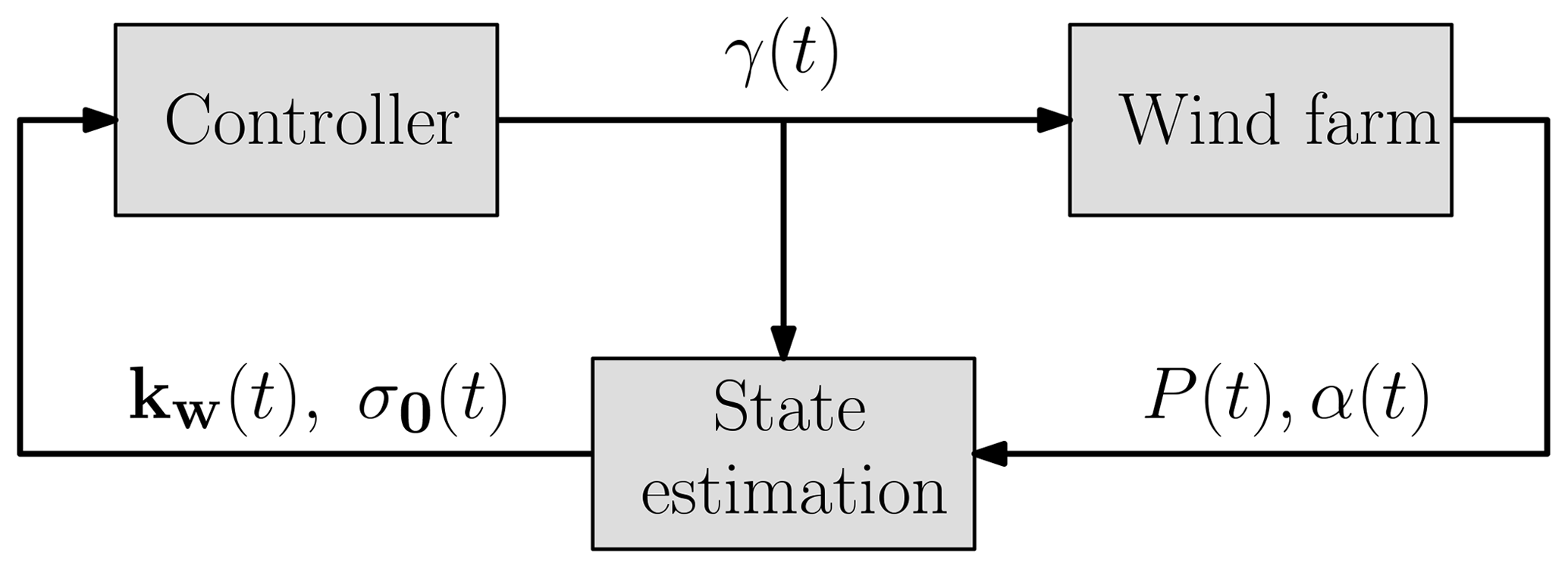
Figure 1 Diagram of the dynamic wake steering control system. The wake model parameters as a function of time are k_w(t) and σ₀(t), and the yaw misalignment angles are given by γ(t). The power production and wind direction are given by P(t) and α(t), respectively. In open-loop control, the model parameters k_w and σ₀ are fixed as a function of time.

2.1 Lifting line wake model

Following the observation of counter-rotating vortex pairs shed by wind turbines operating in yaw misalignment in experiments and LESs (Mikkelsen, 2003; Howland et al., 2016; Bastankhah and Porté-Agel, 2016), Shapiro et al. (2018) developed a wake model for wind turbines in yaw based on Prandtl's lifting line theory. The wake model derived by Shapiro et al. (2018) was reformulated by Howland et al. (2019) to improve computational efficiency and to extract analytic gradients for the purpose of gradient-based optimization. Readers are directed to Shapiro et al. (2018) for the derivation of the initial wake model and to Howland et al. (2019) for the analytic formulation which eliminates the need for domain discretization. In the two dimensional static wake model, the rotor-averaged effective velocity at a downwind wind turbine j is given as

$$\begin{array}{}\text{(1)}& \begin{array}{rl}& u_{\mathrm{e},j}\left(x\right)=u_{\mathrm{\infty }}-\sum _i^{N_{\mathrm{f}}}{\displaystyle \frac{\sqrt{\mathrm{2}\mathit{\pi }}\mathit{\delta }{u}_i\left(x\right)d_{\mathrm{w},i}\left(x\right)D}{\mathrm{16}{\mathit{\sigma }}_{\mathrm{0},i}}}\\ & \left[\mathrm{erf}\left({\displaystyle \frac{y_{\mathrm{T}}+D/\mathrm{2}-y_{\mathrm{c},i}\left(x\right)}{\sqrt{\mathrm{2}}{\mathit{\sigma }}_{\mathrm{0},i}{d}_{\mathrm{w},i}\left(x\right)}}\right)-\text{erf}\left({\displaystyle \frac{y_{\mathrm{T}}-D/\mathrm{2}-y_{\mathrm{c},i}\left(x\right)}{\sqrt{\mathrm{2}}{\mathit{\sigma }}_{\mathrm{0},i}{d}_{\mathrm{w},i}\left(x\right)}}\right)\right],\end{array}\end{array}$$

where u_∞ is the incoming freestream velocity and δu_i and d_w, i are the velocity deficit and the wake diameter as functions of x associated with the upwind turbine i, respectively. The wind turbine rotor diameter is given by D. The downwind turbine lateral centroid is y_T and the lateral wake centroid is y_c, i. The wake model parameters are k_w, the wake spreading coefficient, and σ₀, the proportionality constant for the presumed Gaussian wake. The velocity deficit trailing a single wind turbine is

$$\begin{array}{}\text{(2)}& \mathit{\delta }{u}_i\left(x\right)={\displaystyle \frac{\mathit{\delta }{u}_{\mathrm{0},i}}{d_{\mathrm{w},i}^{\mathrm{2}}\left(x\right)}}{\displaystyle \frac{\mathrm{1}}{\mathrm{2}}}\left[\mathrm{1}+\mathrm{erf}\left({\displaystyle \frac{x}{\sqrt{\mathrm{2}}D/\mathrm{2}}}\right)\right],\end{array}$$

with $\mathit{\delta }{u}_{\mathrm{0},i}=\mathrm{2}{a}_i{u}_{\mathrm{\infty }}$ and axial induction factor $a_i=\mathrm{1}/\mathrm{2}\left(\mathrm{1}-\sqrt{\mathrm{1}-C_{\mathrm{T},i}{\cos }^{\mathrm{2}}\left({\mathit{\gamma }}_i\right)}\right)$. The thrust coefficient is given by C_T, and the yaw misalignment angle is given by γ. The wake model assumes the thrust force in the streamwise direction T∼cos ²(γ) which may not be valid for all wind turbine models (see, e.g., Bastankhah and Porté-Agel, 2016). In the present LES cases, the wind turbine model enforces this thrust scaling (see Sect. 3), and therefore sensitivity analyses on this assumption are left for future work. Positive and negative yaw misalignments are defined as counter-clockwise and clockwise rotations, respectively, when viewed from above. The wake diameter as a function of the streamwise location x is $d_{\mathrm{w},i}\left(x\right)=\mathrm{1}+k_{\mathrm{w},i}\log \left(\mathrm{1}+\exp \left[\mathrm{2}(x/D-\mathrm{1})\right]\right)$. Linear superposition of the individual wakes is assumed in Eq. (1) (Lissaman, 1979).

The wake centerline y_c, i is given by

$$\begin{array}{}\text{(3)}& y_{\mathrm{c},i}=\underset{x_{\mathrm{0},i}}{\overset{x}{\int }}{\displaystyle \frac{-\mathit{\delta }{v}_i\left(x^{\prime }\right)}{u_{\mathrm{\infty }}}}\mathrm{d}{x}^{\prime },\end{array}$$

where the spanwise velocity δv is given similar to Eq. (2) with the initial disturbance given analytically as (Shapiro et al., 2018)

$$\begin{array}{}\text{(4)}& \mathit{\delta }{v}_{\mathrm{0},i}={\displaystyle \frac{\mathrm{1}}{\mathrm{4}}}{C}_{\mathrm{T},i}{u}_{\mathrm{\infty }}{\cos }^{\mathrm{2}}\left({\mathit{\gamma }}_i\right)\sin \left({\mathit{\gamma }}_i\right).\end{array}$$

The wind turbine model power is computed as

$$\begin{array}{}\text{(5)}& {\widehat{P}}_i={\displaystyle \frac{\mathrm{1}}{\mathrm{2}}}\mathit{\rho }{A}_i{C}_{\mathrm{p}}{u}_{\mathrm{e},i}^{\mathrm{3}},\end{array}$$

where A is the wind turbine rotor area and ρ is the density of the surrounding air. The model for the coefficient of power C_p as a function of the yaw misalignment remains an open question. Often, the power loss as a function of the yaw misalignment is assumed to follow $P_{\mathrm{yaw}}\sim P{\cos }^{P_{\mathrm{p}}}\left(\mathit{\gamma }\right)$, where P_p is a known parameter. Following actuator disk theory (Burton et al., 2011), P_p equals 3. However, simulations have shown for the NREL 5 MW turbine that P_p equals 1.88 (Gebraad et al., 2016a). Recent work has shown that P_p differs for freestream and waked turbines (Liew et al., 2020). The value of P_p that results in a satisfactory agreement with experimental data depends on the wind turbine model, ABL shear and veer, and atmospheric stability. In the present study, we will consider P_p an uncertain parameter and perform sensitivity analysis on it. The uncertainties of the wake model parameters k_w and σ₀ are considered by the state estimation in Sect. 2.2. The coefficient of power is modeled as

$$\begin{array}{}\text{(6)}& C_{\mathrm{P},i}=\mathrm{4}\mathit{\eta }{a}_{\mathrm{p},i}{\left(\mathrm{1}-a_{\mathrm{p},i}\right)}^{\mathrm{2}}{\cos }^{P_{\mathrm{p}}}\left({\mathit{\gamma }}_i\right),\end{array}$$

with $a_{\mathrm{p},i}=\frac{\mathrm{1}}{\mathrm{2}}\left(\mathrm{1}-\sqrt{\mathrm{1}-C_{\mathrm{T},i}}\right)$. The parameter η is tuned to match the manufacturer-provided, yaw-aligned C_P look-up table (Gebraad et al., 2016a). The applicability of this model is limited to Region II of the wind turbine power curve which is typically between 4 and 15 m s⁻¹.

2.2 Ensemble Kalman filter state estimation

Engineering wake models rely on parameters which represent physical phenomena such as the wake spreading rate k_w. Gradient optimization-based SCADA data assimilation was used by Howland et al. (2019) to select the model parameters which minimize the model error in producing the site-specific wind farm greedy baseline power production. Howland and Dabiri (2019) subsequently used gradient descent coupled with a genetic algorithm for data assimilation.

Here, we will employ the EnKF (Evensen, 2003) state estimate technique along with the wake model described in Sect. 2.1. The EnKF filter was found to be computationally less expensive than the gradient-based data assimilation used by Howland et al. (2019). The states and dimensions here represent the wake model instantiations and parameters, respectively. In our state estimation case, the dimension space scales linearly with the number of turbines N_t rather than with the $N_{\mathrm{t}}^{\mathrm{2}}$ or $N_{\mathrm{t}}^{\mathrm{3}}$ in a model with a domain discretization (see discussion by Howland et al., 2019). The SCADA power production of each wind turbine is a function of time, denoted P_k, where k is the time step index. The goal is to estimate the wake model parameters given SCADA power production data measurements, $P_k\in {\text{IR}}^{N_{\mathrm{t}}}$, using the ensemble Kalman filter as a rapid gradient-free optimizer (Cleary et al., 2020). This approach follows previous uses of the EnKF for wake model state estimation (Shapiro et al., 2017; Doekemeijer et al., 2017), but the algorithm is reviewed here. The nonlinear wake model, denoted by h, also receives the wind speed and direction from the leading turbine, as well as the yaw misalignment of each turbine in the farm. There are two wake model parameters for each upwind turbine and no parameters for the last turbine downwind. The model parameters with N_t wind turbines at the kth time step are given by

$$\begin{array}{}\text{(7)}& {\mathit{\psi }}_k=\left[k_{\mathrm{w},\mathrm{1}},\mathrm{\dots },k_{\mathrm{w},N_{\mathrm{t}}-\mathrm{1}},{\mathit{\sigma }}_{\mathrm{0},\mathrm{1}},\mathrm{\dots },{\mathit{\sigma }}_{\mathrm{0},N_{\mathrm{t}}-\mathrm{1}}\right].\end{array}$$

The modeling and measurement errors are represented by $\mathit{\chi }={\left[{\mathit{\chi }}_{k_{\mathrm{w}}}^T,{\mathit{\chi }}_{{\mathit{\sigma }}_{\mathrm{0}}}^T\right]}^T\in {\text{IR}}^{\mathrm{2}(N_{\mathrm{t}}-\mathrm{1})}$ and $\mathit{\epsilon }\in {\text{IR}}^{N_{\mathrm{t}}}$, respectively. The modeling errors ${\mathit{\chi }}_{k_{\mathrm{w}}}$ and ${\mathit{\chi }}_{{\mathit{\sigma }}_{\mathrm{0}}}$ are zero mean and have prescribed variances of ${\mathit{\sigma }}_{\mathrm{kw}}^{\mathrm{2}}=\mathrm{0.0009}$ and ${\mathit{\sigma }}_{{\mathit{\sigma }}_{\mathrm{0}}}^{\mathrm{2}}=\mathrm{0.0009}$. The Gaussian random measurement noise ε has zero mean and a prescribed standard deviation of ${\mathit{\sigma }}_{\mathit{\epsilon }}=\mathrm{0.03}\cdot P_{\mathrm{1}}$. The hyperparameter variances were selected based on tuning experiments (see Appendix A). In order to estimate the model parameters, the EnKF uses an ensemble of wake model evaluations. The ensemble is given by

$$\begin{array}{}\text{(8)}& \mathrm{\Psi }=\left[{\mathit{\psi }}^{\left(\mathrm{1}\right)},\mathrm{\dots },{\mathit{\psi }}^{\left(N_{\mathrm{e}}\right)}\right]\in {\text{IR}}^{\mathrm{2}(N_{\mathrm{t}}-\mathrm{1})\times N_{\mathrm{e}}},\end{array}$$

where ⁽ⁱ⁾ denotes the ensemble count and N_e is the total number of ensembles. The power predictions are given by the matrix

$$\begin{array}{}\text{(9)}& \widehat{\mathrm{\Pi }}=\left[{\widehat{\mathit{\pi }}}^{\left(\mathrm{1}\right)},\mathrm{\dots },{\widehat{\mathit{\pi }}}^{\left(N_{\mathrm{e}}\right)}\right]\in {\text{IR}}^{N_{\mathrm{t}}\times N_{\mathrm{e}}}.\end{array}$$

The statistical noise of the power production measurements is given by ε. The Gaussian random noise is added to the SCADA measurements for each ensemble:

$$\begin{array}{}\text{(10)}& {\mathit{\xi }}^{\left(i\right)}=P_{\mathrm{data}}+{\mathit{\epsilon }}^{\left(i\right)}.\end{array}$$

The perturbed power production ensemble matrix is

$$\begin{array}{}\text{(11)}& \mathrm{\Xi }=\left[{\mathit{\xi }}^{\left(\mathrm{1}\right)},\mathrm{\dots },{\mathit{\xi }}^{\left(N_{\mathrm{e}}\right)}\right]\end{array}$$

with the perturbation matrix prescribed by

$$\begin{array}{}\text{(12)}& \mathrm{\Sigma }=\left[{\mathit{\epsilon }}^{\left(\mathrm{1}\right)},\mathrm{\dots },{\mathit{\epsilon }}^{\left(N_{\mathrm{e}}\right)}\right].\end{array}$$

The mean of the ensemble states and modeled power production is given by

$$\begin{array}{}\text{(13)}& {\displaystyle }\stackrel{\mathrm{‾}}{\mathrm{\Psi }}& {\displaystyle }=\mathrm{\Psi }{\mathbf{1}}_{N_{\mathrm{e}}},\text{(14)}& {\displaystyle }\stackrel{\mathrm{‾}}{\widehat{\mathrm{\Pi }}}& {\displaystyle }=\widehat{\mathrm{\Pi }}{\mathbf{1}}_{N_{\mathrm{e}}},\end{array}$$

where ${\mathbf{1}}_{N_{\mathrm{e}}}\in {\text{IR}}^{N_{\mathrm{e}}\times N_{\mathrm{e}}}$ is a full matrix in which all entries are 1∕N_e. The perturbation matrices are

$$\begin{array}{}\text{(15)}& {\displaystyle }{\mathrm{\Psi }}^{\prime }& {\displaystyle }=\mathrm{\Psi }-\stackrel{\mathrm{‾}}{\mathrm{\Psi }},\text{(16)}& {\displaystyle }{\widehat{\mathrm{\Pi }}}^{\prime }& {\displaystyle }=\widehat{\mathrm{\Pi }}-\stackrel{\mathrm{‾}}{\widehat{\mathrm{\Pi }}}.\end{array}$$

The first step in the EnKF process is an intermediate forecast step:

$$\begin{array}{}\text{(17)}& {\displaystyle }{\mathrm{\Psi }}_{k+}& {\displaystyle }=\left[{\mathit{\psi }}_k^{\left(\mathrm{1}\right)}+\mathbf{B}{\mathit{\chi }}_k^{\left(\mathrm{1}\right)},\mathrm{\dots },{\mathit{\psi }}_k^{\left(N_{\mathrm{e}}\right)}+\mathbf{B}{\mathit{\chi }}_k^{\left(N_{\mathrm{e}}\right)}\right],\text{(18)}& {\displaystyle }{\widehat{\mathrm{\Pi }}}_{k+}& {\displaystyle }=\left[h({\mathit{\psi }}_k^{\left(\mathrm{1}\right)}+\mathbf{B}{\mathit{\chi }}_k^{\left(\mathrm{1}\right)}),\mathrm{\dots },h\left({\mathit{\psi }}_k^{\left(N_{\mathrm{e}}\right)}+\mathbf{B}{\mathit{\chi }}_k^{\left(N_{\mathrm{e}}\right)}\right)\right],\end{array}$$

where matrix $\mathbf{B}\in {\text{IR}}^{\mathrm{2}(N_{\mathrm{t}}-\mathrm{1})\times \mathrm{2}(N_{\mathrm{t}}-\mathrm{1})}$ is the identity matrix and h represents the nonlinear wake model described in Sect. 2.1.

The measurement analysis step is given by

$$\begin{array}{}\text{(19)}& \begin{array}{rl}{\mathrm{\Psi }}_{k+\mathrm{1}}=& {\mathrm{\Psi }}_{k+}+{\mathrm{\Psi }}_{k+}^{\prime }\widehat{\mathrm{\Pi }}{{}^{\prime }}_{k+}^T{\left(\widehat{\mathrm{\Pi }}{{}^{\prime }}_{k+}\widehat{\mathrm{\Pi }}{{}^{\prime }}_{k+}^T+{\mathrm{\Sigma }}_{k+\mathrm{1}}{\mathrm{\Sigma }}_{k+\mathrm{1}}^T\right)}^{-\mathrm{1}}\\ & \cdot ({\mathrm{\Xi }}_{k+\mathrm{1}}-{\widehat{\mathrm{\Pi }}}_{k+}).\end{array}\end{array}$$

The final values of k_w and σ₀ for the k+1 time step are given as the columns of ${\stackrel{\mathrm{‾}}{\mathrm{\Psi }}}_{k+\mathrm{1}}$. The EnKF estimation then assumes that the parameters $k_{\mathrm{w},k+\mathrm{1}}$ and ${\mathit{\sigma }}_{\mathrm{0},k+\mathrm{1}}$ will be valid over the succeeding finite time from step k+1 until step k+2. A schematic of the EnKF methodology is shown in Fig. 2.

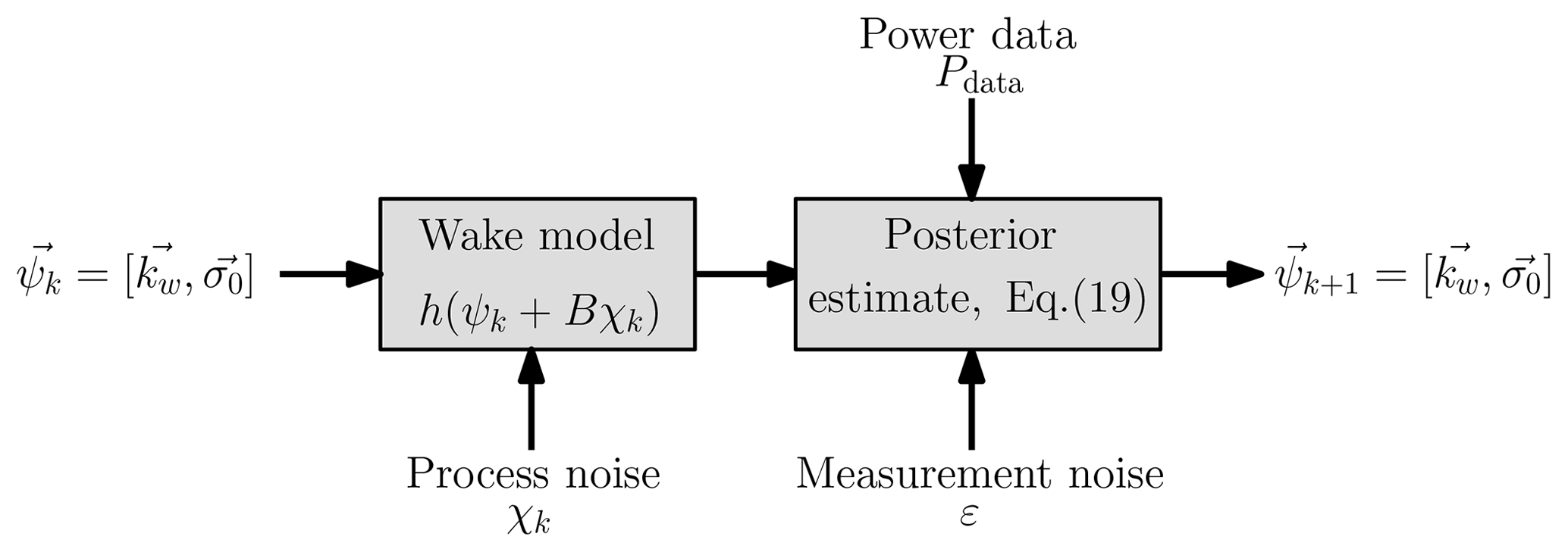
Figure 2 Schematic of the ensemble Kalman filter parameter estimation methodology. The wake model predicts the power production given the wake model parameters ψ_k from time step k and the modeled process noise χ. The power data from the LES are augmented with modeled measurement noise ε. The wake model predictions, h(ψ_k+Bχ_k), process and measurement noise, and power data are leveraged to compute the parameters in the k+1 time step ψ_k+1 using the measurement analysis step (Eq. 19).

The EnKF is a Kalman filter method which uses the Monte Carlo sampling of model parameters according to a prescribed Gaussian function to represent the covariance matrix of the probability density function (PDF) of the state vector Ψ. The likelihood of the data is represented using observations Ξ and prescribed perturbations Σ. Using the prior PDF of the state (k) and data likelihood, the posterior state (k+1) is estimated using Bayes's rule (Eq. 19).

2.3 Optimal yaw misalignment optimization

The optimal yaw misalignment angles depend on the wind speed, direction, turbulence intensity, and other key ABL conditions. Within a given condition bin, the number of potential yaw misalignment angle combinations grows exponentially with the number of wind turbines. As such, brute force optimization methods are not sufficient for the selection of the optimal yaw misalignment strategy. Previous studies have considered genetic algorithms (Gebraad et al., 2016a), discrete gradient-based optimization (Gebraad et al., 2017), and analytic gradient-based optimization (Howland et al., 2019). Using a gradient-based Adam optimization (Kingma and Ba, 2014), the gradient update is given by

$$\begin{array}{}\text{(20)}& {\mathit{\gamma }}^{t+\mathrm{1}}={\mathit{\gamma }}^t-\mathit{\alpha }{\displaystyle \frac{m_t}{\sqrt{v_t}}},\end{array}$$

where $m^t={\mathit{\beta }}_{\mathrm{1}}{m}^{t-\mathrm{1}}+(\mathrm{1}-{\mathit{\beta }}_{\mathrm{1}})\frac{\partial \sum \widehat{P}}{\partial \mathit{\gamma }}$ and $v^t={\mathit{\beta }}_{\mathrm{2}}{v}^{t-\mathrm{1}}+(\mathrm{1}-{\mathit{\beta }}_{\mathrm{2}})(\frac{\partial \sum \widehat{P}}{\partial \mathit{\gamma }}{)}^{\mathrm{2}}$. The hyperparameters are set to the commonly used values of β₁=0.9 and β₂=0.999, respectively (Kingma and Ba, 2014). The analytic gradients computed by Howland et al. (2019) are used for the gradient-based wind farm power optimization.

3 Large eddy simulation setup

Large eddy simulations are performed using the open-source pseudo-spectral code PadéOps¹. The solver uses sixth order compact finite differencing in the vertical direction (Nagarajan et al., 2003) and Fourier collocation in the horizontal directions. Temporal integration uses a fourth-order-strong, stability-preserving Runge–Kutta variant (Gottlieb et al., 2011). The LES code has previously been utilized for high Reynolds number ABL flows (Howland et al., 2020a; Ghaisas et al., 2020) and is described in detail by Ghate and Lele (2017). The ABL is modeled as an incompressible, high Reynolds number limit (Re→∞) flow with the filtered, nondimensional momentum equations given by

$$\begin{array}{}\text{(21)}& {\displaystyle }\begin{array}{rl}{\displaystyle \frac{\partial u_i}{\partial t}}+u_j{\displaystyle \frac{\partial u_i}{\partial x_j}}=& -{\displaystyle \frac{\partial p}{\partial x_i}}-{\displaystyle \frac{\partial {\mathit{\tau }}_{ij}}{\partial x_j}}+f_i+{\displaystyle \frac{{\mathit{\delta }}_{i\mathrm{3}}}{{\mathit{Fr}}^{\mathrm{2}}}}\left(\mathit{\theta }-{\mathit{\theta }}_{\mathrm{0}}\right)\\ & -{\displaystyle \frac{\mathrm{2}}{\mathit{Ro}}}{\mathit{\epsilon }}_{ijk}{\mathrm{\Omega }}_j{u}_k-{\displaystyle \frac{\partial P^{\mathrm{G}}}{\partial x_i}},\end{array}\text{(22)}& {\displaystyle \frac{\partial u_i}{\partial x_i}}=\mathrm{0},\end{array}$$

where u_i is the velocity in the x_i direction, p is the nondimensional pressure, and P^G is the nondimensional geostrophic pressure. The subfilter-scale stress tensor is given by τ_ij, and the sigma model is employed (Nicoud et al., 2011). The turbulent Prandtl number used in the subfilter-scale model is Pr=0.4 (Ghate and Lele, 2017). Surface stress and heat flux are computed using a local wall model based on Monin–Obukhov similarity theory with appropriate treatment based on the state of stratification (Basu et al., 2008). The wind turbine forcing is represented by f_i, and a nonrotating actuator disk model is used (Calaf et al., 2010). The actuator disk thrust force acts parallel to the rotor normal vector. The incident velocity is projected into the rotor disk plane, and therefore the dependence of thrust on the yaw misalignment γ in uniform inflow conditions would be cos ²(γ), although it may deviate from this in sheared and veered inflow conditions. While the actuator disk model is lower fidelity than the actuator line methods, it captures the far wake (far wake is approximately x∕D≳3; see, e.g., Bastankhah and Porté-Agel, 2017) accurately for both aligned (Martínez-Tossas et al., 2015) and yaw misalignment wind turbines (Lin and Porté-Agel, 2019). Since the goal of the present study is controller synthesis and sensitivity experiments, more computationally expensive actuator line simulations are left for future work given the large volume of simulations that are run.

Earth's rotational vector is given by $\mathrm{\Omega }=\left[\mathrm{0},\cos \left(\mathit{\varphi }\right),\sin \left(\mathit{\varphi }\right)\right]$, where ϕ is the latitude. The traditional approximation, which neglects the horizontal component of Earth's rotation (Leibovich and Lele, 1985; Howland et al., 2018), is not enforced. Therefore, Earth's full rotational vector is included resulting in wind farm dynamics which are sensitive to the direction of the geostrophic wind (Howland et al., 2020b). For simplicity, all simulations are performed with west to east geostrophic wind. The Coriolis terms are parameterized by the Rossby number $\mathit{Ro}=G/\mathit{\omega }L$, where G is the geostrophic wind speed magnitude, ω is Earth's angular velocity, and L is the relevant length scale of the problem. All wind speeds used in this study will be normalized by the geostrophic wind speed magnitude. The nondimensional potential temperature is given by θ. The buoyancy term is parameterized by the Froude number $\mathit{Fr}=G/\sqrt{gL}$, where g is the gravitational acceleration. The equation for the transport of the filtered nondimensional potential temperature is given by

$$\begin{array}{}\text{(23)}& {\displaystyle \frac{\partial \mathit{\theta }}{\partial t}}+u_j{\displaystyle \frac{\partial \mathit{\theta }}{\partial x_j}}=-{\displaystyle \frac{\partial q_j^{\mathrm{SGS}}}{\partial x_j}},\end{array}$$

where $q_j^{\mathrm{SGS}}$ is the subgrid scale (SGS) heat flux.

The wind is forced by prescribing the geostrophic approximation where the geostrophic pressure gradient drives the mean flow (Hoskins, 1975). The geostrophic pressure balance in the stable free atmosphere is given by

$$\begin{array}{}\text{(24)}& {\displaystyle \frac{\partial P^{\mathrm{G}}}{\partial x_i}}=-{\displaystyle \frac{\mathrm{2}}{\mathit{Ro}}}{\mathit{\epsilon }}_{ijk}{\mathrm{\Omega }}_j{G}_k,\end{array}$$

with G_k representing the geostrophic velocity vector.

The simulations utilize a fringe region to force the inflow to a desired profile (Nordström et al., 1999). In the conventionally neutral ABL cases, the concurrent precursor method is applied, wherein a separate LES of the ABL is run without wind turbine models and the fringe region is used to force the primary simulation outflow to match the concurrent precursor simulation outflow (see, e.g., Munters et al., 2016; Howland et al., 2020a).

There is an initial startup transience following the domain initialization. Detailed comments on the initialization for the conventionally neutral case are given by Howland et al. (2020b). The simulation cases are run until statistical quasi-stationarity is reached. The conventionally neutral case is statistically quasi-stationary due to inertial oscillations (see Allaerts and Meyers, 2015, for a detailed discussion on the conventionally neutral ABL statistical quasi-stationarity). Upon convergence, the wake steering control strategy is initiated.

The control is initialized with a greedy baseline yaw alignment which is fixed for n_T time steps. After n_T simulation steps, with the time-averaged power production for each wind turbine measured over the previous n_T−T_a time steps and with the advection timescale given by T_a, the EnKF estimation and optimal yaw calculations are performed (Fig. 1). The time lag associated with the advection timescale of the wind farm is estimated by invoking Taylor's hypothesis (see Appendix C for a brief discussion). The yaw angles are then implemented and held fixed for n_T time steps, and the cycle repeats. The wind speed, wind direction, and power production are averaged in time over the window. The state estimation and yaw misalignment update steps are performed concurrently with a period of n_T simulation steps. In general, these two processes can be decoupled, although this was not investigated in the present study. Typical utility-scale wind turbines have a yaw rate of approximately 0.5^∘ s⁻¹ (Kim and Dalhoff, 2014). For the largest yaw misalignment change in one control update step in this study of approximately 30^∘, when the wake steering control is initialized, the yawing action is completed in approximately 1 min, which is significantly less than the advection timescale in the flow. Therefore, the yaw rate will not influence the results presented in this study.

In order to compare the power production of the yaw misalignment control strategy with the baseline greedy control, a separate LES case is run for each experiment with yaw-aligned control. The two simulations are initialized from identical domain realizations, and the computational time step Δt is fixed between the two cases. Therefore, without the influence of variable turbine operation, the flow within and around the turbine array is identical to machine precision between the two yaw-aligned and yaw-misaligned cases². Since this study will consider the conventionally neutral ABL which contains turbulence and inertial oscillations, this separate simulation must be used instead of a comparison with the power production of the first yaw control update step (see Appendix B).

Figure 3 Conventionally neutral six wind turbine finite wind farm simulation setup. The geostrophic wind direction is west to east, and the x axis is aligned with the geostrophic wind direction. The mean wind direction at hub height is ${\tan }^{-\mathrm{1}}(\stackrel{\mathrm{‾}}{v}/\stackrel{\mathrm{‾}}{u})\approx \mathrm{16}$^∘, but it is not known a priori in the simulation and varies as a function of time. The wind turbine array is offset from alignment in the x direction by 18^∘. The initial boundary layer height δ₀ is 700 m and does not change significantly during runtime (see Fig. 4). Fringe functions are applied in the x and y directions to establish a finite wind farm simulation.

The wind turbines have a rotor diameter of 126 m and a hub height of 100 m. The thrust coefficient is C_T=0.75. The initial boundary layer height is 700 m. The domain size is $\mathrm{12}\mathrm{km}\times \mathrm{6}\mathrm{km}\times \mathrm{2.4}\mathrm{km}$ in the x, y, and z directions, respectively, with z representing the wall-normal coordinate. The number of grid points is $\mathrm{480}\times \mathrm{240}\times \mathrm{192}$ with a grid spacing of $\mathrm{25}\mathrm{m}\times \mathrm{25}\mathrm{m}\times \mathrm{12.5}\mathrm{m}$. The grid spacing is uniform, the mesh size is similar to previous studies (Allaerts and Meyers, 2015), and a grid convergence study was performed by Howland et al. (2020b) for the conventionally neutral ABL. Six model wind turbines are incorporated in the domain, and the layout within the computational domain is shown in Fig. 3. The Rossby number based on the wind turbine diameter is 544, and the Froude number is 0.14. The vertical profiles of velocity, potential temperature, and streamwise turbulence intensity for the precursor simulation for two domain snapshots are shown in Fig. 4.

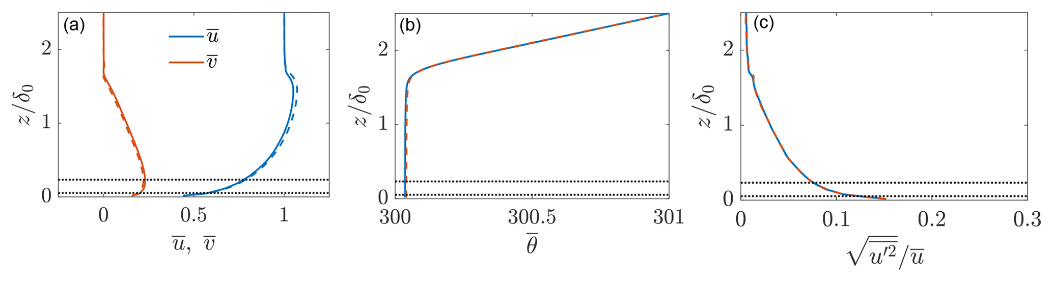
Figure 4 Horizontally averaged, concurrent precursor conventionally neutral ABL LES (a) velocity, (b) potential temperature in Kelvin, and (c) turbulence intensity. Horizontally averaged profiles from two different time instances are shown with solid (early) and dashed (late) lines, qualitatively demonstrating that the flow is statistically quasi-stationary (see further discussion by Howland et al., 2020a). Dashed-dotted lines show the extents of the turbine rotor area.

4 Dynamic wake steering conventionally neutral atmospheric boundary layer LES

In this section, we will utilize the closed-loop wake steering controller in the conventionally neutral ABL. While the conventionally neutral ABL is statistically quasi-stationary, the optimal yaw misalignment angles will vary as a function of time due to turbulence, large-scale streamwise structures (Önder and Meyers, 2018), and inertial oscillations. A suite of LES cases is run to test the influence of the controller architecture design, state estimation design, P_p estimate (Eq. 6), and the wind farm layout on the power production increases over the greedy baseline operation as a result of wake steering control. Each sensitivity study represents a new LES case which is run using the concurrent precursor methodology described in Sect. 3.

All quasi-steady conventionally neutral ABL simulations have a yaw controller update of n_T=1000 time steps which are approximately equal to τ=3000 seconds or 50 min. The advection timescale from the first to the last wind turbine in the array is approximately 9 min, and the time lag is taken as 2 times the approximate advection timescale based on Taylor's hypothesis. Therefore, each update contains approximately 30 min of statistical averaging or about 600 time steps. The long time averaging window was selected since the flow is statistically quasi-stationary and to ensure temporal averages with reduced noise. In transitioning ABL environments, the time averaging window should likely be reduced (Kanev, 2020). The baseline case (Case NA) has yaw-aligned control. The yaw alignment for each wind turbine in the array in the greedy baseline controller is updated according to the same timescale τ based on the mean wind direction measured locally by each wind turbine. The nacelle position for the yaw-misaligned turbines is based on the wind direction measurement at each local turbine, as well as the controller estimated optimal yaw misalignment angles, i.e., $n_{\mathit{\alpha }}=\mathit{\alpha }+\mathit{\gamma }$, where n_α is the nacelle position and α is the wind direction incident to the wind turbine. Therefore, the LES accounts for the effects of secondary steering.

This section is organized as follows: Sect. 4.1 examines the sensitivity of the wind turbine array power production to the wake steering controller design. Section 4.2 tests the sensitivity to the state estimation methodology. The sensitivity of the wake steering control to the estimate of P_p is discussed in Sect. 4.3. The accuracy of the wake model power predictions is discussed in Sect. 4.4. Appendix E characterizes the influence of the wind farm alignment on the wake steering power production increase.

Table 1 The conventionally neutral finite wind farm wake steering cases. The mean power production increase with respect to yaw-aligned operation is calculated over approximately 24 h of physical wind farm operation. Case NA is the yaw-aligned wind farm operation. Case NL approximates open-loop lookup-table-based control. Cases beginning with ND are dynamic, closed-loop control cases with various control architectures as denoted in the table. The wake model estimate for P_p is ${\widehat{P}}_{\mathrm{p}}$.

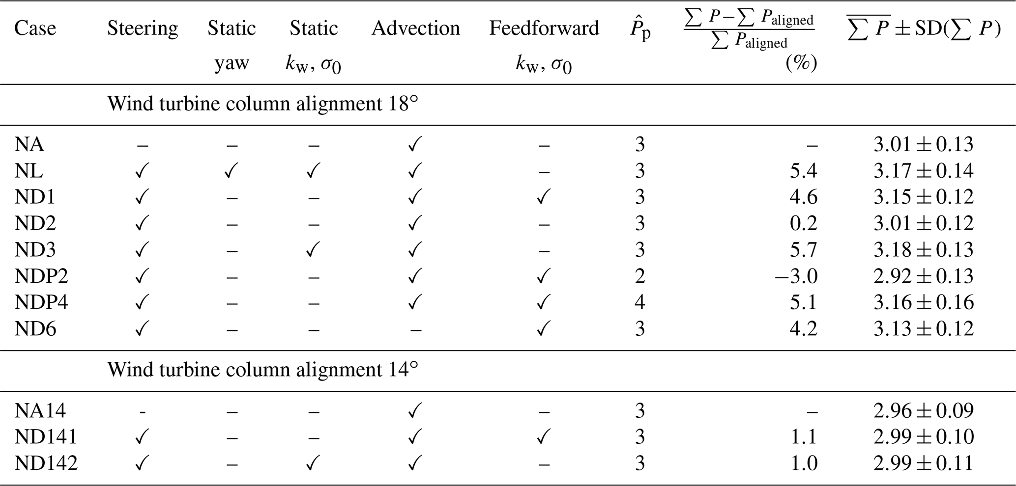
The conventionally neutral ABL wake steering LES cases and results are summarized in Table 1. Baseline yaw-aligned wind turbine operation is given by Case NA, in which the yaw alignment is updated at the same temporal frequency as the dynamic yaw control is updated to ensure quantitative comparisons as a function of time. Case NL approximates open-loop lookup table operation, in which the yaw misalignment is prescribed as a function of the incident wind speed and direction rather than dynamically adapting to the local inflow conditions. Cases ND1, ND2, and ND3 use dynamic wake steering control with varying parameter estimation techniques. In Case ND1 the wake model parameters are optimized continuously based on a fixed parameter initialization. Cases ND1 and NL are discussed in detail in Sect. 4.1. In Case ND2, the model parameters are optimized continuously in time based on an initialization using the previous time step optimal parameters, and finally Case ND3 fixes the wake model parameters after the estimation in the first control update step. The influence of the state estimation techniques is discussed in detail in Sect. 4.2. Cases NDP2 and NDP4 modify the wake model estimate for P_p and are described in more detail in Sect. 4.3. Finally, Case ND6 is the same as Case ND1 except it sets the advection time T_a equal to 0. Cases NA14, ND141, and ND142 modify the wind farm alignment to 14^∘ with respect to the horizontal axis and are described in more detail in Appendix E.

Figure 5 Time-averaged sum of the six-turbine-array power production for the conventionally neutral ABL LES cases described in Table 1. The error bars denote 1 standard deviation in the power production. The power production is normalized by the leading turbine P₁ in baseline control conditions. The statistical significance of the wake steering power production difference with respect to the baseline control Case NA is indicated by the colors. The statistical significance is characterized by a one-sided two-sample Kolmogorov–Smirnov test at a 5 % significance level. Case NA is blue, and Case ND2 does not have a statistically significantly greater power production than Case NA. Green cases have statistically significantly (p<0.05) more power than Case NA. Red cases have statistically significantly (p<0.05) less power than Case NA.

The statistical significance of the array power productions for the various wake steering cases with respect to the baseline control Case NA are shown in Fig. 5. The statistical significance is characterized with one-sided two-sample Kolmogorov–Smirnov tests for the given case with respect to the baseline control Case NA at a 5 % significance level. The Kolmogorov–Smirnov test was selected since it does not enforce a normal distribution assumption on the data. Cases NL, ND1, ND3, NDP4, and ND6 produce significantly more power than the baseline control Case NA. Case NDP2 produces significantly less power than baseline control, and Case ND2 is not significantly different from Case NA. None of cases NL, ND1, ND3, NDP4, and ND6 are significantly different from each other. The power production for each turbine for each wake steering case is shown in Fig. 6.

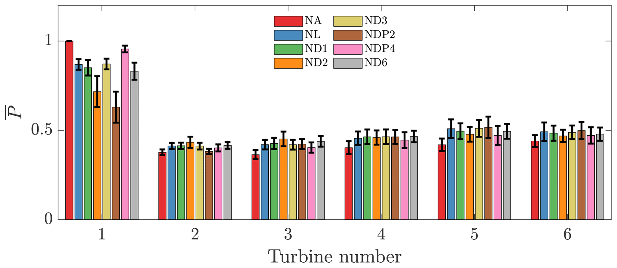
Figure 6 Time-averaged power production for each turbine in each wake steering case. The error bars denote 1 standard deviation in the power production. The power production is normalized by the leading turbine P₁ in baseline control conditions.

4.1 Comparison between dynamic and quasi-static wake steering approaches

The dynamic wake steering controller described in Fig. 1 is compared to the lookup table static control in this section. Since the flow is statistically quasi-stationary, the mean wind speed and direction at hub height do not change significantly as a function of time. Therefore, during simulation, the flow remains at wind conditions which would be associated with one wind speed and direction bin in the tabulated lookup table wake steering control. The lookup table control is approximated by fixing the yaw misalignment angles as a function of time after the initial optimal angles are computed during the first yaw controller update (Case NL). Numerical experiments (not shown for brevity) demonstrated that modifying the control update step from which the lookup yaw misalignment values were computed did not have a statistically significant influence on the results for Case NL. The dynamic yaw controller is represented by Case ND1. The time-averaged wind speed at the wind turbine hub height for cases NA and NL are shown in Fig. 7. As a result of the positive yaw misalignment strategy in Case NL (Fig. 7b), the individual and collective array wakes are deflected in the clockwise direction compared to the aligned configuration of Case NA (Fig. 7a).

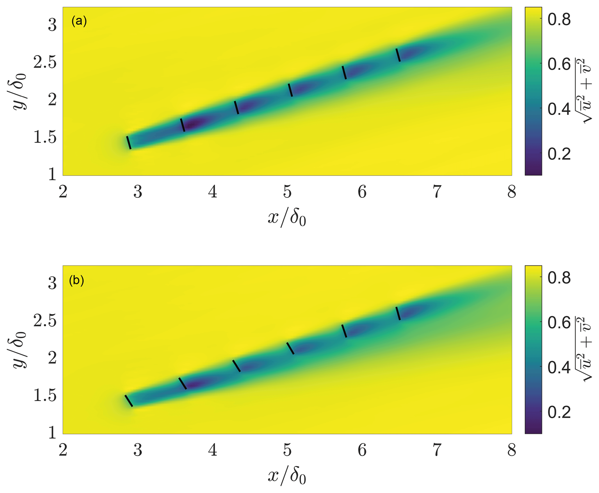
Figure 7 Time-averaged wind speed $\sqrt{{\stackrel{\mathrm{‾}}{u}}^{\mathrm{2}}+{\stackrel{\mathrm{‾}}{v}}^{\mathrm{2}}}$ at the wind turbine hub height of z=100 m for (a) baseline yaw-aligned control Case NA and (b) wake steering control Case NL. The wind turbines are shown with black lines. The yaw misalignment values for Case NL are shown in Fig. 8.

The yaw misalignment angles as a function of the yaw controller updates for cases NL and ND1 are shown in Fig. 8. The yaw angles in this study are defined as the misalignment with respect to the local inflow direction incident on the particular turbine in the array. While the lifting line model does not explicitly incorporate the effects of secondary steering for which model development is ongoing (see, e.g., King et al., 2020), the model selects yaw misalignment angles which are large for the first turbine and generally decrease further into the wind farm, which is consistent with the optimal values found by recent wind tunnel experiments (Bastankhah and Porté-Agel, 2019). Since the flow is statistically quasi-stationary, the dynamic algorithm yaw misalignment angles do not change significantly as a function of time. There are a few yaw misalignment changes on the order of 10^∘ during one yaw update. The time-averaged power productions as a function of the yaw controller updates for the two cases are shown in Fig. 9. The qualitative trends in power production are similar between the two cases. Quantitatively, the lookup table static yaw misalignment Case NL increased the power production 5.4 % with respect to the baseline greedy control, while the dynamic yaw Case ND1 increased the power by 4.6 %.

The quantitative influence of wake steering is a function of the layout and ABL conditions. As the focus of the present study is assessing the sensitivity of wake steering to controller architecture, model parameters, and wind farm layout, measures of the statistical significance of the results are useful. However, the statistical significance of the results (e.g., whether Case NL significantly outperformed Case ND1) does not indicate, necessarily, that lookup table control is better than the dynamic controller used in Case ND1 for all wake steering applications but rather that it was better for the specific ABL setup and computational time window of the experiment. The statistical significance of the power production increase with respect to the baseline control Case NA is shown in Fig. 5. Cases NL and ND1 have significantly higher power than Case NA, but the power in Case NL is not significantly higher than in Case ND1.

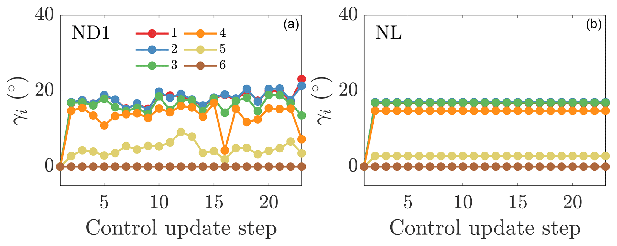
Figure 8 Wind farm yaw misalignment angles γ_i for each turbine for (a) online control using the initial parameters to initialize the next state (ND1) and (b) the lookup table control (NL).

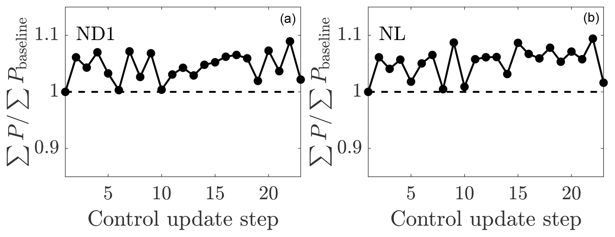
Figure 9 Time-averaged wind farm power production as a function of the control update steps for (a) online control using the initial parameters to initialize the next state (ND1) and (b) the lookup table control (NL). The wind farm power is normalized by the power production of the aligned wind farm case.

The relationship between the wake model power prediction and the measured LES power production is shown for the two cases in Fig. 10. The wake model overpredicts the power production in yaw misalignment more for the dynamic yaw control than the lookup table control. After the first time step, the wake model no longer has any state information for the LES power production with the greedy baseline control since the previous state had yaw misalignment. When the wake model overpredicts the expected LES power, the wake model parameters are updated to a state which expects larger wake loss effects in baseline control; therefore, the yaw misalignment angles are increased at the next time step. The yaw misalignment angles for the leading turbine oscillate around the lookup table optimal forecast which was based on the calibration with power data from the greedy baseline control alone (Fig. 8). The dynamic yaw increased power slightly less than the static yaw misalignment case but not significantly less. However, eliminating the need to tabulate historical data and the complexity of implementing a lookup-table-based controller could be beneficial in a practical controller setting. Further, the conventionally neutral boundary layer does not occur often in practice (Hess, 2004). Therefore, in a practical setting, the wind direction and speed at hub height will not be fixed for multiple hours as in this test problem.

In Case ND6, the power productions are time averaged over the full n_T window without considering the advection timescale in the controller design. The power production increase over the greedy control is 4.2 % in this case, which is less than the 4.6 % increase when considering the advection time lag (Case ND1), although this difference is not significant. The dynamics of the closed-loop controller over long experimental horizons are tested in a 50 control update simulation in Appendix D.

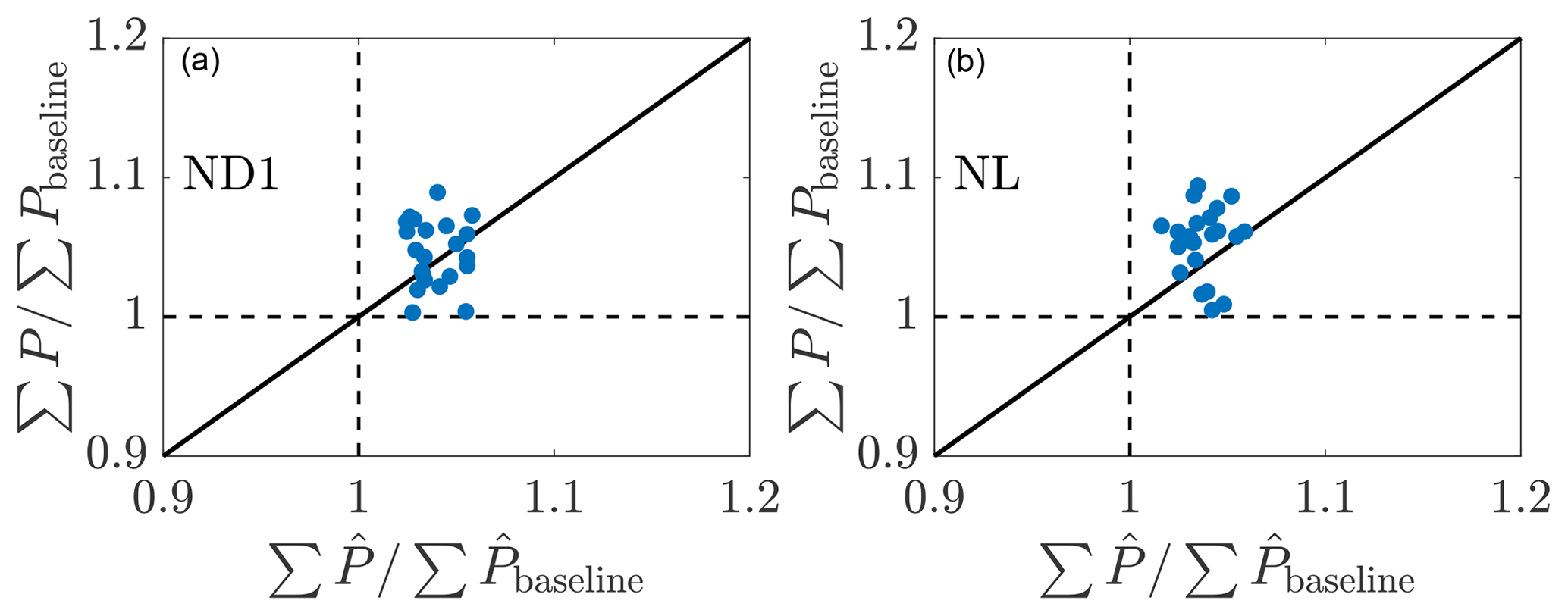
Figure 10 Relationship between the LES wind farm power production compared to the wake model wind farm power production prediction for (a) online control using the initial parameters to initialize the next state (ND1) and (b) the lookup table control (NL). The wind farm power is normalized by the power production of the aligned wind farm case. The LES power production is given by P, and the wake model prediction is given by $\widehat{P}$.

4.2 Influence of the state estimation

The influence of the state estimation methodology is tested in this section. Within the conventionally neutral ABL, three experiments focused on the state estimation initialization are run. The initial model parameters in the EnKF estimation are held fixed at k_w=0.1 and σ₀=0.25 in Case ND1. In Case ND2, the optimal EnKF estimated parameters from the previous time step are used to initialize the state estimation of the current time step. Finally, Case ND3 fixes the model parameters after the first time step. Case ND3 differs from Case NL from Section 4.1 since the optimal yaw misalignment angles may vary as a function of time, while the model parameters do not.

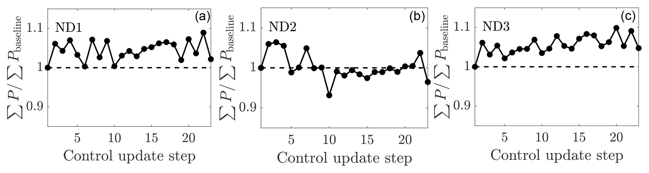
Figure 11 Time-averaged wind farm power production as a function of the control update steps for (a) online control using the initial parameters to initialize the next state (ND1), (b) online control using the previous optimal parameters to initialize the next state (ND2), and (c) the static state estimation control (ND3). The wind farm power is normalized by the power production of the aligned wind farm case.

The power productions as a function of the yaw controller update for the three cases are shown in Fig. 11. Case ND2 has significantly less power production than cases ND1 and ND3. The time-averaged power production increases with respect to the baseline; the greedy control is 4.6 %, 0.2 %, and 5.7 % for cases ND1, ND2, and ND3, respectively. The power productions in cases ND1 and ND3 are significantly higher than in Case NA, while in Case ND2 it is not. Further, cases ND1 and ND3 are significantly better than ND2, but Case ND3 is not significantly better than ND1. In the EnKF methodology described in Sect. 2.2, the update step to the wake parameters is limited by the imposed parameter variance (${\mathit{\sigma }}_{k_{\mathrm{w}}}$ and ${\mathit{\sigma }}_{{\mathit{\sigma }}_{\mathrm{0}}}$). Therefore, the initialization of the EnKF with fixed parameters limits the perturbation of the estimated parameters as a function of time, whereas the initialization with the previous optimal parameters allows k_w and σ₀ to vary more significantly over time. The EnKF estimated k_w and σ₀ for the three cases are shown in Figs. 12 and 13, respectively. While the proportionality constant σ₀ of the presumed Gaussian wake does not have a clear trend for Case ND2, the estimated wake spreading rate k_w is clearly decreasing for all wind turbines as a function of time. For Case ND1, the estimated model parameters do not have a clear trend and remain approximately constant as a function of time. As the estimated wake spreading rate is decreased, the wake model predicts worsening wake interactions and lower array power production given the greedy baseline control. As a result, the model-predicted optimal yaw misalignment angles increase as a function of time for Case ND2, as shown in Fig. 14a. While cases ND1 and ND3 predict the optimal yaw misalignment for the most upwind turbine to be approximately 20^∘ and decreasing γ moving downwind, Case ND2 increases the yaw misalignment for the upwind turbine to as high as 30^∘.

Figure 12 Wake spreading coefficient for each turbine in the wind farm for (a) online control using the initial parameters to initialize the next state (ND1), (b) online control using the previous optimal parameters to initialize the next state (ND2), and (c) the static state estimation control (ND3).

Figure 13 Proportionality constant for the presumed Gaussian wake for each turbine in the wind farm for (a) online control using the initial parameters to initialize the next state (ND1), (b) online control using the previous optimal parameters to initialize the next state (ND2), and (c) the static state estimation control (ND3).

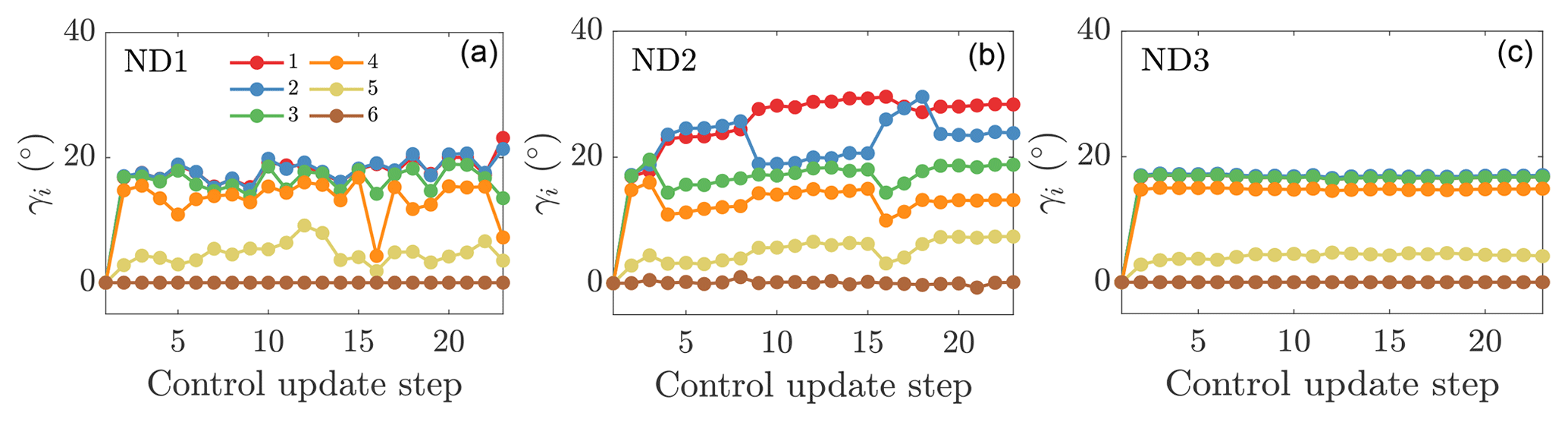
Figure 14 Yaw misalignment angles for each turbine in the wind farm for (a) online control using the initial parameters to initialize the next state (ND1), (b) online control using the previous optimal parameters to initialize the next state (ND2), and (c) the static state estimation control (ND3).

The relationship between the model-predicted and LES-measured power production for the three cases is shown in Fig. 15. Case ND2 has an increased occurrence of wake model overprediction of the power production, while Case ND3 has an increased occurrence of wake model underprediction. Case ND1 has an approximately equal occurrence of underprediction and overprediction. The efficacy of the state estimation is shown in Fig. 16. Both cases ND1 and ND2 are able to estimate the power production for the downwind turbine in the baseline greedy operation (the first time step) and with yaw misalignment. Since Case ND3 uses static state estimation, there are some discrepancies between the LES power production and the lifting line model (Fig. 16c). The power production for the most upwind turbine is modeled accurately using P_p=3, although the LES power production is generally slightly lower, indicating P_p>3 for this actuator disk model (ADM) and ABL state.

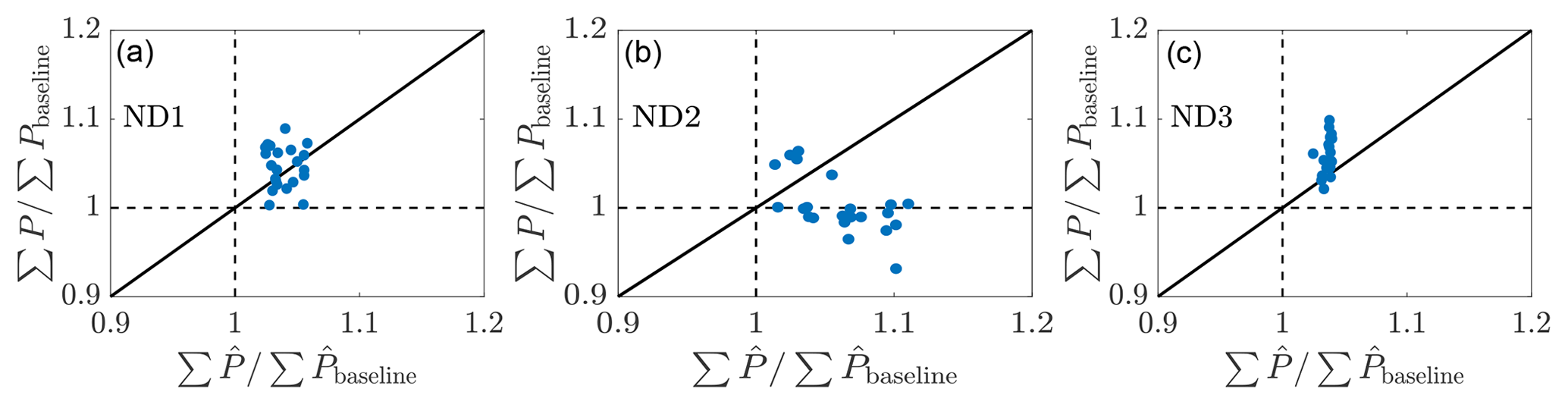
Figure 15 Relationship between the LES wind farm power production compared to the wake model wind farm power production prediction for (a) online control using the initial parameters to initialize the next state (ND1), (b) online control using the previous optimal parameters to initialize the next state (ND2), and (c) the static state estimation control (ND3). The LES power production is given by P, and the wake model prediction is given by $\widehat{P}$.

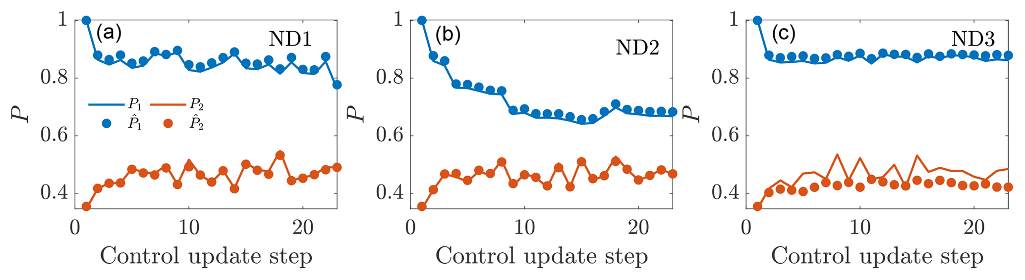
Figure 16 Time-averaged power production for the first and second wind turbines in the wind farm as a function of the control update steps for (a) online control using the initial parameters to initialize the next state (ND1), (b) online control using the previous optimal parameters to initialize the next state (ND2), and (c) the static state estimation control (ND3). The LES power production is given by P, and the wake model state estimation is given by $\widehat{P}$.

The most successful dynamic control framework utilized in the conventionally neutral ABL is the static state estimation methodology (Case ND3), although the differences between cases ND1 (parameter estimation from standard initialization), ND3 (static parameters after first control step), and NL (static yaw angles after first control step) are not significant. While the optimal yaw misalignment angles change slightly as a function of time (Fig. 14), the wake model parameters are fixed. Since the flow is statistically quasi-stationary, the wake model parameters should not change significantly as a function of time. However, the wake model parameters may have a functional dependence on γ, the yaw misalignment for the upwind turbines. This potential dependence of k_w and σ₀ on yaw misalignment was not incorporated explicitly in the present modeling framework, although it is incorporated implicitly through the state estimation, and it is recommended for investigation in future work.

The static state estimation with dynamic yaw controller is able to outperform the lookup table control (Table 1). This indicates that while the wake model parameters are fixed, the optimal yaw misalignment angles differ even with changes to the mean wind direction less than 1^∘. As such, the lookup-table-based yaw misalignment strategy is unlikely to be optimal in a general setting since it relies on wind speed and direction bins of arbitrary size. Instead, in a lookup table approach, the wake model parameters could be tabulated instead of the optimal yaw misalignment angles. Optimal yaw misalignments can be calculated dynamically on the fly using the computationally efficient model described in Sect. 2.1, or a mid-fidelity model (e.g., WFSim; Boersma et al., 2018) could be used to compute discrete yaw angles in wind condition bins, and the continuous optimal yaw function could be approximated using interpolating functions or a neural network, for example.

4.3 Influence of the estimate of P_p in the wake model

The wind turbine power production as a function of the yaw misalignment in the wake model is given by Eq. (6). The parameter P_p is uncertain. Following actuator disk theory, P_p approximately equals 3, although experiments typically show P_p≤2 for wind turbines and wind turbine models with rotation (e.g., Medici, 2005). With the ADM used presently, P_p=3 should be an accurate approximation but will be imperfect since actuator disk theory applies only to spatially uniform, steady flow. Since P_p is wind-turbine-specific and likely site-specific, in a wake steering application, the precise value of P_p is generally unknown a priori. In this section, we will model P_p as ${\widehat{P}}_{\mathrm{p}}=\mathrm{2}$ (NDP2) and ${\widehat{P}}_{\mathrm{p}}=\mathrm{4}$ (NDP4) using the same control architecture as Case ND1, in which ${\widehat{P}}_{\mathrm{p}}$ denotes the wake model estimate for P_p. ${\widehat{P}}_{\mathrm{p}}=\mathrm{2}$ will lead to an underestimate of the power production loss due to yaw misalignment, and ${\widehat{P}}_{\mathrm{p}}=\mathrm{4}$ will lead to an overestimate. Given that the value of P_p is turbine-specific, the influence of the P_p uncertainty described in this section should be considered relative to the true value of P_p=3, and the conclusions apply with respect to the scaled values of ${\widehat{P}}_{\mathrm{p}}/P_{\mathrm{p}}$. For a different turbine model with P_p=2, for example, similar values of ${\widehat{P}}_{\mathrm{p}}/P_{\mathrm{p}}$ would yield qualitatively similar results.

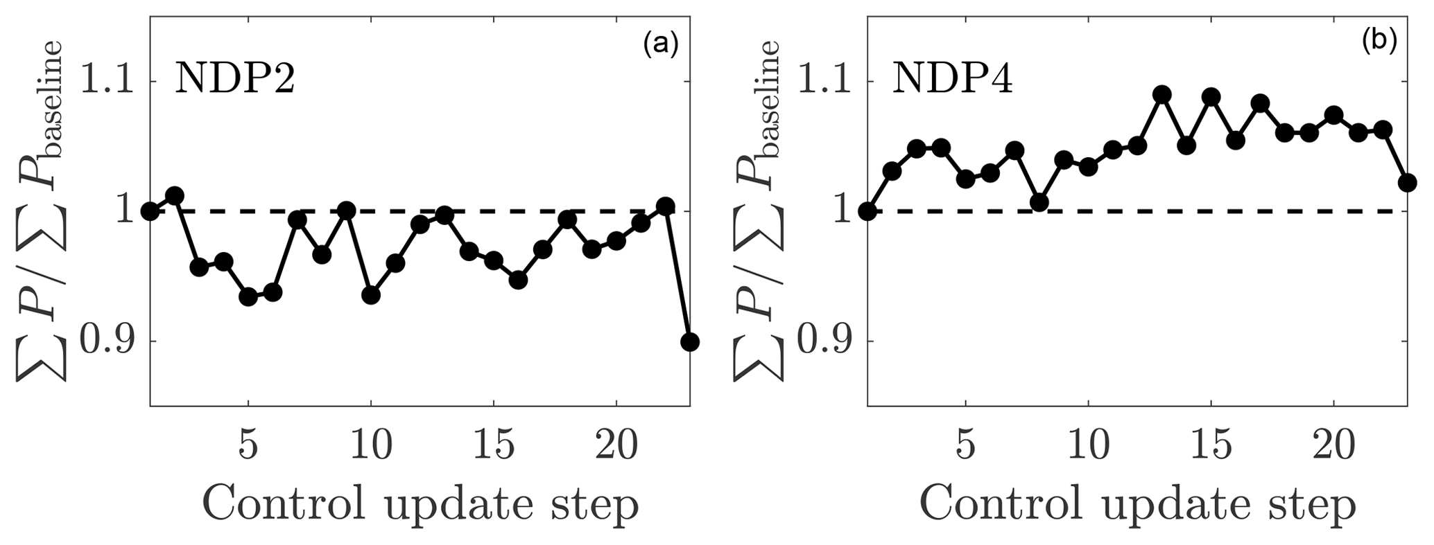
Figure 17 Time-averaged wind farm power production as a function of the control update step for online control using the initial parameters to initialize the next state and (a) ${\widehat{P}}_{\mathrm{p}}=\mathrm{2}$ (NDP2) and (b) ${\widehat{P}}_{\mathrm{p}}=\mathrm{4}$ (NDP4). The wind farm power is normalized by the power production of the aligned wind farm case.

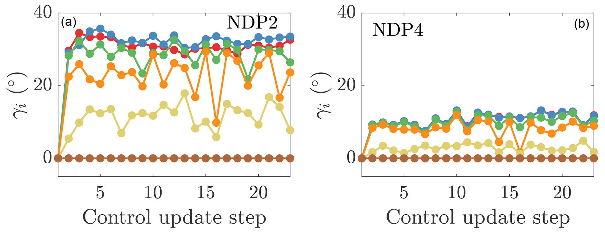
Figure 18 Yaw misalignment angles for each turbine in the wind farm for online control using the initial parameters to initialize the next state and (a) ${\widehat{P}}_{\mathrm{p}}=\mathrm{2}$ (NDP2) and (b) ${\widehat{P}}_{\mathrm{p}}=\mathrm{4}$ (NDP4).

The power productions as a function of the yaw update steps for cases NDP2 and NDP4 are shown in Fig. 17. Case NDP2 with ${\widehat{P}}_{\mathrm{p}}=\mathrm{2}$ has 3.0 % less power production than the baseline greedy operation, while Case NDP4 with ${\widehat{P}}_{\mathrm{p}}=\mathrm{4}$ has 5.1 % more power than the baseline control. Case ND1 and NDP4 have significantly higher power production than NDP2. With ${\widehat{P}}_{\mathrm{p}}=\mathrm{2}$, the model prediction for the optimal yaw misalignment angles is high, with the first three upwind turbines misaligning by almost γ=40^∘ (Fig. 18a). With ${\widehat{P}}_{\mathrm{p}}=\mathrm{4}$, the penalty for yaw misalignment is significant, and no turbine misaligns more than γ=20^∘ (Fig. 18b). For the present conventionally neutral ABL and ADM implemented, the value is $\mathrm{3}<P_{\mathrm{p}}<\mathrm{4}$ for the leading upwind turbine. The success of Case NDP4 with ${\widehat{P}}_{\mathrm{p}}=\mathrm{4}$ suggests that small yaw misalignments can still increase the wind farm power production significantly with respect to the baseline greedy control.

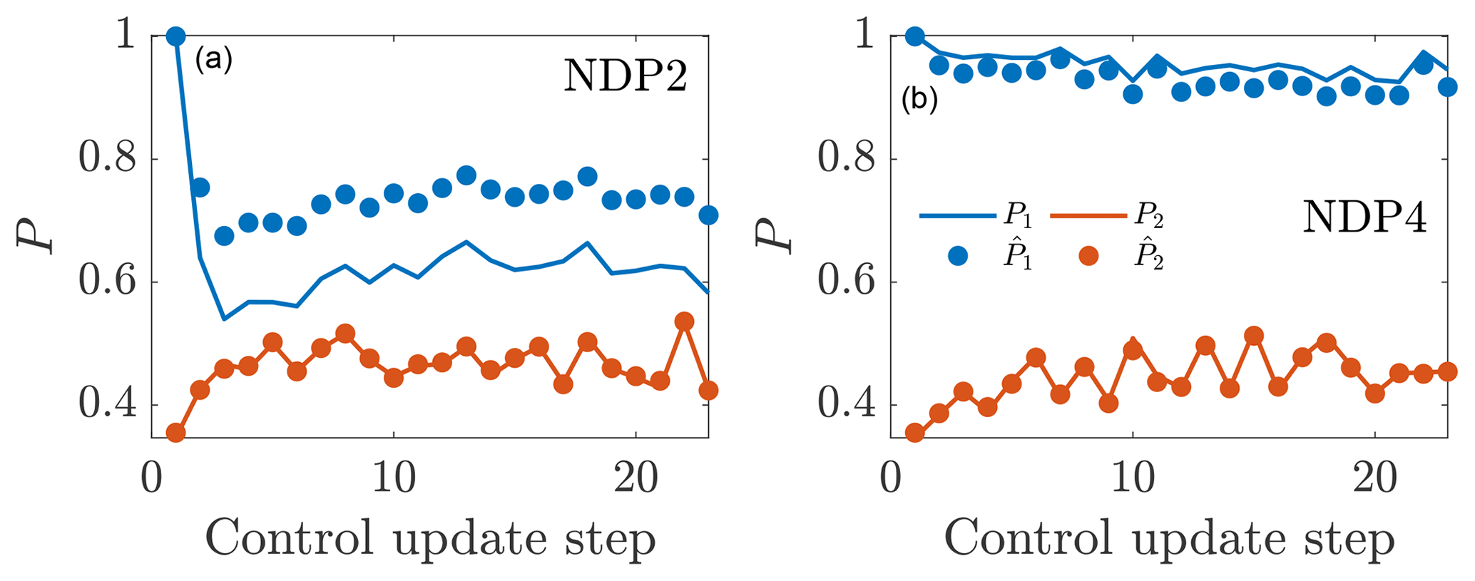
Figure 19 Time-averaged power production for the first and second wind turbines in the wind farm as a function of the control update steps for online control using the initial parameters to initialize the next state and (a) ${\widehat{P}}_{\mathrm{p}}=\mathrm{2}$ (NDP2) and (b) ${\widehat{P}}_{\mathrm{p}}=\mathrm{4}$ (NDP4). The LES power production is given by P, and the wake model state estimation is given by $\widehat{P}$.

The LES power productions and EnKF estimated power productions as a function of the yaw control updates are shown for the two ${\widehat{P}}_{\mathrm{p}}$ cases in Fig. 19. For Case ND4, the upwind turbine power production is significantly overpredicted. The EnKF does not estimate the state for the most upwind turbine since there are no wake model parameters which influence its production. The power production for the second wind turbine is accurately estimated even with ${\widehat{P}}_{\mathrm{p}}=\mathrm{2}$. This shows that the state estimation with a two-parameter model is potentially over-parameterized where the EnKF is compensating for the incorrect P_p model by altering k_w and σ₀ unphysically, although the consequence of this effect in the accuracy of the power predictions will be discussed in Sect. 4.4. The power productions and EnKF estimations for the first two wind turbines for Case ND5 show that ${\widehat{P}}_{\mathrm{p}}=\mathrm{4}$ is a more accurate estimate than ${\widehat{P}}_{\mathrm{p}}=\mathrm{2}$. Again, the downwind turbine power is estimated accurately with the incorrect value of ${\widehat{P}}_{\mathrm{p}}$.

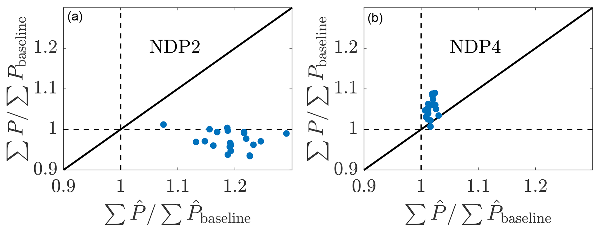
Figure 20 Relationship between the LES wind farm power production compared to the wake model wind farm power production prediction for online control using the initial parameters to initialize the next state and (a) ${\widehat{P}}_{\mathrm{p}}=\mathrm{2}$ (NDP2) and (b) ${\widehat{P}}_{\mathrm{p}}=\mathrm{4}$ (NDP4). The LES power production is given by P, and the wake model prediction is given by $\widehat{P}$.

The comparison between the wake model power predictions against the LES power production is shown in Fig. 20. With ${\widehat{P}}_{\mathrm{p}}=\mathrm{2}$ (Fig. 20a), the wake model significantly overpredicts the power production of the wind turbine array with expected power increases over the baseline of 25 % but a power decrease with respect to the baseline realized. On the other hand, with ${\widehat{P}}_{\mathrm{p}}=\mathrm{4}$ (Fig. 20b), the wake model underpredicts the power production of the wind turbine array for nearly all control update steps. Comparing Figs. 15b and 20b, it is clear that, in this simulation, the lifting line model prediction of downwind turbine power is less conservative as a function of increasing γ. Therefore, the model is likely slightly overestimating the true optimal yaw misalignment angle magnitudes when P_p equals 3.

Overall, the sensitivity analysis on P_p suggests that given a model application where P_p is unknown, a conservative estimation should be taken. With the present data-driven dynamic controller, underestimating P_p leads to the wake model estimating a state which would lead to high wake losses with the baseline greedy control. There is no pathway for the state estimation to discern the discrepancy between an incorrect P_p model or, for example, changing atmospheric conditions which are giving rise to worsening wake losses given the baseline control. Future work should focus on methodologies to robustly estimate P_p from SCADA data. Further, the potential deviation of the wind turbine thrust from cos ²(γ) (Bastankhah and Porté-Agel, 2016) should be investigated in a similar manner as P_p in future work.

4.4 Accuracy of wake model predictions

The accuracy of the wake model power predictions are assessed in this section by comparing the LES power measurements to the wake model power predictions from the previous time step. As detailed in Sect. 3, the simulation is initialized with greedy yaw alignment which is held fixed for n_T time steps (control update 1), after which yaw misalignment angles are implemented for n_T steps (control update 2). The yaw angles are subsequently updated dynamically every n_T simulation steps. At control update 1, the previous n_T steps of yaw-aligned operation are used to compute P_baseline, the time-averaged power production for each wind turbine. P_baseline is used to estimate k_w and σ₀ using the EnKF such that $\left|P_{\mathrm{baseline}}-{\widehat{P}}_{\mathrm{baseline}}\right|$ is minimized. With the estimated model parameters, the optimal yaw misalignment angles are computed for each wind turbine. Using the estimated k_w and σ₀ and the optimal yaw angles computed at control update 1, ${\widehat{P}}_{\mathrm{yaw}}$ is predicted, which is attempting to represent P_yaw, the average power production over the n_T steps following control update 1. The computation of P_yaw is completed at control update 2 and can be compared directly to ${\widehat{P}}_{\mathrm{yaw}}$ to validate the predictive capabilities of the lifting line model and the estimated model parameters. In short, ${\widehat{P}}_{\mathrm{baseline}}$ represents P_baseline, and it is an estimation or fit because the model had knowledge of P_baseline. ${\widehat{P}}_{\mathrm{yaw}}$ is a prediction since the model had no knowledge of P_yaw. The LES-measured and wake-model-estimated and wake-model-predicted power productions are shown in Fig. 21 for ${\widehat{P}}_{\mathrm{p}}=\mathrm{2}$, 3, and 4.

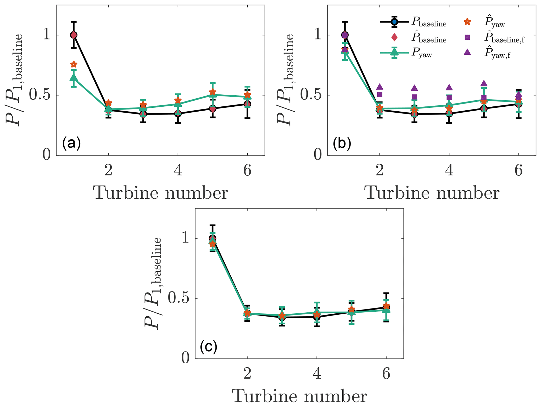
Figure 21 Wind turbine power production from LES P and wake model $\widehat{P}$. P_{1, baseline} is the LES power production for the leading upwind turbine from control update step 1 where the wind farm is operated with the greedy baseline control. ${\widehat{P}}_{\mathrm{baseline}}$ is the wake model fit to P_baseline using EnKF estimation. P_yaw is the LES power production for control update step 2 with yaw misalignment incorporated. ${\widehat{P}}_{\mathrm{yaw}}$ is the wake model prediction of P_yaw using k_w and σ₀ fit based on control update step 1 and with the optimal yaw misalignment angles which were implemented by control update step 1. The wake model estimate for P_p, given by ${\widehat{P}}_{\mathrm{p}}$, is (a) ${\widehat{P}}_{\mathrm{p}}=\mathrm{2}$, (b) ${\widehat{P}}_{\mathrm{p}}=\mathrm{3}$, and (c) ${\widehat{P}}_{\mathrm{p}}=\mathrm{4}$. The error bars represent 1 standard deviation in the power data as a function of time. The subscript “f” denotes power predictions from the FLORIS wake model (Annoni et al., 2018) with the Gaussian wake model (Bastankhah and Porté-Agel, 2014) and model parameters prescribed by Niayifar and Porté-Agel (2016).

The mean absolute error for the lifting line model power estimation was 0.0037 for all three cases since ${\widehat{P}}_{\mathrm{p}}$ does not affect the fitting with yaw-aligned control enforced. The mean absolute errors for the lifting line model power predictions were 0.044, 0.015, and 0.018, given as a fraction of P_{1, baseline}, for ${\widehat{P}}_{\mathrm{p}}=\mathrm{2}$, 3, and 4, respectively. The mean absolute errors as a function of the control update steps for the three simulations are shown in Fig. 22. The averages over the control update steps of the mean absolute errors for the three cases are 0.05, 0.029, and 0.036 for ${\widehat{P}}_{\mathrm{p}}=\mathrm{2}$, 3, and 4, respectively. Qualitatively, ${\widehat{P}}_{\mathrm{p}}=\mathrm{3}$ and 4 result in predictions which are accurate and within 1 standard deviation of the mean. ${\widehat{P}}_{\mathrm{p}}=\mathrm{2}$ results in more inaccurate predictions, with elevated inaccuracy for the leading upwind turbine. Overall, these results, in tandem with the field experiment results of Howland et al. (2019), suggest that the lifting line model (Shapiro et al., 2018) provides accurate predictions of the power production of wind farms within yaw misalignment given the data-driven calibration to yaw-aligned operational data.

The baseline and yaw-misaligned power predictions using the FLORIS wake model package (Annoni et al., 2018) are also shown in Fig. 21. The FLORIS model implementation uses the Gaussian wake model (Bastankhah and Porté-Agel, 2014) with the wake spreading rate k^* approximated using the empirical LES fit between k^* and the turbulence intensity given by Niayifar and Porté-Agel (2016). Since the Gaussian wake model parameters are not calibrated to the site-specific LES of this wind farm, the inaccuracy in representing P_baseline is expected according to the typical fidelity of engineering wake models (Stevens and Meneveau, 2017). The mean absolute error for the power production prediction in yaw misalignment averaged over the six wind turbines in the array is 0.02P_{1, baseline} and 0.11P_{1, baseline} for the lifting line model with data assimilation and for the Gaussian model with an empirical wake spreading rate as a function of turbulence intensity, respectively. P_{1, baseline} is the power production of the leading upwind turbine in the greedy control. The EnKF data assimilation has reduced the error in the prediction of the power production in yaw misalignment by an order of magnitude compared to a priori prescribed empirical model parameters. Since the greedy wake losses in FLORIS differ from the LES power production, FLORIS will also predict different yaw misalignment angles in its model-based optimization. For greenfield applications before wind farm construction, SCADA data are not available, and data assimilation methods cannot be used, necessitating empirical methods such as those suggested by Niayifar and Porté-Agel (2016). For operational wind farm control optimization, site-specific data assimilation increases the accuracy of the model predictions (Fig. 21b).

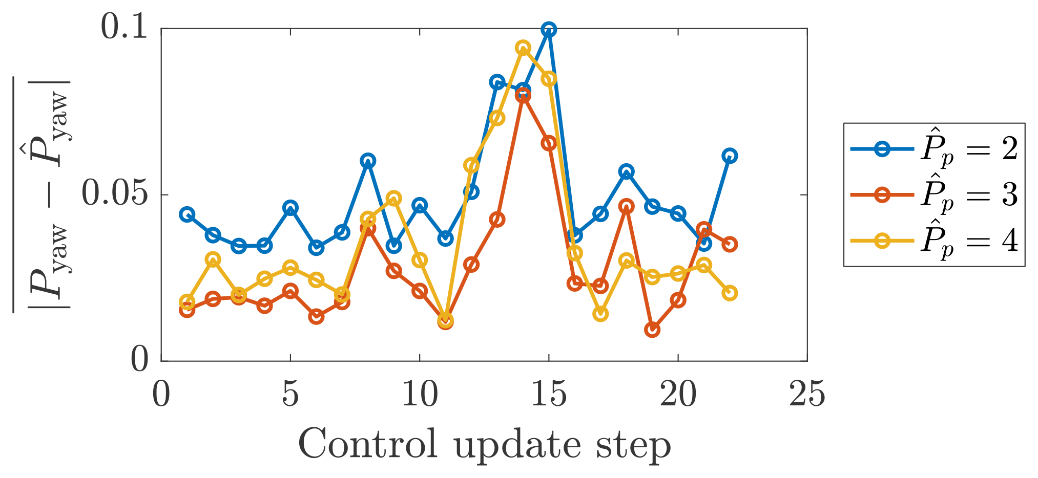
Figure 22 The mean absolute errors for the lifting line model predictions as a function of the control update step for the conventionally neutral ABL with ${\widehat{P}}_{\mathrm{p}}=\mathrm{2}$, 3, and 4.

5 Conclusions

A suite of large eddy simulations has been performed to characterize the performance of a dynamic, closed-loop wake steering wind farm control strategy. The controller was designed for the application of real-time utility-scale wind farm control based on only SCADA data without requiring a lidar on site. The analytic gradient ascent optimal yaw selection allows for real-time dynamic wind farm control. The main technical contribution of this paper is the development of a closed-loop wake steering methodology for application in transient ABL flows which does not rely on an open-loop offline yaw misalignment lookup table calculation.

Within the statistically quasi-stationary, conventionally neutral ABL, the optimal yaw misalignment angles do not change significantly with time. Within this simplified ABL environment, wake steering control with fixed lookup table yaw misalignment values, dynamic yaw values with continuous state estimation, and dynamic yaw values with fixed state estimation all yielded significantly more power than the baseline control, although the differences between the three control architectures were not significant. The highest power production occurred with a wake steering strategy in which the model parameters were fixed and the state estimation was not performed for every control update step but the yaw misalignment angles were updated according to the local wind conditions. This result suggests that in a lookup table wake steering approach, the wake model parameters should be tabulated and the yaw angles should be calculated on the fly given exact local wind conditions rather than direct optimal yaw misalignment angle tabulation.

The importance of the model for individual wind turbine power production degradation as a function of the yaw misalignment angle, and in particular P_p, was demonstrated when ${\widehat{P}}_{\mathrm{p}}=\mathrm{3}$ or 4 leads to an increase in power production with respect to the greedy operation, while ${\widehat{P}}_{\mathrm{p}}=\mathrm{2}$ leads to a loss in power with the true P_p=3. Since P_p depends on the wind turbine model and ABL characteristics, this should be investigated in future work.

The wake model does not capture all relevant physical phenomena present in this flow (see specific assumptions in wake model derivation in Sect. 2.1), but the power production is fit accurately as a function of time with the two parameter model. While this success may suggest that the site- and time-specific parameter estimations may correct for physics which are unresolved in the model, with ${\widehat{P}}_{\mathrm{p}}=P_{\mathrm{p}}=\mathrm{3}$, the wake model makes accurate forecasts of the power production over a future time horizon given the yaw misalignment strategy that was implemented. In this study, the wake model forecast has low predictive error when the wake model parameter modifications are constrained in the EnKF estimation as in Case ND1 rather than unconstrained as a function of time, as in Case ND2, which results in high predictive error and diminished wake steering performance. The forecast accuracy gives confidence to the data-driven EnKF parameter estimation and lifting line wake model for the application of wake steering control. The combined lifting line model and EnKF estimation has an order of magnitude reduced predictive error than the Gaussian wake model with an empirical wake spreading rate in this conventionally neutral ABL simulation. The magnitude of model parameter modifications as a function of time is implicitly constrained in this study by the hyperparameters of the EnKF estimation algorithm. Future work should investigate the predictive capabilities of combined data-driven and wake model approaches with explicit constraints on the model parameters.

While the conventionally neutral ABL cases were not designed to model a specific wind farm and to be compared with field data, this LES test bed paradigm is useful for the rapid prototyping of optimal wind farm control architectures. The main purpose of this study was predominantly to establish the dynamic wake steering framework and perform sensitivity analyses on the controller architecture rather than the ABL or LES setup. The uncertainties and sensitivities in this study associated with the wall model, subfilter-scale model, wind turbine model, and ABL characteristics such as boundary layer inversion height were not investigated in detail and are left for future work. More reliable and generalizable estimates for P_p (Liew et al., 2020), or generally C_p as a function of γ, should be investigated. Future work should also investigate the influence of latitude and geostrophic wind direction on wake steering control performance (Howland et al., 2020b). Finally, the controller should be tested using other LES codes and in field experiments to assess the generalization of the results. Part 2 of this study will implement the dynamic optimal controller in transient ABL conditions such as the stable ABL and the diurnal cycle.

Appendix A: EnKF test model problem

The state estimation EnKF algorithm and implementation are tested using a six wind turbine model wind farm with artificial data. Six 1.8 MW Vestas V80 wind turbines are modeled with an incoming wind speed of u_∞=7.5 m s⁻¹. The turbines are spaced 6 rotor diameters (D) apart in the streamwise direction and are directly aligned in the spanwise direction as shown in Fig. A1a. The test problem was used for hyperparameter selection to achieve estimations of the artificial power production with low mean absolute error. The parameters selected for the EnKF algorithm are ${\mathit{\sigma }}_{k_{\mathrm{w}}}=\mathrm{0.001}$, ${\mathit{\sigma }}_{{\mathit{\sigma }}_{\mathrm{0}}}=\mathrm{0.001}$, and σ_P=0.1. The initial wake model parameters were selected as k_w=0.1 and σ₀=0.35 for each wind turbine in the array. The model is run with a specified, artificial mean power production profile with Gaussian random noise superposed. The model is run over 1000 model time step iterations with N_e=100. The initial and final model calibrations are shown in Fig. A1b and c. The EnKF combined with the lifting line model is able to fit the artificial wind farm data with sufficient accuracy for two different power production profiles.

Figure A1 (a) Model problem setup. (b, c) The EnKF model fits for the model problem with two prescribed, artificial mean power profiles and Gaussian random noise. (d) Model parameters shown with solid (b) and dashed (c) lines. The wake model parameters for the last turbine downwind are not shown since they do not impact the state estimation accuracy.

As shown in Fig. A1b and c, the EnKF state estimation combined with the lifting line model is able to reproduce the power production for the artificial data to high accuracy. While the ability for a two parameter analytic wake model to capture arbitrarily generated power production profiles should be investigated in future studies, this data-driven framework is validated in the LES test cases in a comparison between model power predictions and LES power measurements (Sect. 4.4) in which the state estimation significantly reduces the power predictions compared to standard empirical wake model approaches.

Appendix B: Influence of local atmospheric conditions on wind turbine array power production

The quantification of the influence of new control methods on the wind farm power production is challenging in an experimental setting. In a computational environment, simulations with identical initial conditions and fixed time stepping schemes can be used to quantify the influence of the operational modifications in a controlled experiment. In a field experiment environment, since wind conditions are constantly changing and are not repeatable due to the nature of atmospheric flows, this quantification is more challenging. Complex terrain and differences in the manufacturing and operation of turbines in standard control leads to substantial discrepancies in the instantaneous power production of freestream turbines at wind farms. Therefore, comparing yaw-misaligned columns of turbines to yaw-aligned columns leads to uncertainty in the analysis. Further, conditional averages based on wind speed, direction, turbulence intensity, and atmospheric conditions may not sufficiently capture the potential physical mechanisms which influence power production. To quantify this impact in the present simulations, the power productions as a function of the control update steps can be compared to the first control update step in the statistically quasi-stationary, conventionally neutral ABL flow. Inertial oscillations, turbulence, and sampling error will cause discrepancies between the first and subsequent control update steps even with the yaw-aligned control strategy held fixed in the statistically quasi-stationary flow. The average power production compared to the first yaw control update step is 4.3 % and 9.0 % higher for the yaw-aligned (Case NA) and dynamic closed-loop (Case ND1) controls, respectively. The increase observed in Case NA indicates that the simulation had not completely converged to the statistically quasi-stationary state upon control initialization, although this does not affect the qualitative conclusions of Sect. 4. The true increase in power production due to wake steering in Case ND1 compared to Case NA is 4.6 % over the same simulation temporal window. These results highlight the need to develop robust statistical methods to analyze the impact of changing wind farm control strategies compared to the baseline.

Figure B1 Time-averaged power production as a function of time normalized by the time-averaged power production of the first control update step for the yaw-aligned greedy control. (a) Yaw-aligned greedy control (Case NA) and (b) closed-loop dynamic control (Case ND1).

Appendix C: Approximate advection timescale

Upon the yaw misalignment of an upwind turbine, there is a time lag associated with the advection timescale of the flow for the control decision to influence a downwind turbine. While the advection time depends on the length scale of the turbulent eddy (Del Álamo and Jiménez, 2009; Yang and Howland, 2018; Howland and Yang, 2018), the mean flow advection approximately follows the mean wind speed in wind farms (Taylor, 1938; Lukassen et al., 2018). The number of simulation time steps associated with the approximate advection time between the first and last turbines is computed as

$$T={\displaystyle \frac{\mathrm{\Delta }{s}_x}{{\stackrel{\mathrm{‾}}{u}}_{\mathrm{hub}}\mathrm{\Delta }t}},$$

where Δs_x is the distance between the first and last turbine in the streamwise direction, ${\stackrel{\mathrm{‾}}{u}}_{\mathrm{hub}}$ is the mean streamwise velocity at the wind turbine model hub height, and Δt is the simulation time step. In the computation of wind farm statistics for the utilization of static wake models, the advection timescale is accounted for by initializing the time-averaging, two advection timescales T_a=2T after the yaw misalignments for the wind turbine array have been updated. To account for errors associated with the simple advection model, the time lag is taken as double the advection timescale, T_a=2T, although this advection timescale did not have a statistically significant influence on the results, as shown in Table 1 and Fig. 5.

Appendix D: Extended conventionally neutral simulation

The conventionally neutral ABL Case ND1 is run for 50 control update steps, and the results are shown in Fig. D1. The controller does not become unstable as a function of time, and the magnitude of yaw misalignment angles are approximately constant.

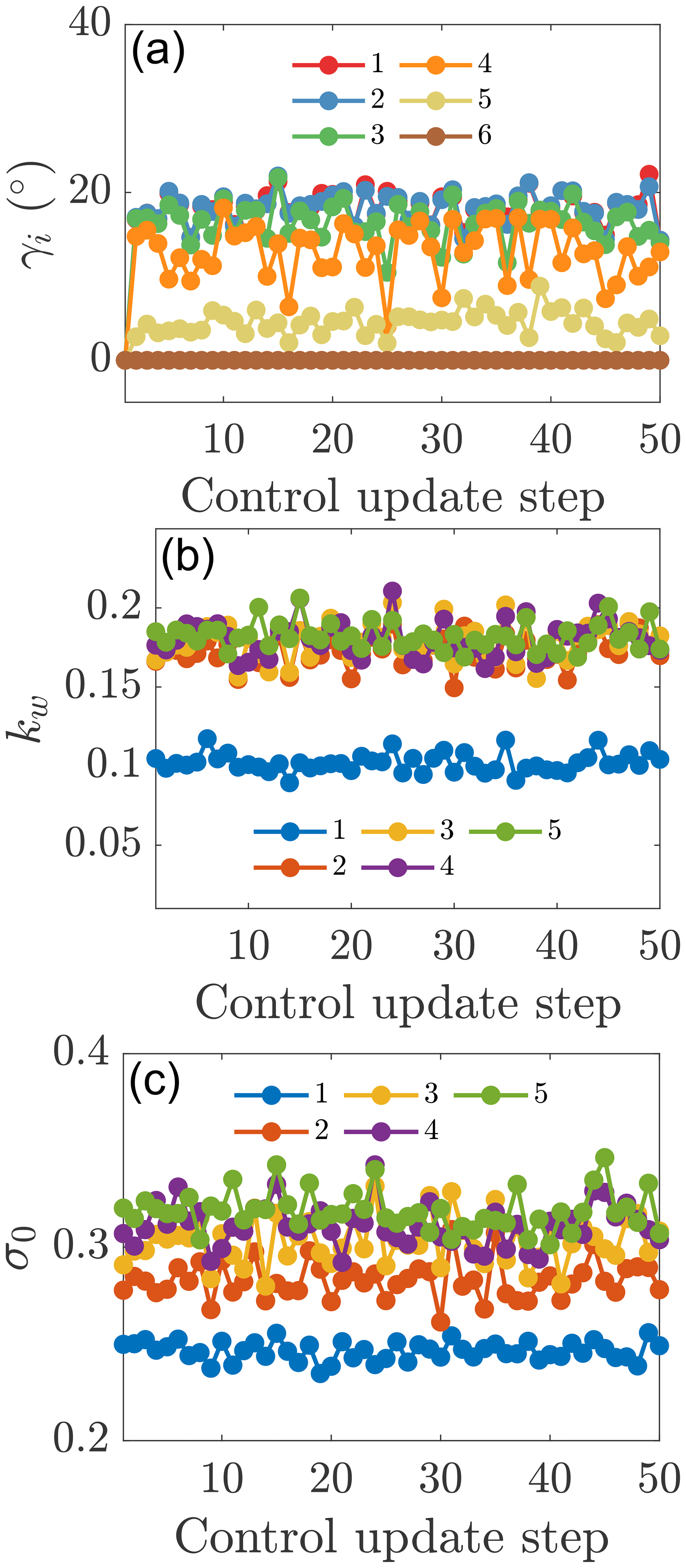
Figure D1 Wind farm (a) yaw misalignment angles, (b) k_w, and (c) σ₀ as a function of the control update steps for the extended ND1 case.

Appendix E: Influence of the wind farm alignment in the conventionally neutral ABL

The wake losses and potential for wake steering to increase wind turbine array power production depend on the wind turbine layout (see, e.g., experiments by Bossuyt et al., 2017). In the previous section, the six wind turbines were aligned at an angle of 18^∘ from the horizontal (Fig. 3). The mean wind direction at hub height is approximately 15–16^∘ in this conventionally neutral ABL. In this section, the wind turbine column alignment is changed to 14^∘ from the horizontal, and the array is embedded within the same conventionally neutral ABL. As a result of this array alignment, the optimal yaw misalignment angles will change from positive (counter-clockwise rotation viewed from above) to negative (clockwise). It should be noted that this sensitivity analysis is not a controlled experiment to test the benefit of yawing in opposite directions since asymmetries exist in the conventionally neutral ABL as a result of the veer angle, and the magnitude of partial waking is not held fixed between the two layouts.

For the wind turbine array aligned at 14^∘, the dynamic wake steering controller is tested with dynamic (ND141) and static state (ND142) estimations. With a wind farm alignment along 14^∘ and the mean wind direction at hub height of approximately 15–16^∘, the optimal yaw misalignment angles are negative (clockwise viewed from above). The yaw misalignment angles implemented as a function of the control update steps are shown in Fig. E1 for dynamic and static state estimation architectures. The qualitative magnitude of the yaw misalignment angles is similar to the angles selected for the 18^∘ alignment case (Sect. 4.1).

The power productions for the two wake steering controllers are shown in Fig. E2. The temporally averaged power production increase over the baseline greedy operation is 1.1 % and 1.0 % for the dynamic and static state estimation cases, respectively. There is no significant difference in the mean power production between these two state estimation methodologies for this wind farm alignment (see Table 1). Further, neither wake steering control case increases power significantly over the greedy control. While the power production increase over the greedy control is less for the 14^∘ case with negative yaw misalignment than for the 18^∘ case with positive yaw misalignment, this is not a controlled experiment since the degree of partial waking is different between the two cases. The wind farm has more direct wake interactions, with less partial waking, for the 14^∘ alignment as evidenced by the lower power production in the greedy control (Table 1). Previous simulations have shown that for a controlled experiment of direct wind farm alignment, positive yaw misalignment (counter-clockwise) is superior to negative yaw misalignment (clockwise) (see, e.g., Fleming et al., 2015; Miao et al., 2016), although this will depend on the specific ABL and wind farm layout simulated. Archer and Vasel-Be-Hagh (2019) proposed that this difference is a function of Coriolis forces in the ABL, although future work should quantify the effect of latitude and hemisphere locations, as well as the influence of nontraditional effects (Howland et al., 2020b). The degree of the power production increase as a result of wake steering is a strong function of the wind farm alignment with respect to the wind direction at hub height, the turbine spacing, the shear, and veer. The present simulations reveal that it is reasonable to capture increases in power production with negative (clockwise) wake steering even with a wind turbine model with P_p≈3.

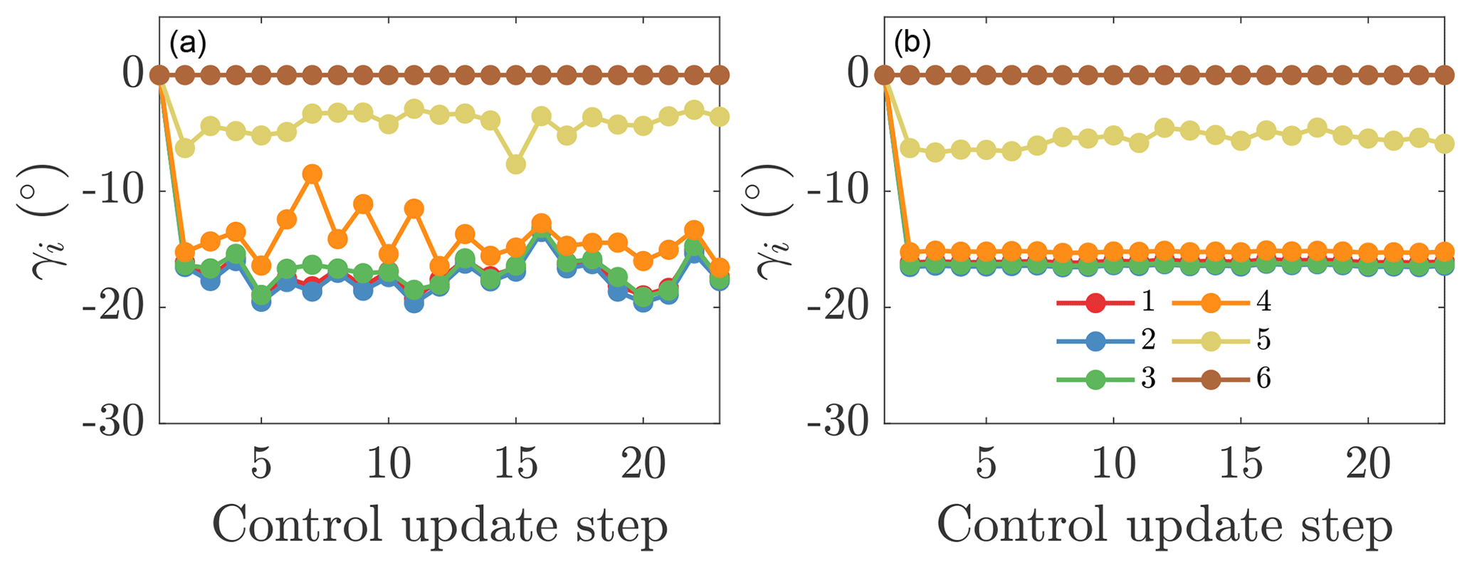
Figure E1 Yaw misalignment angles for each turbine in the wind farm for online control using (a) the initial parameters to initialize the next state (ND141) and (b) static state estimation parameters (ND142) for wind farm alignment at 14^∘.

Figure E2 Time-averaged wind farm power production as a function of the control update step for online control using (a) the initial parameters to initialize the next state (ND141) and (b) static state estimation parameters for wind farm alignment at 14^∘ (ND142). The wind farm power is normalized by the power production of the aligned wind farm case.