Change-point detection in wind turbine SCADA data for robust condition monitoring with normal behaviour models

Analysis of data from wind turbine supervisory control and data acquisition (SCADA) systems has attracted considerable research interest in recent years. Its predominant application is to monitor turbine condition without the need for additional sensing equipment. Most approaches apply semi-supervised anomaly detection methods, also called normal behaviour models, that require clean training data sets to establish healthy component baseline models. In practice, however, the presence of change points induced by malfunctions or maintenance actions poses a major challenge. Even though this problem is well described in literature, this contribution is the first to systematically evaluate and address the issue. A total of 600 signals from 33 turbines are analysed over an operational period of more than 2 years. During this time one-third of the signals were affected by change points, which highlights the necessity of an automated detection method. Kernel-based change-point detection methods have shown promising results in similar settings. We, therefore, introduce an appropriate SCADA data preprocessing procedure to ensure their feasibility and conduct comprehensive comparisons across several hyperparameter choices. The results show that the combination of Laplace kernels with a newly introduced bandwidth and regularisation-penalty selection heuristic robustly outperforms existing methods. More than 90 % of the signals were classified correctly regarding the presence or absence of change points, resulting in an F1 score of 0.86. For an automated change-point-free sequence selection, the most severe 60 % of all change points (CPs) could be automatically removed with a precision of more than 0.96 and therefore without any significant loss of training data. These results indicate that the algorithm can be a meaningful step towards automated SCADA data preprocessing, which is key for data-driven methods to reach their full potential. The algorithm is open source and its implementation in Python is publicly available.

1 Introduction

Wind energy plays a major role in the decarbonisation of energy systems around the world. It has developed into a mature technology over the past decades and its levelised cost of electricity (LCOE) has reached a competitive level (IRENA, 2019). At the same time costs for operation and maintenance (O&M), which account for approximately one-quarter of the LCOE, have seen only minor reductions (IRENA, 2019). An effective strategy to further reduce O&M costs is to switch from a scheduled maintenance scheme to condition-based maintenance. Under such a scheme maintenance decisions are based on information about the turbine's actual condition rather than on periodic inspections. The necessary information can be acquired through dedicated condition monitoring (CM) systems which can be for instance vibration-, oil-, or acoustic-emission-based (for a comprehensive review of state-of-the-art wind CM systems please refer to Coronado and Fischer, 2015). On the other hand, each wind turbine is equipped with a variety of sensors in its supervisory control and data acquisition (SCADA) system. Utilisation of operational SCADA data for CM has attracted considerable research interest since it provides insights with no need for additional equipment. A wide range of methods have proven to be able to detect developing malfunctions at an early stage, often months before they resulted in costly component failures (see e.g. Zaher et al., 2009; Schlechtingen and Santos, 2011; Bangalore et al., 2017; Bach-Andersen et al., 2017). For a comprehensive review refer to Tautz-Weinert and Watson (2016). SCADA data-based condition monitoring, therefore, represents a cost-efficient and effective complement to state-of-the-art CM-solutions.

Its primary task is to classify the state of a turbine or one of its components as either healthy or faulty. However, the available SCADA data represent predominantly healthy operation with no or only comparatively few instances of faulty condition. In such a setting semi-supervised anomaly detection, often called normal behaviour modelling, has proven to be useful (Chandola et al., 2009). Normal behaviour models (NBMs) are trained on healthy data to represent the class corresponding to the normal state. Subsequently, deviations between model output and the measured sensor values can be processed and evaluated to identify anomalies (compare Fig. 1). For wind turbines, performance and temperature monitoring can be distinguished. The former aims to detect abnormal deviations from the turbine's usual power output, whereas the latter aims to detect deviations from the healthy thermal equilibrium conditions. We will focus on temperature monitoring which is better suited for detecting malfunctions in the components along the drivetrain, which account for the majority of turbine downtime (compare Dao et al., 2019). Zaher et al. (2009) were among the first to apply the approach in the wind domain and prove its feasibility. Many publications with successful early detection of malfunctions followed (compare e.g. Butler et al., 2013; Kusiak and Verma, 2012; Sun et al., 2016; Bangalore et al., 2017; and Bach-Andersen et al., 2017.

Figure 1 Scheme of normal behaviour model-based anomaly detection with offline model preparation and online application.

Despite the promising NBM examples reported in literature, scaling the method to large fleets of wind turbines comes with practical challenges. Leahy et al. (2019) analysed 12 studies that apply the concept of NBM to wind turbine SCADA data and found that all but one reported significant manual efforts in data preprocessing due to data quality and data-access-related issues. That is why researchers have developed different filtering methods to ensure healthy training data without traces of malfunctions. They can be divided into domain-knowledge-based-, alarm-based-, work-order-based-, or statistical approaches (Leahy et al., 2019). Manual selection of representative operational patterns from the SCADA data sets would be an example of domain-knowledge-based filtering and can be found for instance in Zaher et al. (2009). Another common procedure is to filter NBM data against a certain threshold of active power production to exclude transitions between operational and non-operational states as well as corrupted sensor measurements during standstill (compare e.g. Sun et al., 2016; Bangalore et al., 2017; Tautz-Weinert, 2018). Schlechtingen and Santos (2011) were among the first to describe a more systematic semi-automated data preprocessing procedure. It consists of a domain-knowledge-based parameter range check, data scaling, handling of missing values, and lag removal. These measures have been extended by multivariate statistical filtering methods to automatically remove outliers (compare e.g. Bangalore et al., 2017).

However, a much more severe problem than missing, invalid, or poorly processed data is caused by structural changes in sensor measurements which have been reported in different publications (e.g. Schlechtingen and Santos, 2011 or Tautz-Weinert and Watson, 2017). They can be caused by sensor or component malfunctions as well as by maintenance actions. In an ideal setting, all potential causes would be quickly detected and corrected with the corresponding information being available to the respective data analyst. Unfortunately, this is rarely the case in practice (Tautz-Weinert and Watson, 2017, and Leahy et al., 2019), which has severe implications for NBMs. Trained on data containing abrupt changes in the underlying data-generating regime at a specific point in time (change point), NBMs are fit to multiple, potentially even faulty, states of operation, causing them to fail their intended task. Since change points (CPs) can make the NBM approach infeasible in practice, this has been identified as the most serious issue for their application (Tautz-Weinert and Watson, 2017).

Based on the findings described above this study aims to be the first to conduct a systematic analysis regarding the presence of CPs in SCADA signals. Moreover, an approach for robust detection of structural changes in SCADA measurements will be suggested. Non-parametric kernel-based change-point detection (CPD) methods will be adapted to the problem at hand. This includes recommendations for the choice of respective hyperparameters and useful signal preprocessing steps based on evaluation across a large range of SCADA signals from multiple wind farms. The result represents a step towards scalability of SCADA-based NBM, which is essential for the promising method to reach its full potential. The remainder of this paper is organised as follows: Sect. 2 presents the SCADA data used in this study and evaluates the presence and characteristics of CPs. Section 3 presents the method utilised in this study by formalising the CPD problem and introducing kernel-based CPD algorithms and their respective evaluation metrics. Section 4 specifies the CPD algorithm with its preprocessing steps and the selection of hyperparameters. Section 5 presents the performance over a range of hyperparameter configurations concerning different evaluation objectives followed by a discussion of results. Section 6 concludes with a summary and outlook.

2 Change points in wind turbine SCADA data

Wind turbine SCADA systems record measurements from sensors placed all over the turbine. Available signals usually include temperature measurements, electrical measures, pressure values, speed counters, timers, status parameters, and environmental conditions. Modern SCADA systems often record more than 100 different signals at sampling rates of 1 Hz. However, the typical temporal resolution available for analysis is 10 min average values due to data storage limitations and access restrictions. Change points in wind turbine SCADA signals can be induced by various causes. Generally, they can be sensor-, component-, or maintenance-related. Sensor-related structural breaks are often caused by sensor drifts, sensor failures, or malfunctions in the communication system. Component-related CPs can originate from changes in component physics or component failure. While sensor- and component-related CPs can be considered genuine faults, specific maintenance activities, such as changes in set points, are another common cause. The following sections first describe the SCADA data used in this study, the signal selection, and the CP annotation process. Subsequently, qualitative CP characteristics, their relation to potential causes, and their implications for detection are discussed. Finally, the presence of CPs in the data sets is evaluated quantitatively.

2.1 Data set and change-point annotation

For the current study SCADA data from 33 multi-megawatt turbines from different manufacturers were used. All turbines are equipped with gearboxes and double-fed induction generators and were commissioned later than 2013. They are located at three different sites of moderate complexity. For each turbine, SCADA data representing more than 2 full years of continuous operation within the first 5 years after commissioning were present. Each turbine's SCADA system records between 30 and 100 signals in the typical 10 min resolution. From the almost 2000 time series, 600 were selected for CPD based on the signal's potential for temperature monitoring using NBMs. Therefore, all power-train-related temperature and oil pressure values were selected. Additionally, temperatures from the pitch system, the electrical system, and ambient conditions were chosen. The pie chart on the left in Fig. 2 shows the allocation of the 600 analysed signals to the respective components. Generator and gearbox-related signals represent half of the overall selection. These components are also typically targeted by SCADA-based NBMs for temperature monitoring (compare Tautz-Weinert and Watson, 2016). The high number of pitch-related signals is due to the availability of multiple sensors in each blade's pitch system. A full list of the analysed signals and their mapping to the respective components can be found in Appendix B1. Next to the sensor time series, SCADA log files and information about major maintenance activities were present. They were combined with a visual inspection of all analysed signals to manually annotate CPs. The raw signals, their de-trended and normalised transformations (compare Sect. 4.1), and their summary statistics were compared using different temporal resolutions. The comparison of all signals related to the same component often led to coherent findings in the case of CP presence, which further increased confidence in the annotation. Moreover, signals were compared to their equivalent from at least five neighbouring turbines in the farm. This so-called trending approach is well known in SCADA analysis for monitoring wind turbines (compare Tautz-Weinert and Watson, 2016) and helped to highlight the difference between normal signal behaviour and abrupt changes. The results of this tedious task were reviewed by fellow researchers to secure the utmost objectivity and reduce the number of false annotations to a minimum.

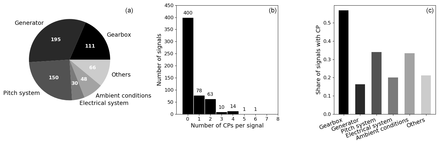
Figure 2 Number of signals per component (a), number of CPs per signal (b), and share of signals with CPs per component (c) for the full 2-year time horizon.

2.2 Qualitative change-point evaluation

Structural changes in SCADA signals manifest themselves in a wide range of different signal behaviours. This is due to the multitude of potential causes in combination with the unique statistical nature of each signal. Often the cause of a change point is closely related to how it manifests itself in the signal. Changes in signal behaviour can, for instance, be classified as permanent or temporary. Temporary changes consist of two CPs, where signal behaviour returns to its original pattern after a limited period (usually not longer than an interval of periodic inspections). For such changes, it is very common that the first CP was caused by a malfunction or fault which was consecutively fixed by a corrective maintenance action. A permanent change in signal behaviour, on the other hand, is not reverted and more likely to be attributed to a preventive maintenance action or control changes. However, there still is the possibility of a permanent change being induced by a fault which has either not been discovered or has not been considered to be severe enough to fix. Another distinction can be made between gradual and abrupt changes. Gradual changes can almost exclusively be attributed to be fault-related whereas abrupt changes could be either. Furthermore, some physics of failure considerations might explain the nature of an observed change. For temperature measurements, for instance, it is rather unlikely that a component failure manifests itself in overall lower temperatures. For sensors like oil pressure measurements, the exact opposite would be the case. Figure 3 shows three exemplary types of structural changes in different SCADA signals. To highlight the changes, non-operational data were excluded, and the signals were normalised with their respective median to facilitate a comparison. Figure 3a shows a gearbox bearing temperature. The CP in February of the depicted year is easy to recognise. It occurred after a scheduled maintenance during which a cooling fluid was exchanged, and the bearing consequently operates at clearly elevated temperatures. Figure 3b displays a turbine's hydraulic oil temperature for 2 years. A hydraulic fault in October of the second depicted year of operation causes the temperature to steadily rise compared to pre-CP conditions. Lastly, Fig. 3c shows a gear oil pressure signal over 1 year. The signal shows a temporary decline of a turbine's gear oil inlet pressure and its return to the initial level. This was caused by an issue with the lubrication oil filter which was fixed during a scheduled maintenance activity. A unifying framework to detect changes in SCADA measurements has to account for this diversity of signals and changes.

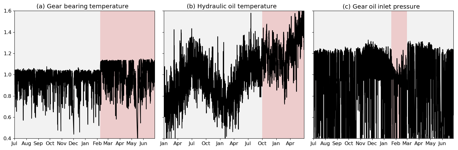
Figure 3 Exemplary SCADA signals exposing different structural changes. Each change in background colour indicates a CP.

When formalising the CP detection problem in the next chapter it will become clear that the individual CP characteristics translate into how statistically distinct and therefore how easy to detect a CP is. Next to the decisive ratio between the magnitude of change and the individual signal variance or noise level (Garreau, 2017), qualitative characteristics play a major role too. Permanent changes are for example easier to detect than short temporary ones. Also, abrupt changes are generally easier to detect than slowly developing gradual changes, especially when it comes to exact temporal localisation.

2.3 Quantitative CP evaluation

Figure 2 shows the results of the quantitative CP evaluation. The central chart represents a histogram over the number of CPs per signal. Exactly one-third of the analysed signals were affected by changes over the approximately 2.5-year period. Generally, only a few CPs were found per signal. Less than 5 % of the affected signals exhibit three or more CPs. Figure 2c compares the share of signals corrupted by changes for each component category. Gearbox-related signals are most affected, with more than half the signals containing CPs. For pitch-related and ambient condition signals around 30 % of the time series were found to be affected. The high number of pitch-related CPs were caused by systematic disturbances in the pitch motor temperature sensors in one of the wind farms. In the case of ambient conditions, a range of temperature sensors was found to be affected by severe drifts. Even though these findings might vary across different turbine types, ages, and site conditions, the order of magnitude of CP presence found in this study highlights the necessity of a robust CPD methodology. The presented figures reflect the CP summary statistics across the selected signals for the full period where data were available. Additionally, each of the 600 signals was divided exactly in the middle, resulting in 1200 sub-signals each covering approximately 1 year of operation. A 2-year signal that contains only one CP, therefore, results in one signal with and one signal without a CP. The respective summary statistics of the 1-year signals can be found in Appendix A1. The algorithm will be evaluated on both the 2-year and the 1-year signals to ensure its generalisation abilities over different signal lengths. Moreover, a period of 1 year seems to be closer to the current practice of NBM training data selection which represents the algorithm's target application (compare Letzgus, 2019).

3 Method for change-point detection

The detection of CPs in time series is a well-studied problem in statistics, signal processing, and machine learning (ML). The goal is to detect time instants at which the underlying data generation process and therefore the marginal distribution of the observations change abruptly. In other words, the time series is to be split into statistically homogeneous segments (Brodsky and Darkhovsky, 1993). First works date back to the 1950s (e.g. Page, 1955), but the topic has stayed the subject of active research until today, with methods being further refined and applied to many different domains, such as remote sensing (Touati et al., 2019), audio signal processing (Rybach et al., 2009), or medical condition monitoring (Malladi et al., 2013). Refer to Aminikhanghahi and Cook (2017) for an overview of time series CPD methods. The following section will describe, classify, and formalise the CP problem at hand based on Brodsky and Darkhovsky (1993).

3.1 Problem formulation

Conceptually, the CPD problem can be divided into online and offline detection. The former, sometimes also referred to as sequential CP detection, aims to identify changes in real-time settings as early and confidently as possible. In contrast, the latter, also known as signal segmentation, aims to determine the CP a posteriori with the data acquisition process being completed at the time that the homogeneity hypothesis is checked. Offline CP problems can be further classified with respect to the a priori knowledge of the respective task. Complexity is significantly lower if the number of true CPs is known, which reduces the task to the precise estimation of their location. In most real-world applications, however, the number of CPs itself has to be estimated. The same applies for a priori information about the statistical characteristics of the respective signals. Prior knowledge allows for assumptions regarding the family of underlying distributions. Therefore, CPs can be detected by identifying a change in the parameters describing the distribution. Non-parametric methods, on the other hand, require no such prior information, which makes them more flexible and therefore often better suited for real-world problems. The present task of ensuring CP-free training data sets represents an offline CPD problem, where the number of true CPs is unknown. Even though it is expected that many SCADA signals are not affected by structural changes, more than one statistically homogeneous segment per signal may exist (compare Fig. 2b). Lastly, the SCADA data set consists of various statistically different signals which do not allow for unifying assumptions regarding their family of distributions. Therefore, non-parametric methods will be applied.

Let us formalise the given problem under the prevailing conditions. We assume $X=\mathit{\{}{X}_{\mathrm{1}},X_{\mathrm{2}},\mathrm{\dots },X_T\mathit{\}}$ to be a piece-wise stationary time series signal in ℝ^d consisting of T observations. Piece-wise stationarity implies that X can be divided into N (N≥1) segments where each segment is well described by some distribution which might differ for consecutive segments. The segments therefore represent homogeneous sets s which are characterised by N−1 CPs at some unknown instants in time ${\mathit{\tau }}_{\mathrm{1}}^{*}<{\mathit{\tau }}_{\mathrm{2}}^{*}<\mathrm{\dots }<{\mathit{\tau }}_{N-\mathrm{1}}^{*}$ (compare Eq. 1). Now, CP detection can be formulated as a model selection problem where the CPs τ are the model parameters to be estimated. This can be achieved by defining a cost function C(τ) that quantifies intra-segment dissimilarity with respect to the chosen CPs τ (compare Eq. 2). A naive minimisation of this cost function would result in a segmentation into N segments of unit size. Therefore, a regularisation term (𝒫(τ)) was proposed for example by Lavielle (2005) which penalises for every additional CP and therefore reduces complexity of the segmentation (compare Eq. 2).

$$\begin{array}{}\text{(1)}& {\displaystyle }\begin{array}{rl}s& =\mathit{\{}{s}_{\mathrm{1}},s_{\mathrm{2}},\mathrm{\dots },s_N\mathit{\}}=\mathit{\left\{}\mathit{\right\{}{X}_{\mathrm{0}},\mathrm{\dots },X_{{\mathit{\tau }}_{\mathrm{1}}}\mathit{\}},\\ & \mathit{\{}{X}_{{\mathit{\tau }}_{\mathrm{1}}+\mathrm{1}},\mathrm{\dots },X_{{\mathit{\tau }}_{\mathrm{2}}}\mathit{\}},\mathrm{\dots },\mathit{\{}{X}_{{\mathit{\tau }}_{N-\mathrm{1}}},\mathrm{\dots },X_T\mathit{\}}\mathit{\}}\end{array}\text{(2)}& {\displaystyle }\widehat{\mathit{\tau }}\mathit{ϵ}\underset{\mathit{\tau }}{\mathrm{argmin}}C\left(\mathit{\tau }\right)+\mathcal{P}\left(\mathit{\tau }\right)\text{where}C\left(\mathit{\tau }\right)=\sum _{n=\mathrm{1}}^{N}C\left(s_n\right)\end{array}$$

Since the complexity of the optimisation problem grows quadratically with the number of data points, a naive approach for minimising the cost function C(τ) can be computationally expensive. Several approximate search methods like a sliding window or binary segmentation were developed (compare Truong et al., 2020). They come with benefits regarding computing time but naturally compromise on precision. The optimal solution can still be obtained efficiently by applying an algorithm based on dynamic programming. It was originally introduced in 1958 (Bellman, 1958) for solving a shortest-path problem for traffic networks. Since then the algorithm has been developed further (see e.g. Guédon, 2013) and was successfully applied in the context of CPD. The method utilises the additive structure of the cost objective to recursively compute optimal CPs for multiple sub-signals among which the global minimum is then selected. An implementation of the algorithm is publicly available as part of the CP detection library ruptures in Python (Truong et al., 2020) and was utilised within this study.

3.2 Kernel-based change-point detection

Equation (2) represents a general cost function for solving the signal segmentation task at hand but the result heavily depends on an appropriate measure for the intra-segment similarity. Harchaoui and Cappé (2007) proposed a kernel-based approach which does not rely on parametric assumptions but can detect changes in the high-order moments of the signal distribution. Kernel methods use mapping functions $\mathrm{\Phi }:{\mathbb{R}}^d\to \mathcal{H}$ to implicitly project a signal into a potentially much higher-dimensional reproducing kernel Hilbert space (Schölkopf and Smola, 2002). With the well-known kernel trick, the distance or similarity of two data points in the high-dimensional feature space can be calculated by directly applying the kernel function (compare Eq. 3). Harchaoui and Cappé (2007) used this property to evaluate the adequacy of τ. They define a kernel least-squares criterion that measures the intra-segment scatter (see Eq. 4). Intuitively, the second term of Eq. (4) increases if the chosen segments are more similar to each other and in return maximises dissimilarity between segments due to the negative sign. Note that the intra-segment scatter requires the calculation of the kernel-gram matrix $G_{i,j}=K(X_i,X_j)$, which implies a quadratic computational complexity and therefore restricts the method regarding the size of the data sets. By minimising the criterion the best segmentation for a known number of CPs can be obtained. Conceptually, any positive semi-definite kernel can be applied in this framework. Popular candidates are the linear (i), Laplacian (ii), or Gaussian (iii) kernel (compare Eq. 5). Note that Laplacian and Gaussian kernels need the selection of an appropriate bandwidth parameter h. Arlot et al. (2019) expanded the method to an unknown number of CPs by applying the concept of penalising for additional CPs (compare Eq. 2). Since then the kernel-based algorithm has been successfully applied to multiple real-world time series CPD problems (compare with Arlot et al., 2019).

$$\begin{array}{}\text{(3)}& {\displaystyle }k(x,x^{\prime })=\langle \mathrm{\Phi }\left(x\right),\mathrm{\Phi }(x^{\prime }{)}_{\mathcal{H}}\rangle \text{and}k(x,x)={∥\mathrm{\Phi }\left(x\right)∥}_{\mathcal{H}}^{\mathrm{2}}\text{(4)}& {\displaystyle }\begin{array}{rl}& C\left(\mathit{\tau }\right)={\displaystyle \frac{\mathrm{1}}{T}}\sum _{t=\mathrm{1}}^{T}k(X_t,X_t)\\ & -{\displaystyle \frac{\mathrm{1}}{T}}\sum _{n=\mathrm{1}}^N\left[{\displaystyle \frac{\mathrm{1}}{{\mathit{\tau }}_n-{\mathit{\tau }}_{n-\mathrm{1}}}}\sum _{i={\mathit{\tau }}_{n-\mathrm{1}}+\mathrm{1}}^{{\mathit{\tau }}_n}\sum _{j={\mathit{\tau }}_{n-\mathrm{1}}+\mathrm{1}}^{{\mathit{\tau }}_n}k(X_i,X_j)\right]\\ & {\mathit{\tau }}_{\mathrm{0}}=\mathrm{0}\end{array}\text{(5)}& {\displaystyle }\begin{array}{rl}& \left(\mathrm{i}\right)k_{\mathrm{lin}}(x,y)=\langle x,y\rangle \left(\mathrm{ii}\right)k_{\mathrm{lp}}(x,y)=\exp \left({\displaystyle \frac{-\Vert x-y\Vert }{h}}\right)\\ & \left(\mathrm{iii}\right)k_{\mathrm{rbf}}(x,y)=\exp \left({\displaystyle \frac{-\Vert x-y{\Vert }^{\mathrm{2}}}{h}}\right)\end{array}\end{array}$$

3.3 Performance evaluation

The performance of CPD algorithms can be evaluated using the classic notation of true positives (TPs), false positives (FPs), true negatives (TNs), and false negatives (FNs). To appropriately interpret the evaluation results, the implications of false classifications have to be considered. In the case of NBMs, a FN translates into a risk for model quality and a FP into loss of potentially valuable training data. However, the individual impact depends on the severity of the change, meaning the degree of distinction from normal signal behaviour as well as the duration of its presence. This goes well with the concept of the presented CPD algorithm since the notion of severity directly translates into a cost reduction by segmentation. For the concrete evaluation of CPD results two different evaluation objectives are distinguished:

1. automatic training data validation (detect the presence of CP in a given processed signal) and

2. automatic training sequence selection (detect the number and exact location of CPs in the processed signal).

Automatic training data validation answers whether a CP is present in a given SCADA signal or not. Therefore, the CP detection result is evaluated once for each signal. If the algorithm indicates one or more CPs for a signal containing at least one CP, the result is evaluated as a true positive. No CP detection in a CP-free signal represents a true negative. In practice, this means that a CP detection result is evaluated as a true positive, even if the number and location of indicated CPs do not necessarily represent the ground truth. Nevertheless, this can be useful information for validating signals against the presence of CPs. In particular, since the alternative is a full manual inspection of all signals. Automatic training data validation, therefore, preselects the signals for visual inspection in which the actual locations of the CPs are subsequently determined. The next step towards a fully automated NBM approach is automated training sequence selection. This requires a more precise evaluation for each CP and each CP indication individually. Therefore, an acceptable margin is selected around each true CP in which a detection is evaluated as a TP. While for automatic training data validation this margin was practically set to infinity, a fixed number of days has to be chosen for automatic training sequence selection. A CP which is present in the signal but not indicated by the algorithm is evaluated as a FN. Detection outside the margin boundaries represents a FP. A TN represents a CP-free signal with no detection. The concept is visualised in Fig. 4 where a TP, FP, and FN are depicted. Note that a CP indicated just outside the margin already leads to a “double” punishment by evaluating the indication as a FP and the true CP as not detected (FN). Intuitively, the overall detection result depends on the selected acceptable margin. Moreover, the margin corresponds to the amount of data around the detected CP to be automatically cut off in automated training data selection and therefore to a trade-off between data loss and accuracy. In this paper, the acceptable margin was selected to be ±60 d around the true CP. The choice is motivated by the fact that missing a dominant true CP can be more critical for many applications, such as NBM for example, than a reduction of training data by the given period. Moreover, this is attributed to potential inaccuracy during the manual annotation process in the case of uncertainty about the exact temporal localisation of the change (compare Sect. 2.1). With the classification of each detected CP into true or false positive or negative, the well-known evaluation metrics accuracy, precision, recall, and F1 score can be calculated (compare Eqs. 6–7).

$$\begin{array}{}\text{(6)}& {\displaystyle }\begin{array}{rl}& \text{Accuracy}={\displaystyle \frac{\mathit{\#}\mathrm{TP}+\mathit{\#}\mathrm{TN}}{\mathit{\#}\mathrm{TP}+\mathit{\#}\mathrm{TN}+\mathit{\#}\mathrm{FP}+\mathit{\#}\mathrm{FN}}}\\ & \text{Precision}={\displaystyle \frac{\mathit{\#}\mathrm{TP}}{\mathit{\#}\mathrm{TP}+\mathit{\#}\mathrm{FP}}}\\ & \text{Recall}={\displaystyle \frac{\mathit{\#}\mathrm{TP}}{\mathit{\#}\mathrm{TP}+\mathit{\#}\mathrm{FN}}}\end{array}\text{(7)}& {\displaystyle }\text{F1 score}=\mathrm{2}\cdot {\displaystyle \frac{\text{precision}\cdot \text{recall}}{\text{precision}+\text{recall}}}\end{array}$$

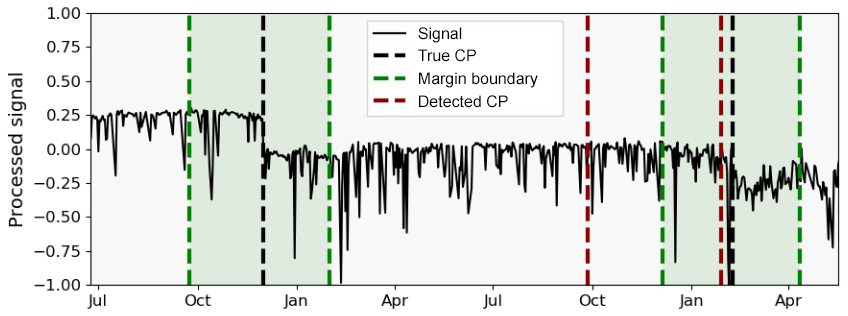
Figure 4 Exemplary evaluation of a CP detection result with one FN (December, first year), FP (September, second year), and TP (February, second year).

4 Algorithm for change-point detection

This section describes the detailed steps of signal processing applied to detect the CPs in this study. Signal preprocessing, as well as the choice of hyperparameters, is discussed.

4.1 Data preprocessing

Wind turbine operation is highly volatile due to intermittent ambient conditions. This is reflected in the high variance of raw SCADA measurements and complicates CP detection because the change in signal behaviour might be small in relation to regular signal behaviour. Signal preprocessing methods can help to reduce the signal to its most valuable components for CP detection and therefore facilitate the process. Tautz-Weinert and Watson (2017) suggest comparing monthly maximums and percentiles to detect structural changes. This was found to be too granular to attribute for temporary changes of less than 1 month. Additionally, such an approach does not reduce seasonality, which was found to be an important factor for successful kernel CPD. Instead, the following preprocessing steps were taken in this study:

• removal of non-operational periods,

• normalisation with operational state and ambient conditions,

• resampling with reduced temporal resolution.

The removal of non-operational periods is a routine preprocessing step in SCADA data analysis (compare e.g. Sun et al., 2016; Bangalore et al., 2017; Tautz-Weinert, 2018) and was motivated by the reasoning that changes in operational conditions will become most apparent when the turbine is in operation. Also, it was observed that sensor values during non-operational periods, e.g. during maintenance, sometimes take predefined standard values. To exclude such distorting effects, all data points where the turbine is operating on less than 10 % of its rated power were excluded. Furthermore, the signal measurements were normalised based on the prevailing operating conditions. Active power production and rotor rotational speed were found to be the most dominant to characterise the turbine's operational state. Ambient temperature was identified to be a good regressor to exclude seasonality from the sensor measurements. Therefore, each signal was normalised using these three input variables in a linear regression (compare Eq. 8). The model was found to adequately subtract the influences of external conditions, is computationally cheap, and due to its simplicity does not allow overfitting of the sensor signals. In a last step, the normalised signal was averaged over each day, if at least 3 h of operational data were available. This allows the extraction of the normalised signal characteristics and additionally reduces the number of data points, which facilitates the computation of the kernel gram matrix. An exemplary result of the preprocessing procedure is shown in Fig. 5. It displays the three signals shown earlier (compare Fig. 3), after preprocessing. Note in particular how the method facilitates a clear identification of the CP in the hydraulic oil temperature compared to the raw signal.

$$\begin{array}{}\text{(8)}& \begin{array}{rl}{\text{signal}}^{*}& =f(X_P,X_{\mathrm{rpm}},X_{T_{\mathrm{amb}}})\\ & =w_{\mathrm{1}}\cdot X_P+w_{\mathrm{2}}\cdot X_{\mathrm{rpm}}+w_{\mathrm{3}}\cdot X_{T_{\mathrm{amb}}}+c\end{array}\end{array}$$

Figure 5 Exemplary SCADA signals after preprocessing (compare Fig. 3). Each change in background colour indicates a CP.

A minor disadvantage of this approach is that the regressing signals, meaning active power, rotor speed, and ambient temperature, cannot be preprocessed the same way. In fact, abrupt change in one of the regressors can induce a CP in highly correlated signals. In this study, such a case occurred a few times when the ambient temperature sensor of a turbine was corrupted. However, regressing the inputs themselves with signals from neighbouring turbines first and then running the algorithm on them to check for CPs can exclude those cases. Alternatively, a simple rule checking for simultaneous CP detections in all signals particularly correlated to the same regressor can do the trick as well.

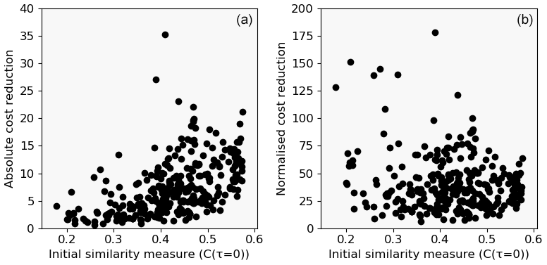
Figure 6 Absolute (a) and normalised (b) cost reduction of healthy signals by imposing one CP versus average cost.

4.2 Choice of hyperparameters

The CPD method described in Sect. 3 requires adequate selection of several hyperparameters, namely the type of kernel, its respective bandwidth, and the penalty term for additional CPs. All three were found to have a profound impact on the CPD performance. Choosing an appropriate kernel is a well-studied problem by itself in many applications. In the context of CPD the widely used linear, Gaussian, and Laplacian kernels have been used (Garreau, 2017). Therefore, all three will be compared within this study. The choice of an adequate bandwidth h is another problem often encountered when working with kernel methods. Looking at the definition of the Gaussian and the Laplacian kernels (see Eq. 5), it becomes clear that a bandwidth chosen too large or too small will make the entries of the gram matrix go towards zero or 1 respectively, and therefore valuable information will be lost. A common approach is therefore to choose the bandwidth in the range of the calculated distances. Gretton et al. (2012) for example suggest a median heuristic in the context of a kernel two-sample test (compare Eq. 9). This heuristic is heavily used in ML literature (Garreau, 2017) and is also applied in the CPD settings (Truong et al., 2020). Arlot et al. (2019) on the other hand suggest using the empirical standard deviation of the signal itself as the bandwidth. Both choices of bandwidths, h_median and h_SD, are tested and compared in this paper (compare Eq. 9). Furthermore, it is argued here that estimation of an appropriate bandwidth based on a signal with abruptly changing properties might lead to a non-optimal choice. Therefore, a third approach is being introduced and tested where the signal is divided into k different segments $S_{\mathrm{bw}}=\mathit{\left\{}\mathit{\right\{}{X}_{\mathrm{0}}\mathrm{\dots }{X}_t\mathit{\}},\mathrm{\dots },\mathit{\{}{X}_{(k-\mathrm{1})\cdot t+\mathrm{1}}\mathrm{\dots }{X}_{k\cdot t}\mathit{\left\}}\mathit{\right\}}$ of equal length t, and the empirical standard deviation is calculated for each segment. The bandwidth is consequently chosen as the maximum of the k standard deviations. In this study, k is selected to be 20. Consequently, each segment consists of roughly 3 to 5 weeks of operational data. For the remainder of the paper, approach (c) is referred to as batch-SD bandwidth.

$$\begin{array}{}\text{(9a)}& {\displaystyle }h=\text{median}(\Vert X_i-X_j{\Vert }^n)\text{(9b)}& {\displaystyle }h=\mathrm{SD}\left(X\right)\text{(9c)}& {\displaystyle }h=\text{max}\left(\mathrm{SD}\right(S_{\mathrm{bw}}\left)\right)\end{array}$$

Another crucial hyperparameter choice is the selection of an appropriate penalty term (compare Eq. 2) which controls the number of CPs to be detected by the algorithm. If the penalty is selected too low, too many CPs will be detected and vice versa. A data-driven approach for choosing the penalty in the context of minimisation of a penalised criterion is the so-called slope heuristic (Birgé and Massart, 2007). It was shown that the optimal penalty to avoid overfitting is approximately proportional to a minimal penalty which can be obtained based on a regression between the penalised quantity and the associated cost function without penalisation. In the context of CP detection this was firstly described by Lebarbier (2002), further refined by Baudry et al. (2012) and applied by Arlot et al. (2019). They suggest a minimal penalty based on two constants s₁ and s₂ which are obtained by regressing the cost function C(τ_n) against $\log \left(\genfrac{}{}{0ex}{}{T-\mathrm{1}}{n-\mathrm{1}}\right))$ as well as $\frac{n}{T}$. T corresponds to the total number of data points and $n\in [\mathrm{0.6}\cdot N_{\max },N_{\max }]$, where N_max is an estimation of the maximal number of segments N (compare Eq. 1). Based on our findings from Fig. 2, we chose N_max=6. Finally, the minimum penalty is multiplied with the factor α to obtain the final optimal penalty (compare Eq. 10). Even though the optimal choice of α is problem specific, α=2 was reported as a suitable choice by Arlot et al. (2019).

$$\begin{array}{}\text{(10)}& {\mathrm{pen}}_{\mathrm{opt}-\mathrm{slope}}\left({\mathit{\tau }}_n\right)={\mathit{\alpha }}_{\mathrm{slope}}\cdot {\displaystyle \frac{\mathrm{1}}{T}}\cdot (-s_{\mathrm{1}}\cdot \log \left(\genfrac{}{}{0ex}{}{T-\mathrm{1}}{n-\mathrm{1}}\right)-s_{\mathrm{2}}n)\end{array}$$

In this study, the slope heuristic is compared to a simpler approach chosen based on the following consideration: signals which are inherently similar to themselves are by default characterised by a relatively low initial cost value and vice versa. This means that each CP by default leads to a larger cost reduction for more dissimilar signals. Therefore, the penalty term is chosen based on the sum of costs without any CP (compare Eq. 11). Figure 6 supports this reasoning. Here, a CP was enforced on all signals without changes. The resulting reduction in the cost function is shown over the initial average cost (panel a). An approximately quadratic relation between cost reduction and initial average cost can be observed. Figure 6b shows the relative reduction normalised with C(τ=0)². Consequently, the normalised cost reductions are distributed much more uniformly and facilitate the selection of a single penalty value over all signals. Moreover, the penalty term can now be easily calculated from the signal characteristic itself. This is considered an advantage over the more complex methods found in literature. The findings indicate that a reasonable choice of the penalty factor α_cost would be in the range between 75 and 150 for a Laplace kernel with a bandwidth selected according to the batch-SD heuristic. A penalty factor larger than 200 can be considered a conservative choice with only a few false positives. Conversely, the reduction of the cost function induced by a CP can be interpreted as a confidence measure. Note that these values depend on the kernel configuration.

$$\begin{array}{}\text{(11)}& {\mathrm{pen}}_{\mathrm{opt}-\mathrm{cost}}\left(\mathit{\tau }\right)={\mathit{\alpha }}_{\mathrm{cost}}\cdot C(\mathit{\tau }=\mathrm{0}{)}^{\mathrm{2}}\end{array}$$

5 Results for change-point detection

The result section presents the algorithm's performance on automatic training data validation and selection. For both evaluation objectives, different hyperparameter configurations in terms of kernel-, bandwidth-, and penalty selection are compared. Additionally, the effect of signal length is investigated to ensure the algorithm's generalisation abilities. Results are analysed on a cumulative as well as on a component level. Finally, the results are discussed and implications for the algorithm's practical application derived.

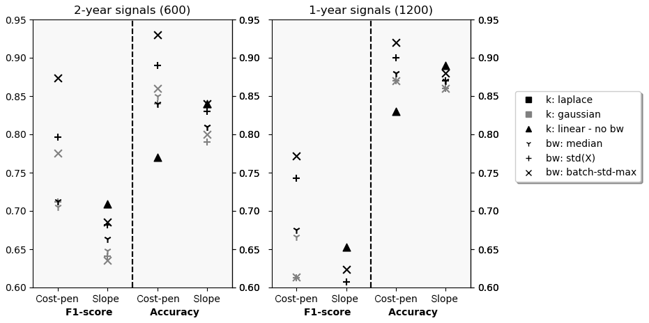
Figure 7 Validation F1 score and accuracy for different hyperparameter configurations on 2-year and 1-year signals.

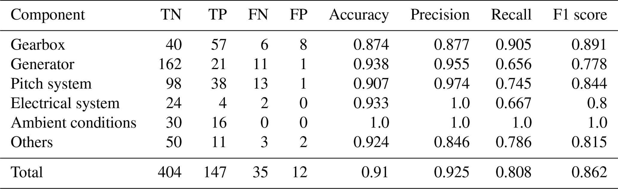
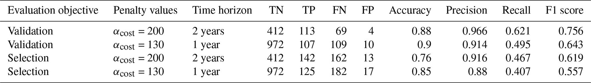
Table 1 Automated training data validation results per component for best configuration (Laplace/batch-SD/ α_cost=145) on 2-year signals.

5.1 Evaluation of automated training data validation

In this section, the algorithm's ability to distinguish between signals with and without CPs is evaluated. Figure 7 shows the results achieved by different configurations on the full 2-year signal length (left) and the 1-year signal length (right). Both F1 and accuracy scores are compared for different kernels, bandwidth choices, and penalty selection schemes. A clear ranking can be identified when comparing kernels. For configurations with cost-based penalties, Laplacian kernels perform best followed by Gaussian kernels. Linear kernels perform much worse. For penalties chosen according to the slope heuristic, the contrary is the case. Linear kernels perform best, closely followed by Laplace and Gaussian configurations. In terms of bandwidth selection, the intra-kernel ranking differs, but the leading Laplacian configurations use the batch-SD heuristic, which outperforms established standard deviation or median heuristics. When comparing penalty selection schemes, the cost-based penalty estimation suggested in this paper performs better than the slope heuristic. All discussed qualitative observations hold for both time horizons. However, a clear performance loss in terms of F1 score for the shorter signals can be observed. This is attributed to the design of the evaluation scheme. Firstly, there is a shift in the distribution between affected and not affected signals (compare Figs. 2 and Appendix A). Secondly, when the 2-year signal contains multiple CPs, detection of only the most significant one is enough for the signal to be evaluated as correctly classified (TP). When splitting this 2-year signal into two 1-year signals to analyse and evaluate them separately, detection of a less severe change in one of the signals might be required for both signals to be evaluated as correctly classified (both TP).

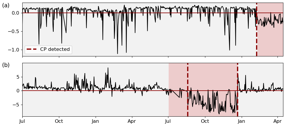
Figure 8 Examples of successful CP detection in gear oil pressure (a) and nacelle temperature (b). Each change in background colour indicates a true CP; each dashed line indicates a detected CP.

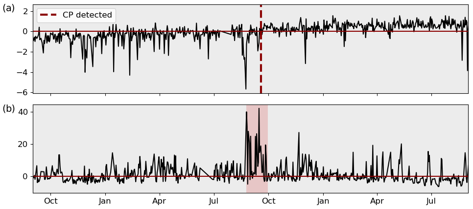
Figure 9 Examples of misclassification in gearbox (a) and generator (b) bearing temperature. Each change in background colour indicates a true CP; each dashed line indicates a detected CP.

In absolute terms, the overall best-performing configurations can classify more than 90 % of the signals correctly regarding the presence or absence of CPs. The wrongly classified signals are approximately one-quarter false positives and three-quarters false negatives. This translates into F1 scores of 0.87 and 0.76 for the different signal lengths. This performance is reached for a penalty factor of ${\mathit{\alpha }}_{{\mathrm{cost}}_{\mathrm{2}}}=\mathrm{145}$ and ${\mathit{\alpha }}_{{\mathrm{cost}}_{\mathrm{1}}}=\mathrm{80}$ respectively. The best results for both time horizons using the slope heuristic for penalty selection was achieved for penalty factors of α_slope=12.5, which is much higher than the α_slope=2 suggested in literature. At the same time, F1 scores range around 20 % behind the leading cost-penalty-based configuration. Table 1 displays the overall results as well as the results per component for the best-performing CPD configuration on the 2-year signals in detail. The algorithm reaches high performance across components. Ambient condition signals, as well as gearbox- and pitch-related signals, were classified with particularly high accuracy. Correctly classified CPs are often characterised by sharp transitions between the states and a significant difference in relation to the regular signal noise. Examples of successful detections can be found in Fig. 8. The top chart shows the correctly classified change in gear oil pressure after maintenance. The second chart shows the correctly identified shift and its return to normal behaviour in a nacelle temperature signal which was induced by problems in the generator cooling system and its consecutive fix. At the same time, there is a relatively high number of false positives for gearbox-related signals. This is mostly caused by bearing temperatures that are gradually rising due to normal wear (compare Fig. 9a). The algorithm detects the drift in the signal's distribution which, under the given evaluation framework, represents a false positive. In the broader context of NBM, this information is still valuable since it highlights the need for periodical model retraining. False negatives were mostly caused by short temporary changes which were not pronounced enough to compensate for the penalty of two CPs, which would be required to flag them correctly. An example is shown in Fig. 9b which depicts a generator bearing with temporary high temperatures. The detailed results for all configurations by penalty and time horizon can be found in Appendix C.

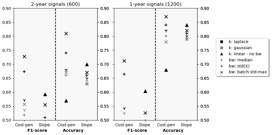
Figure 10 Selection F1 score and accuracy for different hyperparameter configurations on 2-year and 1-year signals.

Table 2 Automated training data selection results per component for best configuration (Laplace/SD-max/α_cost=150) on 2-year signals.

5.2 Evaluation of automated training sequence selection

In this section, the algorithm's ability to automatically select periods without CPs for each signal is analysed. Therefore, performance is evaluated for each CP individually rather than for each signal (compare Sect. 3.3). Figure 10 shows the CPD results analogously to the results for automated training validation in the previous section. Qualitatively, the findings concerning kernel selection and configuration are equivalent. Laplace kernels with batch-SD bandwidths perform best. In comparison with the results from the previous section, the more difficult evaluation objective manifests itself in overall lower performance scores. Even though accuracies reach well above 80 %, F1 scores drop to 0.73 and 0.71 for the two time horizons. However, the performance between the two analysed time horizons is very similar, which attributes for the algorithm’s ability to generalise across different signal lengths. The optimal penalty factors remain time horizon specific but stable across evaluation metric with ${\mathit{\alpha }}_{{\mathrm{cost}}_{\mathrm{2}}}=\mathrm{150}$ and ${\mathit{\alpha }}_{{\mathrm{cost}}_{\mathrm{1}}}=\mathrm{80}$. The general advantage of cost-based penalties is preserved with F1 scores approximately 15 % above the best slope-heuristic results which are achieved at ${\mathit{\alpha }}_{{\mathrm{slope}}_{\mathrm{2}}}=\mathrm{11.5}$ and ${\mathit{\alpha }}_{{\mathrm{slope}}_{\mathrm{1}}}=\mathrm{4}$.

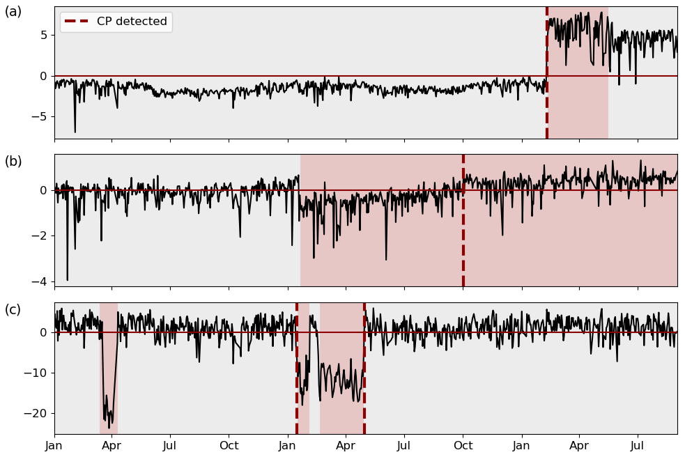
Figure 11 Examples of partially correct classified oil temperature (a), gearbox bearing temperature (b), and pitch motor winding temperature (c). Each change in background colour indicates a true CP; each dashed line indicates a detected CP.

Table 2 displays the overall results as well as the results per component for the best-performing CPD configuration on the 2-year signals in detail. To explain the drop in F1 score, the different false classifications of each component were analysed. Gearboxes show a relatively high number of both FNs and FPs. Approximately 50 % of the FNs can be attributed to the coexistence of large and comparatively small changes in the same signal. An example is shown in Fig. 11a where an oil temperature signal undergoes two significant changes with the second one not being detected. The initial dissimilarity, based on which the penalty is calculated, is dominated by the first change, and therefore detection of the second change cannot compensate for the high penalty value. Another 20 % of the gearbox-related FNs are caused by short temporary changes and a further 20 % by detections outside the 60 d margin (compare e.g. the gearbox bearing temperature in Fig. 11b). These represent at the same time approximately 25 % of the FPs. However, the majority of gearbox-related FPs are caused by the described signal drifts due to normal wear in gearbox bearings (compare Fig. 9a). At the same time around two-thirds of CPs are correctly detected in gearbox-related signals, often representing major changes such as a drop in gear oil pressure after maintenance (compare Fig. 8a). For the generator-related signals the main cause of FNs are relatively short temporary changes, such as the temporary high temperatures in a generator bearing displayed in Fig. 9b. The same reason causes the majority of FNs in pitch-related signals (35 out of the 40 false negatives were of the kind shown in Fig. 11c). These shifts in pitch motor winding temperature signals were caused by systematic communication problems. At the same time, many shifts were distinct enough to be detected, which explains the high number of TPs in pitch-related signals. It can be summarised that signal changes due to normal wear, temporary changes, and the coexistence of CPs with different significance levels represent challenges which have to be addressed in the future. Nevertheless, the algorithm gives reasonable results and was able to identify the majority of CPs present in the signals. The detailed results per component of all configurations by penalty and time horizon can be found in Appendix C.

5.3 Discussion of preprocessing, results, and application

From the presented results it can be concluded that Laplacian kernels in combination with bandwidths chosen based on the batch-SD heuristic are best suited for the problem at hand. This configuration in combination with cost-based penalties clearly outperformed all other configurations. Analysis showed that correctly classified CPs are often characterised by a permanent nature, sharp transitions between states, and a significant difference in relation to the regular signal noise. The latter two qualities are particularly amplified by the preprocessing procedure (compare Sect. 4.1). To demonstrate its importance, the algorithm was run on the database with only a minimum of signal preprocessing, namely a daily averaging of the measurements to ensure computational feasibility. Results show a drop in F1 scores from 0.83 to 0.6 for validation of the 2-year signals and an even more dramatic decline from 0.73 to 0.27 for the selection task. This highlights the preprocessing procedure as an essential part of the approach. The detailed results of the run without preprocessing can be found in Appendix D1.

Table 3 Conservative penalty choices and their performance for Laplace kernels and batch-SD.

However, differentiated considerations are required to adequately interpret the presented results. While the algorithm is able to judge the signals with an accuracy of at least 80 % across all evaluation objectives, there is a significant difference in F1 scores between automated signal validation and training data selection. The clear maximum of F1 scores for the validation of 2-year signals suggests that this is the application the algorithm is suited best for, but not limited to. Analysis has shown that the reduction in performance is predominantly caused by a few challenges common across signals. One of them being FPs due to drifts induced by normal wear. A trend-removal step in the preprocessing procedure is suggested to mitigate the effect of regular wear. The challenge of multiple CPs with different significance levels can be tackled by an iterative application of the algorithm to the automatically selected training subsequence. The results from the two different time horizons have shown that by dividing the changes of different significant levels into two sub-signals each can be detected successfully. Lastly, the impact of temporary changes on NBM training depends on the significance of the change as well as on the duration of its presence. Short and significant temporary changes can be removed with existing statistical filtering approaches (compare e.g. Bangalore et al., 2017). A combined application with the presented CPD algorithm is recommended. These measures will help to improve the performance of the algorithm in an application scenario beyond the presented results.

A more conservative approach would be to aim for maximal precision instead of maximal F1 scores. This corresponds to minimal training data loss while still identifying the most significant CPs. As an example, Table 3 shows the algorithm's results for conservative cost-based penalty factors 50 points above the optimal F1 scores for the Laplace kernel configuration across the different time horizons and objectives. The remaining few FPs can be exclusively attributed to normal wear phenomena like shown in Fig. 9a which can be a useful indicator by itself in an NBM setting, as discussed before. This means that without significant loss in training data the algorithm is able to identify and correctly flag the 62 % (validation recall 2 years) or 50 % (validation recall 1 year) most severe cases among the affected signals. When automatically selecting training data with these conservative penalty values, the 44 % (selection recall 2 years) or 41 % (selection recall 1 year) most severe CPs are automatically excluded. For illustration, the CPs depicted in Fig. 3 as well as the successful detections depicted in Figs. 8 and 11 were all correctly identified with the conservative penalty factors. Therefore, the method shows a clear advantage over classical preprocessing procedures.

An alternative and potentially even more effective way to apply the algorithm in the context of NBM is to run it directly on the training error once a model is considered well trained. Conceptually it is clear that CPs in the model input or target induce CPs in the model error. Actually, any CP in the model training error represents a change in conditions the model was not able to adapt to and is therefore worth investigating. The presented preprocessing procedure itself exposes similarities with early approaches of NBM when simple linear models with basic SCADA inputs were used (compare e.g. Schlechtingen and Santos, 2011). This suggests that an application to the training error should be effective, and the hyperparameter suggestions from this study should be applicable. However, these assumptions need to be confirmed with further experiments. A disadvantage of the training error-based approach is that it requires computationally expensive model training before validation of the training period. In fact, a combination of both approaches might be the best practice.

6 Summary and outlook

Literature points out systematic changes in sensor behaviour as one of the most severe challenges when analysing wind turbine SCADA data for early failure detection. This is because most approaches require a clean baseline data set to fit their respective models. This study therefore systematically analysed and, for the first time, quantified the presence of CPs in wind turbine SCADA data. A total of 600 signals from 33 turbines were analysed for an operational period of more than 2 years. During this time one-third of the signals showed one or more significant changes in behaviour induced by sensor and component malfunctions or maintenance actions. This finding highlights the need for an automated CP detection method. A kernel-based offline CP detection algorithm was introduced which consists of a normalising preprocessing procedure and recommendations on how to choose several crucial hyperparameters. Performance of the algorithm was evaluated across linear, Gaussian, and Laplace kernel configurations, different kernel bandwidths, and penalty selection schemes. Laplace kernels in combination with newly introduced heuristics for bandwidth and penalty selection performed best and clearly outperformed existing alternative approaches. Signals containing a CP were labelled as such with an F1 score of up to 0.86, which translates into approximately 50 misclassifications among the 600 analysed signals. Evaluation on a per-CP basis resulted in a maximum F1 score of 0.73. Despite the reduction in performance, the algorithm was able to automatically exclude the most significant 40 % to 60 % of all true CPs without significant loss of training data. Therefore, the presented algorithm represents a valuable tool for SCADA data preprocessing and will help data-driven methods to become more robust despite widely spread data quality issues. Moreover, an extension of signal preprocessing, an iterative application of the algorithm, and the combination with existing statistical filtering methods hold the potential to further improve the presented algorithm's performance. Future research has to confirm the presented results for different SCADA data sets and could aim to extend the method not only beyond the SCADA signals selected in this study but also to data from other sensing equipment for condition monitoring in wind turbines as well. In Arlot et al. (2012), for example, kernel CPD has been successfully applied to the segmentation of audio signals, which in terms of structure and time resolution are much closer to vibration or acceleration data than the SCADA data analysed in this study. Further development is encouraged by making the code of the presented algorithm available under the GNU general public license.

Appendix A: CP summary statistics for 1-year signals

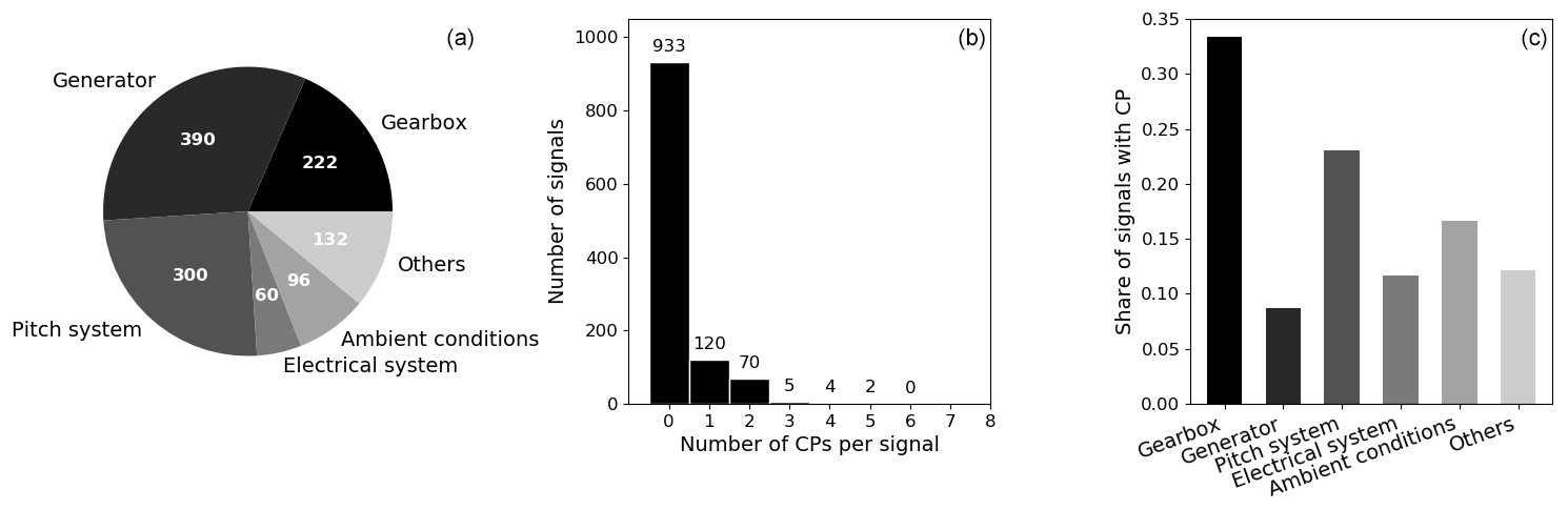
Figure A1 Number of signals per component (a), number of CPs per signal (b), and share of signals with CPs per component (c) for the 1-year time horizon.

Appendix B: List of analysed signals

Table B1 Full list of analysed signals.

Appendix C: Detailed results per component

Figure C1 The 2-year signal validation: F1 scores per component for different hyperparameter configurations and penalty values.

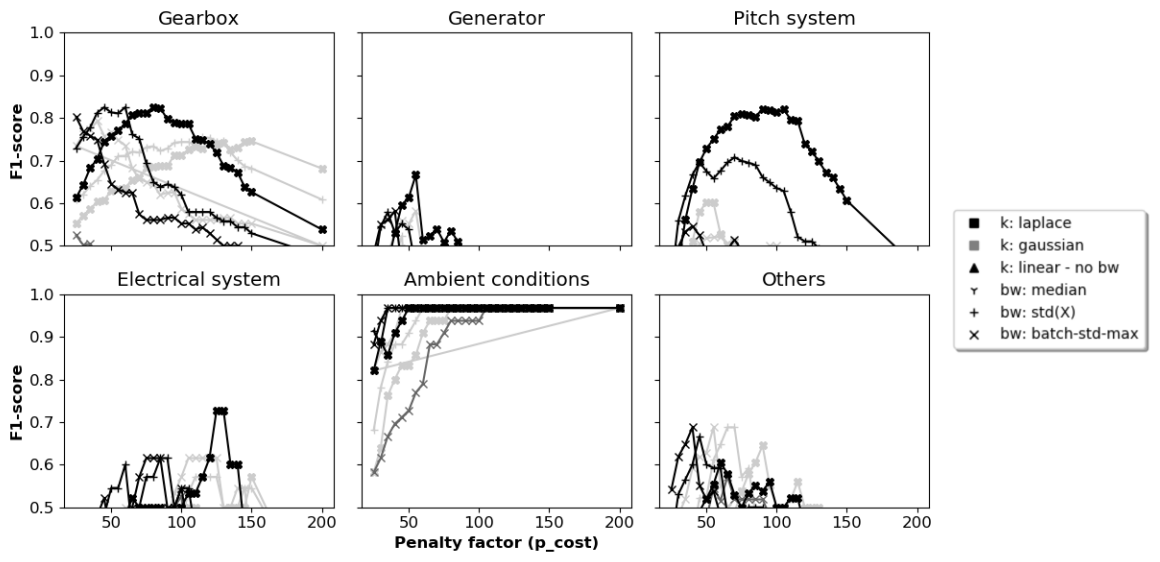
Figure C2 The 1-year signal validation: F1 scores per component for different hyperparameter configurations and penalty values.

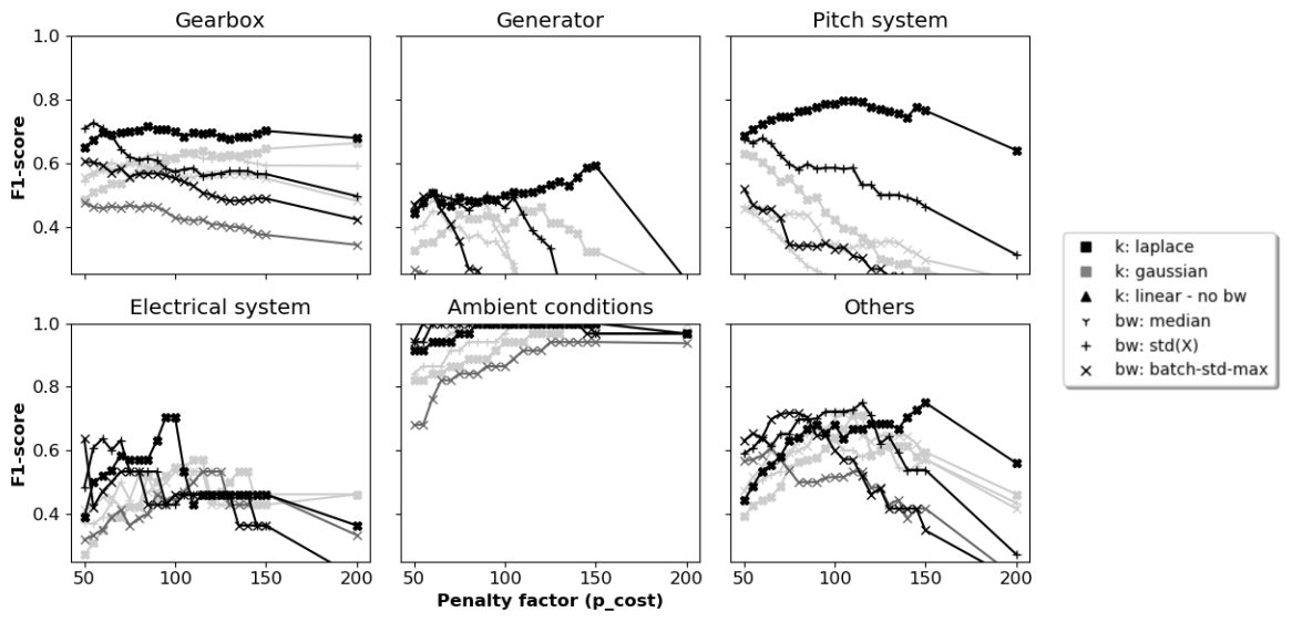
Figure C3 The 2-year signal selection: F1 scores per component for different hyperparameter configurations and penalty values.

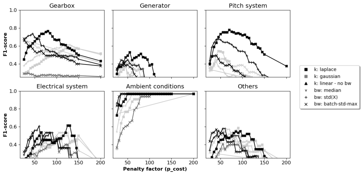
Figure C4 The 1-year signal selection: F1 scores per component for different hyperparameter configurations and penalty values.

Table C1 Results validation per component for best configuration (Laplace/SD-max/α_cost=80) on 1-year signals.

Table C2 Results selection per component for best configuration (Laplace/SD-max/α_cost=80) on 1-year signals.

Appendix D: Results of algorithm without preprocessing

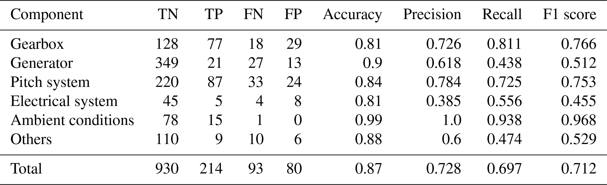
Table D1 Performance of the algorithm without preprocessing on 2-year signals.