the Creative Commons Attribution 4.0 License.
the Creative Commons Attribution 4.0 License.
 | 15 Jun 2020
Is the Blade Element Momentum theory overestimating wind turbine loads? – An aeroelastic comparison between OpenFAST's AeroDyn and QBlade's Lifting-Line Free Vortex Wake method
Sebastian Perez-Becker
Francesco Papi
Joseph Saverin
David Marten
Alessandro Bianchini
Christian Oliver Paschereit
Load calculations play a key role in determining the design loads of different wind turbine components. To obtain the aerodynamic loads for these calculations, the industry relies heavily on the Blade Element Momentum (BEM) theory. BEM methods use several engineering correction models to capture the aerodynamic phenomena present in Design Load Cases (DLCs) with turbulent wind. Because of this, BEM methods can overestimate aerodynamic loads under challenging conditions when compared to higher-order aerodynamic methods – such as the Lifting-Line Free Vortex Wake (LLFVW) method – leading to unnecessarily high design loads and component costs. In this paper, we give a quantitative answer to the question of load overestimation of a particular BEM implementation by comparing the results of aeroelastic load calculations done with the BEM-based OpenFAST code and the QBlade code, which uses a particular implementation of the LLFVW method. We compare extreme and fatigue load predictions from both codes using sixty-six 10 min load simulations of the Danish Technical University (DTU) 10 MW Reference Wind Turbine according to the IEC 61400-1 power production DLC group.
Results from both codes show differences in fatigue and extreme load estimations for the considered sensors of the turbine. LLFVW simulations predict 9 % lower lifetime damage equivalent loads (DELs) for the out-of-plane blade root and the tower base fore–aft bending moments compared to BEM simulations. The results also show that lifetime DELs for the yaw-bearing tilt and yaw moments are 3 % and 4 % lower when calculated with the LLFVW code. An ultimate state analysis shows that extreme loads of the blade root out-of-plane bending moment predicted by the LLFVW simulations are 3 % lower than the moments predicted by BEM simulations. For the maximum tower base fore–aft bending moment, the LLFVW simulations predict an increase of 2 %. Further analysis reveals that there are two main contributors to these load differences. The first is the different way both codes treat the effect of the nonuniform wind field on the local blade aerodynamics. The second is the higher average aerodynamic torque in the LLFVW simulations. It influences the transition between operating modes of the controller and changes the aeroelastic behavior of the turbine, thus affecting the loads.
- Article
(6586 KB) - Full-text XML
- BibTeX
- EndNote


Load calculations are an essential process when designing large modern wind turbines. With the help of such simulations, turbine designers are able to derive the design loads for each of the turbine's components. International guidelines and standards prescribe a large number of aeroelastic simulations of the complete turbine for each load calculation loop (IEC 61400-1 Ed. 3, 2005). These simulations, or Design Load Cases (DLCs), are required in order to cover many possible situations that the wind turbine might encounter in its lifetime and hence calculate realistic loads. In the case of turbulent wind simulations, several repetitions of individual DLCs with different wind realizations are required to limit the effect of statistical outliers and obtain converged results. The current industry trend is to design ever larger wind turbines with increasingly long and slender blades. As the wind turbines become larger, the design loads of each component scale following a power law of the rotor diameter (Jamieson, 2018, 97–123). This leads to increased material requirements and ultimately to higher component costs. Given this fact, there is a large incentive to calculate the components' loads as accurately as possible. If overly conservative load estimates on these large multi-megawatt scales can be avoided, it would result in a considerable reduction in material use and consequently component costs.
Current aeroelastic codes rely mostly on the Blade Element Momentum (BEM) aerodynamic model (Hansen, 2008, 45–55; Burton et al., 2011, 57–66) to calculate aerodynamic loads. BEM models are computationally inexpensive and require a series of engineering corrections to model the more challenging unsteady aerodynamic phenomena usually present in the DLCs. These correction models have been developed and tested so that they work for a wide range of operating conditions. If the turbine happens to operate outside these conditions, BEM methods can introduce inaccuracies in the predicted blade loads and consequently in the turbine design loads. Examples of this include extreme yawed inflow conditions and turbine operation with inhomogeneous induction across the rotor. The latter condition can arise from the turbine operating partially in the wake of another turbine, sheared inflow, turbulent inflow or a large difference in the individual pitch angles of the blades (i.e., pitch faults) (Madsen et al., 2012; Hauptmann et al., 2014; Boorsma et al., 2016). The advantages of BEM methods have become less compelling because of the increase in available computational power. For the same reason, methods with higher-order representations of unsteady aerodynamics have become more attractive. Vortex methods such as the Lifting-Line Free Vortex Wake (LLFVW) aerodynamic model are able to model the turbine wake and its interaction with the turbine directly instead of relying on momentum balance equations – as BEM models do. Therefore, LLFVW models are able to calculate unsteady aerodynamics with far fewer assumptions than BEM models (Hauptmann et al., 2014; Perez-Becker et al., 2018). Using more accurate aerodynamic methods lowers model uncertainty, potentially removing the need for overly conservative safety factors. This would lower design loads, either directly through more accurate load predictions or indirectly through lower safety factors, ultimately leading to more competitive turbine designs.
Over the past years, there have been several studies comparing BEM models with higher-order vortex models. Madsen et al. (2012) compare the predictions of several BEM-based codes, vortex-based codes and computational fluid dynamics (CFD)-based codes. They find, under uniform conditions, that the considered codes predict similar power and thrust. This changes when sheared inflow conditions are simulated. Here, the differences in the predicted power, thrust and load variation between the codes are larger. In Qiu et al. (2014), the authors present a LLFVW method and analyze the unsteady aerodynamic loads in yawing and pitching procedures. Marten et al. (2015) use the LLFVW method implemented in the aeroelastic code QBlade (Marten et al., 2013b, a) to simulate the MEXICO (Snel et al., 2009) and NREL Phase IV (Simms et al., 2001) experiments. They compare the results to experimental data and to predictions from other BEM and vortex codes, showing good agreement with the experimental results.
Several authors have also done aeroelastic comparative studies. Voutsinas et al. (2011) analyze the aeroelastic effect of sweeping a turbine blade backwards. For the NREL/UPWIND 5 MW Reference Wind Turbine (RWT) (Jonkman et al., 2009), they compare the loads predicted with a BEM method and GENUVP – a lifting surface method coupled with a vortex particle representation of the wake (Voutsinas, 2006). Jeong et al. (2014) extended the study from Madsen et al. (2012) by considering flexibility in their turbine model and inflow conditions with turbulent wind. They find that for lower wind speeds (i.e., optimal tip speed ratios and higher), there are noticeable differences in the predicted loads from BEM and LLFVW methods. However, for higher wind speeds (i.e., low tip speed ratios), these differences decrease due to the overall smaller axial induction factors.
Other comparisons of vortex and BEM methods are done in Hauptmann et al. (2014) and Boorsma et al. (2016). Here, the authors compare the aeroelastic predictions of LLFVW and BEM methods for several load cases. Both studies conclude that for their considered cases the LLFVW method predicts lower load fluctuations. Chen et al. (2018) performed a study of the NREL 5 MW RWT considering yawed and shared inflow using a free wake lifting surface model and a geometrically exact beam model. Saverin et al. (2016a) couple the LLFVW method from QBlade to the structural code of FAST (Jonkman and Buhl, 2005). The authors use the NREL 5 MW RWT and compare the loads predicted by the LLFVW method and AeroDyn – the BEM code used in FAST (Moriarty and Hansen, 2005) – showing significant differences in loading and controller behavior. Large differences can also be seen in Saverin et al. (2016b). Here, Saverin et al. (2016b) combine QBlade's LLFVW method and a structural model with a geometrically exact beam model for the rotor blade. Load case simulations are also performed by Perez-Becker et al. (2018). Here, the authors simulate the DTU 10 MW RWT (Bak et al., 2013) in power production DLCs, as defined in IEC 61400-1 Ed. 3 (2005), including wind shear, yaw error and turbulent inflow conditions. They conclude that for wind speeds above the rated wind, the BEM-based aeroelastic code FAST predicts higher fatigue loading and pitch activity than the LLFVW-based code QBlade.
A hybrid implementation that uses a BEM method for the far wake and a Lifting-Line Vortex method for the near wake is presented in Pirrung et al. (2017). Here, Pirrung et al. (2017) compare the predictions of their hybrid near-wake model to a pure BEM method and the Lifting-Surface Free-Wake method GENUVP. Results from pitch step responses and prescribed vibration cases for the NREL 5 MW RWT show that the near-wake method agrees much better with the Lifting-Surface Free-Wake method than with the pure BEM method.
Most of the studies comparing loads have so far focused on specific scenarios, simulating turbines under idealized inflow conditions or using a small number of turbulent load cases. If we wish to quantitatively answer how the results of load calculations differ when we use BEM-based and LLFVW-based methods, we need a large number of turbulent DLCs to level out statistical biases of individual realizations. Many of the mentioned studies also do not include the direct interaction with the turbine controller. Wind turbine load calculations are aero-servo-elastic in nature and the predicted loads are a result of the interaction of the aerodynamics with the turbine structure and controller. Not taking this interaction into account gives an incomplete picture of the effect that different aerodynamic models have on the design loads of the wind turbine.
In this paper, we compare the results of aero-servo-elastic load calculations for the DTU 10 MW RWT. The turbine is simulated according to the IEC 61400-1 Ed.3 DLC groups 1.1 and 1.2 using two different aeroelastic codes: NREL's BEM-based OpenFAST v.2.2.0 (OpenFAST, 2019) and TU Berlin's LLFVW-based QBlade. These DLC groups account for the majority of lifetime fatigue loads of the turbine components. Fatigue and extreme loads of key turbine sensors, derived from sixty-six 10 min simulations covering a wind speed range between 4 and 24 m s−1, are compared and analyzed. Section 2 gives an overview of the aerodynamic and structural codes as well as the controller used in this study. A baseline comparison of the codes under idealized inflow conditions is detailed in Sect. 3, where we compare the performance of our turbine when calculated with both codes. Sections 4 to 6 contain the main contribution of this paper: a comparison and analysis of the results of load calculations with turbulent wind using both codes. Section 4 presents the considered sensors and gives an overview of the results. Section 5 presents, analyses and discusses the fatigue loads. An ultimate load analysis including discussion is presented in Sect. 6, and the conclusions are drawn in Sect. 7.
For this study, we chose to use the DTU 10 MW RWT. It is representative of the new generation of wind turbines and has been used in several research studies. The complete description of the turbine can be found in Bak et al. (2013).
The following subsections briefly present the methods used for aerodynamic and structural modeling, the turbine controller, and the setup used for the load simulations.
2.1 Aerodynamic models
OpenFAST and QBlade are set up so that their only difference is the implemented aerodynamic model. OpenFAST uses AeroDyn – an implementation of the BEM method – and QBlade uses an implementation of the LLFVW method. The following subsections describe the details of these two particular implementations of the BEM and LLFVW methods.
2.1.1 Blade Element Momentum method
The BEM method calculates the aerodynamic loads by combining the Blade Element theory and the Momentum theory of an actuator disc to obtain the induced velocities on every discretized element of the blades (Moriarty and Hansen, 2005). The turbine rotor is divided into independently acting annuli. For each annulus, the thrust and torque obtained from 2-D airfoil polar data of the blade element is equated to the thrust and torque derived from the momentum theory of an actuator disc (Burton et al., 2011, 57–66). This set of equations can be solved iteratively to obtain the forces and moments on each blade element. This theory is only valid for uniformly aligned flows in equilibrium. Several correction models have been developed to extend the BEM method so that more challenging aerodynamic situations can be modeled. The correction models are summarized in Table 1. Details for the implementation of the tip and root loss model, the turbulent wake state model, the oblique inflow model, the dynamic stall model, and the tower shadow model in OpenFAST can be found in Moriarty and Hansen (2005). The other correction models are briefly mentioned below.
-
Wake memory effect. This correction is needed to model the additional time required by the flow to adapt when sudden changes in pitch angle, rotational speed or wind speed occur at the rotor plane. This additional time comes from the interaction of the flow with the rotor wake. OpenFAST recently introduced this feature via the optional Dynamic BEM theory (DBEMT) module. It is the model by Øye presented in Snel and Schepers (1995) that filters the induced velocities via two first-order differential equations.
-
Stall delay. Blade Element theory assumes no interaction between the blade elements. For rotating airfoils in the inner part of a wind turbine blade there is a significant amount of radial flow. This phenomenon delays the effective angle of attack at which the airfoil stalls (when compared to the 2-D airfoil polar data). OpenFAST does not have an explicit model for stall delay. Instead, the airfoil polar data have to be preprocessed using an appropriate model before it is implemented in the code. For this study we used the 3-D-corrected airfoil polar data presented in Bak et al. (2013). The corrected airfoil data were obtained using the method described in Bak et al. (2006).
Table 1Modeling differences of the two aerodynamic codes. I stands for intrinsic, and EM stands for engineering model.

2.1.2 Lifting-Line Free Vortex Wake method
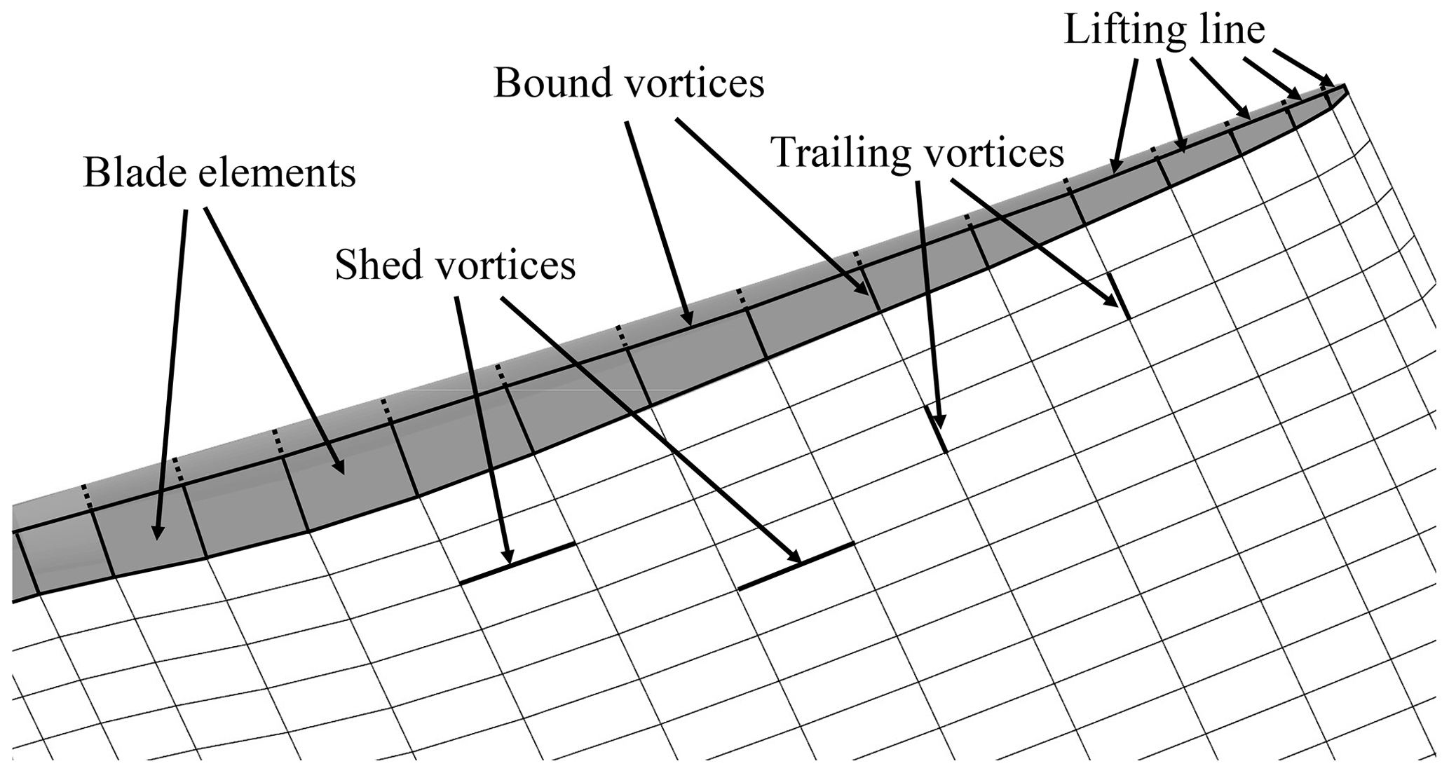
The LLFVW method is based on inviscid potential flow theory and a vortex representation of the flow field (Van Garrel, 2003; Marten et al., 2015). In the implementation found in QBlade, the rotor blade is discretized into elements represented by bound ring vortices. These bound vortices are located at the quarter chord position, and their sum makes up a lifting line. By using the Kutta–Joukowski theorem and the airfoil polar data corresponding to the blade element, we can calculate the circulation of the bound vortices:
In this equation, Γ is the circulation of the blade element, L is the lift per unit length, ρ the density, Vtot the total velocity, Cl the lift coefficient, α the angle of attack and c the local chord. The total velocity is the sum of the incoming velocity V∞, the velocity due to the motion of the blade (rotation/deflection) Vmot and the induced velocity from the wake VΓ:
The induced velocity from all the vortex elements in the wake can be calculated by applying the Biot–Savart Law at each blade element:
Here, xp is the control point where the Biot–Savart Law is evaluated (e.g., the blade element), x is the position of each of the wake vortices and dl their vectorized length.
Equations (1)–(3) can be solved iteratively to obtain the circulation, the induced velocity and the forces at each blade element. At each time step, the circulation is shed to the wake creating trailing and shed vortices. The former arise from the spanwise variation in the circulation and the latter from the temporal variation. By applying Eq. (3) to the wake vortices, the free convection of the wake can be modeled.
In order to avoid a singularity when evaluating Eq. (3) at the vortex centers, the vortex core model proposed by van Garrel was used (Van Garrel, 2003; Marten et al., 2015). The initial vortex core size was set to be 0.3 times the local chord length of the blade element and was used for bound and wake vortices. This initial value was determined based on a preliminary sensitivity study with idealized wind conditions. Figure 1 shows a closeup of a wind turbine blade during a LLFVW simulation using the aero-servo-elastic code QBlade. It includes the concepts explained in this section.
While capturing the flow physics of a wind turbine rotor much more accurately, LLFVW methods still use some correction models to account for all the aerodynamic phenomena present in turbulent load calculations, briefly explained here.
-
Dynamic stall. Because of the potential flow assumption and the use of airfoil polar data, a model is needed to account for the flow separation phenomenon. QBlade's LLFVW method uses the ATEFlap unsteady aerodynamic model (Bergami and Gaunaa, 2012), modified so that it excludes contribution of the wake in the attached flow region (Wendler et al., 2016).
-
Tower shadow. The effect of the tower on the blade aerodynamics also has to be taken into account explicitly in the LLFVW simulations via an engineering model. QBlade uses the same potential flow model that is also used in OpenFAST (Bak et al., 2001).
-
Stall delay. As with the BEM method, the stall delay phenomenon is included via modified airfoil polar data using an appropriate model. We used the same 3-D-corrected airfoil polar data in both codes. The data were obtained with the method described in Bak et al. (2006).
2.1.3 Comparison between the aerodynamic models
Table 1 summarizes the differences between the two aerodynamic models.
The LLFVW method explicitly includes most of the phenomena present in DLC simulations with turbulent wind conditions. Usual DLC configurations include sheared and oblique inflow as well as temporal and spatial variations in the incoming wind speed. Unlike the BEM method that solves for the axial and tangential induction factors at each blade element, the LLFVW method solves for the complete flow around the rotor.
Turbine configurations can have coned blades. Including cone angles, as well as the blade prebend and blade deflections in the case of aeroelastic calculations, violates the assumption made in many BEM methods that the momentum balance takes place in independently acting annuli in the rotor plane. Recently, a BEM method that can model the effect of coned blades and radial induction has been proposed in Madsen et al. (2020). These corrections are not included in other BEM implementations such as AeroDyn. Thus, aerodynamic load predictions for the turbulent load cases obtained from the considered LLFVW method are expected to be more accurate compared to predictions from the considered BEM method. The radial induction mentioned in Table 1 comes from the effect of the trailing vortices in the wake.
2.2 Structural model
The structural model used for this study in both OpenFAST and QBlade is ElastoDyn (Jonkman, 2014). It uses a combined multi-body and modal dynamics representation that is able to model the wind turbine with flexible blades and tower (Jonkman, 2003). The modal representation of blades and tower uses an Euler–Bernoulli beam model to calculate deflections. It also includes corrections to account for geometrical nonlinearities. The structural model allows for four tower modes: the first two fore–aft and side–side modes. As for the blade, three modes are modeled in ElastoDyn: the first and second flapwise modes and the first edgewise mode. The structural model does not take into account shear deformation and axial and torsional degrees of freedom.
Both OpenFAST and QBlade have additional models that allow for a more accurate representation of the wind turbine structural dynamics. The module BeamDyn in OpenFAST is able to model the blade as a geometrically exact beam (Wang et al., 2016), and QBlade has a structural solver based on the open-source multi-physics library CHRONO (Tasora et al., 2016). The latter uses a multi-body representation which includes Euler–Bernoulli beam elements in a co-rotational formulation. More accurate representations of the structural deflection of the wind turbine – in particular blade torsional deflection – have a significant influence on the loads. Torsional deflection changes the local angle of attack of a blade section and hence the lift force. This can lead to very different blade dynamics when compared to a model that does not include this degree of freedom. The torsional degree of freedom also tightens the aero-servo-elastic coupling of the turbine by again changing the local angle of attack of the blade sections. The integrated effect of this directly influences the pitch controller.
Saverin et al. (2016b) compared the results of aero-servo-elastic simulations using three configurations of structural and aerodynamic codes: ElastoDyn coupled with AeroDyn's BEM method, ElastoDyn coupled with QBlade's LLFVW method and BeamDyn coupled with QBlade's LLFVW method. They show that the differences in pitch controller behavior and blade tip deflection are much larger between the BeamDyn–QBlade and the ElastoDyn–QBlade configurations – which differ in the structural code – than the differences between ElastoDyn–AeroDyn and ElastoDyn–QBlade configurations – which differ in the aerodynamic code.
This indicates that the differences in aerodynamic loads from BEM-based and LLFVW-based codes will certainly be more marked when studied in conjunction with a more accurate structural model that allows for the torsional degree of freedom. Nonetheless, we decided to use ElastoDyn as the structural model for our study. It is shared by both aeroelastic codes, so by using it, we keep the modeling differences only in the aerodynamic module and ensure that the latter is the only source of the load differences.
2.3 Controller
To enable aero-servo-elastic studies, we implemented a wind turbine controller that is compatible with both codes. The controller is based on the DTU Wind Energy Controller (Hansen et al., 2013), which features pitch and torque control. It has been extended with a supervisory control based on a report by Iribas et al. (2015). The supervisory control allows the controller to run a full load analysis. The controller parameters were taken from the report (Borg et al., 2015). Only the optimal torque–speed gain was recalculated based on the maximum power coefficient obtained from OpenFAST calculations.
The controller parameters were obtained via BEM calculations, so it is expected that the controller will behave differently if used in LLFVW calculations. In a normal design situation, each controller is tuned to the aeroelastic turbine model in order to optimize for the control objectives (i.e., maximize energy capture and minimize turbine loads). Since the aeroelastic models are inherently different due to the aerodynamic models, the tuning of the controller would result in different parameters depending on the aerodynamic model. We deliberately did not retune the controller parameters for the LLFVW simulations. Since the controller parameters were optimized for BEM simulations, we expect that the energy capture or the load level (or even both) will not be optimal in the LLFVW simulations. By doing this though, we ensure that the load differences arise only from the different aerodynamic models themselves and their interaction with identical turbine controllers. With the structural models also being identical, we can clearly attribute the load differences to the aerodynamic models.
2.4 Practical considerations for load calculations
In order to use the presented methods in load calculations, several practical considerations had to be taken into account. Given that Eq. (3) has to be evaluated for each vortex element in the wake, calculating the convection of the wake can be computationally costly, slowing down the LLFVW calculations. In order to increase the calculation speed of these simulations, we implemented two wake-coarsening methods. The first one follows a similar method as the one described in Boorsma et al. (2018). Instead of skipping or removing vortices, the method implemented in QBlade lumps the wake elements together after a given number of rotor revolutions. The method reduces the number of vortex elements in the wake while conserving the total vorticity. This is done in two stages, giving us three wake regions: the near wake, the mid-wake and the far wake. The number of vortices lumped together is given by a lumping factor. Thus, QBlade uses two lumping factors: the mid-wake factor for the transition from near wake to mid-wake and the far-wake factor for the transition from mid-wake to far wake.
The second method is the wake cutoff. After a given amount of rotor revolutions, the wake is cut off. The influence of these far-wake vortex elements on the velocity in the rotor plane is negligible. Removing these elements helps speeding up the calculations. Figure 2 shows the combination of the two implemented wake-coarsening methods. The wake-coarsening methods are a function of rotor revolutions. Because the effect of the vortex elements on the induced velocity is a function of the distance, the parameters for these methods will be dependent on the wind speed. The latter has an impact on the rotor speed and on the convection speed of the vortex elements. The wake-coarsening parameters that we used for our simulations are given in Table A1.
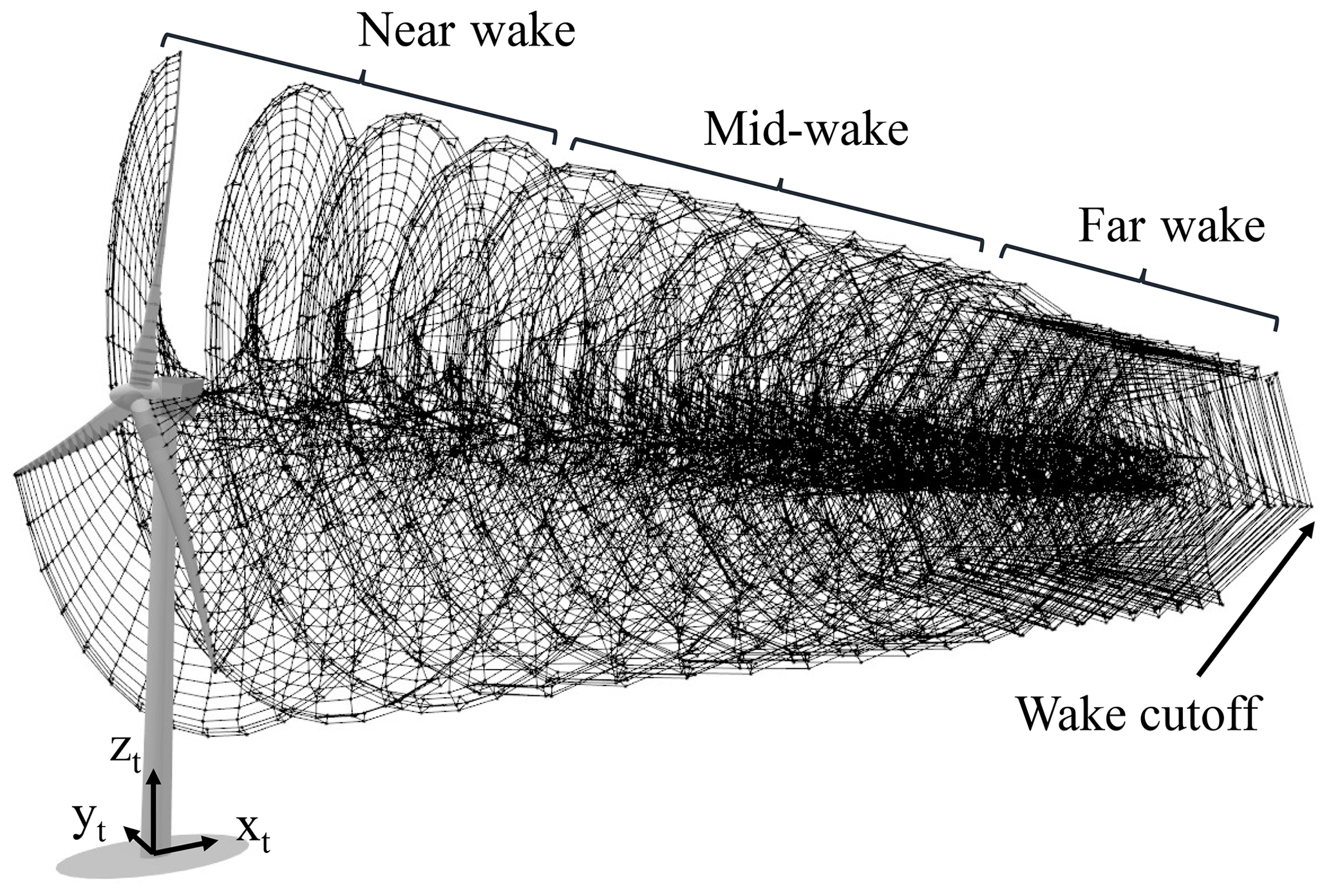
Figure 2Wake-coarsening methods for the LLFVW simulations: the wake is split into three regions with decreasing amounts of wake elements. After a given number of revolutions, the wake is cut off.
Table 2Simulation parameters for aerodynamic and aeroelastic simulations.

To do a baseline comparison of our aerodynamic models, we ran a series of idealized aerodynamic simulations. The parameters for these simulations are summarized in Table 2 under the column “Aerodynamic calculations”. With these settings the flow is axis-symmetric on the rotor and no elasticity is taken into account. Under these conditions, many of the engineering correction models do not affect the rotor aerodynamics. Table 1 shows that the only BEM engineering correction models that affect the rotor aerodynamics under these conditions are the tip and root loss model and the turbulent wake state for high tip speed ratios (i.e., low wind speeds).
Figure 3 shows the steady-state performance coefficients for aerodynamic calculations when done with the BEM and LLFVW codes. In general, the performance coefficients from both calculations agree well. The thrust coefficient from LLFVW calculations follows the thrust coefficient from BEM calculations very closely (Fig. 3a). It is only at a wind speed of 11 m s−1 that the values visibly differ. As for the power coefficient (Fig. 3b), the LLFVW code predicts higher values for wind speeds below the rated wind speed. Above the rated wind speed, the power coefficients in both codes almost perfectly match. This behavior can be explained by the fact that at higher wind speeds the turbine controller pitches the blades out to keep the power output of the turbine constant. The controller logic is identical in both codes. Additionally, at higher wind speeds the rotor speed is kept constant by the controller while the convection speed of the wake increases. This decreases the influence of the wake on the turbine's thrust and power and hence the differences in the aerodynamic models become smaller. If we compare numerical values at 8 m s−1, the difference between the thrust and power coefficients from both codes is 1.1 % and 4.6 %, respectively. Similar differences of power and thrust between BEM and LLFVW codes for 8 m s−1 and ideal inflow conditions were also reported in Madsen et al. (2012).
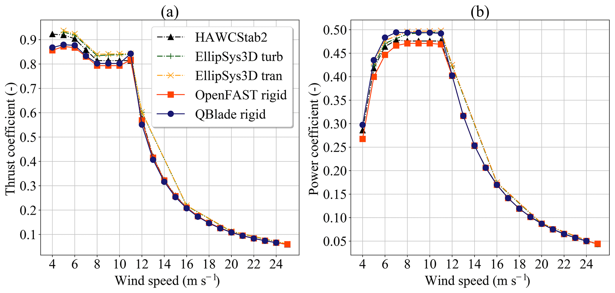
Figure 3Performance coefficients for aerodynamic simulations with idealized conditions: (a) thrust coefficient and (b) power coefficient.
Figure 3 also contains data from three calculations done with other codes. The data are taken from Bak et al. (2013), where the performance coefficients of the rigid DTU 10 MW RWT are calculated with the BEM-based code HAWCStab2 and the CFD-based code EllipSys3D. For the latter, two different boundary layer models were used. The OpenFAST and HAWCStab2 calculations predict very similar performance coefficients except for low wind speeds. QBlade predicts thrust coefficients that are closer to the BEM-based codes and power coefficients that are closer to the CFD-based codes.
The turbulent load calculations described in Sect. 4 used the full aeroelastic turbine model. The simulation parameters for the full aeroelastic model are summarized in Table 2 under the column “Aeroelastic calculations”. Because of the long simulation time of each load case, we applied more aggressive wake-coarsening parameters for the aeroelastic calculations than for the aerodynamic calculations. These are also summarized in Table A1. These simulation parameters are the result of a sensitivity study we performed to make sure that our chosen wind-dependent wake parameters for the aeroelastic LLFVW simulations predicted similar steady-state values compared to the idealized aerodynamic calculations with long wakes.
Figure 4 shows the comparison of the rotor thrust, rotor power, pitch angle and rotor speed for the aerodynamic and aeroelastic calculations. Using the parameters from the column “Sensitivity study” in Table 2 only has a small influence on the steady-state values of the rotor thrust and power (Fig. 4a and b). For both OpenFAST and QBlade, the rotor thrust from aeroelastic calculations is slightly higher that the thrust from purely aerodynamic calculations (as defined in column “Aerodynamic calculations” from Table 2). For the wind speeds between 9 and 12 m s−1, the difference in thrust between aeroelastic and aerodynamic calculations in QBlade is more marked than the difference in OpenFAST.

Figure 4Comparison of aerodynamic and aeroelastic calculations on turbine performance: (a) rotor thrust, (b) rotor power, (c) pitch angle and (d) rotor speed.
The rotor speeds and pitch angles for the aerodynamic and aeroelastic calculations are shown in Fig. 4c and d, respectively. In these subfigures we can see that there is also little difference in the controller signals if the turbine is simulated aeroelastically. The pitch angle coincides for all simulations. The reason for this probably comes from the fact that the structural model does not include the blade torsional degree of freedom. As for the rotor speed, QBlade predicts higher rotor speeds than OpenFAST for wind speeds between 7 and 11 m s−1. Particularly for 11 m s−1 wind speed, QBlade simulations already reach the rated rotor speed, while OpenFAST predicts a steady-state rotor speed of 0.953 rad s−1. This fact explains the higher thrust (Fig. 4a) and thrust coefficient (Fig. 3a) for this wind speed.
The higher rotor speeds obtained in QBlade simulations at those wind speeds can be explained from the higher power coefficients seen in Fig. 3b. Given the fact that the aerodynamic loads are calculated with inherently different models, it is to be expected that there will be some differences in the induction factors and hence in the tangential blade loads.
An important result from Fig. 4 is that using the wake-coarsening parameters from Table A1 has only a small effect on the accuracy of the aeroelastic steady-state results compared to the aerodynamic results. Therefore, the coarsening parameters can be used to speed up the turbulent load calculations in the next section.
The turbulent wind load cases were calculated following the DLC groups 1.1/1.2 from the IEC61400-1 standard (IEC 61400-1 Ed. 3, 2005). These DLC groups refer to the normal power production simulations of the turbine. For onshore wind turbines, the DLC group 1.2 is the main contributor of lifetime fatigue loads for most of the turbine components, since the turbine spends most of the operating time in these conditions. Evaluating the fatigue loads from this group will therefore give a close estimate of the real fatigue loads while keeping the number of simulations relatively low. The turbine setup for these load cases is listed in Table 2 in the third column. In this study, we considered wind speed bins (defined by the mean VHub) between 4 to 24 m s−1 in 2 m s−1 steps. For each wind speed bin, six simulations were performed using two turbulence seeds per yaw angle. The same wind fields were used for BEM and LLFVW calculations. In total we did 66 simulations with 600 s simulation time for both the BEM and LLFVW codes. To give time for the wake to develop in the LLFVW calculations, we included an extra 100 s simulation time that was discarded in the load analysis. These discarded 100 s wake build-up times were also included in the BEM-simulations to make sure that we had the same incoming wind conditions for both codes.
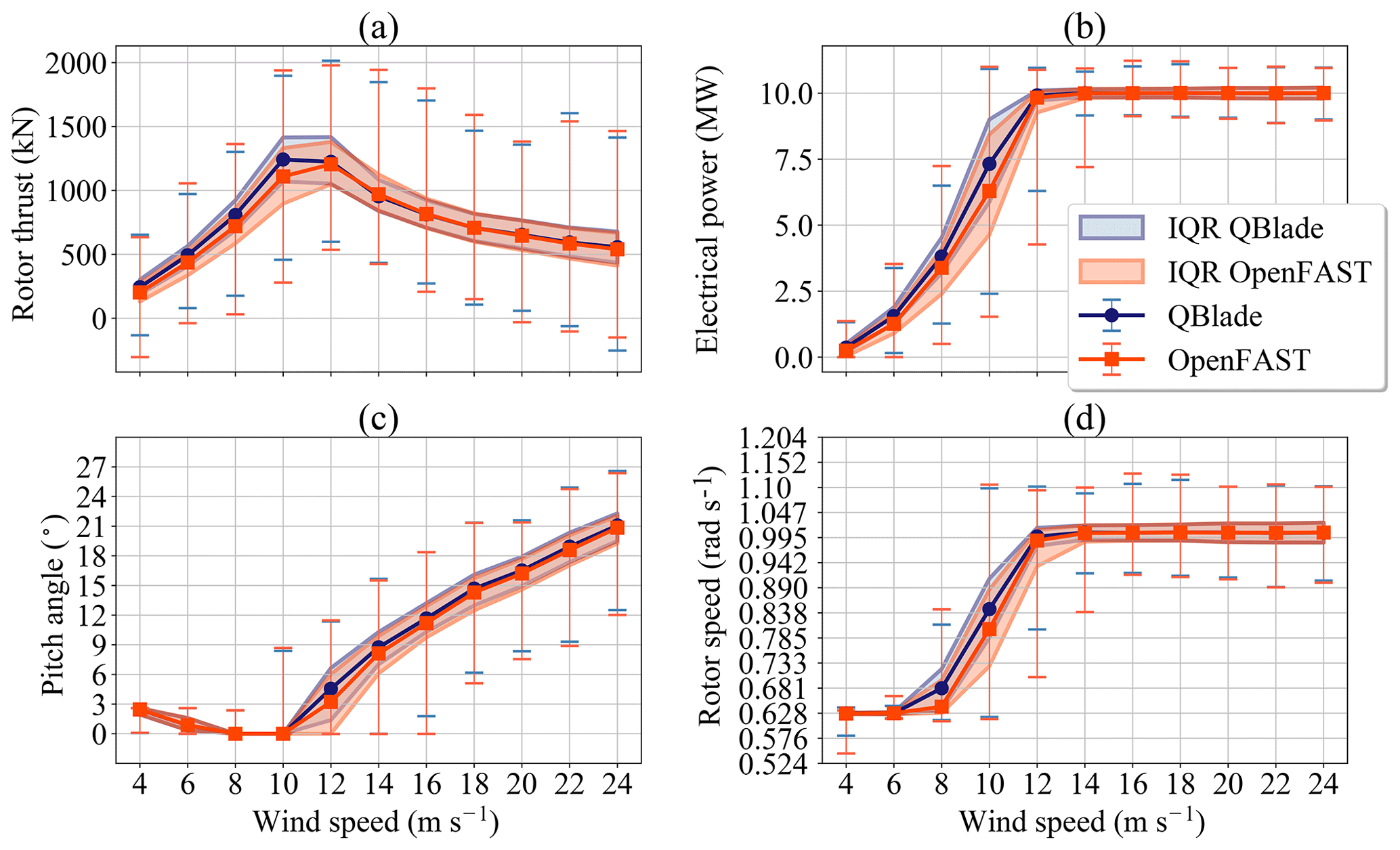
Figure 5Comparison of statistical values for turbulent calculations: (a) rotor thrust, (b) electrical power, (c) pitch angle and (d) rotor speed. IQR stands for interquartile range.
4.1 Considered sensors
For the analysis of the turbulent wind load calculations, we considered a selection of load sensors that is representative of the dynamics and load level of the entire turbine. For the blade analysis, we included the blade root in-plane and out-of-plane bending moments and the blade tip in-plane and out-of-plane deflections. These sensors give a good overview of the overall blade dynamics. The in-plane quantities are mainly driven by gravity loads. Our focus is more on the out-of-plane quantities that are mostly driven by the aerodynamic loads. Differences in the aerodynamic models will have the highest impact on these latter quantities. We also included the yaw-bearing roll, tilt, and yaw moments and the tower top fore–aft and side–side deflections. These sensors characterize the tower top loads and dynamics. All of these sensors, with the exception of the tower top side–side deflection, are directly affected by the aerodynamic loads. Finally we included the tower base fore–aft, side–side and torsional bending moment as indicators of the tower loads. Here, our focus is on the tower base fore–aft bending moment, as it is the sensor most affected by the aerodynamic loads. To analyze if the different aerodynamic models also affect the controller behavior, we included the collective pitch angle and the rotor speed in our analysis.
Table 3 lists all considered sensors for this study and their corresponding symbol. For each sensor group, we used the coordinate systems defined in Jonkman and Buhl (2005) for both OpenFAST and QBlade calculations. The coordinate systems are listed in Table 3. In addition, the table also lists the type of post-processing analysis that we performed for each sensor group. F stands for fatigue load analysis and U for ultimate load analysis. Figure 2 exemplarily shows the tower base coordinate system t.
Table 3Considered sensors and analysis type for turbulent load calculations. CS stands for coordinate system, F stands for fatigue and U stands for ultimate.
4.2 Statistical overview
Figure 5 shows an overview of the statistical values of rotor thrust, electrical power, pitch angle and rotor speed for the turbulent wind calculations of both codes. The markers joined with lines represent the median of all values of the six 600 s simulations in each wind bin. The shaded area represents the interquartile range (IQR) of the time series data – the range in which 50 % of the simulation values of each wind speed bin lie. The error bars represent the extrema of all values recorded at one wind speed bin.
As a general observation, we can see that statistical values for the shown sensors are similar in both codes. There are some differences though.
Let us consider the rotor thrust in Fig. 5a first. We can see that for wind speeds lower than the rated wind speed the values of the rotor thrust calculated with the LLFVW code tend to be higher than the values from the BEM code. This tendency is no longer seen for wind speeds of 12 m s−1 and above. Here the medians and IQRs between both codes almost match. This behavior of the thrust as a function of the wind speed is also seen for the steady-state values in Fig. 4a.
The comparison of electrical power from the turbulent wind simulations (Fig. 5b) also shows similarities with the comparison in ideal situations (Fig. 4b). For the below rated wind speeds, the LLFVW simulations show higher medians of the electrical power than results from BEM simulations. In contrast, the IQRs are lower for the LLFVW simulations. For the 12 m s−1 wind speed bin, the median electrical power for the LLFVW calculation is already practically 10 MW, while the median power of the BEM simulations is still 9.8 MW. Also, we can see from the IQRs that at 12 m s−1 wind speed a higher percentage of time the power from BEM simulations lies below the rated power.
The rotor speed signal (Fig. 5d) is closely linked to the power signal (Fig. 5b). Most observations made for the electrical power also hold true for the rotor speed. The exception being the IQRs of the signal for the 8 m s−1 wind bin. Here the IQR of the rotor speed is smaller in the BEM simulations than in the LLFVW simulations.
Finally, Fig. 5c shows a comparison of the pitch angles between both codes. For wind speeds between 4 and 8 m s−1, there is practically no difference between the statistical values from the BEM and the LLFVW simulations. For higher wind speeds, we can see that the LLFVW simulations have slightly higher median, first quartile and third quartile values than BEM simulations. This behavior was not seen in the idealized aeroelastic simulations (Fig. 4c) where the steady-state values of the pitch angles where almost identical.
While the median values of the sensors shown in Fig. 5 follow the behavior of the steady loads in Fig. 4, differences in the IQRs reveal that the variability of the signals changes if we use different aerodynamic models. Higher IQRs of rotor thrust in the BEM simulations for wind speed bins of 8 and 10 m s−1 seen in Fig. 5a indicate that the fatigue loads of the out-of-plane load sensors in these simulations will be higher.
As for the other three sensors, we see that (particularly for the wind speeds between 8 and 14 m s−1) the IQR of the pitch angle, the rotor speed and the electrical power from the BEM calculations is visibly larger than the IQR of these signals from the LLFVW calculations. These three sensors all represent controller signals. Thus, we can already see that the different aerodynamic models affect the controller behavior even when the controllers are identical. Higher variation in controller signals in the BEM simulations is another indicator that the overall turbine loads will be higher for these simulations.
It is clear that the aerodynamic models have an influence on the overall turbine behavior and loads. However, the mechanisms of how these models affect the loads are not straightforward. In the subsequent sections a quantitative analysis and discussion of these effects is presented.
In this section, we discuss the influence of the aerodynamic models on the variability of controller signals and fatigue loads of different turbine sensors. The analysis is based on the results of the turbulent load calculations described in the previous section. In this and the following sections, the subscripts (⋅)BEM and (⋅)LLFVW denote values obtained from BEM and LLFVW simulations, respectively.
5.1 Controller signals
To quantify the variability of the control signals, we used the standard deviation σ(⋅) as our metric. For each of the six simulations in one wind speed bin, we calculate σ for the rotor speed Ω and the pitch angle θ. We then average all 6 standard deviations for each control signal to get a representative quantity for the signal's variability for that wind speed bin. These averaged standard deviations are denoted as for the pitch angle and for the rotor speed.
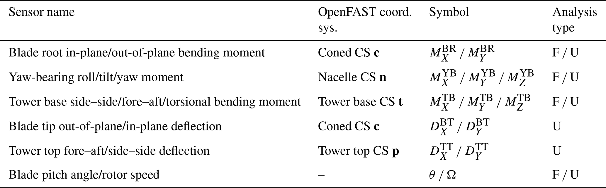
Figure 6 shows the normalized and for all of the simulated wind speed bins. The normalization is with respect to the values from the BEM simulations, so the normalized and are always 1.
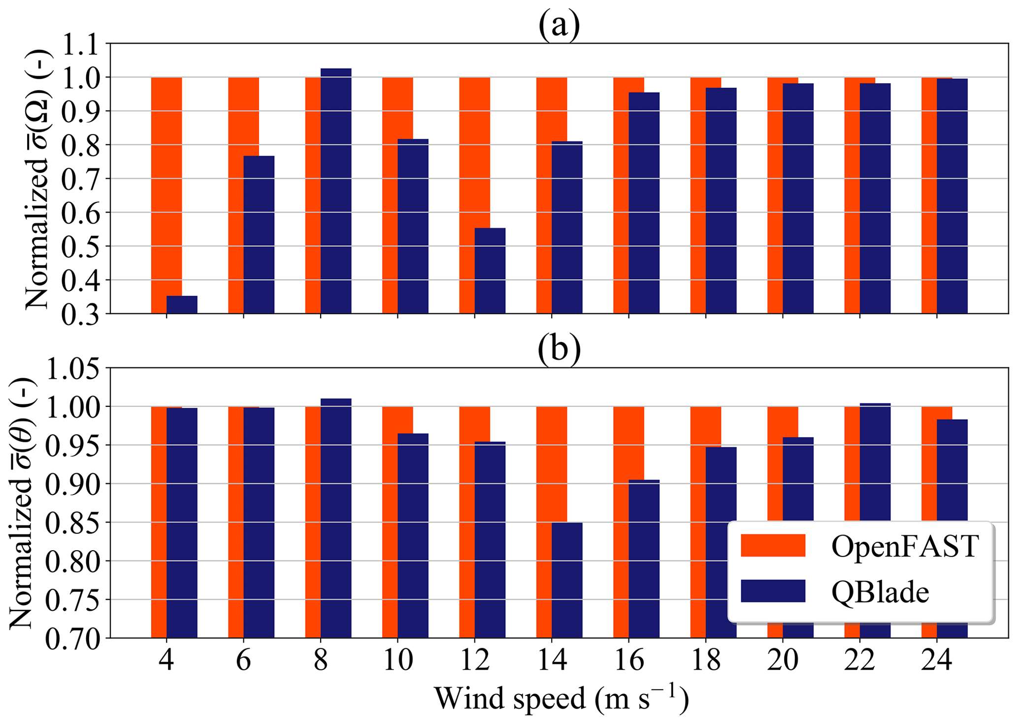
Figure 6Normalized averaged standard deviations vs. wind speed: (a) rotor speed Ω and (b) pitch angle θ.
If we consider the rotor speed (Fig. 6a), we see that for all wind speed bins except 8 m s−1, the normalized is lower than 1. The largest deviations can be seen at wind speed bins of 4 and 12 m s−1. Here, the normalized are 0.35 and 0.55. When we consider wind speed bins of 16 m s−1 and above, we see the normalized value of increase monotonically towards 1.
Why do we have these differences in the wind speed bins 4 and 12 m s−1? In the case of the 4 m s−1 wind bin, this difference can be explained if we look at Fig. 5d. For very low wind speeds, the value of Ω is almost always Ωmin (the minimum rotor speed). However, in the BEM simulations, there are load cases where ΩBEM drops below Ωmin and reaches a lower value than ΩLLFVW. Because of the small absolute value of at those wind speeds, those excursions of ΩBEM have a higher relative effect on and also on the normalized .
As for at the wind speed bin of 12 m s−1, the large difference comes from the fact that the LLFVW simulations predicted higher aerodynamic torque and hence higher values of ΩLLFVW compared to ΩBEM at below-rated wind speed. For example, ΩLLFVW is already ΩR (rated rotor speed) at wind speed 11 m s−1 in Fig. 4d, while ΩBEM is slightly above 0.94 rad s−1. For turbulent calculations, the variation in ΩLLFVW in Fig. 5d is smaller than the variation in ΩBEM mainly because the turbine has reached ΩR at more time instants in the LLFVW simulations and the pitch controller is keeping the power and rotor speed constant.
For the pitch angle signal we can see that the normalized behaves differently as a function of wind speed than , while generally having values below 1 (Fig. 6b). For wind speed bins between 10 and 16 m s−1, drops to values significantly lower than 1, reaching a value of 0.85 for the 14 m s−1 wind speed bin. For low wind speed bins, is practically 1. For the wind speed bins of 18 m s−1 and above, the normalized values of are above 0.95.
5.2 Loads
The fatigue loads are quantified using the damage equivalent loads (DELs) metric. DELs are derived from the time series of the load sensor using a rain flow counting algorithm. In this algorithm, the time-varying signal is broken down into individual cycles by matching local minima and maxima in the time series (Hayman, 2012). The rain flow counting was performed using NREL's post-processing software Crunch (Buhl, 2018). We used the Palmgren–Miner linear damage accumulation hypothesis to obtain the DELs. Two types of fatigue loads were calculated. The first type are the short-term 1 Hz DELs – denoted as DEL1 Hz(⋅) – which give us the equivalent fatigue damage of one simulation. The second type are the lifetime DELs – denoted as DELLife(⋅) – which give us the equivalent loading for the entire turbine lifetime. The lifetime DELs were obtained following the method described in Hayman (2012). We used the wind distribution corresponding to wind class IA turbine with a 20-year design life and an equivalent cycle number of 107. For the blade root fatigue loads, we used an inverse S–N curve-slope of m=10 to calculate the DELs. For all other loads, the inverse S–N curve-slope used is m=4.
Figure 7 shows the normalized lifetime DELs for the considered turbine load sensors. We can see from this figure that performing the simulations with different aerodynamic models has an impact on the lifetime DELs of almost all considered load sensors. Let us start with the blade root. For these loads we see that the normalized DEL and DEL are 0.98 and 0.89, respectively. The finding that the fatigue loads of are lower than has also been reported by other studies, e.g., Perez-Becker et al. (2018) and Boorsma et al. (2016). The studies report normalized values of DEL between 1.006 and 0.77 for turbulent wind simulations, depending on the wind speed. It should be noted that previous studies considered one simulation per wind speed and less time per simulation. This makes a direct comparison of lifetime fatigue loading with the cited literature difficult. However, the results agree qualitatively.
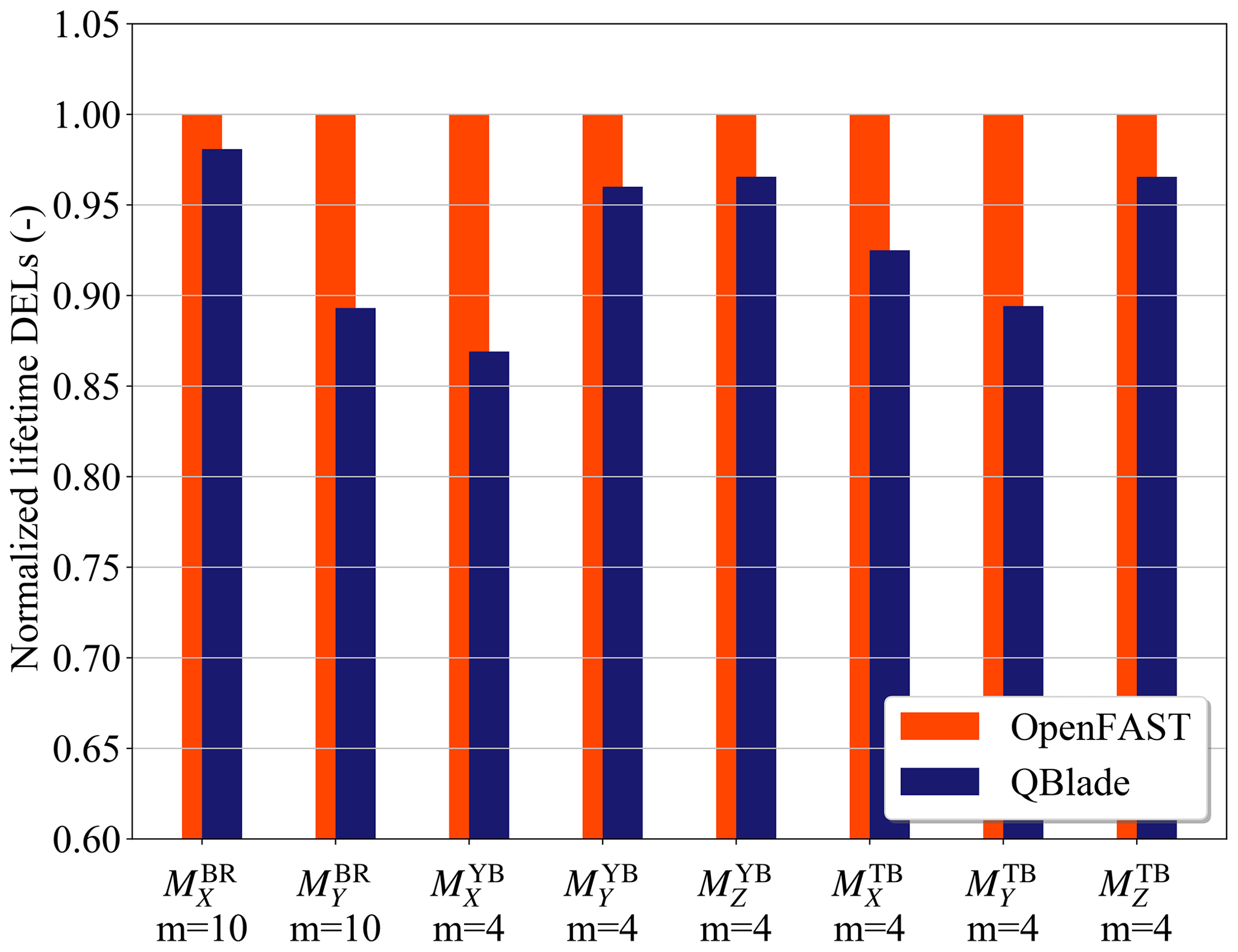
Figure 7Normalized lifetime DELs for the considered turbine load sensors. Sensor notation is given in Table 3.
When considering the yaw bearing, Fig. 7 shows that the normalized DEL has an even lower value than the blade root fatigue loads: 0.87. If we look at the other bending moments, we see a smaller difference between the LLFVW and BEM codes. The normalized values of DEL and DEL are 0.96 and 0.97, respectively. For the tower loads, the largest difference in the lifetime DELs occurs in the tower base fore–aft bending moment. The normalized value of DEL is 0.89. The normalized values of DEL and DEL are 0.92 and 0.97.
Figure 8Normalized averaged 1 Hz DEL as a function of the wind speed bin: (a) blade root out-of-plane bending moment , (b) yaw-bearing roll moment , (c) tower base fore–aft bending moment and (d) yaw-bearing tilt moment .
When calculating the lifetime fatigue loads, we take into account the loading of all the wind speed bins. In different wind speed bins, the turbine can see qualitatively different loading scenarios leading to significant differences in fatigue loading when simulated with different aerodynamic models. To further understand which phenomena are contributing to the differences in fatigue loads, we also analyzed the contribution of the individual wind speed bins to the fatigue loading of the sensors. As we can see in Fig. 8, the contribution of the wind speed bins to the lifetime fatigue loads is strongly dependent on the wind speed. To limit the extent of the fatigue analysis, we will concentrate on four load sensors: , , and .
Figure 8a shows the normalized average 1 Hz DEL for as a function of the wind speed bin. The average, denoted as , was taken from the 1 Hz DELs of each of the six realizations in one wind speed bin. The normalization was done with respect to the values of the BEM simulations. We can see in this subfigure that the value of the normalized is lower than 1 for all wind speed bins except 4 m s−1. For the rest of the wind speed bins, takes values around 0.9.
A different behavior can be seen for the sensor in Fig. 8c, where increase from about 0.7 to just over 0.9 with increasing wind speed. After rated wind speed, remains fairly constant.
The behavior of the fatigue damage on the yaw-bearing sensors is also qualitatively different from the tower base fore–aft and the blade root out-of-plane bending moments. Figure 8b and d show the values of and for all the simulated wind speed bins. For these sensors, the highest differences are seen in wind speed bins between 8 and 12 m s−1.
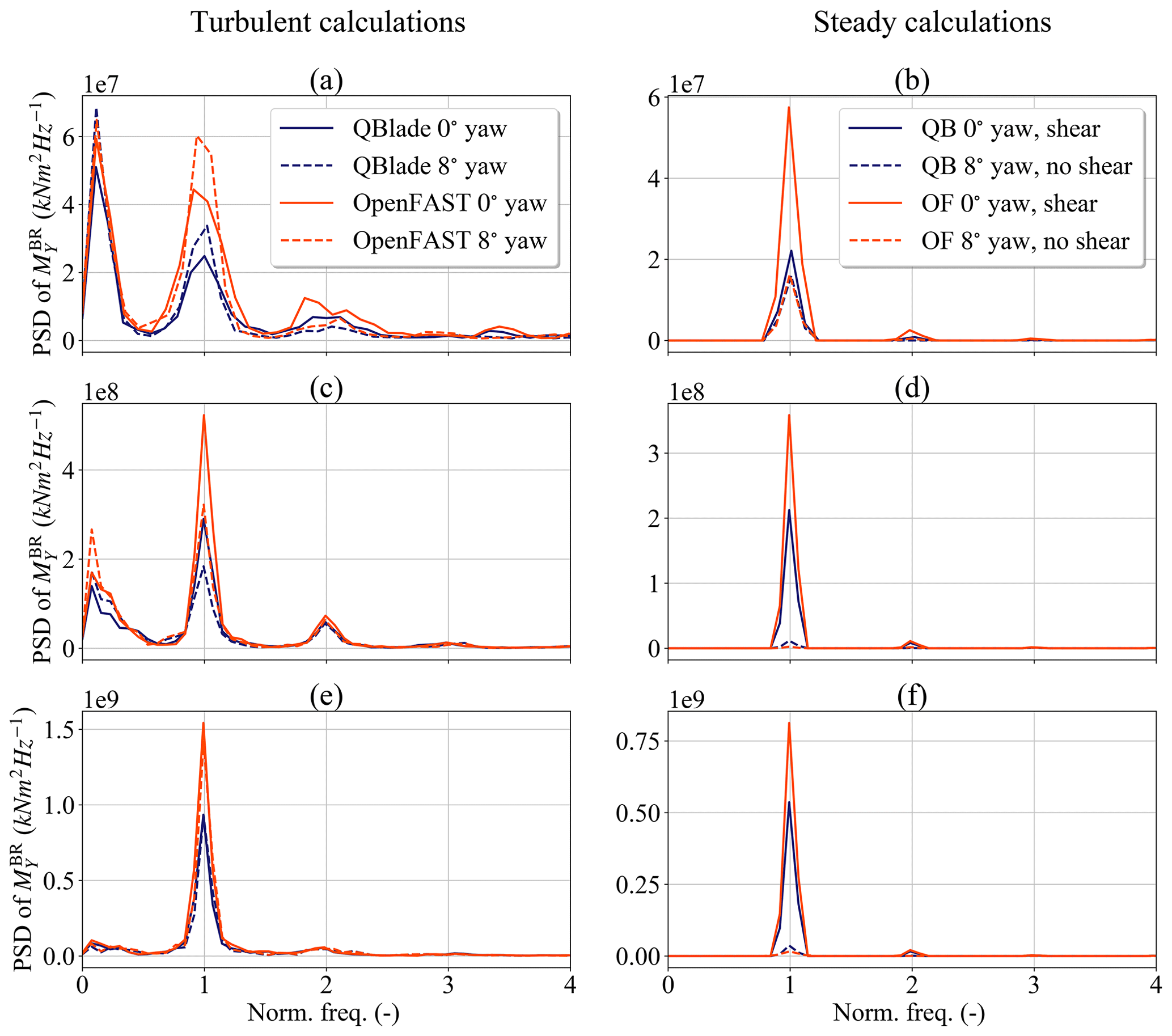
Figure 9Power spectral density plots for at different wind speeds: (a) turbulent calculations at 8 m s−1 wind speed, (b) steady calculations at 8 m s−1 wind speed, (c) turbulent calculations at 14 m s−1 wind speed, (d) steady calculations at 14 m s−1 wind speed, (e) turbulent calculations at 20 m s−1 wind speed and (f) steady calculations at 20 m s−1 wind speed.
5.3 Discussion
To better understand the differences in the fatigue loads and the variability of the controller signals, we can categorize the wind speed bins into three qualitatively different wind speed regions: Regions A–C.
-
Region A includes wind speed bins between 4 and 10 m s−1. In this region, the turbine is below the rated wind speed and hence the controller seeks to maximize energy capture. The pitch controller is largely inactive and the tip speed ratio of the turbine is above or close to the turbine's optimal tip speed ratio. For the aerodynamic loads this means that the axial induction factor is relatively large. Therefore, the differences in the aerodynamic modeling will be large and their influence on the turbine loads significant.
-
Region B encompasses wind speed bins between 10 and 16 m s−1. In this region, the transition between below-rated power and above-rated power operations of the controller occurs. Small differences in aerodynamic loads can trigger this transition and significantly affect the turbine loading. This is because the thrust on the rotor is highest around the rated wind (Fig. 4a) and the activation of the pitch controller influences the thrust considerably. In this region, the tip speed ratio of the turbine is still close to the optimum. Hence the axial induction is still large making differences in aerodynamic models relevant for turbine loading.
-
Region C covers wind speed bins between 18 and 24 m s−1. Here, the blade pitch angle is relatively high and the rotor speed is close to the rated rotor speed ΩR. With higher wind speeds the wake is convected faster downstream, effectively reducing the effect of its induced velocity on the rotor plane. This translates into smaller values of axial induction factors on the blade elements and on the rotor as a whole. Hence, the global effect of the different aerodynamic models on the controller behavior decreases. This in turn reduces the loading differences for certain turbine loads.
Because we are analyzing turbulent load calculations with varying wind speed, the limits between the regions cannot be exactly defined. We will consider one wind speed bin for each region as a representative set of simulations for that region. For each chosen wind speed bin, the qualitative turbine behavior will be the same as in the corresponding region described above. For Region A the chosen wind speed bin is 8 m s−1, for Region B the wind speed bin is 14 m s−1 and for Region C the wind speed bin is 20 m s−1. We will concentrate on the same turbine loads as in Fig. 8 to limit the extension of this section.
It should be stressed here that the analysis done in this section is valid only for the two particular aerodynamic codes considered in this study. The LLFVW implementation of QBlade does not take into account the interaction between the vorticity of the wind shear and the vorticity due to the wake. This affects the shape of the turbine wake and influences the loading on the turbine (Branlard et al., 2015). The choices of the engineering correction models used in AeroDyn are also particular for this code. Other BEM codes implement engineering models and the coupling between them differently (Madsen et al., 2020).
5.3.1 Blade root out-of-plane bending moment
Figure 9 shows the power spectral density (PSD) plots of for several BEM and LLFVW simulations. Each row of the subplots in the figure corresponds to one of the aforementioned regions. The left column shows PSD plots of the results from turbulent wind load calculation. The right column shows the PSDs of 200 s simulations with steady inflow conditions. The latter column will help us understand the source of the differences in the fatigue loads between both codes. As with the turbulent calculations, an additional 100 s was simulated and discarded in the analysis to allow the wake in the steady LLFVW simulations to build up.
Figure 9a and b show the PSD plots of for simulations in the 8 m s−1 wind speed bin – i.e., Region A. In Fig. 9a the solid lines represent turbulent wind simulations with a 0∘ yaw error, while the dashed lines represent simulations with 8∘ yaw error. For Fig. 9b, the solid lines represent results from steady wind simulations without yaw error but with a 0.2 wind shear exponent, while the dashed lines represent results from simulations with 8∘ yaw error and a wind shear exponent of 0. The idea of the simulations in Fig. 9b is to isolate different aerodynamic phenomena to see their individual contribution to the fatigue loading. Apart from the tip- and root-loss model, the major difference of the aerodynamic models in the solid line simulations is the treatment of the nonhomogeneous wind speed distribution on the rotor disc. In contrast, the major difference of the aerodynamic models in the dashed line simulations is the treatment of the oblique inflow.
When we consider the PSDs of the turbulent load calculations (Fig. 9a), we can see that the are two main peaks at different frequencies in the PSD. One peak is at a low, below once-per-revolution (1P) frequency. This is the frequency region where the controller is active.
The second peak is at the 1P frequency. If we compare the amplitudes between the aerodynamic codes at that frequency we can see that, for both the 8 and 0∘ yaw error simulations, the amplitude of the 1P peak in the PSD of the BEM simulations is visibly larger than the corresponding peak in the LLFVW simulations. The main source of this difference between both codes is the effect that the nonhomogeneous wind field – arising for example from the wind shear – has on the local blade aerodynamics. As Fig. 9b shows, simulating the turbine in sheared inflow leads to the largest differences between both codes in the load prediction at the 1P frequency of PSD(). The reason for this difference has already been identified and explained by other authors – e.g., Madsen et al. (2012), Boorsma et al. (2016), Madsen et al. (2020) – and will only be briefly mentioned here. According to Moriarty and Hansen (2005), AeroDyn calculates the local thrust coefficient using the average inflow wind speed from the rotor; a procedure also done in other BEM codes (Madsen et al., 2012). This choice has an averaging effect on the local axial-induced velocity when the turbine is simulated with sheared inflow. As a result, the local angle of attack sees a higher amplitude in the 1P variations compared to when the scenario simulated with a LLFVW code. In the latter, the local three-dimensional induction field is implicitly modeled through the induced velocities from the bound and wake vortices. The result is a better tracking of the local axial-induced velocity with the LLFVW simulations. Having higher angle of attack variations in BEM simulations leads to higher 1P variations in the local lift forces and ultimately to higher 1P variations in (compared to ).
These loading differences are also seen between different implementations of BEM codes. Madsen et al. (2020) implement a BEM model on a polar grid. This code also allows for a better tracking of the local induction variations on the blades compared to an annular averaged BEM approach. This polar implementation of a BEM-type code leads to a significant reduction in fatigue loads when compared to the more common annular-averaged BEM approach. They also show that, for large wind turbines, the rotational sampling of the turbulent inflow is an important contributor to load differences between the different BEM implementations. This rotational sampling also contributes to the loading differences at the 1P frequency in Fig. 9a.
The behavior of the PSD plots changes when we compare simulations in Region B (Fig. 9c). There are still two major peaks in the PSD: again one is at the low frequency of the controller and the other at the 1P frequency. In contrast to Region A, the 1P peak is now much more pronounced than the low-frequency peak. Also, there are differences between the aerodynamic codes at both frequency peaks in Region B. The reasons for the differences at the 1P frequency are the same as in Region A (Fig. 9d). We can understand the differences at the low-frequency region of the controller if we recall Fig. 5d. In Region B the turbine controller is often transitioning between below-rated power and above-rated power operations, thereby reaching maximum thrust. Because of the slightly higher aerodynamic torque from the LLFVW simulations, the turbine controller is able to keep ΩR and rated power for a higher percentage of time compared to the BEM simulations. The smaller variations in ΩLLFVW (Figs. 5d and 6a) also lead to smaller variations in rotor thrust and hence smaller variations in . The higher aerodynamic torque and smaller variation in ΩLLFVW also lead to smaller variations in θLLFVW (Figs. 5c and 6b). Again, this lowers the variation in rotor thrust and ultimately the variation in .
We finally consider Region C in Fig. 9e and f. Here, the 1P frequency peak dominates the PSD and is still the frequency where the differences between the codes lie. The reason for the differences is again the different treatment of the nonhomogeneous wind field in both codes. The variation in the controller signals in this region is comparable between both codes (Fig. 6). The same holds true for the effect of the controller action on . Yet this load contribution to the PSD() is overshadowed by the load contribution from the 1P frequency.
5.3.2 Tower base fore–aft bending moment
Like , the tower base fore–aft bending moment also shows large differences in the lifetime DELs. Figure 10 shows the PSD plots for the sensors in Regions A–C. The rows and columns are organized in the same way as in Fig. 9.
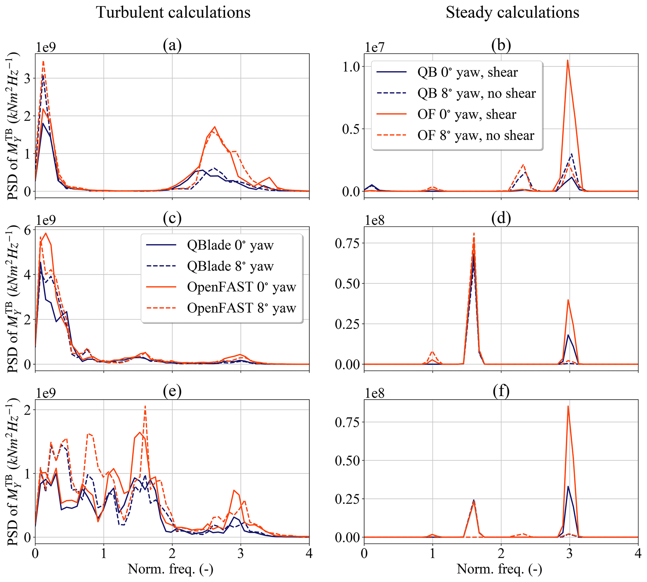
Figure 10Power spectral density plots for at different wind speeds: (a) turbulent calculations at 8 m s−1 wind speed, (b) steady calculations at 8 m s−1 wind speed, (c) turbulent calculations at 14 m s−1 wind speed, (d) steady calculations at 14 m s−1 wind speed;, (e) turbulent calculations at 20 m s−1 wind speed and (f) steady calculations at 20 m s−1 wind speed.
For turbulent wind speed calculations in Region A (Fig. 10a), we can see that the main differences in PSD() from both aerodynamic codes lie close to the 3P frequency. The source of this difference comes mostly from the treatment of the nonhomogeneous wind field, as can be seen in Fig. 10b. The reason for this is as follows. Since the amplitude of the 1P frequency component of in sheared flow is lower than for (Fig. 9b), the amplitude of the PSD at the tower-passing frequency – i.e., 3P – will also be lower for the LLFVW simulations. The fact that the differences in Fig. 10a do not lie exactly on the 3P frequency comes from the varying rotor speed in the simulations. The normalization of the frequencies was done using the average rotor speed of each simulation.
If we now concentrate on Region B simulations, we can see in Fig. 10c that the dominant frequencies in PSD() for all simulations are the low sub-1P frequencies. It is also this frequency range of the PSD that contains the largest differences between both codes. While there are some differences in the PSD at the 3P frequencies due to wind shear (Fig. 10d), the contribution of this frequency is significantly smaller than the contribution of the low-frequency range. As in the case of , the reason for this loading difference can be traced back to the higher aerodynamic torque from the LLFVW simulations. It leads to lower variations in σ(ΩLLFVW) and σ(θLLFVW) in this region (Fig. 6) and ultimately lower variations in rotor thrust.
For simulations in Region C the PSD() of both codes is comparable and at the same time more complicated (Fig. 10e). There are several frequency regions in which the PSD of the BEM simulations is higher than the PSD of the LLFVW simulations. For the 3P frequency, the difference is due to the treatment of the nonhomogeneous wind field (Fig. 10f) but its contribution to the PSD is small compared to the lower frequencies.
We note a large difference in peaks of PSD() at about 1.5P frequency in Fig. 10e. This peak is also present in Fig. 10d and f. The frequency corresponds to an absolute frequency of 0.25 Hz, which is the natural frequency of the first tower fore–aft and side–side mode of the turbine (Bak et al., 2013). In the simulations we saw that the damping of the mode was low in the side–side direction and contributed to the oscillations of . As for the tower fore–aft mode, its contribution to PSD() is also significant in Region C and the peak for the BEM simulations is consistently higher. This indicates that the aerodynamic damping of the first tower fore–aft mode is higher for the LLFVW simulations than for the BEM simulations.
5.3.3 Yaw-bearing roll moment
In absolute terms, is the load sensor with the smallest variation in amplitude. Therefore, small differences in loading will have a large influence on the relative contribution to the fatigue loads of this sensor. This load component is affected by the generator torque and by the side–side force acting on the rotor hub. The latter force causes a roll moment due to the vertical offset of the rotor hub to the yaw bearing. A similar analysis was performed for this sensor as was done for and , although for brevity only the results will be stated here.
For turbulent simulations in Region A, the main difference in PSD() lies in the low-frequency range where the controller is active. It is therefore the variability of the generator torque that is the source of the load differences in this region. It could be argued that the variability of Ω for this particular wind speed bin is larger in the LLFVW simulations (see Fig. 6a). Yet the higher variability of the electrical power in Region A for the BEM simulations seen in Fig. 5b indicates that in this region there is a higher fluctuation in the generator torque which causes the higher fatigue loads of . It is also this phenomenon that is the source of the differences in Region B.
When we consider Region C, we can see in Fig. 8b that the normalized is close to 1, indicating that the fatigue loads derived from the LLFVW simulations are almost the same as the ones derived from the BEM simulations. Yet the PSD() reveals that at different frequencies there are different loading peaks for BEM and LLFVW simulations. As in Regions A and B, there is a slightly higher peak at the low frequencies of the controller in the BEM simulations. At the 0.25 Hz frequency though, there is a higher peak for the LLFVW simulations. The reason for this is the lowly damped oscillations of the first tower side–side mode mentioned above. This side–side oscillation of the tower top is not directly influenced by the aerodynamics. While the relative contribution of the first tower fore–aft mode to PSD() is moderate (Fig. 10f), the relative contribution of the first tower side–side mode to PSD() is much higher. Because of the small absolute variations in this load signal, the side–side forces present in the hub contribute significantly to the fatigue loads. In our study, BEM simulations show higher oscillations for certain wind speeds and turbulent seeds, while in other cases the LLFVW show higher oscillations. For higher wind speeds in particular, the side–side oscillations of the tower top tend to have a higher amplitude in the LLFVW simulations, explaining the higher 1 Hz DELs of for the latter aerodynamic code seen in this region.
5.3.4 Yaw-bearing tilt moment
The last sensor analyzed in this section is . As with the yaw-bearing roll moment, we will only include the results of the discussion in this section.
For Region A, there are two peaks where PSD is higher than PSD. One is at the 3P frequency and the other at the below 1P frequencies. The latter region corresponding to the frequencies of the time-varying turbulent wind and the resulting controller reaction. These peaks can be explained by the fact that one source of – measured in a nonrotating frame of reference – is the nonuniform distribution of from the three blades, which is measured in a rotating frame of reference (Burton et al., 2011, 501–503). In particular, amplitude changes at the 1P frequency of PSD() contribute to amplitude changes at the 0P frequency (or very low frequencies in cases of varying wind speed) of PSD(). Changes at the 1P frequency of PSD() also contribute to amplitude changes at the 2P frequency of PSD(), although the contribution of the loads at this frequency to the fatigue loads of is negligible for three-bladed turbines. Changes at the 2P frequency in the PSD() contribute to changes at the 1P and 3P frequencies in PSD(). Again, only the 3P frequency in PSD() has an important load contribution for this sensor in the case of a three-bladed turbine. As we can see in Fig. 9a and b, the 1P and 2P peaks in the PSD of have a higher amplitude than the peaks from . The reason for these differences comes from the effect of the nonhomogeneous wind field on the local blade aerodynamics. This is also an important contributor to the differences in the case of .
This phenomenon is also responsible for the fatigue load differences in Regions B and C. As we can see in Fig. 9c and e, the load peak at the 1P frequency becomes more dominant in PSD(), increasing the contribution of the low-frequency peak of PSD() to the fatigue loads. While the normalized values of remain fairly constant for higher wind speed bins (Fig. 8a), the normalized values of increase and get closer to 1. The cause of this apparent discrepancy can be explained if we consider a second source of yaw-bearing tilt moment: the axial force on the rotor hub from the rotor thrust. Because of the vertical offset between the hub and the yaw bearing, variations in rotor thrust will lead to variations in . Recalling Fig. 6b, we can see that for wind speed bins of 16 m s−1 and above, increases towards a normalized value of 1. This leads to the result that the differences in rotor thrust variations between BEM and LLFVW simulations decrease, in turn reducing the differences in amplitude of variations.
In the previous section, we discussed the contribution of the periodic oscillations on the turbine loading. This section considers the extreme events that the turbine sensors experienced in the turbulent wind load calculations. The ultimate state analysis was done for all the sensors listed in Table 3. We analyze the deflection and control signals in the first subsection and the load sensors in the second subsection. The last subsection discusses the differences of the extrema and the reasons behind these differences.
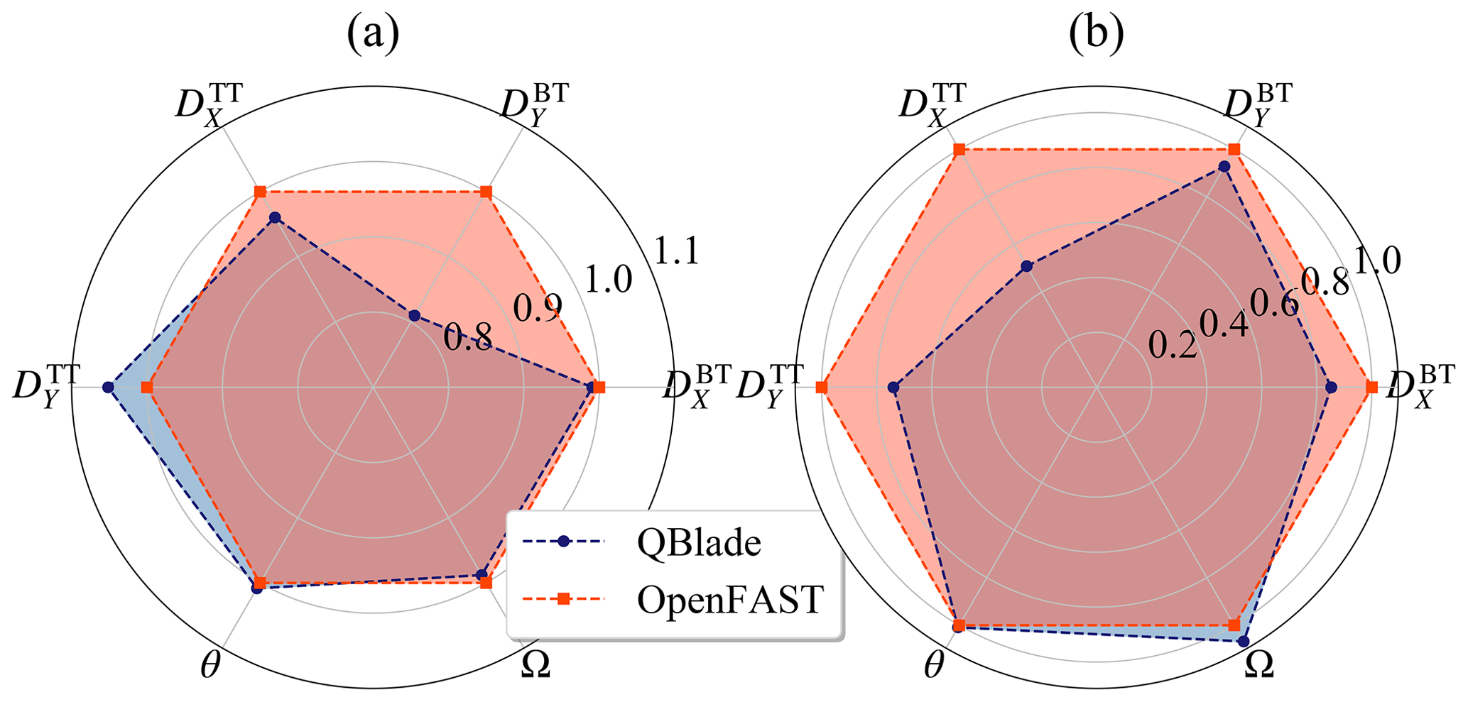
Figure 11Normalized extreme values of deflections and controller signals: (a) maxima and (b) minima.
The extreme values presented in this subsection are obtained by taking the maximum and minimum occurring values in the time series of all the simulations. In addition, the extreme values of the blade-related sensors – i.e., , , , and θ – are obtained from one blade only. The same blade was considered in the analysis of the BEM and the LLFVW simulations. For this study, it is considered that the extreme event analysis of one blade is representative of all three blades.
Analogously to the fatigue analysis, we will use the notation MaxMin(⋅)BEM for the maximum and minimum of a sensor in the BEM simulations. The extrema for the LLFVW simulations will have the corresponding subscript. Although we present the results for all sensors, we will concentrate our discussion and analysis on the out-of-plane-related sensors. These sensors are the most directly affected by the differences in the aerodynamic models.
6.1 Deflections and controller signals
Figure 11 shows the normalized extreme values of the blade tip and tower top deflections as well as the pitch angle and rotor speed. It is clear from this figure that using different aerodynamic models in load calculations also affects the extrema of the considered sensors.
When looking at the blade deflections, it is remarkable to see that the extrema of are very similar in both calculations. From the higher 1 Hz DELs of in the BEM simulations at wind speeds close to the rated wind speed, we would expect to see blade deflections with higher amplitudes in the BEM simulations and hence larger extrema of . While on average the amplitude of in the BEM simulations is larger than in the LLFVW calculations, the normalized value of Max is 0.99.
The tower top deflections show larger differences in extreme values from the different calculations than the blade tip deflections. If we consider the extrema of the fore–aft deflection, we see that the normalized values of Max and Min are 0.96 and 0.51, respectively.
Finally, Fig. 11 also shows the normalized extreme values of the pitch angle and rotor speed. The extrema of the pitch angle θ are very similar in both codes. The rotor speed Ω also shows small differences in the extrema. The Max(Ω)LLFVW is 0.99.
6.2 Loads
Performing load calculations with different aerodynamic models also has an impact on practically all the considered extreme loads of the turbine, as Fig. 12 shows.
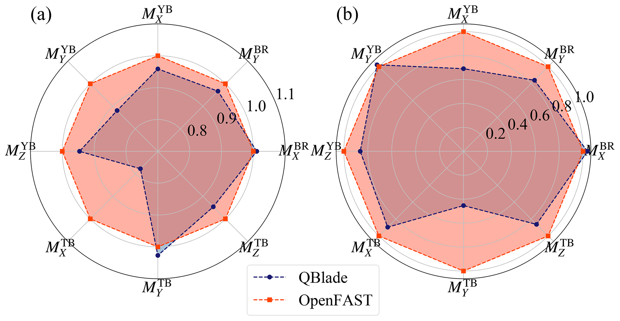
Let us start with the blade root loads. We can see in Fig. 12 that the normalized extrema of are very similar in both calculations. This correlates with the fact that the extreme values of in Fig. 11 were also very similar between both codes. The normalized Max and Min are 0.97 and 0.84, respectively.
In the case of the yaw bearing, the most notable difference in extreme loads occurs for the tilting moment. The normalized Max is 0.88.
For the tower base loads we see large differences in the extrema of the fore–aft bending moment. The normalized values of Max and Min are 1.02 and 0.45. A deeper analysis of these differences in the extreme loads is presented in the next section.
6.3 Discussion
As with the fatigue loads, the reason for these differences in the extreme loads must ultimately come from the different aerodynamic models.
In order to limit the extension of this analysis, we will only consider a selection of the sensors. These are , , , and as they show large deviations and are directly influenced by the aerodynamic loads. While doing the ultimate load analysis, we noted that the extrema of BEM and LLFVW simulations did not necessarily occur in the same simulation or even the same wind speed bin. In the following analysis we will always present the load case where the highest (absolute) extreme value of the sensors occurred, whether it happened for the BEM calculations or the LLFVW calculations. Thus if the maximum of was higher for the BEM code, for example, we will include the time series analysis of the BEM load case and show the corresponding LLFVW load case as a comparison. The load case where the maximum of in the LLFVW simulations occurred will not be analyzed.
6.3.1 Tower loads and deflections
For the extreme values of the tower sensors, we see in Figs. 11 and 12 that Max but Max. These extreme values result from different events happening at different time instants. Curiously, these events share the same load case that comes from the 12 m s−1 wind speed bin.
A selection of the load case time series is shown in Fig. 13. The time instant where Max occurs is around 450 s of simulation time. The time instant where Max occurs is around 650 s of simulation time.
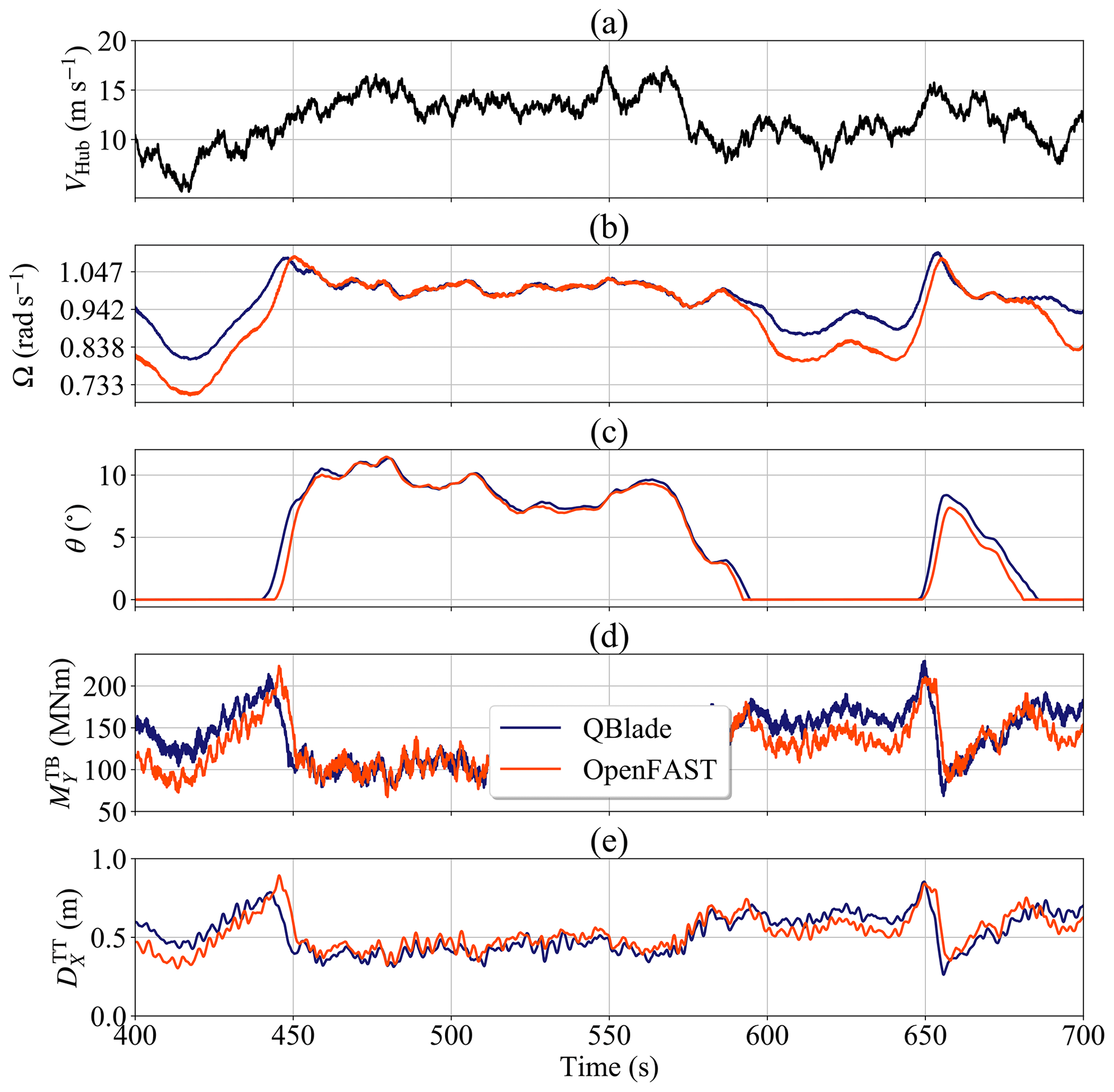
Figure 13Time series of the extreme tower event: (a) wind speed at hub height, (b) rotor speed, (c) pitch angle, (d) tower base fore–aft bending moment and (e) tower top fore–aft deflection.
Let us focus on Max first. As we can see in Fig. 13a, there is an increase in the hub wind speed from just above 5 m s−1 to about 12 m s−1 in the simulation time interval between 400 and 450 s. For that time interval, ΩBEM takes values that are roughly 0.1047 rad s−1 lower than ΩLLFVW (Fig. 13b). When the hub wind speed increases to about 12 m s−1 both ΩBEM and ΩLLFVW reach ΩR, which activates the pitch controller. The rotational acceleration of the rotor is smaller in the LLFVW simulations, allowing more time for the controller to increase θLLFVW (Fig. 13c) and limit the effect of the aerodynamic thrust on (Fig. 13d) and (Fig. 13e). For the BEM simulation, on the other hand, we see that the rotational acceleration is higher. This gives the controller less time to increase θBEM and hence the wind speed increase generates a higher rotor thrust. This leads to higher values of and the recorded maximum of .
If we now consider on Max, we can see that there is a similar turbine configuration between 600 and 650 s that leads to the differences in maxima between BEM and LLFVW simulations. This time, a sudden wind gust at around 650 s increases the hub wind velocity from about 10 to 15 m s−1. There is again a difference of around 0.1047 rad s−1 between ΩBEM and ΩLLFVW. Yet in this event, the rotational accelerations from both simulations have very similar values. Because ΩLLFVW is almost 0.942 rad s−1 just before the gust, the wind velocity jump leaves ΩLLFVW at a higher value compared to ΩBEM at the time instant the pitch controller is activated to feather out the overshoot. The higher value of ΩLLFVW increases the tip speed ratio and hence the axial induction of the rotor, when compared to the axial induction in the BEM simulation. An increase in the instantaneous induction results in a higher thrust on the rotor. This leads to the recorded maximum of .
The difference in the controller behavior affecting the maxima of the tower sensors can be traced back to the higher aerodynamic torque of the LLFVW simulations (Fig. 3b) that lead to higher values of ΩLLFVW in the below-rated power wind regime (Figs. 4d and 5d). Especially for wind speeds around the rated wind speed, small differences in rotor speed cause the transition between below-rated power and above-rated power operations of the controller, influencing significantly the loading on the turbine.
6.3.2 Out-of-plane root-bending moment and tip deflection of the blade
A similar analysis to that in the previous subsection was also carried out for and . For brevity, only the findings will be presented here.
For the BEM simulations, Max and Max occurred for a load case simulation at the wind speed bin of 12 m s−1. Similar to Fig. 13, the differences in the blade root loading and tip deflection come from a lower θBEM at the moment the wind turbine encountered a small wind gust. As with the tower sensors, there is again a difference of around 0.1047 rad s−1 between ΩBEM and ΩLLFVW just before the gust, leading to the lower values of θBEM. This difference can be traced back to the higher aerodynamic torque from the LLFVW simulations, thus affecting the transition of the controller operation modes.
6.3.3 Yaw-bearing tilt moment
From Fig. 12 we see that the normalized value of Max is 0.88. We will again only present the results of the analysis to limit the extent of this section.
The maxima of occurred in a load case simulation with 24 m s−1 average wind speed for both the BEM and LLFVW simulations. In this load case, the controller behavior is almost identical. The most relevant difference is that (because of the higher aerodynamic torque in the LLFVW simulations) the average value of θLLFVW is slightly higher than the value of θBEM, a behavior also seen in Fig. 5c. As a consequence the average rotor thrust in the BEM simulation is also slightly higher and, due to the vertical offset between rotor hub and yaw bearing, so is the average value of . It should be noted that for this simulation ΩBEM and ΩLLFVW are practically identical, leading to coinciding rotor azimuth angles in both codes. The extreme event occurs at an azimuth angle of 65∘, meaning that the turbine is close to the Y configuration in which one blade is in front of the tower. This is the configuration of maximum . Because of different treatment of the nonhomogeneous wind field between the codes, the also has a higher energy content in the 3P frequency (see Sect. 5.3.4). The higher average value due to the thrust and the higher 3P oscillation of led to a higher maximum peak of , which also becomes the extreme value of this sensor of all simulations.
In this paper we analyzed the effect of two different aerodynamic models on the performance and especially on the loads of the DTU 10 MW RWT. The first aerodynamic model – used in the aeroelastic simulation software OpenFAST – is an implementation of the BEM method, the standard method used in the industry. The second aerodynamic model – used in TU Berlin's aeroelastic software QBlade – is an implementation of the LLFVW method.
We did a baseline comparison of both codes by calculating the performance of the turbine under constant uniform wind speeds, a configuration where many of the engineering correction models do not contribute to the aerodynamic loads. The performance coefficients of the turbine simulated with both codes were similar for all relevant wind speeds where the turbine is in power production. The largest differences were seen at wind speeds below the rated wind speed, where the axial induction factor plays an important role. Including measures to speed up the LLFVW simulations as well as elasticity did not have a significant impact on the performance of the wind turbine.
We also simulated the wind turbine under turbulent wind conditions following the requirements of the IEC 61400-1 Ed.3 DLC groups 1.1 and 1.2. The average performance of the turbine in the turbulent wind simulations is comparable to the performance in the idealized simulations with constant uniform wind speed. Yet there is considerable variation in the thrust and power of the turbine due to the unsteady aerodynamic phenomena present in the turbulent wind load calculations. Those variations are more marked in the BEM simulations than in the LLFVW simulations, with the former showing a higher activity in the controller signals – i.e., the rotor speed and the pitch angle. This leads to considerable differences in the fatigue and extreme loads of the turbine.
In order to quantify the differences in the fatigue loads, we carried out a fatigue analysis that includes the lifetime DELs and the per-wind-bin-averaged 1 Hz DELs of selected load sensors of the turbine. For the lifetime DELs, the LLFVW simulations show a 9 % decrease in DEL and DEL compared to the BEM simulations. Analyzing the averaged 1 Hz DELs, we found that the wind speed bins below the rated wind speed contribute the most to the decrease in the sensors' fatigue loads in the LLFVW simulations. For bins with higher wind speeds, the differences in fatigue loads of remain roughly constant and the differences in fatigue loads diminish. Further analysis showed that the main contributors to the differences in the fatigue loads of the sensors are the different way the nonhomogeneous wind field affects the local blade aerodynamics in each code and the higher average aerodynamic torque seen in the LLFVW calculations. The latter influenced the values of ΩLLFVW and – for wind speeds around the rated wind speeds – affected the transition of the controller between below-rated power and above-rated power operations. This had a significant effect on the turbine loading.
For the yaw-bearing moment, we found that the LLFVW simulations predicted a decrease of 4 % and 3 % in DEL and DEL, respectively. Analyzing the contributions of individual wind speed bins on the 1 Hz DELs of revealed that the load differences for this sensor arose from the same aerodynamic differences that contributed to the differences of and .
We also did an ultimate state analysis on the results of the turbulent wind load calculations. For the out-of-plane loads and deflections of the blade, we found that the BEM simulations predicted higher extrema than the LLFVW simulations. The maxima of and are 1 % and 3 % higher than their respective maxima in the LLFVW simulations. As for the tower sensors, we found that Max is 4 % higher and Max 2 % lower than their respective maxima in the LLFVW simulations. The reason for these differences could be traced back to the higher average aerodynamic torque in the LLFVW simulations, which caused differences in the transition of the turbine controller between operating modes and hence the loading. The higher aerodynamic torque in the LLFVW simulations and the different treatment of the nonhomogeneous wind field were the reasons for the differences in Max between both codes. In the case of this sensor, the results from LLFVW simulations predicted a decrease in Max by 12 %.
The results of this paper show that there are significant differences in the fatigue and extreme loads if we use a higher-order aerodynamic model in the load calculations. The fact that lower fatigue loads were obtained for the considered sensors when using the LLFVW method indicates that there is a real potential to reduce the design loads of modern multi-megawatt wind turbines by adopting higher-order aerodynamic models in load calculations. Yet more work needs to be done before this can be stated as a general conclusion. In order to improve our quantification of the load differences, future work will include simulations with a higher-order representation of the structural dynamics. By including the torsional degree of freedom, we will be able to model the flap–twist coupling that greatly influences the loads on the turbine. In order to better quantify the differences in extreme loads, more DLC groups from the current guidelines and standards should be included. Performing an ultimate state analysis of the IEC 64100-1 DLC 1.1 and 1.2 groups gave us some insight into the influence of the aerodynamic codes on the extreme loads. Including DLC groups that are known to induce design driving extreme loads on the turbine will help us to better understand and quantify the effect of higher-order aerodynamic models on the extreme loads.
This appendix contains the wake-coarsening parameters we used in our LLFVW simulations. They are summarized in Table A1.
Table A1Wake-coarsening parameters for aerodynamic and aeroelastic LLFVW simulations.
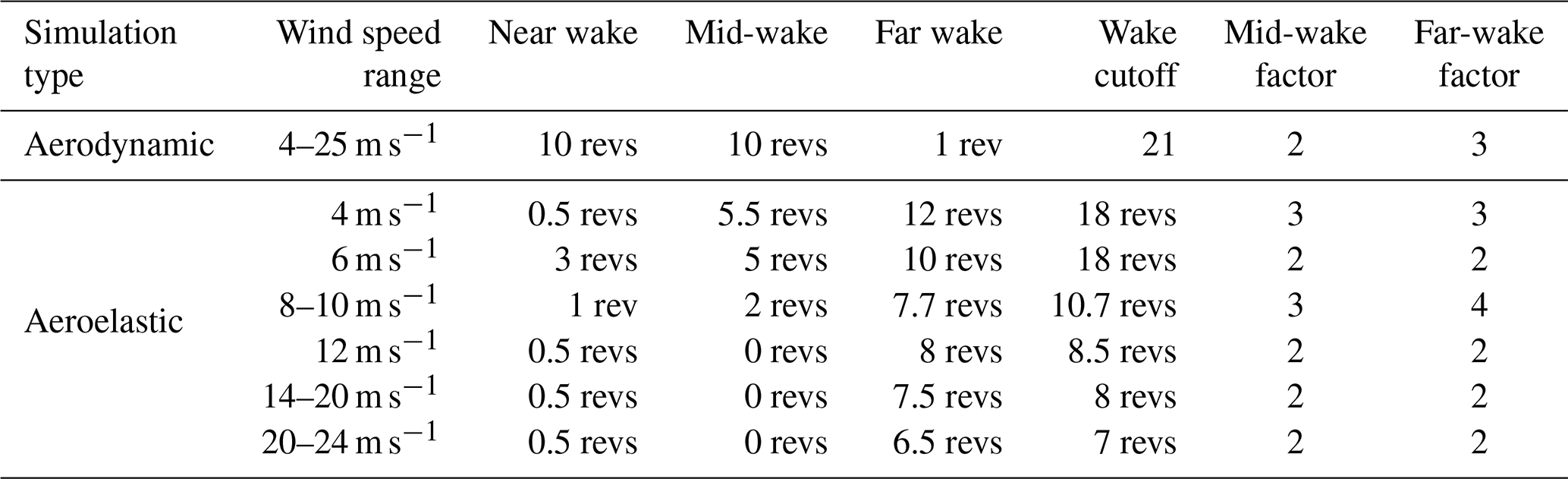
Both OpenFAST and QBlade are open-source code that is available online. The latest version of OpenFAST is available at https://github.com/OpenFAST (last access: 29 May 2019) (OpenFAST, 2019). The latest version of QBlade is available at https://sourceforge.net/projects/qblade/ (last access: 5 June 2020) (QBlade, 2020). The version of QBlade used in this paper, which includes the structural model, will be made available soon. The time series for the BEM and LLFVW calculations used in this paper are stored in the OpenFAST binary format. They can be made available upon request. The figures described but not shown in Sects. 5 and 6 can be made available upon request.
SPB prepared the manuscript with the help of all co-authors. DM is the main developer of QBlade and developed the aerodynamic code. JS developed the structural code. SPB and FP performed the calculations and the analysis of the results. AB and COP provided assistance with the paper review.
The authors declare that they have no conflict of interest.
This article is part of the special issue “Wind Energy Science Conference 2019”. It is a result of the Wind Energy Science Conference 2019, Cork, Ireland, 17–20 June 2019.
Sebastian Perez-Becker wishes to thank WINDnovation Engineering Solutions GmbH for supporting his research.
This open-access publication was funded by Technische Universität Berlin.
This paper was edited by Katherine Dykes and reviewed by Emmanuel Branlard and Georg Raimund Pirrung.
Bak, C., Madsen, H. A., and Johansen, J.: Influence from Blade-Tower Interaction on Fatigue Loads and Dynamics, in: Proceedings of the 2001 European Wind Energy Conference and Exhibition, Copenhagen, Denmark, 394–397, 2001. a
Bak, C., Johansen, J., and Andersen, P. B.: Three-Dimensional Corrections of Airfoil Characteristics based on Pressure Distributions, in: Proceedings of the European Wind Energy Conference and Exhibition, Athens, Greece, 1–10, 2006. a, b
Bak, C., Zahle, F., Bitsche, R., Kim, T., Yde, A., Henriksen, L. C., Andersen, P. B., Natarajan, A., and Hansen, M. H.: Design and Performance of a 10 MW Wind Turbine, Tech. Rep. I-0092, DTU Wind Energy, Roskilde, Denmark, 2013. a, b, c, d, e
Bergami, L. and Gaunaa, M.: ATEFlap Aerodynamic Model, a Dynamic Stall Model Including the Effects of Trailing Edge Flap Deflection, Tech. Rep. Risø-R-1792, DTU Wind Energy, Risø, Denmark, 2012. a
Boorsma, K., Hartvelt, M., and Orsi, L.: Application of the Lifting Line Vortex Wake Method to Dynamic Load Case Simulations, J. Phys.: Conf. Ser., 753, 022030, https://doi.org/10.1088/1742-6596/753/2/022030, 2016. a, b, c, d
Boorsma, K., Greco, L., and Bedon, G.: Rotor Wake Engineering Models for Aeroelastic Applications, J. Phys.: Conf. Ser., 1037, 062013, https://doi.org/10.1088/1742-6596/1037/6/062013, 2018. a
Borg, M., Mirzaei, M., and Bredmose, H.: LIFES50+ Deliverable D1.2: Wind Turbine Models for the Design, Tech. Rep. E-101, DTU Wind Energy, Risø, Denmark, 2015. a
Branlard, E., Papadakis, G., Gaunaa, M., Winckelmans, G., and Larsen, T. J.: Aeroelastic Large Eddy Simulations Using Vortex Methods: Unfrozen Turbulent and Sheared Inflow, J. Phys.: Conf. Ser., 625, 012019, https://doi.org/10.1088/1742-6596/625/1/012019, 2015. a
Buhl, M. L. J.: Crunch Software, available at: https://nwtc.nrel.gov/Crunch, last access: 27 January 2018. a
Burton, T., Jenkins, N., Sharpe, D., and Bossanyi, E. A.: Wind Energy Handbook, 2nd Edn., John Wiley & Sons Ltd., West Sussex, UK, 2011. a, b, c
Chen, J., Shen, X., Zhu, X., and Du, Z.: Influence of Wake Asymmetry on Wind Turbine Blade Aerodynamic and Aeroelastic Performance in Shear/Yawed Wind, J. Renew. Sustain. Energ., 10, 053309, https://doi.org/10.1063/1.5030671, 2018. a
Hansen, M. H., Henriksen, L. C., Hartvig, M., and Christian, L.: Basic DTU Wind Energy Controller, Tech. Rep. E-0028, DTU Wind Energy, Risø, Denmark, 2013. a
Hansen, M. O. L.: Aerodynamics of Wind Turbines, 2nd Edn., Earthscan, London, UK, 2008. a
Hauptmann, S., Bülk, M., Schön, L., Erbslöh, S., Boorsma, K., Grasso, F., Kühn, M., and Cheng, P. W.: Comparison of the Lifting-Line Free Vortex Wake Method and the Blade-Element-Momentum Theory regarding the simulated Loads of Multi-MW Wind Turbines, J. Phys.: Conf. Ser., 555, 012050, https://doi.org/10.1088/1742-6596/555/1/012050, 2014. a, b, c
Hayman, G. J.: MLife Theory Manual for Version 1.00, Tech. rep., NREL, Golden, Colorado, 2012. a, b
IEC 61400-1 Ed. 3: IEC 61400-1: Wind Turbines – Part 1: Design Requirements, Standard, International Electrotechnical Commission, Geneva, Switzerland, 2005. a, b, c
Iribas, M., Hansen, M. H., Mahmood, M., Tibaldi, C., Natarajan, A., Bossanyi, E., Stock, A., Jamieson, P., Leithead, W., and Schlipf, D.: INNWIND Deliverable 1.42: Methodology for Feed-Forward Control Strategies using Nacelle or Blade Based Sensors and Distributed Control, Tech. rep., INNWIND.eu, available at: http://www.innwind.eu/publications/deliverable-reports (last access: 5 June 2020), 2015. a
Jamieson, P.: Innovation in Wind Turbine Design, 2nd Edn., John Wiley & Sons Ltd., West Sussex, UK, 2018. a
Jeong, M., Kim, S., Lee, I., and Yoo, S.: Wake Impacts on Aerodynamic and Aeroelastic Behaviors of a Horizontal Axis Wind Turbine Blade for Sheared and Turbulent Flow Conditions, J. Fluids Struct., 50, 66–78, https://doi.org/10.1016/j.jfluidstructs.2014.06.016, 2014. a
Jonkman, J.: Modeling of the UAE Wind Turbine for Refinement of FAST_AD, Tech. Rep. TP-500-34755, NREL, Golden, Colorado, 2003. a
Jonkman, J., Butterfield, S., Musial, W., and Scott, G.: Definition of a 5-MW Reference Wind Turbine for Offshore System Development, Tech. Rep. TP-500-38060, NREL, Golden, Colorado, 2009. a
Jonkman, J. M.: Overview of the ElastoDyn Structural-Dynamics Module, in: NREL Wind Turbine Modeling Workshop, Bergen, Norway, available at: https://wind.nrel.gov/public/jjonkman/Presentations/WindTurbineModelingWorkshop_1409_NORCOWE_BergenNorway/3_ElastoDyn_Jonkman.pdf (last access: 5 June 2020), 2014. a
Jonkman, J. M. and Buhl, M. L. J.: FAST User's Guide, Tech. Rep. EL-500-38230, NREL, Golden, Colorado, https://doi.org/10.2172/15020796, 2005. a, b
Madsen, H. A., Riziotis, V., Zahle, F., Hansen, M. O. L., Snel, H., Larsen, T. J., Politis, E., and Rasmussen, F.: Blade Element Momentum Modeling of Inflow with Shear in Comparison with Advanced Model Results, Wind Energy, 15, 63–81, https://doi.org/10.1002/we.493, 2012. a, b, c, d, e, f
Madsen, H. A., Larsen, T. J., Pirrung, G. R., Li, A., and Zahle, F.: Implementation of the Blade Element Momentum Model on a Polar Grid and its Aeroelastic Load Impact, Wind Energ. Sci., 5, 1–27, https://doi.org/10.5194/wes-5-1-2020, 2020. a, b, c, d
Marten, D., Wendler, J., Nayeri, C. N., and Paschereit, C. O.: Development and Application of a Simulation Tool for Vertical and Horizontal Axis Wind Turbines, in: Proceedings of the ASME Turbo Expo, San Antonio, Texas, https://doi.org/10.1115/GT2013-94979, 2013a. a
Marten, D., Wendler, J., Pechlivanoglou, G., Nayeri, C. N., and Paschereit, C. O.: QBlade: An Open Source Tool for Design and Simulation of Horizontal and Vertical Axis Wind Turbines, Int. J. Emerg. Technol. Adv. Eng., 3, 264–269, 2013b. a
Marten, D., Lennie, M., Pechlivanoglou, G., Nayeri, C. N., and Paschereit, C. O.: Implementation, Optimization and Validation of a Nonlinear Lifting Line-Free Vortex Wake Module within the Wind Turbine Simulation Code QBlade, ASME J. Eng. Gas Turb. Power, 138, 072601, https://doi.org/10.1115/GT2015-43265, 2015. a, b, c
Moriarty, P. and Hansen, A.: AeroDyn Theory Manual, Tech. Rep. EL-500-36881, NREL, Golden, Colorado, https://doi.org/10.2172/15014831, 2005. a, b, c, d
OpenFAST: OpenFAST, available at: https://github.com/OpenFAST/openfast, last access: 28 May 2019. a, b
Perez-Becker, S., Saverin, J., Marten, D., Alber, J., Pechlivanoglou, G., and Paschereit, C. O.: Investigations on the Fatigue Load Reduction Potential of Advanced Control Strategies for Multi-MW Wind Turbines using a Free Vortex Wake Model, in: Proceedings of ASME Turbo Expo 2018, Oslo, Norway, V009T48A008, https://doi.org/10.1115/GT2018-76078, 2018. a, b, c
Pirrung, G., Riziotis, V., Madsen, H., Hansen, M., and Kim, T.: Comparison of a Coupled Near- and Far-Wake Model with a Free-Wake Vortex Code, Wind Energ. Sci., 2, 15–33, https://doi.org/10.5194/wes-2-15-2017, 2017. a, b
QBlade: QBlade, available at: https://sourceforge.net/projects/qblade, last access: 5 June 2020. a
Qiu, Y. X., Wang, X. D., Kang, S., Zhao, M., and Liang, J. Y.: Predictions of Unsteady HAWT Aerodynamics in Yawing and Pitching using the Free Vortex Method, Renew. Energ., 70, 93–106, https://doi.org/10.1016/j.renene.2014.03.071, 2014. a
Saverin, J., Marten, D., Pechlivanoglou, G., Nayeri, C. N., and Paschereit, C. O.: Coupling of an Unsteady Lifting Line Free Vortex Wake Code to the Aeroelastic HAWT Simulation Suite FAST, in: vol. 9, Proceedings of ASME Turbo Expo 2016: Turbine Technical Conference and Exposition GT2016, Seoul, South Korea, V009T46A002, https://doi.org/10.1115/GT2016-56290, 2016a. a
Saverin, J., Peukert, J., Marten, D., Pechlivanoglou, G., Paschereit, C. O., and Greenblatt, D.: Aeroelastic Simulation of Multi-MW Wind Turbines using a free Vortex Model coupled to a geometrically exact Beam Model, J. Phys.: Conf. Ser., 753, 082015, https://doi.org/10.1088/1742-6596/753/8/082015, 2016b. a, b, c
Simms, D., Schreck, S., Hand, M., and Fingersh, L. J.: NREL Unsteady Aerodynamics Experiment in the NASA-Ames Wind Tunnel: A Comparison of Predictions to Measurements, Tech. Rep. TP-500-29494, NREL, Golden, Colorado, https://doi.org/10.2172/783409, 2001. a
Snel, H. and Schepers, J.: Joint Investigation of Dynamic Inflow Effects and Implementation of an Engineering Method, Tech. Rep. ECN-C-94-107, ECN, Petten, the Netherlands, available at: https://publications.ecn.nl/E/1995/ECN-C--94-107 (last access: 5 June 2020), 1995. a
Snel, H., Schepers, G., and Siccama, N.: MEXICO Project: The Database and Results of Data Processing and Interpretation, in: Proceedings of the 47th AIAA Aerospace Sciences Meeting, Orlando, Florida, 2009-1217, https://doi.org/10.2514/6.2009-1217, 2009. a
Tasora, A., Serban, R., Mazhar, H., Pazouki, A., Melanz, D., Fleischmann, J., Taylor, M., Sugiyama, H., and Negrut, D.: Chrono: An Open Source Multi-Physics Dynamics Engine, in: Proceedings of the International Conference on High Performance Computing in Science and Engineering, Solan, Czech Republic, 19–49, https://doi.org/10.1007/978-3-319-40361-8_2, 2016. a
Van Garrel, A.: Development of a Wind Turbine Aerodynamics Simulation Module, Tech. Rep. ECN-C-03-079, ECN Wind Energy, Petten, the Netherlands, https://doi.org/10.13140/RG.2.1.2773.8000, 2003. a, b
Voutsinas, S.: Vortex Methods in Aeronautics: How to Make Things Work, Int. J. Comput. Fluid Dynam., 20, 3–18, https://doi.org/10.1080/10618560600566059, 2006. a
Voutsinas, S., Riziotis, V., and Manolis, D.: Advance Aeroelastic Modeling of Swept Rotor Blades, in: Proceedings of European Wind Energy Conference and Exhibition, Brussels, Belgium, 2011. a
Wang, Q., Jonkman, J. M., Sprague, M., and Jonkman, B.: BeamDyn User's Guide and Theory Manual, Tech. rep., NREL, Golden, Colorado, available at: https://nwtc.nrel.gov/BeamDyn (last access: 30 October 2017), 2016. a
Wendler, J., Marten, D., Pechlivanoglou, G., Nayeri, C. N., and Paschereit, C. O.: An Unsteady Aerodynamics Model for Lifting Line Free Vortex Wake Simulations of HAWT and VAWT in QBlade, in: Proceedings of ASME Turbo Expo: Turbine Technical Conference and Exposition GT2016, Seoul, South Korea, V009T46A011, https://doi.org/10.1115/GT2016-57184, 2016. a
- Abstract
- Introduction
- Methods
- Baseline comparison and performance under idealized conditions
- Design load calculations with turbulent wind
- Fatigue analysis of the design load calculation results
- Ultimate state analysis of the design load calculation results
- Conclusions
- Appendix A: Wake-coarsening parameters for the LLFVW simulations
- Code and data availability
- Author contributions
- Competing interests
- Special issue statement
- Acknowledgements
- Financial support
- Review statement
- References