Decreasing wind speed extrapolation error via domain-specific feature extraction and selection

Model uncertainty is a significant challenge in the wind energy industry and can lead to mischaracterization of millions of dollars' worth of wind resources. Machine learning methods, notably deep artificial neural networks (ANNs), are capable of modeling turbulent and chaotic systems and offer a promising tool to produce high-accuracy wind speed forecasts and extrapolations. This paper uses data collected by profiling Doppler lidars over three field campaigns to investigate the efficacy of using ANNs for wind speed vertical extrapolation in a variety of terrains, and it quantifies the role of domain knowledge in ANN extrapolation accuracy. A series of 11 meteorological parameters (features) are used as ANN inputs, and the resulting output accuracy is compared with that of both standard log-law and power-law extrapolations. It is found that extracted nondimensional inputs, namely turbulence intensity, current wind speed, and previous wind speed, are the features that most reliably improve the ANN's accuracy, providing up to a 65 % and 52 % increase in extrapolation accuracy over log-law and power-law predictions, respectively. The volume of input data is also deemed important for achieving robust results. One test case is analyzed in depth using dimensional and nondimensional features, showing that the feature nondimensionalization drastically improves network accuracy and robustness for sparsely sampled atmospheric cases.

1 Introduction

Challenges to the prediction of microscale atmospheric flows are well-documented, especially for complex terrain and forested regions (Baklanov et al., 2011; Krishnamurthy et al., 2013; Fernando et al., 2015, 2019; Sfyri et al., 2018; Yang et al., 2017; Berg et al., 2019; Wilczak et al., 2019; Pichugina et al., 2019). Poor or unfit parameterizations can lead to inaccurate flow prediction and extrapolation, producing large modeling uncertainties. Every location has unique flow features with variability that warrants a dedicated field campaign to develop and validate parameterization schemes befitting local forecasting. This process can still result in poor spatial representation of the site due to limitations in measurement technology, area covered by the field campaign, and site complexity.

Large extrapolation errors are particularly detrimental for wind farms, which rely on accurate wind speed extrapolation to estimate available wind resource and forecast output power. With the industry currently bracing for turbines up to 260 m tall, vertical extrapolation accuracy has become particularly important for the next generation of wind farms. The current industry standard of 1 % uncertainty per 10 m vertical extrapolation (Langreder and Jogararu, 2017) must be improved in order to increase the viability of such large-scale, powerful turbines. This would likely be particularly difficult to accomplish by using numerical models. In complex terrain, these models' parameterization schemes must be tuned for each individual region in order to obtain optimal results (Stiperski et al., 2019; Bianco et al., 2019; Olson et al., 2019; Akish et al., 2019), reducing the plug-and-play effectiveness of numerical modeling. Model results must also be scaled down to the desired finer resolutions, which can result in representativity error (Dupré et al., 2020). Machine learning models may ease such concerns as they can be rapidly, economically, and automatically parameterized; require no downscaling; and consistently improve with time and data availability. When properly applied, these machine learning techniques can likely aid in effectively calculating the rotor equivalent wind speeds for power curve measurements based on IEC 61400-12-1:2017 from either a met mast lower than hub height or a wind profiler with low data availability at higher heights (Türkan et al., 2016; Islam et al., 2017; Mohandes and Rehman, 2018). Additional applications in wind energy for such a technique range from feed-forward control of wind turbines or wind farms (Schlipf et al., 2013; Krishnamurthy, 2013; Kumar et al., 2015), prediction of yaw misalignment (Fleming et al., 2014), and optimizing wake-steering approaches (Fleming et al., 2019).

Neural networks have recently come into vogue due to the rapid increase in computational power alongside a plethora of available data. They are particularly skilled at pattern recognition and bias correction, having been used for various meteorological applications (McGovern et al., 2019; Hsieh and Tang, 1998). Multiple studies have shown that neural networks perform well when tasked with wind speed forecasting on a variety of timescales (Bilgili et al., 2007; More and Deo, 2003; Chen et al., 2019). However, wind speed measurements from meteorological towers or remote sensors must often be extrapolated in space as well as time to reach the location of interest (e.g., turbine hub height), adding another layer of forecasting complexity.

In a recent study, Mohandes and Rehman (2018) found that neural networks in conjunction with lidar data can accurately extrapolate wind speeds over flat terrain using wind speeds measured below the targeted height (extrapolation height). However, it is unclear whether this finding holds for more complex terrain. Knowledge of meteorological conditions and site characteristics could be essential for optimal extrapolation accuracy. In the same vein, Li et al. (2019) found that adding turbulence intensity as an input greatly improves wind speed forecasting accuracy, suggesting that the input feature set may be highly influential for machine learning tools applied to meteorological problems. Following such developments, the present study focuses on proper extraction and selection of meteorological features across multiple sites for a neural network designed for vertical extrapolation of wind speed. The novelty of this study is in addressing the following questions: first, is it possible to improve wind speed extrapolation accuracy under various terrain conditions using neural networks by invoking physics-based input features? Second, which atmospheric features should be selected to optimize the model's prediction capabilities?

Section 2 provides an introduction to neural networks and the list of input features utilized. Section 3 briefly describes the campaign sites and instrumentation utilized as well as measurement uncertainty. Section 4 presents findings of the investigation, and Sect. 5 provides analysis and discussion. Concluding remarks are given in Sect. 6.

2 Model overview

2.1 Neural network architecture

Artificial neural networks (ANNs) are a machine learning framework wherein a multilayered network of nodes attempts to compute an output from a given set of inputs while exploiting (often hidden) patterns underlying a given data structure. A classic feed-forward ANN layout is given in Fig. 1. These networks mimic the inner workings of the human brain and consist of four main elements: a layer of user-defined inputs, one or more hidden layers, an output layer, and the weighted connections that adjoin any hidden layer to that before and after itself. Each layer is made up of nodes, which gather information from the previous layer, perform an activation function, and send the altered information to the next layer. ANNs with multiple hidden layers (deep neural networks) are often much better at unearthing patterns in complex, nonlinear systems. These networks learn best when supplied with large datasets and a well-selected feature set. Poor feature extraction or selection can lead the network to find a pattern that is either misleading or potentially incorrect. In other words, garbage in, garbage out.

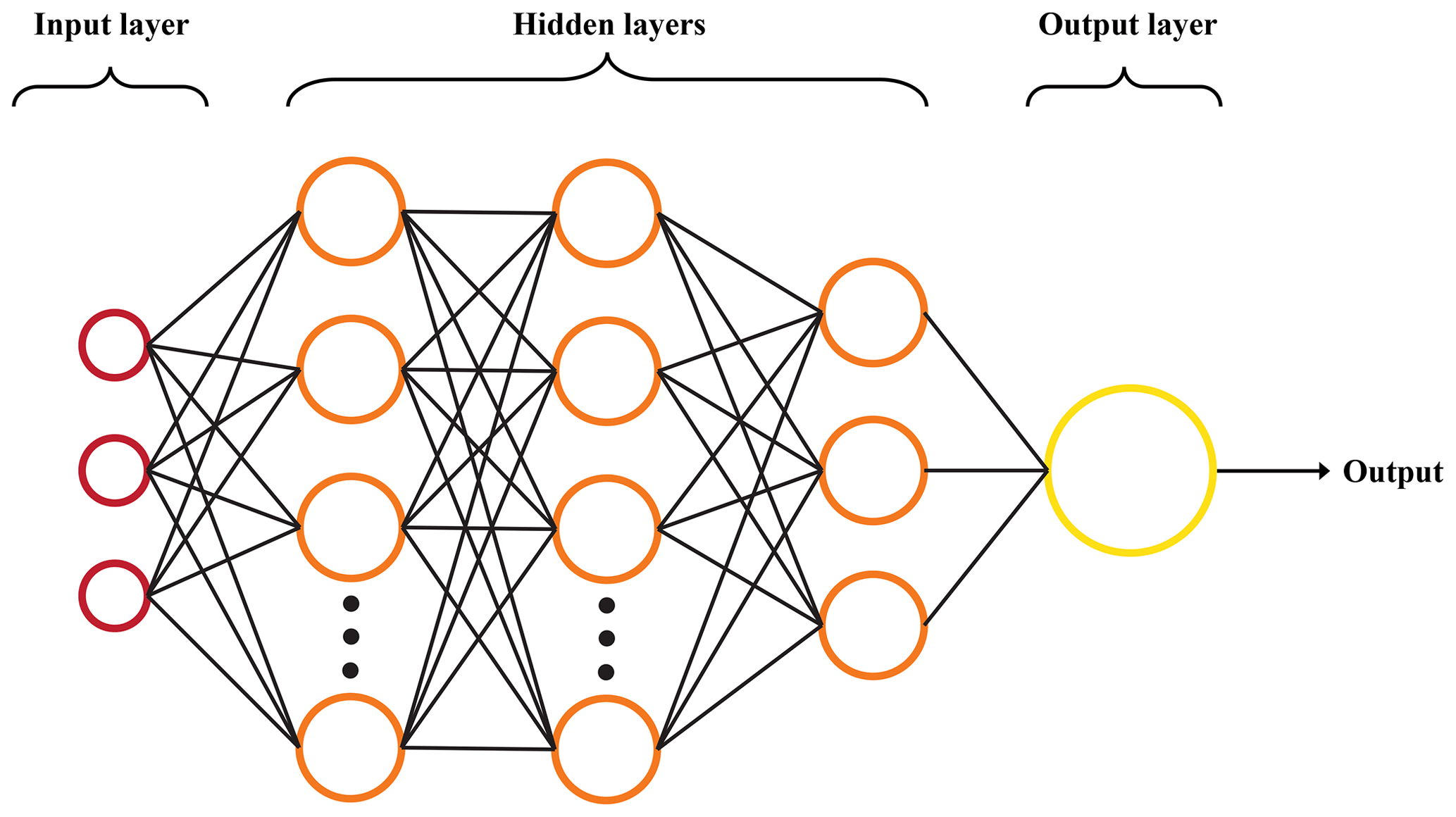
Figure 1 Artificial neural network diagram. Input nodes are in red, hidden nodes in orange, and the output node in yellow. Black lines represent weighted connections between layers.

ANNs first go through a training phase where they learn the structure of a system. Batches of training data are fed into the network, which produces an output. This output is then compared to the actual output, which is known a priori. The network then back-propagates the error through the system via stochastic gradient descent (SGD), starting from the last layer and ending at the first. During this process, the weights between layers are altered to produce a robust network physiology. This process is repeated for as many iterations as is desired, with the network seeing all training data in each iteration.

At the end of each iteration, a set of validation data is given to the network to ensure that the network is not over-fitting the training data. At the end of training, the network is given a third set of data, known as testing data, that has been unseen by the ANN theretofore. The network’s performance is characterized by its prediction accuracy on the testing data, defined by a certain error or loss metric C. This study uses the mean absolute percentage error (MAPE, Eq. 1) as the loss metric due to ease of comparison with industry metrics and its insensitivity to nondimensionalization (Appendix A).

$$\begin{array}{}\text{(1)}& C=\mathrm{MAPE}={\displaystyle \frac{\mathrm{1}}{N}}\sum _{i=\mathrm{1}}^N\mathrm{100}\times \left|{\displaystyle \frac{y_i-{\widehat{y}}_i}{y_i}}\right|,\end{array}$$

where N is the number of observations, y_i the observed output, and ${\widehat{y}}_i$ the network output. The ANN used here has a similar framework as Mohandes and Rehman (2018), containing four hidden layers with 30, 15, 10, and 5 nodes, descending until the final output layer that has a single node. Research on the effect of increasing the number of hidden layers shows that deeper networks are better able to approximate highly complex systems (Aggarwal, 2018). The number of hidden layers generally is a function of the number of input and output arguments used in the ANN as well as the perceived nonlinearity in the system. The true depth of an ANN is generally concluded based on several trial-and-error runs. Increasing the number of hidden layers in our case, however, did not yield higher extrapolation accuracy. The ANN utilized is intentionally simplistic. Potentially useful techniques such as batch normalization, recurrence, etc., are removed to further highlight the feature engineering aspect of the study. However, such additional techniques could potentially improve (or at least alter) the network's prediction accuracy and should be investigated in future studies.

There were two dropout layers, located after the first and second hidden layers, that protect against over-fitting. The activation function in each hidden layer was the hyperbolic tangent, while the output layer had a linear activation function. The MAPE cost function was utilized as the cost function C. The Adam optimization algorithm (Kingma and Ba, 2014) was implemented to enhance SGD, and all trials were discontinued after no more than 1000 iterations through the entire training dataset. All datasets were split into three distinct pieces: training data (50 %), validation data (25 %), and testing data (25 %). In order to minimize bias, all data were randomly split before each of the 10 runs for every test case. From these 10 runs, the best, average, and standard deviation of the testing data MAPE were recorded. Tests were performed with different input features and different heights at various site locations to confirm that bias from a given site and/or measurement height was removed. The Keras library, built on TensorFlow, was utilized to construct the ANN model (Abadi et al., 2016; Chollet et al., 2015).

2.2 Input features

Our main hypothesis is that more informed meteorological inputs lead to lower model extrapolation error and possibly lower error than can be achieved by existing models, especially in complex terrain. All meteorological inputs utilized in this study are listed alongside their respective definitions in Appendix B. To ensure that the model performs better than that achieved via simple analysis or with unadulterated inputs, we consider four base cases. The first is a power-law extrapolation, a simple algorithmic representation of how wind speed varies with height,

$$\begin{array}{}\text{(2)}& U_{\mathit{\alpha }}=U_{\mathrm{r}}{\left({}^z{/}_{z_{\mathrm{r}}}\right)}^{\mathit{\alpha }},\end{array}$$

where U_α is the streamwise wind speed at the height of interest, U_r the streamwise wind speed at a reference height, z the height of interest, z_r the reference height, and α a power-law coefficient that characterizes the shear between z and z_r. The α value was derived dynamically for each individual period (Shu et al., 2016). The second base case is the log-law extrapolation under neutral conditions. The formulation of the log law when the wind speed is known at a reference height can be given as

$$\begin{array}{}\text{(3)}& U_L=U_{\mathrm{r}}{\displaystyle \frac{\ln \left(\frac{(z-d)}{z_{\mathrm{0}}}\right)}{\ln \left(\frac{\left(z_{\mathrm{r}}-d\right)}{z_{\mathrm{0}}}\right)}},\end{array}$$

where U_L is the wind speed at extrapolation height, d the zero-plane displacement, and z₀ the roughness length. Both d and z₀ are determined based on optimal testing results and local topographic information (Holmes, 2018). d and z₀ are found to be 6 and 0.1 m, respectively, for the Perdigão campaign; 0 and 0.001 m, respectively, for the CASPER campaign; and 0 and 0.01 m, respectively, for the WFIP2 campaign (which are the campaigns analyzed in this study, to be discussed in Sect. 3). The log-law extrapolation (and more generally Monin–Obukhov similarity theory) is expected to perform poorly for the complex-terrain sites due to the lack of stationarity and horizontal homogeneity (Fernando et al., 2015).

The other two base cases involve using nearly raw meteorological data as input features. The third base case uses only the streamwise wind speeds (U) below the height of interest as inputs, while the fourth base case uses U, wind direction (Dir), and hour (Hr) as inputs. The hour is formatted as a cosine curve to ensure continuity between days, while the direction is formatted from $-\mathrm{1}\to \mathrm{1}$ to alleviate scaling issues.

Neural network inputs are taken at 20 m intervals to a maximum of 80 m below the height of interest (e.g., for an output at 120 m, data from 100, 80, 60, and 40 m are used). The lowest measurement height available was 40 m. Because sites (Sect. 3) had different instrumentation, the only features used are those obtained by a single profiling lidar. All lidar data are 10 min averaged. Three nondimensional features are extracted from the lidar data, namely turbulence intensity ($\mathrm{TI}{=}^{{\mathit{\sigma }}_U}{/}_U$; σ_U is the standard deviation of the wind speed), nondimensional streamwise wind speeds (U_n; nondimensionalized by U 20 m below the height of interest), and nondimensional streamwise wind speed from the previous time period (U_p). U_p is the only input feature utilized that extended up to the height of interest (i.e., we assume that the previous period's wind speed at the extrapolation height is known), and bold lettering on these three features indicates that they are nondimensional quantities. Three additional features are also extracted: vertical wind shear (dud$z{=}^{\partial U}{/}_{\partial z}$), local terrain slope in the direction of incoming flow (ϕ), and vertical wind speed (W). The nondimensional input features were selected considering their robustness in inputting more accurate features (e.g., possible compensation of measurement errors in formulating nondimensional variables) and ability of nondimensional variables to better represent flow structures (Barenblatt and Isaakovich, 1996). Features are used in various combinations in order to determine which provide useful information to the network and which provide unnecessary or redundant information that leads to confusion. All input features, many of which are highly correlated, are included in a final test to show that simply throwing multitudes of data at the network yields poor results. Including more inputs, many of which contain the same information, is not expected to improve ANN prediction accuracy because much of the additional information is redundant. Instead, the additional redundant or noisy inputs may decrease prediction accuracy because they reduce the ANN's ability to discern meaningful patterns contained in the preexisting input features.

It is typical industry practice to normalize (i.e., standardize) input variables, wherein an input variable x is scaled to $\widehat{x}$ via

$$\begin{array}{}\text{(4)}& \widehat{x}={\displaystyle \frac{x-\mathit{\mu }}{\mathit{\sigma }}},\end{array}$$

where μ is the variable's mean and σ is the variable's standard deviation (Aggarwal, 2018). This technique is particularly useful when input variables have Gaussian distributions and cover multiple scales. However, many of the input features already have similar scaling and none of the variables in our study have a Gaussian distribution, thereby drastically reducing the efficacy of standardization. Testing showed that standardization has a potentially deleterious impact on network performance (Appendix C), and therefore the input features were kept in their unaltered state. The nondimensionalization performed followed typical fluid dynamical practices (Barenblatt and Isaakovich, 1996).

The subscript 1 (e.g., U_p,1) denotes that the input value was only taken at the height of interest, subscript 2 (e.g., W₂) denotes that the input value was taken at 20 m below the height of interest, and subscript 3 (e.g., U_p,3) denotes that the input value was taken at the height of interest and 40 m below. Input variables without a subscript 1, 2, or 3 were taken from all four heights below the extrapolation height. Additionally, because a vast majority of industrial wind turbines do not produce power at exceedingly low wind speeds, all cases with streamwise velocity 20 m below the extrapolation height (U₁) <3 m s⁻¹ were removed before testing. The highest wind speed value recorded at any site was less than 23 m s⁻¹, below the standard cutoff limit of 25 m s⁻¹ (Markou and Larsen, 2009).

3 Site description and instrumentation

Data from three international field campaigns, whose locations can be seen in Fig. 2a, were used in this study. The authors participated in each of these campaigns by deployment of instruments and data analysis. The Wind Forecasting Improvement Project 2 (WFIP2) was a multiyear field campaign focused on improving the predictability of hub-height winds for wind energy applications in complex terrain (Wilczak et al., 2019). An 18-month field campaign took place in the US Pacific Northwest from October 2015 to March 2017. Several remote sensing and in situ sensors were located in a region with distributed commercial wind farms along the Columbia River basin. This study focuses on using vertical profiling lidar (Leosphere's Windcube V1) data collected by the University of Colorado at Boulder from the so-called Wasco site for a period of 15 months (Bodini et al., 2019; Lundquist, 2017). The lidar's location can be seen as the orange marker in Fig. 2b. The surrounding terrain is complex (although nominally less so than that at Perdigão to be described below), with neighboring wind farms to the east of the lidar. Any periods with missing data at multiple heights were ignored in the analysis.

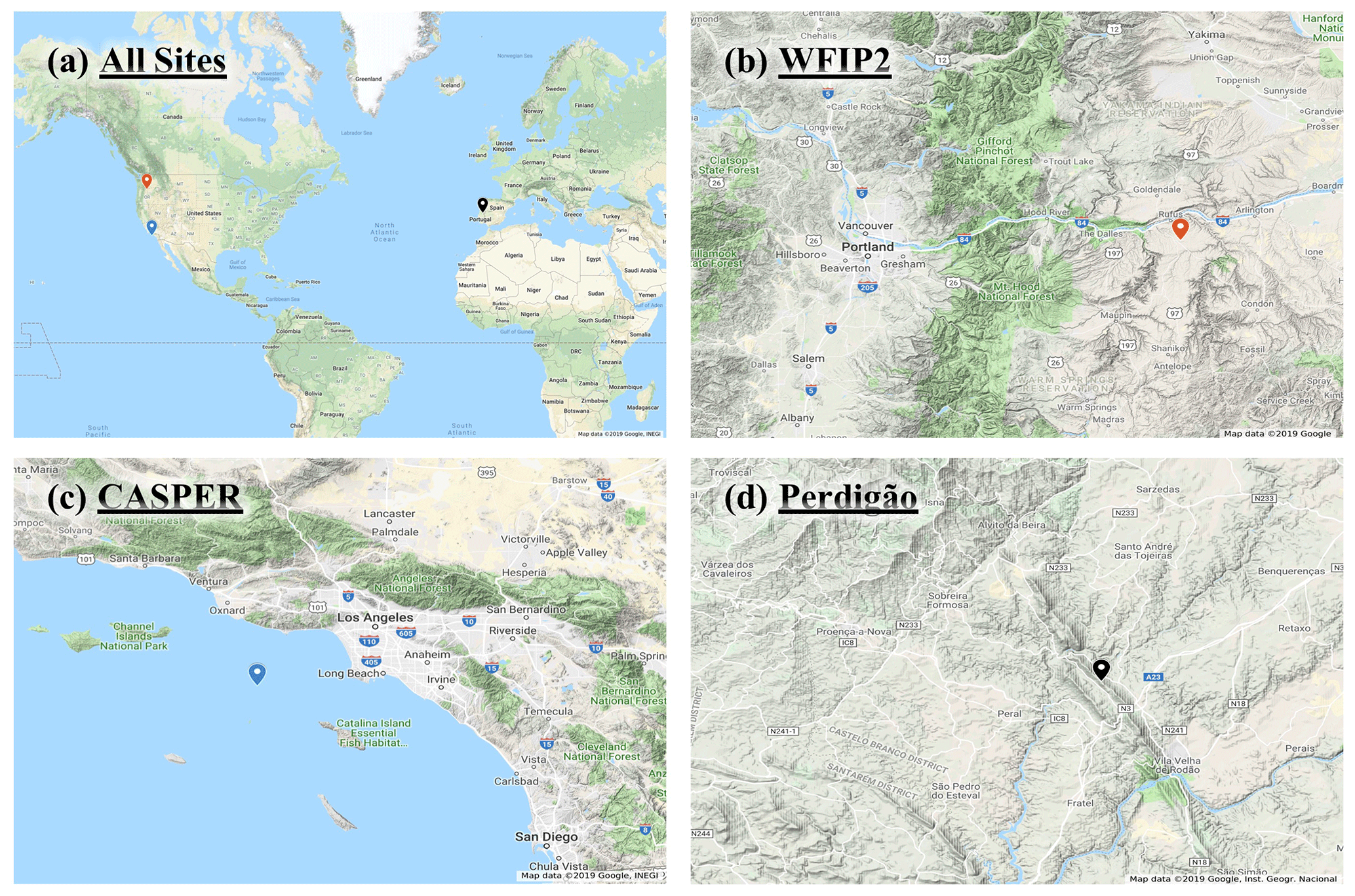
Figure 2 Panel (a) depicts all site locations. The remaining three panels depict topography at (b) WFIP2, (c) CASPER, and (d) Perdigão. Map data © 2019 Google, INEGI and Inst. Geogr. Nacional.

The Coupled Air–Sea Processes for Electromagnetic Ducting Research (CASPER) field campaign was focused on measurement and modeling of the marine atmospheric coastal boundary layer (MACBL) to better predict the interaction of electromagnetic (EM) propagation and atmospheric turbulence (Wang et al., 2018). Two field campaigns were conducted during CASPER, one near the coast of Duck, North Carolina (CASPER-East), in 2015 and another near the coast of Point Mugu, California (CASPER-West), in 2017. This study uses data from the CASPER-West experiment. Vertical profiler data (Windcube V1) from the FLoating Instrument Platform (FLIP), collected over approximately a month, were used for this study. The profiler's location can be seen as the blue marker in Fig. 2c. Datasets available at all heights were selected for this study.

The final study is the Perdigão campaign, a multinational project that took place in the spring and summer of 2017 aimed at improving microscale modeling for wind energy applications (Fernando et al., 2019). Conducted in the Castelo Branco region of Portugal, the campaign deployed an array of state-of-the-art sensors to measure wind flow features within and around a complex double-ridge topography. The ridges are spaced approximately 1.4 km apart with a valley in between. Both ridges rise approximately 250 m above the surrounding topography, which mainly consists of rolling hills and farmland. Over 4 months of data were taken from a Leosphere profiling lidar, denoted by the black marker in Fig. 2d, which was located on top of the northern ridge of the Perdigão double ridge. This particular location was selected due to the multitude of complex flow patterns seen at this location during the campaign. A meteorological tower was located adjacent to the lidar, but it only rose to 100 m above ground level, below all extrapolation heights. Profiler data available at all heights were used for this study. A manufacturer-recommended signal-to-noise ratio (SNR) threshold (−23 dB for both CASPER and Perdigão and −22 dB for WFIP2) and availability threshold (30 %) were used to remove any potentially bad data at all sites.

The uncertainty of the wind Doppler lidar measurements is expected to be within 2 % (Lundquist et al., 2015, 2017; Giyanani et al., 2015; Kim et al., 2016; Newsom et al., 2017; Newman and Clifton, 2017). Owing to a lack of secondary measurements at the locations and heights of interest, all lidar measurements are treated as true.

4 Results

Table 1 shows for each case the best testing extrapolation accuracy at all sites. The total number of (randomly split) validation and testing samples for each case is also shown for reference. The table is color coded, with the best accuracy in yellow and the worst in red. At first glance it is obvious that the network’s accuracy is highly dependent not only on the inputs used, but also on the site location and data availability. The site with the highest extrapolation accuracy is the nominally mildly complex WFIP2 site, which also has the most robust dataset. The highly complex Perdigão site has the worst extrapolation accuracy, with the accuracy of the offshore CASPER site between the two. The best MAPE achieved for all heights (underlined), with each site below 2 %, meets and often exceeds industry standards (Langreder and Jogararu, 2017).

Table 1 Best MAPE per test case. For each height at every site, the case with the best result is underlined. Yellow is the highest accuracy, and red is the lowest. The total number of validation and testing samples is shown for reference.

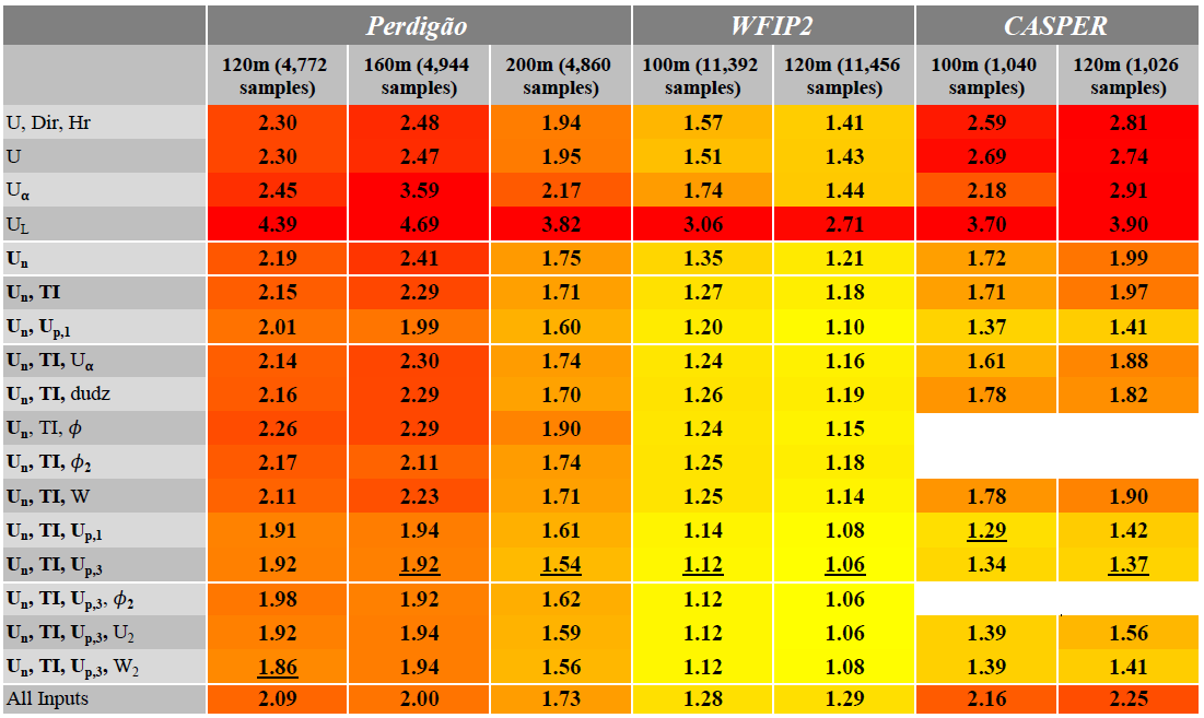
The power law performed better than the log law and was therefore used as a baseline for comparison in Table 2. As this table shows, the two ANN baseline cases (one utilizing U, Dir, and Hr, as well one only utilizing U; first two rows of Tables 1 and 2) performed almost equally well and showed a slight improvement over the power-law extrapolation. However, there is no clear distinction between the results of the two cases, and therefore Dir and Hr can be presumed to have no effect on prediction accuracy. When U is replaced by U_n, the network accuracy again improves, providing a result 10 %–33 % more accurate than the power-law extrapolation. TI and U_p,1 are the most beneficial secondary input features when used alongside U_n. While TI improves network accuracy at all except the CASPER site, U_p,1 is more impactful, improving accuracy up to 52% over the power-law extrapolation. TI was chosen as the second input for cases with three input features because it is the most beneficial feature that includes information about the flow's turbulence levels and to some extent the atmospheric stability (Wharton and Lundquist, 2012), information that is expected to be highly influential in determining the flow, particularly at the complex-terrain sites.

Table 2 ANN percent improvement over power-law extrapolation. Gold denotes the most improvement, while blue denotes less improvement or a decline in accuracy.

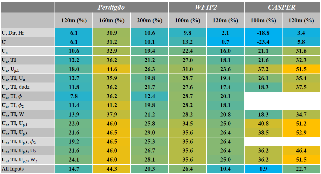
A majority of the third input features, specifically U_α, dudz, ϕ, ϕ₂, and W, have negligible or negative effects on extrapolation accuracy. There are exceptions to this rule, nevertheless, as U_α considerably improves accuracy for CASPER and ϕ₂ improves accuracy at 160 m height for Perdigão. With a single exception, the best extrapolation accuracy is obtained when U_n, TI, and either U_p,1 or U_p,3 are used as inputs. Adding extra input features beyond this point has, at best, negligible impact on network extrapolation accuracy. This is best described by the final test case where all available features are forced into the network. With all inputs, the best extrapolation accuracy is up to 67 % worse compared to the input case that obtains the best result (100 m CASPER, Table 1).

5 Discussion

A brief analysis shows that extracted nondimensional meteorological input features (U_n, TI, and U_p) drastically improve the network's extrapolation accuracy, allowing it to perform much better than conventional log-law and power-law extrapolations. However, this uptick in accuracy does not continue as more features are added. As can be seen in Fig. 3, using more than three input features for Perdigão actually reduced network accuracy. This is most obvious when all possible features are thrown into the network. The input noise and redundancy reduces the network’s ability to find usable patterns. Excess information, much of it redundant, confuses the network.

Figure 3 MAPE at Perdigão averaged over all heights. Color coding describes the number of input features used for the ANN. The dark blue bar indicates an additional test for comparison. Log-law extrapolation (4.3 % average MAPE) excluded for clarity.

Two tests were performed to determine whether this improvement in accuracy is derived from feature nondimensionalization. Because the network performed best at Perdigão with input features of U_n, TI, and U_p,3, the same inputs were then given to the network, but in dimensional form (i.e., U, σ_U, and U_p,3). The dark blue bar in Fig. 3 shows that the network performed significantly worse when given dimensional features. In fact, the network performs just as poorly with dimensional features as it does when given all the input features indiscriminately, showing that nondimensionalization has a significant impact on network performance.

Next, the 160 m Perdigão extrapolation with input features U_n, U_p,3, and TI was analyzed in depth. In order to determine the exact effects of nondimensionalization, the same inputs were then given to the network in dimensional form. The results are given in Fig. 4. The left column shows network outputs when given dimensional features, whereas the right column shows the results obtained using nondimensional features (herein referred to as the dimensional and nondimensional networks, respectively). Figure 4a and b show a comparison of true wind speed and that predicted by the network. It is immediately obvious that, upon approaching sparsely sampled regions, the dimensional network begins to fail, clearly underpredicting high wind speeds. The nondimensional network, however, does not have this problem and accurately extrapolates these higher wind speeds.

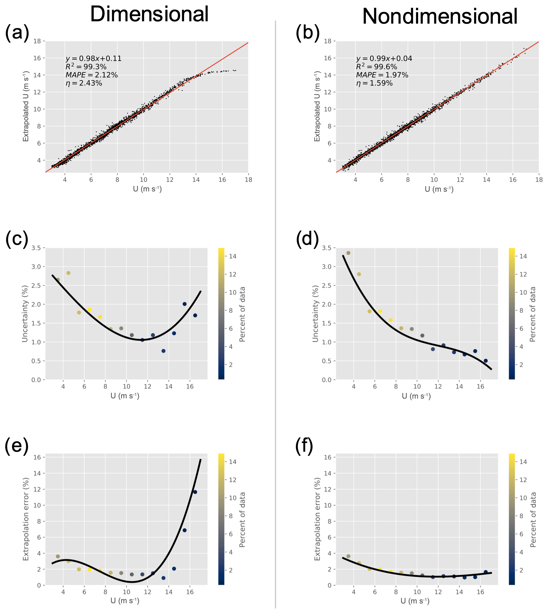
Figure 4 Comparison of network performance with dimensional (a, c, e) and nondimensional (b, d, f) input features for the 160 m extrapolation at Perdigão. The top row shows a comparison of true and extrapolated wind speed (at extrapolation height) with the best-fit line, the middle row the change in uncertainty with wind speed, and the bottom row the change in extrapolation error with wind speed. The black lines indicate a spline interpolation of the data. Colors indicate the percent of data at each binned wind speed for the testing dataset.

An elementary indicator of the network's predictive power is the coefficient of determination R², given by

$$\begin{array}{}\text{(5)}& R^{\mathrm{2}}=\mathrm{1}-{\displaystyle \frac{\sum {\left(y_i-{\widehat{y}}_i\right)}^{\mathrm{2}}}{\sum {\left(y_i-{\stackrel{\mathrm{‾}}{y}}_i\right)}^{\mathrm{2}}}},\end{array}$$

where y_i and ${\widehat{y}}_i$ have the same meanings as in Eq. (1) and $\stackrel{\mathrm{‾}}{y}$ is the mean observed output. Nondimensionalization improves R² from 99.3 % to 99.6 %. While this is a clear improvement, it does not tell the whole story. Nondimensionalization minimizes the network's dependence on wind speed, possibly by forcing it to calculate the amount of shear between reference and extrapolation heights, which is more easily determined with the assistance of TI. Therefore, it may be expected that nondimensionalization reduces error at high wind speeds where there is a deficiency of samples.

The decrease in error variance is seen in Fig. 4c and d, which show the change in uncertainty η with height. For a Gaussian variable, η can be defined as

$$\begin{array}{}\text{(6)}& \mathit{\eta }=\mathrm{100}\times {\displaystyle \frac{{\mathit{\sigma }}_{\mathit{\epsilon }}}{\stackrel{\mathrm{‾}}{U}}},\end{array}$$

where σ_ε is the standard deviation of the error (for individual predictions in the testing set) and $\stackrel{\mathrm{‾}}{U}$ the mean wind speed. For nondimensional testing, predicted wind speeds are first transformed back into the dimensional space (i.e., U_n→U) prior to error calculation in order to find true wind speed extrapolation uncertainty. The total uncertainty, a measure of error variability, is reported in the top row of Fig. 4, but the change in η with height can be seen in the figure's middle row. At low wind speeds (<4 m s⁻¹) with a large sample size the dimensional network actually outperforms the nondimensional network. As wind speeds increase, both the dimensional and nondimensional networks' uncertainties decrease at a similar rate until the sample size begins to decrease at roughly 10 m s⁻¹. At high wind speeds, the dimensional network's uncertainty begins to increase, eventually rising to almost 2 % at extrapolated wind speeds >15 m s⁻¹. The nondimensional network's uncertainty, meanwhile, continues to decrease as wind speed increases, eventually reaching values as low as 0.5 %. This is once again due to the fact that the nondimensional network is better accounting for the wind shear that is crucial for extrapolation. High wind speeds no longer appear to the network as outliers, allowing the network to better extrapolate much higher wind speeds than otherwise possible. Nondimensionalization therefore decreases output variability in sparse dimensional space, producing less volatile outputs and a more robust network.

Lastly, the change in MAPE with wind speed can be seen in Fig. 4e and f. As with uncertainty, the dimensional network's MAPE increases dramatically with wind speed due to sample sparsity. Nondimensionalization once again nearly eliminates this effect, as the MAPE consistently decreases for extrapolated wind speeds <16 m s⁻¹. Whereas the uncertainty denotes error variability, MAPE denotes overall prediction error. As is clear in Fig. 4a, the dimensional network has an obvious bias at high wind speeds, systematically underpredicting extrapolation wind speed. This is apparent in Fig. 4e, as MAPE increases to more than 10 % at higher wind speeds. The nondimensional network does not have this problem, again due to the fact that the network is oblivious to the dimensional wind speed, minimizing the prediction's dependence upon total wind speed. We therefore conclude that nondimensionalization decreases both total error and error variability in regions with a sparsity of samples by eliminating the dependence on wind speed.

CASPER is most sensitive to the choice of input features. This may be due to two factors. First, the site may have flow dynamics for which our current list of inputs cannot account (such as the Catalina eddy near the Californian Bight (Parish et al., 2013) and marine offshore internal boundary layers (Garratt, 1990) observed near that site). Additionally, it is likely that the amount of CASPER data available is not adequate for the network to accurately parse more complex hidden patterns. Fewer data could lead the network to overemphasize noisy perturbations as opposed to larger meteorological trends. It is telling that even with the small amount of data available the ANN is sometimes more than 50 % more accurate than the power-law extrapolation technique.

Although the best extrapolation accuracy occurs at WFIP2, the largest improvement over the power law is at CASPER and Perdigão. This may be due to the fact that the power-law extrapolation performed well at WFIP2 to begin with, suggesting that WFIP2 may have the simplest flow pattern of the three sites. The amount of data available did not seem to improve network performance but likely stabilized the network against noise.

We determine that of the features analyzed the nondimensional input features, U_n, U_p, and TI, most reliably help the efficacy of the ANN. Extracting the nondimensional wind speed gives the network a better idea of the general trend it needs to spot and adds more uniformity to the input samples. TI specifies the amount of turbulence and hence momentum diffusive capacity within the system (i.e., velocity gradients), a property that none of the other input features are able to directly convey. Lastly, providing the ANN with the previous period's wind speed drastically improves accuracy. This is the only feature that contains information about the flow’s history. All three of these features are important because they give the network new insightful information about evolving aspects (dynamics) of the flow.

Some of the other input features (ϕ, W, Dir) are less impactful for extrapolation, with minor effects that are site and height dependent. Adding irrelevant inputs increases the system’s noise and, unless an abundance of data are available, can cause the ANN to model coincidental or conflicting patterns. Other features (dudz, U) provide redundant information. These features typically fail to improve network accuracy, can slow the training process, and are best left out. Lastly, U_α can act as a positive or negative influence on the network because α is dependent on other parameters such as U_n, U_p, and TI. If the power-law model is reasonably accurate or has a clear repetitive bias, U_α could be a useful input feature that provides the ANN with a dependable indication of wind shear. Otherwise, it adds misleading noise to the input feature set by thwarting the steering that U_n, U_p, and TI would provide toward an accurate extrapolation.

It is obvious that just the right amount of scaled meteorological information is necessary to achieve optimal extrapolation accuracy. It is also useful to simplify the modeled system whenever possible, provided that the simplification does not remove necessary information. An example is the difference in extrapolation accuracy between U and U_n. Before the nondimensionalization, the ANN has to find a baseline wind speed and predict the vertical wind shear. With nondimensionalization, the baseline wind speed is a constant, and the network is able to exploit possible self-similarity properties of the velocity profile. Whatever information lost during nondimensionalization is more than compensated for by the improved model robustness and removal of some measurement inaccuracies, allowing for better generalization over regions in the input domain that would have a scarce amount of data (i.e., extrapolated wind speed >14 m s⁻¹).

This is only a first step in investigating how mindful feature extraction and selection can improve ANN accuracy for meteorological predictions in wind engineering. Further improvement may be possible through the addition of other meteorological elements, particularly atmospheric stability (although we expect when inputs consist of different height levels and with specification of turbulence level, the effects of stratification are indirectly taken into account). The reported list of highly beneficial atmospheric input features (U_n, U_p, and TI) is likely curtailed by our utilization of a single profiling lidar. This restraint leads to a list of atmospheric input features which are somewhat correlated, thereby reducing the predictive power of any individual meteorological input. Further instrumentation which can better capture atmospheric forcing at a larger spatial scale would likely lead to a broader, less correlated list of input features and better ANN performance. The effects of various atmospheric forcing mechanisms (atmospheric stability and inertial forcing) on atmospheric forecasting error were studied recently by the authors (Vassallo et al., 2020). Recurrent neural networks should also be utilized to test how alternative combinations of meteorological features, combined with extensive knowledge of the system's history, can improve wind speed forecasting.

6 Conclusions

Model uncertainty is a vexing problem in the wind energy industry that has vast economic implications. It has been shown that standard wind energy vertical extrapolation methods are outdated and can no longer serve their purpose of efficiently predicting and extrapolating meteorological properties accurately under various conditions (Sfyri et al., 2018; Stiperski et al., 2019). This problem can be mitigated by employing machine learning tools that have made great strides in the past few decades. Newer and faster techniques seem to spring up every few months along with a continual increase in data processing power. ANNs have the capability to delve into turbulent, nonlinear systems and may therefore be used as a tool to assist models, although blindly using ANNs without a dynamic underpinning is vacuous. Domain knowledge, especially on governing dynamical variables, can greatly assist these systems in finding underlying trends that govern atmospheric phenomena.

This study investigated the efficacy of utilizing ANNs for vertical wind speed extrapolation over a variety of terrains and evaluated how various meteorological input feature sets may influence extrapolation accuracy. Various meteorological features were combined to test their effectiveness as ANN inputs. It was found that, on average, ANN vertical extrapolation error decreases by 15 % when using U_n as a singular input feature rather that U. Two other extracted nondimensional features, TI and U_p, also led to increased extrapolation accuracy. The accuracy obtained by the ANN was up to 65 % and 53 % better than that obtained by a log-law and power-law vertical extrapolations, respectively. Vertical extrapolation error was minimized to as low as 1.06 % over 20 m, but too many network inputs (many of which are highly correlated) actually caused a reduction in network accuracy. The 160 m extrapolation at Perdigão was analyzed in depth to determine the effects of feature nondimensionalization. In addition to an improved correlation with measured wind speeds, nondimensionalization led to a decrease in both total extrapolation error and variability, particularly at high wind speeds. The nondimensional input features created a robust network that improved predictions even in rare and underrepresented cases. This shows that with sufficient data and proper feature extraction and selection, ANNs are able to improve upon the current industry standard vertical extrapolation accuracy.

Future studies are planned to investigate feature extraction and selection for wind speed predictions over a variety of timescales using a recurrent neural network. Identification of robust nondimensional variables is expected to give ANNs a better perspective of atmospheric conditions. We hope that machine learning tools, combined with proper feature selection and extraction, will reduce atmospheric model uncertainty to a fraction of what it is today.

Appendix A: MAPE magnitude invariance

Our goal is to ensure that the loss function's magnitude is invariant regardless of output scaling, allowing a fair comparison between dimensional and nondimensional networks. For a simple feed-forward neural network with j output nodes, our output error can be defined as $E=\frac{\mathrm{1}}{n}{\mathrm{\Sigma }}_c{\mathrm{\Sigma }}_j{e}_{cj}$, where c is the number of samples in a batch and e_cj is the error (given by a user-defined loss function) seen by each output node for each sample in the batch. We use the mean absolute percentage error loss function, meaning that we may define our error metric as

$$\begin{array}{}\text{(A1)}& e_{cj}=\mathrm{100}{\displaystyle \frac{\left|y_{cj}-{\widehat{y}}_{cj}\right|}{y_{cj}}},\end{array}$$

where y_cj is the true target output, ${\widehat{y}}_{cj}$ is the predicted target output, and the vertical lines denote the absolute value. For convenience consider a single sample in a single batch (this same analysis can be expanded to multiple samples over multiple batches because of the linear nature of the summation). We will refer to the true and predicted values as y and $\widehat{y}$, respectively. We can now define the true and predicted (dimensional) outputs (y_d and ${\widehat{y}}_{\mathrm{d}}$, respectively) as well as the true and predicted nondimensional outputs ($y_{\mathrm{n}}=\frac{y_{\mathrm{d}}}{a}$ and ${\widehat{y}}_{\mathrm{n}}=\frac{{\widehat{y}}_{\mathrm{d}}}{a}$, respectively, where a is a nondimensionalization variable unique to each individual case). We can find the dimensional error e_d to be

$$\begin{array}{}\text{(A2)}& e_{\mathrm{d}}=\mathrm{100}{\displaystyle \frac{\left|y_{\mathrm{d}}-{\widehat{y}}_{\mathrm{d}}\right|}{y_{\mathrm{d}}}}.\end{array}$$

Likewise, the nondimensional error e_n can be written as

$$\begin{array}{}\text{(A3)}& e_{\mathrm{n}}=\mathrm{100}{\displaystyle \frac{\left|\frac{y_{\mathrm{d}}}{a}-\frac{{\widehat{y}}_{\mathrm{d}}}{a}\right|}{\frac{y_{\mathrm{d}}}{a}}}=\mathrm{100}{\displaystyle \frac{\left|y_{\mathrm{d}}-{\widehat{y}}_{\mathrm{d}}\right|}{y_{\mathrm{d}}}},\end{array}$$

proving that the error's magnitude is invariant under nondimensionalization. This is not true for loss metrics such as mean squared error or mean absolute error, where

$$\begin{array}{}\text{(A4)}& e_{\mathrm{d}}={\left(y_{\mathrm{d}}-{\widehat{y}}_{\mathrm{d}}\right)}^{\mathrm{2}},e_{\mathrm{n}}={\displaystyle \frac{{\left(y_{\mathrm{d}}-{\widehat{y}}_{\mathrm{d}}\right)}^{\mathrm{2}}}{a^{\mathrm{2}}}}\end{array}$$

and

$$\begin{array}{}\text{(A5)}& e_{\mathrm{d}}=\left|y_{\mathrm{d}}-{\widehat{y}}_{\mathrm{d}}\right|,e_{\mathrm{n}}={\displaystyle \frac{\left|y_{\mathrm{d}}-{\widehat{y}}_{\mathrm{d}}\right|}{a}},\end{array}$$

respectively. By using the MAPE loss function, we are ensuring that the network learns at similar rates when using both dimensional and nondimensional variables.

Appendix B: Definitions of variables

Features are listed in the order that they appear in Sect. 2.2. Nondimensional features are in bold. All input variables except Hr are taken from four elevations below extrapolation height.

Uα	Extrapolated wind speed based on Eq. (2) (m s−1)
UL	Extrapolated wind speed based on Eq. (3) (m s−1)
U	Streamwise wind speed (m s−1)
Dir	Wind direction ($-\mathrm{1}\to \mathrm{1}$)
Hr	Hour of the day (cosine curve; $-\mathrm{1}\to \mathrm{1}$)
TI	Turbulence intensity; $\mathbf{TI}=\frac{{\mathit{\sigma }}_U}{U}$ (σU is the standard deviation of streamwise wind speed; both σU and U
	taken at a single elevation)
Un	Nondimensional streamwise wind speed (U at all heights divided by U 20 m below the extrapolation height)
Up	Nondimensional streamwise wind speed from the previous time period (nondimensionalized the same way as Un)
dudz	Vertical wind shear (dud$z{=}^{\partial U}{/}_{\partial z}$; s−1)
ϕ	Terrain elevation angle from direction of incoming wind speed (∘)
W	Vertical wind speed (m s−1)

Appendix C: Standardization

Standardization, while typically useful, does not improve ANN prediction accuracy in this study. To illustrate this point, consider the 120 m extrapolation at Perdigão using four distinct sets of inputs.

	Standardized	Non-standardized
U	$\widehat{U}$, $\widehat{\mathbf{TI}}$	U, TI
Un	${\widehat{\mathbf{U}}}_{\mathrm{n}}$, $\widehat{\mathbf{TI}}$	${\widehat{\mathbf{U}}}_{\mathrm{n}}$, TI

Input standardization is denoted by the caret above each input feature. By analyzing these four input feature sets we may determine network predictive performance when utilizing both standardization and nondimensionalization. U(O(1→10)) and TI(O(0.01→0.1)) are on different scales, a common issue that can reduce ANN prediction accuracy. Standardization typically alleviates this scaling problem by setting the mean value to 0 and the variance to 1 (Eq. 4), but because neither distribution is Gaussian (both have large positive tails) standardization is not a viable solution to this problem. ANN prediction results for a typical run can be seen in Fig. C1. It may be determined from these results (which are illustrative of those seen across a variety of input feature sets) that standardization, rather than improving ANN predictive accuracy, actually confuses the network. For this reason standardization was excluded from the investigation.

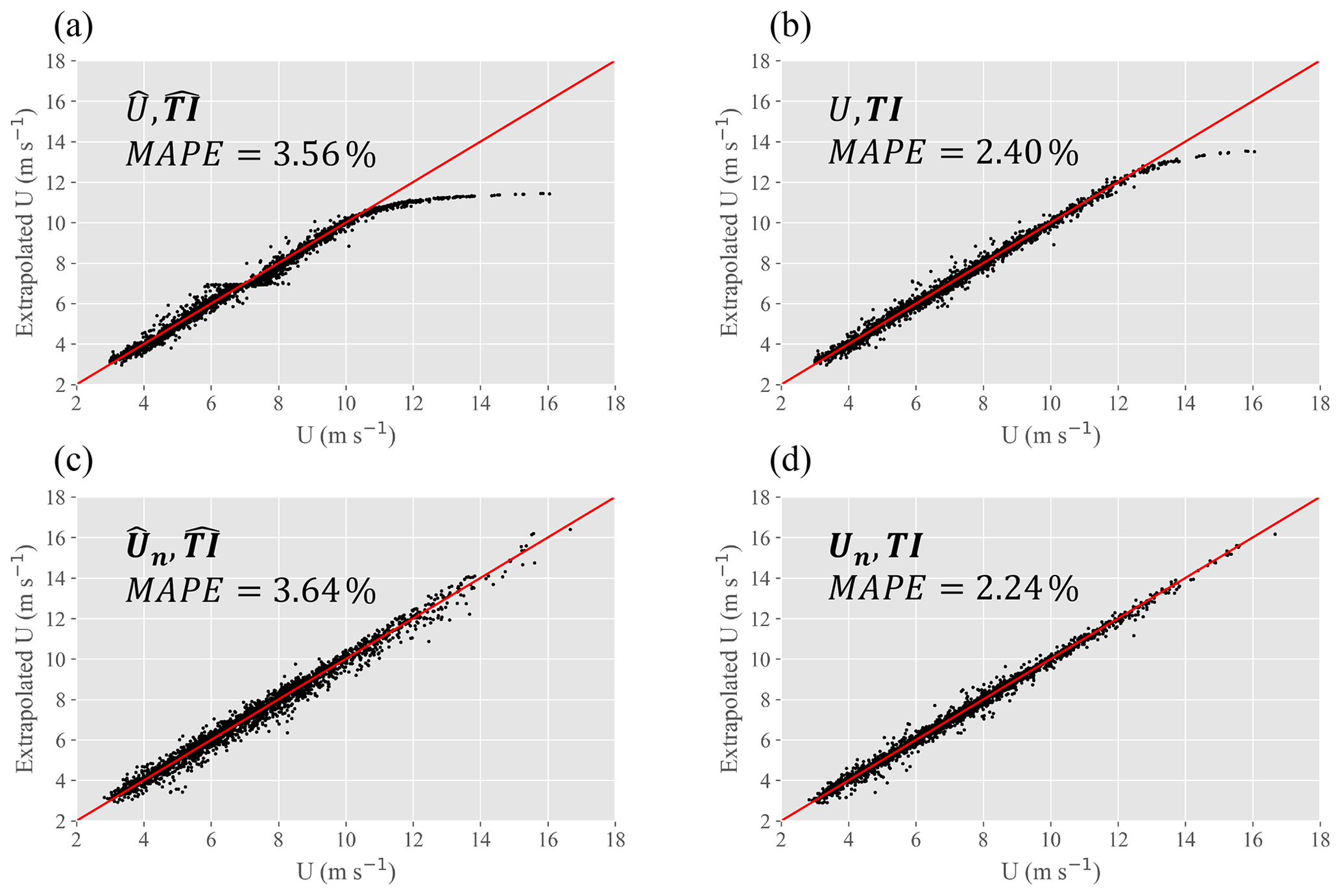
Figure C1 Comparison of test results using standardization and nondimensionalization (for U) preprocessing techniques. Standardization (a, c) can be seen to reduce prediction accuracy, whereas transformation of U to U_n (U shown in a and b, U_n in c and d) can be seen to improve predictive accuracy by removing the tailing effect at high wind speeds.