the Creative Commons Attribution 4.0 License.
the Creative Commons Attribution 4.0 License.
 | 19 Jan 2021
Characterisation of intra-hourly wind power ramps at the wind farm scale and associated processes
Mathieu Pichault
Claire Vincent
Grant Skidmore
Jason Monty
One of the main factors contributing to wind power forecast inaccuracies is the occurrence of large changes in wind power output over a short amount of time, also called “ramp events”. In this paper, we assess the behaviour and causality of 1183 ramp events at a large wind farm site located in Victoria (southeast Australia). We address the relative importance of primary engineering and meteorological processes inducing ramps through an automatic ramp categorisation scheme. Ramp features such as ramp amplitude, shape, diurnal cycle and seasonality are further discussed, and several case studies are presented. It is shown that ramps at the study site are mostly associated with frontal activity (46 %) and that wind power fluctuations tend to plateau before and after the ramps. The research further demonstrates the wide range of temporal scales and behaviours inherent to intra-hourly wind power ramps at the wind farm scale.
- Article
(7164 KB) - Full-text XML
- BibTeX
- EndNote


Environmental protection and sustainability have become the main incentives to integrate more green energy sources into electrical systems. Numerous countries are currently moving towards greener energy production sources to achieve the Paris Agreement's goal to keep global warming below +2∘ by 2100 (UNFCCC, 2015). Since the early 2000s, wind energy has gained significant traction and is currently the fastest-growing mode of electricity production across the globe (EIA, 2019), with up to 51.3 GW of wind power capacity installed worldwide in the year 2018 alone (GWEC, 2019). In emerging markets such as Australia, Canada and the United States, newly built wind farms are installed in large blocks, often exceeding 400 MW (Kariniotakis, 2017). With ever-growing wind penetration in the grid, electricity networks are increasingly subject to fluctuations in power production. These fluctuations are called “ramp events”, referring to the sudden variations in wind power generation over a short period of time. Motivated by the need to enhance management of such events as well as by optimising integration and control of wind farms, there is currently a great incentive to develop accurate and timely short-term (intra-hourly) ramp forecasts (Zhang et al., 2017; Cui et al., 2015; Gallego et al., 2015a).
Sharp increases (“ramp-up”) or decreases (“ramp-down”) in wind power generation over a short period of time give rise to both financial and physical impacts. First, wind power ramps are a risk to electric system stability and their mismanagement can have dramatic consequences, such as power outages (Tayal, 2017; Trombe et al., 2012). These can be particularly detrimental to electrical networks located in areas with a low degree of inter-connectivity (i.e. remote regions or islands), where significant power variations are not easily balanced (van Kooten, 2010; Treinish and Treinish, 2013). Both ramp-ups and ramp-downs can exhibit diverse levels of severity (i.e. likelihood to cause disturbances) according to the time and geographic scale over which the ramp occurs (Zhang et al., 2014). However, ramp-downs are generally considered more likely to impact grid system stability due to the limited availability of reserve power (Zhang et al., 2017; Jørgensen and Mohrlen, 2008). Additionally, wind farms are often curtailed during ramp-ups as electricity surplus cannot be dispatched, which represents loss of potential profits for wind farm owners. In many cases, wind farm owners also have to cover additional costs when they are unable to meet specific loads and quotas.
Improved ramp prediction can help mitigate the issues listed above. However, wind power ramps are particularly challenging to predict. This is partly due to the wide variety of timescales over which they occur, ranging from a few minutes up to several hours (Worsnop et al., 2018). At the wind farm scale, numerical weather prediction models struggle with forecasting wind power fluctuations occurring within an hour and often fail to predict accurately the timing and the amplitude of the ramps (Zack et al., 2011; Magerman, 2014). In practice, the vast majority of operational short-term wind forecasts rely primarily on variations of the persistence method (or “naive predictor”) (Wurth et al., 2018), which assumes that there will be no variation between the current conditions and the conditions at the time of the forecast. Persistence forecasts inherently tend to perform poorly during ramp events.
Wind power ramps are usually characterised by their magnitude ΔP, duration Δt, rate ΔP∕Δt, timing t0 (central time or starting time of the event) and gradient (ramp-up or ramp-down) (Sherry and Rival, 2015; Lange et al., 2010; Ferreira et al., 2010). However, defining a ramp event is a non-trivial task. In fact, there is currently no commonly agreed upon definition for a wind power ramp (Gallego et al., 2015a; Mishra et al., 2017) as its interpretation can vary substantially between applications (Wurth et al., 2019; Cutler et al., 2007; Bradford et al., 2010; Greaves et al., 2009). In addition, some operators may need to evaluate the likelihood of ramps occurring based on various definitions simultaneously (Bianco et al., 2016). Many wind power ramp studies employ a binary, threshold-crossing identification system. However, these binary identification systems are limited by the high sensitivity of the definition to the adopted threshold. Furthermore, it implies all ramps are identical and does not provide further insights into their severity. To alleviate these shortcomings, the so-called “ramp functions” have been introduced, which provide an estimation of the ramp intensity at each time step. Gallego et al. (2013, 2014) first introduced a ramp function based on a continuous wavelet transform (the “Haar” wavelet) of a wind power time series, and Martínez-Arellano et al. (2014) proposed a ramp function based on a fuzzy-logic approach to characterise ramps for the day-ahead market. More recently, a continuous wavelet transform (CWT) based on a Gaussian wavelet was used by Hannesdóttir and Kelly (2019).
A precursor to successful ramp predictions is a sound understanding of the conditions under which ramps occur (Couto et al., 2015). Identifying the temporal and spatial scales pertaining to ramps also provides valuable insights into the limits of numerical weather prediction models and associated uncertainties (Gallego et al., 2015a). Nonetheless, ramping behaviour analysis is a relatively new research field and very little is known about the main processes inducing ramps (Mishra et al., 2017). In Cutler (2009), approximately 40 % of the ramps observed at three Australian wind farms were associated with frontal systems, while neighbouring high- and low-pressure systems and troughs accounted for 35 % of the ramps. In Jørgensen and Mohrlen (2008) and Sherry and Rival (2015), the authors observed a strong correlation between ramp events and chinook (föhn) wind days, emphasising the importance of local meteorological events in forming ramps. Deppe et al. (2012) found the presence of low-level jets was the primary driver of ramps at a site located in Pomeroy (IA, USA). Other studies in central Europe have shown that most critical ramps arise from extreme weather events such as cyclones (Steiner et al., 2017; Lacerda et al., 2017). These findings suggest a relatively high degree of association between ramping behaviour and large-scale atmospheric circulation processes, emphasising the great potential to use synoptic-scale forecasts and operational decision tools to support power systems with a high degree of wind penetration. Although discussed in multiple studies (Deppe et al., 2012; Ferreira et al., 2012; Freedman et al., 2008; Kamath, 2010; Sherry and Rival, 2015), there is no consensus in the literature on seasonal and diurnal ramp patterns, underlining the influence of local features on ramping behaviour. In summary, we see that the expected main drivers of ramps can vary significantly according to geographic location and that site-specific conditions such as terrain roughness, orography and air–sea–land interactions play a critical role in inducing ramps at the wind farm scale.
As pointed out by Cutler et al. (2007), Gallego et al. (2013, 2015b) and Mishra et al. (2017), robust ramp classifications are still currently needed owing to the emerging nature of the subject. Review of the literature revealed that while studies assessing the causality of wind power ramps exist, these focus mostly on a limited number of critical events rather than on more frequent fluctuations. The lack of clear identification criteria prevents the implementation of automatic classification schemes and hence precludes tracing the causality of more common (less severe) ramps. Hence, it is of both scientific and practical interest to develop automatic schemes for (intra-hourly) ramp categorisation. This study aims at characterising intra-hourly wind power ramps and their underlying processes at the wind farm scale through such an approach. The paper is organised as follows. The methodology to detect ramps and extract relevant features, as well as to categorise ramps according to their underlying processes, is established in Sect. 2. Section 3.1 provides details on the main ramp features at the study site. Section 3.2 addresses the underlying meteorological and engineering causes of ramps, and ramp shapes are discussed in Sect. 3.3. For illustrative purposes, characteristic case studies are presented in Sect. 3.4. Finally, conclusions and a discussion of future works are presented in Sect. 4.
2.1 Data
Data were collected at the Mount Mercer wind farm (“the site”) in Western Victoria (southeastern Australia). The site is comprised of a 2650 ha area of moderately complex topography. The prevailing wind direction at the site is north-northwest, with occasional westerly and southeasterly winds. A total of 64 identical doubly fed induction generator wind turbines manufactured by Senvion (model MM92) of 2.05 MW nominal rated capacity are installed on-site, corresponding to a total installed capacity of 131.2 MW. The power curve characteristic of the wind turbines is presented in Fig. 1. The wind turbines are expected to reach their rated capacity for wind speed above 11 m s−1. The cut-in speed of the wind turbines is 3 m s−1.
All data analysed as part of this study were collected between 1 October 2016 and 1 March 2019. Power data consist of 1 min averaged total power generation of the wind park. Outliers and periods of abnormal operation were filtered out of the power generation time series. Wind data collected at the site as part of this assessment include 1 s resolution (1 Hz) wind speed and wind direction measurement. Wind data originate from two 80 m high meteorological towers (“met masts”), MM1 and MM2, each of them comprising two cup anemometers installed at 78 and 80 m above ground level () and two wind vanes installed at 35 and 76 . Likewise, pressure, temperature, and relative humidity data are collected on both met masts at 76 . The density of moist air is derived from these measurements using the ideal gas law and Dalton's law of partial pressures. MM1 and MM2 are located in the northwest and southeast corner of the site, respectively. Figure 2 shows the layout of the wind farm along with the location of the turbines and met masts.
The area surrounding each met mast contains several turbines that have been considered according to the standard IEC (2005). The resulting sector free of wake effect is [290∘, 110∘] for MM1 (measured clockwise from true north) and [79∘, 259∘] for MM2, and all wind data from sectors outside these ranges were removed from the data set (the valid data from the two met masts are combined to create an almost complete circle).
As no rain gauge was installed on-site at the time of the study, precipitation data required for the ramp classification scheme were collected from the Australian Bureau of Meteorology Sheoaks weather station (BOM, 2020a), located approximately 25 km southeast of the site (lat −37.910000, long 144.130000). We note here that precipitation measurements from the meteorological station do not necessarily reflect on-site conditions, especially for rain events with short spatial and temporal scales. As a result, using off-site data to characterise on-site conditions can, in some cases, be ill-founded. This is flagged as a limitation of the study and taken into account in the design of the ramp classification scheme (see Sect. 2.3).
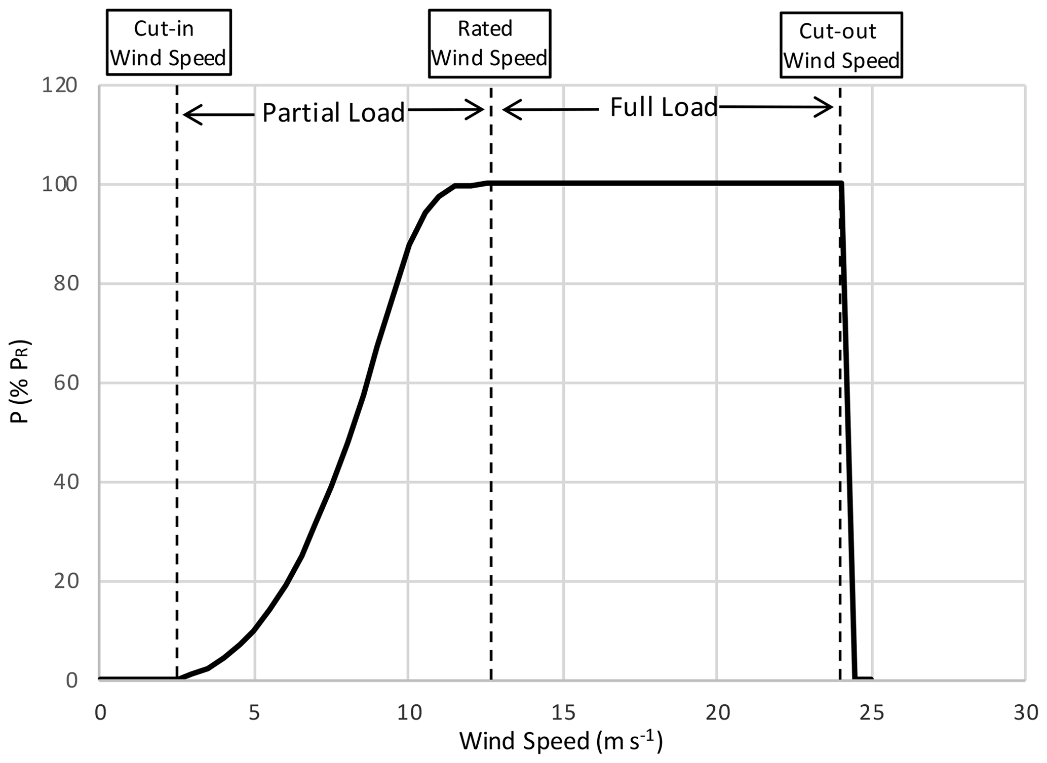
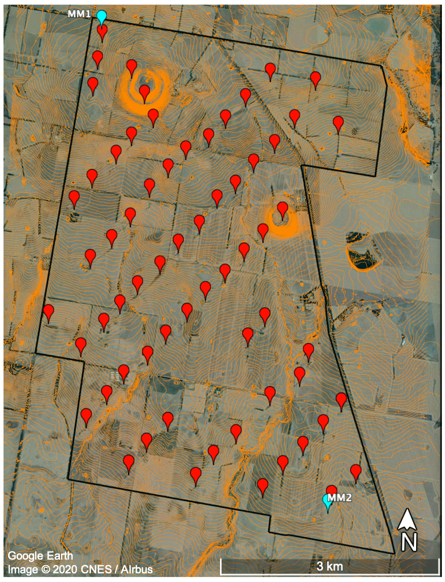
Figure 2Layout of the Mount Mercer wind farm (background map data: © Google Earth, CNES/Airbus). The location of the 64 turbines and the 2 met masts are designated by the red and blue markers, respectively.
2.2 Ramp function
Ramps typically correspond to sudden localised changes in a wind power time series. It is possible to characterise ramps based on the notion that ramps occur when a specific large gradient is maintained during successive time steps in a wind power time series through so-called ramp functions. The main focus of ramp functions is to provide an estimation of the intensity of the ramp at each time step of a wind power time series.
Wavelet analysis has shown to be a powerful tool to study variations in local averages (Percival and Walden, 2000). CWT has been used in the wind energy space to characterise wind power ramps (Gallego et al., 2013, 2014) and wind speed ramps (Hannesdóttir and Kelly, 2019). The continuous wavelet transform (CWT) enables decomposition of a time–amplitude signal in the time–frequency domain and hence provides information on the timing t′ and the scale γ of particular events. Briefly stated, the CWT is obtained by computing the product between a signal pt and a mother wavelet Ψ(t) which has been transformed through shifting and stretching operations:
where Wp values are the wavelet transform coefficients, which are functions of the scale dilatation γ and time shift t′.
In the context of this study, a ramp function following the procedure outlined by Gallego et al. (2013) was implemented. For the sake of completeness, the methods and equations as per Gallego et al. (2013) are presented in the remainder of this section. The approach is based on the CWT of the Haar wavelet to provide an estimation of the ramp intensity at each time step. Amongst the numerous existing wavelet forms, the Haar wavelet was chosen for the adopted methodology because of its capacity to quantify the gradient of a signal at various timescales (Percival and Walden, 2000). The coefficients resulting from the CWT based on the Haar wavelet transform of a wind power time series pt are denoted Wp(t, γ) and expressed by
Note that the coefficients described in Eq. (2) are derived from the additive inverse of the conventional Haar wavelet (obtained by changing the sign of the mother wavelet). This was done so as to obtain coefficients whose signs are equal to the sign of the gradient experienced by the time series. The ramp function Rt is then defined as the sum of each CWT coefficient calculated for the scale interval [γ1, γN]:
The ramp function (or “ramp score”) is considered a reflection of the ramp intensity as the contribution to the gradient is assessed for different scales at each time step. The ramp function defined by Eq. (3) can be normalised by its maximum absolute value to generate the normalised ramp function Rnorm t, which is between 1 (the strongest ramp-up) and −1 (the strongest ramp-down).
2.3 Ramp detection and characterisation
First, a wavelet-based ramp function (Gallego et al., 2013) is computed to quantify the ramp performance (or “score”) at each time step of the time series. The ramp function is computed on the time series using a scale range [γ1, γN] of [2,60], therefore primarily targeting ramps occurring over a maximum time window of 60 min (intra-hourly ramps). Times t′ of the most significant ramps are identified by selecting the 1 % of events associated with the strongest absolute ramp intensity (i.e. times associated with the highest ramp scores). The maximum wavelet coefficient at the timing of the ramp determines the timescale γ (or “scale”) of the ramp. The approach which consists of identifying ramps' timescales based on the maximum wavelet coefficient was first implemented in a study by Hannesdóttir and Kelly (2019), in which ramps in wind speed are studied. The subset of the wind power time series of length γ and centred on t′ will henceforth be referred to as “the ramp”.
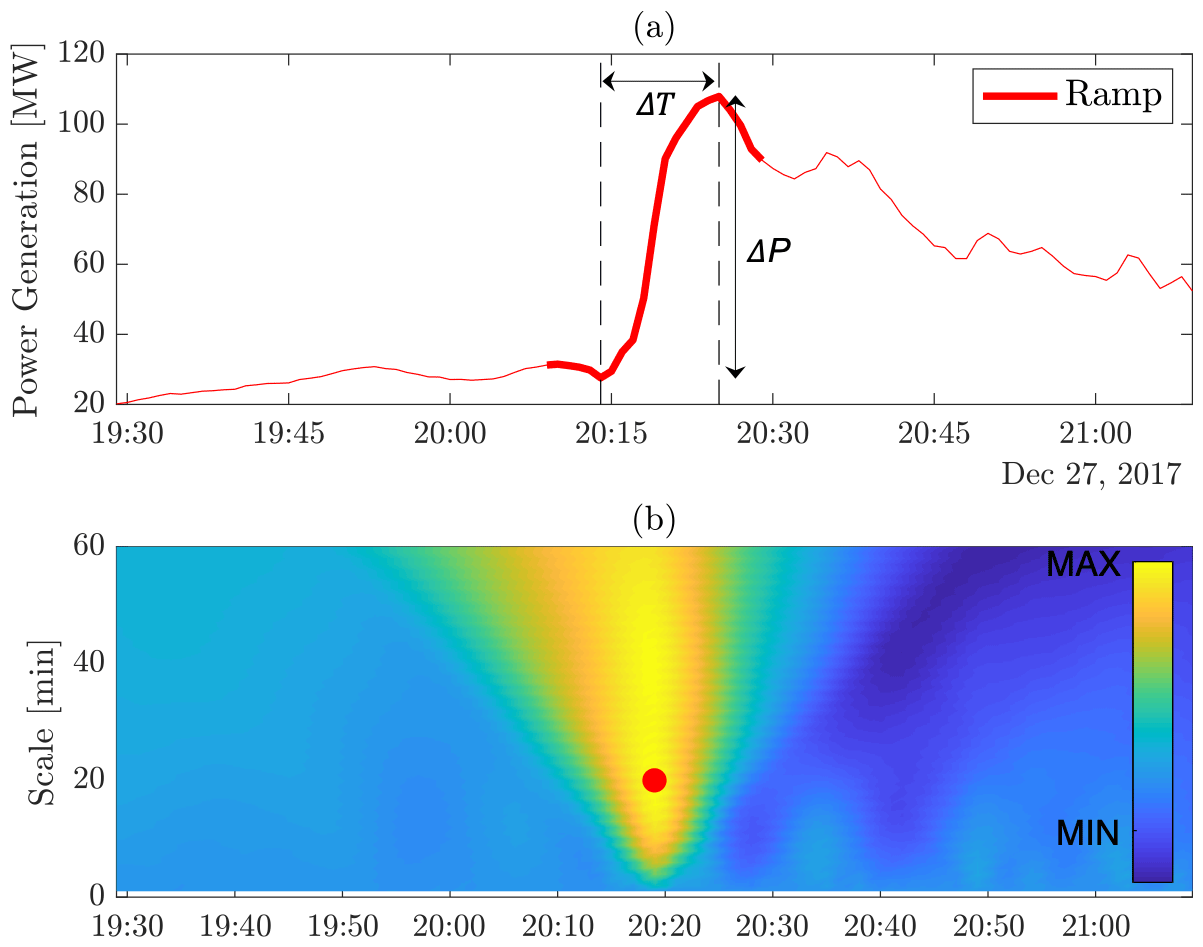
Figure 3(a) Power generation time series surrounding ramp rank ID number 5 and (b) coefficients of its continuous wavelet transform based on the Haar wavelet. The ramp timing (central point of the ramp) is on 27 December 2017 at 20:19 UTC+10. The thickened red line in (a) represents the ramp, whose amplitude ΔP is 65 MW and rise time ΔT is 11 min. The red dot in (b) indicates the maximum coefficient at the timing of the ramp, corresponding to a scale γ of 20 min.
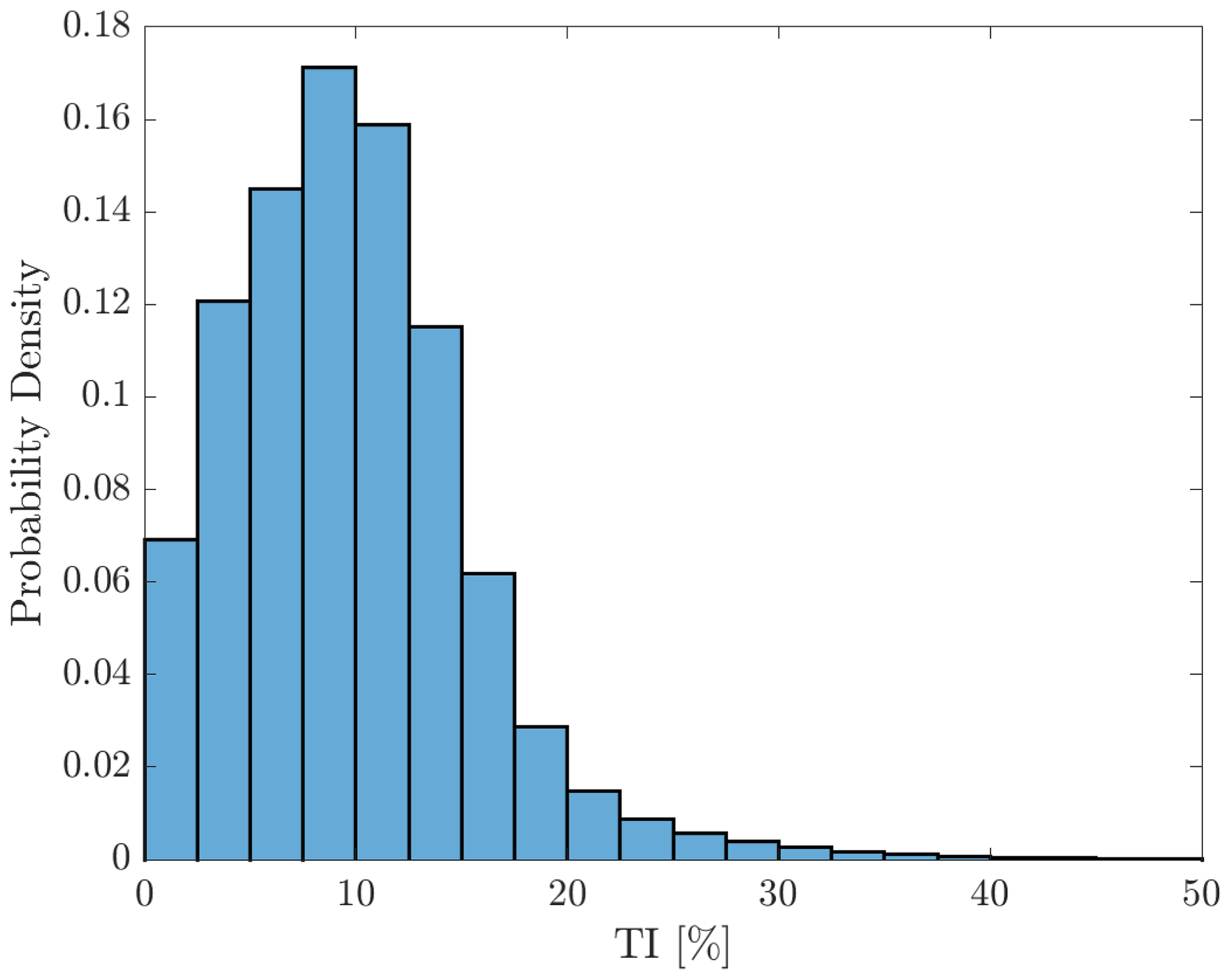
Figure 4Frequency distribution of turbulence intensity at the Mount Mercer wind farm between 1 October 2016 and 1 March 2019.

Figure 5Schematic of the decision tree of ramp-associated meteorological and engineering drivers.
Finally, two ramp features, namely the ramp amplitude and the rise time, are retrieved. The ramp amplitude, denoted ΔP, is defined as the maximum power variation over the subset length γ centred on t′. The rise time hereafter refers to the elapsed time between the lowest and highest power level during the ramp.
Figure 3 illustrates the decomposition of a wind power generation time series into its wavelet coefficients. The thickened red line on Fig. 3a represents the ramp of the scale γ=20 min, and the vertical and horizontal arrows indicate the amplitude (65 MW) and the rise time (11 min), respectively. The red dot on Fig. 3b displays the highest absolute coefficient value at the timing of the ramp, which corresponds to a scale γ of 20 min. Note that the longest ramp scale to be identified through this method is 60 min since the ramp function is calculated with an upper scale range limit γmax of 60.
In order to avoid ramp over-identification (i.e. identifying variations of the same event multiple times), ramps associated with a lower score occurring within the scale range of a more significant ramp are discarded. Based on the methodology above, a total of 1183 ramps are identified in the 29-month period.
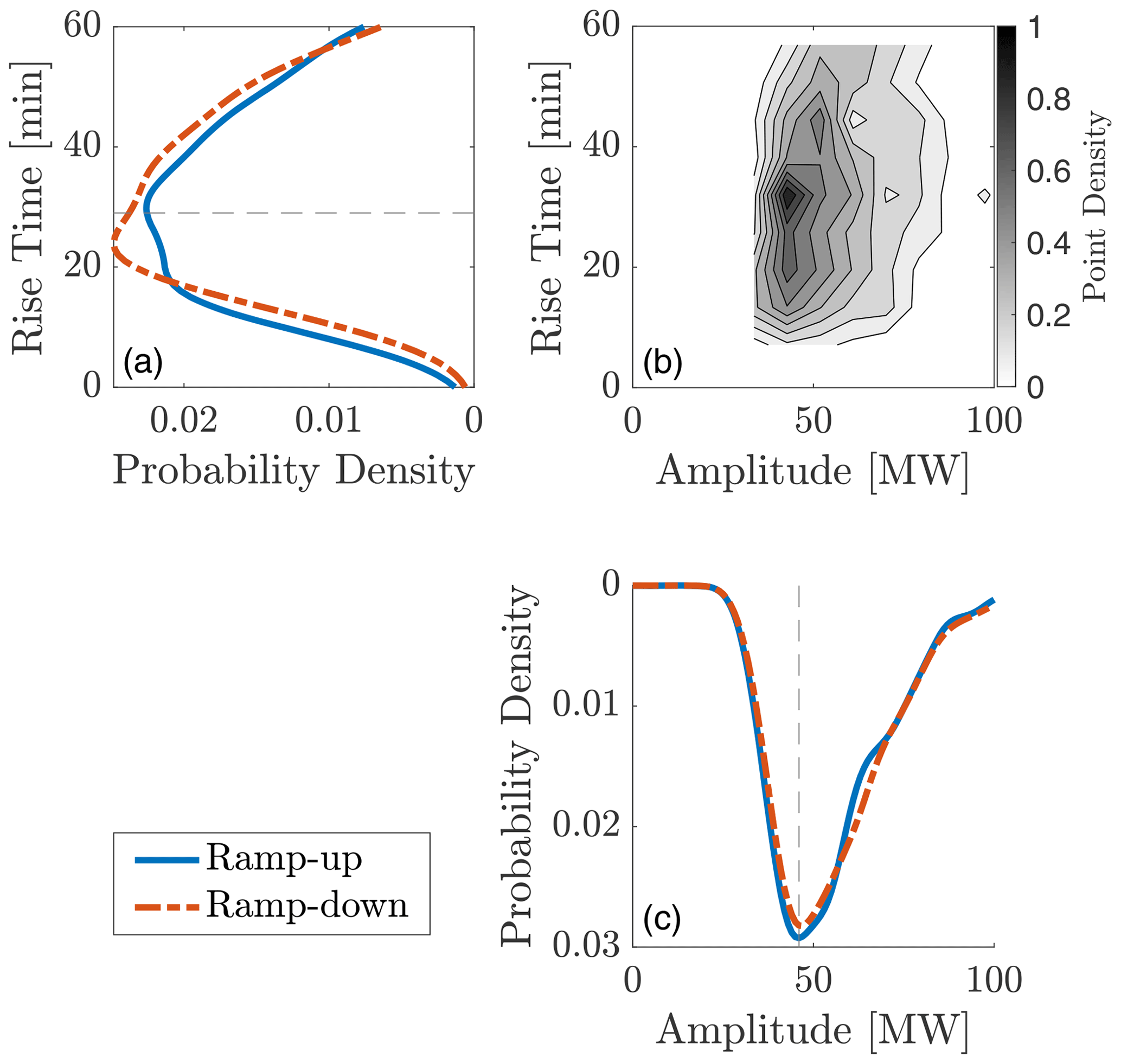
Figure 6Joint probability density distribution of the ramp amplitude and rise time (b) and associated univariate probability density distributions for ramp-ups and ramp-downs (a, c). The dashed lines display the mode of the combined distributions.
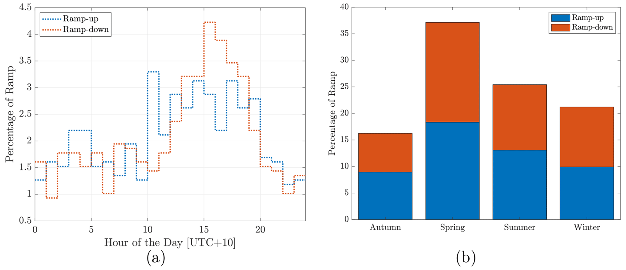
Figure 7(a) Hourly ramp distribution and (b) bar plot of the seasonality of the ramps, based on data from between 1 January 2017 and 1 January 2019.
2.4 Ramp categorisation
In this section, we present the automatic scheme developed to classify ramps according to their underlying causes. While it is expected that processes associated with ramps will present common structural features, their realisations are, in essence, unique and might involve a range of factors. Therefore, the goal here is to identify the most likely ramp driver as opposed to capturing every possible scenario that could have resulted in a ramp. The method is designed to automate ramp classification based on easily accessible data. The data set of ramps to be classified excludes ramps occurring during periods of environmental-sensor failure, identified by constant readings. The filtering process effectively removed eight ramps from the original data set. For the sake of clarity, a decision tree used to diagnose ramp driver categories is summarised in Fig. 5. Based on the review of the literature on ramp drivers, we established criteria to classify ramps into six categories. The criteria are as follows (by order of priority).
-
Passage of a front. Weather fronts are caused by abrupt changes in air mass and are often associated with strong low-altitude winds, precipitation and a shift in wind direction. Such macro-scale meteorological processes often incur large wind power generation fluctuations (increase caused by the passage of the front and decrease caused by the pre-frontal lull or post-frontal relaxation). The criterion to identify fronts is adapted from the Melbourne Frontal Tracking Scheme (Simmonds et al., 2012), initially developed to explore cold-front behaviour in the Southern Hemisphere from reanalysis data. The method was selected by the authors amongst numerous objective algorithms due to its ability to identify fronts in the Southern Hemisphere with remarkable accuracy while preserving a straightforward, easily understandable scheme. The front identification scheme is summarised as follows: (1) the sign of the meridional component of the wind (v) changes from positive to negative over successive time points [t, (t+6 h)] (i.e. the wind direction shifts from the southwest to the northwest quadrant), and (2) the amplitude change in the meridional wind component is larger than 2 m s−1 over the same 6 h interval. As the method was originally developed for the ERA-Interim reanalysis (Dee et al., 2011) on a 1.5∘ latitude–longitude (approx. 160 km) grid, the objective function was further adapted to process data from discrete spatial points by applying a 4 h moving-average filter to the wind data time series. The use of such an averaging window is justified by the fact that spatial averaging over a 160 km grid is somewhat equivalent to temporal averaging over approximately 4 h, assuming an average wind speed during ramps of 11 m s−1. Additionally, computing the adapted front detection algorithm using a 4 h averaging window provided high agreement with front identification through inspection of mean sea-level pressure (MSLP) charts. In short, the objective scheme for ramps associated with frontal passages is a wind shift from the southwest to the northwest quadrant combined with a change in meridional wind greater than 2 m s−1 when comparing wind conditions with a 4 h moving average 3 h before and after the ramp timing. The reader interested in implementing a similar automatic front scheme targeting the Northern Hemisphere is referred to Bitsa et al. (2019).
-
Post-frontal activity. To capture the strongly variable wind conditions following the passage of a front, where cold-air outbreaks and cellular convection often dominate the flow fields, ramps occurring within 12 h of the passage of a cold front but not related to the front itself were labelled as post-frontal driven. The adapted front identification scheme introduced above was applied to the entire wind time series with an hourly time step. If more than one front was detected over successive time steps, the most likely front timing was selected with the local maximum of the cumulative sum over a 6 h window. A total of 394 fronts were identified following this methodology, which corresponds to a front occurring approximately 2 % of the time within the time series.
-
Non-frontal precipitation. Precipitation not associated with a front can also induce wind speed variations through processes including convective downdrafts, mesoscale circulations or microbursts (e.g. Fournier and Haerter, 2019; Potter and Hernandez, 2017). The gustiness can be organised as a gust front or cold pool with potential to propagate through a wind farm, which has been considered by Potter and Hernandez (2017) in the context of fire weather. After classifying frontal and post-frontally associated ramps, the remaining ramps where at least 1 mm of cumulative precipitation is recorded within a 2 h window centred on the ramp are defined as non-frontal precipitation ramps. The 2 h timescale is chosen conservatively to allow for propagation time between Sheoaks station and the site and vice versa. A limitation of this method is that both convective and stratiform precipitation will be included. A full exploration of the role of gust fronts and convective downdrafts on wind power predictability is outside the scope of this study.
-
Large change in turbulence intensity. Another kind of atmospheric process that can potentially cause ramps is associated with vertical-momentum-flux changes affecting the structure of the atmospheric boundary layer. We suggest two ways in which a change in vertical turbulent mixing can induce wind power ramps. First, ramp-up events can occur in the instance of a high-wind-speed layer situated above hub height in conjunction with the erosion of a stable boundary layer. The second method is where rapid radiative cooling of the surface layers can result in a substantial increase in thermal stability, hence reducing vertical momentum flux and wind power harvested at hub height. Albeit to a lesser extent, a decrease in the turbulence intensity level may also influence the potential development of wakes, low-level jets and gravity waves, although the diagnosis of these effects is outside the scope of this study. To identify ramps associated with sudden shifts in vertical momentum flux, we used a criterion based on turbulence intensity (TI) at hub height. After removing the linear trends from each of the 10 min long segments, we computed the horizontal turbulence intensity from the on-site cup anemometers: , where σU [m s−1] and [m s−1] are the average standard deviation of the horizontal wind speed and the average horizontal wind speed over a 10 min period, respectively. Recall that only wind data from undisturbed wind direction sectors (not in the wake of neighbouring wind turbines) were included in the assessment. In this study, we relate ramps to large TI changes when the amplitude of TI (difference between maximum and minimum) throughout the ramp exceeds a conservative threshold of 10 %. For reference, the TI distribution observed at the site during the assessment period is shown in Fig. 4.
-
Shutdown cases. Small changes in wind speed can have a significant impact on power production when velocities are close to the wind turbines' cut-out wind speed (wind speed above which the turbine will automatically shut down for safety reasons). Hence, ramps were labelled as shutdown situations when the maximum 10 min averaged wind speed measured at the site exceeded the cut-out wind speed (24 m s−1) during the ramp. This criterion is based on the cut-out strategy as outlined in the on-site turbines’ datasheet.
-
Non-linearity of the power curve. Although sudden changes in wind speed usually cause significant power variations, minor variations in a moderate wind regime can also lead to substantial wind power fluctuation. This is due to the non-linear relationship between wind speed and power generation, shown in Fig. 1. Non-linearity of the power curve is not a driver of its own, but this ramp class aims to complement previously introduced drivers and as such will be considered separately. Ramps are associated with the non-linear wind-to-power conversion processes when the amplitude in 10 min averaged wind speed is less than 3 m s−1 and comprised within the 5–10 m s−1 window (i.e. the steep portion of the power curve).
2.5 Ramp shape
As part of the ramp characterisation, the overall shapes of the power fluctuations encompassing ramps were investigated, with a view to answering the question of whether particular ramp drivers have a characteristic ramp shape. A subset of the power generation time series is extracted for each ramp identified above. The subset is centred on the ramp timing t′ and is of duration equal to three rise times (3ΔT). The wind power subset with a duration of three scales and centred on the ramp timing will be hereafter referred to as the “extended ramp”. To compare the shape of extended ramps, all subsets are then normalised by their corresponding ramp amplitude and rise time. Finally, time series are clustered in eight groups using self-organising maps (SOMs).
An SOM is a method for clustering data based on similarity using artificial neural networks (Kohonen, 1982). Based on the assumption that power fluctuations can either level out or follow an inverse trend before and after the ramp, we can logically expect eight categories of shapes. For that reason, the SOMs configured as part of this study comprise a neural network of 2×4 layers, hence identifying eight ramping behaviour classes.
Finally, we used a re-sampling technique with the replacement method, also referred to as “bootstrapping” (Efron, 1979), to investigate potential interactions between the shape and the driver associated with a ramp. The 95 % confidence interval around the mean is derived from a bootstrap method with 1000 re-samples in which ensemble members are assessed against the distribution of independent samples. For a brief description of the implementation of the bootstrapping method, interested readers are referred to Appendix A of this paper.
3.1 Ramp characteristics and behaviour or occurrence
The ramp detection scheme described in Sect. 2.2 identified a total of 1183 ramps, which account for 5.16 % of the total time series (in terms of total ramping time). The distributions of the ramp rise time and amplitude, along with the relationship between them, are presented in Fig. 6. As shown in Fig. 6, the amplitudes and the rise times of the intra-hourly ramps at the site cover a range of ΔP ∈ [29.0, 120.3] MW and Δt ∈ [4, 60] min, respectively, and the most common intra-hourly ramp features at the site consist of a variation in power of 46.0 MW (35 % rated capacity) and a rise time of 28 min.
Figure 7a displays the hourly distribution of ramp-ups and ramp-downs for the data set. Both upward and downward ramps exhibit higher propensity of occurrence during daylight hours, with a moderate peak of upward ramps at 10:00 UTC+10. On the other hand, downward ramps tend to occur in the late afternoon, with a maximum likelihood of occurrence at 15:00 UTC+10. Both upward and downward ramps are more common during warmer months, with a noticeable peak in spring (Fig. 7b).
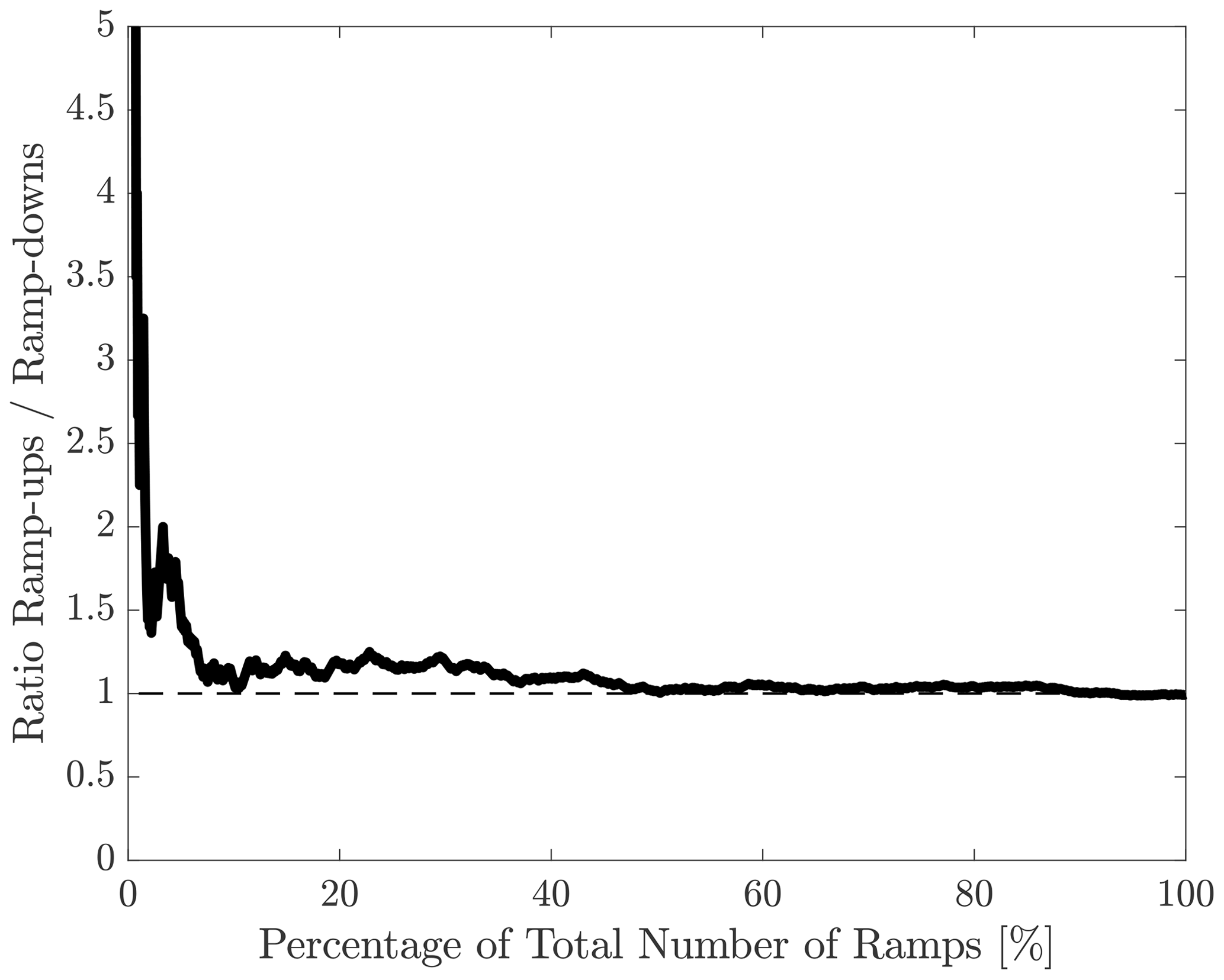
Amongst the 1183 ramps analysed, 590 (49.87 %) were ramp-ups. The equal proportion between ramp-ups and ramp-downs exhibited in the data set could be seen as a contradiction, with other studies (Freedman et al., 2008; Ferreira et al., 2012; Kamath, 2010; Jørgensen and Mohrlen, 2008) suggesting ramp-ups are more frequent as they often result from rapidly moving transient features causing a sharp increase in wind power followed by a gradual decrease (Freedman et al., 2008; Ferreira et al., 2012). However, the even ratio between ramp-ups and ramp-downs observed in this study is a direct consequence of the broad temporal coverage of ramps considered within the power generation time series. It is naturally expected that the proportion of ramp-ups vs. ramp-downs converges towards 1 as the proportion of investigated variability increases. This behaviour is depicted in Fig. 8 showing the ratio of ramp-ups / ramp-downs as a function of the number of strongest ramps considered in the data set. When considering larger power fluctuations (i.e. ramps associated with higher normalised ramp scores Rnorm), the ramp-up / ramp-down ratio increases as stronger ramps are more frequently ramp-ups. These findings are thus consistent with previous studies.
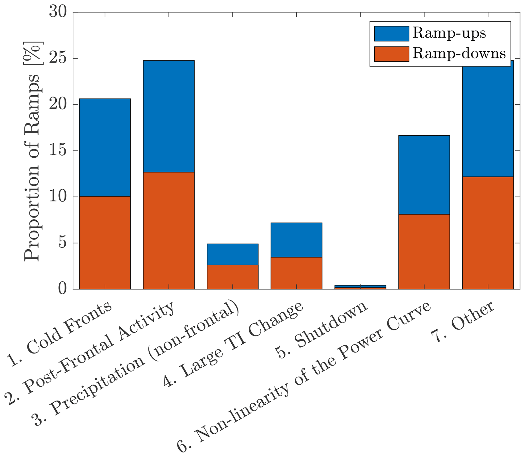
Figure 9Categorisation of intra-hourly wind power ramps between 1 October 2016 and 1 March 2019.
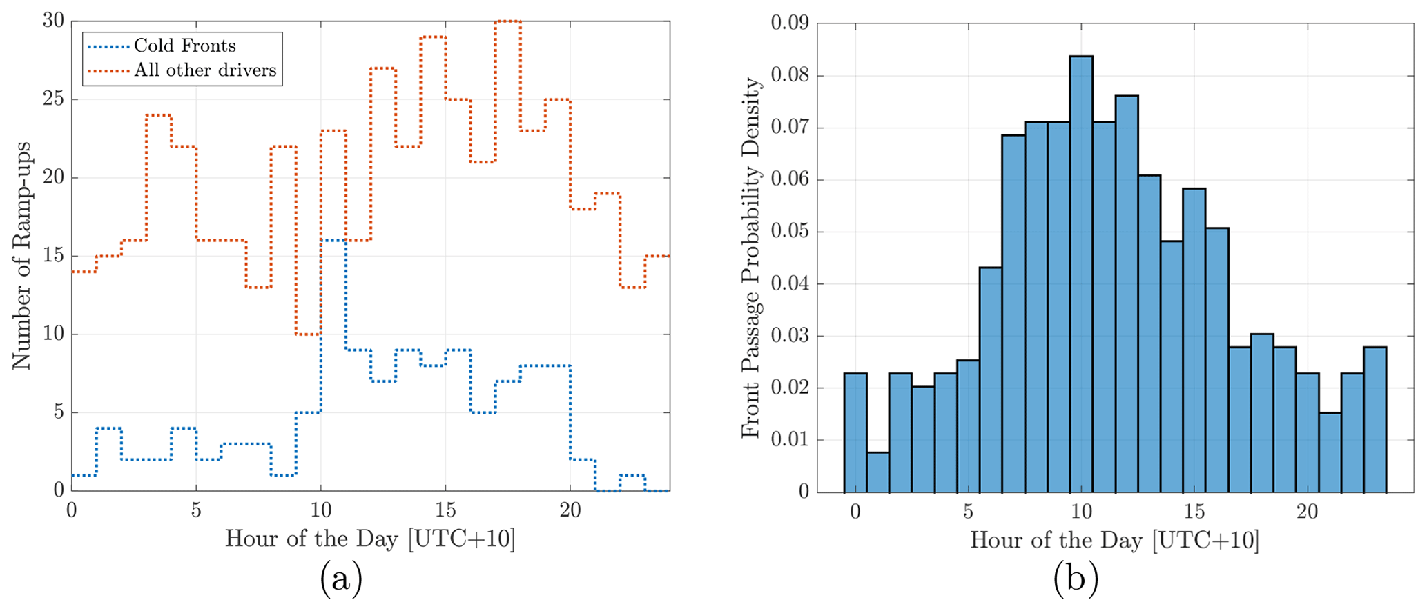
Figure 10(a) Hourly distribution of ramps associated with cold fronts vs. all other drivers and (b) hourly front distribution based on the adapted Melbourne Frontal Tracking Scheme between 1 October 2016 and 1 March 2019.
3.2 Ramp categorisation
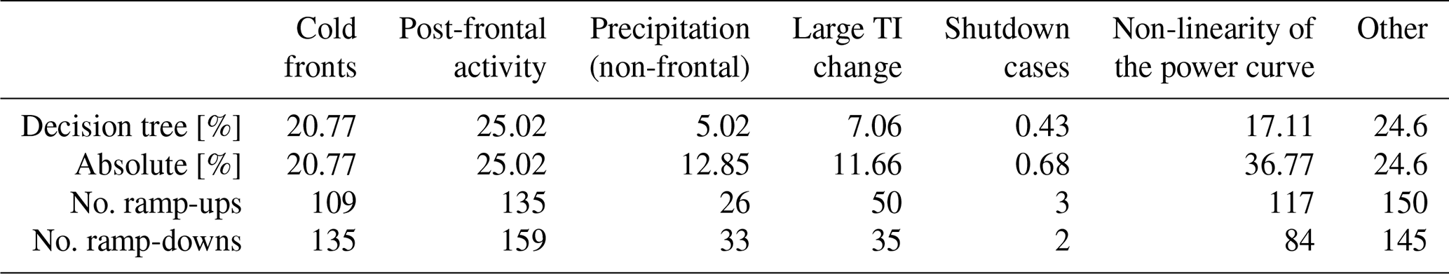
Figure 9 presents the distribution of ramps according to their underlying processes. The proportion of each driver category (following the decision tree in Fig. 5) and each criterion considered alone, together with the total number of ramps for each driver category, are provided in Table 1. Of the intra-hourly ramps at the wind farm site, 46 % are related to frontal activity, with cold fronts and post-frontal conditions accounting for 21 % and 25 % of the ramps, respectively. Precipitation and events associated with a large TI change account for 5 % and 7 % of the ramps, respectively. Times during which the wind farm production is externally restrained due to high winds are relatively rare, accounting for only 0.4 % of the ramps within the data set. Up to 17 % of the ramps sorted by the decision tree are associated with small variations in wind speed along the 5–10 m s−1 section of the power curve. When considered separately, the “non-linearity of the power curve” criterion was identified as a factor for approximately 37 % of the ramps (Table 1), demonstrating the importance of accurate wind predictions within this range. Overall, all drivers instigate both upward and downward ramps, as per the expected processes described in Sect. 2.5.
Figure 10a shows the diurnal distribution of cold-front ramp-ups against all other ramp-ups; the observed 10:00 peak in ramp-ups observed in Fig. 7a appears to be closely related to the timing of frontal passages. In fact, most 10:00 ramp-ups are associated with cold fronts (41 %). Likewise, a majority (42 %) of downward ramps observed at 15:00 UTC+10 are associated with post-frontal conditions (explained by the relaxation of wind speed after the passage of a front causing downward ramps). To investigate this further, we consider the hourly distribution of frontal passages during the assessment period based on the adaptation of the front identification algorithm of Simmonds et al. (2012) discussed above (Fig. 10b), where a clear 10:00 maximum frequency of incidence is observed. These findings are consistent with the findings of Berson et al. (1957), in which an early-afternoon maximum in the frontal passage was reported in the region.
A number of caveats need to be considered for the ramp classification scheme. First, off-site precipitation data were used to determine precipitation-related ramps. One needs to be careful with implementing such a method as localised showers with short spatial and temporal scales might lead to the misleading identification of rain events. After classification, 25 % of the ramps could not be directly attributed to one of the categories introduced above. While the proposed approach effectively portrays the prevalence of the most likely ramp drivers, we acknowledge the method cannot capture all possible events inducing ramps. For example, meteorological phenomena such as microbursts, gravity waves and low-level jets were not directly assessed, although they may implicitly appear in some of the categories. In addition, the ramp classification does not consider other mechanical processes such as wake effects and yaw misalignment (their contribution in explaining ramp events is expected to be marginal). Finally, the front detection algorithm is limited by the fact that it is based on a single point measurement. As discussed in Sect. 3.4, some ramps classified as “other” are in fact associated with the passage of fronts or troughs.
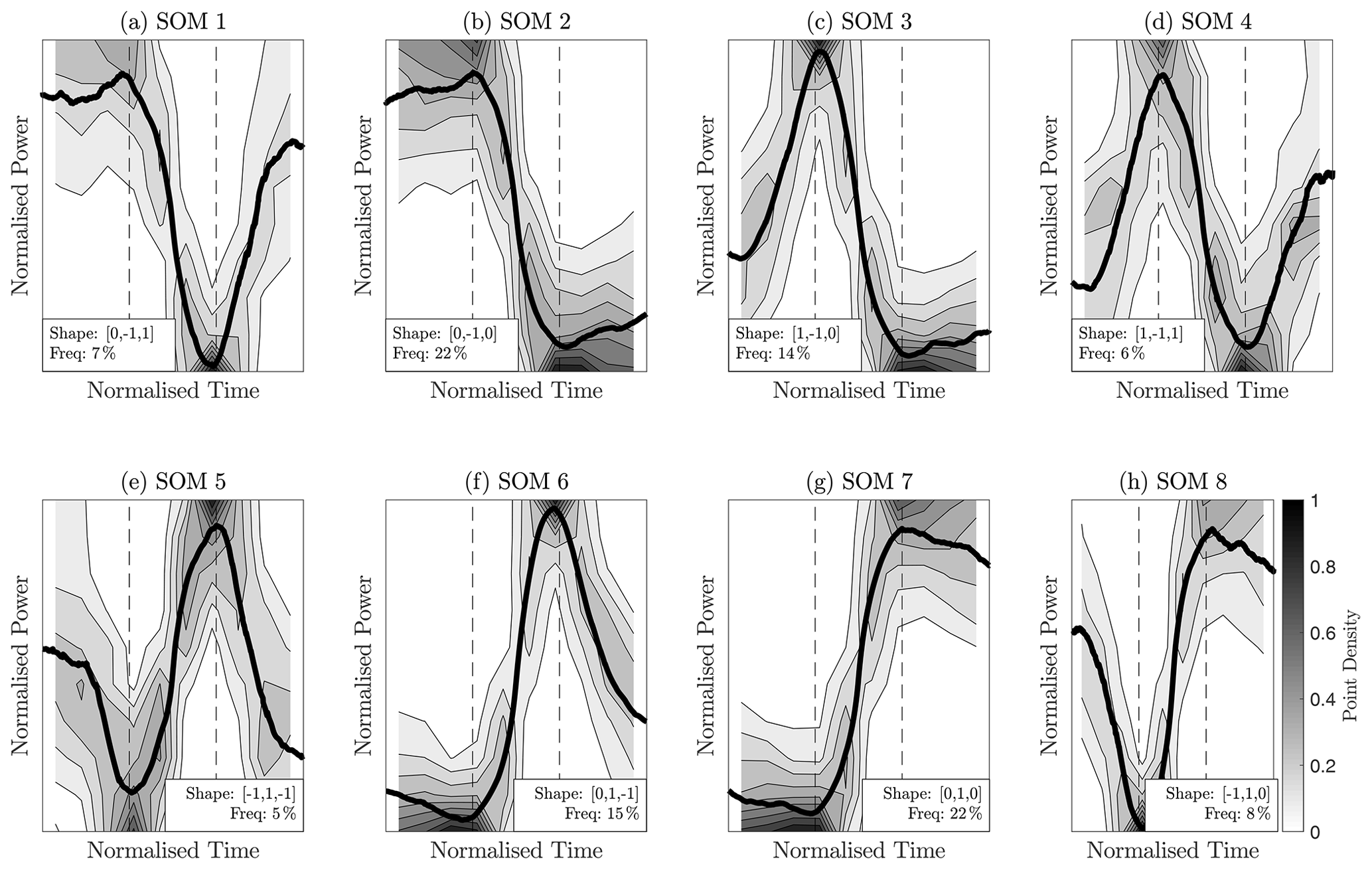
Figure 11Extended ramp shape classes resulting from SOM clustering. The thick black lines show the averaged extended ramp shape, and the grayscale contours display the point density for each SOM group. The dashed lines delineate periods equal to one rise time.
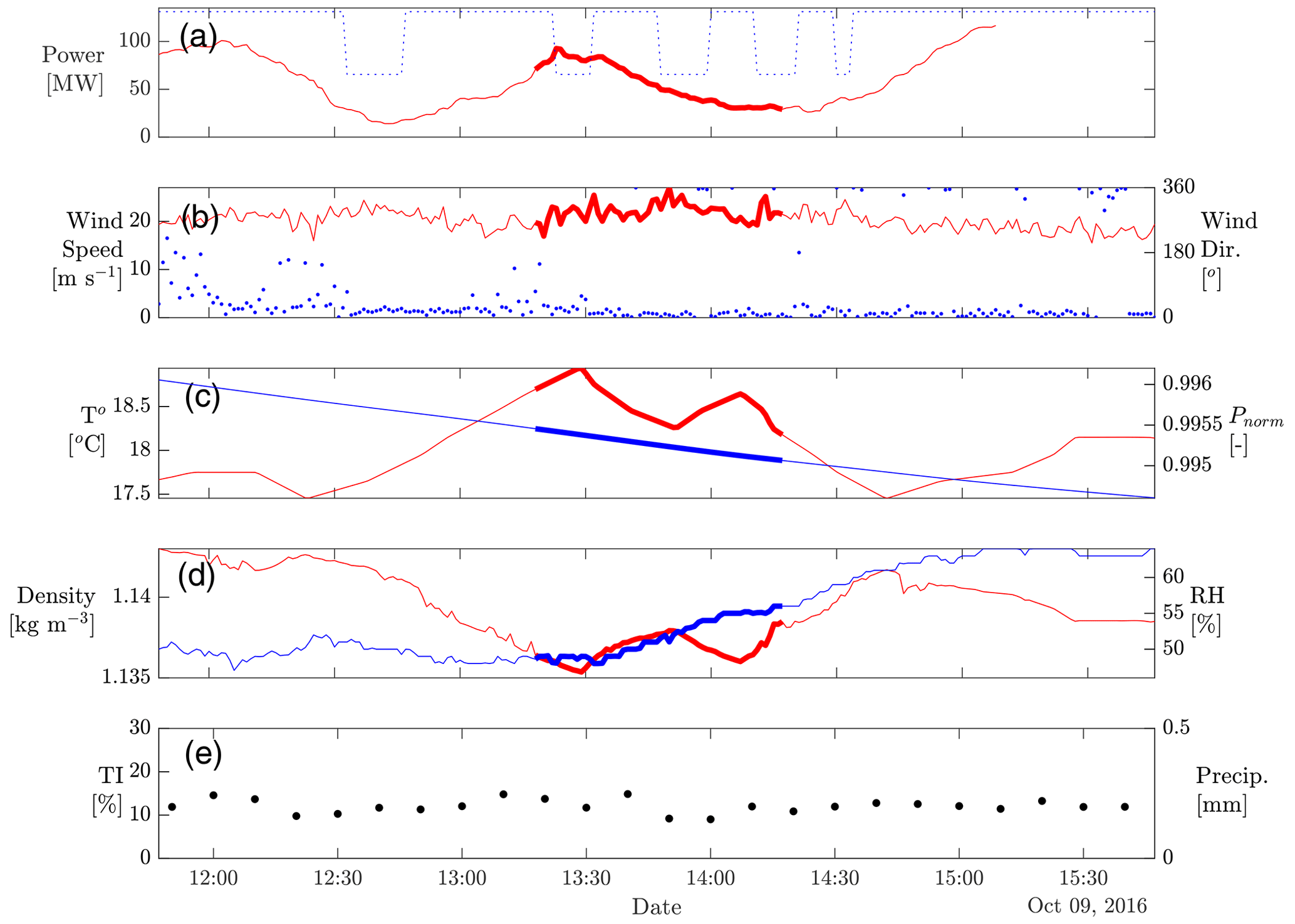
Figure 12Time series of environmental variables encompassing the ramp on 9 October 2016 at 13:47:00 (UTC+10). (a) Total wind farm power generation (red line) and mean wind power (mean wind speed from the two on-site meteorological towers converted to wind power based on the turbine's power curve and the number of turbines actively generating; dashed blue line), (b) mean wind speed (red line) and wind direction (blue dots), (c) temperature and 30 min normalised pressure (red and blue line, respectively), (d) air density and relative humidity (red and blue line, respectively), and (e) mean horizontal turbulence intensity over a 10 min window (black dots). Thickened red lines correspond to the extent of the ramp scale.

Figure 13(a) Time series of environmental variables encompassing the ramp on 7 December 2017 at 16:43:00 (UTC+10). (b) MSLP chart on 7 December 2017, 16:00:00 (UTC+10) (source: Australian Bureau of Meteorology). The blue bars in (a) indicate precipitation recorded at the weather station neighbouring the site (Sheoaks). The red cross in (b) indicates the approximate location of the site.
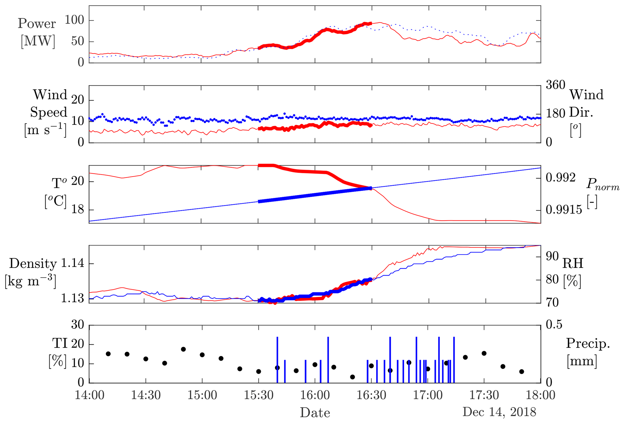
Figure 14Time series of environmental variables encompassing the ramp on 14 December 2018 at 16:00:00 (UTC+10). The blue bars indicate precipitation recorded at the weather station neighbouring the site (Sheoaks).
3.3 Extended ramp shape
Figure 11 displays the variety of power fluctuation behaviours obtained through self-organising maps with eight groups (SOM1–SOM8). For clarity, the thick black lines represent the mean extended ramp shape and the grayscale contours display the point density for each SOM group. The dashed lines delineate periods equal to one rise time. The trend of the fluctuations before, during and after the ramp is characterised by , in which x, y and z can exhibit three discrete values: 0 for a plateauing trend, −1 for a downward trend and 1 for an upward trend. The relative proportion of ramps within each group is also indicated in Fig. 11. The categories resulting from the SOMs correspond to the eight shape classes expected when assuming power generation can either level out or follow an inverse trend before and after the ramp.
While results from the SOMs indicate a great variability in extended ramp behaviour, specific shape classes exhibit different patterns. In particular, fluctuations commonly tend to plateau before and after the ramp, with such behaviour being observed for 44 % of the ramps (22 % for both and ). Peaking ramps, namely and , account for 15 % and 14 % of the data set, respectively. The representations of other SOM groups are all less than 10 %.
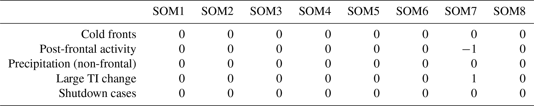
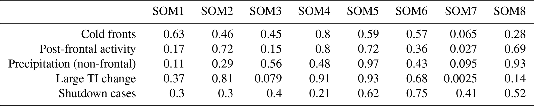
Bootstrapping tests failed to identify statistically significant interactions between extended ramp shapes and ramp drivers in most cases, with the exception of plateauing ramp-ups (SOM7; ). In particular, plateauing ramp-ups are found to be less frequent under post-frontal conditions. Post-frontal processes are indeed expected to exhibit continuously oscillating features rather than a steady increase between two power generation levels. On the other hand, ramps associated with a large change in TI are found to display proportionally more SOM7 compared to the other ramp drivers. Overall, these findings do not suggest there is a strong relationship between ramp drivers and ramp shape. Specific results from the bootstrap test and associated p values are provided in Tables A1 and A2 in Appendix A.
3.4 Case studies
In this section, we present several characteristic events with further details on the association between environmental conditions and wind farm generation. The case studies are for illustrative purposes and put into perspective the ramp driver classes introduced earlier.
-
Case Study 1, high winds during ramp on 9 October 2016. Strong winds were recorded throughout the day, with the maximum wind speed exceeding 28 m s−1. The automatic ramp categorisation scheme detected two ramp-downs at 12:26 and 13:47 UTC+10, directly followed by a ramp-up at 14:42 UTC+10. Environmental conditions centred on the ramp at 13:47 are provided in Fig. 12. It is evident from Fig. 12a that wind power largely exceeded generated power and its variations are not accompanied by analogous changes in generated power throughout the day. This is explained by the fact that groups of turbines periodically initiated a shutdown–restart procedure to prevent structural load or turbine damage. In addition, rapid changes in wind direction observed during the day have caused misalignment between the wind direction and the axis of the turbine rotor blades, hence diminishing the wind power generated.
-
Case Study 2, passage of a cold front on 7 December 2017. A typical example of a ramp associated with a cold front is presented in Fig. 13a, during which the power generation increased by 83 MW (63 % rated power) in 26 min. Figure 13a shows typical cold-front features such as a shift in wind from the northwest to the southwest quadrant together with decreasing temperature, increasing air density and precipitation. Analysis of the MSLP chart shortly before the ramp (Fig. 13b) agrees with the cold-front classification by the automatic ramp categorisation scheme.
-
Case Study 3, passage of a storm on 14 December 2018. Severe thunderstorm activity was recorded throughout the day, leading to flash flooding in the region (Press, 2018). Figure 14 shows a mid-afternoon increase in relative humidity coupled with a drop in temperature and precipitation, likely associated with the onset of convective activity. The increased wind speeds, likely associated with the thunderstorm downdraft, resulted in a 59 MW amplitude ramp-up centred at 16:00 UTC+10 (Fig. 14). The relaxation in wind speeds following the passage of the storm induced a downward ramp at 16:43 UTC+10, with an amplitude of 43 MW. The classification algorithm adequately categorised both ramps as non-frontal precipitation events.
-
Case Study 4, other – cold air outbreak with cellular convection on 25 September 2017. As discussed in Sect. 2.4, not all meteorological phenomena are captured through the ramp classification scheme. An example categorised as other took place at 14:34 UTC+10 on 25 September 2017; a day characterised by constant power generation fluctuations (Fig. 15a). Satellite imagery around the timing of the ramp (Fig. 15b) suggests the variability observed throughout the day is attributable to sustained cellular convection, which has been shown to drive wind speed fluctuations (Vincent et al., 2012). In particular, MSLP charts indicate a low-pressure system with an embedded front passing over the site at around 01:00 AEST on the same day, and as such, the ramp should be considered a particular case of post-frontal convection. While the automatic front identification scheme accurately detected the frontal passage, the ramp was not associated with post-frontal conditions because it occurred more than 12 h after the cold front.

Figure 15(a) Time series of environmental variables encompassing the ramp on 25 September 2017 at 14:34:00 (UTC+10). (b) Satellite imagery on 25 September 2017, 14:45:00 (UTC+10) (source: MODIS, 2020). The properties of the plots in (a) are analogous to Fig. 12. The red cross in (b) indicates the approximate location of the site.
Sudden wind power variations and associated underlying processes need to be accurately characterised to enhance ramp forecast accuracy and hence reduce grid instability. Although the influence of more common (i.e. less extreme) wind power ramps is evident, the current body of literature on ramp characterisation focuses mostly on the largest ramps owing to a lack of an automated classification methodology. This paper bridges this knowledge gap by assessing power variations with a temporal coverage exceeding 5 %. In this study, we introduced a robust method to characterise intra-hourly wind power ramps at the wind farm scale. We then explored the underlying causes of the identified ramps. Finally, we investigated the shape of the fluctuations surrounding ramps to improve ramp modelling.
The results are significant in three respects. First and foremost, we show how simple statistics can provide valuable insights into the complex mechanisms shaping ramp event dynamics. Second, although the behaviour of the power fluctuations before and after a ramp can vary greatly, some ramping behaviours are more frequent than others. For instance, power fluctuations tend to plateau before and after the ramp in 44 % of the cases. Such considerations need to be accounted for when modelling ramps. Third, the study showed that cold fronts and post-frontal activity accounted for most of the ramps investigated (46 %). Implications in terms of forecastability are significant. As passages of cold fronts are often predictable several days in advance using numerical weather prediction models, albeit with timing errors, these can be used to warn operators in the control room of days with high chances of ramp occurrence. Likewise, wind farm operators can expect more wind power variability within 12 h of the passage of a front (post-frontal conditions). Similarly, precipitation events can be challenging to predict accurately more than a couple of hours in advance, particularly where stochastic convective-scale processes are present.
The present research opens up new lines of inquiry into the existing relationships between frontal passages and wind power ramps. In particular, it would be helpful to explore further whether fronts always result in wind power ramps at the wind farm scale. The results presented here also indicate the potential for real-time, upstream ramp detection using remote sensing and in situ observations. Finally, we note that the accurate modelling and prediction of wind power ramps is also beneficial to other areas of research, such as aviation safety and building design.
In this paper, we use a bootstrapping approach to assess whether specific ramp drivers have characteristic ramp shapes. Bootstrapping is a common statistical test used to evaluate the sampling distribution of a variable based on random sampling. The population is sampled a number of times equal to the number of samples (there are 1183 ramps in the data set), according to weights given by the probability distribution assuming no relationships between the ramp shapes and drivers. This random sampling with replacement is repeated 1000 times. The observed ensemble frequencies falling outside of the 95 % confidence interval of their bootstrapped distributions indicate statistically significant differences. Results from the bootstrap test and associated p values are provided in Table A1 and A2, respectively.
Table A1Interactions between ramp driver and associated shape class – results from the bootstrap test in which −1 represents observations below the 95 % confidence interval lower bound from the bootstrapped distribution, 1 represents observations higher than the 95 % confidence interval upper bound and 0 denotes no statistically significant differences.
MSLP charts and satellite imagery data presented in this study can be accessed online at http://www.bom.gov.au/australia/charts/archive/ (BOM, 2020b) and https://modis-images.gsfc.nasa.gov/ (MODIS, 2020), respectively. Wind farm power generation data are confidential and therefore not publicly available. Environmental data presented in this study are available from the Bureau of Meteorology.
All authors contributed to the design and implementation of the research and the analysis of the results. MP wrote the manuscript with input from CV, GS and JM.
The authors declare that they have no conflicts of interest.
This study is partly funded by the Australian Renewable Energy Agency (ARENA) in the context of the Market Participant 5-Minute forecast (MP5F) initiative undertaken by the Australian Renewable Energy Agency (ARENA) and the Australian Energy Market Operator (AEMO). We would like to thank Meridian Energy Australia for providing the data presented in this study.
This research has been supported by the Australian Renewable Energy Agency (ARENA) (grant no. 2018/ARP16).
This paper was edited by Joachim Peinke and reviewed by Ásta Hannesdóttir and one anonymous referee.
Berson, F. A., Reid, D. G., and Troup, A. J.: The Summer Cool Change of South-Eastern Australia, Technical Paper 8, Commonwealth Scientific and Industrial Research Organization, Melbourne, Australia, 1957. a
Bianco, L., Djalalova, I. V., Wilczak, J. M., Cline, J., Calvert, S., Konopleva-Akish, E., Finley, C., and Freedman, J.: A Wind Energy Ramp Tool and Metric for Measuring the Skill of Numerical Weather Prediction Models, Weather Forecast., 31, 1137–1156, https://doi.org/10.1175/WAF-D-15-0144.1, 2016. a
Bitsa, E., Flocas, H., Kouroutzoglou, J., Hatzaki, M., Rudeva, I., and Simmonds, I.: Development of a Front Identification Scheme for Compiling a Cold Front Climatology of the Mediterranean, Climate, 7, 130, https://doi.org/10.3390/cli7110130, 2019. a
BOM: Bureau of Meteorology Sheoaks Weather Station, available at: http://www.bom.gov.au/places/vic/she-oaks/, last access: 10 September 2020a. a
BOM: Bureau of Meteorology MSLP Charts, http://www.bom.gov.au/australia/charts/archive/, last access: 2 December 2020b. a
Bradford, K. T., Carpenter, D. R. L., and Shaw, B. L.: Forecasting Southern Plains Wind Ramp Events Using the WRF Model at 3-Km, The 9th American Meteorological Society Anual Meeting, 17 January 2010, p. 10, Altanta, GA, 2010. a
Couto, A., Costa, P., Rodrigues, L., Lopes, V. V., and Estanqueiro, A.: Impact of Weather Regimes on the Wind Power Ramp Forecast in Portugal, IEEE T. Sustain. Energ., 6, 934–942, https://doi.org/10.1109/TSTE.2014.2334062, 2015. a
Cui, M., Ke, D., Sun, Y., Gan, D., Zhang, J., and Hodge, B.-M.: Wind Power Ramp Event Forecasting Using a Stochastic Scenario Generation Method, IEEE T. Sustain. Energ., 6, 422–433, https://doi.org/10.1109/TSTE.2014.2386870, 2015. a
Cutler, N.: Characterising the Uncertainty in Potential Large Rapid Changes in Wind Power Generation, Ph.D. thesis, University of New South Whales, Sydney, 2009. a
Cutler, N., Kay, M., Jacka, K., and Nielsen, T. S.: Detecting, Categorizing and Forecasting Large Ramps in Wind Farm Power Output Using Meteorological Observations and WPPT, Wind Energy, 10, 453–470, https://doi.org/10.1002/we.235, 2007. a, b
Dee, D. P., Uppala, S. M., Simmons, A. J., Berrisford, P., Poli, P., Kobayashi, S., Andrae, U., Balmaseda, M. A., Balsamo, G., Bauer, P., Bechtold, P., Beljaars, A. C. M., van de Berg, L., Bidlot, J., Bormann, N., Delsol, C., Dragani, R., Fuentes, M., Geer, A. J., Haimberger, L., Healy, S. B., Hersbach, H., Hólm, E. V., Isaksen, L., Kållberg, P., Köhler, M., Matricardi, M., McNally, A. P., Monge-Sanz, B. M., Morcrette, J.-J., Park, B.-K., Peubey, C., de Rosnay, P., Tavolato, C., Thépaut, J.-N., and Vitart, F.: The ERA-Interim Reanalysis: Configuration and Performance of the Data Assimilation System, Q. J. Roy. Meteor. Soc., 137, 553–597, https://doi.org/10.1002/qj.828, 2011. a
Deppe, A. J., Gallus, W. A., and Takle, E. S.: A WRF Ensemble for Improved Wind Speed Forecasts at Turbine Height, Weather Forecast., 28, 212–228, https://doi.org/10.1175/WAF-D-11-00112.1, 2012. a, b
Efron, B.: Bootstrap Methods: Another Look at the Jackknife, Ann. Stat., 7, 1–26, https://doi.org/10.1214/aos/1176344552, 1979. a
EIA, U. E. I. A.: Annual Energy Outlook 2019 with Projections to 2050, Tech. rep., U.S Department of Energy, Washington, USA, 2019. a
Ferreira, C., Gama, J., Moreira-Matias, L., Botterud, A., and Wang, J.: A Survey on Wind Power Ramp Forecasting, Tech. Rep. ANL/DIS-10-13, Argonne National Laboratory, Illinois, USA, 2010. a
Ferreira, C. A., Gama, J., Santos Costa, V., Miranda, V., and Botterud, A.: Predicting Ramp Events with a Stream-Based HMM Framework, in: Discovery Science, edited by: Ganascia, J.-G., Lenca, P., and Petit, J.-M., Lecture Notes in Computer Science, 224–238, Springer Berlin Heidelberg, Berlin, Germany, 2012. a, b, c
Fournier, M. B. and Haerter, J. O.: Tracking the Gust Fronts of Convective Cold Pools, J. Geophys. Res.-Atmos., 124, 11103–11117, https://doi.org/10.1029/2019JD030980, 2019. a
Freedman, J., Markus, M., and Penc, R.: Analysis of West Texas Wind Plant Ramp-up and Ramp-down Events, Tech. rep., AWS Truewind, Texas, USA, 2008. a, b, c
Gallego, C., Costa, A., Cuerva, Á., Landberg, L., Greaves, B., and Collins, J.: A Wavelet-Based Approach for Large Wind Power Ramp Characterisation, Wind Energy, 16, 257–278, https://doi.org/10.1002/we.550, 2013. a, b, c, d, e, f
Gallego, C., Cuerva, Á., and Costa, A.: Detecting and Characterising Ramp Events in Wind Power Time Series, J. Phys. Conf. Ser., 555, 012040, https://doi.org/10.1088/1742-6596/555/1/012040, 2014. a, b
Gallego, C., Cuerva-Tejero, A., and Lopez-Garcia, O.: A Review on the Recent History of Wind Power Ramp Forecasting, Renewable and Sustainable Energy Reviews, 52, 1148–1157, https://doi.org/10.1016/j.rser.2015.07.154, 2015a. a, b, c
Gallego, C., García-Bustamante, E., Cuerva, Á., and Navarro, J.: Identifying Wind Power Ramp Causes from Multivariate Datasets: A Methodological Proposal and Its Application to Reanalysis Data, IET Renew. Power Gen., 9, 867–875, https://doi.org/10.1049/iet-rpg.2014.0457, 2015b. a
Greaves, B., Collins, J., Parkes, J., and Tindal, A.: Temporal Forecast Uncertainty for Ramp Events, Wind Engineering, 33, 309–320, https://doi.org/10.1260/030952409789685681, 2009. a
GWEC: Global Wind Report 2018, Annual Market Update, Tech. rep., GWEC, Brussels, Belgium, 2019. a
Hannesdóttir, Á. and Kelly, M.: Detection and Characterization of Extreme Wind Speed Ramps, Wind Energy Science, 4, 385–396, https://doi.org/10.5194/wes-4-385-2019, 2019. a, b, c
IEC: Wind Turbines – Power Performance Measurements of Electricity Producing Wind Turbines, International Standard IEC 61400-12-1:2005(E), International Electrotechnical Commission, Geneva, Switzerland, 2005. a
Jørgensen, J. U. and Mohrlen, C.: AESO Wind Power Forecasting Pilot Project, Tech. rep., WEPROG, Ebberup, Denmark, 2008. a, b, c
Kamath, C.: Understanding Wind Ramp Events through Analysis of Historical Data, IEEE PES T&D 2010, 1–6, IEEE, New Orleans, LA, USA, https://doi.org/10.1109/TDC.2010.5484508, 2010. a, b
Kariniotakis, G.: Renewable Energy Forecasting: From Models to Applications, Woodhead Publishing, Cambridge, UK, 2017. a
Kohonen, T.: Self-Organized Formation of Topologically Correct Feature Maps, Biol. Cybern., 43, 59–69, https://doi.org/10.1007/BF00337288, 1982. a
Lacerda, M., Couto, A., and Estanqueiro, A.: Wind Power Ramps Driven by Windstorms and Cyclones, Energies, 10, 1475, https://doi.org/10.3390/en10101475, 2017. a
Lange, M., Focken, U., and Lenz, A.: Ramp Event Forecasting – Practical Experiences in the USA and Australia, 9th International Workshop on Large-Scale Integration of Wind Power into Power Systems as Well as on Transmission Networks for Offshore Wind Power Plants, 89–92, 18 October 2010, Québec, Canada, 2010. a
Magerman, B.: Short-Term Wind Power Forecasts Using Doppler Lidar, Ph.D. thesis, Arizona State University, Tempe, USA, 2014. a
Martínez-Arellano, G., Nolle, L., Cant, R., Lotfi, A., and Windmill, C.: Characterisation of Large Changes in Wind Power for the Day-Ahead Market Using a Fuzzy Logic Approach, KI – Künstliche Intelligenz, 28, 239–253, https://doi.org/10.1007/s13218-014-0322-3, 2014. a
Mishra, S., Leinakse, M., and Palu, I.: Wind Power Variation Identification Using Ramping Behavior Analysis, Enrgy. Proced., 141, 565–571, https://doi.org/10.1016/j.egypro.2017.11.075, 2017. a, b, c
MODIS: Atmosphere (NASA): MODIS L1B Granule Images, available at: https://modis-images.gsfc.nasa.gov/IMAGES/, last access: 9 September 2020. a, b
Percival, D. B. and Walden, A. T.: Wavelet Methods for Time Series Analysis by Donald B. Percival, https://doi.org/10.1017/CBO9780511841040, 2000. a, b
Potter, B. E. and Hernandez, J. R.: Downdraft Outflows: Climatological Potential to Influence Fire Behaviour, Int. J. Wildland Fire, 26, 685, https://doi.org/10.1071/WF17035, 2017. a, b
Press, A. A.: Victoria Hit by Destructive Thunderstorms as Bureau Warns NSW Is Next, The Guardian, available at: https://www.theguardian.com/weather/2018/dec/15/victoria-braces-for-more-flooding-and-thunderstorms (last access: 28 April 2020, Sydney, Australia, 2018. a
Sherry, M. and Rival, D.: Meteorological Phenomena Associated with Wind-Power Ramps Downwind of Mountainous Terrain, J. Renew. Sustain, Ener., 7, 033101, https://doi.org/10.1063/1.4919021, 2015. a, b, c
Simmonds, I., Keay, K., and Tristram Bye, J. A.: Identification and Climatology of Southern Hemisphere Mobile Fronts in a Modern Reanalysis, J. Climate, 25, 1945–1962, https://doi.org/10.1175/JCLI-D-11-00100.1, 2012. a, b
Steiner, A., Köhler, C., Metzinger, I., Braun, A., Zirkelbach, M., Ernst, D., Tran, P., and Ritter, B.: Critical Weather Situations for Renewable Energies – Part A: Cyclone Detection for Wind Power, Renew. Energ., 101, 41–50, https://doi.org/10.1016/j.renene.2016.08.013, 2017. a
Tayal, D.: Achieving High Renewable Energy Penetration in Western Australia Using Data Digitisation and Machine Learning, Renewable and Sustainable Energy Reviews, 80, 1537–1543, https://doi.org/10.1016/j.rser.2017.07.040, 2017. a
Treinish, L. A. and Treinish, L. A.: Precision Wind Power Forecasting via Coupling of Turbulent-Scale Atmospheric Modelling with Machine Learning Methods, 93rd American Meteorological Society Annual Meeting, AMS, 9 January 2013, Austin, USA, 2013. a
Trombe, P.-J., Pinson, P., and Madsen, H.: A General Probabilistic Forecasting Framework for Offshore Wind Power Fluctuations, Energies, 5, 621–657, https://doi.org/10.3390/en5030621, 2012. a
UNFCCC: Adoption of the Paris Agreement, Tech. rep., UNFCCC, Paris, 2015. a
van Kooten, G. C.: Wind Power: The Economic Impact of Intermittency, Letters in Spatial and Resource Sciences, 3, 1–17, https://doi.org/10.1007/s12076-009-0031-y, 2010. a
Vincent, C. L., Hahmann, A. N., and Kelly, M. C.: Idealized Mesoscale Model Simulations of Open Cellular Convection Over the Sea, Bound.-Lay. Meteorol., 142, 103–121, https://doi.org/10.1007/s10546-011-9664-7, 2012. a
Worsnop, R. P., Scheuerer, M., Hamill, T. M., and Lundquist, J. K.: Generating Wind Power Scenarios for Probabilistic Ramp Event Prediction Using Multivariate Statistical Post-Processing, Wind Energy Science, 3, 371–393, https://doi.org/10.5194/wes-3-371-2018, 2018. a
Wurth, I., Ellinghaus, S., Wigger, M., Niemeier, M. J., Clifton, A., and Cheng, P. W.: Forecasting Wind Ramps: Can Long-Range Lidar Increase Accuracy?, J. Phys. Conf. Ser., 1102, 012013, https://doi.org/10.1088/1742-6596/1102/1/012013, 2018. a
Wurth, I., Valldecabres, L., Simon, E., Möhrlen, C., Uzunoğlu, B., Gilbert, C., Giebel, G., Schlipf, D., and Kaifel, A.: Minute-Scale Forecasting of Wind Power–Results from the Collaborative Workshop of IEA Wind Task 32 and 36, Energies, 12, 712, https://doi.org/10.3390/en12040712, 2019. a
Zack, J., Mendes, J., Bessa, R., Keko, H., Miranda, V., Ferreira, C., Gama, J., Botterud, A., Zhou, Z., and Wang, J.: Development and Testing of Improved Statistical Wind Power Forecasting Methods, Tech. Rep. ANL/DIS-11-7, Argonne National Laboratory, Illinois, USA, 2011. a
Zhang, J., Florita, A., Hodge, B.-M., and Freedman, J.: Ramp Forecasting Performance From Improved Short-Term Wind Power Forecasting, in: Volume 2A: 40th Design Automation Conference, p. V02AT03A022, ASME, Buffalo, New York, USA, https://doi.org/10.1115/DETC2014-34775, 2014. a
Zhang, J., Cui, M., Hodge, B.-M., Florita, A., and Freedman, J.: Ramp Forecasting Performance from Improved Short-Term Wind Power Forecasting over Multiple Spatial and Temporal Scales, Energy, 122, 528–541, https://doi.org/10.1016/j.energy.2017.01.104, 2017. a, b