the Creative Commons Attribution 4.0 License.
the Creative Commons Attribution 4.0 License.
 | 30 Nov 2021
On turbulence models and lidar measurements for wind turbine control
Wai Hou Lio
Eric Simley
To provide comprehensive information that will assist in making decisions regarding the adoption of lidar-assisted control (LAC) in wind turbine design, this paper investigates the impact of different turbulence models on the coherence between the rotor-effective wind speed and lidar measurement. First, the differences between the Kaimal and Mann models are discussed, including the power spectrum and spatial coherence. Next, two types of lidar systems are examined to analyze the lidar measurement coherence based on commercially available lidar scan patterns. Finally, numerical simulations have been performed to compare the lidar measurement coherence for different rotor sizes. This work confirms the association between the measurement coherence and the turbulence model. The results indicate that the lidar measurement coherence with the Mann turbulence model is lower than that with the Kaimal turbulence model. In other words, the potential value creation of LAC based on simulations during the wind turbine design phase, evaluated using the Kaimal turbulence model, will be diminished if the Mann turbulence model is used instead. In particular, the difference in coherence is more significant for larger rotors. As a result, this paper suggests that the impacts of different turbulence models should be considered uncertainties while evaluating the benefits of LAC.
- Article
(2579 KB) - Full-text XML
- BibTeX
- EndNote


Turbine-mounted lidar sensors provide preview information about the inflow wind to be used for improving wind turbine control, which is referred to as wind-turbine-integrated lidar-assisted control (LAC). LAC is a promising technology for reducing wind turbine loads and the levelized cost of energy (LCOE) (Scholbrock et al., 2016; Simley et al., 2020; Schlipf et al., 2018). The potential benefits have been demonstrated in several works by simulation (Schlipf et al., 2010; Bossanyi, 2013; Schlipf et al., 2013b; Bossanyi et al., 2014) as well as in field experiments (Kumar et al., 2015; Fleming et al., 2014; Schlipf et al., 2014).
The topic of the optimal lidar scan pattern for wind energy applications is critical for the widespread deployment of LAC. Both practical considerations for overcoming the obstacles of LAC application and for optimizing lidar scan patterns were discussed at the International Energy Agency (IEA) Wind Task 32 workshop (Simley et al., 2018). Three commonly used simulated measurement quality metrics for LAC application are defined in Simley et al. (2018): magnitude-squared coherence between the true rotor-effective wind speed (REWS) and the lidar-based estimate, mean square error (MSE) between the true REWS and the lidar-based estimate, and MSE between the generator speed and the rated generate speed. The REWS is commonly used to indicate the rotor-averaged wind condition. The correlation between the REWS measured by the lidar and experienced by the rotor has been discussed in Haizmann et al. (2015), Simley et al. (2012) and Schlipf et al. (2013a), in which the magnitude-squared coherence is suggested as a key metric to quantify the measurement quality. A fundamental component of simulation-based lidar measurement coherence is the theoretical spatial coherence of the turbulence: (a) the lateral–vertical spatial coherence is defined in the International Electrotechnical Commission (IEC) design standard (IEC, 2019); (b) wind evolution models (Bossanyi, 2013; Simley and Pao, 2015) are defined in terms of longitudinal spatial coherence. Note that the actual coherence in the field could be different from the theoretical coherence; thus experimental validation by field testing is important as well.
According to current wind turbine design requirements in the IEC standard (IEC, 2019), for the standard wind turbine classes the turbulence model must contain the following elements: the turbulence standard deviation, the longitudinal turbulence scale parameters and a recognized model for the coherence. The standards recommend the use of either the Kaimal turbulence model, together with a standard exponential lateral–vertical coherence model, or the Mann turbulence model to represent the random wind velocity field. Although extensive research has been carried out on evaluating lidar measurement coherence, there is a clear knowledge gap regarding the impact of different turbulence models on the lidar measurement coherence. The wind field model used in most of the above-mentioned studies consists of the Kaimal turbulence spectrum and the lateral–vertical spatial coherence model defined in the IEC standard (IEC, 2019). The impact of different turbulence models on the dynamic response of an offshore wind turbine has been evaluated by Nybø et al. (2020); the results showed that as the rotor size becomes larger, the variation of the wind in time and space also becomes increasingly important. There is a need to evaluate the load reduction potential of LAC using different turbulence models, which is critical for determining the value creation of LAC during the wind turbine design phase. Held and Mann (2019) extended the previous works by Haizmann et al. (2015), Simley et al. (2012) and Schlipf et al. (2013a) to analyze lidar measurement coherence with both the Mann turbulence model and Kaimal turbulence model. The theoretical-coherence results were compared to field data from a nacelle lidar mounted on a Vestas V52 wind turbine. The results showed that the experimental data fit better to the coherence predicted by the Mann turbulence model, and the prediction based on the Kaimal turbulence model underestimates the coherence. However, the coherence analysis focused solely on a turbine with a small rotor diameter of 52 m; the impact of different rotor sizes and lidar scan patterns on coherence have not been investigated by Held and Mann (2019).
With the advent of larger rotor sizes and more flexible wind turbines, evaluating the value creation of LAC is becoming increasingly important. The analysis in this work is based on the framework proposed by Simley et al. (2018) and Held and Mann (2019). The specific objective of this study is to investigate the impact of different turbulence models recommended by the IEC standards on the lidar measurement coherence, especially for large rotor sizes (i.e., the Technical University of Denmark – DTU – 10 MW reference turbine with a rotor diameter of 178 m; Bak et al., 2013), whereby the analysis can shed light on how to reasonably evaluate LAC benefits during the wind turbine design phase. First the differences between the Kaimal and Mann models are discussed. Then two types of commercial continuous-wave (CW) lidar systems are examined to analyze the lidar measurement coherence, including a 4-beam lidar and 50-beam circular scan lidar. The lidar measurement model has been created based on work by Simley et al. (2011), and numerical simulations have been performed to compare the lidar measurement coherence.
The remainder of this paper is organized as follows: Sect. 2 briefly describes the different turbulence models and compares the power spectra. The lidar measurement model is established in Sect. 3. In Sect. 4, numerical simulations for different lidar scan patterns and rotor sizes are performed. Conclusions and suggestions for future work are summarized in Sect. 5.
Two different turbulence models are commonly used to evaluate the design loads in the IEC standard (IEC, 2019): the Kaimal spectrum with the exponential lateral–vertical coherence model (Kaimal model) and the Mann turbulence model (Mann model). The turbulence models use similar power spectra, and the major difference is the spatial distribution of the wind velocities.
2.1 Kaimal model
The advantage of the Kaimal model is that the one-dimensional spectra are expressed as simple analytic expressions. The wind disturbance is described as turbulent velocity fluctuations and is assumed to be a stationary and random vector field with zero-mean Gaussian statistics. The power spectral densities (PSDs) of each wind component are given in a non-dimensional form:
where f is the frequency in hertz, while the subscript k denotes the index of the velocity component in the longitudinal u, lateral v and upward w direction, respectively. The single-sided velocity component spectrum is denoted as Sk, while σk and Lk represent the standard deviation and integral length scale parameters of the velocity component, respectively. The wind speed at hub height is denoted as Vhub.
For the longitudinal velocity component u, σu is the representative value of the turbulence standard deviation, and Lu is defined as Lu=8.1Λu. For a modern wind turbine, the hub height is typically above z≥60 m, and the longitudinal length scale parameter is Λu=42 m.
The cross-power spectral density (CPSD) between the wind at the two spatially separated points of ui, uj can be determined from the definition of spatial co-coherence γi,j:
where and are the PSDs of the wind speed at two different locations, i and j. The symbol ℜ denotes the real part of a complex number. Please note that the coherence can be split into a real part and an imaginary part, which are referred to as co-coherence and quad-coherence (Nybø et al., 2020). The coherence expressed in Eq. (2) is in the real part form.
According to the IEC standard (IEC, 2019), the following exponential coherence model can be used in conjunction with the Kaimal PSD:
where r is the magnitude of the distance between the two points projected onto a plane normal to the averaged wind direction and Lc=Lu is the coherence scale parameter. The definition in Eq. (3) ignores the quad-coherence; thus the wind velocity fluctuations are assumed to be in phase. This assumption may be reasonable for small rotor sizes but can be questioned for larger rotor sizes (Eliassen and Obhrai, 2016).
2.2 Mann model
The Mann turbulence model (Mann, 1994) is a spectral tensor model based on von Kármán's model, which combines rapid distortion theory (RDT) with considerations about eddy lifetimes. The RDT in the Mann model gives an equation for the evolution or the “stretching” of the spectral tensor, and the tensor will be more and more “anisotropic” with time. The RDT will finally influence the lateral–vertical coherence in the rotor plane.
The three-dimensional fluctuations around the mean wind speed u(x) can be represented by the vector field
where is the turbulent velocity field and U(x) is the mean wind field.
Because of homogeneity, the covariance tensor is a function of the separation vector r between two points and is defined as follows:
where 〈 〉 denotes ensemble averaging.
All second-order statistics of turbulence, such as variances and cross spectra, can be derived from the covariance tensor. The spectral tensor is given by
where , is the non-dimensional spatial wavenumber for the three component directions and is the mean wind speed. The resulting spectral tensor components can be found in Annex C of the IEC standard (IEC, 2019).
For three-dimensional turbulent velocity vector u(x), the velocity components are determined from a decomposition of the spectral tensor and an approximation by discrete Fourier transform, following the procedure detailed in Mann (1998). Compared to the Kaimal spectrum and exponential coherence model, the advantage of using the Mann model to analyze lidar measurements is that it provides a three-dimensional spectral tensor. The Mann model includes correlation between the components (u, v, w), whereas the Kaimal model has no correlation between different wind components.
The Mann model is based on three adjustable parameters: (the Kolmogorov constant multiplied with the rate of the viscous dissipation of specific turbulent kinetic energy raised to the power of two-thirds), the length scale l and the non-dimensional parameter Γ related to the lifetime of the eddies.
The co-coherence γij for spatial separations (grid points i and j) normal to the longitudinal direction is defined as
where Δy is the lateral separation distance and Δz is the vertical separation distance. For the denominator in Eq. (7), when the two indices i=j, and the wavenumber auto-spectrum Ψii(k1) and Ψjj(k1) are expressed as
where the subscript .
2.3 Evaluation using different turbulence generators
The theoretical turbulence models are quite complicated, especially for the Mann model, although the application of the Mann model only requires three parameters (, l and Γ). Therefore, numerical simulations have been performed to compare the different turbulence models in this work.
2.3.1 Coordinate system
The coordinate system of the wind box as well as the lidar scan patterns is shown in Fig. 1. The size of the wind box should cover the entire rotor disk. The directions of the wind components (u, v, w) are aligned with the directions of the coordinate system axes (x, y, z). The lidar scan pattern will be elaborated in Sect. 3.2.
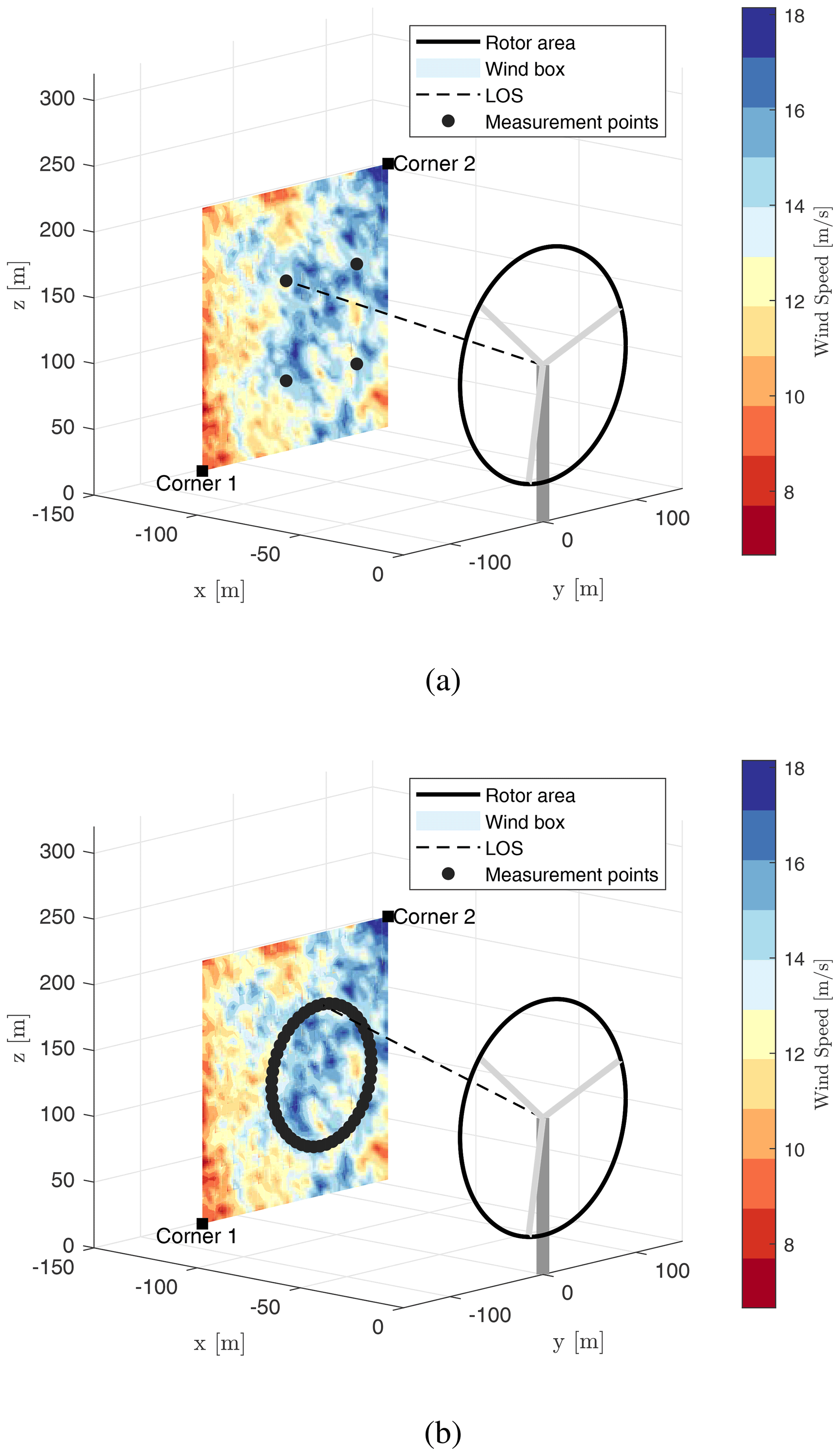
Figure 1Coordinate system of wind box and lidar scan patterns. The wind box is shown using the color map. Two corners are marked as black squares (corner 1 and corner 2). Two commercial CW lidar scan patterns are shown: (a) 4-beam CW lidar and (b) 50-beam circular scan CW lidar. The dashed line represents the line-of-sight direction.
2.3.2 Turbulence generator
To generate the wind boxes for further analysis, two different turbulence simulators are used. The Kaimal model can be generated using the turbulence simulator TurbSim (Jonkman and Buhl, 2006), while the Mann model is generated by HAWC2 (Horizontal Axis Wind turbine simulation Code 2nd generation; Hansen et al., 2018).
All numerical simulations are performed for a wind field with mean wind speed m s−1 and turbulence intensity given by the IEC Class A normal turbulence model (NTM). The parameters of the three-dimensional wind box are listed in Table 1. The grid size in the vertical and lateral directions is defined by the size of the wind box Lgrid and number of grid points Ngrids. Assuming Taylor's hypothesis of frozen turbulence, the grid size along the mean wind direction is defined as , where is the mean wind speed, T is the total time and Nx is the number of longitudinal grid points.
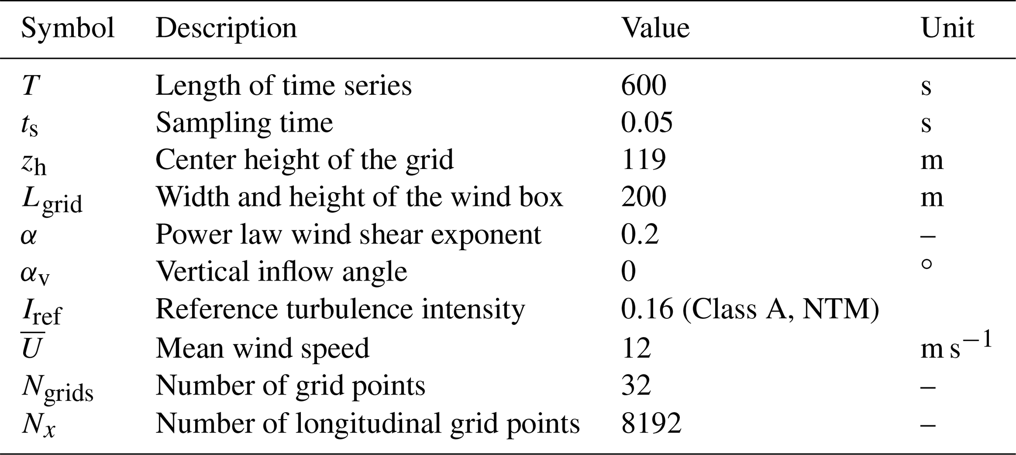
Since the Mann turbulence fields are normally rescaled to the specified turbulence intensity inside HAWC2, the parameter is chosen to be 1 and the shear parameter Γ should be approximately 3.9 for neutral conditions. The length scale l is recommended to be l=0.7Λu for normal conditions.
The method used in TurbSim is the Veers approach (Veers, 1988), wherein the PSDs in Eq. (1) and coherence function in Eq. (3) are used to correlate the Fourier components of different points in the y–z plane. Then the inverse fast Fourier transform (IFFT) is applied to obtain the correlated time series at each grid point. Although in the IEC standard the coherence function is only applied to the u component, the Veers approach is extended to apply the coherence to the components (v, w) in this work as well. It is assumed that the spatial coherence formula presented in Eq. (3) applies to all wind components (u, v, w), and the length scales for the different components are the same as defined for the PSDs. Otherwise, without the correlation of the v and w components the coherence between the REWS and its estimated value based on lidar measurements could be unrealistically high because the contribution of the v and w components could be close to zero after spatial averaging along the lidar beams (see Sect. 3.2). In contrast, the Mann model creates a turbulence field that is fully correlated in the directions of x, y and z.
2.3.3 Turbulence spectrum comparison
The differences between the Mann and Kaimal models are discussed in this section.
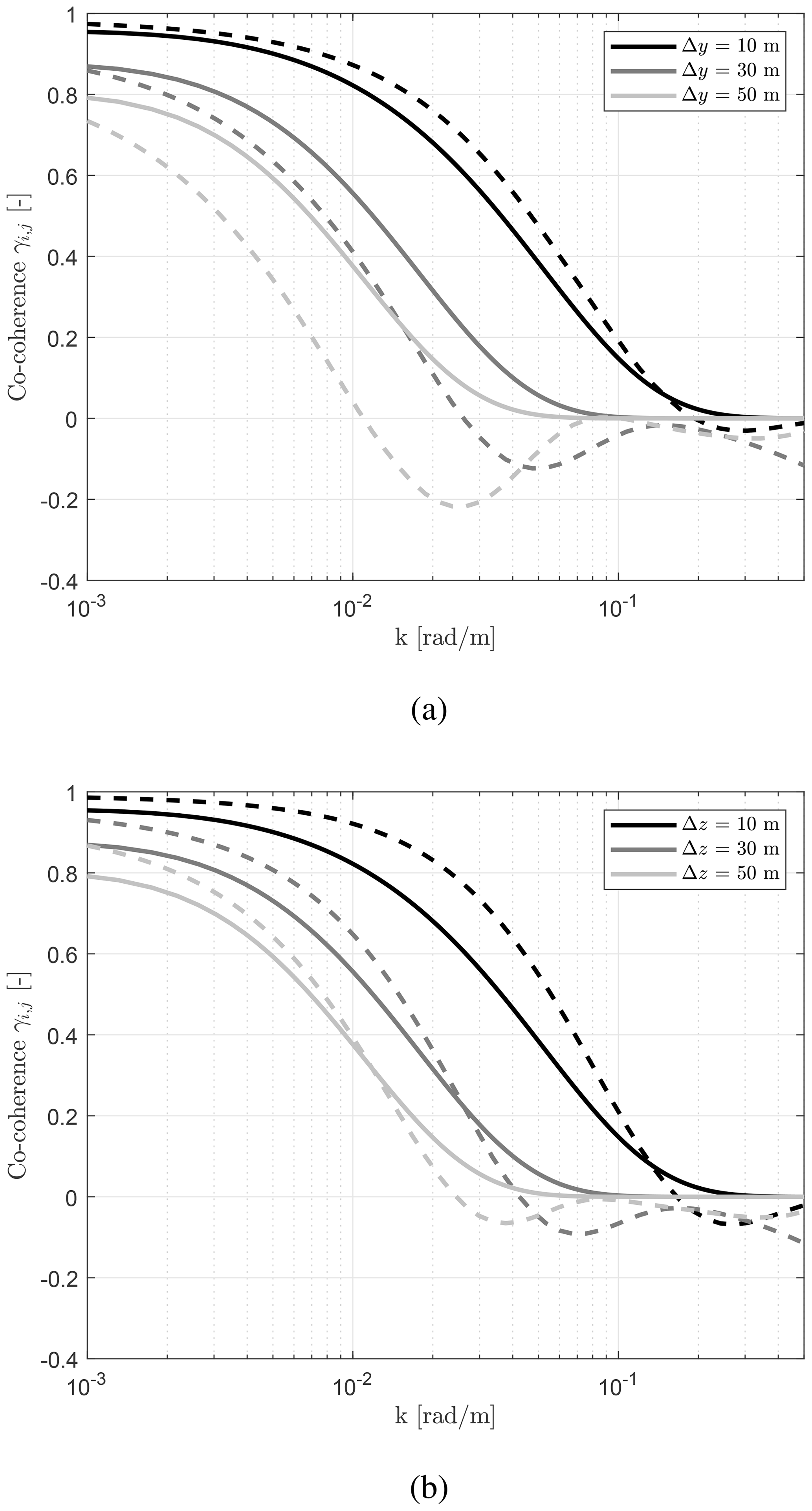
Figure 2Co-coherence at different separation distances. Δy and Δz represent the lateral and vertical separation distances, respectively. (a) Lateral co-coherence: Δz=0 m. (b) Vertical co-coherence: Δy=0 m. Dashed lines denote the Mann model, and solid lines denote the Kaimal model.
Figure 2 shows the theoretical co-coherence γi,j at different separation distances, in which the lateral separation distance Δy and vertical separation distance Δz are selected to be 10, 30 and 50 m. Some interesting findings are the following:
-
A clear trend can be seen in Fig. 2a, wherein the lateral co-coherence reduces as the lateral separation distance increases. With the small separation distance of 10 m, the coherence with the Mann model is higher than with the Kaimal model. Conversely, with increasing separation distance, the co-coherence with the Mann model falls sharply compared with the co-coherence with the Kaimal model; the co-coherence with the Mann model is far below the co-coherence with the Kaimal model for Δy=50 m.
-
For vertical separations in Fig. 2b, the co-coherence with the Mann model is always higher than that with the Kaimal model for low wavenumbers. Unlike the lateral co-coherence, the vertical co-coherence does not drastically decrease with increasing separation distance.
-
The co-coherence with the Mann model is negative in some frequency ranges, which is not the case for the exponential coherence model with the Kaimal model expressed in Fig. 3. This implies an opposite phase of the wind components for some frequencies. Chougule et al. (2012) investigated the vertical cross-spectral phases in neutral atmospheric flow; the work demonstrated that the phase angle of the wind component u increases with stream-wise wavenumber and vertical separation distance.
With the advent of larger rotor sizes, lidar measurements must scan a larger area upstream of the rotor. So the findings above indicate that the choice of the turbulence model strongly influences the correlation between the lidar measurement and true REWS. This impact should be considered while evaluating the benefits of LAC.
3.1 Lidar coordinate system
Two different scan patterns based on commercial nacelle-mounted lidars are investigated here to illustrate the impact of different turbulence models on lidar measurement coherence: a 4-beam scan pattern (Fig. 1a) and a 50-beam circular scan pattern (Fig. 1b). The lidar is mounted on the nacelle, and the scan pattern may contain many different measurement points as shown in Fig. 1. Each scan pattern is further defined by the upstream preview distance d in the x direction and radial distance r between the scan point and the hub center in the y–z plane. The lidar is assumed to be installed at the hub center for simplicity.
As suggested by Simley et al. (2018), the optimal lidar scan radius and preview distance used to achieve the best representation of the actual wind variables of interest that interact with the turbine can be expressed in non-dimensional units relative to the rotor radius. Coherence bandwidth is commonly used as a lidar measurement performance metric for LAC and will be described in detail in Sect. 4.2. The optimal scan parameters for maximizing the coherence bandwidth are summarized in Table 2, and the lidar scan parameters are defined accordingly in this work. For both lidar scan patterns, the scanning frequency for completing a full scan is 1 Hz, and the line-of-sight (LOS) measurement frequency is 4 and 50 Hz based on commercial examples.
Table 2The optimal lidar scan parameters for maximizing coherence bandwidth. Optimal scan radii r and preview distances d are expressed in non-dimensional units normalized by the rotor radius R. The parameters are chosen according to work by Simley et al. (2018). The frequencies fS and fL are based on commercial examples.

3.2 Lidar simulator
The LOS velocity at one measurement point from a lidar system can be expressed as
where denotes the unit vector in the direction that the beam is oriented and [u, v, w] denotes the wind speed vector at the measurement point. Note that the sign of the upwind direction is negative.
The velocity measured by a real scanning lidar is a spatial average of the LOS velocities along the lidar beam, which is described by the range-weighting function. The range-weighting function for continuous-wave lidars is expressed as follows (Simley et al., 2014):
where F denotes the lidar focal distance, Δ denotes the distance from the focus position along the beam direction and KN is a normalizing factor so that the integral of WL from −∞ to ∞ gives unity. RR is the Rayleigh range and is given by
where λ is the laser wavelength and a2 is the beam radius at the output lens, which is calculated for the point at which the intensity has dropped to e−2 of its value at the beam center. The lidar beam radius a2 takes the value 28 mm, which is broadly equivalent to the beam radius for current commercial lidar products (Pena et al., 2015). The wavelength λ is assumed to be the telecommunications wavelength of m. More details regarding lidar modeling can be found in Simley et al. (2014).
3.3 Reconstruction of the rotor-effective wind speed
The REWS is modeled as a sum of the u component wind speeds across the entire rotor disk area, assuming Np points on the rotor disk:
The method of reconstructing the REWS from lidar measurements has been discussed by Schlipf et al. (2011). The lidar can only measure the wind speed component along the LOS; therefore, at least three beams are needed to estimate the three-dimensional wind vector at a single point. This limitation is referred to as the cyclops dilemma (Schlipf et al., 2011). Due to the cyclops dilemma and for the purpose of collective blade pitch control, the most common assumptions for reconstructing wind speeds from lidar measurements are the following:
-
no lateral v or vertical w wind components,
-
no shears or inflow angles.
The solution for estimating the REWS from LOS measurements is given by
where N denotes the number of unique beams and lx,i denotes the x component of the orientation of beam i. The wind speed estimate ulid represents the average wind speed for a lidar measuring N points upstream of the turbine.
4.1 Numerical simulation settings
In order to investigate the impact of different turbulence models on lidar measurement coherence, numerical simulations have been performed. Apart from the Vestas V52 with a 52 m rotor diameter, two other reference wind turbines are used, including the National Renewable Energy Laboratory (NREL) 5 MW reference turbine with a 126 m rotor diameter (Jonkman et al., 2009) and the DTU 10 MW reference turbine with a 178 m rotor diameter. These two rotor sizes represent typical values for onshore and offshore turbines, respectively.
The numerical simulations include 18 random turbulence boxes with different seeds for each turbulence model. The simulation time is 600 s. Therefore, the combination of two types of lidars, three different rotor sizes and two turbulence models results in 12 separate scenarios and 18 random realizations for each scenario.
4.2 Criteria for evaluating measurement quality and benefits
For indicating the measurement quality, the wavenumber k at which the magnitude-squared coherence γ2 between ulid in Eq. (13) and ueff in Eq. (12) drops below 0.5 is commonly used as a performance metric (Schlipf et al., 2013b, 2018). This metric is referred to as the coherence bandwidth k0.5 in this work. The wavenumber is inversely proportional to the eddy size in the longitudinal direction. So, the smallest detectable eddy size measured by a lidar is defined by the wavenumber k0.5. In other words, the smallest detectable eddy can be interpreted as the eddy size that can be captured with a correlation of 50 %.
For reducing fatigue loads using LAC, detecting eddies with a length as small as 1 D (rotor diameter) in the longitudinal direction is important, because the thrust load induced by eddies with diameters of 1 D or larger across the rotor in the lateral and vertical directions can be mitigated using collective pitch control (Schlipf et al., 2018); in turn, eddies covering the entire rotor disk in the lateral and vertical directions are expected to extend at least 1 D in the longitudinal direction. Thus, the magnitude-squared coherence γ2 at is the most critical metric.
By optimizing the lidar scan pattern, the measurement coherence bandwidth can be maximized, but the cost of the lidar will increase as well. Meanwhile, the benefits of fatigue load reduction may reach a plateau. Generally speaking, the lower the value of k0.5 is, the lower the LAC benefits are. Integrating LAC into the turbine design phase involves a trade-off optimization problem to consider the turbine cost and lidar cost simultaneously.
4.3 Coherence analysis
Based on the simulation results, the magnitude-squared coherence γ2 between the lidar measurements and REWS are presented in Fig. 3 for the different scenarios investigated. For brevity, the dash–dot line labeled as 1 D represents the wavenumber corresponding to the rotor diameter D, whereas 2 D indicates the wavenumber corresponding to two rotor diameters. It can be clearly seen that the 50-beam circular scan lidar can achieve higher measurement coherence compared to the 4-beam lidar. For the NREL 5 MW turbine and the Kaimal model (see Fig. 3c and d), the maximum coherence bandwidth k0.5 is approximately 0.03 rad m−1 for the 4-beam scan and 0.05 rad m−1 for the 50-beam scan. These results corroborate the findings of previous work by Simley et al. (2018).
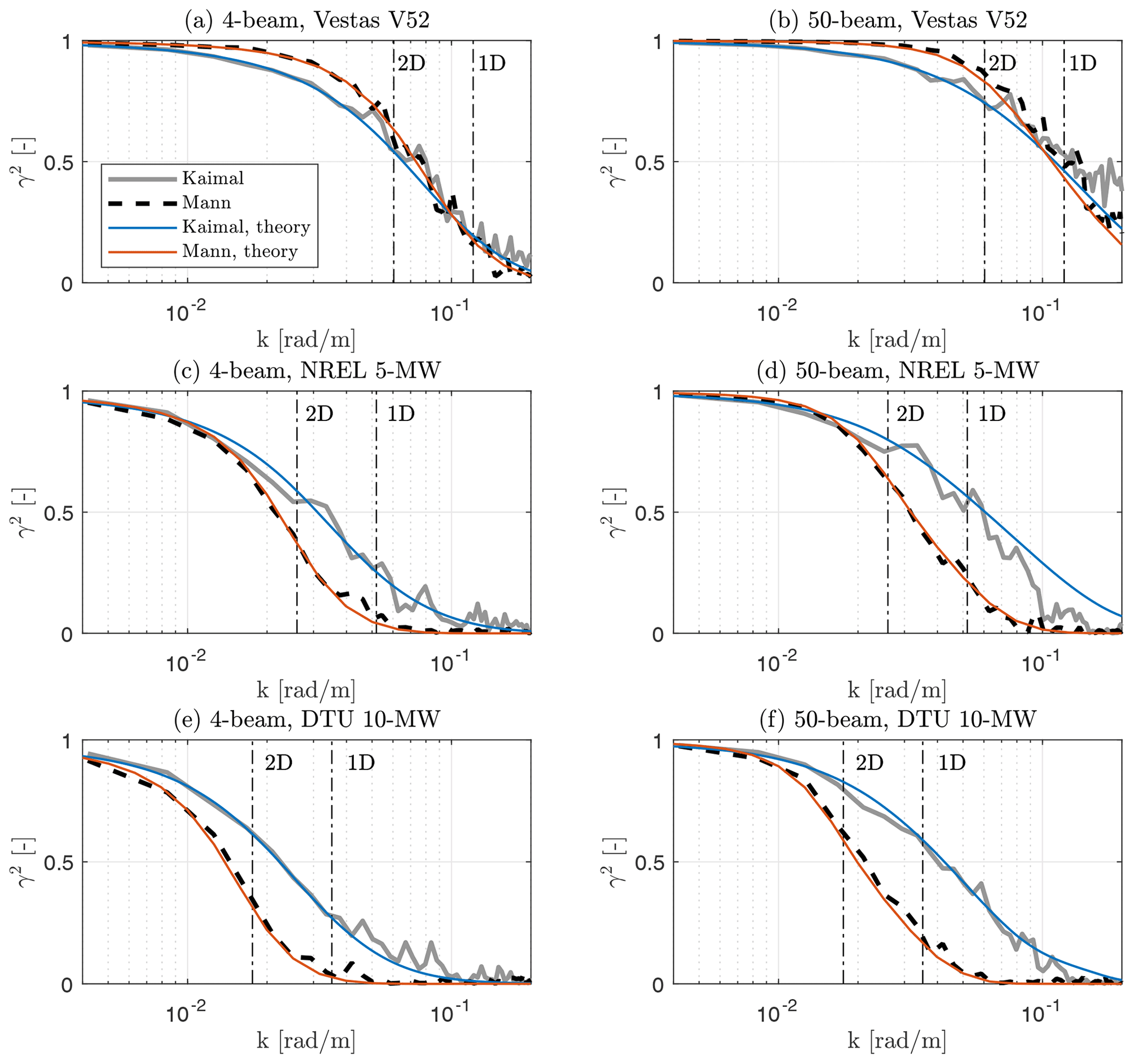
Figure 3Magnitude-squared coherence γ2 between lidar measurements and the REWS. Results (a, c, e) for the 4-beam scan pattern and (b, d, f) the 50-beam circular scan pattern. From top to bottom, the plots show results for the Vestas V52 turbine, NREL 5 MW turbine and DTU 10 MW turbine. The dash–dot lines labeled 1 and 2 D represent the wavenumbers and , respectively. In the legend, “theory” denotes the theoretical coherence.
The key findings of this study are included in the following discussion. For brevity, the magnitude-squared coherence with the Mann model is represented by , and the magnitude-squared coherence with the Kaimal model is represented by . Corresponding theoretical-coherence curves are also included in this figure following methods described in works by Held and Mann (2019) and Schlipf et al. (2013a).
-
For the Vestas V52 turbine in Fig. 3a and b, is higher than in the low-wavenumber region k≤0.06 rad m−1, which aligns with the findings of the work by Held and Mann (2019), in which the authors suggested that the Kaimal model gave a slight underestimation of the measurement coherence for a 52 m rotor diameter, and the coherence predicted from the Kaimal model is lower than the coherence predicted from the Mann model.
-
For the NREL 5 MW turbine in Fig. 3c and d, is slightly higher than for low wavenumbers. Then, the coherence starts to separate around 2 D. Specifically, decreases more sharply than when k exceeds 2 D.
-
For the DTU 10 MW turbine in Fig. 3e and f, the trend follows the trend with the NREL 5 MW turbine, but is considerably lower than . The coherence of drastically decreases before 2 D. For increasing wavenumbers, larger discrepancies are noticeable between and .
-
The additional measurement points with the circular scan provide an obvious improvement in measurement coherence in the frequency band . The maximum coherence bandwidth k0.5 can reach 1 D with the 50-beam circular scan. The Kaimal model indicates that the 50-beam circular scan is a better scan pattern and can lead to realizing the full potential benefits of lidar-assisted collective pitch control. Surprisingly, the maximum coherence bandwidth k0.5 with the Mann model is far below 1 D, which will lead to lower benefits during the wind turbine design phase.
A novel finding in this work is that the coherence with the Mann model is lower that with the Kaimal model for large rotors, and this difference becomes larger with increasing rotor size. Conversely, for small rotor sizes, the coherence with the Mann model is higher than that with the Kaimal model. The differences between and are significant. These results are in accord with the theoretical coherence shown in Fig. 2, indicating lower coherence with the Mann model for larger separation distances.
In summary, these results provide important insights into the impact of different turbulence models on lidar measurement coherence. If the wind conditions at a site agree more closely with the Mann model, the lower coherence with the Mann model will diminish the advantages of LAC because inappropriate blade pitch actions in response to the lidar measurements will deteriorate the turbine structural loading. It can therefore be suggested that the turbulence model needs to be carefully considered while integrating the LAC solution with larger-rotor turbine designs.
This work confirms the association between lidar measurement coherence, the turbulence model and rotor size. Our results suggest that this impact should be considered an uncertainty when evaluating the benefits of LAC during the wind turbine design phase. Note that the impacts on the load reduction need to be further investigated using reference turbines and aero-elastic tools following the IEC standards. More broadly, further research should be undertaken to provide guidelines on how to determine the optimal scan pattern for different site-specific atmospheric conditions and rotor sizes. Field validation is strongly recommended to mitigate the risk induced by site-specific wind conditions if LAC is adopted, especially for large rotors.
The turbulence box data could be made available on request.
LD was involved in the conceptualization of the project, the creation of the methodology, the use of software, the investigation and the writing of the original draft of this paper. WHL was involved in the conceptualization of the project, the creation of the methodology, the investigation and the writing of the original draft of this paper. ES was involved in the creation of the methodology, the investigation and the writing of the original draft of this paper.
The contact author has declared that neither they nor their co-authors have any competing interests.
The views expressed in the article do not necessarily represent the views of the DOE or the US Government. The US Government retains and the publisher, by accepting the article for publication, acknowledges that the US Government retains a nonexclusive, paid-up, irrevocable, worldwide license to publish or reproduce the published form of this work or allow others to do so for US Government purposes.
Publisher's note: Copernicus Publications remains neutral with regard to jurisdictional claims in published maps and institutional affiliations.
The authors want to thank Jakob Mann for providing the inputs of theoretical-coherence results with the Mann model and his suggestions on the manuscript.
This research was supported by the Energy Technology Development and Demonstration Program (EUDP) for the project “Lidar-assisted control for reliability improvement” (LICOREIM, grant no. 64019-0580).
This work was authored in part by the National Renewable Energy Laboratory, operated by Alliance for Sustainable Energy, LLC, for the US Department of Energy (DOE) under contract no. DE-AC36-08GO28308. Funding was provided by the US Department of Energy Office of Energy Efficiency and Renewable Energy Wind Energy Technologies Office.
This paper was edited by Joachim Peinke and reviewed by two anonymous referees.
Bak, C., Zahle, F., Bitsche, R., Yde, A., Henriksen, L. C., Natarajan, A., and Hansen, M. H.: Description of the DTU 10 MW Reference Wind Turbine, Tech. rep., DTU Wind Energy Report-I-0092, DTU Wind Energy, Roskilde, Denmark, 2013. a
Bossanyi, E.: Un-freezing the turbulence: application to LiDAR-assisted wind turbine control, IET Renew. Power Generat., 7, 321–329, 2013. a, b
Bossanyi, E., Kumar, A., and Hugues-Salas, O.: Wind turbine control applications of turbine-mounted LIDAR, J. Phys.: Conf. Ser., 555, 012011, https://doi.org/10.1088/1742-6596/555/1/012011, 2014. a
Chougule, A., Mann, J., Kelly, M., Sun, J., Lenschow, D. H., and Patton, E. G.: Vertical cross-spectral phases in neutral atmospheric flow, J. Turbulence, 13, N36, https://doi.org/10.1080/14685248.2012.711524, 2012. a
Eliassen, L. and Obhrai, C.: Coherence of Turbulent Wind under Neutral Wind Conditions at FINO1, in: Energy Procedia, vol. 94, Elsevier Ltd, Trondheim, Norway, 388–398, https://doi.org/10.1016/j.egypro.2016.09.199, 2016. a
Fleming, P. A., Scholbrock, A., Jehu, A., Davoust, S., Osler, E., Wright, A. D., and Clifton, A.: Field-test results using a nacelle-mounted lidar for improving wind turbine power capture by reducing yaw misalignment, J. Phys.: Conf. Ser., 524, 012002, https://doi.org/10.1088/1742-6596/524/1/012002, 2014. a
Haizmann, F., Schlipf, D., and Cheng, P. W.: Correlation-model of rotor-effective wind shears and wind speed for lidar-based individual pitch control, Proceedings of the Twelfth (2015) German Wind Energy Conference DEWEK, Bremen, Germany, https://doi.org/10.18419/opus-3976, 19–20 May 2015. a, b
Hansen, M. H., Henriksen, L. C., Tibaldi, C., Bergami, L., Verelst, D., Pirrung, G., and Riva, R.: HAWCStab2: User Manual, Tech. Rep. October, DTU Wind Energy, available at: https://www.hawcstab2.vindenergi.dtu.dk/ (last access: 24 November 2021), 2018. a
Held, D. P. and Mann, J.: Lidar estimation of rotor-effective wind speed – an experimental comparison, Wind Energ. Sci., 4, 421–438, https://doi.org/10.5194/wes-4-421-2019, 2019. a, b, c, d, e
IEC: Wind energy generation systems – Part 1: Design requirements, Tech. rep., International Electrotechnical Commission, Geneva, Switzerland, 2019. a, b, c, d, e, f
Jonkman, B. J. and Buhl Jr., M. L.: TurbSim user's guide, Tech. rep., Technical Report NREL/TP-500-39797, National Renewable Energy Laboratory, Golden, Colorado, USA, 2006. a
Jonkman, J., Butterfield, S., Musial, W., and Scott, G.: Definition of a 5 MW Reference Wind Turbine, Tech. rep., Technical Report NREL/TP-500-38050, National Renewable Energy Laboratory, Golden, Colorado, USA, 2009. a
Kumar, A. A., Bossanyi, E. A., Scholbrock, A. K., Fleming, P., Boquet, M., and Krishnamurthy, R.: Field Testing of LIDAR-Assisted Feedforward Control Algorithms for Improved Speed Control and Fatigue Load Reduction on a 600-kW Wind Turbine, Tech. rep., NREL – National Renewable Energy Lab., Golden, CO, USA, 2015. a
Mann, J.: The Spatial Structure of Neutral Atmospheric Surface-Layer Turbulence, J. Fluid Mech., 273, 141–168, https://doi.org/10.1017/S0022112094001886, 1994. a
Mann, J.: Wind field simulation, Probabil. Eng. Mech., 13, 269–282, https://doi.org/10.1016/s0266-8920(97)00036-2, 1998. a
Nybø, A., Nielsen, F. G., Reuder, J., Churchfield, M. J., and Godvik, M.: Evaluation of different wind fields for the investigation of the dynamic response of offshore wind turbines, Wind Energy, 23, 1810–1830, https://doi.org/10.1002/we.2518, 2020. a, b
Pena, A., Eds, C. B. H., Bischoff, O., Frandsen, S. T., Mann, J., and Trujillo, J. J.: Remote Sensing for Wind Energy, Tech. Rep. May, DTU Wind Energy, Roskilde, Denmark. No. 0084, available at: https://orbit.dtu.dk/en/publications/remote-sensing-for-wind-energy-4 (last access: 24 November 2021), 2015. a
Schlipf, D., Schuler, S., Grau, P., Allgöwer, F., and Kühn, M.: Look-ahead cyclic pitch control using lidar, in: Proceedings of the Science of Making Torque from Wind, Heraklion, Greece, 28–30 June 2010, https://doi.org/10.18419/opus-4538, 2010. a
Schlipf, D., Kapp, S., Anger, J., Bischoff, O., Hofsäß, M., Rettenmeier, A., and Kuhn, M.: Prospects of Optimization of Energy Production by LIDAR Assisted Control of Wind Turbines, in: EWEA 2011 conference proceedings, 1–10, Brussels, Belgium, available at: http://elib.uni-stuttgart.de/opus/volltexte/2013/8585/ (last access: 24 November 2021), 2011. a, b
Schlipf, D., Cheng, P. W., and Mann, J.: Model of the Correlation between Lidar Systems and Wind Turbines for Lidar-Assisted Control, J. Atmos. Ocean. Tech., 30, 2233–2240, https://doi.org/10.1175/JTECH-D-13-00077.1, 2013a. a, b, c
Schlipf, D., Schlipf, D. J., and Kühn, M.: Nonlinear model predictive control of wind turbines using LIDAR, Wind Energy, 16, 1107–1129, https://doi.org/10.1002/we.1533, 2013b. a, b
Schlipf, D., Fleming, P., Haizmann, F., Scholbrock, A., Hofsäß, M., Wright, A., and Cheng, P. W.: Field testing of feedforward collective pitch control on the CART2 using a nacelle-based lidar scanner, J. Phys.: Conf. Ser., 555, 012090, https://doi.org/10.1088/1742-6596/555/1/012090, 2014. a
Schlipf, D., Fürst, H., Raach, S., and Haizmann, F.: Systems Engineering for Lidar-Assisted Control: A Sequential Approach, J. Phys.: Conf. Ser., 1102, 012014, https://doi.org/10.1088/1742-6596/1102/1/012014, 2018. a, b, c
Scholbrock, A., Fleming, P., Schlipf, D., Wright, A., Johnson, K., and Wang, N.: Lidar-enhanced wind turbine control: Past, present, and future, in: IEEE 2016 American Control Conference (ACC), 6–8 July, Boston, MA, USA, 1399–1406, 2016. a
Simley, E. and Pao, L. Y.: A longitudinal spatial coherence model for wind evolution based on large-eddy simulation, in: IEEE 2015 American Control Conference (ACC), 1–3 July, Chicago, IL, USA, 3708–3714, 2015. a
Simley, E., Pao, L., Frehlich, R., Jonkman, B., and Kelley, N.: Analysis of wind speed measurements using continuous wave LIDAR for wind turbine control, in: 49th AIAA Aerospace Sciences Meeting including the New Horizons Forum and Aerospace Exposition, 4–7 January 2011, Orlando, Florida, USA, p. 263, 2011. a
Simley, E., Pao, L., Kelley, N., Jonkman, B., and Frehlich, R.: Lidar wind speed measurements of evolving wind fields, in: 50th AIAA aerospace sciences meeting including the new horizons forum and aerospace exposition, 9–12 January 2012, Nashville, Tennessee, USA, p. 656, 2012. a, b
Simley, E., Pao, L. Y., Frehlich, R., Jonkman, B., and Kelley, N.: Analysis of light detection and ranging wind speed measurements for wind turbine control, Wind Energy, 17, 413–433, https://doi.org/10.1002/we.1584, 2014. a, b
Simley, E., Fürst, H., Haizmann, F., and Schlipf, D.: Optimizing Lidars for Wind Turbine Control Applications – Results from the IEA Wind Task 32 Workshop, Remote Sens., 10, 863, https://doi.org/10.3390/rs10060863, 2018. a, b, c, d, e, f
Simley, E., Bortolotti, P., Scholbrock, A., Schlipf, D., and Dykes, K.: IEA Wind Task 32 and Task 37: Optimizing Wind Turbines with Lidar-Assisted Control Using Systems Engineering, J. Phys.: Conf. Ser., 1618, 042029, https://doi.org/10.1088/1742-6596/1618/4/042029, 2020. a
Veers, P. S.: Three-dimensional wind simulation, Tech. rep., Sandia National Labs., Albuquerque, NM, USA, 1988. a
- Abstract
- Introduction
- Preliminaries and evaluation of different turbulence models
- Modeling of lidar wind speed measurements
- Influence of different turbulence models on lidar measurement coherence
- Conclusions
- Data availability
- Author contributions
- Competing interests
- Disclaimer
- Acknowledgements
- Financial support
- Review statement
- References