the Creative Commons Attribution 4.0 License.
the Creative Commons Attribution 4.0 License.
 | 15 Mar 2021
Low-Reynolds-number investigations on the ability of the strip of e-TellTale sensor to detect the flow features over wind turbine blade section: flow stall and reattachment dynamics
Antoine Soulier
Caroline Braud
Dimitri Voisin
Bérengère Podvin
Monitoring the flow features over wind turbine blades is a challenging task that has become more and more crucial. This paper is devoted to demonstrate the ability of the e-TellTale sensor to detect the flow stall–reattachment dynamics over wind turbine blades. This sensor is made of a strip with a strain gauge sensor at its base. The velocity field was acquired using time-resolved particle image velocimetry (TR-PIV) measurements over an oscillating 2D blade section equipped with an e-TellTale sensor. PIV images were post-processed to detect movements of the strip, which was compared to movements of flow. Results show good agreement between the measured velocity field and movements of the strip regarding the stall–reattachment dynamics.
- Article
(14495 KB) - Full-text XML
- BibTeX
- EndNote


Wind turbines are placed in the low layers of the atmospheric boundary layer where the wind is strongly influenced by the surface roughness and the thermal stability which creates turbulence and vertical gradients of the wind (Emeis, 2018). The rotor yaw and the blade pitch alignment within this highly unsteady wind inflow are a subject that is becoming more and more crucial with rotor blade lengths that are increasingly long (107 m for the largest existing turbine: Haliade-X). Also, offshore turbines are arranged in an array layout and not just in line, which induces additional sheared inflow conditions and additional small turbulent structures (Chamorro et al., 2012). This results in strong and local variations in speed and directions on the wind turbine rotor blades. These variations lead to unsteady aerodynamic effects with turbulent inflows responsible for more than 65 % of fatigue loads (Rezaeiha et al., 2017). To alleviate these loads, smart blades and/or fluidic actuators are now considered (Pechlivanoglou, 2013; Jaunet and Braud, 2018; Batlle et al., 2017). For this last strategy or to perform blade remote monitoring, one key issue is the development of robust technologies able to provide an instantaneous detection of the state of the flow on the blade aerodynamic surface. On current operating wind turbines the wind is generally monitored using an anemometer situated on the nacelle. It provides a slow measure of the wind which is perturbed by the rotor and the nacelle. Moreover being only a one-point measurement, it does not appreciate shear, yaw/pitch misalignment or turbulence on blades. Other monitoring technologies allow some of these drawbacks to be overcome. Among the most mature technologies, the spinner anemometer measures the wind in front of the rotor, removing perturbations from the rotor (Pedersen et al., 2007). Also, capabilities, costs and integration of nacelle-mounted lidar, measuring the wind inflow a few diameters upstream of the rotor, has been significantly improved in the last decades (Aubrun et al., 2016; Bossanyi et al., 2014). However, to the knowledge of the authors, nothing is yet able to measure the state of the flow on current blades. Some field measurement campaigns were punctually performed for research purposes using pressure probes around dedicated manufactured blades. However the potential for using these sensors in a day-to-day operation of wind turbines is weak (Troldborg et al., 2013). Some solutions were explored such as tufts or stall flags glued to the blade correlated with positions of the flow separation (Swytink-Binnema and Johnson, 2016; Pedersen et al., 2017; Corten, 2001). However, these methods need a mounted camera on the turbine with its associated drawbacks (fragility of the camera, vision at night, etc.).
An interesting alternative to these technologies is the e-TellTale sensor, developed by Mer Agitée https://www.meragitee.com/ (last access: 11 February 2020). It is composed of a strip moving like a tuft but with a strain gauge encased in its base, making it able to transmit the information directly to any monitoring or control system through an embedded wireless electronic unit. It was originally developed to detect flow separation on sails of offshore racing sailing vessels and has been recently adapted for wind turbine blade monitoring. Robustness and practical mounting issues were solved from industrial tests (Fig. 1a), while full-scale tests of the device were performed at high Reynolds numbers in the NSA wind tunnel facility of CSTB (http://www.cstb.fr/fr/, last access: 11 February 2020), to demonstrate the relation between the e-TellTale sensor signal and the lift curve for different angles of incidence as can be seen in Fig. 1b (Soulier et al., 2017). It was found in particular that an e-TellTale sensor located at the trailing edge of the profile with a sufficiently long strip is able to detect both the trailing edge separation and the stall phenomena.
The present study is intended to study the ability of the e-TellTale sensor to dynamically detect the apparition of stall or reattachment processes and to distinguish one from the other. For that purpose, experiments of a downscaled 2D blade section, oscillating around the stall angle, were performed in the LHEEA aerodynamic wind tunnel, using time-resolved PIV and different post-processing methods to extract the strip position of the sensor in the flow field (vision algorithms) and to evaluate instants at which the stall–reattachment phenomenon occurs over the aerodynamic surface. Regarding this phenomenon, “attached” is used to designate the state in which the flow is attached at least at the leading edge but it may be detached at the trailing edge. The objective of the e-TellTale sensor is to detect the apparition of stall–reattachment for real-time monitoring or control purposes. Therefore, the detection methods used to validate this sensor preferably use instantaneous criteria: an instantaneous evaluation of the sign of the tangential velocity an instantaneous evaluation of the profile wake width. Only one statistical approach is chosen (POD decomposition).
The experimental setup and the post-processing methods are described in Sects. 2 and 3, respectively. Results are presented in Sect. 4 including a description of the baseline flow (Sect. 4.1) and results of the different post-processing methods to detect the flow stall–reattachment phenomena (Sect. 4.2), results on the ability of the e-TellTale sensors to detect flow separation (Sect. 4.3).
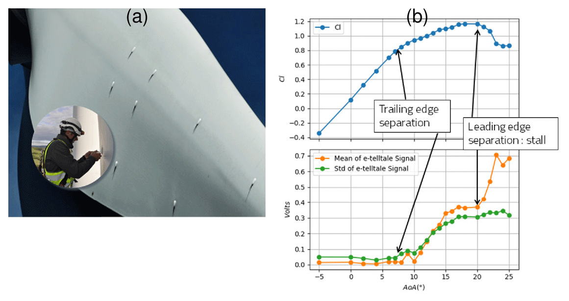
Figure 1Previous studies. (a) Robustness and practical mounting issues solved on EDF Renewables wind turbines. (b) Ability of full-scale e-TellTale sensors located at the blade trailing edge to detect static flow separations at high chord Reynolds numbers (106) from wind tunnel tests: increase in the e-TellTale signal after stall angle, at 20∘.
The experiments were performed in the recirculating aerodynamic wind tunnel facility of the LHEEA laboratory at Centrale Nantes (France). The working section is 0.5×0.5 m2 and 2.4 m long with a turbulent intensity less than 0.3 % of turbulence. The Reynolds number based on the chord length of the 2D blade section, c≃0.09 m, is with U∞=35 m/s as the free-stream velocity.
2.1 Blade profile
Measurements were performed using a NACA 654-421 profile in composite material. Due to the fabrication process, it is truncated at 91 % of the chord length so that the trailing edge thickness is 2 mm (see Fig. 2). A similar profile was already used by Jaunet and Braud (2018) to demonstrate the ability of local micro-jets to alleviate loads. It is a thick profile with two drops on the lift coefficient curve corresponding to a first boundary layer separation at the trailing edge of the profile for angle of attack (AoA) and a second flow separation at the leading edge for AoA causing stall. From 8 to 20∘ the separation point moves gradually from the trailing edge to the leading edge, corresponding to a gradual variation in the loads.
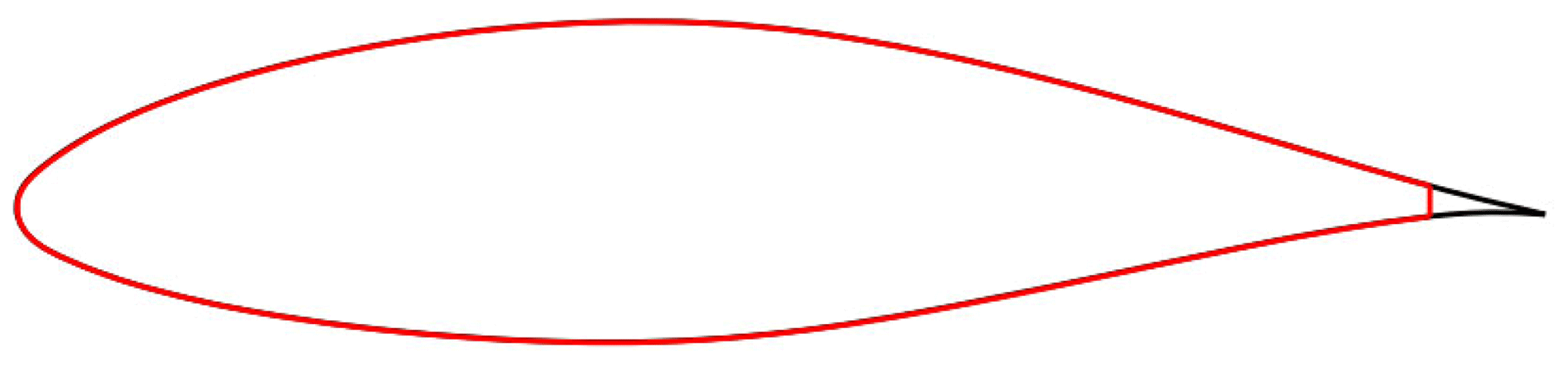
Figure 2NACA 654-421 profile manufactured in red and the theoretical trailing edge in black.
An oscillating motion was imposed using a crank drive for the linear movement imposed by a feedback linear motor from LinMot. This oscillating motion was checked from PIV image processing using the detection of the blade surface at the position of the e-TellTale sensor. The detection of the blade surface was also later used to extract the position of the e-TellTale sensor in the vector field (see Sect. 3.1) and will give information on the relative angle of incidence. The amplitude of the blade oscillation, , was chosen so that the flow, initially separated at the trailing edge, moves gradually towards the leading edge flow separation where the stall occurs as it can be checked on PIV vector fields in Figs. 8 and 9. The oscillating frequency, fosc=1 Hz, was chosen similar to the study of Jaunet and Braud (2018) to mimic a constant shear inflow. This leads to a reduced frequency of corresponding to a quasi-steady stall behavior (Choudhry et al., 2014). The blade was equipped with an e-TellTale sensor at mid-span on the suction side. Figure 3b shows the e-TellTale on the surface of the 2D blade profile installed in the LHEEA aerodynamic wind tunnel. A small part (≃5 mm) of the pink strip of the e-TellTale sensor is glued to a strain gauge sensor, itself glued on a thin stainless-steel sheet embedded in the blade. The rest of the strip is free to move above the aerodynamic surface. Its length is one-third of the blade chord. The signal from the strain gauge sensor was not acquired simultaneously during PIV measurements; however, it has been checked before experiments that the signal from this strip, made of a nylon fabric, behaves similarly to full-scale experiments from Soulier et al. (2017). In particular it was checked that it was possible to distinguish the first rise of the e-TellTale signal when the increasing angle of attack reaches the angle of trailing edge separation and then the sudden increase in the e-TellTale signal at the stall angle (see Fig. 1b). Also, no load measurements were performed during PIV measurements; thus only the spatiotemporal information will be used later to detect the stall state on the aerodynamic surface.
2.2 PIV measurements
Flow data were collected with a TR-PIV system able to produce 1600 velocity fields each second. A DM20-527 DH laser from Photonics Industries delivering a 2×20 mJ double laser sheet at the green wavelength of 527 nm was used in this setup. The camera was a Phantom Miro M310, recording 1200×800 px2 images at 3200 Hz; the 6 Gb of RAM memory of the camera allowed the capture of 2000 velocity fields for each run. The camera was equipped with a Zeiss Makro Planar lens (i.e. f=50 mm, ). With this setup, the field of view was 216×106 mm2, leading to a spatial resolution of 6.3 px/mm. The PIV velocity fields were computed using a 16×16 px2 interrogation area with an overlap of 50 %, leading to 159×99 vectors with a maximum spacing between vectors of 1.3 mm or 0.014 c. As seen in Fig. 3 the optical axis of the camera was not totally perpendicular to the laser sheet. After calibrating this misalignment by taking snapshots of a calibration target located at the measurement plane, all the raw images and the velocity fields were dewarped. In addition to the classical noise inherent to PIV measurement, the presence of the e-TellTale strip in the field of view of the PIV camera caused some spurious vectors explained by some light shoots on images when the clear fabric of the strip reflected the laser light directly towards the camera. To remove and replace these spurious vectors, the automated post-processing algorithm developed by Garcia (Garcia, 2011) was used. Figure 3 presents the framework (x, y, z) which is stationary in the wind tunnel.

Figure 3Experimental setup in the LHEEA wind tunnel: (a) scheme of the PIV setup with the framework of the axis (x, y, z). (b) The 2D blade section mounted in the test section with the e-TellTale sensor in pink.
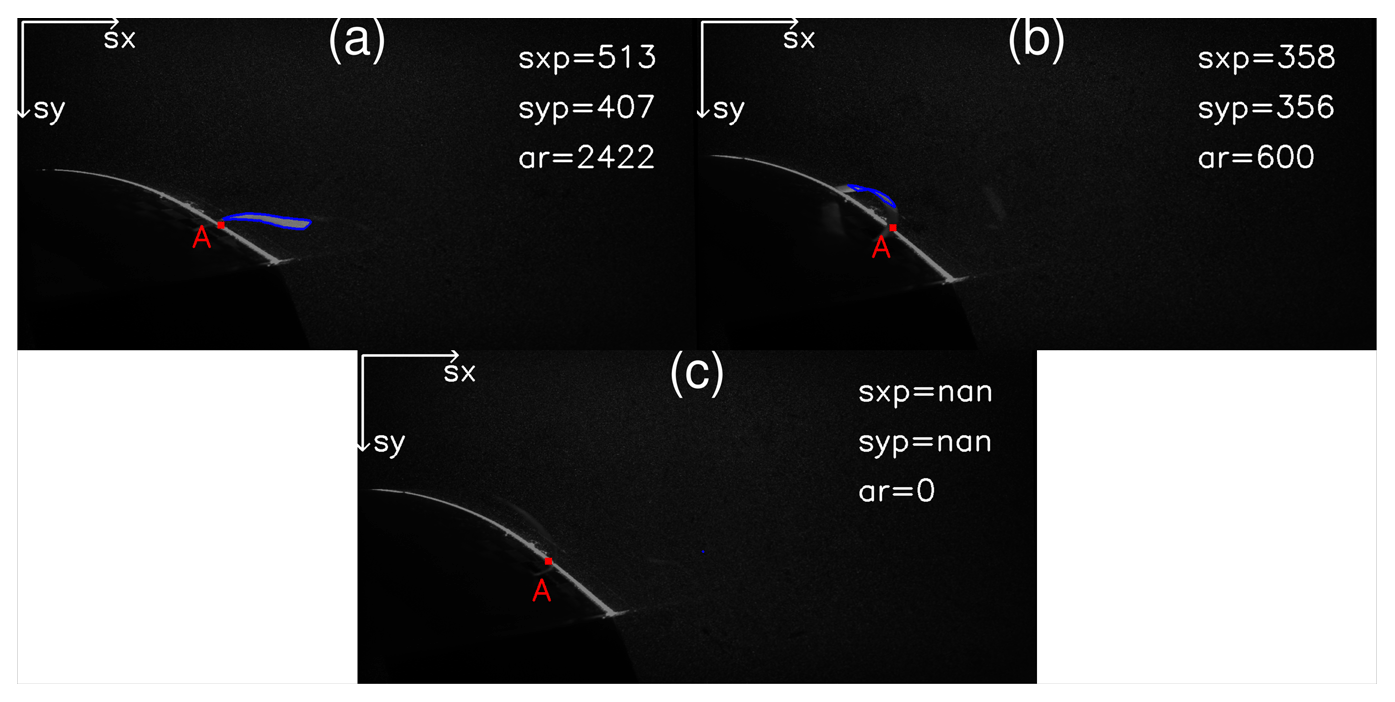
Figure 4Detected strip contour from PIV images using OpenCV: (a) for the attached flow case and (b) for the detached flow case (c) corresponding to an outlier case (impossible to detect the strip position). sxp and syp are respectively the streamwise and spanwise positions in pixels of the center of the detected area (in blue). ar is the area of the detected contour in pixels. The e-TellTale sensor is attached to the wall in A.
3.1 Strip detection method
The flow field over the aerodynamic surface is measured using TR-PIV measurements during the oscillations of the blade profile. To extract movements of the e-TellTale strip within this flow field, PIV images were post-processed using vision algorithms from the Open Source Computer Vision Library (OpenCV) https://opencv.org (last access: 11 February 2020).
The chosen methodology uses PIV images containing laser reflections of the blade surface and of the strip. The first step is to separate the blade surface contour from the strip contour. The images were first binarized so that white pixels, corresponding to the reflection of the laser on the blade and the strip surfaces, are set to 1 and all others to 0. To separate pixel coordinates of the blade from pixel coordinates of the strip, a local gradient of white pixel coordinates is computed, revealing ordinates of pixels corresponding to the strip location. Then, the resulting curve was smoothed using a Savitzky–Golay filter. Finally, this resulting identified profile curve was fit to the theoretical suction side profile curve to extract the best Euclidean transformation (i.e. only rotation, translation and uniform scaling considered for the transformation) going from the measured curve to the theoretical profile. This was done using a function of OpenCV which primarily uses the RANSAC algorithm to detect spurious points and then the Levenberg–Marquardt algorithm to fit the profile. The result is a transformation matrix from which an angle of rotation is extracted. Also, from the detected blade surface contour, a mask is defined to remove everything below it so that the remaining bright contour is the strip. The resulting cleaned binarized images were then used to extract the strip location using a contour detection function from OpenCV. The contour detection function recognizes the white pixels surrounded by other white pixels and regroups all of it in one entity. As we are interested in the flow separation phenomenon over the aerodynamic surface which induces large movements of the strip from the downstream to the upstream flow directions, it was found sufficient to summarize the position of the strip by the center position of the detected contour. The strip detection method was first validated on some samples such as in Fig. 4, which shows raw PIV images on which the detected area is circled in blue with the coordinate of its center denoted sxp and syp, in pixels, for the respective streamwise and normal directions. It was then possible to automatize the method for images of the oscillating blade periods. sxp then was adimensionned and became sx:
During the stall there are many more movements of the strip out of the plane of the laser sheet. In those cases, the strip was not lit up, and this results in a missing value in sxp as can be seen in Fig. 4c. These values were replaced by the minimum value of sx. The corrected signal, sxc, is presented with the original signal sx in Fig. 5.
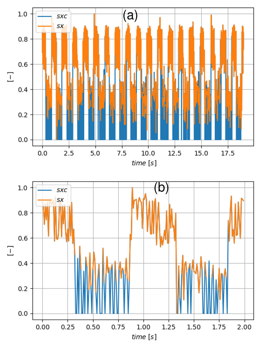
Figure 5Streamwise coordinate of the identified strip sx before correction and sxc after correction: (a) the full run and (b) a zoom on the two first oscillations.
3.2 Vortex identification method
Vortex identification methods are widely spread in the literature (see e.g., Jeong and Hussain, 1995). As they enable us to distinguish swirling motion from shearing motion, they were developed to help in the understanding of turbulent flows and more recently as a real-time processing method for flow control purposes (see e.g., Braud and Liberzon, 2018). In the present study, the Γ1 criterion method is used (Michard et al., 1997). This is a geometrical criterion defined as follows:
where N is the number of points M of the square area S around the center point P, UM the velocity at the point M and z the normal unit vector. The size of S acts as a spatial filter. For this study different sizes of S from 9×9 to 3×3 grid points were tested, and the differences were found to not be significant. The presented results were obtained with S being a square of 7×7 points. From this definition, Γ1 is a dimensionless scalar ranging from −1 to 1, for which the local extremum indicates the center of a vortex. Compared to other methods such as the well-known Q criterion, the Γ1 criterion provides equivalent results, with the advantages of avoiding computation of gradients (i.e. decreasing noise sensitivity) and providing the sign of vortices. Similar to Mulleners and Raffel (2013), the vortex identification method was used to extract vortex locations in the shear areas over the blade surface during the blade oscillation cycles (see Fig. 6 for an illustration of an instantaneous Γ1 field).
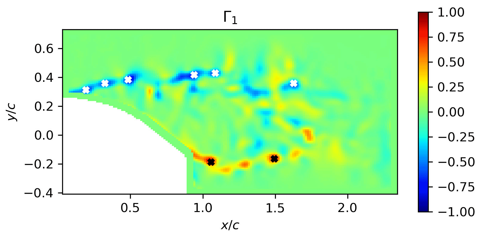
Figure 6Example of an instantaneous isocontour map of the Γ1 field with peaks identified using white cross markers for clockwise vortices and black cross markers for counterclockwise vortices.
3.3 Proper orthogonal decomposition
Proper orthogonal decomposition (POD) is a statistical technique (Holmes et al., 1996) that extracts spatial modes that are best correlated on average with a given field defined on a domain Ω. Let denote the temporal average. The field can be written as a superposition of spatial modes whose amplitude varies in time:
The modes can be identified with the method of snapshots (Sirovich, 1987), which is based on the computation of the temporal autocorrelation C for a given set of N snapshots :
where represents the fluctuating part of the snapshots ( ). The temporal amplitudes are eigenfunctions of
They are uncorrelated and their variance is given by
The spatial modes are then obtained from
By construction, the modes are orthonormal
POD was applied to the 2D ePIV vector fields over two different domains. The largest domain is used in the description of the baseline flow (Sect. 4.1), while the smaller domain is used to detect the flow stall–reattachment dynamics in the oscillating cycle (see Sect. 3.1).
Results are presented in three steps. Firstly, the baseline flow obtained with an oscillation frequency of the blade fosc=1 Hz and an acquisition frequency fPIV=100 Hz is described, including a description of the flow during an oscillation cycle and the description of the secondary oscillation in the wake flow when separated. From this PIV field visualization, a first evaluation of the stall–reattachment instants is performed and called the visual reference. Secondly, three methods to detect the flow stall–reattachment instants from PIV measurements are presented and compared. Thirdly, results of the detection of the strip are compared to all detection methods to evaluate the ability of the sensor to detect the flow stall–reattachment dynamic.
4.1 The baseline flow
One period of the blade oscillation relative angle, Δα, is extracted using the blade contour mask from PIV images as explained in Sect. 3.1 (see Fig. 7). The time duration T and the amplitude of the blade oscillation were chosen to include the flow separation phenomena for quasi-static stall conditions, as previously described in Sect. 2.1. Points of interest within this oscillating period are marked with letters from (a) to (i), and the corresponding instantaneous vector fields are presented in Figs. 8 and 9. At the beginning of the oscillating period, Δα=0∘ and , the flow is slightly separated at the trailing edge of the profile as can be seen in Fig. 8a. From points (a) to (c), corresponding to a positive blade incidence variation, the separation point moves gradually from the trailing edge to the leading edge of the profile, and the wake width increases accordingly as illustrated from Fig. 8a to b. From point (c) to point (d) the separation point suddenly moves towards the leading edge with a corresponding massive increase in the wake width, until the flow is fully separated over the aerodynamic profile (see Fig. 8c and d). This last phenomenon is 10 times faster than the previous one and is clearly related to the stall phenomenon. From point (d) to point (e), the flow after the blade can clearly be considered as an asymmetric wake flow with shear layers on both sides of the blade (see Fig. 8d and e).
From points (e) to (g), despite the progressive decrease in the adverse pressure gradient (Devinant et al., 2002) on the suction side of the blade through a negative variation in the blade incidence during 0.3 s, the flow remains fully separated (see Fig. 9e, f and g). From point (g) to point (h), corresponding to a duration of Δt=0.02 s, the separation point suddenly moves back towards the trailing edge; thus it is the reattachment. Again, this phenomenon is 10 times faster than the time duration from (e) to (g) for which the blade incidence is progressively decreasing (see Fig. 9g and h). From points (h) to (i), the separation point is back to its initial state (see Fig. 9h and i). This is the first visual method to detect the stall and reattachment instants, defined respectively as and , with tc, td, tg and th the instants (c), (d), (g) and (h) extracted from ic=1 to Ncycle, Ncycle=18 being the total number of instantaneous oscillation cycles. They will be used in the following sections as a comparison for the flow stall–reattachment detection methods of Sect. 4.2.
It should be emphasized that the stall–reattachment phenomena has a timescale corresponding to in good agreement with the theoretical work of Jones (Jones, 1940), with a stall–reattachment location occurring within one-third of the blade chord from the leading edge.
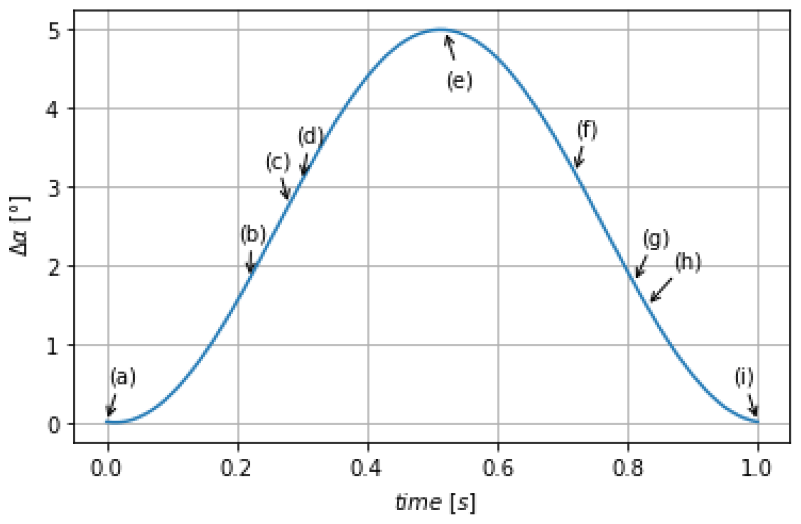
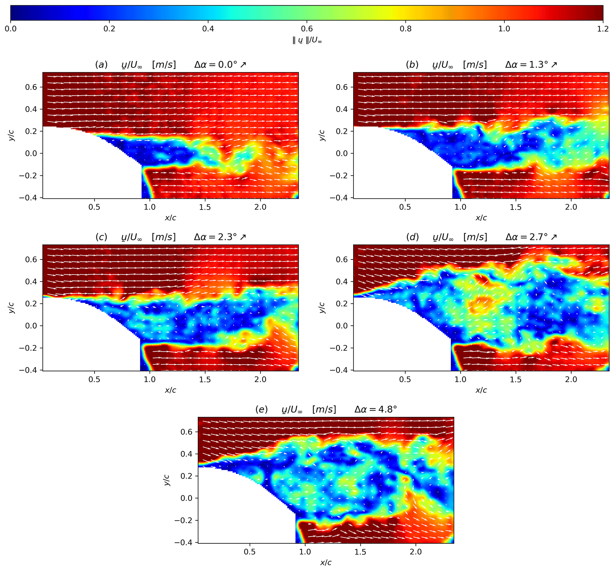
Figure 8Instantaneous velocity fields superposed with isocontours of the velocity modulus (i.e. ) at different Δα values corresponding to points of the blade oscillation given in Fig. 7 during the upstroke phase (noted ↗): (a) is a point at the lowest Δα of the upstroke phase of the oscillation cycle, (b) is an intermediate point, (c) is a point just prior to stall, (d) is a point just after the stall and (e) corresponds to a point at the maximum amplitude of the blade oscillation cycle.
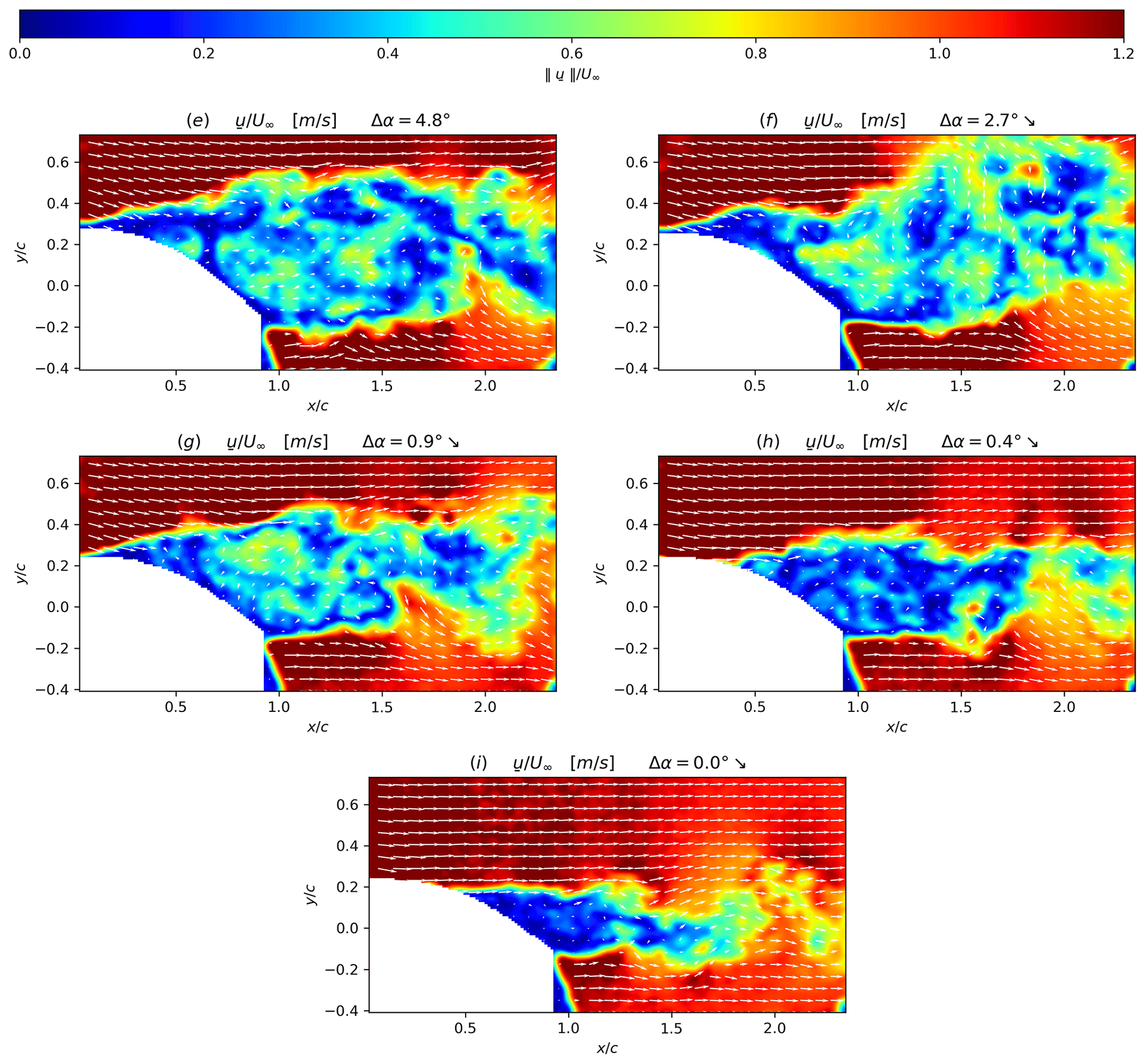
Figure 9Instantaneous velocity fields superposed with isocontours of the velocity modulus (i.e. ) at different Δα values corresponding to points of the blade oscillation given in Fig. 7 during the downstroke phase (noted ↘): (e) corresponds to a point at the maximum amplitude of the blade oscillation cycle, (f) is an intermediate point, (g) is a point just prior to the flow reattachment, (h) is a point just after the flow reattachment and (i) is a point at the lowest Δα of the downstroke phase.
To further characterize the coherent structure organization during this blade oscillation cycle, a POD analysis is performed from a database coming from a higher PIV acquisition rate, fPIV=1600 Hz. All vector fields of the blade oscillation cycles are used for the computation of the temporal autocorrelation coefficient C (see Sect. 3.3), corresponding to 2000 snapshots. The convergence of the resulting POD decomposition, in terms of the relative energy content with modes, is presented in Fig. 10 using the following definition:
where N is the number of modes and λi the eigenvalue of the ith mode.

As highlighted from Fig. 10, the dominant modes in terms of energy content are the first three POD modes, with around 14 % of kinetic turbulent energy for the first mode, 10 % for mode 2 % and 8 % for mode 3. These three modes are represented in Fig. 11 using the spatial modes, with , together with the temporal modes scaled with the associated energy content, with . The first mode is phased with the blade oscillation period and clearly captures variations in the mean velocity deficit in the wake due to these oscillations. The second and third modes exhibit structures in the wake which could be associated with the vortex shedding organization, typically found in the wakes of bluff bodies. Following the work of Yarusevych et al. (2009), the Strouhal number is extracted, with fs the peak frequencies from the fast Fourier transform (FFT) of temporal modes, with , and d a measure of the wake width using the vertical distance between the two local maximum of the rms of the streamwise velocity at . This Strouhal number is of the same order of magnitude as the one found by Yarusevych et al. (2009) behind the wake of a NACA 0025 airfoil at the angle of attack of 10∘, and the value above 0.2 is consistent with what was found on cylinders (see Norberg, 2003). The Strouhal number clearly assess the link of these modes to the vortex shedding organization behind the blade wake (see Fig. 12).
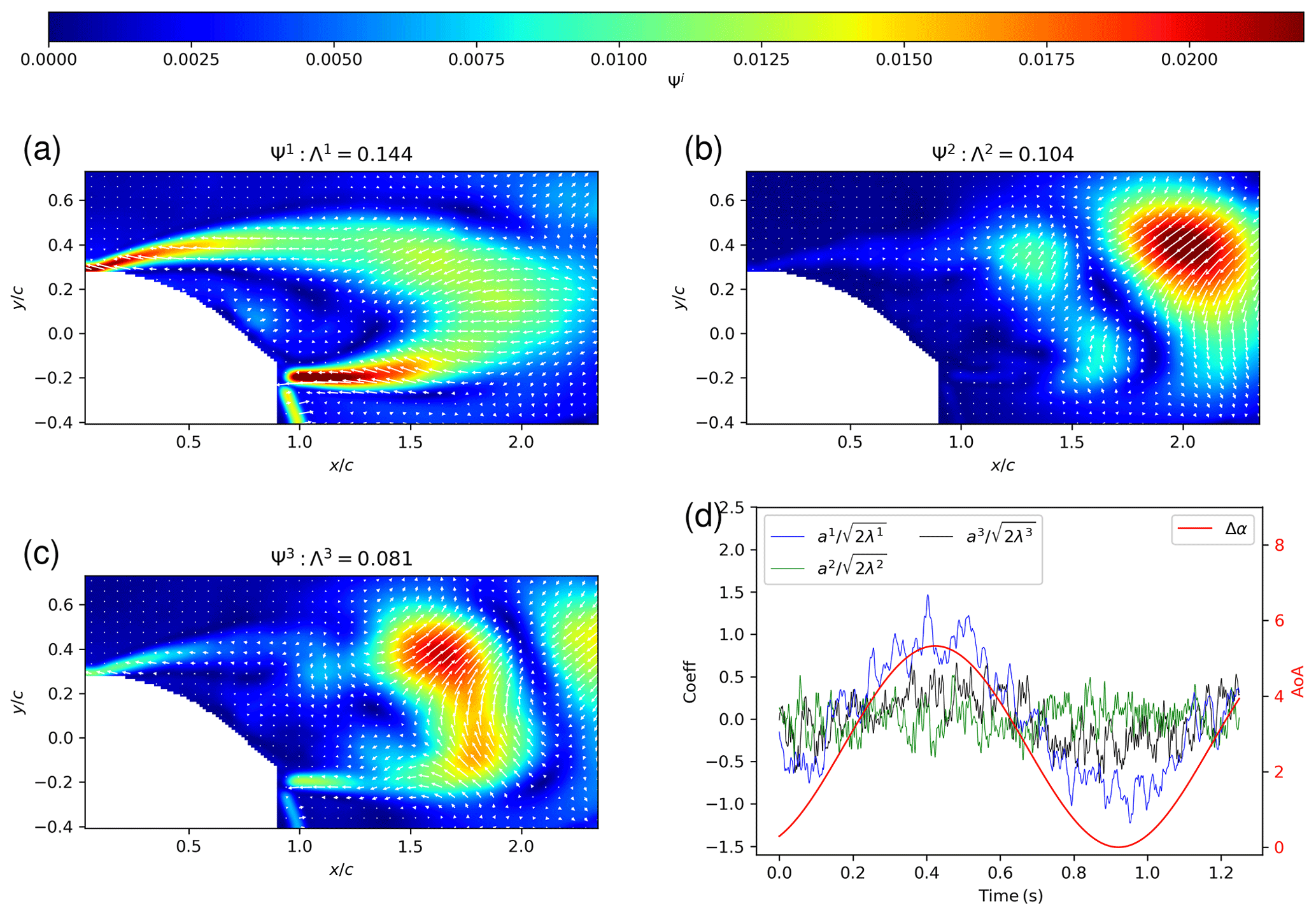
Figure 11POD decomposition. Panels (a), (b) and (c) represent the eigenvector vector field, , of the first three modes respectively () with isocontours of its modulus superimposed. The associated energy content of the nth mode (i.e. Λn) is written in the title; (d) represents the corresponding temporal coefficients scaled with their energy content.
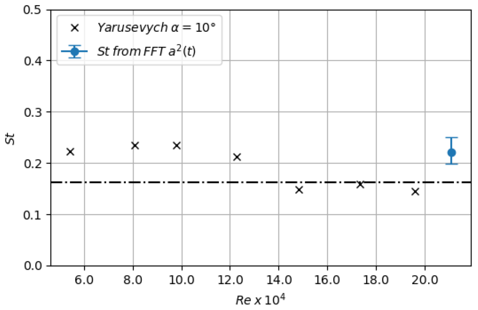
Figure 12Strouhal number values extracted from Yarusevych et al. (2009) and from the FFT of the temporal mode, a2(t), of the POD decomposition.
4.2 Detection methods
To be able to study the ability of the strip to detect the instants of the flow stall–reattachment phenomena, it was necessary to use some methods allowing the detection of these flow characteristics from PIV velocity fields. Several methods were identified from the literature, but as no comparison was found three existing methods were adapted to the specific needs of this study, and they were compared between each other to provide a more exhaustive detection from the PIV fields.
-
Method 1. Use the sign of the instantaneous tangential velocity component in the direction perpendicular to the surface as introduced by De Gregorio et al. (2007).
-
Method 2. Use the instantaneous detection of the wake width from extraction of vortices in the shear layers as explained in Sect. 3.2.
-
Method 3. Use the first mode of the POD decomposition introduced in Sect. 3.3.
From the perspective of using these sensors for real-time control/monitoring purposes, the application of methods 1 and 2 to the instantaneous PIV vector fields is preferred.
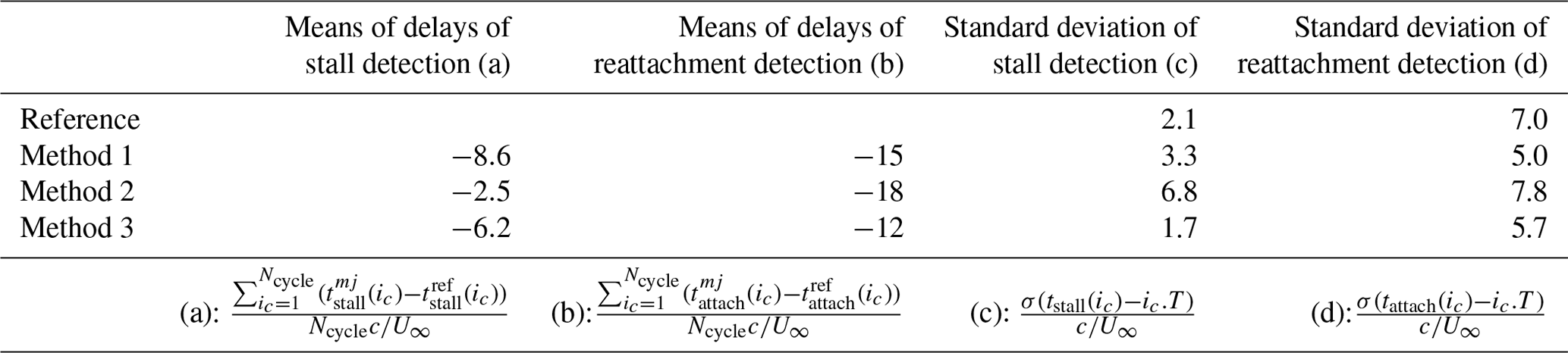
Table 1Summary of detected stall–reattachment instants using the three methods including the reference case. All times are expressed as chord times .
4.2.1 Method 1
For the first method, the apparition of stall–reattachment phenomena is detected using the normal profile of the instantaneous streamwise (direction of U∞) velocity component at a position corresponding to the attached strip location , , with t the timestamp of the snapshot and yb the direction normal to the blade surface. The chosen line location is presented in white in Fig. 13. The normal profile is then reduced to a single value by averaging in the normal direction, , with the normalized integration length in the normal direction, chosen so that each instant (or each angle of incidence) corresponds to one value of this normal velocity.
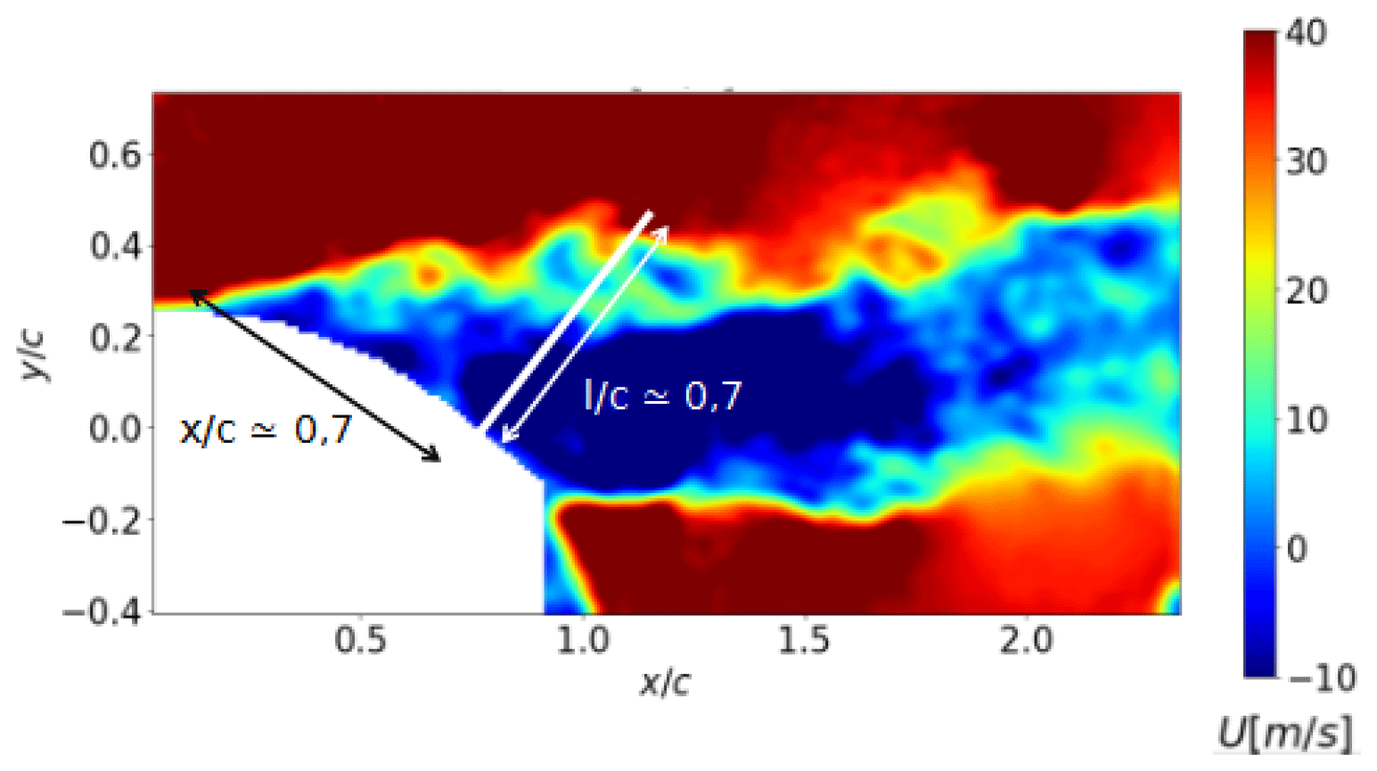
Figure 13First method to detect the flow stall–reattachment instants: location and direction of integration line used to compute Unorm(t) (i.e. white bar on the blade) reported on isocontours of the velocity modulus from PIV measurements.
The phased average of the obtained Unorm(t,xstrip) signal, , is presented in Fig. 14a for different values of together with its time derivative and with hatched time windows for which width, marked by green and red hatched areas, corresponds to the standard deviation centered on the average of the reference instants extracted from the visualization of instantaneous velocity fields of Sect. 4.1, and .
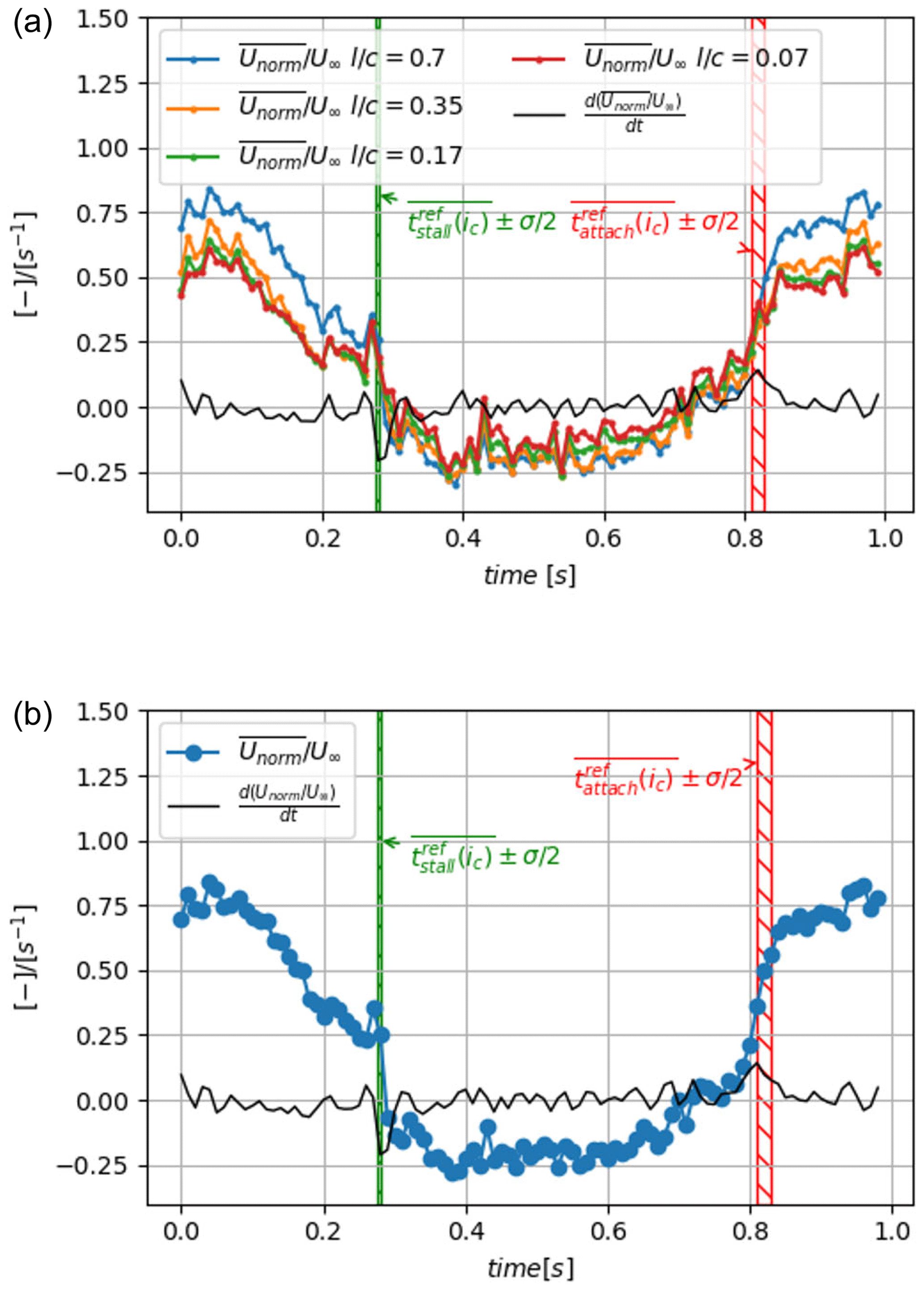
Figure 14The phased-averaged signal of the first detection method with its time derivative : (a) for different values of and (b) for .
For low angles of incidence , meaning is close to the free-stream velocity, which corresponds to an attached flow state over the aerodynamic surface. Similarly, for the large angles of incidence, is negative, bringing to light the reverse flow above the profile and thus the flow separation state. Between and , the instantaneous vertical profiles contain reverse flow but not enough on average to be fully separated. The flow can be considered stalled or reattached if presents a peak of the time derivative. Interestingly, whatever the value of , the location of the timestamp and the slope of at the peak of time derivative are not modified. In the following, is chosen (see Fig. 14a), which enables us to have a higher amplitude and thus a better signal-to-noise ratio to detect the gradients. Moreover, it is of the order of magnitude of the average recirculation region width in the normal direction. Time derivative peaks of the signal are close to these visual reference instants, within plus or minus one time step, which constitute a first validation of the method. It is interesting to note that the stall phenomenon is marked by a rapid and strong modification of the value from 0.25 to 0, while the reattachment phenomenon is smoother. This trend is also observed in other methods through a larger dispersion of the detected instants (see Table 1).
In wind tunnels, it is possible to reproduce known oscillations of the blade incidence to perform phase-averaged treatments on signals as shown in Fig. 14. However, the targeted objective of e-TellTale sensors is to detect flow separations on operating wind turbines, without any inflow measurement or real-time control. It is thus of interest to explore detection methods from the instantaneous signals. As shown in Fig. 15, the raw signal Unorm(t,xstrip) needs to be smoothed in order to detect a unique stall and reattachment instant. Smoothing instantaneous signals is a standard process to remove noise in real-time control applications; however, in turbulent flow signals, this is equivalent to filtering the smallest turbulent structures and thus obtaining an ensemble average more or less biased (Cahuzac et al., 2010). The centered moving-average algorithm is chosen here for its simplicity of implementation. For this treatment a filter size which will be unique for the sake of comparison with other detection methods needs to be defined. The main bias of this smoothing procedure is to reduce the slope as illustrated in Fig. 15. Because of the modification of the slope, constant bias is introduced in the detected instants, and it also depends on the threshold values used. Larger filter size has a larger impact on the slopes; however, a filter size as high as c=21 time steps was found necessary to have an automatic procedure to extract stall and reattachment instants for all detection methods and thus have comparable results. The bias introduced with the chosen threshold (zero-crossing) is presented in Table 1 in Sect. 4.2.4.
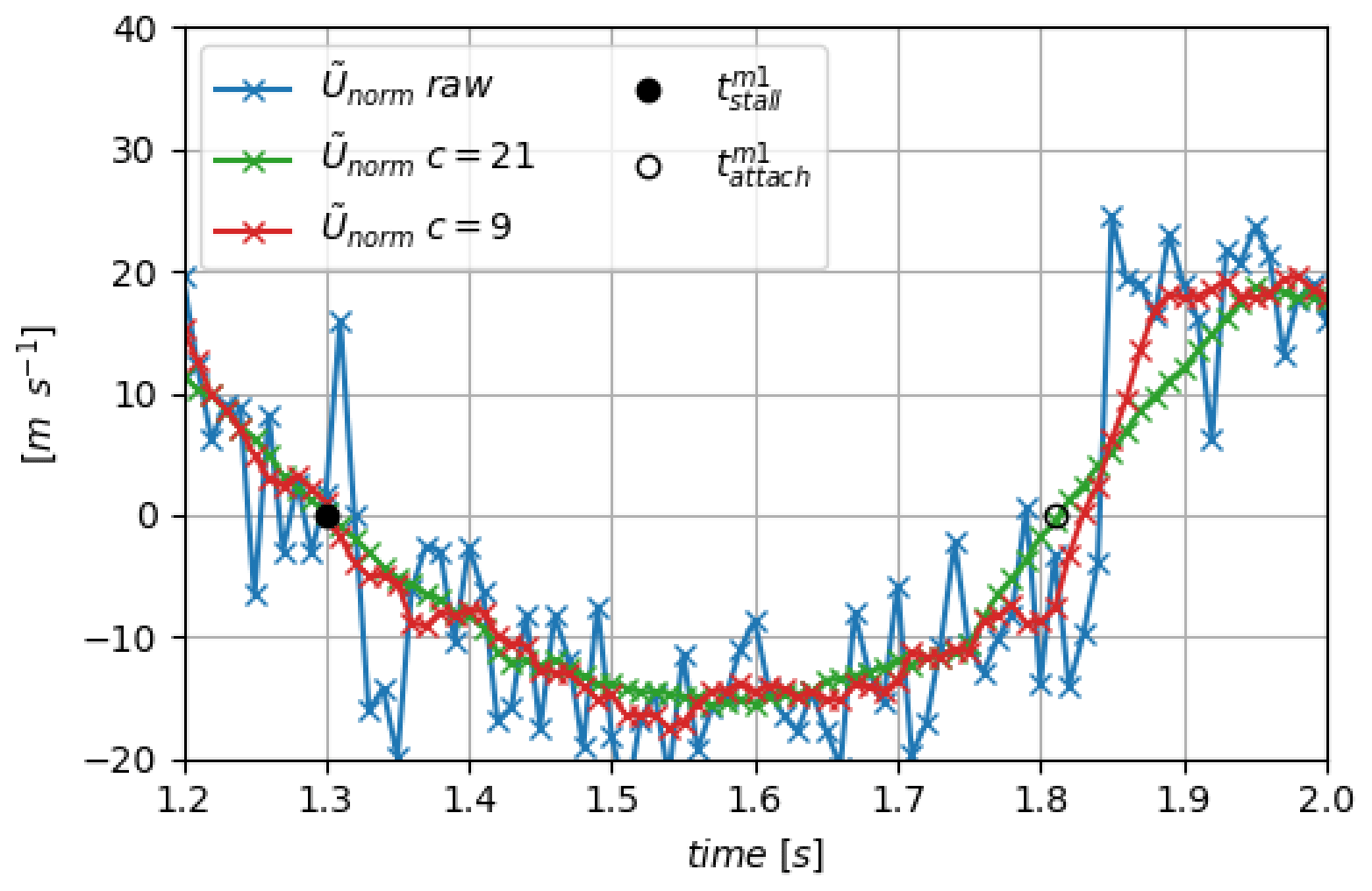
Figure 15Zoom on a period of the instantaneous signal of (variations in Unorm(t) from method (1)) and raw signal super-imposed with moving-averaged treatments with different filter width: c=9 and c=21
Then, a zero-crossing criterion is applied to extract the detected instants and . This criterion uses the Unorm(t) signal minus its mean value, , calculated over the 18 cycles so that sudden variations in the signal are located where the fluctuating signal crosses the x axis. Finally, the sign of the time derivative, , is used to discriminate stall instants from reattachment instants, and (see Fig. 16a). This zero-crossing method will also be used for detection methods 2 and 3 that follow.
The resulting detected instants and are compared to the reference instants extracted from the visualization of the instantaneous velocity fields of Sect. 4.1, and (see Fig. 16b). The first observation is that the stall and reattachment instants are detected earlier on average than the visual reference, and , respectively (or 2.5 to 4 time steps), which is to be related to the smoothing procedure used. Then, a certain dispersion exists in the detected instants that can be quantified using the standard deviations and . Knowing the time resolution is , the same order of magnitude is found for the reference from visualization and for the velocity field, and . The higher dispersion in the reattachment process is at the limit of the measurement precision. However, this trend is observed in the phased averaged signal (sharper peak of time derivative) from visualization of the flow (larger width of the hatched areas) and will also be shown later with methods 2 and 3 (see Table 1).
4.2.2 Method 2
Another flow separation detection method is introduced with, this time, a criterion associated with instantaneous vortices from shear layers. Indeed, the vertical distance between identified vortices in the separated shear layers forming the blade wake width is used, directly related to the flow separation location on the aerodynamic surface (Yarusevych et al., 2009) (see Sect. 3.2 on the vortex identification method). The wake width is defined as
with subscripts clock and counterclock corresponding to quantities from the clockwise and counterclockwise rotating vortices, respectively, and N the number of vortices identified at the time t. The obtained signal can be phase averaged, , as presented in Fig. 17a. Time derivative peaks of the signal are close to the reference instants, for which standard deviation is represented by green and red hatched areas. This constitutes a first validation of the method.
As in the first method, the zero-crossing criterion is applied to the resulting smoothed signal W(t) to obtain stall and reattachment instants for each instantaneous oscillating cycle, and . The first results show that the mean detected stall instant is closer to the visual reference, i.e. (less than one time step), than the first detection method presented in Sect. 4.2.1. However, this is accompanied by a high value of the standard deviation, , way larger than with other methods (see Table 1). This augmentation is to be related to the difficulty to detect the small vortices when shear layers are close to the blade surface and because their size is of the order of magnitude of the spatial resolution of PIV measurements. For the detection of reattachment instants, the method is more reliable as shear layer vortices are bigger and further away from the surface. However, the reattachment instants are detected significantly earlier on average than the visual reference (about five time steps: Fig. 17b), due to the smoothing procedure and similarly to method 1.

Figure 16Results from the zero-crossing method applied to the (variations in Unorm(t)): (a) instantaneous signals with detected instants; (b) normalized delay of the stall and reattachment detected instants.
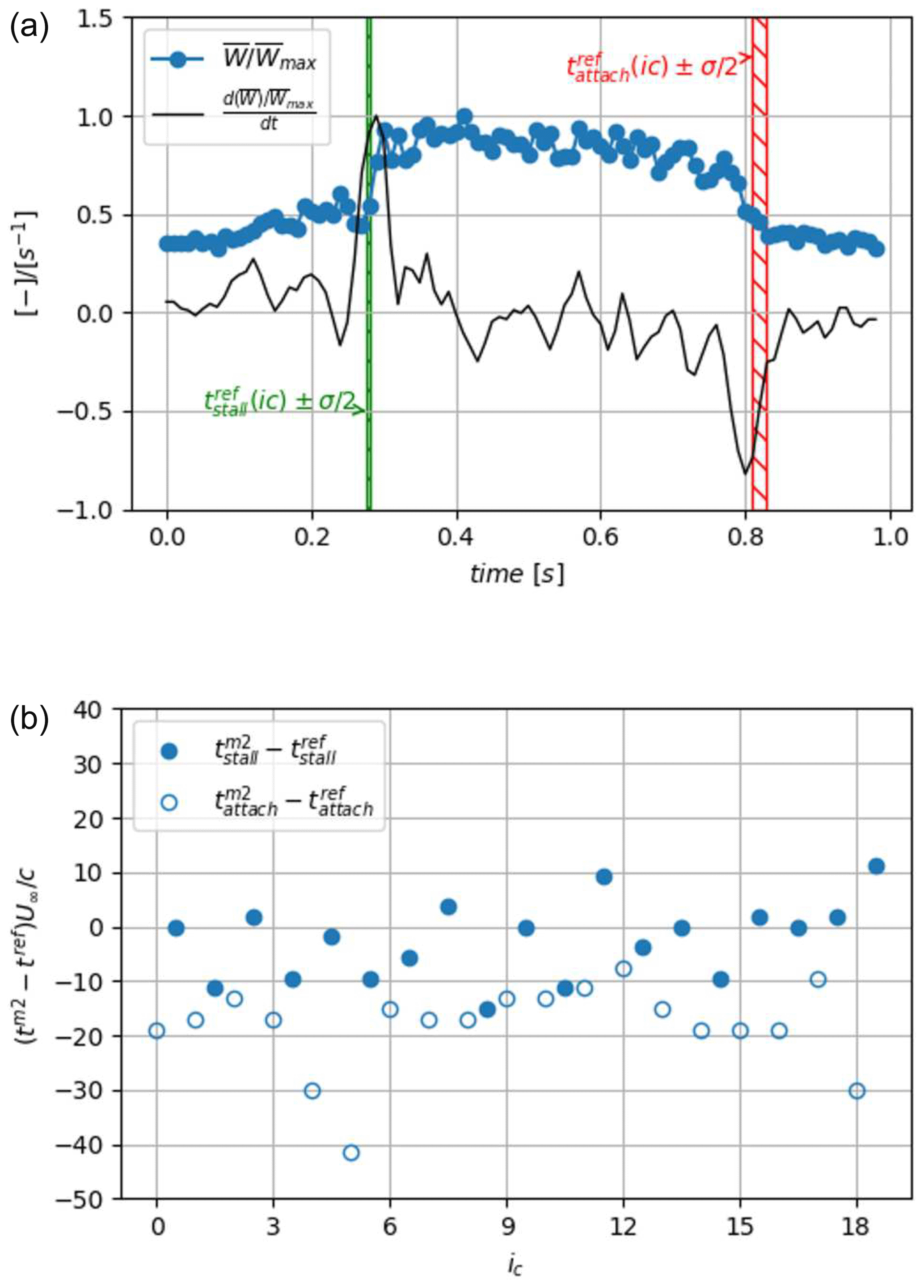
Figure 17Second method to detect the flow stall–reattachment instants. (a) The phase average signal with its time derivative ; (b) results of the zero-crossing method to extract the flow stall–reattachment instants using the second method, and , compared to reference instants. The time window width marked by green and red hatched areas corresponds to the standard deviation centered on the average of the reference instants extracted from the instantaneous velocity fields of Sect. 4.1, or . The filled circle symbols correspond to stall instants, and void circle symbols correspond to reattachment instants.
4.2.3 Method 3
These two previous methods provide an instantaneous detection of the flow stall–reattachment phenomena. To further explore the detection of these instants, we choose to use another method based on statistics introduced in Sect. 3.3. It was already used in the context of wind energy and helicopter blades for the analysis of the dynamic stall phenomenon by Melius et al. (2016) and Mulleners and Raffel (2012). The chosen vector field for the present analysis focuses on the separated shear layer dynamics rather than the wake dynamics from the initial PIV field of view (see Fig. 18). A total of 2000 snapshots were used with no distinction of the phase, which enables the extraction of the flow separation state within the first POD modes as explained by Melius et al. (2016) and Mulleners and Raffel (2012). As a first approach, the phase average of the two first POD modes is presented in Fig. 19 with temporal coefficients a1(t) and a2(t). The first mode of the eigenvector field presented in Fig. 19a (i.e. ) contains 77 % of the total turbulent kinetic energy (i.e. Λ1∼0.77) and captures accelerations and deceleration of the flow over the profile depending on the sign of the associated temporal coefficient a1(t). The transitions between the acceleration (i.e. a1(t)<0) and deceleration (i.e. a1(t)>0) phases are marked by abrupt variations in amplitude, which should be associated with instants of the stall and reattachment phenomena. The second mode of the eigenvector field presented in Fig. 19b (i.e. ) contains much less turbulent kinetic energy (i.e. Λ2∼0.049) and exhibits a shear layer with a shear direction that changes accordingly with the sign of its associated temporal coefficient a2(t). This variation in shear may be associated with the passage of the leading edge vortex associated with dynamic stall (dynamic stall vortex) created during unsteady variations in the angle of incidence as pointed out by Melius et al. (2016) and Mulleners and Raffel (2012). Interestingly, a minimum of a2(t) occurs significantly ahead of the flow stall–reattachment instants contrary to the first mode. However, studying the ability of the e-TellTale sensor to detect dynamic stall vortex needs further experimental investigations that will not be performed in this work. The following will therefore focus on the first POD mode.
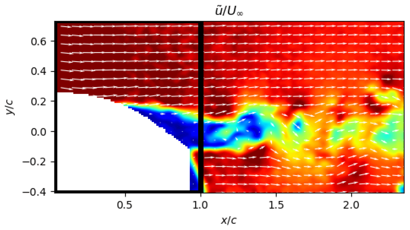
Figure 18Reduced field of view (black rectangle) used for the third detection method using POD.
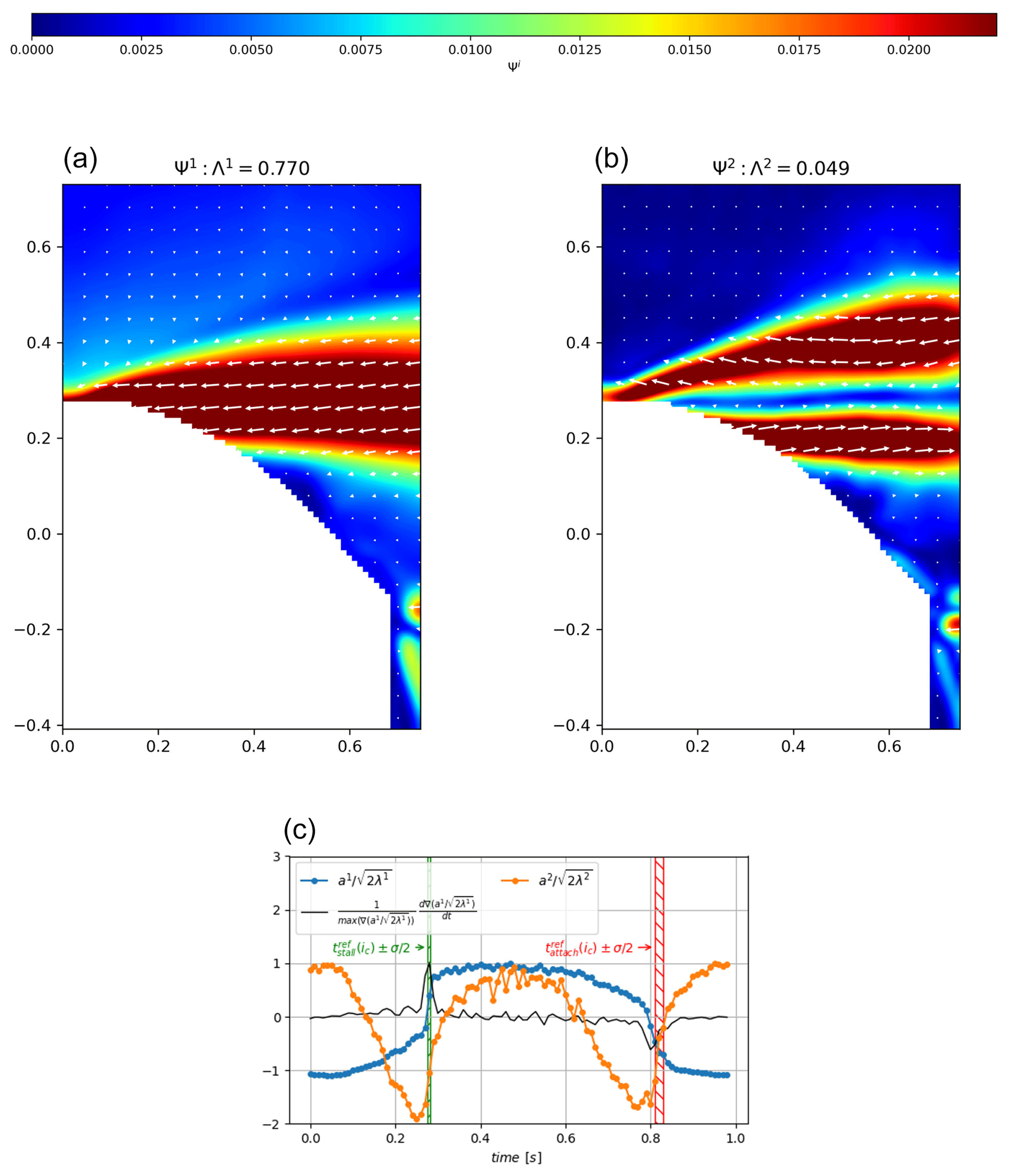
Figure 19Third method to detect the flow stall–reattachment instants: (a) and (b) are isocontours of the eigenvector field , of the nth mode, with isocontours of its modulus superimposed. Λn is the eigenvalue of the nth mode, representing the part of the turbulent kinetic energy in the mode. Panel (c) represents the phase average of the corresponding temporal coefficients scaled with their turbulent kinetic energy content () . The time window width marked by green and red hatched areas corresponds to the standard deviation centered on the average of the reference instants extracted from the instantaneous velocity fields of Sect. 4.1, or
The coefficient of the first mode a1(t) was also studied instantaneously to compare with the other detection methods. A zero-crossing criterion was applied to this instantaneous signal, leading to detected stall and reattachment instants and . The first results show that these instants follow the trend of the first detection method regarding the mean quantities, i.e., the detection occurs earlier than the visual reference similar to methods 1 and 2: and , and the dispersion is also similar to the visual reference, i.e., and . The delay is to be attributed to the smoothing procedure while the trend regarding the higher dispersion on the reattachment process is retrieved.
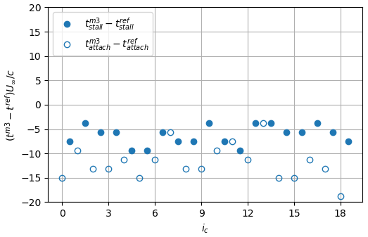
Figure 20Results of the zero-crossing method to extract the flow stall–reattachment instants using the third method. The filled circle symbols correspond to stall instants, , and void circle symbols correspond to reattachment instants, .
4.2.4 Synthesis and comparison of detection methods
From PIV measurements there is no unique criterion to detect stall instants. Thus four known or developed methods were used to detect both the stall and reattachment phenomena. Each method uses different spatiotemporal features of the flow over an oscillating profile, from the TR-PIV measurements. As a first approach, the phase average signal is analyzed. All methods exhibit a phase average signal with the sudden variations associated with the stall and reattachment phenomena. Corresponding instants can be extracted using a computation of the time derivative, and the sign of this time derivative enables us to distinguish the stall from the reattachment phenomenon. The extracted stall and reattachment instants were found equivalent for all methods (within one to two time steps) to instants that can be extracted from the visual inspection of instantaneous vector fields, which provide a first validation of the methods. Then, targeting real-time monitoring and/or real-time control, the signals extracted from all methods were explored instantaneously. Methods 1 and 3 were found to detect the stall and reattachment phenomena similarly with an earlier (from 2.5 to 4 time steps) detection of the reattachment phenomenon compared to visual inspection of instantaneous vector fields. This early detection is to be attributed to the bias of the smoothing procedure on the slopes. Method 2 has a stall detection that occurs at similar values to those that can be observed (visual reference) but with a larger standard deviation. This particularity is found to be related to the difficulties in detecting vortices close to the blade surface. At last, all methods exhibits a larger duration and dispersion of the detected instants for the reattachment process, which is here highlighted as a particularity of this process.
4.3 Ability of the e-TellTale sensor to detect flow stall
Detection methods using TR-PIV measurements will be compared to the detection method using the e-TellTale sensor. For that purpose, the phase-averaged strip position, , is detected from image processing as explained in Sect. 3.1 and presented in Fig. 21 together with the time-averaged standard deviation of stall and reattachment instants detected from the instantaneous flow field (i.e., green and red hatched areas, respectively). It is observed that the position of the strip during the oscillation cycle is characterized by two sudden changes, revealed with the time derivative peaks, in very good agreement with the stall and reattachment instants observed with the instantaneous flow field. This is a first validation of the e-TellTale sensor to detect stall and reattachment instants.
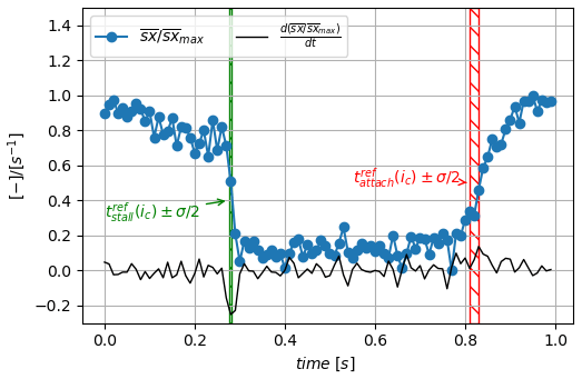
Figure 21The evolution of dimensionless phase-averaged streamwise coordinate of the center of the strip, , during the oscillation cycle (blue dotted line) together with its time derivative (black line). The time window width marked by the red hatched area corresponds to the standard deviation centered on the averaged . The time window width marked by the green hatched area corresponds to the standard deviation value centered on the phase-averaged .
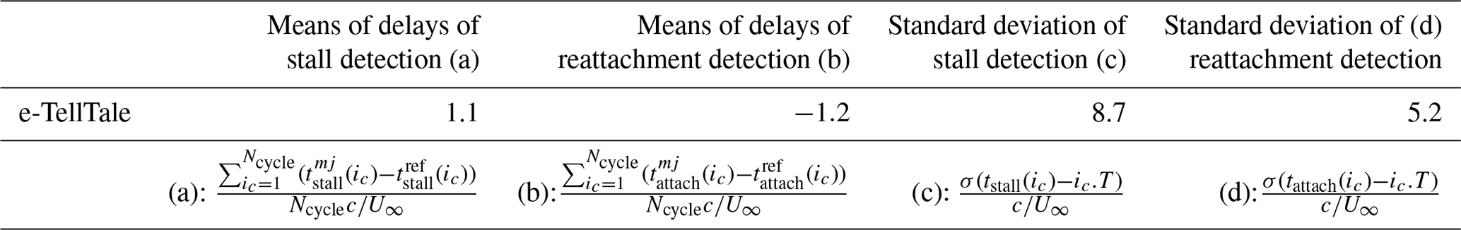
To further characterize the detected instants from the movement of the strip, the zero-crossing criterion is applied to the corrected instantaneous signal of the position of the strip, sxc(t). Resulting stall and reattachment instants subtracted from the reference instants, and , are plotted in Fig. 22 and summarized in Table 2. Contrary to what was found from other methods, the mean value is very close to the visual reference (i.e., close to zero). As can be seen in Fig. 23, this is related to the fact that the strong slope is now centered around zero, due to the bias introduced with the correction applied to the original signal sx(t) (Fig. 5). The smoothing procedure has thus no effect on the detected instants. A particularity of the e-TellTale sensor, which remains an open question, is related to the standard deviation of the stall and reattachment process, respectively and , which is more important for the stall than for the reattachment phenomenon. One hypothesis is that fluctuations of the e-TellTale strip movements are more sensitive to fluctuations of turbulent structures in the stalled configuration because they are larger and further away from the wall. This however needs further investigations at a higher acquisition rate.
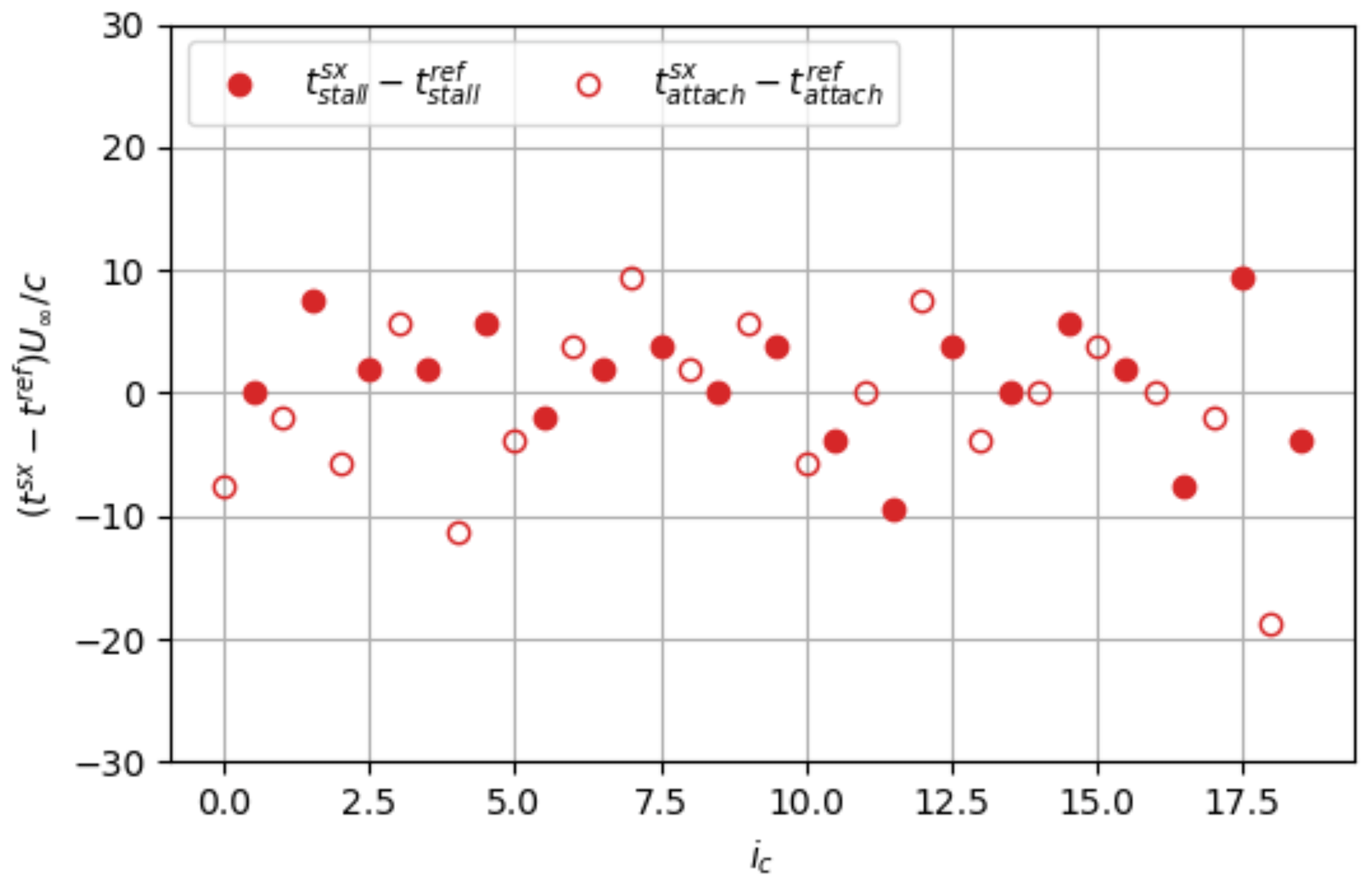
Figure 22Results of the zero-crossing method to extract the flow stall–reattachment instants using the strip position. The filled circle symbols correspond to stall instants, , and void circle symbols correspond to reattachment instants, .

Figure 23Zoom on a period of the corrected signal (variations in sxc(t)) with the detected instants and the smoothed signal superimposed using two filter sizes c=9 and c=21.
Table 2Summary of stall–reattachment detected instants, the three methods and the e-TellTale sensors. All times are expressed as chord times .
The ability of an original e-TellTale sensor to detect flow stall–reattachment instants during oscillations of the angle of incidence of a blade section has been explored. For that purpose, a 2D NACA 654-421 blade section equipped with an e-TellTale sensor in the aft region has been set in the LHEEA aerodynamic wind tunnel. The blade was oscillating around the stall angle to reproduce a constant shear inflow perturbation in front of a rotating wind turbine blade at a chord Reynolds number of 2.105. Three methods to detect the flow stall–reattachment instants have been successfully applied using time-resolved-PIV measurements during the blade oscillation cycle. This includes two instantaneous methods: the direct use of the tangential instantaneous velocity (method 1) and the instantaneous extraction of shear layer vortices (method 2). One statistical method is also tested using POD (method 3). Also, two types of treatments were applied to the extracted signal from the different methods: a phase-averaged treatment on the blade oscillating cycle and a direct use of the instantaneous signal.
The phase-averaged signals of all methods give similar results of the detected stall and reattachment instants within accuracy of one to two time steps. Moreover, the sign of the time derivative can be used to easily discriminate the stall from the reattachment process.
The direct use of the instantaneous signals needs prior smoothing before applying the zero-crossing method to extract stall and reattachment instants. Methods 1 and 3 were found equivalent, with an earlier detection of the stall and the reattachment instants (2.5 to 4 time steps earlier), to be attributed to the smoothing method. Method 2, using an instantaneous detection of vortices, is not able to have an accurate detection of the stall instants due to the limitation of the spatial resolution close to the wall. However, reattachment instants were detected similarly to other methods. Also, all the detection methods present a more sudden and less disperse stall phenomenon than the reattachment process.
Then, results of these methods were compared to movement of the e-TellTale strip. The phase-averaged signal of the strip movement is well correlated with all methods. This constitutes a first validation of the e-TellTale strip capabilities to follow the stall–reattachment dynamics. Also, when removing the smoothing effect, similar results were found regarding the mean values of the detected instants from an instantaneous processing of the strip position signal, which constitute another validation of the ability of the e-TellTale strip to follow the stall–reattachment dynamics. An open question remains regarding fluctuations of the strip motion which do not follow the trend found by other methods: higher fluctuations of the detected instants for the reattachment process than for stall process. Further investigations are needed with a higher acquisition rate to investigate these higher-order fluctuations of the strip position. In addition to the demonstration of the e-TellTale ability to detect stall–reattachment instants, this paper introduces a methodology that could be used to evaluate the ability to extract other flow features of the blade aerodynamics such as the well-known dynamic stall vortex or the blade wake dynamics. Also, what remains to be found is a link between this dynamic strip position and the dynamic response of the e-TellTale strain gauge signal.
Data can be made available upon request.
Experiments were conceived and planned by CB, AS and DV. AS carried out experiments under the supervision of CB. AS carried out the PIV post-processing. AS implemented the post-processing and detection methods (except the POD method) under the supervision of CB. AS implemented the POD method in collaboration with BP and under the supervision of CB. Analyses were performed by AS under the supervision of CB, except for the POD detection methods, which were discussed together with AS, CB and BP. AS wrote the first draft of the manuscript; reviews of the manuscript were performed by CB. A review of the manuscript regarding the POD part was performed by BP. AS's PhD grant was obtained by DV. Other costs related to experiments were shared between CB's and DV's own funding.
The authors declare that they have no conflict of interest.
This article is part of the special issue “Wind Energy Science Conference 2019”. It is a result of the Wind Energy Science Conference 2019, Cork, Ireland, 17–20 June 2019.
The authors would like to thank Jean-Jacques Lasserre and Philippe Galtier for the PIV Dantec equipment loan and their assistance during measurements. We also would like to thank Vincent Jaunet for his help during the PIV acquisition. This work was partly carried out within the framework of the WEAMEC, West Atlantic Marine Energy Community, and with funding from the city of Nantes, the Pays de la Loire Region and Centrale Nantes in France.
This research has been supported by WEAMEC – West Atlantic Marine Energy Community (grant no. 2018 ASAPe) and by the French agency ADEME (grant no. 1682C0155 EPENON).
This paper was edited by Gerard J. W. van Bussel and reviewed by two anonymous referees.
Aubrun, S., Garcia, E. T., Boquet, M., Coupiac, O., and Girard, N.: Wind turbine wake tracking and its correlations with wind turbine monitoring sensors. Preliminary results, J. Phys., 753, 032003, https://doi.org/10.1088/1742-6596/753/3/032003, 2016. a
Batlle, E. C., Pereira, R., and Kotsonis, M.: Airfoil Stall Hysteresis Control with DBD Plasma actuation, 55th AIAA Aerospace Sciences Meeting, Grapevine, Texas, 9–13 January 2017, 1–8, No. 19803, https://doi.org/10.2514/6.2017-1803, 2017. a
Bossanyi, E. A., Kumar, A., and Hugues-Salas, O.: Wind turbine control applications of turbine-mounted LIDAR, J. Phys., 555, 012011, https://doi.org/10.1088/1742-6596/555/1/012011, 2014. a
Braud, C. and Liberzon, A.: Real-time processing methods to characterize streamwise vortices, J. Wind Eng. Ind. Aerod., 179, 14–25, https://doi.org/10.1016/j.jweia.2018.05.006, 2018. a
Cahuzac, A., Boudet, J., Borgnat, P., and Lévêque, E.: Smoothing algorithms for mean-flow extraction in large-eddy simulation of complex turbulent flows, Phys. Fluids, 22, 125104, https://doi.org/10.1063/1.3490063, 2010. a
Chamorro, L. P., Guala, M., Arndt, R. E. A., and Sotiropoulos, F.: On the evolution of turbulent scales in the wake of a wind turbine model, J. Turbul., 27, 13, https://doi.org/10.1080/14685248.2012.697169, 2012. a
Choudhry, A., Leknys, R., Arjomandi, M., and Kelso, R.: An insight into the dynamic stall lift characteristics, Exp. Therm. Fluid Sci., 58, 188–208, https://doi.org/10.1016/j.expthermflusci.2014.07.006, 2014. a
Corten, G. P.: Flow separation on wind turbines blades, PhD thesis, University Utrecht, Utrecht, the Netherlands, 2001. a
De Gregorio, F., Albano, F., and Lupo, M.: Flow separation investigation by PIV technique, in: 7th International Symposium on Particle Image Velocimetry, Rome, Italy, 11–14 September 2007 , 2007. a
Devinant, P., Laverne, T., and Hureau, J.: Experimental study of wind-turbine airfoil aerodynamics in high turbulence, J. Wind Eng. Ind. Aerod., 90, 689–707, 2002. a
Emeis, S.: Wind Energy Meteorology: Atmospheric Physics for Wind Power Generation, Springer, Berlin, Germany, 2018. a
Garcia, D.: A fast all-in-one method for automated post-processing of PIV data, Exp. Fluids, 50, 1247–1259, https://doi.org/10.1007/s00348-010-0985-y, 2011. a
Holmes, P., Lumley, J. L., and Berkooz, G.: Turbulence, Coherent Structures, Dynamical Systems and Symmetry, Cambridge University Press, Cambridge, UK, https://doi.org/10.1017/CBO9780511622700, 1996. a
Jaunet, V. and Braud, C.: Experiments on lift dynamics and feedback control of a wind turbine blade section, Renew. Energ., 126, 65–78, https://doi.org/10.1016/j.renene.2018.03.017, 2018. a, b, c
Jeong, J. and Hussain, F.: On the identification of a vortex, J. Fluid Mech., 285, 69–94, https://doi.org/10.1017/S0022112095000462, 1995. a
Jones, R. T.: The unsteady lift of a wing of finite aspect ratio, Technical Report NASA-R681, NASA Langley, US, 13 pp., 1940. a
Melius, M., Cal, R. B., and Mulleners, K.: Dynamic stall of an experimental wind turbine blade, Phys. Fluids, 28, 034103, https://doi.org/10.1063/1.4942001, 2016. a, b, c
Michard, M., Graftieaux, L., Lollini, L., and Grosjean, N.: Identification of vortical structures by a non local criterion – Application to PIV measurements and DNS-LES results of turbulent rotating flows, in: 11th Symposium on Turbulent Shear Flows, Grenoble, France, 8–11 September 1997, 28–25, 1997. a
Mulleners, K. and Raffel, M.: The onset of dynamic stall revisited, Exp. Fluids, 52, 779–793, https://doi.org/10.1007/s00348-011-1118-y, 2012. a, b, c
Mulleners, K. and Raffel, M.: Dynamic stall development, Exp. Fluids, 54, 1469, https://doi.org/10.1007/s00348-013-1469-7, 2013. a
Norberg, C.: Fluctuating lift on a circular cylinder: review and new measurements, J. Fluid. Struct., 17, 57–96, https://doi.org/10.1016/S0889-9746(02)00099-3, 2003. a
Pechlivanoglou, G.: Passive and active flow control solutions for wind turbine blades, PhD thesis, Technical University of Berlin, Berlin, Germany, available at: https://depositonce.tu-berlin.de/handle/11303/3784 (last access: 22 February 2021), 214 pp., 2013. a
Pedersen, M. M., Larsen, T. J., Madsen, H. Aa., and Larsen, G. Chr.: Using wind speed from a blade-mounted flow sensor for power and load assessment on modern wind turbines, Wind Energ. Sci., 2, 547–567, https://doi.org/10.5194/wes-2-547-2017, 2017. a
Pedersen, T. F., Sørensen, N. N., and Enevoldsen, P.: Aerodynamics and Characteristics of a Spinner Anemometer, J. Phys., 75, 012018, https://doi.org/10.1088/1742-6596/75/1/012018, 2007. a
Rezaeiha, A., Pereira, R., and Kotsonis, M.: Fluctuations of angle of attack and lift coefficient and the resultant fatigue loads for a large Horizontal Axis Wind turbine, Renew. Energ., 114, 904–916, https://doi.org/10.1016/j.renene.2017.07.101, 2017. a
Sirovich, L.: Turbulence and the dynamics of coherent structures. I – Coherent structures. II, Q. Appl. Math., 45, 561–571, https://www.jstor.org/stable/43637457, 1987. a
Soulier, A., Voisin, D., Danbon, F., and Braud, C.: Electronic TellTale (E - penon) sensor to detect flow separation on wind-turbines blades, in: Wind Energy Science Conference, Copenhagen, Denmark, 26–29 June 2017, p. 276, 2017. a, b
Swytink-Binnema, N. and Johnson, D. A.: Digital tuft analysis of stall on operational wind turbines: Digital tuft analysis of stall on operational wind turbines, Wind Energy, 19, 703–715, https://doi.org/10.1002/we.1860, 2016. a
Troldborg, N., Bak, C., Madsen, H. A., and Skrzypinski, W. R.: DANAERO MW: Final Report, Technical Report, DTU Wind Energy, Denmark Roskilde, 143 pp., 2013. a
Yarusevych, S., Sullivan, P. E., and Kawall, J. G.: On vortex shedding from an airfoil in low-Reynolds-number flows, J. Fluid Mech., 632, 245–271, https://doi.org/10.1017/S0022112009007058, 2009. a, b, c, d