Wind turbines in atmospheric flow: fluid–structure interaction simulations with hybrid turbulence modeling

In order to design future large wind turbines, knowledge is needed about the impact of aero-elasticity on the rotor loads and performance and about the physics of the atmospheric flow surrounding the turbines. The objective of the present work is to study both effects by means of high-fidelity rotor-resolved numerical simulations. In particular, unsteady computational fluid dynamics (CFD) simulations of a 2.3 MW wind turbine are conducted, this rotor being the largest design with relevant experimental data available to the authors. Turbulence is modeled with two different approaches. On one hand, a model using the well-established technique of improved delayed detached eddy simulation (IDDES) is employed. An additional set of simulations relies on a novel hybrid turbulence model, developed within the framework of the present work. It consists of a blend of a large-eddy simulation (LES) model by Deardorff for atmospheric flow and an IDDES model for the separated flow near the rotor geometry.

In the same way, the assessment of the influence of the blade flexibility is performed by comparing two different sets of computations. The first group accounts for a structural multi-body dynamics (MBD) model of the blades. The MBD solver was coupled to the CFD solver during run time with a staggered fluid–structure interaction (FSI) scheme. The second set of simulations uses the original rotor geometry, without accounting for any structural deflection. The results of the present work show no significant difference between the IDDES and the hybrid turbulence model. In a similar manner, and due to the fact that the considered rotor was relatively stiff, the loading variation introduced by the blade flexibility was found to be negligible when compared to the influence of inflow turbulence. The simulation method validated here is considered highly relevant for future turbine designs, where the impact of blade elasticity will be significant and the detailed structure of the atmospheric inflow will be important.

1 Introduction

As future wind turbines will have unprecedentedly long and flexible blades, the necessity of understanding the effects of aero-elasticity on the rotor performance and on its structural integrity increases. Along with this, large wind turbines interact with a larger part of the atmospheric boundary layer (ABL), often exceeding the height of the atmospheric surface layer. This also needs consideration in the design phase, as the rotor blades consequently experience a large variation of flow through each revolution, and flow cases which were not relevant to consider for past designs might occur. This needed knowledge can be obtained through high-fidelity methods, such as fluid–structure interaction (FSI) simulations, which model the coupled effects of both flow and structure. These simulations can further be used to develop and improve lower-fidelity engineering models used by wind turbine designers in industry.

FSI of wind turbines in atmospheric turbulent flow is not a widely studied topic, due to the computational costs of such simulations, especially when geometrically resolved wind turbines are modeled. Instead, a more efficient approach often chosen is the use of actuator lines/discs (Sørensen and Shen, 2002; Sørensen et al., 2015). Here, the rotor is represented through body forces smeared in the computational fluid dynamics (CFD) grid, reducing the need of grid refinement significantly. An example of actuator-line-based FSI in turbulent flow is the work by Lee et al. (2013), where simulations of two aligned 5 MW wind turbines in a turbulent inflow modeled by large-eddy simulations (LES) were conducted. The structural response of the turbines was found through the FAST aero-elastic code (Jonkman and Buhl, 2005) to study the fatigue loading. It was found that especially the surface roughness and the rotor shadow effect had a large influence on the fatigue loading. As actuator lines merely represent the turbines through smeared forces, blade surface boundary layers and resultingly generated wake turbulence are not modeled. Likewise, the resulting shedding of vortices at the tips and roots is not highly resolved and improperly modeled. The far wake response is, however, sufficiently accurate when the inflow to the turbine has a high turbulence intensity (TI) (Troldborg et al., 2015).

Looking at rotor-resolved CFD/FSI, using LES is still too computationally expensive for many practical applications. Instead, compromises are needed for the turbulence models. In the works by Santo et al., FSI for wind turbines, structurally represented through finite-element shells, were studied for steady ABL flows (Santo et al., 2020a, b) using unsteady Reynolds-averaged Navier–Stokes (URANS), with the k–ϵ model. In Santo et al. (2020a), the effects of wind shear, yaw error, tilt, and tower shadow were all investigated, and it was found for instance that the introduction of yaw led to a decrease in blade deflection but a large increase in yaw moment on the hub. In Santo et al. (2020b), wind gusts were introduced by acceleration of the flow near the rotor top position. One conclusion found was that, for the setup and turbulence model used, a flow separation occurred when the velocity rapidly increased due to the gust, limiting the load increase avoiding any extreme deflections. To consider turbulent fluctuating flow, a popular alternative to LES is synthetic turbulence generators such as the method by Mann (1998). These methods efficiently create boxes of turbulent fluctuations, which can be used to create inflow for CFD simulations or inserted internally in the domain by additional body forces (Troldborg et al., 2014). Along with this, a hybrid turbulence model like detached eddy simulation (DES) can be used to resolve the turbulence in the grid. This model combines the URANS approach for attached flow regions with LES in the separated regions. The use of synthetic turbulence is efficient as the modeling of turbulent fluctuations is fast, and the DES models need less grid resolution near the rotor than LES. The turbulence will, however, not be in balance with the CFD simulation shear as shown in Troldborg et al. (2014), and therefore the turbulence will change as it convects through the domain. Another drawback of this method is that the modeled turbulence is neutrally stratified and therefore cannot naturally handle atmospheric stability. Further, a potential problem of the synthetic turbulence methods is the assumption of homogeneous and Gaussian turbulence. Even though previous work (Berg et al., 2016) has shown that the latter assumption does not significantly affect the loads on a wind turbine under normal conditions, one could easily come across cases where these assumptions do not hold. In Li et al. (2015) synthetic turbulence was used to study the geometrically resolved NREL 5 MW reference turbine in sheared and turbulent inflow including flexibility of the rotor. The FSI framework was based on a CFD solver coupled with a multi-body dynamics (MBD) structural solver, and turbulence was imposed at the inlet using the Mann turbulence box as input. The main conclusions of the study were that realistic atmospheric flow including shear and turbulence is important when designing large-scale wind turbines in terms of loading. Additionally, the study concluded that, for the specific turbine and flow cases, inclusion of blade flexibility does not highly impact the wake behavior, whereas inflow turbulence has high impacts on wake diffusion. Guma et al. (2021) recently published a study looking into the aero-elastic response of the NM80 rotor, also studied in the present article, in turbulent inflow. Here, synthetic Mann box turbulence and the delayed detached eddy simulation (DDES) turbulence model were used to create and resolve turbulent structures in the wind flow. The fluctuating forces occurring on the blades were used to calculate the fatigue damage on the blades by means of the so-called damage equivalent loading (DEL). It is found that for low inflow velocities the DEL is mainly influenced by the turbulent inflow rather than the inclusion of flexibility, at least for the considered relatively stiff rotor.

An alternative more complex method for simulating geometrically resolved turbines in the ABL flow was proposed by Vijayakumar (2015). Here, a hybrid turbulence model was developed which combines spectral ABL LES simulations by Moeng (1984) with more feasible URANS-based k–ω SAS (Egorov et al., 2010) simulations close to the rotor. By this combination, a large decrease in the necessary number of grid cells is achieved, as the URANS-based turbulence models the effect of all the turbulent scales. The model was applied to a single wind turbine blade in Vijayakumar et al. (2016), however, using pure CFD without a structural coupling.

In general, considering presently available high-performance computing capabilities, compromises are needed when doing high-fidelity aero-elastic modeling of wind turbines in atmospheric flow using FSI – either by reducing the rotor representation by actuator lines to allow LES simulations or instead by simplifying the turbulence modeling.

The objective of the present study is to move one step up the ladder of complexity by investigating rotor aerodynamics and aero-elasticity in turbulent LES inflow, using a novel turbulence model. The model is inspired by the one of Vijayakumar et al. (2016), combining the ABL turbulent flow modeling of the Deardorff LES model with the improved delayed detached eddy simulation (IDDES) engineering model near the rotor. This study considers blade resolved FSI simulations of the 2.3 MW NM80 wind turbine rotor including blade flexibility using a FSI coupling framework combining the CFD code EllipSys3D (Michelsen, 1992, 1994; Sørensen, 1995) and the structural solver from the aero-elastic code HAWC2 (Larsen and Hansen, 2007). For the specific rotor, measurements of inflow and blade loading are available for comparison with the computed results. The study is a continuation of Grinderslev et al. (2021), where FSI of the NM80 rotor was studied in various flow scenarios with sheared and yawed, albeit laminar, inflow using URANS turbulence modeling. The flow scenario studied here resembles one of these studied laminar scenarios, albeit with turbulent inflow through the novel hybrid turbulence model and an adjusted grid setup.

2 Methodology

In this section, the computational solvers are presented along with the simulation strategies such as FSI framework and precursor simulations. Further, the participating turbulence models will be introduced, to prepare for the discussion of the hybrid model. Finally, the computational grids used in the study are described along with the chosen simulation parameters.

2.1 Numerical methods

2.1.1 Flow solver

To solve the fluid flow, the DTU in-house CFD code EllipSys3D (Michelsen, 1992, 1994; Sørensen, 1995) is used. The code solves the incompressible Navier–Stokes equations in structured curvilinear coordinates using the finite-volume method with a collocated grid arrangement. The code is parallel and highly scalable using the message passing interface (MPI) and multi-block decomposition, the multi-grid method and grid sequencing. EllipSys3D has multiple convective schemes implemented, such as central difference (CDS), second-order upwind (SUDS), and quadratic upstream interpolation for convective kinematics (QUICK). For the solution of the pressure correction equation, various algorithms are implemented such as PISO, SIMPLE, SIMPLEC, and variations thereof. The Rhie–Chow interpolation is used to avoid odd–even pressure decoupling. Overset capabilities, including grid hole cutting, are implemented internally in the code (Zahle et al., 2009).

Several turbulence models are implemented such as two-equation Reynolds-averaged Navier–Stokes (RANS) models, k–ϵ and k–ω among others; hybrid models like DES, DDES, and IDDES; and multiple LES models. In addition to these, a hybrid version of the LES and the IDDES model will be presented in this paper.

For FSI simulations, the deformation of grids is handled through a moving mesh method with a blend factor. The surface displacement is propagated along the grid lines normal to the surface, with a blend factor gradually diminishing to zero with increasing distance to the blade surface. The blending can be either linear in the distance to the blade surface or based on a tanh function. This ensures that mesh points in the vicinity of the blade surface are displaced as a solid body movement along with the blade, while points further away only move a fraction of the displacement. When using the overset grid method, the deformation is only transferred to the volume grid blocks containing the solid surface.

The code has been used extensively for a range of test cases and was validated in, e.g., the Mexico project (Bechmann et al., 2011; Sørensen et al., 2016) and for the Phase VI NREL rotor (Sørensen and Schreck, 2014; Sørensen et al., 2002). Recently, the code was validated in Grinderslev et al. (2020b) for the specific case of the present NM80 rotor in atmospheric laminar flow conditions by comparison with the CFD code Nalu-Wind (Sprague et al., 2019) and measurements from the DanAero experiments. Further, the FSI framework was used in Grinderslev et al. (2021) to simulate the coupled effects of the DanAero-inspired laminar wind flow and the structural response.

2.1.2 Aero-elastic solver

HAWC2 (Larsen and Hansen, 2007) is an aero-elastic code developed at DTU used for calculating blade element momentum (BEM) aerodynamics and structural responses of wind turbines. The structural part of the code is based on the multi-body dynamics formulation, accounting for non-linear effects of large deflections. Each structural component – i.e., a blade or the tower – can be represented by a number of bodies assembled by linear Euler or Timoshenko beam elements. Sub-bodies are connected with constraint equations considering non-linearities.

HAWC2 has a built-in aerodynamics module that calculates aerodynamic forces using BEM theory. As is common in BEM implementations, prediction of airfoil aerodynamic performance is based on pre-computed look-up tables of lift, drag, and moment, which are needed to calculate forces along the blade. Multiple correction schemes are implemented to improve the BEM aerodynamics, such as tip loss corrections, dynamic stall models, tower shadow effect, and many more; see Madsen et al. (2020).

HAWC2 is widely used by industry, and it has been verified and validated in Pavese et al. (2015) and Madsen et al. (2020), considering the structural and aerodynamics aspects of the code, respectively.

2.1.3 FSI framework

The codes EllipSys3D and HAWC2 are coupled, in a partitioned manner, through the Python framework, referred to as the DTU coupling, originally created by Heinz et al. (2016a) and further developed by Horcas et al. (2019) and García Ramos et al. (2021). Through the use of the coupling framework, the BEM aerodynamics module of HAWC2 is replaced by an interface to the EllipSys3D CFD code.

Using predicted displacements of nodes from HAWC2, the CFD mesh is deformed, and a new flow field is found through EllipSys3D. The loads predicted by the CFD solver are then applied to the HAWC2 structural model and a new deformation is found. All communication between EllipSys3D and HAWC2 happens through the DTU coupling framework. In Heinz et al. (2016a), a loosely coupled approach was found to be sufficient for wind-energy-related cases, due to the high mass ratio between the turbine structure and air, and is therefore used.

Studies involving the application of the FSI framework, for both operational and standstill configurations, include Heinz et al. (2016a, b) and Horcas et al. (2019, 2020). The framework has been validated with experiments through simulations of a pull–release test of a wind turbine blade in the large-scale test facility of DTU; see Grinderslev et al. (2020a). The process of the framework between the main iterations can be described through the following steps:

• the displacements of the present time step are predicted by HAWC2 with second-order accuracy, using kinematics from the previous time step;

• displacements are sent to EllipSys3D, and the surface mesh is deformed, while displacements are propagated into the volume mesh using a volume blend method;

• the Navier–Stokes equations are solved to calculate the flow field for the new time step through under-relaxed sub-iterations in EllipSys3D;

• forces are computed and integrated on the CFD mesh surface and sent to HAWC2;

• forces are interpolated to the aerodynamic sections of the HAWC2 model, and actual deformations are calculated;

• unless the solution has reached the total simulation time, the simulation is advanced to the next time step and the procedure is repeated.

2.2 Turbulence modeling

A hybrid turbulence model has been developed to consider the dominant turbulence scales from the atmospheric boundary layer (ABL) down to the blade boundary layer (BBL), within the same simulation. To do this, the Deardorff one-equation LES turbulence model for ABL flows (Deardorff, 1972) is blended with the IDDES turbulence model (Shur et al., 2008), which itself is a blend between URANS modeling in the BBL and LES in the separation region outside the BBL. The blending of the two models happens through the energy equation, which is solved for in both methods. In the Deardorff model, the transport equation of sub-grid-scale (SGS) energy e is solved, whereas the transport equation for total turbulent kinetic energy k is solved in the IDDES method. These energy expressions are blended through their respective terms of diffusion, convection, production, buoyancy, and dissipation using a smooth tanh blending function. By this, e of the Deardorff model coming towards the rotor is transformed into equivalent k of the IDDES, and vice versa in the wake region. In the following, the two models will be introduced, followed by a description of the blending for the hybrid model used in this study.

2.2.1 Deardorff large-eddy simulation model

In the Deardorff LES turbulence model (Deardorff, 1972, 1980), the turbulent eddy viscosity μ_t is calculated through the expression

$$\begin{array}{}\text{(1)}& {\mathit{\mu }}_{\mathrm{t}}=C_k\mathit{\rho }{l}_{\mathrm{LES}}\sqrt{e}.\end{array}$$

Here, C_k is a constant of 0.1; ρ is the air density; and l_LES is a mixing length scale, which for neutral stratification is set equal to Δ_LES, which is the grid size, here defined as ${\mathrm{\Delta }}_{\mathrm{LES}}=(\mathrm{d}x\cdot \mathrm{d}y\cdot \mathrm{d}z{)}^{\mathrm{1}/\mathrm{3}}$, with dx, dy, and dz being the grid spacing in the respective directions.

The SGS energy, e, is found by solving the following transport equation:

$$\begin{array}{}\text{(2)}& \begin{array}{rl}{\displaystyle \frac{\mathrm{D}\mathit{\rho }e}{\mathrm{D}t}}& =-{\mathit{\tau }}_{ij}{S}_{ij}+{\displaystyle \frac{g}{{\mathit{\theta }}_{\mathrm{0}}}}{\mathit{\tau }}_{\mathit{\theta }\mathrm{w},\mathrm{LES}}-C_{\mathit{ϵ}}\mathit{\rho }{\displaystyle \frac{e^{\mathrm{3}/\mathrm{2}}}{l_{\mathrm{LES}}}}\\ & +{\displaystyle \frac{\partial }{\partial x_j}}\left(\left(\mathit{\mu }+\mathrm{2}{\mathit{\mu }}_{\mathrm{t}}\right){\displaystyle \frac{\partial e}{\partial x_j}}\right),\end{array}\end{array}$$

where g, t, and μ refer to the gravity, time, and molecular viscosity, respectively. C_ϵ is equal to 0.93, and the buoyancy SGS fluxes ${\mathit{\tau }}_{\mathit{\theta }i,\mathrm{LES}}=-{\mathit{\mu }}_{\mathit{\theta }}\frac{\partial \mathit{\theta }}{\partial x_i}$, with variable temperature θ and the eddy heat diffusivity being ${\mathit{\mu }}_{\mathit{\theta }}=\left(\mathrm{1}+\frac{\mathrm{2}{l}_{\mathrm{LES}}}{{\mathrm{\Delta }}_{\mathrm{LES}}}\right){\mathit{\mu }}_{\mathrm{t}}$. θ₀ is the surface reference temperature. The SGS stress tensor τ_ij is defined as ${\mathit{\tau }}_{ij}=-\mathrm{2}{\mathit{\mu }}_{\mathrm{t}}{S}_{ij}$ using the strain rate $S_{ij}=\mathrm{1}/\mathrm{2}\left(\frac{\partial {\mathit{u}}_i}{\partial x_j}+\frac{\partial {\mathit{u}}_j}{\partial x_i}\right)$, with u being the velocity vector.

2.2.2 SST-based detached eddy simulation models

For the k–ω SST-based DES turbulence models, μ_t is found through the standard k–ω SST (Menter, 1993) approach, which is then altered in the dissipation term depending on the chosen DES model.

$$\begin{array}{}\text{(3)}& {\mathit{\mu }}_{\mathrm{t}}=\mathit{\rho }{\displaystyle \frac{a_{\mathrm{1}}k}{\max \left(a_{\mathrm{1}}\mathit{\omega },\mathrm{\Omega }{F}_{\mathrm{2}}\right)}},\mathrm{with}{a}_{\mathrm{1}}=\mathrm{0.31}\end{array}$$

Here, k is a total turbulent kinetic energy, ω the specific dissipation rate, Ω the shear-strain rate, and F₂ a limiting blending function. k and ω are found through the following two transport equations:

For k,

$$\begin{array}{}\text{(4)}& \begin{array}{rl}{\displaystyle \frac{\mathrm{D}\mathit{\rho }k}{\mathrm{D}t}}& =-{\mathit{\tau }}_{ij}{S}_{ij}+{\displaystyle \frac{g}{{\mathit{\theta }}_{\mathrm{0}}}}{\mathit{\tau }}_{\mathit{\theta }\mathrm{w},\mathrm{DES}}-\mathit{\rho }{\displaystyle \frac{k^{\mathrm{3}/\mathrm{2}}}{\stackrel{\mathrm{̃}}{l}}}\\ & +{\displaystyle \frac{\partial }{\partial x_j}}\left[\left(\mathit{\mu }+{\mathit{\mu }}_{\mathrm{t}}{\mathit{\sigma }}_k\right){\displaystyle \frac{\partial k}{\partial x_j}}\right].\end{array}\end{array}$$

For ω,

$$\begin{array}{}\text{(5)}& \begin{array}{rl}{\displaystyle \frac{\mathrm{D}\mathit{\rho }\mathit{\omega }}{\mathrm{D}t}}& ={\displaystyle \frac{\mathit{\gamma }}{{\mathit{\nu }}_{\mathrm{t}}}}{\mathit{\tau }}_{ij}{\displaystyle \frac{\partial u_i}{\partial x_j}}-\mathit{\rho }\mathit{\beta }{\mathit{\omega }}^{\mathrm{2}}+{\displaystyle \frac{\partial }{\partial x_j}}\left[\left(\mathit{\mu }+{\mathit{\mu }}_{\mathrm{t}}{\mathit{\sigma }}_{\mathit{\omega }}\right){\displaystyle \frac{\partial \mathit{\omega }}{\partial x_j}}\right]\\ & +\mathrm{2}\left(\mathrm{1}-F_{\mathrm{1}}\right)\mathit{\rho }{\mathit{\sigma }}_{\mathit{\omega }\mathrm{2}}{\displaystyle \frac{\mathrm{1}}{\mathit{\omega }}}{\displaystyle \frac{\partial k}{\partial x_i}}{\displaystyle \frac{\partial \mathit{\omega }}{\partial x_i}}.\end{array}\end{array}$$

Here F₁ is a blending function, to shift between the standard k–ω model (F₁=1) near the surface and the k–ϵ model (F₁=0) within the boundary layer and further out, while σ_k, σ_ω, β, and γ are parameters which themselves depend on F₁. Finally β^* and σ_ω2 are constants. ν_t is the kinematic turbulent viscosity ${\mathit{\nu }}_{\mathrm{t}}={\mathit{\mu }}_{\mathrm{t}}/\mathit{\rho }$. All constants and parameters as well as blending functions F₁ and F₂ can be found in the original work by Menter (Menter, 1993). In the original work by Menter, the buoyancy term is not considered. In the EllipSys3D version of the k–ω SST, however, it is considered as the second term of the right-hand side of Eq. (4), and the flux is found as ${\mathit{\tau }}_{\mathit{\theta }i,\mathrm{DES}}=-{\mathit{\mu }}_{\mathrm{t}}\frac{\partial \mathit{\theta }}{\partial x_i}$.

The length scale which appears in the k-equation serves to switch from URANS to LES mode and is defined as:

$$\begin{array}{}\text{(6)}& \stackrel{\mathrm{̃}}{l}=\min \left(l_{k-\mathit{\omega }},l_{\mathrm{DES}}\right),\end{array}$$

where $l_{k-\mathit{\omega }}=\sqrt{k}/\left({\mathit{\beta }}^{*}\mathit{\omega }\right)$ and l_DES is the length scale in the LES region. In the standard DES model (Spalart et al., 1997; Travin et al., 2004), l_DES=C_DESΔ_DES, where ${\mathrm{\Delta }}_{\mathrm{DES}}=\max (\mathrm{d}x,\mathrm{d}y,\mathrm{d}z)$ and C_DES is a F₁-dependent parameter.

DES is known to be sensitive to sudden changes of grid refinements as grid-induced separation (GIS) can be introduced. Here, the modeled turbulent viscosity will drop instantly without the additional turbulence being resolved. It is also known to have a mismatch between the URANS and LES region, if used as a wall-modeled LES model. These issues are addressed in DDES (Menter et al., 2003; Spalart et al., 2006), IDDES (Shur et al., 2008), and SIDDES (Gritskevich et al., 2012) by using more advanced expressions for the length scale $\stackrel{\mathrm{̃}}{l}$.

2.2.3 Hybrid ABL–BBL model

In order to simulate the effect of turbulence on both ABL and BBL scales, a hybrid method is suggested where the Deardorff ABL LES model is blended together with the BBL DES models to avoid the need of excessive grid resolution in the BBL otherwise needed by LES. The blending is established through a blending function F_h, which is zero in the ABL region and one in the DES region, and then defining a hybrid turbulence kinetic energy $\stackrel{\mathrm{̃}}{k}=F_{\mathrm{h}}k+(\mathrm{1}-F_{\mathrm{h}})e$. Using these definitions, the energy equations Eqs. (2) and (4) are combined to give the following transport equation for $\stackrel{\mathrm{̃}}{k}$:

$$\begin{array}{}\text{(7)}& \begin{array}{rl}{\displaystyle \frac{\mathrm{D}\mathit{\rho }\stackrel{\mathrm{̃}}{k}}{\mathrm{D}t}}& =-{\mathit{\tau }}_{ij}{S}_{ij}+{\displaystyle \frac{g}{{\mathit{\theta }}_{\mathrm{0}}}}\left(F_{\mathrm{h}}{\mathit{\tau }}_{\mathit{\theta }\mathrm{w},\mathrm{DES}}+\left(\mathrm{1}-F_{\mathrm{h}}\right){\mathit{\tau }}_{\mathit{\theta }\mathrm{w},\mathrm{LES}}\right)\\ & -\mathit{\rho }{\stackrel{\mathrm{̃}}{k}}^{\mathrm{3}/\mathrm{2}}\left({\displaystyle \frac{F_{\mathrm{h}}}{\stackrel{\mathrm{̃}}{l}}}-C_{\mathit{ϵ}}{\displaystyle \frac{\mathrm{1}-F_{\mathrm{h}}}{l_{\mathrm{LES}}}}\right)\\ & +{\displaystyle \frac{\partial }{\partial x_j}}\left[\left(\mathit{\mu }+{\mathit{\mu }}_{\mathrm{t}}\left({\mathit{\sigma }}_k{F}_{\mathrm{h}}+\mathrm{2}\left(\mathrm{1}-F_{\mathrm{h}}\right)\right)\right){\displaystyle \frac{\partial \stackrel{\mathrm{̃}}{k}}{\partial x_j}}\right].\end{array}\end{array}$$

The blending function F_h is defined as follows:

$$\begin{array}{}\text{(8)}& F_{\mathrm{h}}=\mathrm{0.5}-\mathrm{0.5}\cdot \left(\tanh \left(\left(d_{\mathrm{w}}-R\right)\cdot {\displaystyle \frac{\mathrm{2}}{{\mathit{\delta }}_{\mathrm{blend}}}}\right)\right).\end{array}$$

Here, d_w is the wall-normal distance; R is the wall distance to the location where F_h=0.5; and δ_blend is the transition distance between F_h=0.12 and F_h=0.88, where the blend is most rapid.

To allow the present method to work together with the k–ω model, an expression for ω is needed in the LES region. This expression is made through the standard k–ω turbulent viscosity expression, to ensure consistency through the blending regimes.

$$\begin{array}{}\text{(9)}& {\mathit{\mu }}_{\mathrm{t}}=C_k\mathit{\rho }{l}_{\mathrm{LES}}\sqrt{\stackrel{\mathrm{̃}}{k}}=\mathit{\rho }{\displaystyle \frac{\stackrel{\mathrm{̃}}{k}}{{\mathit{\omega }}_{\mathrm{LES}}}}\Rightarrow {\mathit{\omega }}_{\mathrm{LES}}={\displaystyle \frac{\sqrt{\stackrel{\mathrm{̃}}{k}}}{C_k{l}_{\mathrm{LES}}}}\end{array}$$

Here, it is assumed that the blending from DES to LES happens in the region where F₂=0, such that the viscosity limiter is inactive. A blended expression $\stackrel{\mathrm{̃}}{\mathit{\omega }}$ is then found for the entire domain.

$$\begin{array}{}\text{(10)}& \stackrel{\mathrm{̃}}{\mathit{\omega }}=\mathit{\omega }{F}_{\mathrm{h}}+{\mathit{\omega }}_{\mathrm{LES}}\left(\mathrm{1}-F_{\mathrm{h}}\right)\end{array}$$

This allows the calculation of the turbulent viscosity similar to Eq. (3):

$$\begin{array}{}\text{(11)}& {\mathit{\mu }}_{\mathrm{t}}=\mathit{\rho }{\displaystyle \frac{a_{\mathrm{1}}\stackrel{\mathrm{̃}}{k}}{\max \left(a_{\mathrm{1}}\stackrel{\mathrm{̃}}{\mathit{\omega }},F_{\mathrm{2}}\mathrm{\Omega }\right)}}.\end{array}$$

It is noted that in the Deardorff part of the model the turbulent viscosity, μ_t, is linearly proportional to the length scale, l_LES, through ω_LES; see Eq. (9). This needs to be considered if sudden changes are made to the grid resolution, as this will lead to a proportionally equal change to μ_t. This could for instance be the case with overset grids, as used in the present study, where sudden changes of grid resolutions are happening over the interface. This should in theory be fine, as the resolved turbulence adapts to the grid, but, as seen with the known GIS issues of the original DES model, the change in resolved turbulence, due to grid refinement, does not happen instantaneously. In the present study, this is handled by limiting the LES length scale Δ_LES to the grid size of the background grid; see Sect. 2.3.1.

2.2.4 Turbulent inflow simulations

In this study, the turbulent flow of the atmospheric boundary layer is modeled through a LES precursor simulation using the Deardorff model. Here, a neutrally stratified wind profile is simulated and sampled for use as input in the successor simulation including the rotor.

In the successor simulation the hybrid LES–IDDES model is used. LES is used for turbulence modeling in the majority of the domain, except for the region close to the rotor. In this area, the IDDES model is utilized instead, which removes the LES grid requirement near the rotor surface.

The precursor conditions are approximating measurements from the DanAero field experiment (Bak et al., 2010), where a met mast located ≈2.5 diameters from the considered rotor measured the wind field using cup anemometers at six points vertically, 17, 28.5, 41, 57 (hub height), 77, and 93 m. The data set from these cup anemometers is used to fit a corresponding neutral log-law wind profile to generate inputs for the Schumann–Grötzbach (SG) wall model (Schumann, 1975; Grötzbach, 1987) used in the simulation.

$$\begin{array}{}\text{(12)}& U=u_{*}/\mathit{\kappa }\cdot \ln \left(z/z_{\mathrm{0}}\right),\end{array}$$

where U is the wind speed, u_* the friction velocity, κ the von Kármán constant (≈0.4), z the vertical coordinate, and finally z₀ the roughness length. As a neutral stratification flow is modeled for simplicity, no temperature is modeled in the present study.

2.3 Simulation setups

2.3.1 EllipSys3D model

Air is described with a density of 1.22 kg m⁻³ and a dynamic viscosity of $\mathrm{1.769}\times {\mathrm{10}}^{-\mathrm{5}}$ kg m⁻¹ s⁻¹. The convective terms are calculated through a blend of the fourth-order central difference (CDS4) scheme in the LES area and the upwind QUICK scheme in the URANS part as described by Strelets (2001). An improved version of the SIMPLEC algorithm (Shen et al., 2003) is used to couple the velocity and pressure. No transition model is applied, such that the blade boundary layer is assumed fully turbulent. A time increment corresponding to 0.125^∘ rotation per time step is used for all simulations, corresponding to $\mathrm{1.29}\times {\mathrm{10}}^{-\mathrm{3}}$ s per time step. The rotation speed of the rotor is constant at 16.2 rpm, resulting in an effective Reynolds number of ≈6 million along the majority of the blade for the studied flow case.

Turbulence blending

To enable the hybrid turbulence modeling, a blending region must be defined. As mentioned in Sect. 2.2.3, a sudden grid refinement will create a sudden length scale change and thereby, if in the Deardorff LES region, a sudden change of turbulent viscosity. In the present setup with overset grids, it is therefore chosen to avoid the viscosity “jump” by keeping the LES length scale Δ_LES at the background grid value. By this, the refinement does not change the dissipation length scale or the viscosity. Near the rotor, however, an IDDES region is prescribed depending on the wall distance. In this region, the refined mesh impacts the turbulent dissipation through Δ_DES, as usual.

The length scale limit of the LES region caps the frequency range of the resolved turbulent kinetic energy to the background grid resolution. Close to the rotor, however, the small-scale detached flow is still captured through the IDDES model. For studies, with long distances from refinement to object or larger resolution differences between background and overlapping sub-grids, this strategy would likely not be optimal due to the capping of resolved frequencies being based on an unnecessarily large grid size.

In the present setup the blending between LES and IDDES happens with the midpoint (F_h=0.5) 8 m from the surface, with the majority of the blend happening over a distance of ±2 m from this point to ensure a smooth transfer from LES to IDDES; see Fig. 1.

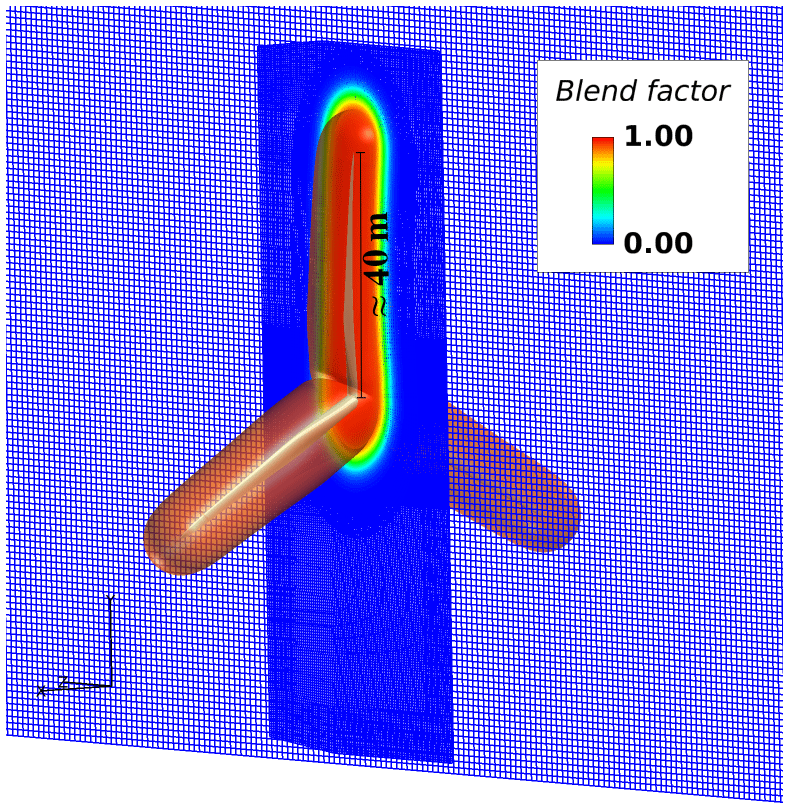
Figure 1 Blend factor, F_h. Red: IDDES region. Blue: Deardorff LES region. Isosurface of F_h=0.9 (≈6 m normal from surface).

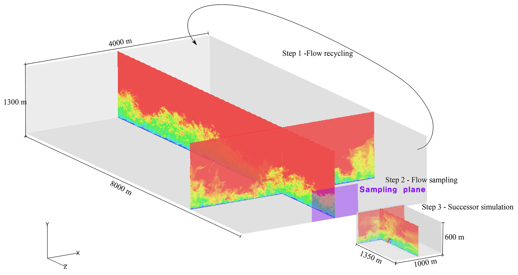
Figure 2 Concept of precursor to successor simulations along with domain sizes of conducted precursor and successor simulations. Colored contours showing flow velocity W.

2.3.2 HAWC2 model

The structural model used for the NM80 turbine was created and validated internally at DTU Wind Energy as part of the original DanAero project (Bak et al., 2013). This model was also used in a former study of FSI on the same rotor (Grinderslev et al., 2021) comparing URANS FSI with BEM-based aero-elastic simulations for complex laminar flow scenarios. The blade has a prebend into the wind of ≈1.5 m at the tip. Each blade is structurally discretized into 22 bodies, each consisting of one Timoshenko beam element. As only the rotor is modeled in CFD, only blade flexibility is considered as well. This means that tower, nacelle, shaft, and hub are not active parts of the HAWC2 simulations. A total of 60 aerodynamic sections are distributed per blade, which are used for both BEM and CFD loads. For BEM aerodynamics, airfoil data are used, obtained during the original DanAero project through wind tunnel tests and corrected for 3D effects; see Bak et al. (2006, 2011). From Grinderslev et al. (2021), it is known that the airfoil data do not capture well the 3D effects and predict an earlier stall than seen in CFD or experiments. In this case, however, the BEM calculations are used for initialization only to get good estimate of the initial bending, and for that reason no further corrections to the airfoil data have been conducted. Dynamic stall corrections (Hansen et al., 2004) and tip corrections (Glauert, 1935) are applied during the initializing BEM calculation. No controller is used, as a constant rotation speed of 16.2 rpm and pitch setting of −4.75^∘ (increasing the angle of attack) are set. For simplicity, the yaw and tilt are omitted in the simulation setup. For the DanAero campaign used for comparison, a tilt of 5^∘ and average yaw error of 6.01^∘ were present, however.

2.4 Simulation method

2.4.1 Precursor simulation

For the precursor simulation, as the first step, the turbulent flow is developed by recycling the flow using periodic boundary conditions. This resembles the flow moving over a very long distance, building up the boundary layer, and producing the turbulence through shear production. In order to ensure a mean profile close to the desired measured wind velocity profile, the SG wall model is used. This forces the surface shear stress of the first adjacent cells to the ground to fit the log law. The flow is driven trough a constant pressure gradient calibrated to obtain the desired friction velocity and resulting velocity profile with a roughness length z₀ of 0.73 m.

Initially, the grid sequencing scheme of EllipSys3D is utilized on three grid levels to speed up the simulation and reach a fully turbulent domain quickly. When the flow is fully turbulent and the mean flow profiles match the desired flow, planes consisting of velocity components U (horizontal perpendicular to mean flow direction), V (vertical and perpendicular to mean flow direction), and W (mean flow direction); pressure, P; and SGS kinetic energy, e, are sampled. The plane is centered in the cross-flow directions of 1000 m × 600 m with 4 m cell distances; see Fig. 2.

2.4.2 FSI simulation

The FSI successor simulation process is divided into phases depicted in Fig. 3.

Figure 3 Process diagram of conducted simulations.

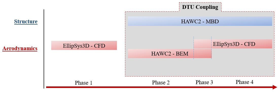
In the first phase, simulations without coupling to the structural solver are run to develop the flow and fill the domain with the sampled turbulent flow. In this phase, the grid sequencing scheme of EllipSys3D is used exploring coarser grids to minimize the simulation cost during spin-up.

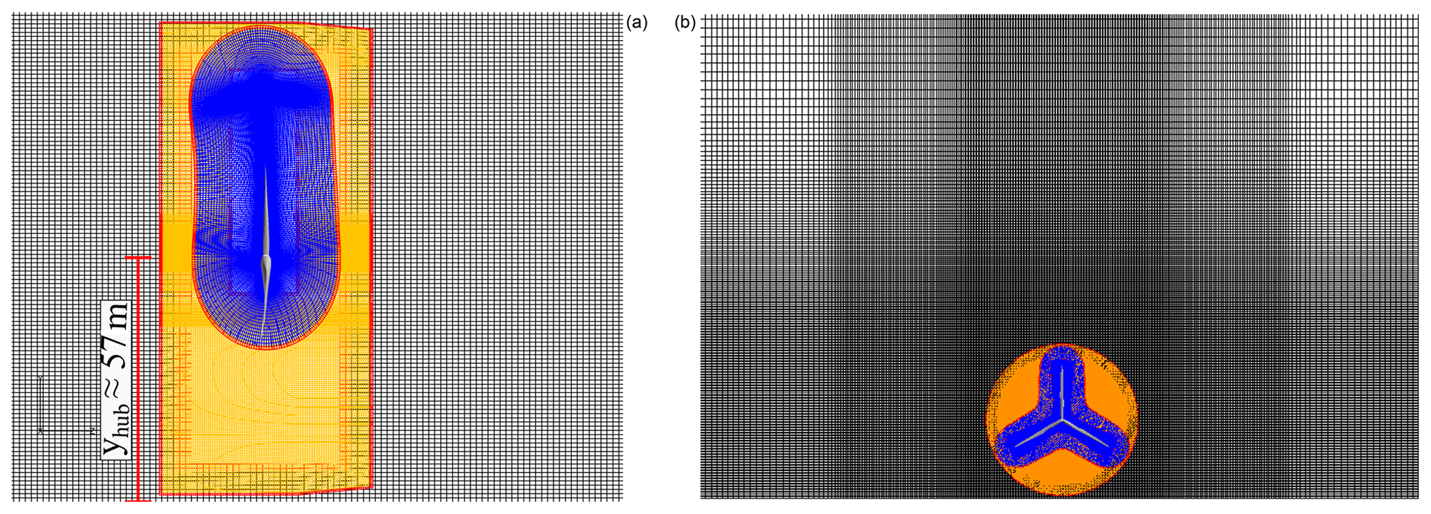
Figure 4 Grids used for simulations. (a) Side view, (b) front view. Red cells show receiver cells of overlapping grids. Blue: rotor grid. Orange: disc grid. Black: background grid. Entire background grid is not shown.

When passing to the FSI framework, phase 2, HAWC2 is run for the same amount of revolutions using BEM aerodynamics corresponding to the mean flow profile to ensure compatibility in time between the solvers when coupling and obtaining a good guess of initial blade deformations. In phase 3 the coupling of EllipSys3D and HAWC2 is initiated with a smooth linear blending of forces over two revolutions to switch from BEM to CFD loading. This is done to avoid any large force jumps in the HAWC2 solver, to suppress undesired vibrations in the system. In the final phase, phase 4, pure CFD loads are used for calculation of structural response, and a full two-way coupling is simulated for the desired amount of revolutions.

2.5 Computational grids

2.5.1 Precursor simulation

The precursor domain is $\mathrm{4000}\times \mathrm{1300}\times \mathrm{8000}$ m (width × height × length) discretized $\mathrm{576}\times \mathrm{256}\times \mathrm{1920}$ cells divided into 8640 blocks of 32³ cells. A total of ≈283 million cells are present in the precursor. The grid cells vary in size in the cross-flow directions to obtain higher resolution in the sampling area. In the sampling area, the cells are cubic with 4 m cell sides, while cells are slowly stretched towards the boundary sides and top. Periodic boundaries are prescribed on the vertical sides, while a symmetry condition is used on the top boundary, and the SG wall model is used for ensuring the Monin–Obukhov similarity law in the first cells adjacent to the wall by dictating the wall shear stress.

2.5.2 Successor simulation

For the rotor simulations, an overset grid method is utilized (Zahle et al., 2009), as this allows for a stationary background grid including the ground, while a rotating grid can be used for the rotor. Flow information is then communicated by interpolation between the grids through donor and receiver cells within the overlapping region of the meshes.

In the present setup, only the rotor is considered, omitting the tower, hub, and nacelle, with a total of three overlapping mesh groups; see Fig. 4. The omission of these elements is expected to have a minor effect, supported by Guma et al. (2021), who studied the same rotor represented both as a rotor only and as a full turbine. Near the rotor, an O–O type mesh is grown from the blade surface, extruding ≈15 m, discretized with 128 cells from the surface using the grid generator HypGrid (Sørensen, 1998). The first cell adjacent to the rotor surface has a height of $\mathrm{1}\times {\mathrm{10}}^{-\mathrm{6}}$ m to ensure a y⁺ of less than 1. Each blade is represented through 128 grid points spanwise and 256 chordwise. The blade tip and grid around a blade section are presented in Fig. 5. The rotor diameter, D, is ≈80 m.

Around the rotor mesh, a cylindrical disc mesh is constructed with pre-cut holes around the blades. This mesh rotates along with the rotor mesh, speeding up the hole-cutting algorithm, as the holes move along with the rotor. Thereby, the need of searching for hole, fringe, and donor cells between rotor and disc mesh for each time step is avoided, as the relations between the two meshes remain the same.

All deformation from the rotor is propagated to the rotor mesh in such a way that only cells that lie inside the hole region of the overlapping disc mesh deform. This is done to avoid deformation of the donor cells, keeping the interpolation coefficients between fringe and donor cells unaltered. Through this simplification, there is no need for updating communication tables for donor and receiver cells between the rotor and disc mesh as these also rotate together. This choice, however, necessitates that the hole of the disc mesh be far enough from the surface to leave room for the deformation of mesh cells without impairing the cell quality. In the present setup the holes are 17m wide in the rotor axis direction, where the main deformation is present, located with the undeformed rotor in the center. Displacements are propagated to the volume mesh, such that points within the inner 15 % of the grid curve length normal to the surface are moved as solid body motion to ensure no change of quality of the inner cells resolving the high gradient flow. Further out, from 15 to 40 % the volume blend factor is linearly decaying from 1 to 0, such that points from 40 % grid curve length and out are unchanged to avoid changes to donor cells. Note that communication tables and hole cutting still need an update between disc mesh and background mesh as the latter is static. The disc and rotor grids are similar to the setup used in Grinderslev et al. (2021); however in this study the background grid has changed to be suitable for LES simulations by using rectangular cells with low cell stretching in the area of focus.

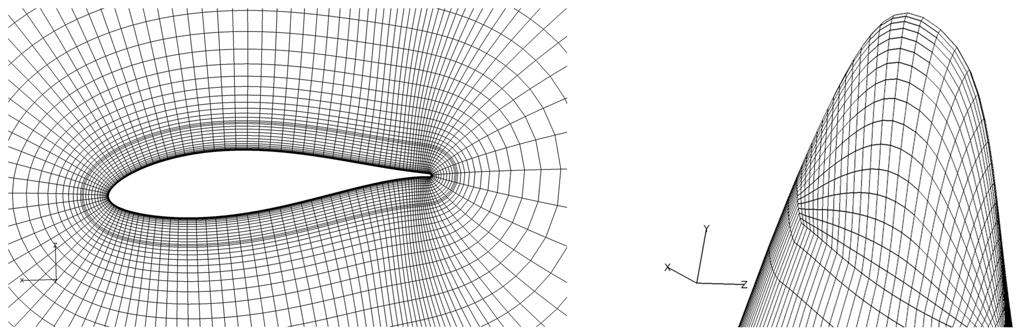
Figure 5 Near-rotor mesh at 25 m span and surface discretization at tip. Only every second line shown.

The background domain is a box of $\mathrm{1000}\times \mathrm{600}\times \mathrm{1350}$ m ($\mathrm{12.5}\times \mathrm{7.5}\times \mathrm{16.9}$ D) (width × height × length) using $\mathrm{352}\times \mathrm{256}\times \mathrm{640}$ cells, adding up to ≈58 million cells. A concentration of cells is present in the cross-flow directions around the rotor area down to 1 m side lengths; see Fig. 4 (right). Cells in the flow direction are kept constant at ≈1.4 m from the inlet to the rotor and 6 D behind it, before stretching towards the outlet. Boundary conditions are velocity inlet, outlet assuming fully developed flow, and symmetry conditions (slip walls) on sides and top boundaries. The ground has a no-slip wall condition, but with the SG wall model as in the precursor simulation. The rotor is placed ≈4.38 D from the inlet, ≈6.25 D from sides and top, and ≈12.5 D from the outlet.

A total of 78 million cells are used for the combined setup.

3 Results

3.1 Precursor simulation

A total of 9750 s was simulated for the precursor simulation, of which the final 1000 s (equivalent to ≈270 rotor revolutions) was sampled for statistical postprocessing, in a period where the developed flow profile sufficiently matched the desired profile. The precursor was run on three grid levels with varying time steps: first the coarse period ($\mathit{\delta }z=\mathit{\delta }y=\mathit{\delta }x\approx \mathrm{16}$ m, Δt=1.0 s), then a medium period ($\mathit{\delta }z=\mathit{\delta }y=\mathit{\delta }x\approx \mathrm{8}$ m, Δt=0.5 s), and finally a fine period ($\mathit{\delta }z=\mathit{\delta }y=\mathit{\delta }x\approx \mathrm{4}$ m, Δt=0.25 s). The full precursor simulation was conducted on 1728 AMD EPYC 2.9 GHz processors on the computer cluster of DTU and lasted ≈45 wall clock hours. The sampling was conducted in the fine phase only as depicted in Fig. 6 along with the pre-multiplied spectra f⋅S(f) at three different altitudes. As seen, the turbulence is well resolved with a decent inertial subrange following the Kolmogorov spectrum law with a decaying slope of $-\mathrm{2}/\mathrm{3}$.

Figure 6 (a) Time series of wind speed, W, at three altitudes, approximately matching the rotor bottom, center, and top altitudes. (b) Spectra of wind speed time series (fine-resolution period only) using the Welch estimate.

From the sampling plane, depicted in Fig. 2, the wind speed profiles of W were extracted and horizontally and temporally averaged ±1 D from the rotor position in the cross-plane direction as depicted in Fig. 7 (left). As seen, the relative difference of the averaged profile and the DanAero log-law fit match well with a maximum of 8 % at ≈14 m, which corresponds to only ≈0.5 m s⁻¹ at the specific altitude. One difference to note, however, is the larger standard deviation, and thus turbulence intensity, of the sampled flow, with fluctuations that supersede the DanAero measurements. The complexity of fitting both the mean profile and turbulence intensity between measurements and LES simulations is high. In this specific case, the assumption of neutral stratification in the simulation, with no knowledge about stratification being available from the measurements, likely plays a role in the capabilities to match results. This was the best match obtained after multiple calibration attempts, considering both mean profile and turbulence intensity.

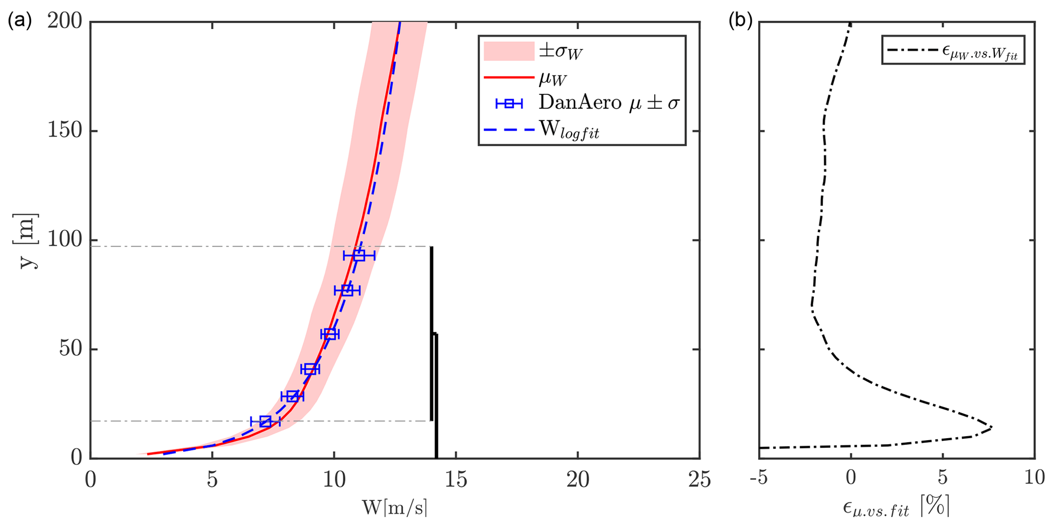
Figure 7 (a) Horizontal and temporal average profile μ_W ±1σ (solid red and red patch), DanAero measurements and fitted log law (blue error bars and dashed). Horizontal averaging based on flow from ±1 D from the rotor center on the sampled flow plane. (b) Relative error between log-law fit and μ_W profile.

Figure 8 depicts the resulting resolved and SGS flow shear stresses and resolved friction velocity, u^*.

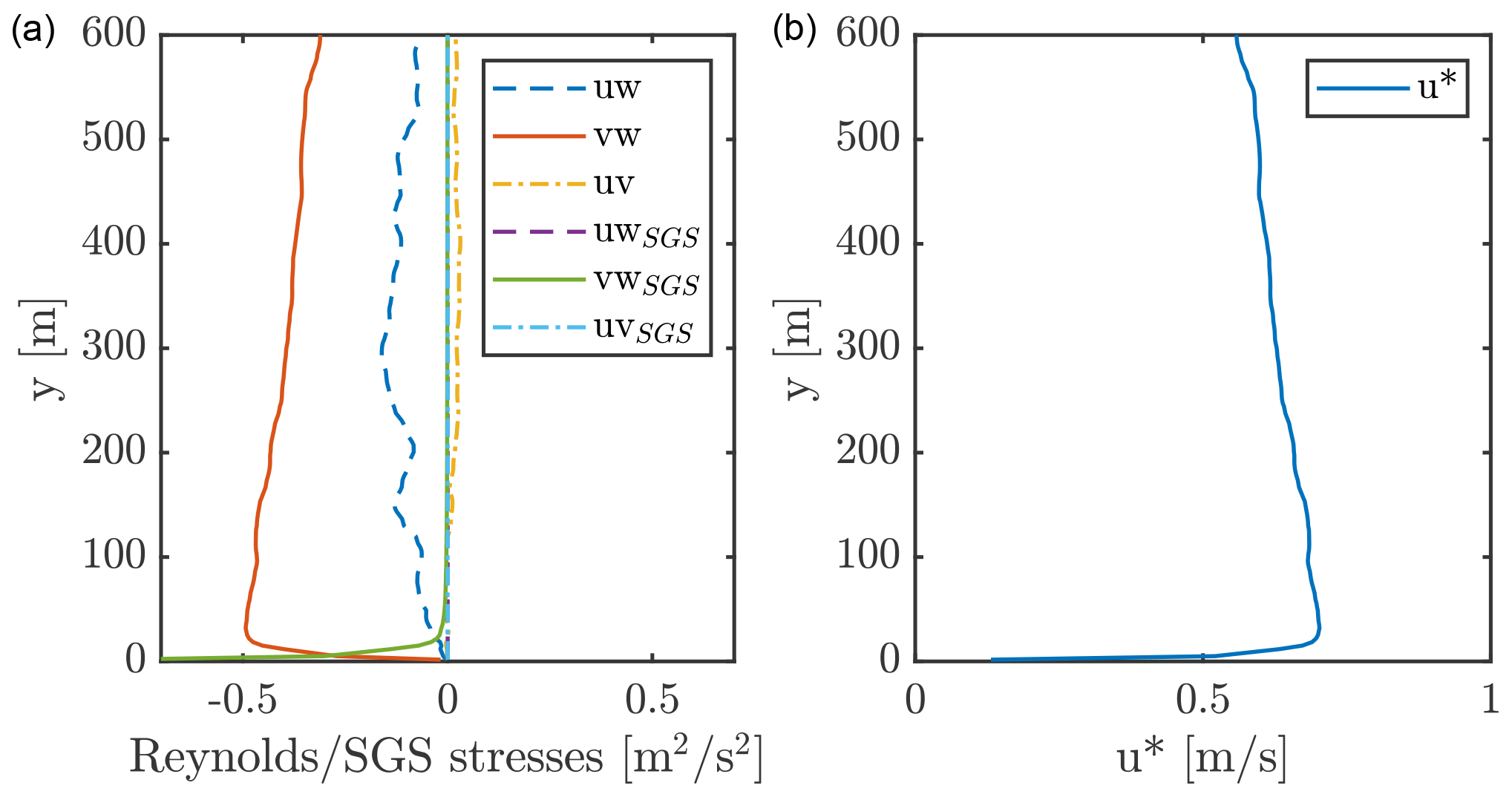
Figure 8 Precursor results: (a) horizontal averages of resolved and SGS shear stresses at 9250 s and (b) resulting resolved friction velocity $(u^{*}{)}^{\mathrm{2}}=\sqrt{v{w}^{\mathrm{2}}+u{v}^{\mathrm{2}}}$.

3.2 Successor simulation

In the following, the results of the successor simulations are presented. First, the new turbulence model is compared to the same setup using only the IDDES turbulence model assuming a elastically stiff configuration. Further, results from simulations using the hybrid model with and without flexibility of the blades are presented to study the effect of the blade elasticity. For the initial phase 1 (see Fig. 3), simulations were conducted on 1189 AMD EPYC 2.9 GHz processors, while coupled simulations (phases 3 and 4 in Fig. 3) were conducted on 793 Intel Xeon 2.8 GHz processors. The initialization simulations took on the order of ≈26 wall clock hours, while the coupled simulations lasted for ≈180 wall clock hours per simulation. Figure 9, shows the Q criterion = 0.4 (Hunt et al., 1988) of the flow, visualizing the turbulent structures up- and especially downwind of the rotor. As seen, the tip vortices in the wake are quickly broken up into smaller structures by the surrounding turbulent flow. This is also visible in Fig. 10, showing the flow velocity W at multiple downstream positions.

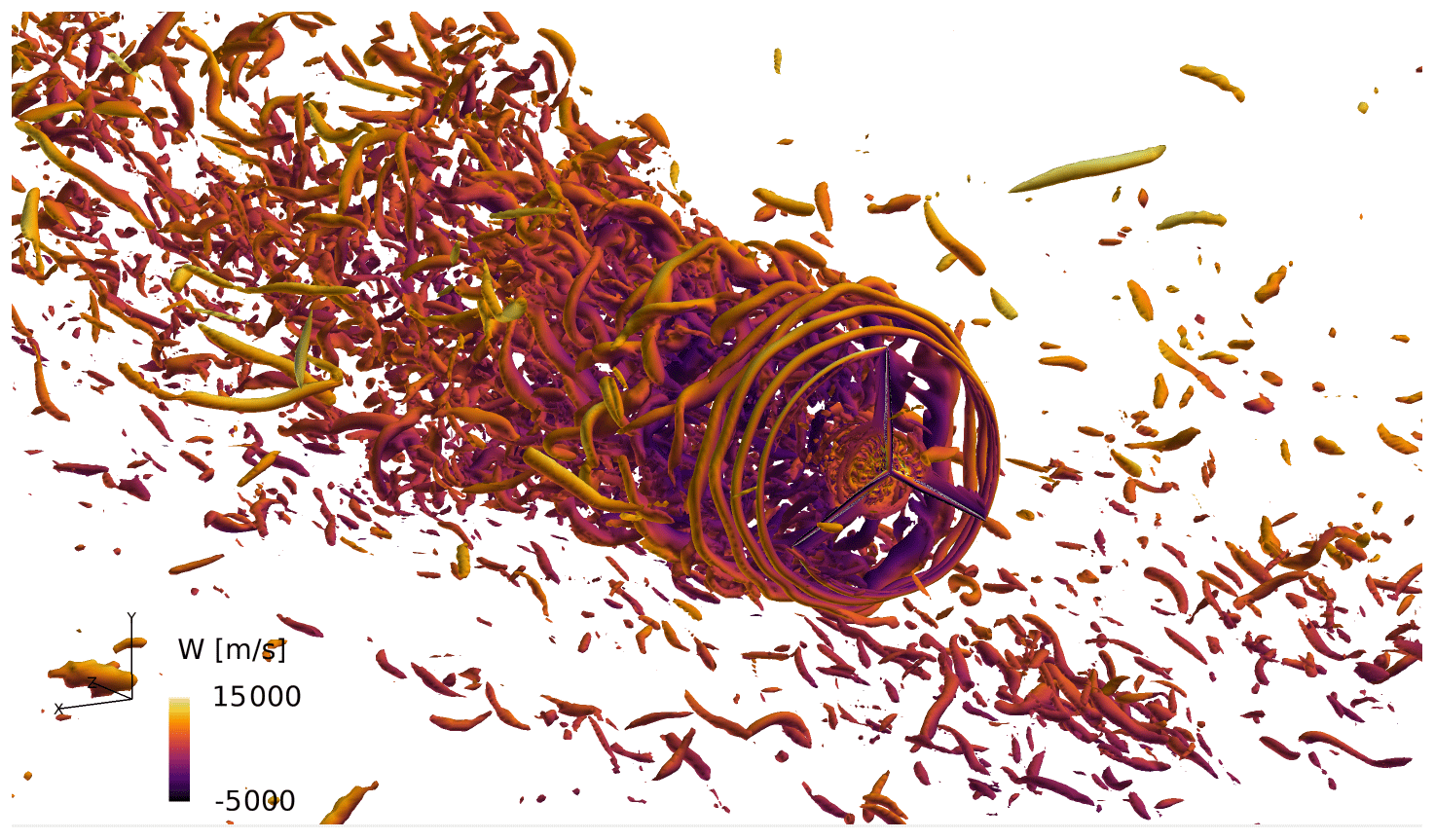
Figure 9 Isobars of Q criterion = 0.4 colored with value of flow velocity W, ranging from −5.0 to 15.0 m s⁻¹.

Figure 10 Velocity W downstream of rotor.

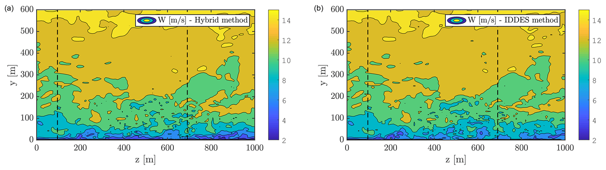
Figure 11 Instantaneous sections of flow velocity W for hybrid (a) and IDDES (b) simulations. Black dashed lines indicate the locations of the profiles presented in Fig. 12.

3.2.1 Impact of turbulence model

To study the impact of the presented turbulence model on the flow, simulations with the hybrid LES–IDDES blending enabled along with pure IDDES simulations are conducted. In the pure IDDES simulation, a slip wall condition is used on the terrain surface, contrary to the log law used for the LES–IDDES hybrid model. Simulations with and without the rotor present were simulated. In the empty setup, the hybrid model acts as a pure Deardorff LES model, as no blending region is defined. For all simulations, inflow is interpolated from the LES precursor planes to ensure identical inlet conditions. In the simulations comparing turbulence models, only the CFD code has been used, meaning that no flexibility of the blades is considered.

Firstly, the empty setups are presented in Fig. 11, showing the velocity component W at a vertical plane aligned with the flow direction intersecting the rotor center, for the simulations with Deardorff and IDDES turbulence modeling at the same time instance. From the planes, instantaneous velocity profiles and turbulence intensity profiles are extracted along the dashed lines, which are shown in Fig. 12. Both simulations show very comparable results. As seen, the velocity and TI profiles, extracted 96 m from the inlet, are practically identical, while a discrepancy is seen further downstream in the domain as a result of changing the turbulence and wall models. While both turbulence models perform close to identically for the present single-turbine-domain study, it could be speculated that this would not be the case when considering larger domains, for instance when studying multiple turbines at once. In that case, the differences in turbulence and wall modeling will likely result in different flow fields, due to the longer distances covered. Considering temperature effects on the flow might likewise reveal differences between the turbulence models. This could be in terms of temperature flux differences, along with the Deardorff model considering the stability in the mixing length scale, which is not the case in the IDDES model.

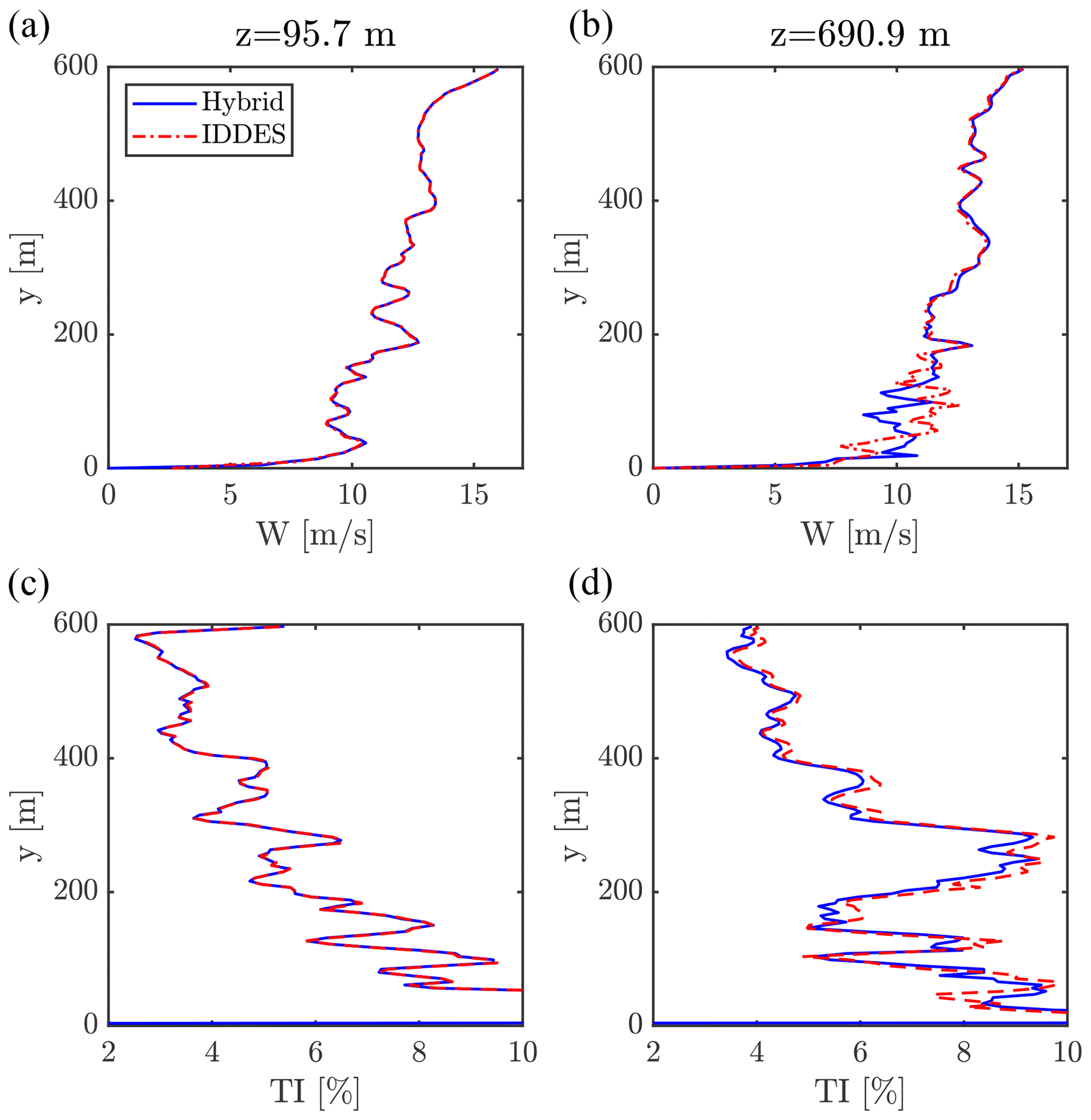
Figure 12 Instantaneous sampled profiles at time = 129.6 s. (a, b) Flow velocity W, (c, d) turbulence intensity (TI). Samples extracted from planes close to the inlet (96 m from inlet) and far downstream (691 m from inlet); see dashed lines of Fig. 11.

Stiff simulations covering 35 rotor revolutions were also conducted with the two turbulence models, including the rotor in the simulations. Mean and standard deviations of azimuthal forces of the final 15 revolutions at two blade sections, near the mid-span and near the tip, are presented in Fig. 13. Only slight differences are seen in both mean and standard deviations between the two models, aligning well with what is seen in the empty domain simulations. As the incoming flow is not altered significantly by the choice of turbulence model, and the turbulence model near the blade is IDDES in both simulations, the forces are expected to be similar as well.

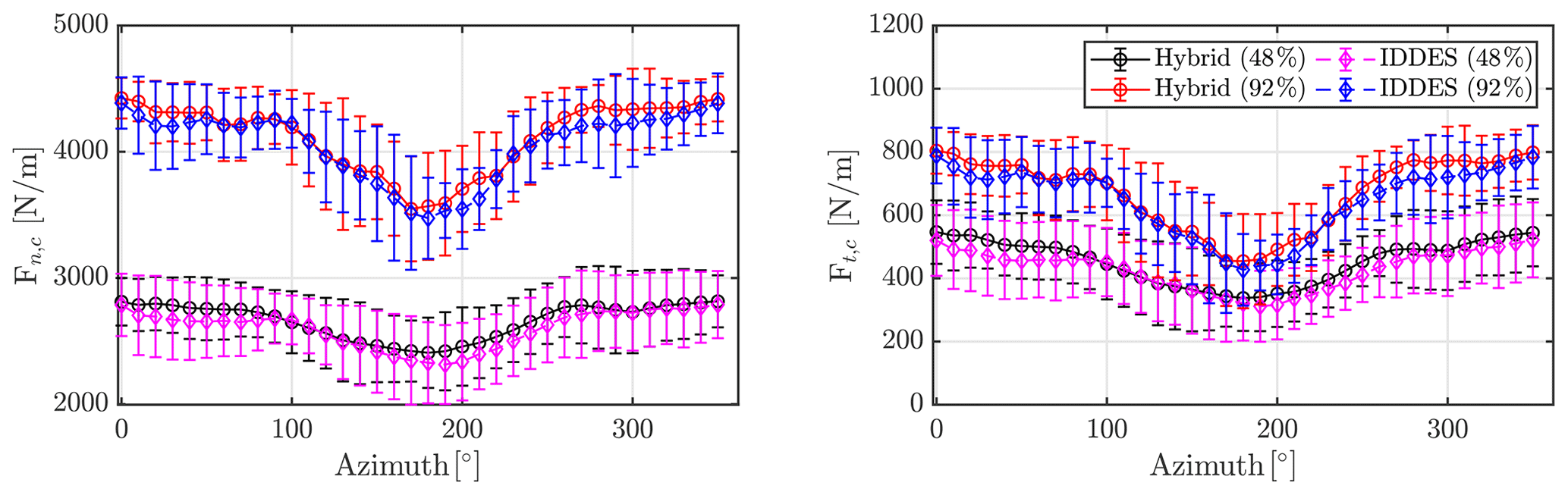
Figure 13 Normal and tangential forces at 48 and 92 % blade length using hybrid or IDDES turbulence model. Temporal means and standard deviations based on the final 15 revolutions.

3.2.2 Impact of flexibility

To study the effect of the rotor flexibility, FSI simulations of flexible and stiff setups were performed. First, 35 revolutions were simulated through pure CFD, as presented before, followed by 25 revolutions with the FSI coupling enabled; see Fig. 3 for the FSI simulation process.

The following results are obtained using the hybrid turbulence model only, but similar results would be expected for pure IDDES simulations, based on the aforementioned findings. The effect of including the blade flexibility is assessed through the resulting blade displacements, torsion, and rotor loading.

Figure 14 depicts the tip displacement flap- and edgewise along with the resulting blade torsion at 60.1 and 95.3 % blade length. The tip displacement in the flapwise direction is ≈6 % of the blade length, with fluctuations up to ≈1 % due to the turbulent flow. Edgewise displacements are low and dominated by gravity, seen in the more regular pattern and low standard deviation.

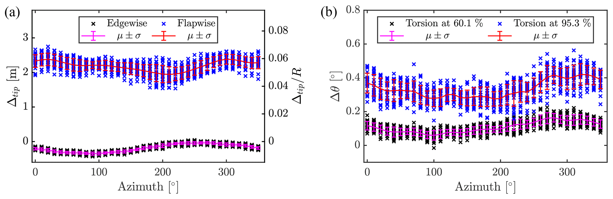
Figure 14 (a) Tip displacements flap- and edgewise. (b) Blade torsional deformation at 60.1 and 95.3 % blade length. Crosses represent instantaneous realizations.

Figure 15 Integrated thrust and torque for stiff and flexible configurations.

Blade torsion is quite low as well, with less than 0.5^∘ near the tip, increasing the angle of attack.

In Fig. 15, the integrated rotor thrust and torque are depicted, showing that in general only slight differences are seen by including flexibility. This is seen, with an increase in thrust of 1–5 %, while no significant change is seen in torque, other than a slight decrease in fluctuation amplitudes when including flexibility. The large- and small-scale fluctuations of the signals further indicate that the turbulent inflow has a higher impact on torque and thrust than the change seen from considering flexibility.

As mentioned, some differences are present in the simulation setup compared to the DanAero field experiment, being the omission of yaw, tilt, and tower along with the higher turbulence intensity of the generated flow.

Despite this disclaimer, the resulting forces at four sections of the blade are depicted in Fig. 16, showing the mean azimuthal pressure forces normal and tangential to chord for both flexible and stiff simulations along with the DanAero measurements. As seen, the forces agree well between the two simulations and the measurements, with the main differences being the lack of tower shadow at the inner sections, resulting in a drop of loading in the measurements not seen in the simulations (see Fig. 16, top row). The standard deviation of the forces is seen to be higher in simulations than for measurements, which is expected as the turbulence intensity of the sampled flow is higher than measurements as seen in Fig. 7.

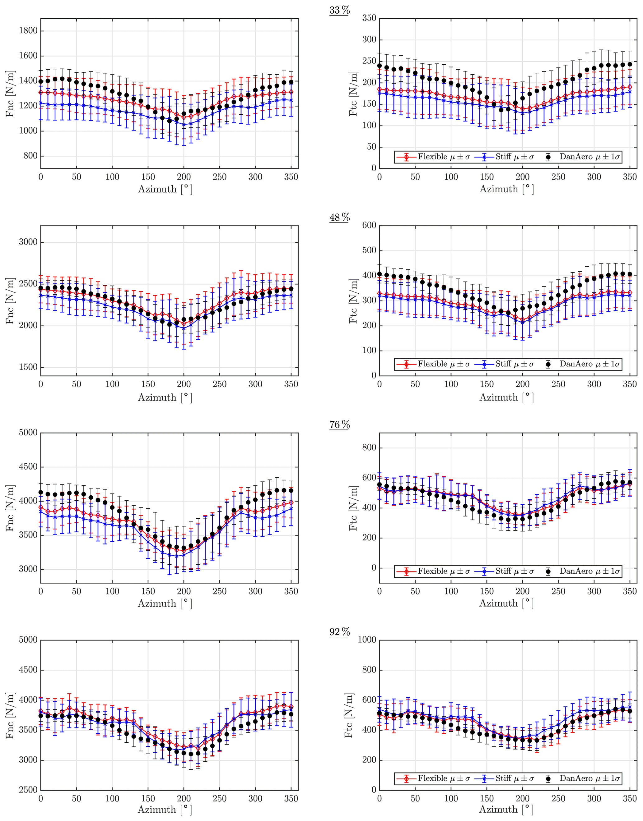
Figure 16 Normal and tangential forces for stiff and flexible simulations along with DanAero measurements. Sections at 33, 48, 76, and 92 % blade length.

The impact of including flexibility is quite small, and general observations are that normal and tangential forces respectively slightly increase and decrease when considering the flexibility of the rotor. This is expected for the NM80 rotor, which is quite stiff compared to modern wind turbines. The standard deviations of the forces due to turbulence are much higher than the difference between mean forces of stiff and flexible simulations. This shows that including turbulent inflow is more important than including flexibility, at least in the present rotor/flow case. In the simulations including the flexibility the standard deviations of the normal forces are up to 10 % of the mean near the tip and 15% near the root. For tangential forces this is even higher, with 24 % near the tip and 38 % near the root.

Spectral analysis of the resulting normal and tangential force signals at the 76 % blade length section are presented in Fig. 17 (left), showing the power spectral densities (PSDs) using the Welch estimate. As seen, both stiff and flexible simulations result in similar PSDs, with the main difference being the peak at the first edgewise frequency seen in the flexible signal. The majority of energy is found in the rotation frequency, 1P, and its harmonics. This is also the case when looking at the PSD of the tip displacement in the flap- and edgewise direction. Here, it is again the rotation frequency and its harmonics that dominate, along with a peak of the first edgewise mode.

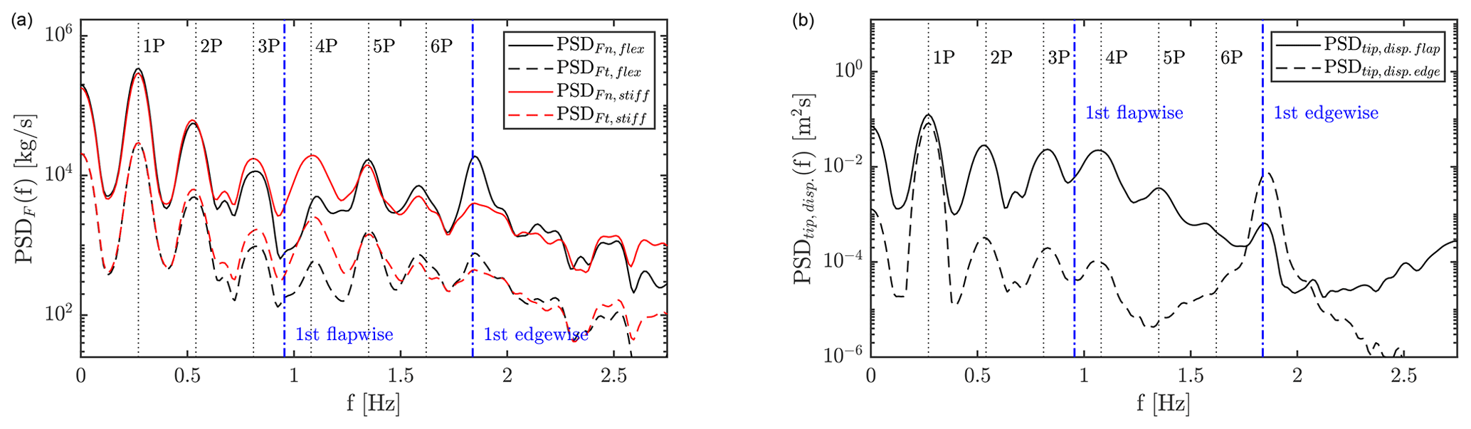
Figure 17 (a) PSD of normal and tangential forces at 78 % blade length for both stiff and flexible simulations. (b) PSD of tip displacement in flap- and edgewise direction.

4 Conclusions

This study investigates the phenomenon of aero-elasticity of wind turbines placed in atmospheric flow conditions, by means of high-fidelity numerical methods. Fluid–structure interaction (FSI) simulations of a 2.3 MW wind turbine rotor have been conducted using a novel turbulence model, blending the Deardorff large-eddy simulation (LES) model for atmospheric flows with the improved delayed detached eddy simulation (IDDES) model for the separated flow near the rotor boundary. Precursor simulations were conducted in a large domain in order to assure sampling of realistic turbulent atmospheric boundary layer (ABL) flow, matching well with the DanAero measurements, for the successor simulations.

As the first study, the hybrid model was compared to the pure IDDES turbulence model, by computational fluid dynamics (CFD) successor simulations of the turbulent ABL inflow with and without the rotor present. In empty simulations, this corresponded to a comparison between pure Deardorff LES and pure IDDES, while for rotor simulations the hybrid model used both Deardorff LES for the domain flow and IDDES for the near-rotor flow. It was found that there was no significant difference in either the flow or the rotor loading between the two methods, likely due to the short domain considered and assumptions omitting the Coriolis force and temperature effects.

Secondly, FSI simulations were conducted by coupling the CFD simulations to a structural solver. It was found that for the specific rotor, which is relatively stiff compared to modern turbines, only a small impact was found by considering the flexibility of the blades. A general increase of ≈1–5 % in total thrust was found, while the power producing torque was close to identical for stiff and flexible simulations.

Inflow turbulence on the other hand has a large influence on the rotor loading, with standard deviations as high as 15 % of the mean for normal forces and even higher tangentially. This emphasizes the importance of correct modeling of inflow turbulence.

5 Future studies

As has been shown in the present study, the developed hybrid turbulence model resulted in practically identical loading of the rotor to that of the IDDES model alone. Relevant future studies would be to investigate when this is not the case. This could for instance be simulations including stable/unstable stratification and/or the Coriolis force. Here, the IDDES model will probably be insufficient to capture the effects, as the model is calibrated for aerodynamics mainly and not ABL flows. The Deardorff LES model, however, is calibrated for such flows, and the mixing length scale depends on the stratification, as it is reduced for stable cases. The two models also model temperature effects differently as the flux (τ_θ,w) is based on different weights of the turbulent viscosity. Longer domains with multiple rotors could also be relevant, as there are time and distance for the two turbulence models to develop the flow differently, which is indicated by the results of the present study.

A relevant future study would likewise be to compare the method to more efficient BEM-based aerodynamics solvers with the precursor turbulence as input. Here, the CFD-based results could, if needed, be used to correct airfoil polars and calibrate the many correction models needed by BEM solvers to consider e.g. tip loss effects, dynamic inflow, and dynamic stall.

In terms of FSI, it would be natural to investigate more recent/future turbine designs, which are larger and much more flexible than the considered NM80 rotor. These rotors are at a higher risk of instability phenomena and operate in a larger part of the atmospheric boundary layer.