the Creative Commons Attribution 4.0 License.
the Creative Commons Attribution 4.0 License.
 | 21 May 2021
Control-oriented model for secondary effects of wake steering
Jennifer King
Paul Fleming
Ryan King
Luis A. Martínez-Tossas
Christopher J. Bay
Rafael Mudafort
Eric Simley
This paper presents a model to incorporate the secondary effects of wake steering in large arrays of turbines. Previous models have focused on the aerodynamic interaction of wake steering between two turbines. The model proposed in this paper builds on these models to include yaw-induced wake recovery and secondary steering seen in large arrays of turbines when wake steering is performed. Turbines operating in yaw-misaligned conditions generate counter-rotating vortices that entrain momentum and contribute to the deformation and deflection of the wake at downstream turbines. Rows of turbines can compound the effects of wake steering that benefit turbines far downstream. This model quantifies these effects and demonstrates that wake steering has greater potential to increase the performance of a wind farm due to these counter-rotating vortices especially for large rows of turbines. This is validated using numerous large-eddy simulations for three-turbine, five-turbine, and wind farm scenarios.
- Article
(3071 KB) - Full-text XML
- BibTeX
- EndNote


Wake steering is a type of wind farm control in which wind turbines in a wind farm operate with an intentional yaw misalignment to mitigate the effects of its wake on downstream turbines in order to increase overall combined wind farm energy production (Wagenaar et al., 2012). To design model-based controllers for wake steering, engineering models of the aerodynamic interactions between turbines are needed. Engineering models, in this context, are computationally efficient models that include enough physics to predict wake steering behavior while running fast enough to be optimized in real time. These models can then be used in the design of wind farm control strategies (Simley et al., 2019; Fleming et al., 2019), layout optimizations (Gebraad et al., 2017; Stanley and Ning, 2019), or real-time control (Annoni et al., 2019).
An early model of wake steering was provided in Jiménez et al. (2010). This model was combined with the Jensen model (Jensen, 1984) in the multi-zone wake model in FLORIS (Gebraad et al., 2016). The model was compared with large-eddy simulations (LESs) using the Simulator for Wind Farm Applications (SOWFA, Churchfield et al., 2014), and several additional corrections including division of the wake into separate zones were added to better capture the aerodynamic interactions.
Several recent papers proposed a new wake deficit and wake deflection model based on Gaussian self-similarity (Bastankhah and Porté-Agel, 2014, 2016; Niayifar and Porté-Agel, 2015; Abkar and Port-Agel, 2015). This model includes added turbulence due to the turbine operation that influences wake recovery (Crespo et al., 1999). In addition, this model has some tuning parameters and includes atmospheric parameters that can be measured such as turbulence intensity (Niayifar and Porté-Agel, 2015). This model is commonly referred to as the Bastankhah model, EPFL model, or Gaussian model. We will use the term Gaussian for the remainder of the paper. The Gaussian model was included as a wake model within the FLORIS tool (NREL, 2019). It has been used to design a controller for a field campaign in Fleming et al. (2019) and study wake steering robustness (Simley et al., 2019), and it has been validated with lidar measurements (Annoni et al., 2018). The Gaussian model is also used in wind farm design optimization in Stanley and Ning (2019).
One of the main issues observed with the Gaussian model in FLORIS is that the model tends to under-predict gains in power downstream with respect to LES and field data. In addition, Fleming et al. (2016) and Schottler et al. (2016) show wake steering is asymmetrical; i.e., clockwise and counterclockwise yaw rotations do not produce equal benefits at the downstream turbine. An empirical term had been explored to address this in Gebraad et al. (2016); however, it still does not fully capture the asymmetries present in the wake of yaw-misaligned turbines.
Fleming et al. (2018a) investigates the importance of considering explicitly the counter-rotating vortices generated in wake steering (Medici and Alfredsson, 2006; Howland et al., 2016; Vollmer et al., 2016) to fully describe wake steering in engineering models. These vortices deflect and deform the wake at the downstream turbine. It is also noted in Fleming et al. (2018a) that these vortices persist farther downstream and impact turbines that are third, fourth, etc. in the row. This is known as secondary steering. It was proposed that modeling the counter-rotating vortices generated in wake steering could provide a means to model this process and how wake steering will function when dealing with larger turbine arrays. Further, Ciri et al. (2018) has shown that modeling/accounting for the size of these vortices versus the length scales in the atmospheric boundary layer explains variations of the performance of wake steering for differently sized rotors.
Martínez-Tossas et al. (2019) provides a wake model, known as the curl model, which explicitly models these vortices. The paper shows that modeling the vortices can predict the deflection of the wake in misaligned conditions as well as the change in wake shape and cross-stream flows observed in Medici and Alfredsson (2006), Howland et al. (2016), Vollmer et al. (2016), and Fleming et al. (2018a). However, the Reynolds-averaged Navier–Stokes (RANS)-like implementation of the curl model and finite-difference solution scheme significantly increases the computation complexity (around 1000×).
This paper presents a hybrid wake model, which modifies the Gaussian model (Bastankhah and Porté-Agel, 2014, 2016; Niayifar and Porté-Agel, 2015), with analytic approximations made of the curl model in Martínez-Tossas et al. (2019). This hybrid model will be referred to as the Gauss–curl hybrid, or GCH model. We propose it as a compromise which maintains the many advantages of the Gaussian model while incorporating corrections to address the following three important discrepancies.
-
Vortices drive a process of added yaw-based wake recovery, which increases the gain from wake steering to match LES and field results.
-
The interaction of the counter-rotating vortices with the atmospheric boundary layer shear layer and wake rotation induces wake asymmetry naturally.
-
By modeling of the vortices, secondary-steering and related multi-turbine effects are included, which will be important for evaluating wake steering for large wind farms.
In this paper, we will introduce the analytical modifications made to the Gaussian model in Sect 2. We will use numerous LESs to show that the improvements made in GCH resolve the discrepancies identified above. This model will demonstrate how it compares with LES of three turbines (Sect. 3), five turbines (Sect. 4), and a 38-turbine wind farm (Sect. 5). In addition to these simulations, the proposed model is also validated using the results of a wake steering field campaign at a commercial wind farm (Fleming et al., 2020).
This section briefly describes the Gaussian model used to describe the velocity deficit and the effects of wake steering in a wind farm. Figure 1 shows the setup for the control-oriented model described in this paper. It is noted that mass and momentum are not conserved quantities in this model, which is the subject of ongoing research.
The proposed model, known as the Gauss–curl hybrid (GCH) model, builds upon the Gaussian model introduced in Bastankhah and Porté-Agel (2016), Abkar and Porté-Agel (2014), Abkar and Port-Agel (2015), and Niayifar and Porté-Agel (2015) by including entrainment, asymmetry, and secondary wake steering effects seen in LES as well as field results.
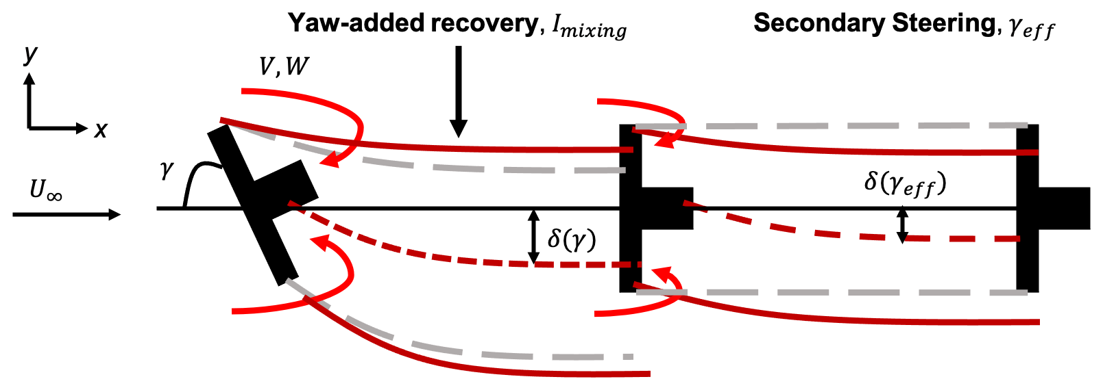
Figure 1Model setup that includes yaw-induced effects such as yaw-added recovery and secondary steering. The standard modeling for wake deflection is shown in gray, and the proposed deflection model in this paper is shown in red. These effects manifest through the spanwise and vertical velocities that are generated from yaw-misaligned turbines. These effects are described in Sect. 2.2.
2.1 Velocity deficit model
The wind turbine wake model used to characterize the velocity deficit behind a turbine in normal operation in a wind farm was introduced by several recent papers including Bastankhah and Porté-Agel (2016), Abkar and Port-Agel (2015), Niayifar and Porté-Agel (2015), and Bastankhah and Porté-Agel (2014). The velocity deficit of the wake is computed by assuming a Gaussian wake, which is based on self-similarity theory often used in free shear flows (Pope, 2000). An analytical expression for the streamwise velocity, uG, behind a turbine is computed as
where C is the velocity deficit at the wake center, U∞ is the freestream velocity, δ is the wake deflection (see Sect. 2.1.1), y0 is the spanwise position of the turbine, zh is the hub height of the turbine, σy defines the wake width in the y direction, and σz defines the wake width in the z direction. The subscript “0” refers to the initial values at the start of the far wake, which is dependent on ambient turbulence intensity, I0, and the thrust coefficient, CT. For additional details on the onset of the far-wake calculations, the reader is referred to Bastankhah and Porté-Agel (2016). Abkar and Port-Agel (2015) demonstrate that the wake expands at different rates based on lateral wake meandering (σy direction) and vertical wake meandering (σz direction). The velocity distributions σz and σy are defined as
where D is the rotor diameter, uR is the velocity at the rotor, u0 is the velocity at the start of the far wake, ky defines the wake expansion in the lateral direction, and kz defines the wake expansion in the vertical direction. For this study, ky and kz are set to be equal, and the wake expands at the same rate in the lateral and vertical directions. The wakes are combined using the traditional sum-of-squares method (Katić et al., 1986), although alternate methods are proposed in Niayifar and Porté-Agel (2015).
This wake model also computes added turbulence generated by turbine operation and ambient turbulence conditions. For example, if a turbine is operating at a higher thrust, this will cause the wake to recover faster. Conversely, if a turbine is operating at a lower thrust, this will cause the wake to recover slower. Conventional linear flow models have a single wake expansion parameter that does not change under various turbine operating conditions. Niayifar and Porté-Agel (2015) provided a model that incorporated added turbulence due to turbine operation. Added turbulence is computed using (Crespo et al., 1999)
where I is the ambient turbulence intensity. The values used in this equation are slightly different from those in Niayifar and Porté-Agel (2015) and have been tuned to large-eddy simulations.
Wake deflection
In addition to the velocity deficit, a wake deflection model is used to describe the flow behavior behind a yaw-misaligned turbine, which occurs when performing wake steering and is also implemented based on Bastankhah and Porté-Agel (2016). The initial angle of wake deflection, θ, due to yaw misalignment is defined as
The initial wake deflection, δ0, is then defined as
where x0 indicates the length of the near wake. This can be computed analytically based on Bastankhah and Porté-Agel (2016).
The total deflection of the wake due to yaw misalignment is defined as
where . See Bastankhah and Porté-Agel (2016) for details on the derivation. The tuning parameters used in this paper are consistent with values from Bastankhah and Porté-Agel (2016) and Niayifar and Porté-Agel (2015).
2.2 Spanwise and vertical velocity components
The spanwise and vertical velocity components are currently not computed in the Gaussian model, but they are critical components for modeling the effects of wake steering. These velocity components can be computed based on wake rotation and yaw misalignment as shown in Martínez-Tossas et al. (2019) and Bay et al. (2019).
Wake rotation is included by modeling a Lamb–Oseen vortex, which makes sure that the vortex is not a singular point near the center of the rotor. The circulation strength for the wake rotation vortex is now
where a is the axial induction factor of the turbine, and λ is the tip-speed ratio, which is assumed to be a user input, i.e., not computed within the FLORIS framework. See Martínez-Tossas et al. (2019) for additional details. Axial induction can be mapped to CT using (Bastankhah and Porté-Agel, 2016)
The vertical and spanwise velocities can then be computed using the strength of the vortex, Γ, by
where y0 is the spanwise position of the turbine, ϵ represents the size of the vortex core. In this paper, ϵ=0.3D, which is similar to Martínez-Tossas et al. (2019).
In addition to the wake rotation, when a turbine is operating in yaw-misaligned conditions, the turbine generates a collection of smaller counter-rotating vortices that are approximated as one pair of large counter-rotating vortices that are released at the top and the bottom of the rotor and generate additional spanwise and vertical velocity components that need to be accounted for in this approach (Martínez-Tossas et al., 2019; Shapiro et al., 2018). The strength of these vortices, Γ, can be computed as and is a function of the yaw angle, γ (Martínez-Tossas et al., 2019):
where ρ is the air density.
As is done with wake rotation, the spanwise and vertical velocity components, V and W, are computed based on the strength of the yaw misalignment of a turbine. The spanwise velocity can be computed as
where Vtop and Vbottom are velocity deficit functions that originate from the rotating vortex at the top and bottom of the rotor, respectively. Γtop and Γbottom are computed using the velocity at the top and bottom of the rotor based on the shear present at the rotor. In general, Γtop will be stronger than Γbottom.
The spanwise and vertical velocities are combined using a linear combination at downstream turbines as is done in Martínez-Tossas et al. (2015) and Bay et al. (2019). The total spanwise velocity is
Similarly, the vertical velocity can be written as
The total vertical velocity can be computed as
Note that ground effects are included by adding mirrored vortices below the ground as is done in Martínez-Tossas et al. (2019).
Finally, the vortices generated by the turbines decay as they move downstream. The dissipation of these vortices is described in Bay et al. (2019) and can be computed as
where νT is the turbulent viscosity, which is defined using a mixing length model:
where , κ=0.41, and . λT is the value of the mixing length in the free atmosphere (Pope, 2000).
2.3 Added wake recovery due to yaw misalignment
The streamwise velocity and the wake deflection are influenced by the spanwise and vertical velocity components, V and W. First, the wake recovers more when the turbine is operating in misaligned conditions due to the large-scale entrainment of flow into the wind farm domain. In this paper, we include yaw-added recovery (YAR) as an added mixing term that influences the wake recovery σy and σz in the Gaussian model.
In Martínez-Tossas et al. (2019), it is assumed that the mean values of the spanwise and vertical velocities are small, and we assume that the fluctuations in the spanwise and vertical directions are on the same order as the mean. The fluctuations induced by the counter-rotating vortices are defined in Eqs. (20) and (21) above. The fluctuations influence the turbulent kinetic energy (TKE) that ultimately impacts the wake recovery. TKE, k, is defined as (Pope, 2000)
where is determined from the ambient turbulence intensity defined; is the average V fluctuations at a turbine, assumed to be small; vcurl is determined by Eq. (20); is the average W fluctuations at a turbine, assumed to be small; and wcurl is determined by Eq. (21).
In particular, u′ is determined by converting the ambient turbulence intensity into TKE by (Stull, 2012)
where is the average streamwise velocity at a turbine, and I is the turbulence intensity at a turbine. The streamwise fluctuations are then computed as
The TKE is converted to a turbulence intensity through the following (Stull, 2012):
where Ui is the average velocity at turbine i. The amount of turbulence generated from the counter-rotating vortices can be calculated by
where I is the ambient turbulence.
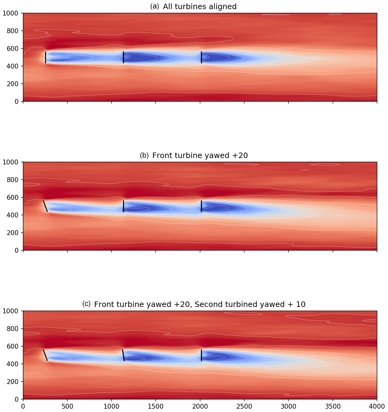
Figure 2Three-turbine array in SOWFA where all turbines are aligned (a), the first turbine is yawed +20∘ (b), and the first turbine is yawed +20∘ and the second turbine is yawed +10∘ (c).
Incorporating secondary steering effects by the introduction of an effective yaw angle
In addition to added wake recovery, the model proposed in this paper is able to predict secondary steering that matches large-eddy simulations. The wake deflection model described in Sect. 2.1.1 can be used to describe the deflection of the wake for a two-turbine case. However, additional information is needed to describe the impact of yaw misalignment on turbines in large wind farms as is shown in Fleming et al. (2018a).
Specifically, the vortices described in the previous section propagate far downstream, dissipate, and affect all turbines directly downstream of the turbine that generated the vortices. When they reach a downstream turbine, they impact the wake of the downstream turbine in a phenomenon called secondary steering (Fleming et al., 2018b). The spanwise and vertical velocities generated by the counter-rotating vortices act like an effective yaw angle at the next turbine. In other words, the spanwise and vertical velocity components of upstream turbines affect the deformation and deflection of a wake downstream as if the downstream turbine were implementing wake steering even when it is aligned with the flow. In this model, these effects are approximated as an effective yaw angle. To model secondary steering, an effective yaw angle is computed to describe the effect of the vortices generated at the upstream turbine on the downstream turbine wake. The effective yaw angle is computed using the mean spanwise velocity, V, present at the turbine rotor. The effective yaw angle, γeff, is computed by finding the yaw angle that reproduces the approximate spanwise velocity:
where γ is an array of yaw angles between and . This determines what the yaw angle of the turbine would have needed to be to produce that same spanwise velocity. The effective yaw angle, γeff, is found by minimizing the difference between the effective spanwise velocity and the spanwise velocity calculated at the rotor:
The total wake deflection can be computed using Eq. (8), where the total yaw angle, γ, is
where γturb is the amount of yaw offset the turbine is actually applying. This γ is used in Eq. (8) to compute the lateral deflection of the wake.
Due to the presence of the effective yaw angle, downstream turbines generally do not have to yaw as much as upstream turbines to produce large gains. This phenomenon was observed in a wind tunnel study (Bastankhah and Porté-Agel, 2019).
The addition of yaw-added recovery and secondary steering effects has increased the computational time by 3.5 times, e.g., a five-turbine case takes 0.007 s to run the GCH model compared to 0.002 s for the Gaussian model. However, the results in this paper indicate that when evaluating wake steering, GCH is necessary to include as the Gaussian model is not able to capture the compounding effects of wake steering.
First, the Gaussian model, GCH model, and SOWFA are compared in three-turbine array simulations. The three-turbine array demonstrates the benefits of the yaw-added recovery (YAR) effect as well as secondary steering (SS). The following plots show the contributions of YAR and SS compared with the Gaussian model and the full GCH model, which contains both YAR and SS. The YAR and SS models are computed by disabling the model produced in Sect. 2.3 within the GCH model to isolate the two effects.
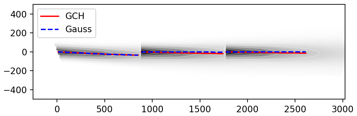
Figure 3FLORIS results for the three-turbine case shown for the GCH model with the centerline of the wake computed for GCH (red) and the Gaussian model (blue), where the first turbine is yawed 20∘.
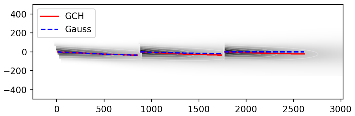
Figure 4FLORIS results for the three-turbine case shown for the GCH model with the centerline of the wake computed for GCH (red) and the Gaussian model (blue), where the first turbine is yawed 20∘ and the second turbine is yawed 10∘.
The three-turbine scenario was simulated at 8 m/s with 6 % and 10 % turbulence intensities and spaced 7D apart in the streamwise direction. Figure 2 shows the flow fields from the SOWFA simulations for the baseline (top row), the first turbine yawed 20∘ (middle row), and the first turbine yawed 20∘ and the second turbine yawed 10∘ (bottom row). For visual comparison, Figs. 3 and 4 show FLORIS computed using the GCH model where the first turbine is yawed 20∘ (Fig. 3) and the first turbine is yawed 20∘ and the second turbine is yawed 10∘ (Fig. 4). The impact of secondary steering is shown in the wake centerlines where the Gaussian model centerline is shown in blue and the wake centerline computed with GCH is shown in red. It can be seen that there is steering on downstream turbines that are not yawed in the GCH model, and there is no movement in the wake centerline in non-yawed turbines in the Gaussian model.
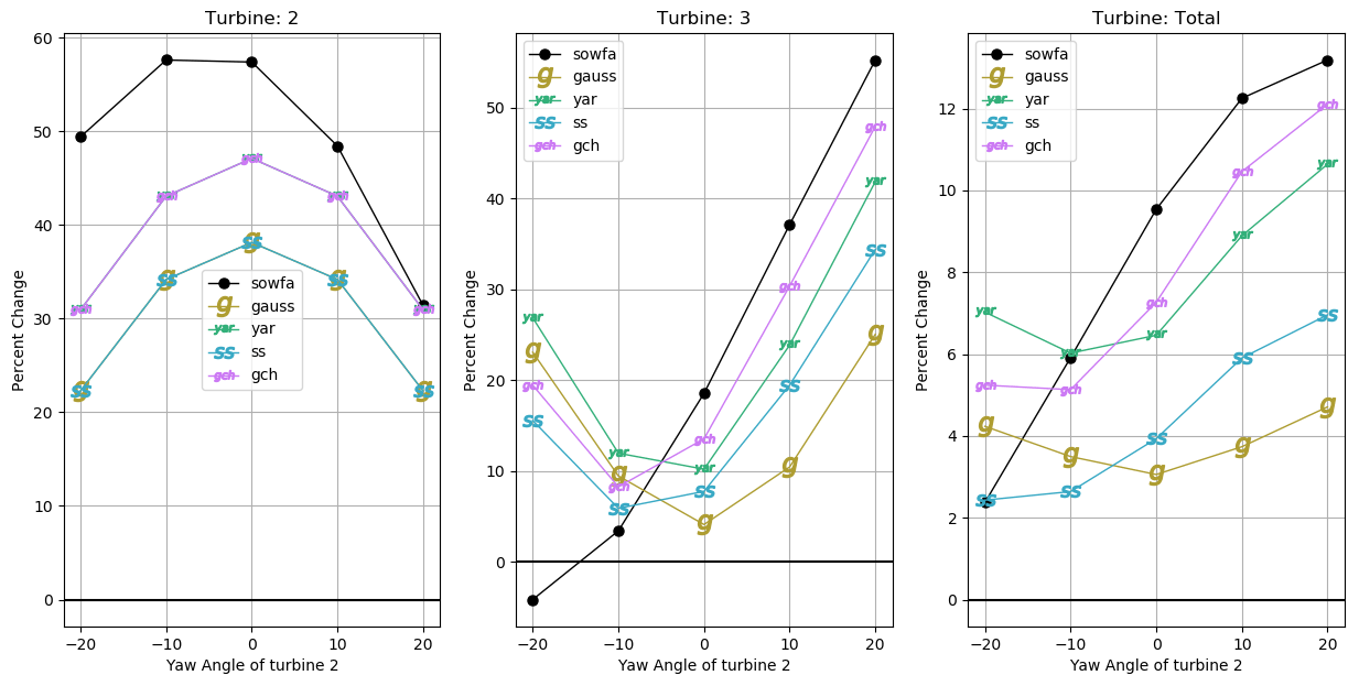
Figure 5Comparison of changes in power when sweeping the angle of the second turbine, i.e., Turbine 2, when the angle of the first turbine, i.e., Turbine 1, is set to +20∘ where the wind speed was 8 m/s and the turbulence intensity was 6 %. The results of the change in power of the third turbine, as well as the overall total of all three turbines, reflect the importance that the two yaw offsets are in the same direction.
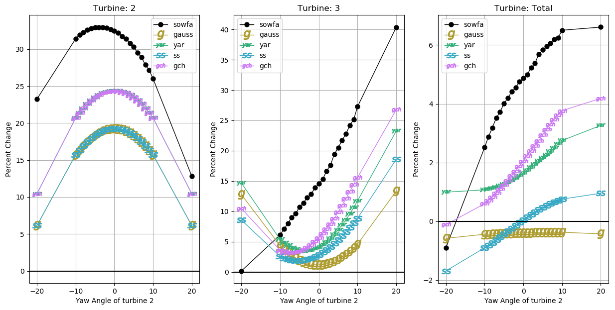
Figure 6Comparison of changes in power when sweeping the angle of the second turbine, i.e., Turbine 2, when the angle of the first turbine, i.e., Turbine 1, is set to +20∘ where the wind speed was 8 m/s and the turbulence intensity was 10 %.
Next, several simulations were run at each turbulence intensity where the first turbine was yawed 20∘ and the second turbine was yawed between and +20∘. Figures 5 and 6 show the relative power gains of the SOWFA simulations for turbulence intensities of 6 % and 10 % respectively relative to a baseline case of all turbines aligned. The SOWFA simulations are compared with the Gaussian model, YAR, SS, and the GCH model. The power gains of Turbine 2 are shown in the left plot in Figs. 5 and 6, Turbine 3 is shown in the middle plot, and the total power gains are shown in the right plot.
The Gaussian model is not able to capture the secondary effects of wake recovery and secondary steering. The Gaussian model is able to capture gains in low-turbulence (6 %) conditions; see Fig. 5. However, it does not see any gains when turbulence intensity is higher as shown in Fig. 6. It is also important to note that for Turbine 3 and the total gains, the Gaussian model forecasts a change in power which is symmetrical about changes in Turbine 2, whereas SS and the GCH model predict that a yaw on a turbine, which is behind a turbine yawed +20∘, is counter-productive, while a complementary +10∘ yaw is more valuable than either Gauss or YAR would predict. The figures also show how the two added effects, YAR and SS, complement each other. YAR improves the prediction of the middle Turbine 2, while SS can only improve the predictions farther downstream. The combined GCH model is most like LES in both low- and high-turbulence scenarios. It is important to note that GCH is able to capture the asymmetry of wake steering where the Gaussian model presents a symmetric solution. The GCH model matches better for positive yaw angles as this is the most common implementation in the field. However, future research will be done to improve the accuracy of wake steering for negative yaw angles.
Next, five turbines were simulated in SOWFA, the Gaussian model, and the GCH model for different combinations of yaw angles, starting with all aligned, the first turbine yawed 25∘, the first and second turbine yawed 25∘, and the first three turbines yawed 25∘. Figure 7 shows the flow field for GCH yawed conditions with the wake centerlines defined in blue for the Gaussian model and in red for the GCH model. It can be seen that the wake centerlines move more as there are more turbines in a line. The five-turbine array was simulated with a wind speed of 8 m/s and turbulence intensities of 6 % (labeled as low turbulence) and 10 % (labeled as high turbulence). The turbines are spaced 6D in the streamwise direction.
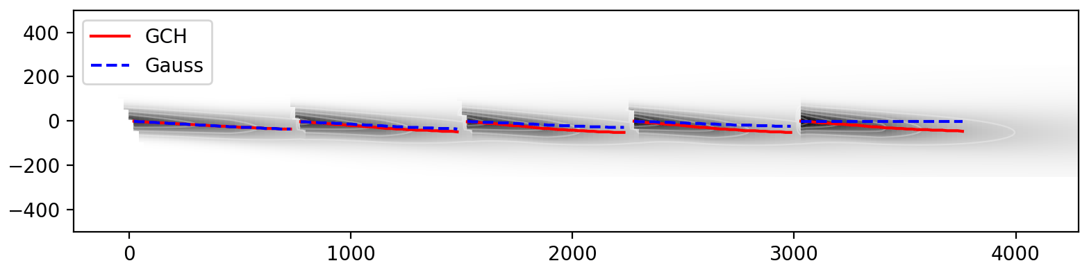
Figure 7Flow field of five turbines using GCH. The resulting centerline behind each turbine is shown for GCH in red and the Gaussian model in blue. The optimized yaw angles are based on the values shown in Table 1.
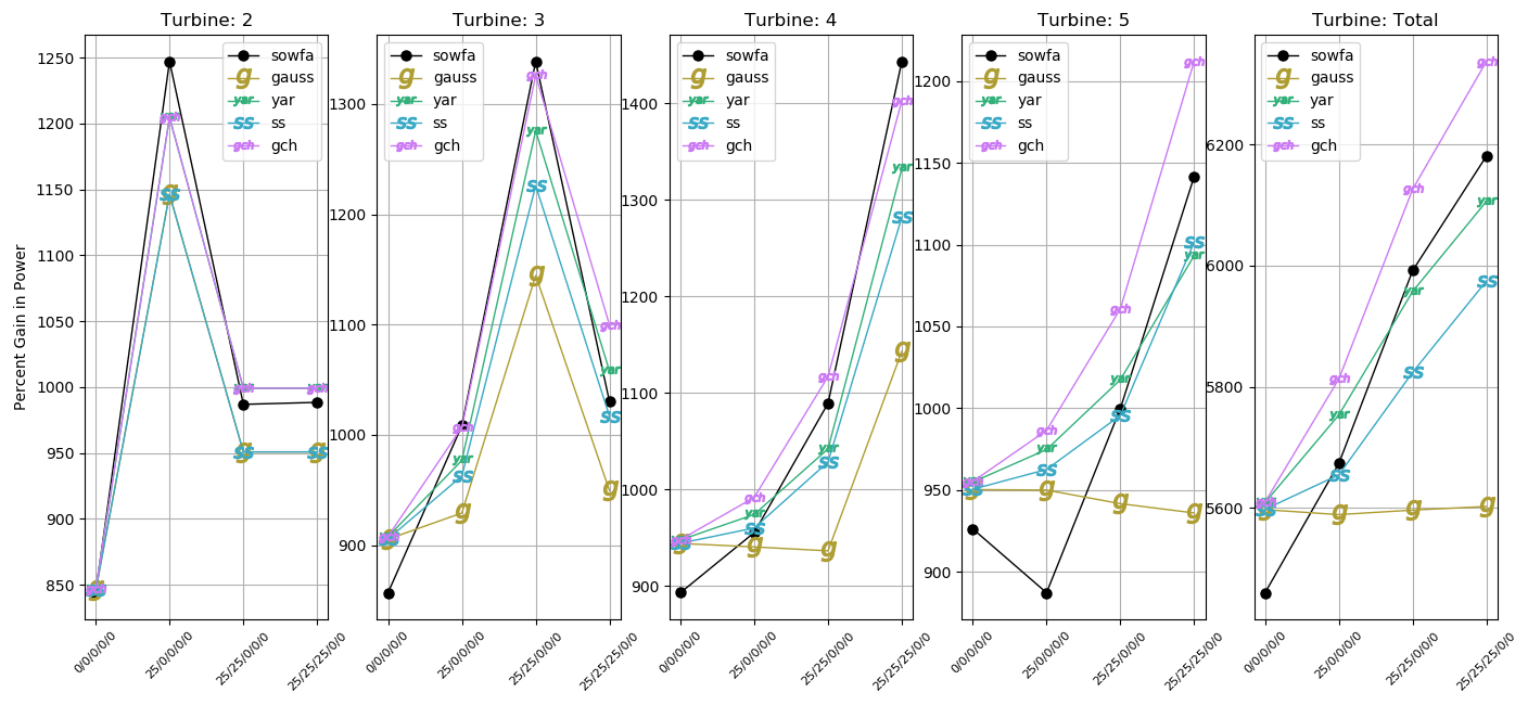
Figure 8Absolute power values for each turbine (excluding the upstream Turbine 1) in the five-turbine array for a wind speed of 8 m/s and low turbulence, i.e., 6 % turbulence intensity. Total turbine power is shown in the rightmost plot. The x axis shows the combination of yaw angles plotted.
Figure 8 shows the absolute powers of each turbine in the five-turbine array, excluding the first turbine, for low-turbulence conditions. The GCH model is able to most closely capture the trends seen in SOWFA, especially when evaluating total turbine power. The power gains for each turbine are shown in Fig. 9. The Gaussian model is pessimistic about the potential gains for the five-turbine case. YAR and SS both contribute significantly to the total gains seen in the five-turbine case. It should be noted that all models have a difficult time predicting the absolute power and the power gain of the last turbine. This may be resolved with a more rigorous turbulence model than the one used in this model; see Annoni et al. (2018). In addition, this model does not directly account for deep array effects, and this may also be a source of error and is a subject of ongoing research.
Figure 10 shows the same five-turbine analysis for the high-turbulence scenario (10 % turbulence intensity). Again, the GCH model most closely follows the trends seen in SOWFA. The most notable difference between GCH and the Gaussian model is that the Gaussian model is extremely pessimistic about wake steering in high turbulence. However, according to SOWFA, large gains are still expected from wake steering even in high turbulence. The GCH model is able to capture the power gains seen in SOWFA at high-turbulence intensities although GCH is still slightly under-predicting the potential gains of wake steering.
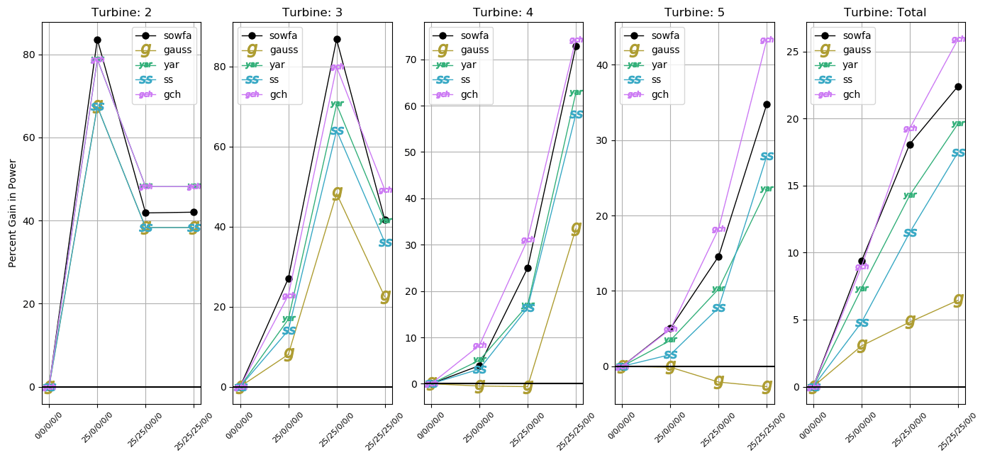
Figure 9Power gains for each turbine (excluding the upstream turbine) in the five-turbine array for a wind speed of 8 m/s and low turbulence, i.e., 6 % turbulence intensity. Total power gain is shown in the rightmost plot. The x axis shows the combination of yaw angles plotted.
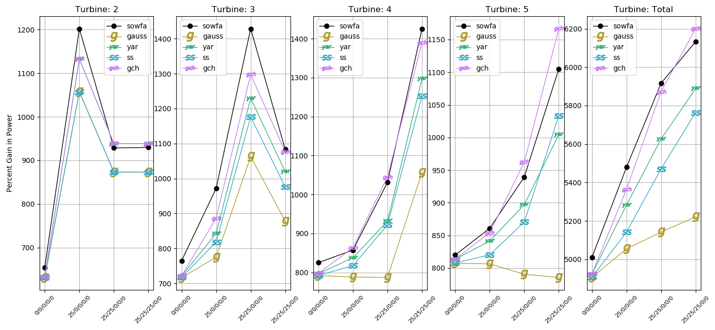
Figure 10Absolute power values for each turbine (excluding the upstream turbine) in the five-turbine array for a wind speed of 8 m/s and high turbulence, i.e., 10 % turbulence intensity. Total turbine power is shown in the rightmost plot. The x axis shows the combination of yaw angles plotted.
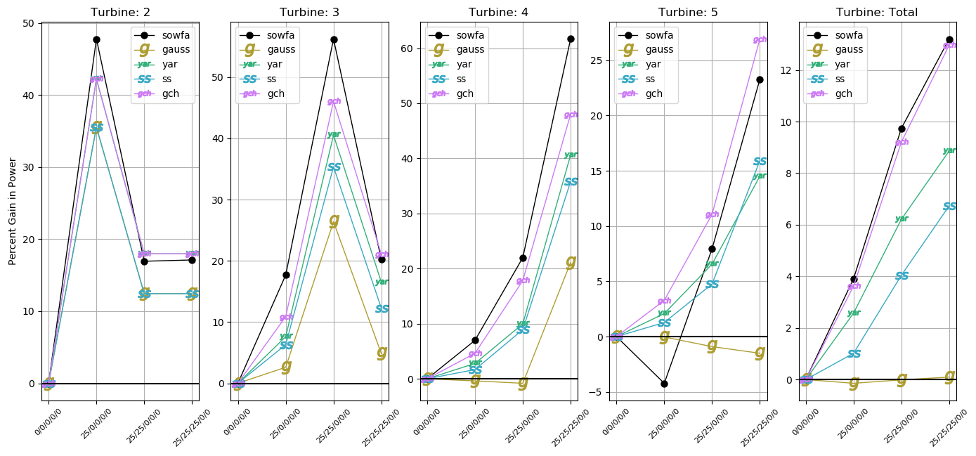
Figure 11Power gains for each turbine (excluding the upstream turbine) in the five-turbine array for a wind speed of 8 m/s and high turbulence, i.e., 10 % turbulence intensity. Total power gain is shown in the rightmost plot. The x axis shows the combination of yaw angles plotted.
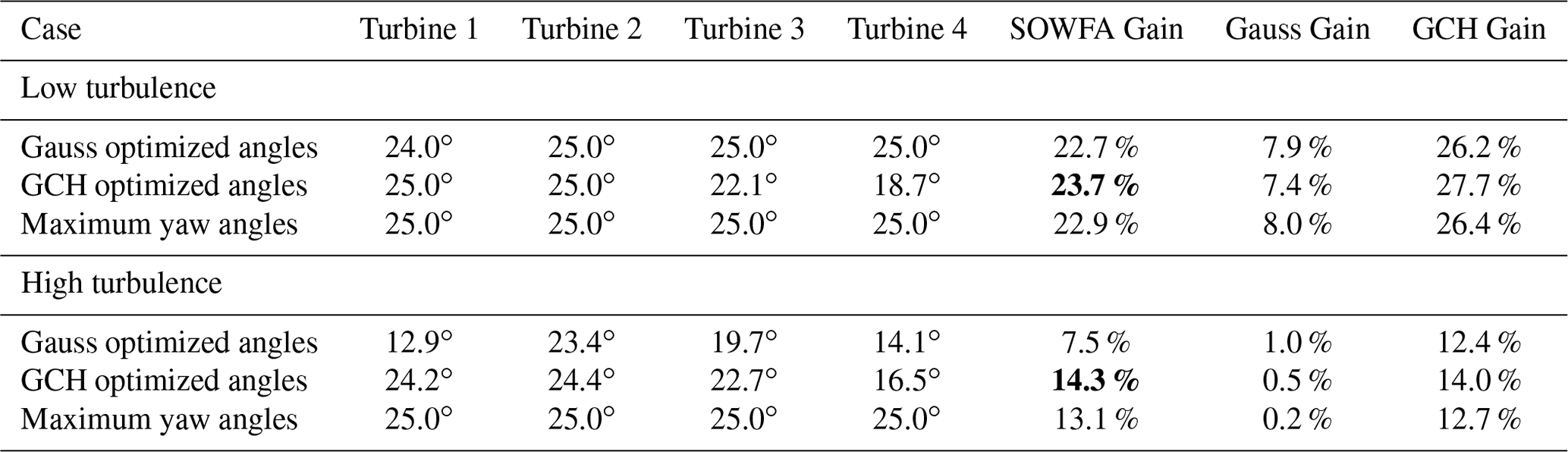
Table 1Five-turbine results for low- and high-turbulence conditions using SOWFA, the Gaussian model, and the GCH model. The bold font indicates the largest power gains identified in SOWFA, which also correspond to yaw angles identified by the GCH model.
Optimization of five-turbine array
Engineering wake models in FLORIS are often used to determine optimal set points for wake steering and assess the performance of these set points. The results of optimizing the Gaussian and GCH models are compared in this section. Specifically, the Gaussian and GCH models were optimized individually for the five-turbine case under low- and high-turbulence conditions. These yaw angles from each optimization were simulated in SOWFA. The power predicted in SOWFA, the Gaussian model, and the GCH model, for each set of yaw angles, are compared in Table 1. The results are compared to (1) a baseline where the yaw angles of all turbines in the five-turbine array are zero and (2) a naive strategy of simply maximizing yaw offsets, subject to an upper bound of 25∘ to limit structural loads, for all turbines except the last.
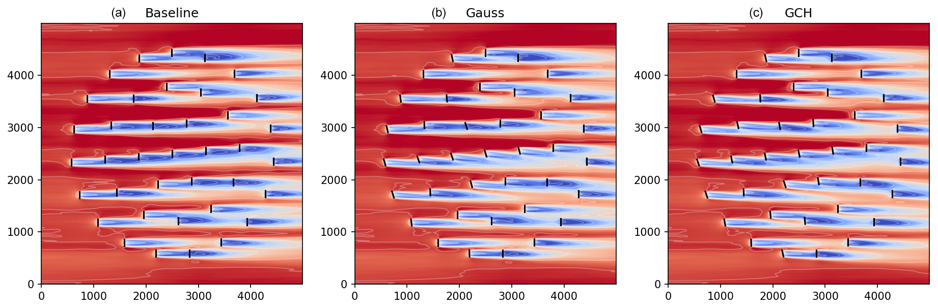
Figure 12Flow field results from SOWFA where the wind direction is 270∘ (Case 2). The left plot shows the baseline case with all turbines aligned with the flow. The middle plot shows the flow field with yaw angles from the optimized Gaussian model, and the right plot shows the flow field with the yaw angles from the optimized GCH model.
In both low- and high-turbulence cases, the GCH optimized yaw angles produced higher power gains in SOWFA compared with the Gaussian model and also outperformed simply operating all turbines (except the last turbine) at a maximum yaw angle of 25∘. Similarly to results observed in a wind tunnel study in Bastankhah and Porté-Agel (2019), GCH produces decreasing yaw angles at farther downstream turbines, indicating that GCH is taking advantage of the effective yaw angle produced by the counter-rotating vortices generated by upstream turbines. Note that GCH more closely predicts the gain observed in SOWFA versus the Gaussian in all cases.
Finally, a full wind farm analysis was performed to quantify the potential of wake steering when effects such as yaw-added recovery and secondary steering are included. For this analysis, we used a 38-turbine wind farm used as in Thomas et al. (2019). The flow field for the baseline case is shown on the left in Fig. 12 where the wind direction is 270∘ and all turbines are aligned with the flow. The middle plot shows the flow field with yaw angles from the optimized Gaussian model, and the right plot shows the flow field with the yaw angles from the optimized GCH model. The analysis was performed for two wind directions, 95 and 270∘, and will be referred to as Case 1 and Case 2 respectively.
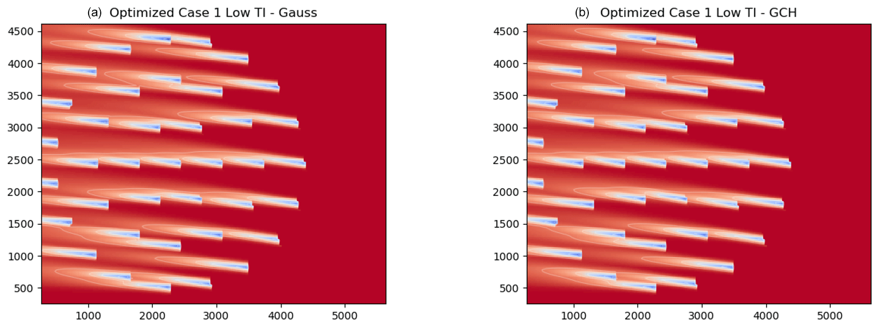
Figure 13Flow fields of the optimized Gaussian model (a) and the optimized GCH model (b) for Case 1 where the wind direction is at 95∘.
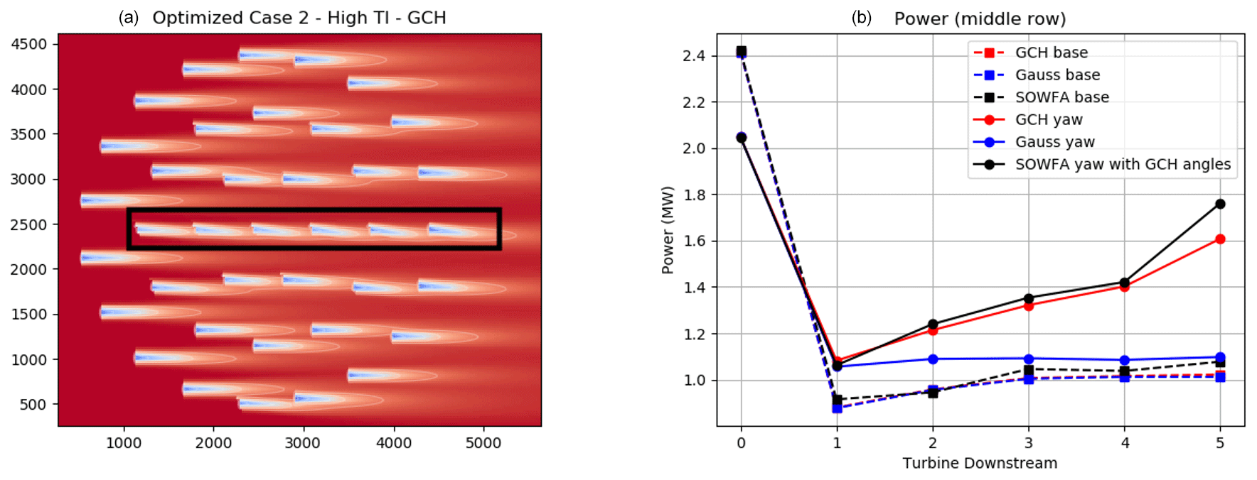
Figure 14Flow field of the optimized GCH model (a) is shown for Case 2, where the wind direction is at 270∘ with a turbulence intensity of 10 %. The power of the centerline of turbines, indicated by the black box, is shown on the right for the Gaussian model, GCH, and SOWFA.
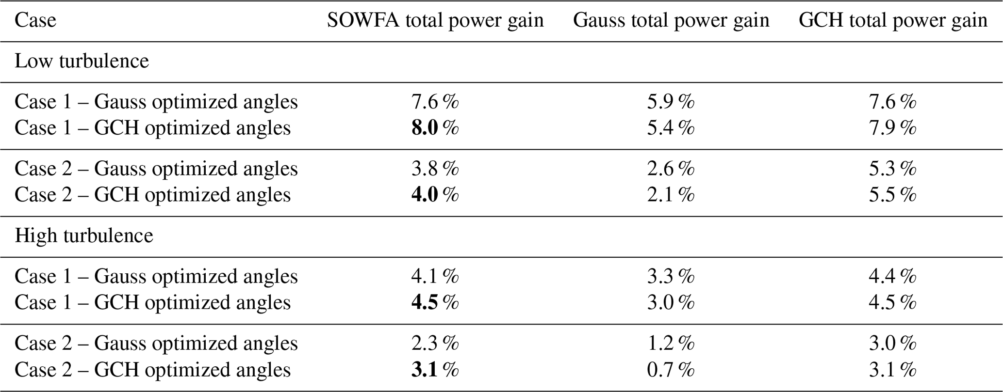
Table 2Wind farm results for low- and high-turbulence conditions for SOWFA, the Gaussian model, and the GCH model. The bold font indicates the largest power gains identified by SOWFA, which also correspond to the yaw angles identified by the GCH model.
Optimizations were performed with the Gaussian model and the GCH model for low (6 %) and high (10 %) turbulence conditions. Flow fields are shown in Fig. 13 for the Gaussian model (left) and the GCH model (right) for Case 1 of 95∘, and Fig. 14 shows the GCH (left) model for Case 2 of 270∘ under low-turbulence conditions and the power of the center line of turbines indicated by the black box in the left figure for SOWFA, the GCH model, and the Gaussian model under baseline and optimized yaw angles. The optimized yaw angles used in Fig. 14 are the optimized yaw angles for the GCH model.
The results of the optimization are shown in Table 2. The optimized yaw angles from the Gaussian model and the GCH model were tested in SOWFA. As with the five-turbine case, the yaw angles produced in the optimization with the GCH model had the largest gain in SOWFA. In addition, the gains computed by the GCH model are closer to the gains in the SOWFA results than the Gaussian model, indicating that the GCH model is better able to capture the secondary effects of the large-scale flow structures generated by misaligned turbines.
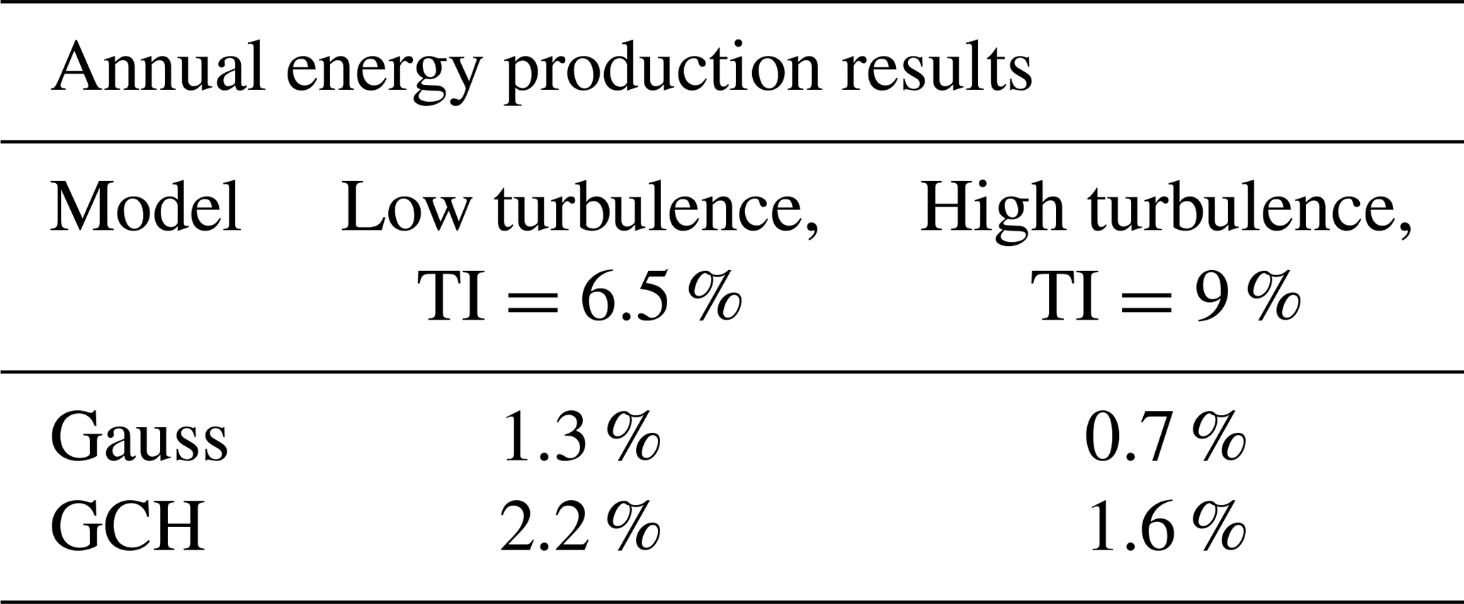
Lastly, a full optimization over a wind rose was run for the wind farm in low- and high-turbulence conditions. The wind rose is shown in Fig. 15 to compute annual energy production (AEP). The Gaussian model and the GCH model were optimized for wake steering over this wind rose, and the AEP gains are reported in Table 3. The Gaussian model predictions of AEP gains are less than half of the gains predicted by the GCH model under both low- and high-turbulence conditions. This is a promising result for understanding the full potential of wake steering in large wind farms. By taking advantage of these large-scale flow structures, there is more potential for increasing the power production in a wind farm, and it is more representative of what is happening within the wind farm as has been shown throughout this paper.
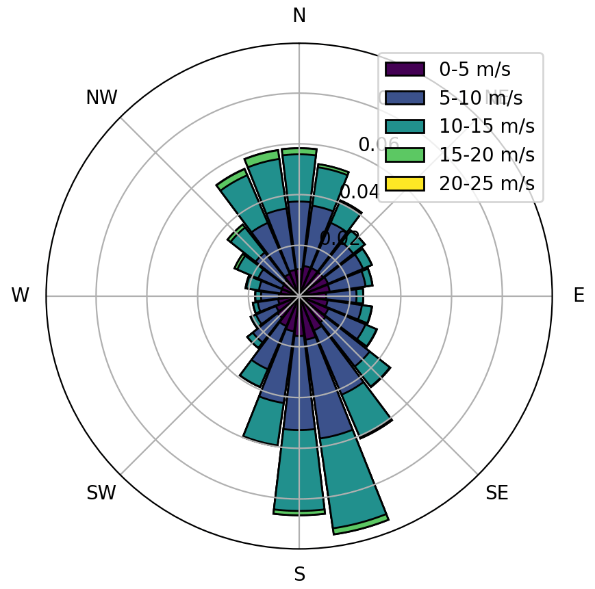
Table 3Wind farm AEP results for low and high turbulence intensity (TI).
This paper introduces an analytical model that better captures the secondary effects of wake steering in a large wind farm. These secondary effects include yaw-added wake recovery as well as secondary wake steering that significantly boosts the impact of wake steering. The results of this model were compared with LES for 3- and 5-turbine arrays as well as a 38-turbine wind farm. The model compared well with results from LES and outperformed the Gaussian model in most cases. Furthermore, this paper demonstrated the possible gains in a large wind farm when considering these large-scale flow structures. Controllers can be developed in the future to manipulate these flow structures to significantly improve the performance of a wind farm.
The code is publicly available and can be accessed on https://github.com/NREL/floris (NREL, 2019).
Please reach out to the authors for access to the data.
JK led the model development and led the writing of the article. PF ran all of the LES cases, led the analysis, and contributed significantly to the text of the article. All authors provided input to this paper.
The authors declare that they have no conflict of interest.
The views expressed in the article do not necessarily represent the views of the DOE or the US Government. The US Government retains and the publisher, by accepting the article for publication, acknowledges that the US Government retains a nonexclusive, paid-up, irrevocable, worldwide license to publish or reproduce the published form of this work, or allow others to do so, for US Government purposes.
This work was authored (in part) by the National Renewable Energy Laboratory, operated by Alliance for Sustainable Energy, LLC, for the U.S. Department of Energy (DOE) under contract no. DE-AC36-08GO28308. Funding was provided by the U.S. Department of Energy Office of Energy Efficiency and Renewable Energy Wind Energy Technologies Office.
This research has been supported by the Department of Energy (contract no. DE-AC36-08GO28308).
This paper was edited by Carlo L. Bottasso and reviewed by Bart M. Doekemeijer and one anonymous referee.
Abkar, M. and Porté-Agel, F.: The effect of atmospheric stability on wind-turbine wakes: A large-eddy simulation study, J. Phys. Conf. Ser., 524, No. 1, IOP Publishing, 2014. a
Abkar, M. and Porté-Agel, F.: Influence of atmospheric stability on wind-turbine wakes: A large-eddy simulation study, Phys. Fluids, 27, 035104, https://doi.org/10.1063/1.4913695, 2015. a, b, c, d
Annoni, J., Fleming, P., Scholbrock, A., Roadman, J., Dana, S., Adcock, C., Porte-Agel, F., Raach, S., Haizmann, F., and Schlipf, D.: Analysis of control-oriented wake modeling tools using lidar field results, Wind Energ. Sci., 3, 819–831, https://doi.org/10.5194/wes-3-819-2018, 2018. a, b
Annoni, J., Dall'Anese, E., Hong, M., and Bay, C. J.: Efficient Distributed Optimization of Wind Farms Using Proximal Primal-Dual Algorithms, in: Proceedings of the 2019 American Control Conference (ACC), American Control Conference (ACC) IEEE, July 2019, Philadelphia, PA, 4173–4178, 2019. a
Bastankhah, M. and Porté-Agel, F.: A new analytical model for wind-turbine wakes, Renew. Energ., 70, 116–123, 2014. a, b, c
Bastankhah, M. and Porté-Agel, F.: Experimental and theoretical study of wind turbine wakes in yawed conditions, J. Fluid Mech., 806, 506–541, 2016. a, b, c, d, e, f, g, h, i, j
Bastankhah, M. and Porté-Agel, F.: Wind farm power optimization via yaw angle control: A wind tunnel study, J. Renew. Sustain. Ener., 11, 023301, https://doi.org/10.1063/1.5077038, 2019. a, b
Bay, C. J., Annoni, J., Martínez-Tossas, L. A., Pao, L. Y., and Johnson, K. E.: Flow Control Leveraging Downwind Rotors for Improved Wind Power Plant Operation, in: Proceedings of the 2019 American Control Conference (ACC), Philadelphia, PA, July 2019, 2843–2848, 2019. a, b, c
Churchfield, M. J., Lundquist, J. K., Quon, E., Lee, S., and Clifton, A.: Large-Eddy Simulations of Wind Turbine Wakes Subject to Different Atmospheric Stabilities, in: American Geophysical Union Fall Meeting, San Francisco, CA, December 2014, vol. 2014, A11G-3085, 2014. a
Ciri, U., Rotea, M. A., and Leonardi, S.: Effect of the turbine scale on yaw control, Wind Energy, 21, 1395–1405, 2018. a
Crespo, A., Hernández, J., and Frandsen, S.: Survey of modelling methods for wind turbine wakes and wind farms, Wind Energy, 2, 1–24, 1999. a, b
Fleming, P., Aho, J., Gebraad, P., Pao, L., and Zhang, Y.: CFD Simulation Study of Active Power Control in Wind Plants, in: American Control Conference (ACC) IEEE, Boston, MA, July 2016, 1413–1420, 2016. a
Fleming, P., Annoni, J., Churchfield, M., Martinez-Tossas, L. A., Gruchalla, K., Lawson, M., and Moriarty, P.: A simulation study demonstrating the importance of large-scale trailing vortices in wake steering, Wind Energ. Sci., 3, 243–255, https://doi.org/10.5194/wes-3-243-2018, 2018a. a, b, c, d
Fleming, P., Annoni, J., Martínez-Tossas, L. A., Raach, S., Gruchalla, K., Scholbrock, A., Churchfield, M., and Roadman, J.: Investigation into the shape of a wake of a yawed full-scale turbine, J. Phys. Conf. Ser., 1037, 032010, IOP Publishing, 2018b. a
Fleming, P., King, J., Dykes, K., Simley, E., Roadman, J., Scholbrock, A., Murphy, P., Lundquist, J. K., Moriarty, P., Fleming, K., van Dam, J., Bay, C., Mudafort, R., Lopez, H., Skopek, J., Scott, M., Ryan, B., Guernsey, C., and Brake, D.: Initial results from a field campaign of wake steering applied at a commercial wind farm – Part 1, Wind Energ. Sci., 4, 273–285, https://doi.org/10.5194/wes-4-273-2019, 2019. a, b
Fleming, P., King, J., Simley, E., Roadman, J., Scholbrock, A., Murphy, P., Lundquist, J. K., Moriarty, P., Fleming, K., van Dam, J., Bay, C., Mudafort, R., Jager, D., Skopek, J., Scott, M., Ryan, B., Guernsey, C., and Brake, D.: Continued results from a field campaign of wake steering applied at a commercial wind farm – Part 2, Wind Energ. Sci., 5, 945–958, https://doi.org/10.5194/wes-5-945-2020, 2020. a
Gebraad, P., Teeuwisse, F., Wingerden, J., Fleming, P. A., Ruben, S., Marden, J., and Pao, L.: Wind plant power optimization through yaw control using a parametric model for wake effects – a CFD simulation study, Wind Energy, 19, 95–114, 2016. a, b
Gebraad, P., Thomas, J. J., Ning, A., Fleming, P., and Dykes, K.: Maximization of the annual energy production of wind power plants by optimization of layout and yaw-based wake control, Wind Energy, 20, 97–107, 2017. a
Howland, M. F., Bossuyt, J., Martínez-Tossas, L. A., Meyers, J., and Meneveau, C.: Wake structure in actuator disk models of wind turbines in yaw under uniform inflow conditions, J. Renew. Sustain. Ener., 8, 043301, https://doi.org/10.1063/1.4955091, 2016. a, b
Jensen, N. O.: A note on wind generator interaction, Technical Report Risø-M-2411, Risø National Laboratory, Frederiksborgvej 399, 4000 Roskilde, Denmark, 17 pp., 1984. a
Jiménez, Á., Crespo, A., and Migoya, E.: Application of a LES technique to characterize the wake deflection of a wind turbine in yaw, Wind Energy, 13, 559–572, 2010. a
Katić, I., Højstrup, J., and Jensen, N. O.: A simple model for cluster efficiency, in: European wind energy association conference and exhibition, Rome, Italy, 1, 407–410, 1986. a
Martínez-Tossas, L. A., Churchfield, M. J., and Leonardi, S.: Large eddy simulations of the flow past wind turbines: actuator line and disk modeling, Wind Energy, 18, 1047–1060, 2015. a
Martínez-Tossas, L. A., Annoni, J., Fleming, P. A., and Churchfield, M. J.: The aerodynamics of the curled wake: a simplified model in view of flow control, Wind Energ. Sci., 4, 127–138, https://doi.org/10.5194/wes-4-127-2019, 2019. a, b, c, d, e, f, g, h, i
Medici, D. and Alfredsson, P.: Measurements on a wind turbine wake: 3D effects and bluff body vortex shedding, Wind Energy, 9, 219–236, 2006. a, b
Niayifar, A. and Porté-Agel, F.: A new analytical model for wind farm power prediction, J. Phys., 625, 012039, https://doi.org/10.1088/1742-6596/625/1/012039, 2015. a, b, c, d, e, f, g, h, i
NREL: FLORIS. Version 1.1.4, available at: https://github.com/NREL/floris (last access: December 2020), 2019. a, b
Pope, S. B.: Turbulent flows, Cambridge University Press, ISBN 9780511840531, https://doi.org/10.1017/CBO9780511840531, 2000. a, b, c
Schottler, J., Hölling, A., Peinke, J., and Hölling, M.: Wind tunnel tests on controllable model wind turbines in yaw, in: Proceedings of the 34th Wind Energy Symposium, San Diego, CA, January 2016, 1523, 2016. a
Shapiro, C. R., Gayme, D. F., and Meneveau, C.: Modelling yawed wind turbine wakes: a lifting line approach, J. Fluid Mech., 841, R1, https://doi.org/10.1017/jfm.2018.75, 2018. a
Simley, E., Fleming, P., and King, J.: Design and analysis of a wake steering controller with wind direction variability, Wind Energ. Sci., 5, 451–468, https://doi.org/10.5194/wes-5-451-2020, 2020. a, b
Stanley, A. P. J. and Ning, A.: Massive simplification of the wind farm layout optimization problem, Wind Energ. Sci., 4, 663–676, https://doi.org/10.5194/wes-4-663-2019, 2019. a, b
Stull, R. B.: An introduction to boundary layer meteorology, Springer Science and Business Media, Germany, 2012. a, b
Thomas, J. J., Annoni, J., Fleming, P. A., and Ning, A.: Comparison of Wind Farm Layout Optimization Results Using a Simple Wake Model and Gradient-Based Optimization to Large Eddy Simulations, AIAA Scitech 2019 Forum, San Diego, CA, January 2019, 0538, 2019. a
Vollmer, L., Steinfeld, G., Heinemann, D., and Kühn, M.: Estimating the wake deflection downstream of a wind turbine in different atmospheric stabilities: an LES study, Wind Energ. Sci., 1, 129–141, https://doi.org/10.5194/wes-1-129-2016, 2016. a, b
Wagenaar, J., Machielse, L., and Schepers, J.: Controlling wind in ECN’s scaled wind farm, in: Proceedings of the Europe Premier Wind Energy Event, Copenhagen, DK, April 2012, 685–694, 2012. a