A method for preliminary rotor design – Part 2: Wind turbine Optimization with Radial Independence

A novel wind turbine rotor optimization methodology is presented. Using an assumption of radial independence it is possible to obtain an optimal relationship between the global power (C_P) and load coefficient (C_T, C_FM) through the use of Karush–Kuhn–Tucker (KKT) multipliers, leaving an optimization problem that can be solved at each radial station independently. It allows solving load constraint power and annual energy production (AEP) optimization problems where the optimization variables are only the KKT multipliers (scalars), one for each of the constraints. For the paper, two constraints, namely the thrust and blade root flap moment, are used, leading to two optimization variables.

Applying the optimization methodology to maximize power (P) or annual energy production (AEP) for a given thrust and blade root flap moment, but without a cost function, leads to the same overall result with the global optimum being unbounded in terms of rotor radius ($\stackrel{\mathrm{̃}}{R}$) with a global optimum being at $\stackrel{\mathrm{̃}}{R}\to \mathrm{\infty }$. The increase in power and AEP is in this case ΔP=50 % and ΔAEP=70 %, with a baseline being the Betz optimum rotor.

With a simple cost function and with the same setup of the problem, a power-per-cost (PpC) optimization resulted in a power-per-cost increase of ΔPpC=4.2 % with a radius increase of ΔR=7.9 % as well as a power increase of ΔP=9.1 %. This was obtained while keeping the same flap moment and reaching a lower thrust of $\mathrm{\Delta }T=-\mathrm{3.8}$ %. The equivalent for AEP-per-cost (AEPpC) optimization leads to increased cost efficiency of ΔAEPpC=2.9 % with a radius increase of ΔR=17 % and an AEP increase of ΔAEP=13 %, again with the same, maximum flap moment, while the maximum thrust is −9.0 % lower than the baseline.

1 Introduction

Wind turbine design optimization has been an integral part of wind turbine design since the start of the wind turbine industry. The target for such optimization has varied greatly from pure aerodynamic optimization with the target to maximize the power extraction (see Manwell et al., 2010, Sørensen, 2016 and Jamieson, 2018) to a more holistic turbine design where the target is to minimize the cost of the turbine through modeling the physics of the turbine components as well as their associated cost; see, e.g., Fuglsang et al. (2002), Hjort et al. (2009), Bottasso et al. (2012), Dykes and Meadows (2012), and Perez-Moreno et al. (2016). Common to these approaches the connection of a set of simulation tools (e.g., BEM solver, structural solver, controller) through a cost function, leading to a fairly complicated optimization problem with a lot of design variables. As a consequence, the computational time for each evaluation of the objective function might be unfeasible for exploring the design space and carrying out sensitivity studies considering the number of design variables. Exploring the design space is especially important for the preliminary design phase where, e.g., the rotor size and rated power need to be determined.

Lately, some research has been performed within preliminary rotor design which seems to have started with the concept of low-induction rotors (Chaviaropoulos and Voutsinas, 2012) where they investigate the optimal constant axial induction (a) with a flap moment constraint, arriving at an optimum of a=0.2. A similar study was performed by Buck and Garvey (2015b) where they used a cost function to find the most cost-effective rotor to have a=0.25. They also performed a study (Buck and Garvey, 2015a) where they investigated so-called thrust clipping (limiting the maximum thrust) as a means to find the optimal cost-effective rotor. This author recently performed a study (Loenbaek et al., 2020) where the approach taken by Chaviaropoulos and Voutsinas (2012) was generalized to include additional constraints (e.g., tip deflection as well as constant mass). This study investigated the impact on the power curve, where thrust clipping is found to be the design concept that leads to the largest energy increase, as compared to the low-induction rotor design concept.

Common to these studies is the assumption of constant axial induction along the rotor span. There have also been some studies to investigate the impact of allowing the axial induction to change along the rotor span. Kelley (2017) investigates the optimal distribution of a, showing that when keeping a fixed maximum bending moment the optimal a distribution tapers towards the tip of the blade. Recently a study by Jamieson (2020) extended the work of Chaviaropoulos and Voutsinas (2012) where they allow for variations in a along the span, showing that it is possible to reach the same power increase, but with a smaller radius increase. They also see a similar tapering a distribution towards the tip as Kelley (2017). The current study builds on top of this works, and it could be seen as an extension of previous work by this author (Loenbaek et al., 2020), where a variation in a (or loading) along the rotor span is added, as well as including a simple cost function. The developed optimization methodology described in this paper is Part 2 of a two-part paper, where Part 1 (Loenbaek et al., 2021) describes the aerodynamic model used thought out this paper.

In this paper, an optimization methodology is presented which aims to maximize the power (P) or annual energy production (AEP) with a fixed radius increase. Since the pure aerodynamic optimization leads to an unbounded optimum, a simple cost function is introduced, leading to power-per-cost (PpC) and AEP-per-cost optimization. The aerodynamic and cost modeling is kept at a fairly simple level with BEM-like aerodynamics and simple radius-dependent cost functions. It allows for the optimization problem to be solved for the global optimum within numerical accuracy. The crucial assumption made for this to be possible is the assumption of radial independence which allows the optimization problem to be made into a set of nested optimizations, each resulting in a well-behaved optimization problem. A key innovation is that the optimization is based on loading and not the design variables (e.g., control points for chord and twist), which leads to a large reduction in the number of design variables and a simplification of the optimization problem. Thus, in contrast to many methods used to optimize wind turbine rotors, this method is very simple. Even though it is simple it is thought to be an important step for preliminary rotor design where one would like to investigate the impact of changes in the cost function or constraints. This is especially important where technology improvements should be targeted in order to lead to the biggest improvements in PpC or AEPpC.

This paper is split into two sections: the “Optimization methodology” section, where the optimization problem is presented and the process of solving the optimization problem with the assumption of radial independence is then given; and then the “Results and discussion” section, where the results from solving the optimization problem are presented and discussed.

2 Optimization methodology

In this section, we will present an optimization methodology for wind turbine rotor optimization. It is named Wind turbine Optimization with Radial Independence (WOwRI). Before presenting WOwRI a discussion of the assumptions as well as the terminology is given, ending with a short discussion of the aerodynamic solver used. Then WOwRI is presented for power optimization with a fixed radius increase as well as wind speed. WOwRI is then extended for AEP optimization with a fixed radius increase, and at last WOwRI is extended for optimization with a simple cost function to determine optimal rotor size.

The core assumption for WOwRI is the assumption of radial independence. An important concept in this relation is the difference between global and local variables. Global rotor variables have a scalar value for the whole rotor (e.g., power, thrust), whereas local rotor variables have a scalar at a given rotor radius (r) location (e.g., lift, drag). With this definition, the assumption of radial independence is applied for the local rotor variables, meaning that changes in the loading (like lift) at one radial location will not affect the flow state (flow through the rotor plane) at any other radial location. This is the same assumption made for blade element momentum theory (Sørensen, 2016, p. 99).

An assumption that is related to the radial independence is a direct relationship between the local thrust loading and the local power at the same radial location. It means that if the local thrust loading is given the local power can be computed. This is further discussed in Sect. 2.1.

Throughout this paper, the flow is assumed to be steady state. As a consequence, when the optimization is made with load constraints (e.g., thrust and flap moment), it is the steady-state load that is constrained. But for the current utility scale wind turbine design, it is common that the design is driven by the dynamic extreme loads. It means that the underlying assumption for this optimization methodology is that a constraint steady-state load is in some way connected with the dynamic extreme load. This assumption is, however, not tested in this paper.

WOwRI is based on power (P) optimization with a given set of load constraints. These constraints can be (but are not limited to) thrust, flap moment, tip deflection, and max stress/strain, where the key requirement for the constraint to be suited for WOwRI is that it satisfies the radial independence requirement. A form that satisfied (but is not limited to) this requirement is

$$\begin{array}{}\text{(1)}& X_{\mathrm{con}}=\underset{\mathrm{0}}{\overset{R}{\int }}{\displaystyle \frac{\partial T}{\partial r}}\left(r\right)\cdot f_X\left(r\right)\mathrm{d}r,\end{array}$$

where X_con is a global rotor variable (like thrust, T), $\frac{\partial T}{\partial r}\left(r\right)$ is the thrust loading density (loading per meter) and f_X(r) is a function that changes the impact of thrust loading density at each radial station. This is a rather abstract definition, but showing how an extensive list of constraints is related to this definition is though to be outside the scope of this paper since the purpose is to present the optimization methodology. Instead, the focus will be on two specific constraints, namely thrust (T) and blade root flap bending moment (M_f) constraints. These two constraints are given as

$$\begin{array}{}\text{(2)}& {\displaystyle }& {\displaystyle }T=\underset{\mathrm{0}}{\overset{R}{\int }}{\displaystyle \frac{\partial T}{\partial r}}\mathrm{d}r\left(\mathrm{thrust}\mathrm{constraint},\mathrm{with}:f_X=\mathrm{1}\right),\text{(3)}& {\displaystyle }& {\displaystyle }{M}_{\mathrm{f}}=\underset{\mathrm{0}}{\overset{R}{\int }}{\displaystyle \frac{\partial T}{\partial r}}r\mathrm{d}r\left(\mathrm{flap}\text{-}\mathrm{moment}\mathrm{constraint},\mathrm{with}:f_X=r\right),\end{array}$$

where the relationship with the generalized constraint form shown in Eq. (1) is given in parentheses.

2.1 The aerodynamic solver

The aerodynamic solver (Radially Independent Actuator Disc model – RIAD) used though out this paper is further described in Part 1, and therefore only a brief overview is given here. It makes an explicit relationship between the local-thrust coefficient (C_LT – normalized $\partial T/\partial r$) and the local-power coefficient (C_LP – normalized $\partial P/\partial r$) with given operational conditions such as the global tip speed ratio (λ) and the local glide ratio ($C_{\mathrm{l}}/C_{\mathrm{d}}$) and may include tip loss as well. A diagram showing the relationship graphically can be seen in Fig. 1

Figure 1 Diagram showing a diagram for the Radially Independent Actuator Disc (RIAD) model.

2.2 Power optimization

In this section, the optimization methodology that allows for the fast and very efficient solution to the optimization is derived. It finds the optimal power for a fixed rotor increase. In principle, the rotor radius could also be an optimization parameter, but as is shown later, the optimal global power turns out to be unbounded, and having the solution for the fixed rotor radius increase allows for optimization with a simple cost function, which is further explained later. The main outcome of this section is a function that through solving an optimization problem gives the optimal power for a given set of constraints with a fixed radius increase and fixed wind speed (P_opt(R, V)).

2.2.1 Problem formulation

The optimization problem is maximizing power (P) with two constraints, the maximum allowable thrust (T₀) and a maximum allowable blade root flap bending moment (M_f) for a fixed rotor radius and fixed wind speed. The design variable is the distributed thrust loading along the span of the rotor $\left(\frac{\partial \mathit{T}}{\partial \mathit{r}}\left(r\right)\right)$. It is important to note that the distributed load is a function of r or when discretized a vector.

Mathematically the problem can be stated as

$$\begin{array}{}\text{(4)}& \begin{array}{rl}& \underset{{\displaystyle \frac{\partial \mathit{T}}{\partial \mathit{r}}}}{\max }P\left({\displaystyle \frac{\partial \mathit{T}}{\partial \mathit{r}}}\right)\\ & \mathrm{subj}.\begin{array}{ll}T\left(\frac{\partial \mathit{T}}{\partial \mathit{r}}\right)& \le T_{\mathrm{0}}\\ M_{\mathrm{f}}\left(\frac{\partial \mathit{T}}{\partial \mathit{r}}\right)& \le M_{\mathrm{f},\mathrm{0}}\end{array},\end{array}\end{array}$$

where the boldface $\frac{\partial \mathit{T}}{\partial \mathit{r}}$ signifies that it is a function and not just a scalar. The zero subscript denotes a constraint limit.

2.2.2 Problem formulation in integral form and normalization

Using the same normalization as in Part 1 (Loenbaek et al., 2021, Sect. 2.1, Eqs. 3–6) the power and constraints can be normalized as

$$\begin{array}{}\text{(5)}& {\displaystyle }& {\displaystyle }\stackrel{\mathrm{̃}}{P}={\stackrel{\mathrm{̃}}{R}}^{\mathrm{2}}{\stackrel{\mathrm{̃}}{V}}^{\mathrm{3}}{C}_{\mathrm{P}}={\stackrel{\mathrm{̃}}{R}}^{\mathrm{2}}{\stackrel{\mathrm{̃}}{V}}^{\mathrm{3}}\mathrm{2}\underset{\mathrm{0}}{\overset{\mathrm{1}}{\int }}{C}_{\mathrm{LP}}\left(C_{\mathrm{LT}}\left(\stackrel{\mathrm{̃}}{r}\right)\right)\cdot \stackrel{\mathrm{̃}}{r}\mathrm{d}\stackrel{\mathrm{̃}}{r},\text{(6)}& {\displaystyle }& {\displaystyle }\stackrel{\mathrm{̃}}{T}={\stackrel{\mathrm{̃}}{R}}^{\mathrm{2}}{\stackrel{\mathrm{̃}}{V}}^{\mathrm{2}}{C}_{\mathrm{T}}={\stackrel{\mathrm{̃}}{R}}^{\mathrm{2}}{\stackrel{\mathrm{̃}}{V}}^{\mathrm{2}}\mathrm{2}\underset{\mathrm{0}}{\overset{\mathrm{1}}{\int }}{C}_{\mathrm{LT}}\left(\stackrel{\mathrm{̃}}{r}\right)\cdot \stackrel{\mathrm{̃}}{r}\mathrm{d}\stackrel{\mathrm{̃}}{r},\end{array}$$

$$\begin{array}{}\text{(7)}& {\stackrel{\mathrm{̃}}{M}}_{\mathrm{f}}={\stackrel{\mathrm{̃}}{R}}^{\mathrm{3}}{\stackrel{\mathrm{̃}}{V}}^{\mathrm{2}}{C}_{\mathrm{FM}}={\stackrel{\mathrm{̃}}{R}}^{\mathrm{3}}{\stackrel{\mathrm{̃}}{V}}^{\mathrm{2}}\mathrm{3}\underset{\mathrm{0}}{\overset{\mathrm{1}}{\int }}{C}_{\mathrm{LT}}\left(\stackrel{\mathrm{̃}}{r}\right)\cdot {\stackrel{\mathrm{̃}}{r}}^{\mathrm{2}}\mathrm{d}\stackrel{\mathrm{̃}}{r},\end{array}$$

where $\stackrel{\mathrm{̃}}{R}=\frac{R}{R_{\mathrm{0}}}$ and $\stackrel{\mathrm{̃}}{V}=V/V_{\mathrm{rated},\mathrm{0}}$, with R₀ being a reference radius and V_rated,0 the rated wind speed for a reference turbine. Both are related to the constraint limit. The optimization problem can therefore be reformulated as

$$\begin{array}{}\text{(8)}& \begin{array}{rl}& \underset{{\mathit{C}}_{\mathrm{LT}}}{\max }{C}_{\mathrm{P}}\left({\mathit{C}}_{\mathrm{LT}}\right)\cdot {\stackrel{\mathrm{̃}}{R}}^{\mathrm{2}}{\stackrel{\mathrm{̃}}{V}}^{\mathrm{3}}\\ & \text{subj.}\begin{array}{ll}{C}_{\mathrm{T}}\left({\mathit{C}}_{\mathrm{LT}}\right)\cdot {\stackrel{\mathrm{̃}}{R}}^{\mathrm{2}}{\stackrel{\mathrm{̃}}{V}}^{\mathrm{2}}& \le {\stackrel{\mathrm{̃}}{T}}_{\mathrm{0}}\\ C_{\mathrm{FM}}\left({\mathit{C}}_{\mathrm{LT}}\right)\cdot {\stackrel{\mathrm{̃}}{R}}^{\mathrm{3}}{\stackrel{\mathrm{̃}}{V}}^{\mathrm{2}}& \le {\stackrel{\mathrm{̃}}{M}}_{\mathrm{f},\mathrm{0}}\end{array}.\end{array}\end{array}$$

2.2.3 Reformulating as a Lagrange objective function

The optimization problem stated in the previous sections has a solution that needs to satisfy the Karush–Kuhn–Tucker (KKT) (Kuhn and Tucker, 1951) theorem to be optimal. It means that a solution to the original problem can also be found by solving the optimization problem in Eq. (9), where the objective function has been reformulated as a Lagrange objective function (ℒ^*) (including the constraints in the objective function):

$$\begin{array}{}\text{(9)}& \begin{array}{rl}\underset{{\mathit{C}}_{\mathrm{LT}},W_{\mathrm{0}}^{*},W_{\mathrm{1}}^{*}}{\max }{\mathcal{L}}^{*}& =\underset{{\mathit{C}}_{\mathrm{LT}},W_{\mathrm{0}}^{*},W_{\mathrm{1}}^{*}}{\max }\left[C_{\mathrm{P}}\left({\mathit{C}}_{\mathrm{LT}}\right)\cdot {\stackrel{\mathrm{̃}}{R}}^{\mathrm{2}}{\stackrel{\mathrm{̃}}{V}}^{\mathrm{3}}\right.\\ & -W_{\mathrm{0}}^{*}\left[C_{\mathrm{T}}\left({\mathit{C}}_{\mathrm{LT}}\right)\cdot {\stackrel{\mathrm{̃}}{R}}^{\mathrm{2}}{\stackrel{\mathrm{̃}}{V}}^{\mathrm{2}}-{\stackrel{\mathrm{̃}}{T}}_{\mathrm{0}}\right]\\ & \left.-W_{\mathrm{1}}^{*}\left[C_{\mathrm{FM}}\left({\mathit{C}}_{\mathrm{LT}}\right)\cdot {\stackrel{\mathrm{̃}}{R}}^{\mathrm{3}}{\stackrel{\mathrm{̃}}{V}}^{\mathrm{2}}-{\stackrel{\mathrm{̃}}{M}}_{\mathrm{f},\mathrm{0}}\right]\right],\end{array}\end{array}$$

where $W_i^{*}$'s are the so-called KKT multipliers with the property $W_i^{*}\ge \mathrm{0}$. These $W_i^{*}$'s need to be adjusted for active constraints until the constraint is met. For an inactive constraint $W_i^{*}=\mathrm{0}$.

The key point for rewriting the optimization as a Lagrange objective function is to be able to solve the optimization of the C_LT distribution. To do this we will look at the case where $W_{\mathrm{0}}^{*}$ and $W_{\mathrm{1}}^{*}$ are constant input parameters. Since the location of the optimum dose not change with scaling and a constant offset, a new Lagrange objective function can be written as

$$\begin{array}{}\text{(10)}& \begin{array}{rl}\underset{{\mathit{C}}_{\mathrm{LT}}}{\max }\mathcal{L}& =\underset{{\mathit{C}}_{\mathrm{LT}}}{\max }\left[C_{\mathrm{P}}\left({\mathit{C}}_{\mathrm{LT}}\right)-W_{\mathrm{0}}{C}_{\mathrm{T}}\left({\mathit{C}}_{\mathrm{LT}}\right)\right.\\ & \left.-W_{\mathrm{1}}{C}_{\mathrm{FM}}\left({\mathit{C}}_{\mathrm{LT}}\right)\right],\end{array}\end{array}$$

where scaling in front of C_T and C_FM has be absorbed into W₀ and W₁ respectively (note the change from $W_i^{*}$ to W_i to stress that they have been rescaled between Eqs. 9 and 10). Any solution for the scaled Lagrange function (Eq. 10) (in terms of C_LT) will also be a solution to the non-scaled Lagrange function (Eq. 9) and here a solution for the optimization problem (Eq. 8) for some set of constraint limits. But which set of constraints is not known prior to solving the optimization problem. Equation (10) is also sometimes referred to as the Pareto-optimal problem for C_P, C_T and C_FM, giving the maximum C_P for a given value of C_T, C_FM or any combination of the two. By varying the W_i's the location on the so-called Pareto-optimal surface is changed.

2.2.4 Solving for the optimal loading distribution

In this section we will apply the assumption of radial independence to show that the optimal solution for the trade-off between global power (C_P) and the loading (C_T, C_FM) can be found for each radial station independently. In integral form the optimization for the optimal loading reads

$$\begin{array}{}\text{(11)}& \begin{array}{rl}\underset{{\mathit{C}}_{\mathrm{LT}}}{\max }\mathcal{L}& =\underset{{\mathit{C}}_{\mathrm{LT}}}{\max }\left[\mathrm{2}\underset{\mathrm{0}}{\overset{\mathrm{1}}{\int }}{C}_{\mathrm{LP}}\left(C_{\mathrm{LT}}\left(r\right)\right)\cdot \stackrel{\mathrm{̃}}{r}\mathrm{d}\stackrel{\mathrm{̃}}{r}\right.\\ & -W_{\mathrm{0}}\mathrm{2}\underset{\mathrm{0}}{\overset{\mathrm{1}}{\int }}{C}_{\mathrm{LT}}\left(r\right)\cdot \stackrel{\mathrm{̃}}{r}\mathrm{d}\stackrel{\mathrm{̃}}{r}-W_{\mathrm{1}}\mathrm{3}\underset{\mathrm{0}}{\overset{\mathrm{1}}{\int }}{C}_{\mathrm{LT}}\left(r\right)\\ & \left.\cdot {\stackrel{\mathrm{̃}}{r}}^{\mathrm{2}}\mathrm{d}\stackrel{\mathrm{̃}}{r}\right].\end{array}\end{array}$$

The three integrations can be combined into one since W_i is independent of $\stackrel{\mathrm{̃}}{r}$. Then applying the radial independence the maximization can be moved within the integration:

$$\begin{array}{}\text{(12)}& \begin{array}{rl}\underset{{\mathit{C}}_{\mathrm{LT}}}{\max }\mathcal{L}& =\underset{\mathrm{0}}{\overset{\mathrm{1}}{\int }}\underset{{\mathit{C}}_{\mathrm{LT}}}{\max }\left[\mathrm{2}{C}_{\mathrm{LP}}\left(C_{\mathrm{LT}}\right)\stackrel{\mathrm{̃}}{r}-\mathrm{2}{W}_{\mathrm{0}}{C}_{\mathrm{LT}}\stackrel{\mathrm{̃}}{r}\right.\\ & \left.-\mathrm{3}{W}_{\mathrm{1}}{C}_{\mathrm{LT}}{\stackrel{\mathrm{̃}}{r}}^{\mathrm{2}}\right]\mathrm{d}\stackrel{\mathrm{̃}}{r}.\end{array}\end{array}$$

The step between optimization problem (Eqs. 11 and 12) transforms the optimization problem from a problem of finding a distribution for C_LT to a problem of finding a scalar value for C_LT at each radial station ($\stackrel{\mathrm{̃}}{r}$), which is a significant simplification of the problem. This is also signified by the drop of the boldface C_LT.

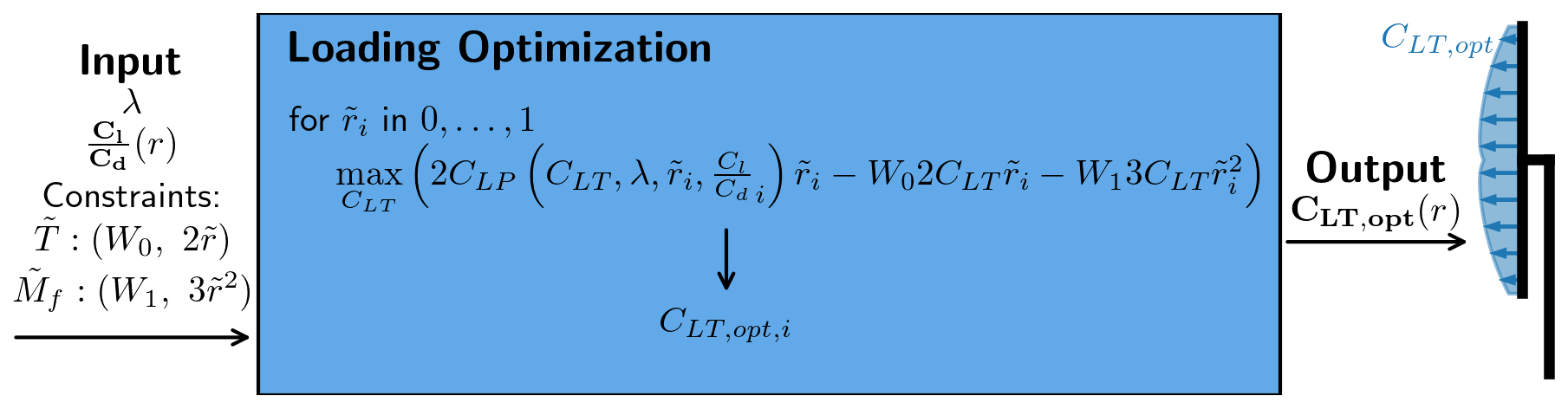
Figure 2 Flowchart for the loading optimization with a given set of inputs. Aerodynamic input: λ, $C_{\mathrm{l}}/C_{\mathrm{d}}$; constraints input: $\stackrel{\mathrm{̃}}{T}\le {\stackrel{\mathrm{̃}}{T}}_{\mathrm{0}}\to W_{\mathrm{0}}$, f_X=1, ${\stackrel{\mathrm{̃}}{M}}_f\le {\stackrel{\mathrm{̃}}{M}}_{f,\mathrm{0}}\to W_{\mathrm{1}}$, $f_X=\stackrel{\mathrm{̃}}{r}$.

Introducing the local Lagrange objective function (ℒ_L) the optimization problem at each radial station can be formulated as

$$\begin{array}{}\text{(13)}& \begin{array}{rl}\underset{{\mathit{C}}_{\mathrm{LT}}}{\max }{\mathcal{L}}_{\mathrm{L}}& =\underset{{\mathit{C}}_{\mathrm{LT}}}{\max }\left[\mathrm{2}{C}_{\mathrm{LP}}\left(C_{\mathrm{LT}}\right)\stackrel{\mathrm{̃}}{r}-\mathrm{2}{W}_{\mathrm{0}}{C}_{\mathrm{LT}}\stackrel{\mathrm{̃}}{r}\right.\\ & \left.-\mathrm{3}{W}_{\mathrm{1}}{C}_{\mathrm{LT}}{\stackrel{\mathrm{̃}}{r}}^{\mathrm{2}}\right].\end{array}\end{array}$$

To solve this problem it is assumed that C_LP is a well-behaved function, like the function presented in Part 1, which means that the problem can be solved as

$$\begin{array}{}\text{(14)}& \begin{array}{rl}\underset{{\mathit{C}}_{\mathrm{LT}}}{\max }{\mathcal{L}}_{\mathrm{L}}\Rightarrow & {\displaystyle \frac{\partial {\mathcal{L}}_{\mathrm{L}}}{\partial C_{\mathrm{LT}}}}=\mathrm{2}\stackrel{\mathrm{̃}}{r}{\displaystyle \frac{\partial C_{\mathrm{LP}}}{\partial C_{\mathrm{LT}}}}-\mathrm{2}{W}_{\mathrm{0}}\stackrel{\mathrm{̃}}{r}-\mathrm{3}{W}_{\mathrm{1}}{\stackrel{\mathrm{̃}}{r}}^{\mathrm{2}}=\mathrm{0}\\ & C_{\mathrm{LT}}\in \left[-{\displaystyle \frac{\mathrm{8}}{\mathrm{9}}},{\displaystyle \frac{\mathrm{8}}{\mathrm{9}}}\right],\end{array}\end{array}$$

where the $-\frac{\mathrm{8}}{\mathrm{9}}$ lower limit is an arbitrary lower limit. By using $\frac{\partial C_{\mathrm{LP}}}{\partial C_{\mathrm{LT}}}$ from Part 1, Eq. (26), the optimization problem can be reduced to a root-finding problem, which can be solved though the use of a root-finding algorithm like bisection or Brent's method. From now on it is assumed that the solution for the optimization problem in Eq. (14) can be solved for any level of resolution in $\stackrel{\mathrm{̃}}{r}$ for a given input of W₀, W₁. It therefore makes a function that takes W₀ and W₁ as input and returns the optimal C_LT distribution, denoted by C_LT,opt. As mentioned before, these C_LT distributions will also be a solutions to the original problem as presented in Eq. (8) for a set of constraint limits. A flowchart showing how C_LT,opt is found for a given set of inputs can be seen in Fig. 2.

2.2.5 The optimization problem with a function for optimal loading

With the C_LT,opt function mapping the input W₀ and W₁ to an optimal C_LT distribution, the optimization problem presented in Eq. (8 can be changed from an optimization for a distribution (C_LT) to an optimization in two scalars (W₀, W₁), which is a significant simplification of the original problem:

$$\begin{array}{c}\text{(15)}& {\displaystyle }\underset{W_{\mathrm{0}},W_{\mathrm{1}}}{\max }{C}_{\mathrm{P}}\left(W_{\mathrm{0}},W_{\mathrm{1}}\right)\cdot {\stackrel{\mathrm{̃}}{R}}^{\mathrm{2}}{\stackrel{\mathrm{̃}}{V}}^{\mathrm{3}},{\displaystyle }\mathrm{subj}.\begin{array}{ll}{C}_{\mathrm{T}}\left(W_{\mathrm{0}},W_{\mathrm{1}}\right)\cdot {\stackrel{\mathrm{̃}}{R}}^{\mathrm{2}}{\stackrel{\mathrm{̃}}{V}}^{\mathrm{2}}& \le {\stackrel{\mathrm{̃}}{T}}_{\mathrm{0}}\\ C_{\mathrm{FM}}\left(W_{\mathrm{0}},W_{\mathrm{1}}\right)\cdot {\stackrel{\mathrm{̃}}{R}}^{\mathrm{3}}{\stackrel{\mathrm{̃}}{V}}^{\mathrm{2}}& \le {\stackrel{\mathrm{̃}}{M}}_{\mathrm{f},\mathrm{0}}\end{array}\\ {\displaystyle }\Downarrow \\ \text{(16)}& {\displaystyle }{\stackrel{\mathrm{̃}}{P}}_{\mathrm{opt}}(\stackrel{\mathrm{̃}}{V},\stackrel{\mathrm{̃}}{R}).\end{array}$$

The optimization problem can be solved with most optimization algorithms capable of solving constraint optimization problems. All the optimization problems solved in this paper are solved with the use of the Python SciPy optimizer (Virtanen et al., 2020). A flowchart showing the optimization process can be seen in Fig. 3. Note that it is dependent on the loading optimization, meaning that this is a nested optimization loop. The output from the optimization is the optimal power (${\stackrel{\mathrm{̃}}{P}}_{\mathrm{opt}}$) that satisfies the constraints for a fixed rotor increase ($\stackrel{\mathrm{̃}}{R}$) and fixed wind speed ($\stackrel{\mathrm{̃}}{V}$).

Figure 3 Flowchart for power optimization. Note that the loading optimization is nested within the optimization loop. The optimizer needs to adjust the W₀ and W₁ for maximum power while the constraints are satisfied.

2.3 AEP optimization

The purpose of this section is to extend the optimization methodology to include optimization for maximum annual energy production (AEP) with load constraints across all wind speeds as well as fixed rated power and a fixed radius increase.

AEP is computed as the average power over a year multiplied by the time of a year. The average power can be computed from the wind distribution (f_wei, i.e., the frequency at which a wind turbine is operating at a given wind speed) and the power curve. Mathematically it can be computed as

$$\begin{array}{}\text{(17)}& \mathrm{AEP}=T_{\mathrm{year}}\underset{V_{\mathrm{CI}}}{\overset{V_{\mathrm{CO}}}{\int }}P\left(V,{\displaystyle \frac{\partial \mathit{T}}{\partial \mathit{r}}}\left(V\right),R\right)f_{\mathrm{wei}}\mathrm{d}V,\end{array}$$

where T_year is the time of a year, P is the power curve function, and V_CI and V_CO are the cut-in and cut-out wind speed respectively. The optimization problem for AEP optimization can be stated as

$$\begin{array}{}\text{(18)}& \begin{array}{rl}& \underset{{\displaystyle \frac{\partial \mathit{T}}{\partial \mathit{r}}}\left(V\right)}{\max }{T}_{\mathrm{year}}\underset{V_{\mathrm{CI}}}{\overset{V_{\mathrm{CO}}}{\int }}P\left(V,{\displaystyle \frac{\partial \mathit{T}}{\partial \mathit{r}}}\left(V\right)\right)\cdot f_{\mathrm{wei}}\mathrm{d}V\\ & \mathrm{subj}.\left.\begin{array}{ll}T\left(V,\frac{\partial \mathit{T}}{\partial \mathit{r}}\left(V\right)\right)& \le T_{\mathrm{0}}\\ M_{\mathrm{f}}\left(V,\frac{\partial \mathit{T}}{\partial \mathit{r}}\left(V\right)\right)& \le M_{\mathrm{f},\mathrm{0}}\\ P\left(V,\frac{\partial \mathit{T}}{\partial r}\left(V\right)\right)& \le P_{\mathrm{rated}}\end{array}\right\}\mathrm{for}\mathrm{all}V,\end{array}\end{array}$$

where it should be noted that the loading is allowed to change freely with changing wind speed, which is indicated by the $\frac{\partial \mathit{T}}{\partial \mathit{r}}\left(V\right)$. We apply the same normalization as in Sect. 2.2.2, where the wind speed is normalized with the rated wind speed for a rotor operating at max C_P and a unit rotor radius (R=1). The normalized optimization problem is given as

$$\begin{array}{}\text{(19)}& \begin{array}{rl}& {\max }_{{\mathit{C}}_{\mathrm{LT}}\left(\stackrel{\mathrm{̃}}{V}\right)}\underset{{\stackrel{\mathrm{̃}}{V}}_{\mathrm{CI}}}{\overset{{\stackrel{\mathrm{̃}}{V}}_{\mathrm{CO}}}{\int }}{C}_{\mathrm{P}}\left({\mathit{C}}_{\mathrm{LT}}\left(\stackrel{\mathrm{̃}}{V}\right)\right)\cdot {\stackrel{\mathrm{̃}}{R}}^{\mathrm{2}}{\stackrel{\mathrm{̃}}{V}}^{\mathrm{3}}{f}_{\mathrm{wei}}\mathrm{d}\stackrel{\mathrm{̃}}{V}\\ & \mathrm{subj}.\left.\begin{array}{ll}{C}_{\mathrm{T}}\left({\mathit{C}}_{\mathrm{LT}}\left(\stackrel{\mathrm{̃}}{V}\right)\right)\cdot {\stackrel{\mathrm{̃}}{R}}^{\mathrm{2}}{\stackrel{\mathrm{̃}}{V}}^{\mathrm{2}}& \le {\stackrel{\mathrm{̃}}{T}}_{\mathrm{0}}\\ C_{\mathrm{FM}}\left({\mathit{C}}_{\mathrm{LT}}\left(\stackrel{\mathrm{̃}}{V}\right)\right)\cdot {\stackrel{\mathrm{̃}}{R}}^{\mathrm{3}}{\stackrel{\mathrm{̃}}{V}}^{\mathrm{2}}& \le {\stackrel{\mathrm{̃}}{M}}_{\mathrm{f},\mathrm{0}}\\ C_{\mathrm{P}}\left({\mathit{C}}_{\mathrm{LT}}\left(\stackrel{\mathrm{̃}}{V}\right)\right)\cdot {\stackrel{\mathrm{̃}}{R}}^{\mathrm{2}}{\stackrel{\mathrm{̃}}{V}}^{\mathrm{3}}& \le {\stackrel{\mathrm{̃}}{P}}_{\mathrm{0}}\end{array}\right\}\mathrm{for}\mathrm{all}\stackrel{\mathrm{̃}}{V}.\end{array}\end{array}$$

Using the assumption that C_LT can change independently with wind speed the maximization can be taken within the wind speed integration. Since the constraint is for all wind speeds, the optimization problem is now a power optimization for each wind speed.

$$\begin{array}{c}\text{(20)}& {\displaystyle }\begin{array}{rl}& \underset{{\stackrel{\mathrm{̃}}{V}}_{\mathrm{CI}}}{\overset{{\stackrel{\mathrm{̃}}{V}}_{\mathrm{CO}}}{\int }}\underset{{\mathit{C}}_{\mathrm{LT}}}{max}\left[C_{\mathrm{P}}\left({\mathit{C}}_{\mathrm{LT}}\right)\cdot {\stackrel{\mathrm{̃}}{R}}^{\mathrm{2}}{\stackrel{\mathrm{̃}}{V}}^{\mathrm{3}}\right]f_{\mathrm{wei}}\mathrm{d}\stackrel{\mathrm{̃}}{V}\\ & \mathrm{subj}.\left.\begin{array}{ll}{C}_{\mathrm{T}}\left({\mathit{C}}_{\mathrm{LT}}\left(\stackrel{\mathrm{̃}}{V}\right)\right)\cdot {\stackrel{\mathrm{̃}}{R}}^{\mathrm{2}}{\stackrel{\mathrm{̃}}{V}}^{\mathrm{2}}& \le {\stackrel{\mathrm{̃}}{T}}_{\mathrm{0}}\\ C_{\mathrm{FM}}\left({\mathit{C}}_{\mathrm{LT}}\left(\stackrel{\mathrm{̃}}{V}\right)\right)\cdot {\stackrel{\mathrm{̃}}{R}}^{\mathrm{3}}{\stackrel{\mathrm{̃}}{V}}^{\mathrm{2}}& \le {\stackrel{\mathrm{̃}}{M}}_{\mathrm{f},\mathrm{0}}\\ C_{\mathrm{P}}\left({\mathit{C}}_{\mathrm{LT}}\left(\stackrel{\mathrm{̃}}{V}\right)\right)\cdot {\stackrel{\mathrm{̃}}{R}}^{\mathrm{2}}{\stackrel{\mathrm{̃}}{V}}^{\mathrm{3}}& \le {\stackrel{\mathrm{̃}}{P}}_{\mathrm{0}}\end{array}\right\}\mathrm{for}\mathrm{all}\stackrel{\mathrm{̃}}{V}\end{array},{\displaystyle }\Downarrow \left(\mathrm{power}\mathrm{optimization}\right)\\ \text{(21)}& {\displaystyle }\begin{array}{rl}& \underset{{\stackrel{\mathrm{̃}}{V}}_{\mathrm{CI}}}{\overset{{\stackrel{\mathrm{̃}}{V}}_{\mathrm{CO}}}{\int }}\underset{{\mathit{W}}_{\mathrm{0}},{\mathit{W}}_{\mathrm{1}}}{\max }\left[C_{\mathrm{P}}\left({\mathit{W}}_{\mathrm{0}},{\mathit{W}}_{\mathrm{1}}\right)\cdot {\stackrel{\mathrm{̃}}{R}}^{\mathrm{2}}{\stackrel{\mathrm{̃}}{V}}^{\mathrm{3}}\right]f_{\mathrm{wei}}\mathrm{d}\stackrel{\mathrm{̃}}{V}\\ & \mathrm{subj}.\left.\begin{array}{ll}{C}_{\mathrm{T}}\left({\mathit{W}}_{\mathrm{0}},{\mathit{W}}_{\mathrm{1}}\right)\cdot {\stackrel{\mathrm{̃}}{R}}^{\mathrm{2}}{\stackrel{\mathrm{̃}}{V}}^{\mathrm{2}}& \le {\stackrel{\mathrm{̃}}{T}}_{\mathrm{0}}\\ C_{\mathrm{FM}}\left({\mathit{W}}_{\mathrm{0}},{\mathit{W}}_{\mathrm{1}}\right)\cdot {\stackrel{\mathrm{̃}}{R}}^{\mathrm{3}}{\stackrel{\mathrm{̃}}{V}}^{\mathrm{2}}& \le {\stackrel{\mathrm{̃}}{M}}_{\mathrm{f},\mathrm{0}}\\ C_{\mathrm{P}}\left({\mathit{W}}_{\mathrm{0}},{\mathit{W}}_{\mathrm{1}}\right)\cdot {\stackrel{\mathrm{̃}}{R}}^{\mathrm{2}}{\stackrel{\mathrm{̃}}{V}}^{\mathrm{3}}& \le {\stackrel{\mathrm{̃}}{P}}_{\mathrm{0}}\end{array}\right\}\mathrm{for}\mathrm{all}\stackrel{\mathrm{̃}}{V},\end{array}\end{array}$$

where the boldface W₀ and W₁ signify that it is changing with wind speed.

It can be further simplified as

$$\begin{array}{}\text{(22)}& {\stackrel{\mathrm{̃}}{\mathrm{AEP}}}_{\mathrm{opt}}\left(\stackrel{\mathrm{̃}}{R}\right)=\underset{{\stackrel{\mathrm{̃}}{V}}_{\mathrm{CI}}}{\overset{{\stackrel{\mathrm{̃}}{V}}_{\mathrm{CO}}}{\int }}{\stackrel{\mathrm{̃}}{P}}_{\mathrm{opt}}(\stackrel{\mathrm{̃}}{V},\stackrel{\mathrm{̃}}{R})f_{\mathrm{wei}}\mathrm{d}\stackrel{\mathrm{̃}}{V},\end{array}$$

where the function for the output from the power optimization (${\stackrel{\mathrm{̃}}{P}}_{\mathrm{opt}}$) is used. It shows that the AEP optimization can be reduced to a power optimization for each wind speed in the integration. A flowchart for the AEP optimization can be seen in Fig. 4. The output from the optimization is denoted as ${\stackrel{\mathrm{̃}}{\mathrm{AEP}}}_{\mathrm{opt}}$.

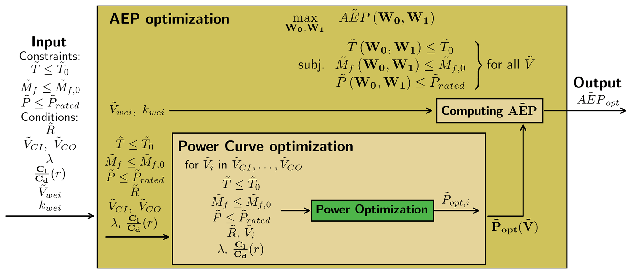
Figure 4 Flowchart for the AEP optimization. The optimization is simply a power optimization for each wind speed in the power curve.

2.4 WOwRI optimization with a simple cost function

The optimizations presented so far have been for a fixed radius increase, but in this section the optimization for rotor radius will be presented. The power optimization and AEP optimization could in principle easily be extended for radius optimization as well by simply adding the rotor radius as a design variable, but as discussed in Sect. 3.1 the optimization problem is unbounded with the global optimum at $\stackrel{\mathrm{̃}}{R}\to \mathrm{\infty }$, which is clearly not feasible for turbine design. To get a feasible rotor design, the optimization for rotor size will also include a cost function.

2.4.1 Cost function

The current work focuses on preliminary wind turbine rotor design, and a detailed cost function like the one in Fingersh et al. (2006) is therefore thought to be outside the scope of this paper. A simple cost function that is purely a function of the rotor radius is therefore proposed here.

The cost function will roughly estimate the mass increase associated with the increase in rotor radius, with the underlying assumption that mass and cost scale roughly in the same way. It is important to note here that it is not the whole turbine and associated components that need to be scaled with the change in rotor radius; as the optimization is a load-constrained optimization, the loads do not change and the associated components, therefore, do not need to be scaled.

The cost model is simply based on a cost fraction, which is the fraction of the cost that is affected by changes in radius, as well as the cost exponent, which describes how the cost (or mass) for this cost fraction scales with changes in radius. If the components affected by the radius increase are assumed to be the blades, tower and foundation, the cost fraction is found to be 39 % (using the number from Stehly and Beiter, 2020, p. 7, Fig. 1). The cost exponent is bound in the range 1–3, as an exponent of 3 would be for the case where the mass increases in all three dimensions, whereas 1 is the case where the mass is only increasing in one dimension (e.g., tip extension). With the load constraints, it is definitely less than 3, and a good estimate for the cost exponent is therefore thought to be 1.5. The suggested normalized cost function is given as

$$\begin{array}{}\text{(23)}& {\stackrel{\mathrm{̃}}{f}}_{\mathrm{cost}}\left(\stackrel{\mathrm{̃}}{R}\right)=\mathrm{0.39}\cdot {\stackrel{\mathrm{̃}}{R}}^{\mathrm{1.5}}+\mathrm{0.61}.\end{array}$$

It is important to note that this is a rough estimate for a cost function, and more importantly it has a great impact on the optimal rotor radius. But as the purpose of this paper is to present the WOwRI optimization methodology, it is thought to be outside the scope of this paper to investigate it further here.

2.4.2 Rotor size optimization with cost function

The outcome from Sect. 2.2 and 2.3 was the functions ${\stackrel{\mathrm{̃}}{P}}_{\mathrm{opt}}\left(\stackrel{\mathrm{̃}}{R}\right)$ (assuming $\stackrel{\mathrm{̃}}{V}=\mathrm{1}$) and ${\stackrel{\mathrm{̃}}{\mathrm{AEP}}}_{\mathrm{opt}}\left(\stackrel{\mathrm{̃}}{R}\right)$ respectively. These functions compute the optimal power/AEP for a given set of constraints at a fixed radius increase. Using these functions the following optimization problems for the optimal radius increase can be stated as

$$\begin{array}{}\text{(24)}& {\displaystyle }& {\displaystyle }{\max }_{\stackrel{\mathrm{̃}}{R}}{\displaystyle \frac{{\stackrel{\mathrm{̃}}{P}}_{\mathrm{opt}}\left(\stackrel{\mathrm{̃}}{R}\right)}{f_{\mathrm{cost}}\left(\stackrel{\mathrm{̃}}{R}\right)}}\left(\mathrm{power}\text{-}\mathrm{per}\text{-}\mathrm{cost}\mathrm{optimization}\right),\text{(25)}& {\displaystyle }& {\displaystyle }{\max }_{\stackrel{\mathrm{̃}}{R}}{\displaystyle \frac{{\stackrel{\mathrm{̃}}{\mathrm{AEP}}}_{\mathrm{opt}}\left(\stackrel{\mathrm{̃}}{R}\right)}{f_{\mathrm{cost}}\left(\stackrel{\mathrm{̃}}{R}\right)}}\left(\mathrm{AEP}\text{-}\mathrm{per}\text{-}\mathrm{cost}\mathrm{optimization}\right),\end{array}$$

where the impact of the constraints on the optimal design is implicitly captured in ${\stackrel{\mathrm{̃}}{P}}_{\mathrm{opt}}$ and ${\stackrel{\mathrm{̃}}{\mathrm{AEP}}}_{\mathrm{opt}}$.

3 Results and discussion

In this section, the result of applying the WOwRI optimization methodology is presented. At first, the result of pure power optimization at a single wind speed is presented and discussed, and then the result of including a cost function for the so-called power-per-cost optimization, which leads to a turbine blade planform design, is presented and discussed. The AEP optimization is then presented, and then at the end the AEP-per-cost optimization is presented, which leads to the optimal power curve. At the very end, how close it is possible to get to the optimal power curve with common wind turbine technology is tested.

The following shows how the WOwRI methodology can easily be applied for large investigations of the design space, which would otherwise be very computationally expensive with methods where simulation tools are coupled. The results presented here only consider the two constraints (thrust and flap moment) as presented earlier, but they can be extended to more constraints (like max chord, tip deflection, tower bottom bending moment) but are omitted here as the focus is on presenting the model.

3.1 Power optimization

This section shows the result of applying the optimization methodology described in Sect. 2.2 for increasing the rotor radius.

The input for the aerodynamic solver (Part 1, Loenbaek et al., 2021) is as simple as possible with no viscous loss ($C_{\mathrm{d}}/C_{\mathrm{l}}=\mathrm{0}$) and without tip loss for two different tip speed ratios (λ→∞, λ=5).

In Fig. 5 the optimization problem is solved for increasing values of $\stackrel{\mathrm{̃}}{R}$, and the power is relative to the baseline power (${\stackrel{\mathrm{̃}}{P}}_{\mathrm{0}}$), which is the power at $\stackrel{\mathrm{̃}}{R}=\mathrm{1}$.

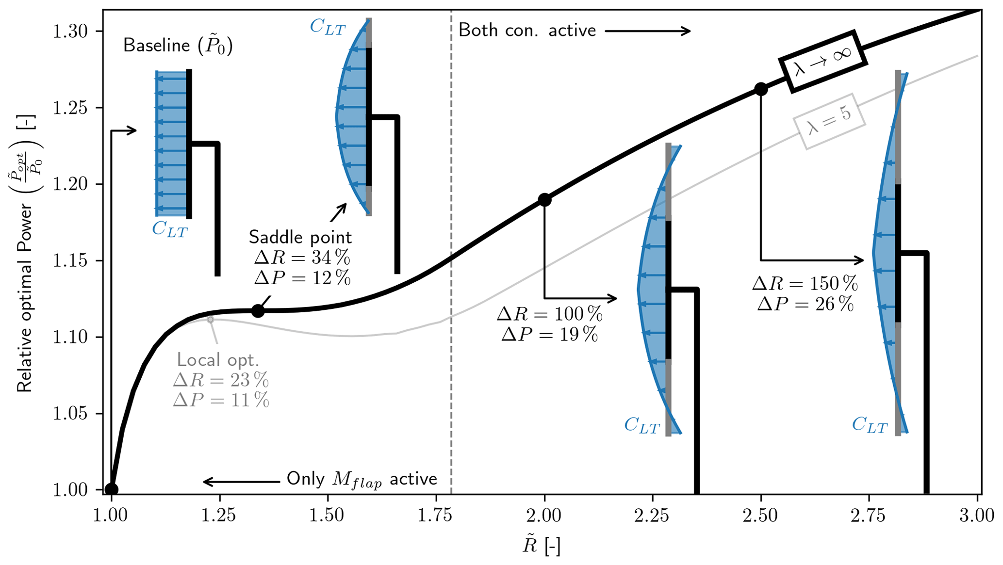
Figure 5 Optimal relative power (${\stackrel{\mathrm{̃}}{P}}_{\mathrm{opt}}/{\stackrel{\mathrm{̃}}{P}}_{\mathrm{0}}$) for increasing radius. The global optimum is at $\stackrel{\mathrm{̃}}{R}\to \mathrm{\infty }$. As expected the loading (C_LT) is seen to taper towards the tip, and for large $\stackrel{\mathrm{̃}}{R}$ the loading at the tip becomes negative.

For the case of λ→∞ (which means that there are no aerodynamic losses) it is seen that ${\stackrel{\mathrm{̃}}{P}}_{\mathrm{opt}}$ is increasing to a flat plateau (a saddle point) at $\stackrel{\mathrm{̃}}{R}=\mathrm{1.34}$ and ΔP=12 %. This is a similar result to that found by Jamieson (2020, p. 810, Sect. 3) (they parameterized axial induction and included tip loss) where the optimal solution is said to be at $\stackrel{\mathrm{̃}}{R}=\mathrm{1.34}$ and ΔP=12 %. From this analysis (without aerodynamic loss) it is found that this point is a saddle point, but including any aerodynamic loss (or non-optimal loading, like approximate optimal induction) it is found that a local optimum is formed, as can be seen for the case with λ=5 (wake rotation loss) where a local optimum is found at ΔR=23 % and ΔP=11 %.

Common to both cases is that the curve is seen to increase again beyond the saddle point/local optimum, and the curves are seen to still increase at ΔR=200 %. The global optimum is found to have an asymptotic limit as $\stackrel{\mathrm{̃}}{R}\to \mathrm{\infty }$, with the optimal power going towards the thrust constraint limit for the case without aerodynamic losses (${\stackrel{\mathrm{̃}}{P}}_{\mathrm{opt}}\to {\stackrel{\mathrm{̃}}{T}}_{\mathrm{0}}$, ΔP→50 %). Similar behavior is observed for the case with aerodynamic losses. This author observed a similar behavior using 1D momentum theory but only with a thrust constraint (Loenbaek et al., 2020, p. 163, Fig. 6), which was also observed by Jamieson (2020, p. 809). To understand why this is also the case when the loading is allowed to vary along the span with thrust and flap moment constraints, it should be noted that the loading at the tip is negative for large radius increases. The negative loading makes it possible to find a set of load distributions where the flap moment is zero (C_FM=0), but crucially it can still have a positive power (C_P>0). This is all possible while making the thrust loading arbitrary small (C_T←0), which in turn means it is always possible to satisfy the constraints for any rotor radius increase while having a positive power (${\stackrel{\mathrm{̃}}{P}}_{\mathrm{opt}}\to {\stackrel{\mathrm{̃}}{T}}_{\mathrm{0}}$). Applying a similar argument for the case without a thrust constraint, it can be found that the power will grow unbounded (${\stackrel{\mathrm{̃}}{P}}_{\mathrm{opt}}\to \mathrm{\infty }$) since the power coefficient remains finite for increasing rotor radius ($C_{\mathrm{FM}}=\mathrm{0}\to C_{\mathrm{P}}>\mathrm{0}$).

The unbounded behavior of P_opt clearly leads to unfeasible designs, and for the coming rotor design example a cost function is included to make a realistic rotor design.

3.2 Rotor design with cost function

This section will show the result of applying WOwRI for power-per-cost (PpC) optimization at a single wind speed (assumed to be $\stackrel{\mathrm{̃}}{V}=\mathrm{1}$).

For the rotor design, the aerodynamic losses will be included (i.e., wake rotation loss, viscous loss, tip loss). To include viscous loss, the glide ratio ($C_{\mathrm{l}}/C_{\mathrm{d}}$) needs to be given as input, and to get a realistic input for the glide ratio the DTU 10 MW reference turbine (Bak et al., 2013) is used as a basis, in particular the aerodynamic polars as well as the relative airfoil profile thickness distribution along the span. The glide ratio used for this design can be seen in Fig. 6d, where the polars with relative airfoil thickness th=[24 %, 30 %, 36 %, 48 %] have been used and the design point for the polar is found as described in Bak (2013, Sect. 3.5); some smoothing is then applied to ensure the design will be continued. The C_l and α in Fig. 6 are used for creating the chord and twist distributions later.

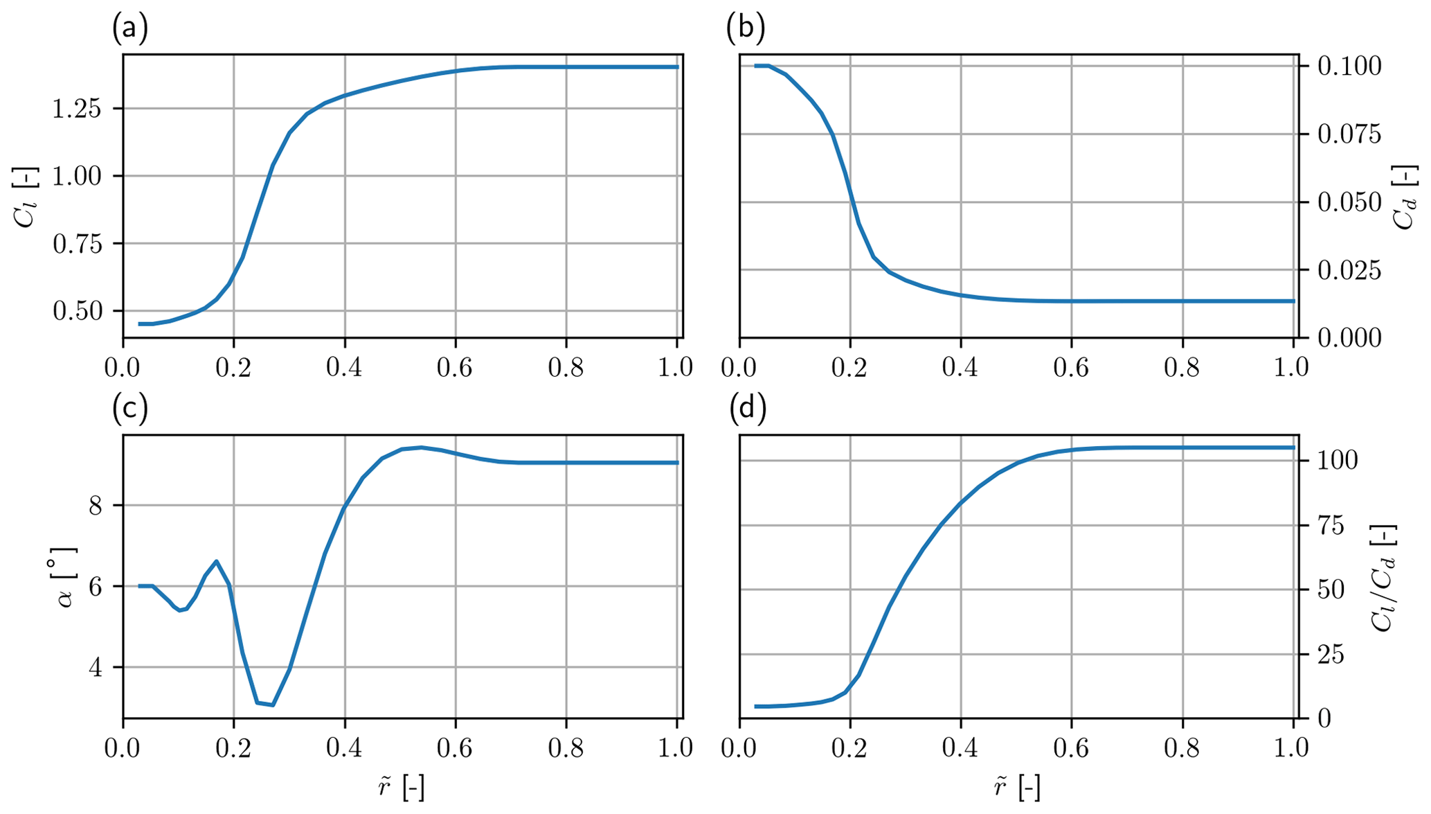
Figure 6 Aerodynamic input based on the polars from the 10 MW DTU reference turbine. (a) Lift coefficient (C_l), (b) drag coefficient (C_d), (c) angle of attack (α) and (d) glide ratio ($C_{\mathrm{l}}/C_{\mathrm{d}}$) all as a function of normalized rotor radius ($\stackrel{\mathrm{̃}}{r}$).

With the glide ratio from Fig. 6d the optimal tip speed ratio (λ) can be found as described (Part 1, Sect. 3.3). The optimal λ and the one used in this section is λ=8.23.

A plot of the relative power per cost $\left(\frac{{\stackrel{\mathrm{̃}}{P}}_{\mathrm{opt}}}{{\stackrel{\mathrm{̃}}{P}}_{\mathrm{0}}{f}_{\mathrm{cost}}}\right)$ for increasing rotor radius can be seen in Fig. 7. The optimum is found at a radius increase of ΔR=7.9 %, leading to an increase in power per cost of ΔPPC=4.2 % and a power increase of ΔP=9.0 %. From the plot it can also be seen that around $\stackrel{\mathrm{̃}}{R}\approx \mathrm{1.21}$ the impact of increasing the rotor radius leads to a lower power per cost relative to the baseline.

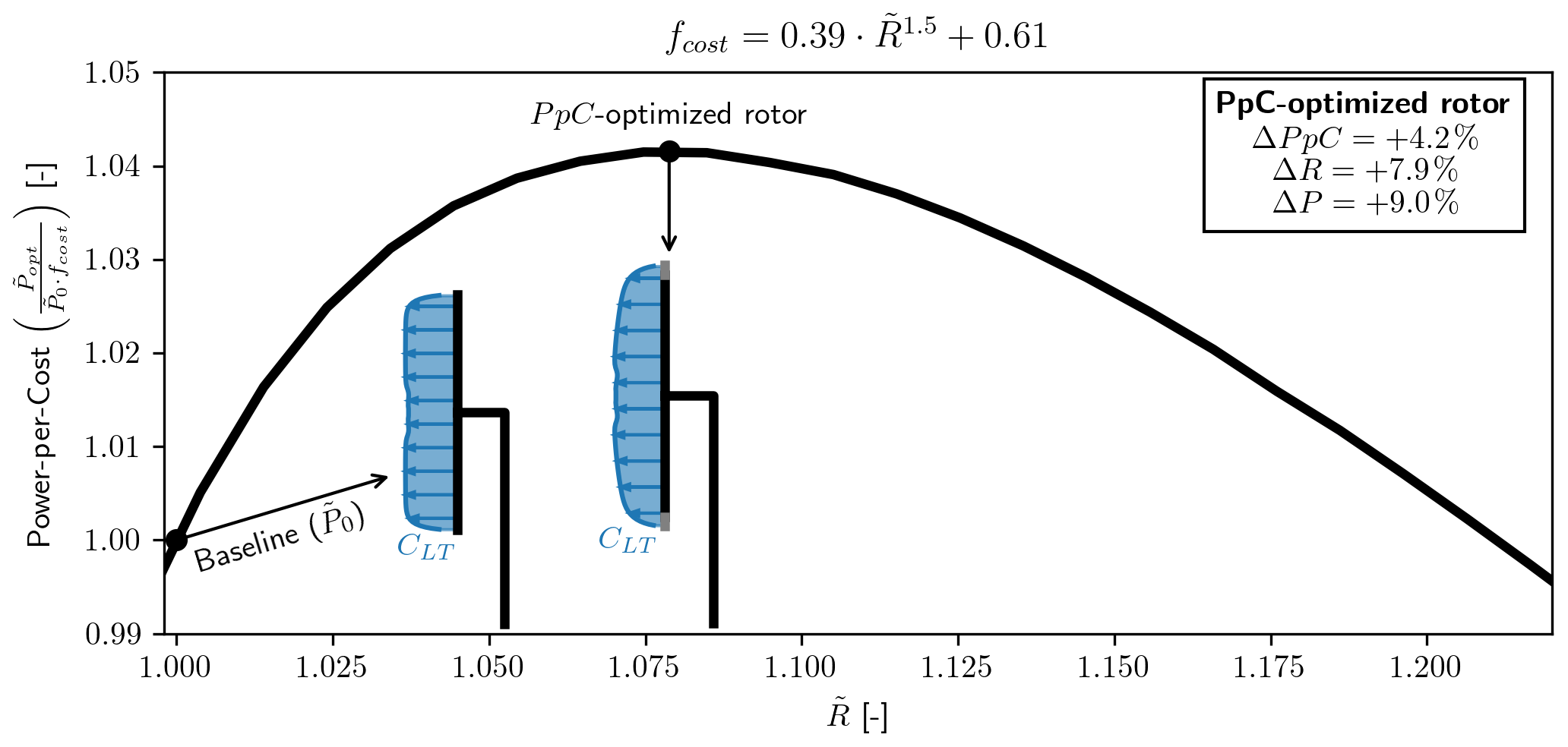
Figure 7 Relative power per cost (PpC) vs. radius ($\stackrel{\mathrm{̃}}{R}$). The cost-optimized rotor is found to have a $\mathrm{\Delta }R=+\mathrm{7.9}$ % increase in rotor radius, leading to a $\mathrm{\Delta }\mathrm{PpC}=+\mathrm{4.2}$ % increase.

A comparison of the loading distribution is shown in Fig. 8. The plot shows that the loading distribution tapers towards the tip for the optimal design relative to the baseline design. Figure 8a shows the thrust loading density ($\partial T/\partial r$) per blade (assuming three blades) and Fig. 8b the power density ($\partial P/\partial r$) per blade as a function of the rotor radius (r). The solid black line is the value for the PpC-optimized rotor, and the difference to the baseline is highlighted with shaded regions, where green indicates a positive impact and red indicates a negative impact. The striking thing to see here is how large the decrease is (the shaded green region) in Fig. 8a and how little impact this lower loading has on the loss of power in Fig. 8b (shaded red region). This has all to do with the fact that operating at maximum C_LP a change in C_LT will not lead to a proportional change in C_LP, much like the observation made by this author in (Loenbaek et al., 2020, p. 157, Fig. 1) using only 1D momentum theory. Another interesting thing is that it is only the M_f constraint that is active, which means that this PpC-optimized rotor also comes with a lower thrust of $\mathrm{\Delta }T=-\mathrm{3.8}$ %.

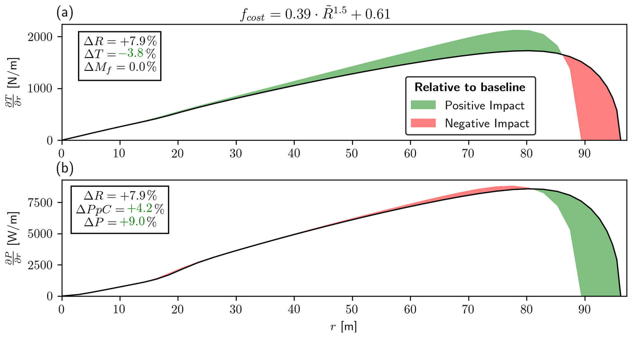
Figure 8 (a) Thrust loading density ($\partial T/\partial r$). (b) Power density ($\partial P/\partial r$) both as a function of rotor radius (r). The green shaded regions show a positive impact relative to the baseline, and red regions show a negative impact. The thing to note is the significant decrease in the loading (a) and how little impact the lower loading has on the power (b). This is due to the non-linear relationship between C_LT and C_LP.

The rotor planform (blade chord and twist) can be found from the loading distribution (C_LT, Fig. 7), the lift coefficient and angle of attack (C_l, α, Fig. 6a and c), through Eqs. (36) and (37) in Part 1 (Loenbaek et al., 2021, Sect. 4.1). A plot of the rotor planform can be seen in Fig. 9. The figure shows chord and twist for the PpC-optimized rotor, the baseline rotor ($\stackrel{\mathrm{̃}}{R}=\mathrm{1}$) and the DTU 10 MW reference turbine. A clear thing to see from these plots is that the optimization did not include a max chord constraint, with the max chord being ≈27 m, which is much larger than the DTU 10 MW reference turbine where the max chord is 6.2 m. Looking at Fig. 8, it is seen that the region from r<35 m has a similar loading as the baseline. Thus the optimization is not exploiting the maximum chord for significant gains, and one can safely correct these aberrations after. For r>35 m the chord is seen to be smaller than the DTU 10 MW reference for both the baseline and the PpC-optimized rotor, with the exception of the longer blade for the PpC-optimized rotor. Comparing the baseline and the PpC-optimized rotor, the chord is seen to be the same around r≈60 m, with the cost-optimized chord being slightly smaller from this point until the tip loss starts to become significant (which is the reason that the chord is going to zero at the tip). The smaller chord is an effect of the tapering C_LT for the PpC-optimized rotor. Thus, the lower loading distribution leads to a reduction in the chord. This may have structural implications (i.e., reduced strength and stiffness) that are not accounted for in this optimization.

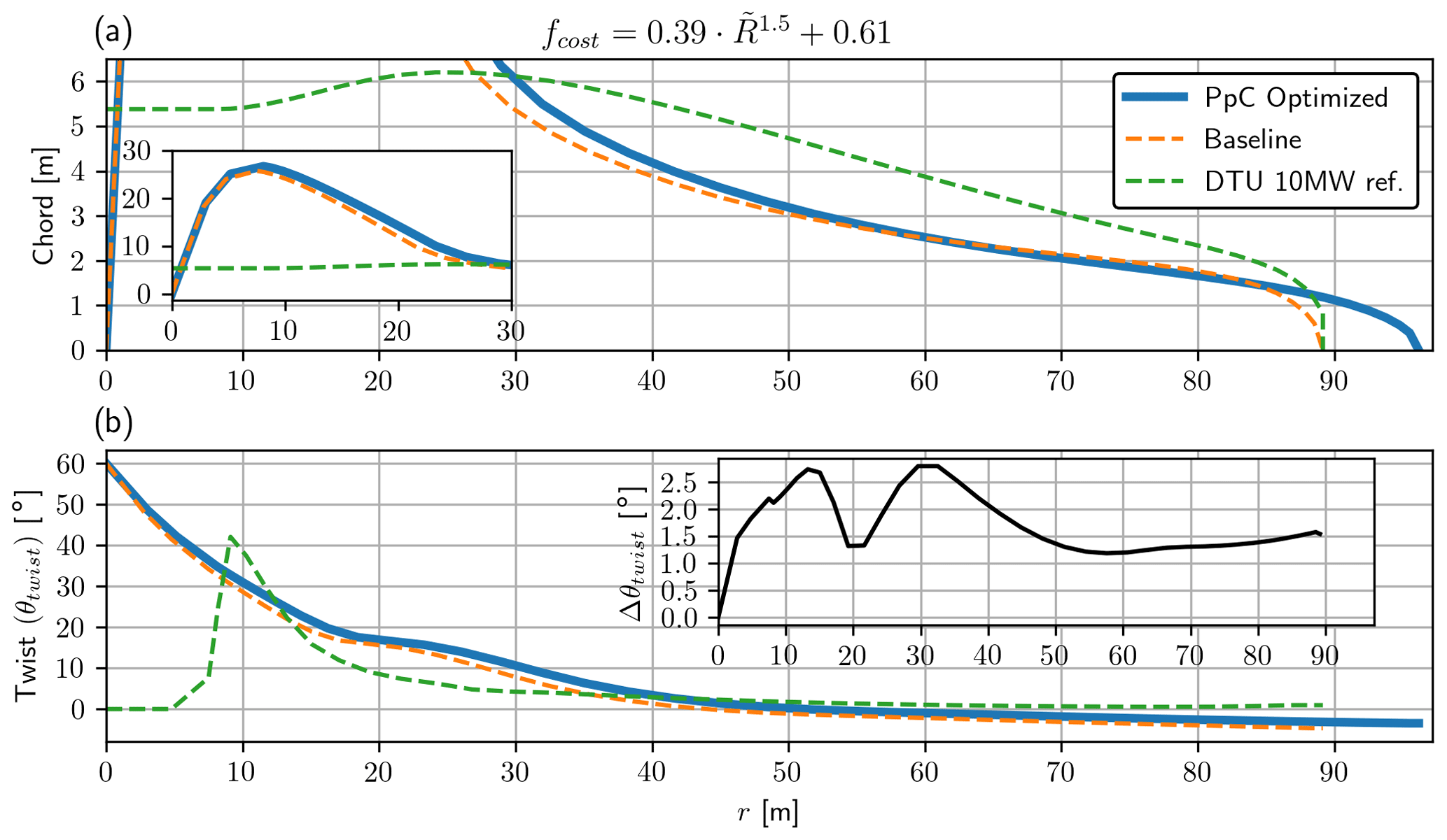
Figure 9 (a) Blade chord and (b) blade twist, both as a function of rotor radius (r) for the optimized rotor. In panel (a) an insert is added showing the chord from 0–30 m. In (b)) an insert is added which shows the difference in twist between the baseline and the PpC-optimized rotor ($\mathrm{\Delta }{\mathit{\theta }}_{\mathrm{twist}}={\mathit{\theta }}_{\mathrm{PpCopt}.}-{\mathit{\theta }}_{\mathrm{Baseline}}$).

For the twist (Fig. 9b), the difference between the baseline and PpC-optimized rotor is relatively small, with an almost constant offset of 1.5^∘ as can be seen from the Δθ_twist plot. The change is fairly small since the flow angle is approximately $\mathit{\varphi }={\tan }^{-\mathrm{1}}\mathrm{1}/\mathit{\lambda }\stackrel{\mathrm{̃}}{r}$, and the change in C_LT only has a small impact.

3.3 AEP optimization

In this section the result of solving for the optimal annual energy production (AEP) is shown, as explained in Sect. 2.3, which resulted in ${\stackrel{\mathrm{̃}}{\mathrm{AEP}}}_{\mathrm{opt}}$ (Eq. 22). The aerodynamic input is the same as for power optimization with no viscous loss ($C_{\mathrm{d}}/C_{\mathrm{l}}=\mathrm{0}$), no tip loss and no wake rotation loss (λ→∞), but also including a case with large wake rotation loss (λ=1.5) to show that a local optimum is formed when aerodynamic loss is added.

When solving the optimization problem in Eq. (22) the wind speed integration was discretized in 200 steps, which was found to make the discretization error insignificant. The integration is then performed using the trapezoidal rule.

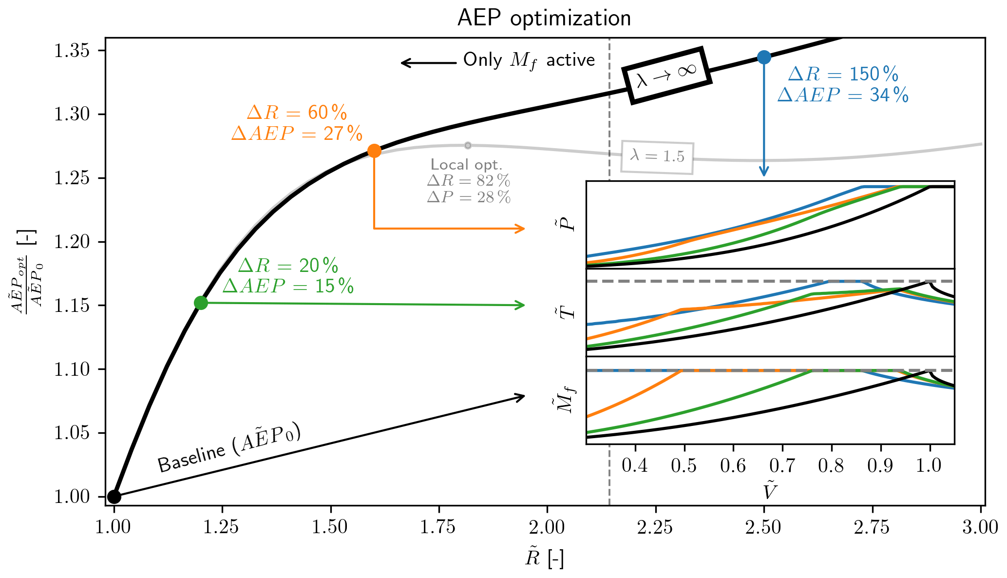
Figure 10 Optimal AEP (${\stackrel{\mathrm{̃}}{\mathrm{AEP}}}_{\mathrm{opt}}$) relative to the baseline (AEP₀, AEP at $\stackrel{\mathrm{̃}}{R}=\mathrm{1}$) vs. relative radius increase ($\stackrel{\mathrm{̃}}{R}$). The vertical dashed line shows the point where the thrust constraint starts being active; below this line it is only the flap moment constraint that is active. The power, thrust and flap moment curves are show for four selected points, which shows how these change for increasing $\stackrel{\mathrm{̃}}{R}$. An additional line shows ${\stackrel{\mathrm{̃}}{\mathrm{AEP}}}_{\mathrm{opt}}$ with λ=1.5, showing that a local optimum is formed with aerodynamic losses.

The solution for solving the AEP optimization problem can be seen in Fig. 10. The AEP optimization is seen to have similar behavior as the power optimization in Fig. 5 with an initial large slope, followed by a flatter region, and then the AEP begins to improve again. The AEP optimization does not reach a saddle point or local maximum for the case of λ→∞, as was the case for the power optimization. The slope is always positive. For the case of λ=1.5 a local optimum is found, but the formation of this local maximum required a significant amount of aerodynamic loss (λ=1.5, which leads to a large wake rotation loss) compared to the power optimization where any aerodynamic loss would lead to the formation of a local maximum.

As was the case for the power optimization the global optimum for AEP optimization is found to be a similar asymptotic limit with the optimum as $\stackrel{\mathrm{̃}}{R}\to \mathrm{\infty }$ (ΔAEP→70 %). This is the case both for λ→∞ and λ=1.5. The global optimum for the AEP optimization tends to a power curve which almost runs at rated power for all wind speeds, but the maximum power for a given wind speed is $\stackrel{\mathrm{̃}}{P}={\stackrel{\mathrm{̃}}{T}}_{\mathrm{0}}\stackrel{\mathrm{̃}}{V}$, and for a small region of the power curve the power will follow this limit before it reaches rated power. This limit is mostly of academic interest since it is not feasible for practical turbine design, and it is not investigated further here.

We turn to the power and load curves for the four highlighted points in Fig. 10. As expected, the baseline is simply operating at max C_P until rated power, creating the familiar ${\stackrel{\mathrm{̃}}{V}}^{\mathrm{3}}$ behavior for the power and ${\stackrel{\mathrm{̃}}{V}}^{\mathrm{2}}$ for the loads, where all the peak loads occur at rated conditions. However, comparing the different optimal solutions along this curve reveals different load profiles than typical modern turbines. Small increases in rotor radius increase the AEP by reaching rated power earlier. In all the extended rotor cases, the root flap-wise bending moment constraint becomes active before rated conditions are reached. Initially, this relaxes the thrust constraint. This bending moment constraint seems to limit the maximum achievable power over a greater range of the power curve. This seems to impose a minimum wind speed that rated power can be achieved; furthermore, increases in AEP must be achieved at lower wind speeds. Finally, for very large rotors, it seems that the moment constraint is active at all wind speeds, and the optimization starts to become further constrained by the thrust constraint. In general, the power curve is found to fall into three regimes in terms of wind speed ($\stackrel{\mathrm{̃}}{V}$), which are

• max C_P (no active constraints),

• maximizing power with one or more active constraints, and

• rated power.

These are the same regimes as the author found in Loenbaek et al. (2020) using a much simpler model.

3.4 Optimal power curve with cost function

In this section, the result of solving for the optimal AEP per cost (AEPpC) is presented. At first, the optimal power curve is presented, and at the end common wind turbine technology is used to see how close it can get to the optimal power curve.

The optimization will use the same aerodynamic input as in Sect. 3.2 (rotor design with cost function), with λ=8.23, glide ratio as in Fig. 6d) and including tip loss.

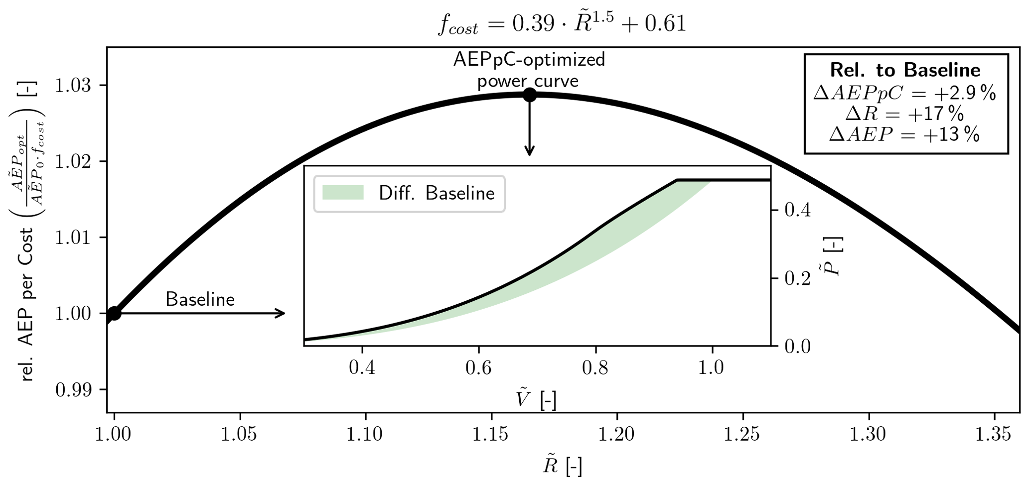
Figure 11 Relative AEP-per-cost (AEPpC) vs. relative radius increase ($\stackrel{\mathrm{̃}}{R}$). The insert shows the cost-optimized power curve with the shaded region showing the difference to the baseline power curve. The optimization is seen to reach a cost improvement of ΔAEPpC=2.9 % with a radius increase of ΔR=17 % as well as an AEP increase of ΔAEP=13 %.

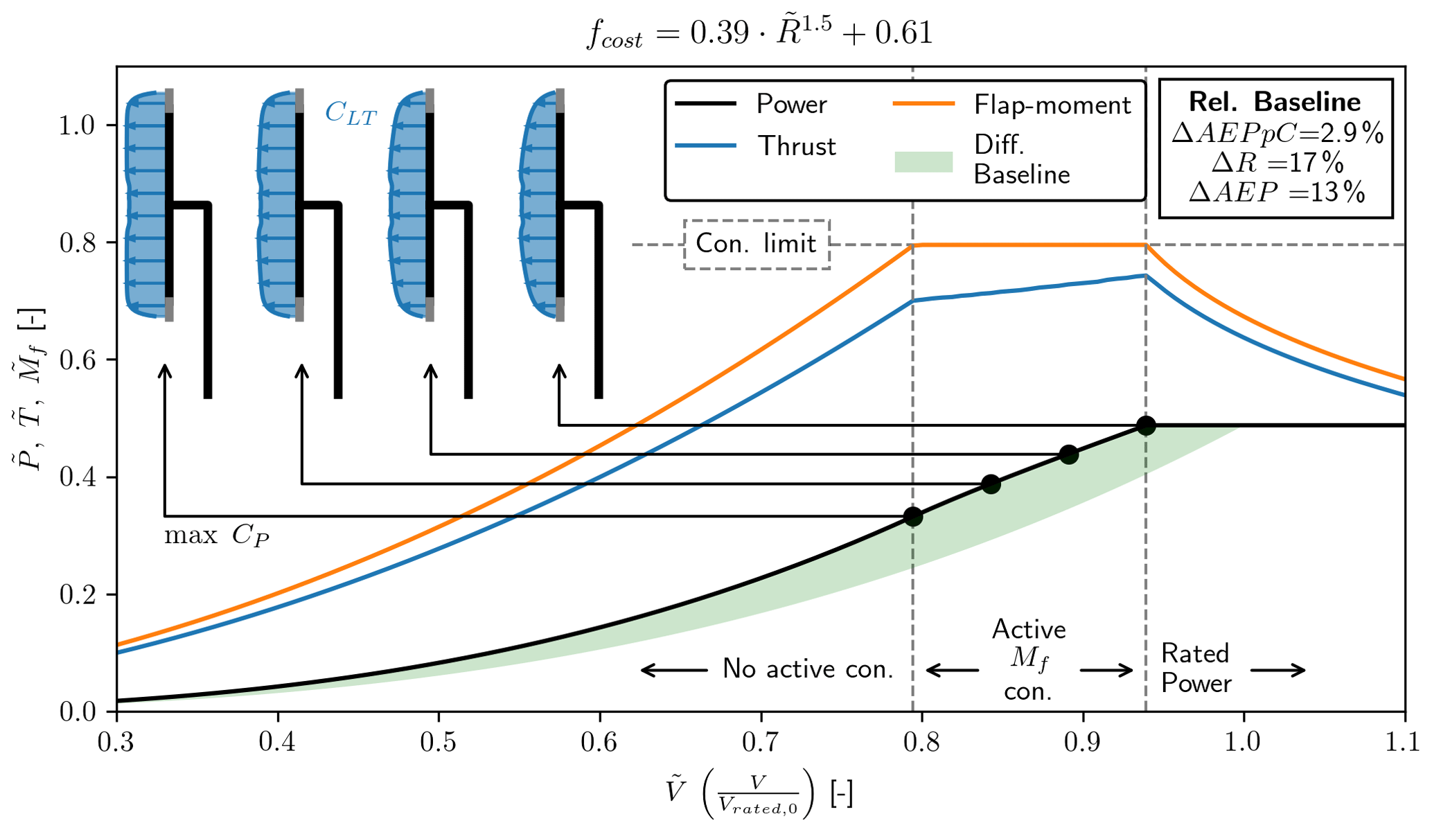
Figure 12 Normalized power ($\stackrel{\mathrm{̃}}{P}$), thrust ($\stackrel{\mathrm{̃}}{T}$) and flap moment (${\stackrel{\mathrm{̃}}{M}}_{\mathrm{flap}}$) vs. normalized wind speed ($\stackrel{\mathrm{̃}}{V}$). The transition between the three different operational regimes is indicated by the vertical dashed lines. In the region with the active constraint four points are selected, showing the optimal loading distribution (C_LT) along the rotor disc.

AEPpC for increasing values of $\stackrel{\mathrm{̃}}{R}$ can be seen in Fig. 11, where the AEPpC optimal power curve is highlighted as well as the baseline. The optimal AEPpC is found to increase by ΔAEPpC=2.9 %, with a fairly large radius increase of ΔR=17 % as well as a fairly large AEP increase of ΔAEP=13 %. In Fig. 11 it is also possible to see the power curve as well as the difference to the baseline. The increase in the power is seen to also increase for increasing $\stackrel{\mathrm{̃}}{V}$ until rated power.

Figure 12 shows this power curve along with the loads and loading distribution in greater detail. Three operational regimes can be seen in Fig. 12, separated by vertical dashed lines. The optimal power curve is seen to only have an active M_f constraint starting at $\stackrel{\mathrm{̃}}{V}\approx \mathrm{0.79}$ up until rated power at $\stackrel{\mathrm{̃}}{V}\approx \mathrm{0.94}$. In this region, the thrust curve is seen to change the slope and become linear, but it does not reach the constraint limit (vertical dashed line). The loading distribution (C_LT) for four selected points can also be seen. Starting from the point just before the M_f constraint becomes active, the loading is the one that maximizes C_P as it has been all the way up until this point. C_LT is then seen to progressively taper towards the tip as the wind speed increases.

The presented optimal power curve can not be made into a blade design as was done in Sect. 3.2, since the loading distribution was varied independently at each wind speed. The presented AEPpC optimization can therefore be seen as the idealized power curve much like the Betz limit is the idealized maximum power a turbine can achieve. It is therefore not possible, within the design constraints and aerodynamic modeling, to do any better than this optimal power curve. In the next section, it is investigated how close it is possible to get to the optimal power curve using common wind turbine technology.

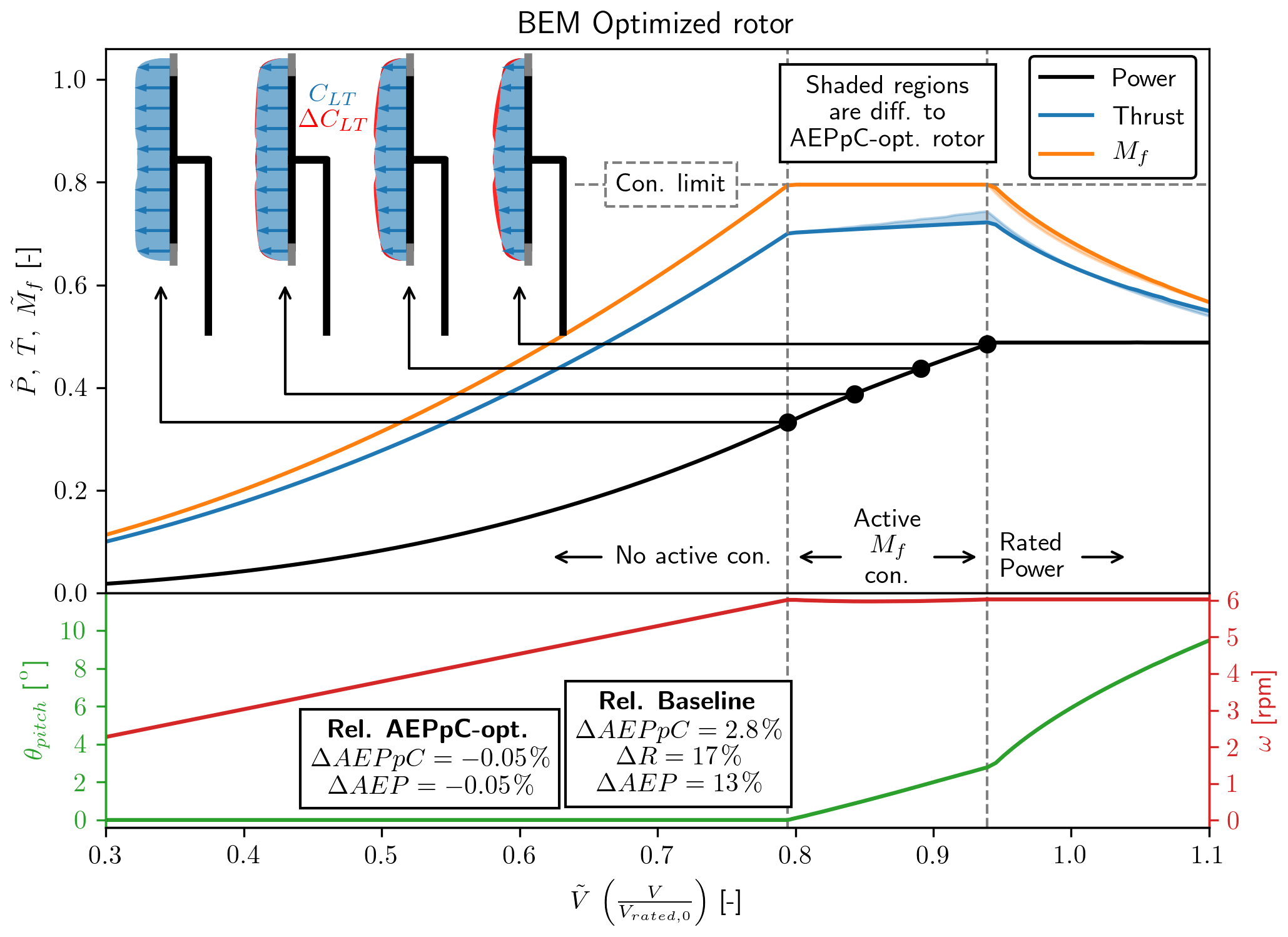
Figure 13 Power and load curves (top curves) as well as blade pitch (θ_pitch – left y axis) and rotor rotational speed (ω – right y axis) as a function normalized wind speed ($\stackrel{\mathrm{̃}}{V}$) for the BEM-optimized rotor. Rotor loading at four selected points is shown, with the red region showing the difference to the AEPpC-optimized power curve load. The difference between the AEPpC and BEM-optimized rotor in terms of AEPpC is seen to be insignificant with a difference of 0.05 %.

3.4.1 Rotor design with common wind turbine technology

For current utility scale wind turbines, there are two common parameters for altering the loading with changing wind speed, namely the blade pitch (θ_pitch) and the rotor rotational speed (ω).

To compute the aerodynamic performance for a turbine where the control parameters are the blade pitch and rotational speed, the classical blade element momentum (BEM) theory is well suited. As shown in Part 1 (Loenbaek et al., 2021, Sect. 4.2), there is a direct relationship between RIAD and BEM, and the RIAD–BEM is used for the computation of the aerodynamic performance here. BEM requires additional inputs compared to the AEPpC optimization, namely aerodynamic airfoil polars at each location along the span as well as a chord and twist along the span. The airfoil polars are taken from the DTU 10 MW reference turbine, which was the same airfoil polars used to create the glide ratio input in Fig. 6. The chord and twist are chosen to be the loading that maximizes C_P (the loading can be seen in Fig. 12 as the loading to the left). This is the same chord and twist as the baseline in Fig. 9 but with the chord linearly scaled for the radius increase.

In order to directly compare the rotor design with the optimal power curve, the radius increase is assumed to be the same as for the AEPpC optimized power curve ($\stackrel{\mathrm{̃}}{R}=\mathrm{1.17}$), and the target is then to solve a similar optimization problem as in Eq. (21) but with the design variables blade pitch and rotational speed instead. Mathematically the optimization can be stated as

$$\begin{array}{}\text{(26)}& \begin{array}{rl}& \underset{{\stackrel{\mathrm{̃}}{V}}_{\mathrm{CI}}}{\overset{{\stackrel{\mathrm{̃}}{V}}_{\mathrm{CO}}}{\int }}\underset{\mathit{\omega },{\mathit{\theta }}_{\mathrm{pitch}}}{\max }\left[C_{\mathrm{P}}\left(\mathit{\omega },{\mathit{\theta }}_{\mathrm{pitch}}\right)\cdot {\stackrel{\mathrm{̃}}{R}}^{\mathrm{2}}{\stackrel{\mathrm{̃}}{V}}^{\mathrm{3}}\right]f_{\mathrm{wei}}\mathrm{d}\stackrel{\mathrm{̃}}{V}\\ & \left.\mathrm{subj}.\begin{array}{ll}{C}_{\mathrm{T}}\left(\mathit{\omega },{\mathit{\theta }}_{\mathrm{pitch}}\right)\cdot {\stackrel{\mathrm{̃}}{R}}^{\mathrm{2}}{\stackrel{\mathrm{̃}}{V}}^{\mathrm{2}}& \le {\stackrel{\mathrm{̃}}{T}}_{\mathrm{0}}\\ C_{\mathrm{FM}}\left(\mathit{\omega },{\mathit{\theta }}_{\mathrm{pitch}}\right)\cdot {\stackrel{\mathrm{̃}}{R}}^{\mathrm{3}}{\stackrel{\mathrm{̃}}{V}}^{\mathrm{2}}& \le {\stackrel{\mathrm{̃}}{M}}_{\mathrm{f},\mathrm{0}}\\ C_{\mathrm{P}}\left(\mathit{\omega },{\mathit{\theta }}_{\mathrm{pitch}}\right)\cdot {\stackrel{\mathrm{̃}}{R}}^{\mathrm{2}}{\stackrel{\mathrm{̃}}{V}}^{\mathrm{3}}& \le {\stackrel{\mathrm{̃}}{P}}_{\mathrm{0}}\end{array}\right\}\mathrm{for}\mathrm{all}\stackrel{\mathrm{̃}}{V},\end{array}\end{array}$$

where the optimization problem is solved in the same manner shown in Fig. 4, by maximizing the power while observing the constraints at each wind speed independently.

The result of the optimization can be seen in Fig. 13, which shows the power and load curves as well as the pitch and rotational speed traces. The striking thing to note is how little the difference is between the AEPpC-optimized rotor and the BEM-optimized rotor. The difference between the two in terms of both AEP and AEPpC is seen to be 0.05%, which for all intents and purposes can be considered an insignificant difference. It means that even with this common wind turbine technology it is possible to get close to the idealized AEPpC-optimized rotor, and it, therefore, seems that the optimization methodology can almost directly be applied for rotor design. With that said, changes to the optimization problem might lead to the agreement becoming worse if the region where the constraint is active becomes larger or the limiting constraint is changed. This should be investigated further.

The optimal BEM rotor design is seen to be achieved through a θ_pitch that is almost linearly in the regime of the active M_f constraint. ω is seen to be almost constant after the M_f constraint becomes active. At four points in the regime with the active M_f constraint, the loading is shown, where the difference between the AEPpC-optimized loading and the BEM-optimized loading is shown with the shaded red area. The difference is seen to get more significant for increasing wind speeds, as one might expect. This is also the reason why if the regime of an active constraint is increased the difference between the AEPpC-optimized and BEM-optimized rotor will likely become bigger.

4 Conclusion

A novel wind turbine optimization methodology was presented. The crucial assumption that allows for this nested optimization approach is the assumption of radial independence, which is similar to the assumption made in the blade element momentum theory. It allows solving the optimal relationship between the global power (C_P) and load coefficient (C_T, C_FM) through the use of KKT multipliers, leaving an optimization problem that can be solved at each radial station independently. It allows for the original optimization problem where the optimization variables are loading distribution C_LT(r), to be changed into a KKT multipliers for each constraint (W₀, W₁, etc.).

Applying the optimization methodology for power (P) or annual energy production (AEP), without a cost function, leads to the same overall result with the global optimum being unbounded in terms of rotor radius ($\stackrel{\mathrm{̃}}{R}$) and with the global optimum being at $\stackrel{\mathrm{̃}}{R}\to \mathrm{\infty }$ with an increase in power or AEP of ΔP=50 % or ΔP=70 %, respectively.

With a simple cost function a power-per-cost (PpC) optimization resulted in a power-per-cost increase of ΔPpC=4.2 % with a radius increase of ΔR=7.9 % as well as a power increase of ΔP=9.1 %. This was obtained while keeping the same flap moment and reaching a lower thrust of $\mathrm{\Delta }T=-\mathrm{3.8}$ %. The equivalent for AEP-per-cost (AEPpC) optimization leads to increased cost efficiency of ΔAEPpC=2.9 % with a radius increase of ΔR=17 % and an AEP increase of ΔAEP=13 %, again with the same, maximum flap moment, while the maximum thrust is lower than the baseline.

Appendix A: Nomenclature

A1 Rotor global variables

Table A1 Variables that are scalars for the whole rotor. Boldface variables indicate the variable is a function or vector that changes with wind speed.

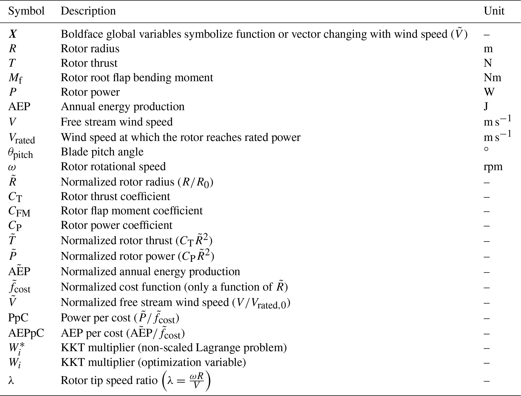
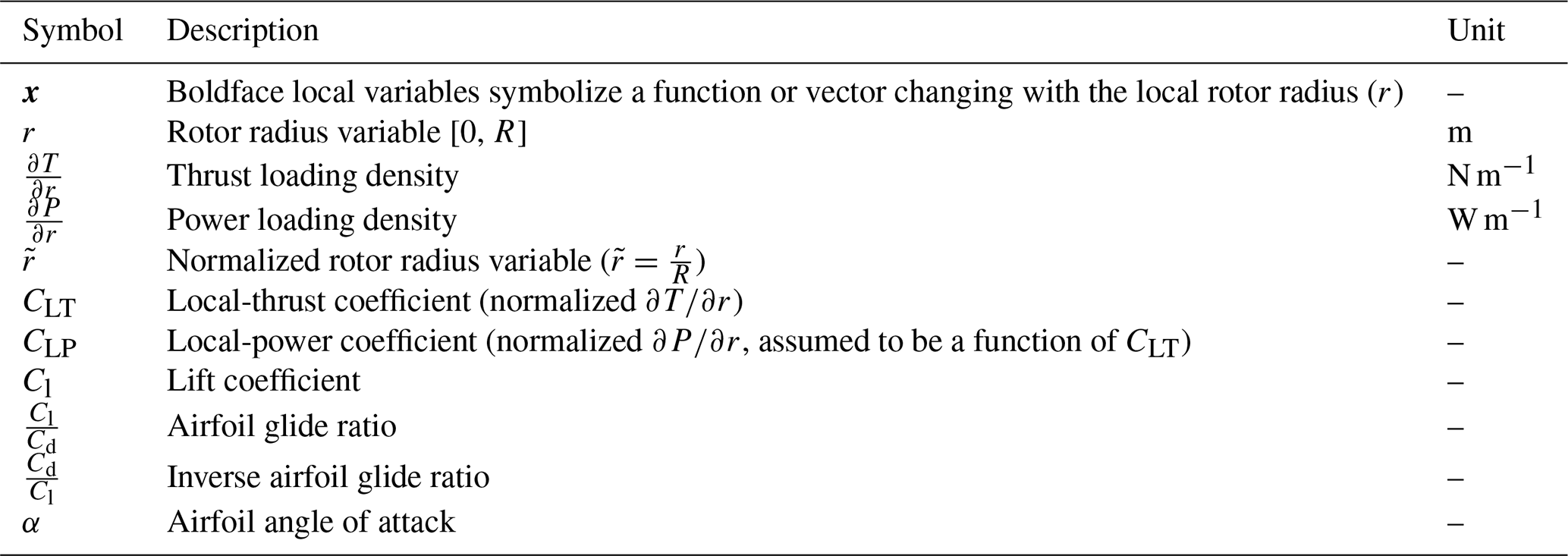
A2 Rotor local variables

Table A2 Variables that are scalars at a given radius location (r). Boldface variables indicate it is a function or vector changing with radius.