the Creative Commons Attribution 4.0 License.
the Creative Commons Attribution 4.0 License.
 | 16 Jun 2021
New methods to improve the vertical extrapolation of near-surface offshore wind speeds
Mike Optis
Nicola Bodini
Mithu Debnath
Paula Doubrawa
Accurate characterization of the offshore wind resource has been hindered by a sparsity of wind speed observations that span offshore wind turbine rotor-swept heights. Although public availability of floating lidar data is increasing, most offshore wind speed observations continue to come from buoy-based and satellite-based near-surface measurements. The aim of this study is to develop and validate novel vertical extrapolation methods that can accurately estimate wind speed time series across rotor-swept heights using these near-surface measurements. We contrast the conventional logarithmic profile against three novel approaches: a logarithmic profile with a long-term stability correction, a single-column model, and a machine-learning model. These models are developed and validated using 1 year of observations from two floating lidars deployed in US Atlantic offshore wind energy areas. We find that the machine-learning model significantly outperforms all other models across all stability regimes, seasons, and times of day. Machine-learning model performance is considerably improved by including the air–sea temperature difference, which provides some accounting for offshore atmospheric stability. Finally, we find no degradation in machine-learning model performance when tested 83 km from its training location, suggesting promising future applications in extrapolating 10 m wind speeds from spatially resolved satellite-based wind atlases.
- Article
(2112 KB) - Full-text XML
- BibTeX
- EndNote


This work was authored by the National Renewable Energy Laboratory, operated by Alliance for Sustainable Energy, LLC, for the US Department of Energy (DOE) under contract no. DE-AC36-08GO28308. The views expressed in the article do not necessarily represent the views of the DOE or the US Government. The US Government retains and the publisher, by accepting the article for publication, acknowledges that the US Government retains a nonexclusive, paid-up, irrevocable, worldwide license to publish or reproduce the published form of this work, or allow others to do so, for US Government purposes.
The accurate characterization of the offshore wind resource is crucial for a range of analyses needed to support the growing offshore wind industry. Specifically, accurate time series estimates of wind speed across the rotor-swept heights of an offshore wind turbine are used for estimates of turbine and wind plant power production, which feed into various technical and economic analyses, ranging from grid integration (Mahoney et al., 2012), life-cycle cost analyses (Jong et al., 2017), and capacity expansion studies (Hasager et al., 2015).
DNV-GL (2020)DNV-GL (2020)Atlantic Shores Offshore Wind (2020)Mayflower Offshore Wind (2020)Pacific Northwest National Laboratory (2020)Pacific Northwest National Laboratory (2020)Table 1Active floating lidar deployments in US offshore wind energy areas with publicly available data (as of December 2020).
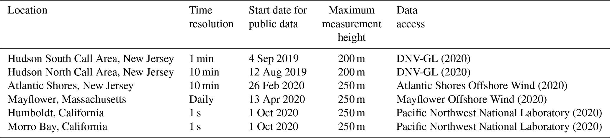
Accurate characterization of rotor-swept offshore wind speeds has been hindered by the sparsity of observations at rotor-swept heights, especially in the US offshore wind areas. Offshore meteorological towers are generally too expensive to install, especially up to 250–300 m, i.e., the expected upper rotor-swept heights of US offshore wind turbines. Buoy-mounted floating lidar, however, are emerging as a game-changing technology, especially in the United States, providing accurate wind speed and direction measurements up to approximately 250 m (Carbon Trust, 2018); however, these units are also expensive, mostly owned by wind plant developers, and their data are kept highly proprietary. In the United States, for example, as of December 2020, there are only six publicly available data sources for floating lidar in US offshore waters (Table 1).
In place of rotor-swept height measurements, near-surface observations can be used as substitutes for characterizing the offshore wind resource (Mohandes and Rehman, 2018). The main data source is the network of buoy-based wind speed measurements from the National Data Buoy Center, maintained by the National Oceanic and Atmospheric Administration (National Data Buoy Center, 1971). These data have been used to characterize the wind resource in offshore California (Wang et al., 2019; Optis et al., 2020c), the US offshore Atlantic (Optis et al., 2020b), and the Great Lakes (Doubrawa et al., 2015). These buoys generally provide years worth of wind speed measurements at heights of less than 5 m and are of high quality. In addition to these buoys, satellite-based scatterometer and synthetic-aperture radar measurements of the near-surface wind vector are increasingly being used to characterize the offshore wind resource (Doubrawa et al., 2015; Ahsbahs et al., 2017; Hasager et al., 2020; Ahsbahs et al., 2020). These data are more spatially resolved than buoy-based wind speed data, but they are limited in their temporal coverage. Further, there is some error and uncertainty in how geophysical transfer functions are used to extrapolate the satellite measurements to the diagnosed 10 m wind speed that is disseminated (Kelly and Gryning, 2010; Badger et al., 2015).
This abundance of near-surface wind speed measurements is valuable for offshore wind resource characterization provided the measurements can be accurately extrapolated to rotor-swept heights. The conventional wind industry approach – the power-law profile – is not useful in this context because the method requires measurements at two heights to calculate the shear coefficient. The logarithmic wind profile (Monin and Obukhov, 1954), by contrast, is applicable and has a long history of accurately predicting wind speeds in the atmospheric surface layer (Holtslag, 1984; Troen and Petersen, 1989; Emeis, 2013); however, the logarithmic assumption has been shown to break down at rotor-swept heights under conditions of stable stratification as turbulent fluxes decrease in magnitude and near-surface winds begin to decouple from the winds aloft (Optis et al., 2014, 2016). Under such conditions, phenomena such as low-level jets can occur, which idealized models, such as the logarithmic wind profile, are unable to account for.
Despite these shortcomings, the logarithmic profile still forms the backbone of the only novel extrapolation method that has been developed and validated for offshore applications. This novel method, developed by researchers at the Technical University of Denmark (DTU) in 2010, derives a stability-dependent long-term correction to the logarithmic wind profile (Kelly and Gryning, 2010), where stability data (e.g., Obukhov length) are provided by numerical weather prediction simulations. This model (described in more detail in Sect. 3 and herein referred to as the DTU method) has been used in subsequent studies to extrapolate 10 m diagnosed winds from satellite products with good agreement with offshore observations in Europe (Badger et al., 2015; Hasager et al., 2020). The DTU method, however, can provide only a long-term mean wind profile extrapolation and is not useful when time-series-based wind speeds across rotor-swept heights are needed (i.e., for most energy and economic offshore wind analyses).
For such applications, two novel approaches with proven success on land but not thoroughly validated offshore could be suitable. The first is a single-column model (SCM) approach, in which a typical three-dimensional numerical weather prediction model is reduced to a single vertical dimension by assuming horizontal homogeneity (Baas et al., 2010). Further assumptions (described in Sect. 3) reduce the model to a simple set of differential equations that can be run efficiently on a personal computer. The key advantage of the SCM is its ability to be forced at the lower boundary by wind and temperature observations. The SCM was used in Optis and Monahan (2016) and Optis and Monahan (2017) to extrapolate 10 m wind speeds up to 200 m at the Cabauw meteorological tower in the Netherlands. Results showed that the SCM performed about the same as the Weather Research and Forecasting (WRF) model (Skamarock et al., 2019) during a 10-year period, highlighting the benefit of local observations driving a highly simplified model.
The second novel method is based on machine learning, which has emerged as a promising approach for the vertical extrapolation of wind speeds. Bodini and Optis (2020a) and Bodini and Optis (2020b) explored this concept using four lidars and surface flux stations dispersed around the Southern Great Plains site, operated by Argonne National Laboratory. They found that a relatively simple random forest algorithm, trained on near-surface atmospheric variables, considerably outperformed the conventional power-law and logarithmic wind profiles. This performance held even when a model was trained at one measurement site and tested at others up to 100 km away, i.e., through a round-robin approach. In the offshore environment, Vassallo et al. (2020) used a deep neural network to extrapolate near-surface winds in offshore California during a 1-month period, and they also found improvement relative to conventional techniques; however, the time period was short, and a round-robin approach was not applied.
The goal of this study is to assess the viability of these conventional and more novel extrapolation models for use in US offshore areas. We provide comparisons among the different extrapolation models, and we benchmark against estimated wind profiles from the WRF model. We focus this study on the US North Atlantic and mid-Atlantic offshore areas, where the US offshore wind industry is most developed (Musial et al., 2020). In Sect. 2, we describe the domain, the observations, and the WRF model setup used. Next, in Sect. 3, we describe the various extrapolation models. Intercomparisons of model performance are provided in Sect. 4, with concluding remarks provided in Sect. 5.
2.1 Observations
To develop and validate the various extrapolation models, we leverage measurement data from two recently deployed floating lidars in offshore New Jersey and located within two current wind energy call areas (Fig. 1). These lidars were deployed by the New York State Energy Research and Development Authority (NYSERDA), which has made data publicly available in real time through a web-based access portal (DNV-GL, 2020). The portal also includes detailed technical information regarding the lidars. An overview of these floating lidars and the data available are provided in Table 2. Lidar-measured wind speeds from 20 to 200 m are used for the validation of the proposed extrapolation models (see Sect. 4), whereas the near-surface measurements at 2 m are used to develop and apply the extrapolation models (Sect. 3). Lidar-measured wind speeds are reported to have an uncertainty of 3.3 % (NYSERDA, 2021).
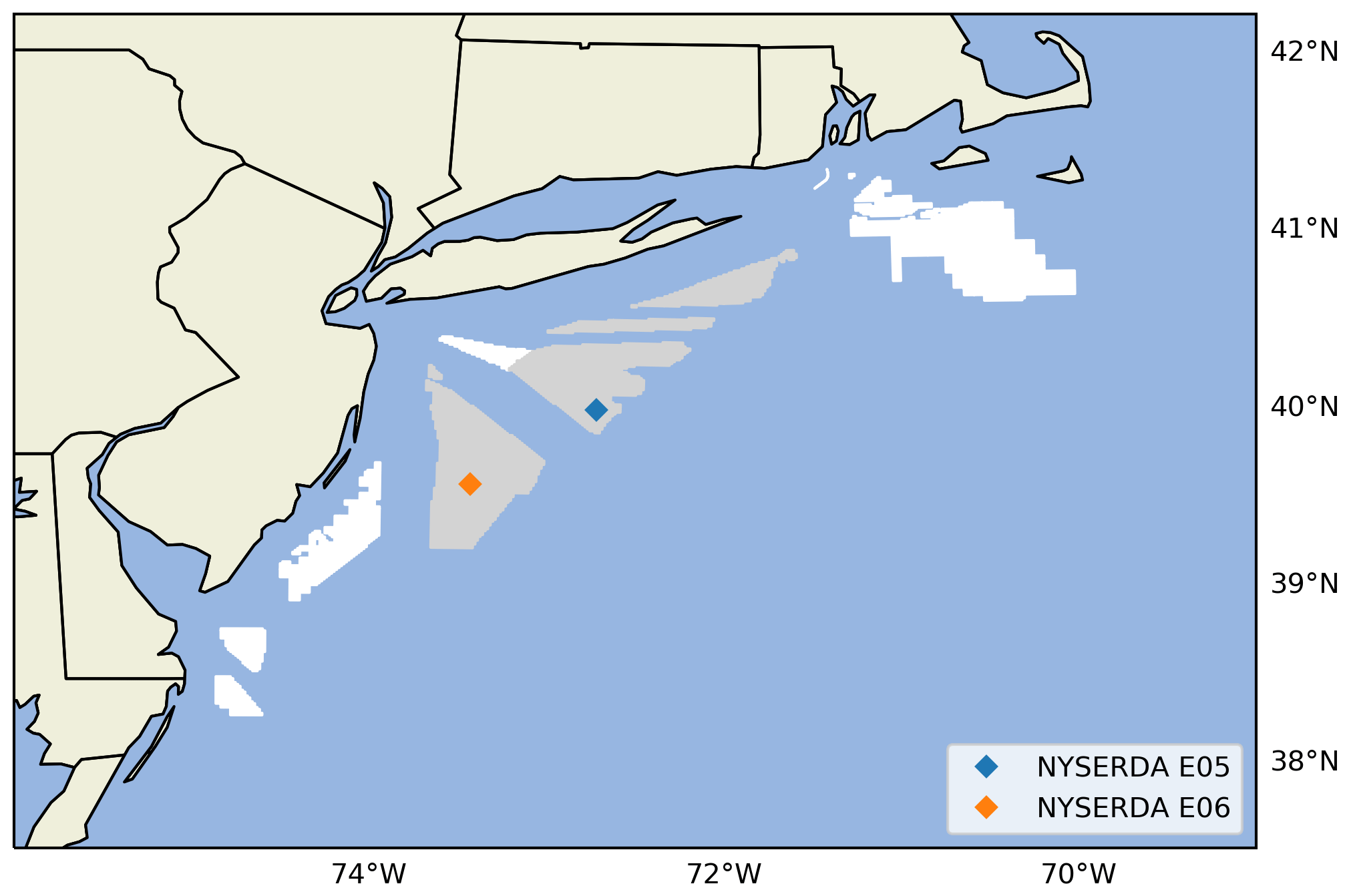
Figure 1WRF simulation domain map considered in this study. The NYSERDA lidars are shown as blue and orange diamonds. White areas denote Bureau of Ocean Energy Management wind energy lease areas; gray areas denote Bureau of Ocean Energy Management call areas.

2.2 WRF model
The WRF model is used in this study for two reasons. First, the DTU method (one of the extrapolation approaches considered in our analysis) requires surface atmospheric variables not available from the NYSERDA buoys. Second, validating the extrapolation models alongside WRF will provide key insights into the usefulness of novel extrapolation models for offshore wind energy and whether further development of these models is justified.
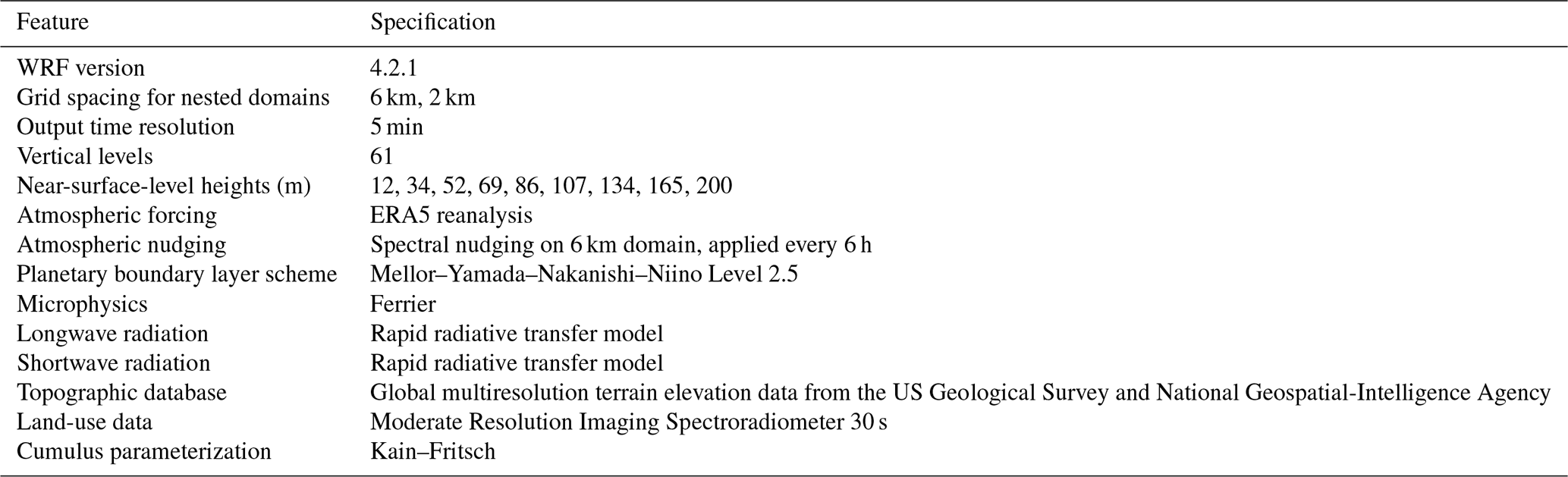
A summary of the WRF model setup is provided in Table 3, and the domain is shown in Fig. 1. The WRF model is run from 1 September 2019 through 31 August 2020, in separate monthly runs. For each month, the simulation is initialized 2 d earlier (e.g., 30 March for April simulations) and run 1 d after the end of the month (e.g., 1 May). The first day of the simulation is used to spin up the model from initial conditions, whereas the second and final days are used to stitch together the monthly runs into a single time series.
In this section we describe the different wind speed extrapolation models considered in this study. We first describe the conventional logarithmic wind profile and then discuss the DTU method, which is adopted for this study. We then discuss the most novel approaches that we have developed explicitly for this study, namely the single-column-model and machine-learning methods.
3.1 Logarithmic profile
The logarithmic wind profile is given as
where U is the wind speed, κ is the von Kármán constant (typically taken to be 0.4), z is the height above the surface, u* is the friction velocity, z0 is the roughness length, ψm is the stability function for momentum that adjusts the wind profile depending on atmospheric stability, and L is the Monin–Obukhov length that characterizes surface layer atmospheric stability. The friction velocity, u*, requires high-frequency sonic anemometer measurements that are not available at the NYSERDA buoys. To avoid specifying u*, we reformulate Eq. (1) to use the 2 m buoy wind speeds as a reference measurement, allowing the wind profile to be calculated according to
Here, we set z0=0.0001 (which is the WRF output z0 for offshore) and implement the ψm formulations from Jiménez et al. (2012), which have become standard correction functions and are currently used in the WRF mesoscale model surface layer parameterization.
The calculation of L typically requires measurements of the momentum and turbulent temperature fluxes, which are not available from buoy measurements but require high-frequency three-dimensional wind speed components and temperature measurements. Instead, we can calculate a “bulk” L based on the bulk Richardson number, RiB:
where z is the height 2 m above the surface, g is the acceleration as a result of gravity, is the potential temperature at 2 m, θsurf is the potential temperature at the surface, and U2 m is the 2 m wind speed. Combining Eqs. (2) and (3) yields the following relationship between L and RiB:
where ψh is the stability function for temperature, also taken from Jiménez et al. (2012).
Using Eq. (4), we iteratively solve for L given RiB, which combined with Eq. (2) allows for the calculation of the vertical wind profile.
3.2 DTU model
Noting the breakdown of the logarithmic wind profile in very stable conditions, the DTU method aims to preserve its applicability by applying it only in the context of a mean long-term wind profile, which is generally well estimated as logarithmic. The overall approach is to account for the distribution of L value output from WRF throughout the year. As such, the DTU method is suitable only for long-term wind resource assessment because it requires at least 1 year of data and ideally many years (Kelly and Gryning, 2010).
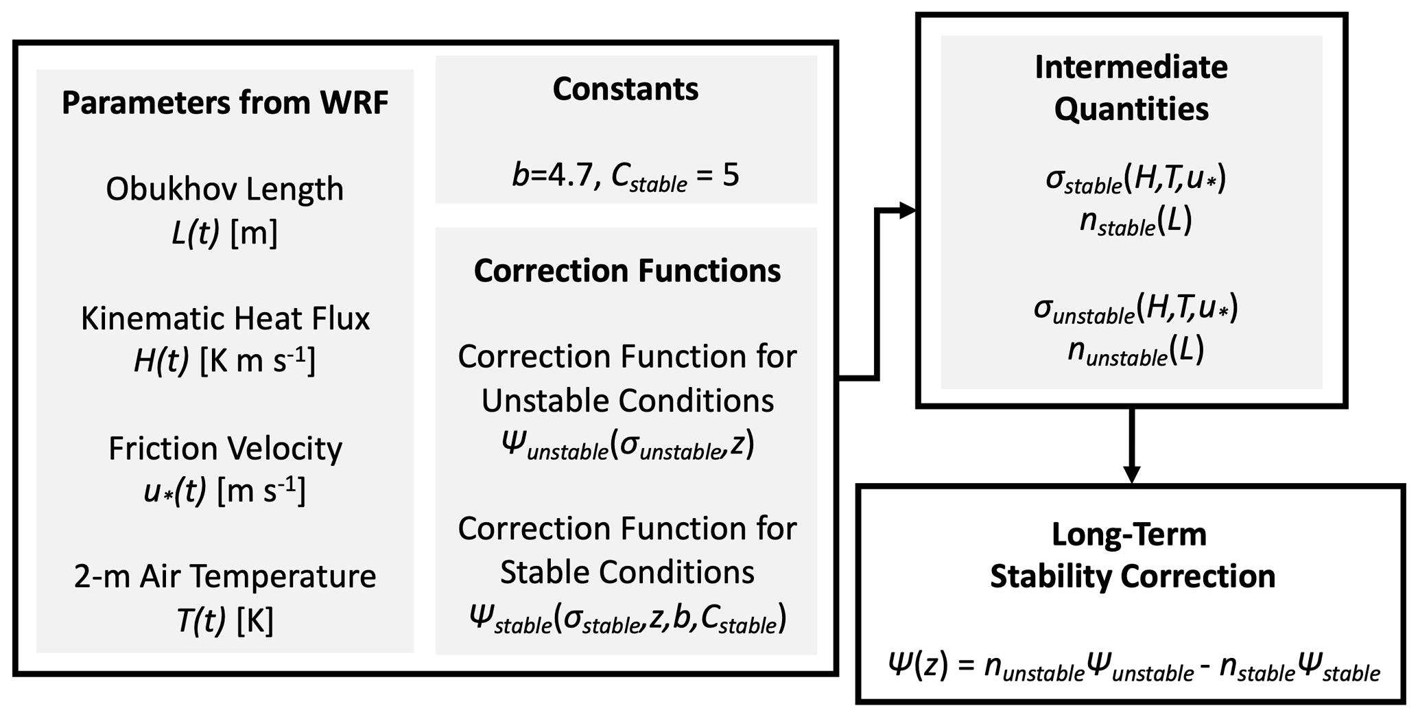
Figure 2Schematic of quantities and calculations involved in the DTU model considered herein.
The stability correction applied to the log extrapolation is height-dependent and computed based on empirical constants and atmospheric conditions at the site: the percentage of stable vs. unstable conditions; the quadratic mean of the kinematic heat flux; the mean, near-surface air temperature; and the time-averaged friction velocity. These input parameters are taken from the WRF simulations and are combined with stability functions, ψm, based on similarity theory to compute a vertical profile of the correction function (Fig. 2). This correction is then added to the log extrapolation to yield a wind speed profile, as in Eq. (1), where u* is taken from the WRF simulation, and z0 is computed using the Charnock relationship, , with g being the acceleration caused by gravity, and α=0.0144 (Charnock, 1955).
Before implementing this model, we verify that the probability distribution functions for atmospheric stability are a good fit to the empirical distributions. This comparison is given in Fig. 3. The functions shown in this figure take into account the percentage of stable vs. unstable conditions at the NYSERDA buoy sites (nstable and nunstable), scales of variation for L−1 (σstable and σunstable), and empirical constants (Cstable=5 and Cunstable=12). Note that previous work focusing on other data sets used different values for the C± constants (e.g., both were set to 3.0 in Badger et al., 2015, to extrapolate satellite-derived wind speed measurements).
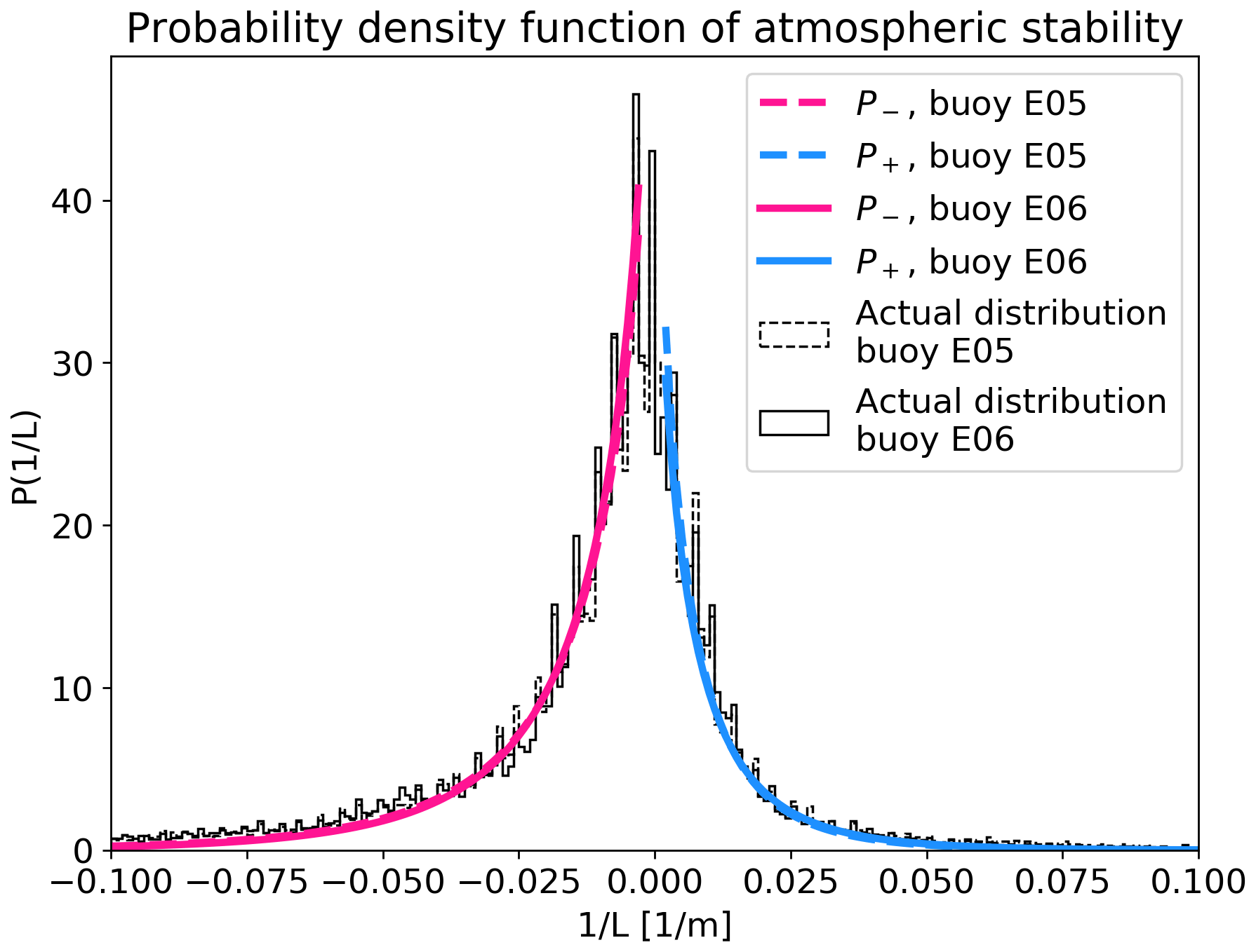
Figure 3Empirical vs. theoretical distribution of atmospheric stability for the two buoy sites.
3.3 Random forest machine-learning model
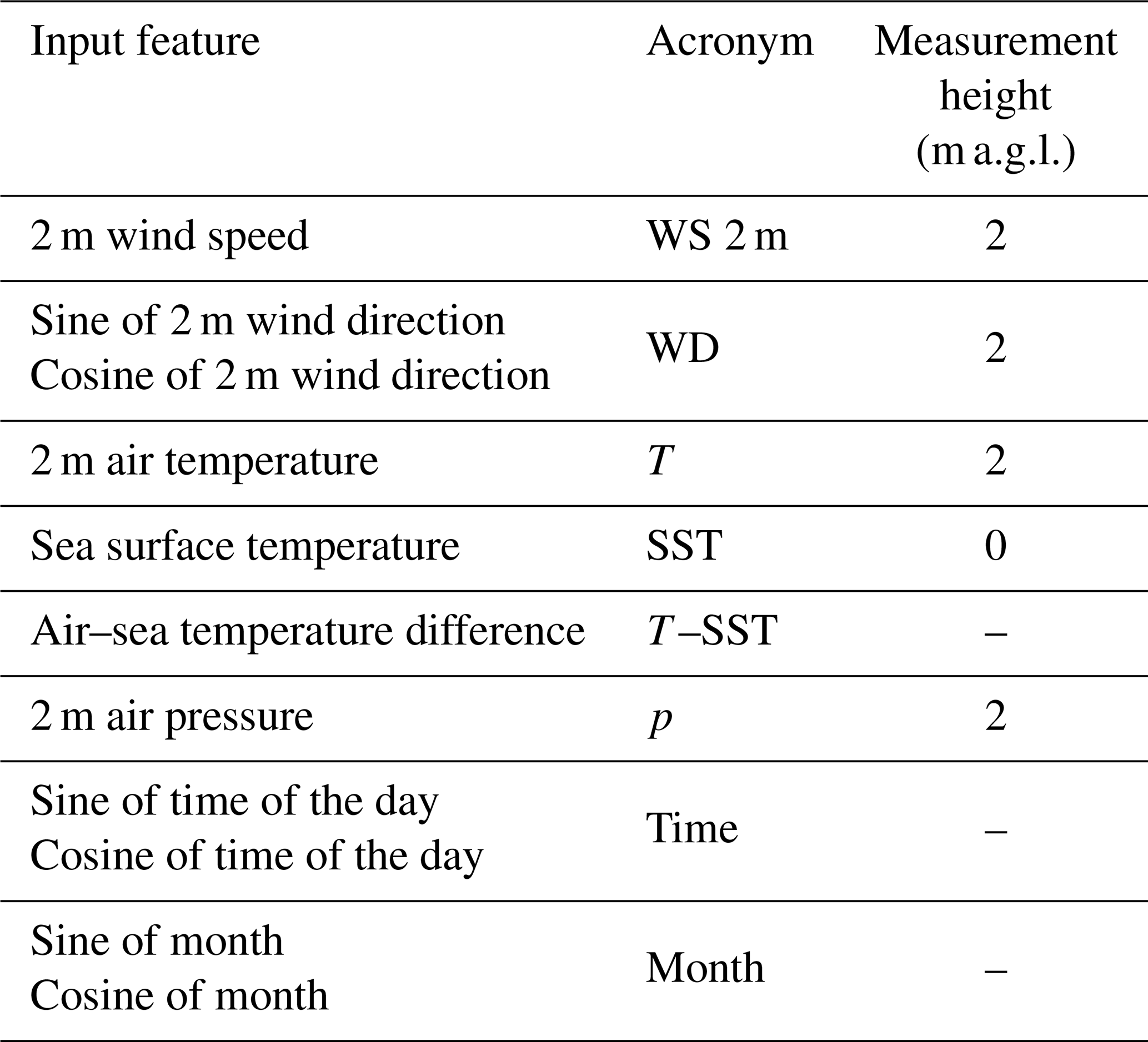
The third model considered is based on machine learning. Here, we consider a relatively simple ensemble-based regression tree method, known as a random forest model, which has shown strong predictive power in previous land-based wind speed extrapolation work (Bodini and Optis, 2020a, b) and in relating wind plant energy production to on-site atmospheric variables (Optis and Perr-Sauer, 2019). We use the RandomForestRegressor module in Python's Scikit-learn (Pedregosa et al., 2011). We consider a range of 10 min averaged input variables available from the NYSERDA buoys: 2 m wind speed, wind direction, pressure, and air temperature; the sea surface temperature and air–sea temperature difference; and the time of day and month of year. Wind direction, time of day, and month of year are all decomposed into their sine and cosine components to preserve circularity (i.e., 0 and 360∘ directions are equivalent, as are 00:00 and 24:00 LT)1. A summary of these variables is listed in Table 4.
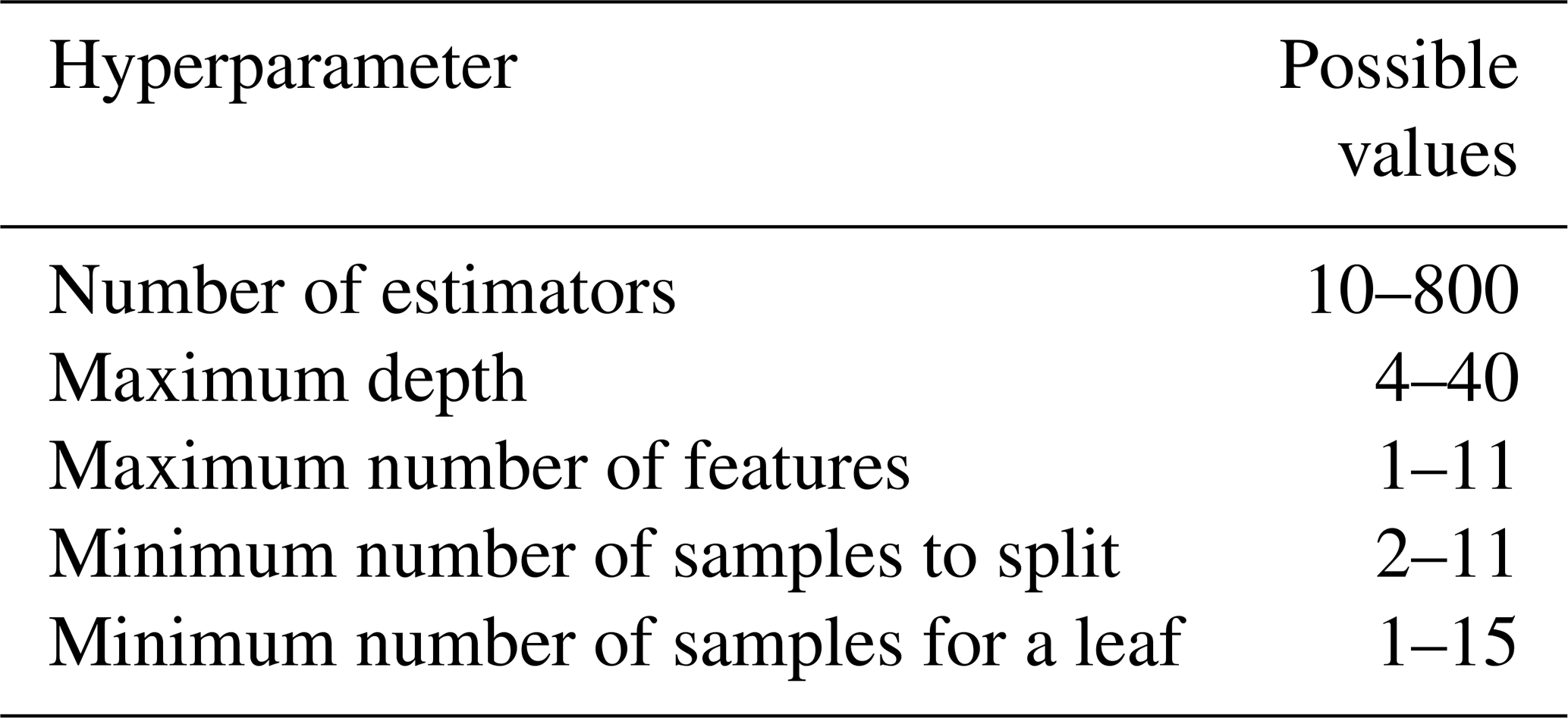
To ensure that the observation sets over which the random forest is trained and tested cover as much of the seasonal variability as possible, we build the testing set using a consecutive 20 % of the observations from each month in the period of record. We evaluate 20 randomly selected combinations of the hyperparameters with a fivefold cross-validation. The hyperparameters considered in the cross-validation and their sampled ranges are shown in Table 5. We evaluate the performance of the learning algorithm based on the root-mean-square error (RMSE) between the measured and predicted wind speed at extrapolation height: the set of hyperparameters that leads to the lowest RMSE is selected and used to assess the final performance of the learning algorithm.
Table 5Algorithm hyperparameters sampled in the random forest cross-validation.
As described in detail in Bodini and Optis (2020b), it is both impractical and unfair to evaluate a machine-learning model at the same site where it is trained. Critically, the model requires observations of the lidar-measured wind speeds up to 200 m to be trained. Evaluating model performance at the training site is impractical because the wind profiles are already known and unfair because the other extrapolation methods do not have such knowledge of lidar-measured wind profiles. Instead, model performance must be assessed through a round-robin approach, in which the model is evaluated at a site not used to train the model. Specifically, in this study, the random forest model is trained on data at NYSERDA buoy E05 and then evaluated against other extrapolation models at NYSERDA buoy E06, located 83 km away, and then vice versa. This round-robin approach ensures a fair comparison of the different extrapolation methods and that no model has prior knowledge of lidar-measured wind profiles at the site where it is evaluated.
3.4 Single-column model
The fourth model considered is an SCM. Essentially, it is a stripped-down version of a three-dimensional model, such as WRF, in which only vertical exchanges are considered and horizontal homogeneity is assumed. This greatly simplifies the governing equations of a three-dimensional model and reduces the SCM to a one-dimensional model in the vertical direction. By assuming no moisture or cloud radiation, the equations of motion simplify further and depend only on the horizontal pressure gradients, the Coriolis force, and the vertical turbulent flux of momentum and temperature:
where u, v, and w are the three vector wind components; t is time; z is the height above the surface; θ is potential temperature; and uG and vG are the u and v components of the geostrophic wind. The , terms represent the u and v components of the vertical turbulent momentum flux, and represents the vertical turbulent temperature flux.
The momentum and temperature fluxes are not solved directly but rather parameterized based on well-established eddy–diffusivity relationships:
where Km and Kh are the eddy diffusivities for momentum and temperature, respectively. These terms are themselves parameterized with a range of possible options in the literature (Optis and Monahan, 2016, 2017). We adopt a relatively simple first-order closure model that includes eddy diffusivities that are related to the wind speed gradient and a stability function that depends on the Richardson number:
where lm and lh are the mixing lengths for momentum and temperature, respectively, and fm and fh are the stability functions for momentum and temperature, respectively. There are a range of proposed formulations for the mixing lengths and stability functions. Here, we use the one developed by Smith (1990), which showed strong results when used in an SCM in previous studies (Optis and Monahan, 2016, 2017). A detailed explanation and the equations of the stability functions and mixing lengths can be found in Smith (1990), Cuxart et al. (2006), and Optis and Monahan (2017).
The SCM equations are solved on a logarithmically stretched grid from a height of 2–2000 m with 200 grid levels that provide higher resolution near the surface. The lower boundary conditions at 2 m are the measured wind speed components and temperature from the NYSERDA buoys. The upper boundary conditions are the 800 hPa pressure-level data provided by the ERA5 reanalysis. A zero-temperature gradient boundary condition is also applied at the top of the domain.
Recognizing that the geostrophic wind can change with height in conditions of horizontal temperature gradients, we calculate a geostrophic wind profile at each time step to force the simulations. This is done by first assuming that the 800 hPa winds from ERA5 are geostrophic, which is a reasonable assumption at 2000 m, where surface friction effects should be negligible. Next, we calculate the geostrophic wind at the surface using surface pressure and air temperature data from the ERA5 reanalysis product:
where ρ is air density, and P is pressure. The horizontal pressure gradient terms are calculated by taking a planar best fit of the closest nine ERA5 grid points that surround the buoy locations. Equation (8) is used to calculate the geostrophic wind components at 2 m, and finally the geostrophic wind profile is found by linearly interpolating the 2 m and 800 hPa values to the different SCM heights.
To initialize the simulation, we start by solving for the neutral vertical wind profile by imposing an equilibrium condition (i.e., ; ; ). The simulation then moves forward from the neutral profile as a time-marching algorithm using the complete set of equations provided in this section. A continuous simulation is launched for the whole year of measurements without interruption.
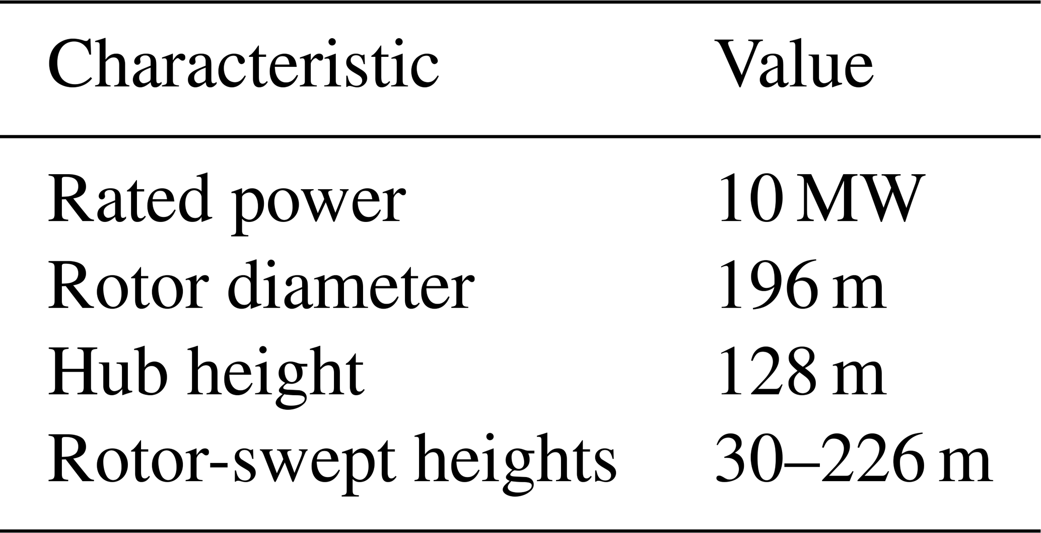
The four vertical extrapolation models presented in the previous section are all validated against lidar data from NYSERDA buoys E05 and E06 during the full period of record. For each lidar, we consider only the time periods where wind speeds are reported at every height from 20–200 m. Based on recent best-practice recommendations for validating offshore wind models (Optis et al., 2020a), we validate the rotor-equivalent wind speed (REWS) rather than an assumed hub-height wind speed. Details for calculating REWS are provided in Wagner et al. (2014). To calculate REWS, we assume a 10 MW offshore reference turbine as described in Beiter et al. (2020) and summarized in Table 6.
Table 6The 10 MW offshore reference wind turbine specifications from Beiter et al. (2020) used to calculate REWS.
We also assess model performance using the four recommended performance metrics from Optis et al. (2020a), summarized in Table 7. We note that the DTU method is capable of modeling only the mean wind profile; therefore, time-series-based performance analysis throughout this section excludes the DTU method.
Table 7Performance metrics used to assess extrapolation model performance.
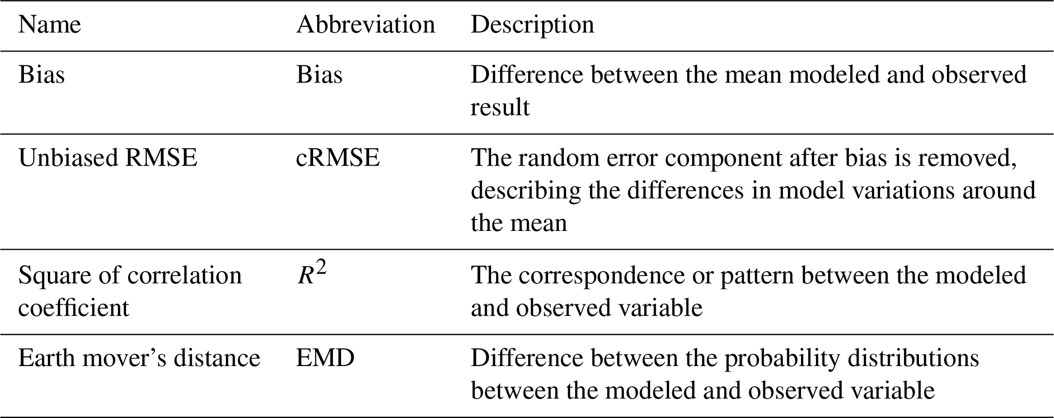
We begin with a comparison of the mean wind profile in Fig. 4, showing results at both NYSERDA buoys E05 and E06. The observed wind profile shows moderate shear, increasing from approximately 8.5 to 10.5 m s−1 at E05 and 8.0 to 10.3 m s−1 at E06. As shown, the random forest machine-learning model provides excellent agreement with the mean profile, whereas the other models are deficient in some respects. The SCM underestimates wind speeds at E05 but is very close to the observed profile at E06. The logarithmic profile captures the upper winds relatively well with a slight positive bias, but it has increasingly higher bias at lower heights. The DTU method significantly overestimates wind speeds, especially at the upper heights, with nearly a 1.5 m s−1 bias at 200 m. Finally, we see that the WRF model tends to underestimate the wind profile.
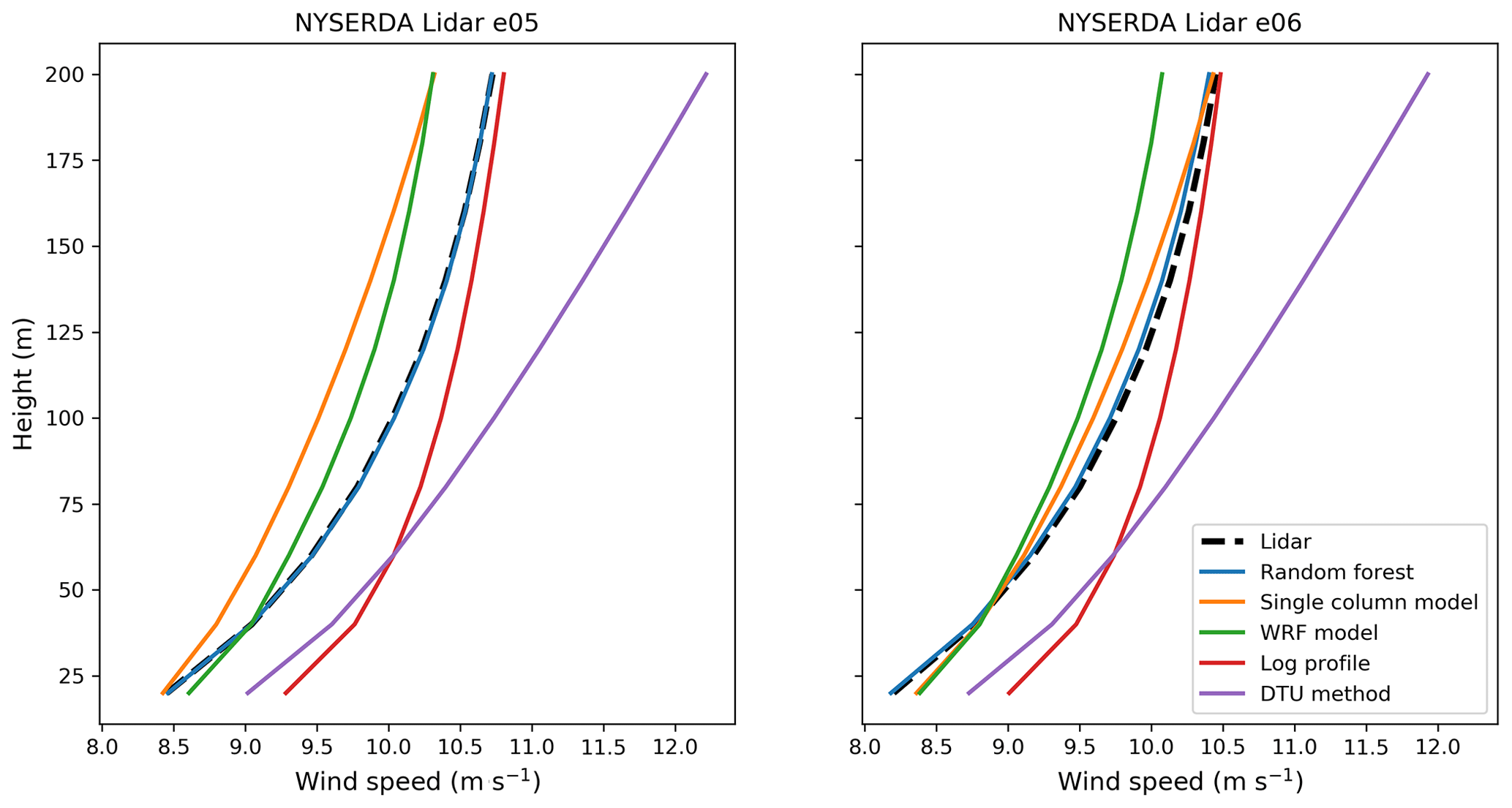
Figure 4Mean modeled and observed wind profiles at NYSERDA buoys E05 and E06. The dotted line denotes the observed profile, and solid colors denote the different extrapolation models.
REWS-based performance metrics for the different models are shown in Fig. 5. Again, the strong performance of the machine-learning model is apparent, with considerably lower error metrics and higher correlation to observations relative to the other models. The bias is notably negligible at buoy E05 and slightly negative at E06. In contrast, the SCM has the weakest performance across all metrics at E05 and all but the bias at E06. The logarithmic profile performance falls in between the machine-learning model and the SCM and is the only model with a positive bias at both buoys. Finally, the WRF model tends to perform similarly to the logarithmic model, with slightly lower unbiased RMSE and higher correlation but higher magnitude of bias and earth mover's distance (EMD).

Next, we consider the role of atmospheric stability in relative model performance. Here, we distinguish between unstable and stable conditions using the WRF-modeled bulk Richardson number, RiB, between 200 m and the surface (RiB<0 for unstable conditions; RiB>0 for stable conditions). Mean wind profiles by stability regime are shown in Fig. 6. Here, we focus only on buoy E05 and note that relative performance is similar at both buoys. The machine-learning model shows similar performance in unstable and stable conditions, accurately capturing the unstable profile and slightly underestimating the stable profile. The SCM performs reasonably well in unstable conditions but is unable to capture the high shear in the stable regime and significantly underestimates wind speeds. The log profile similarly underestimates wind speeds in stable conditions but overestimates in unstable conditions. Finally, the WRF model underestimates the wind profile in unstable conditions while accurately capturing winds greater than 100 m in stable conditions but overestimating them when less than 100 m. Overall, we see that all models apart from the random forest struggle with consistent accuracy across stability regimes.
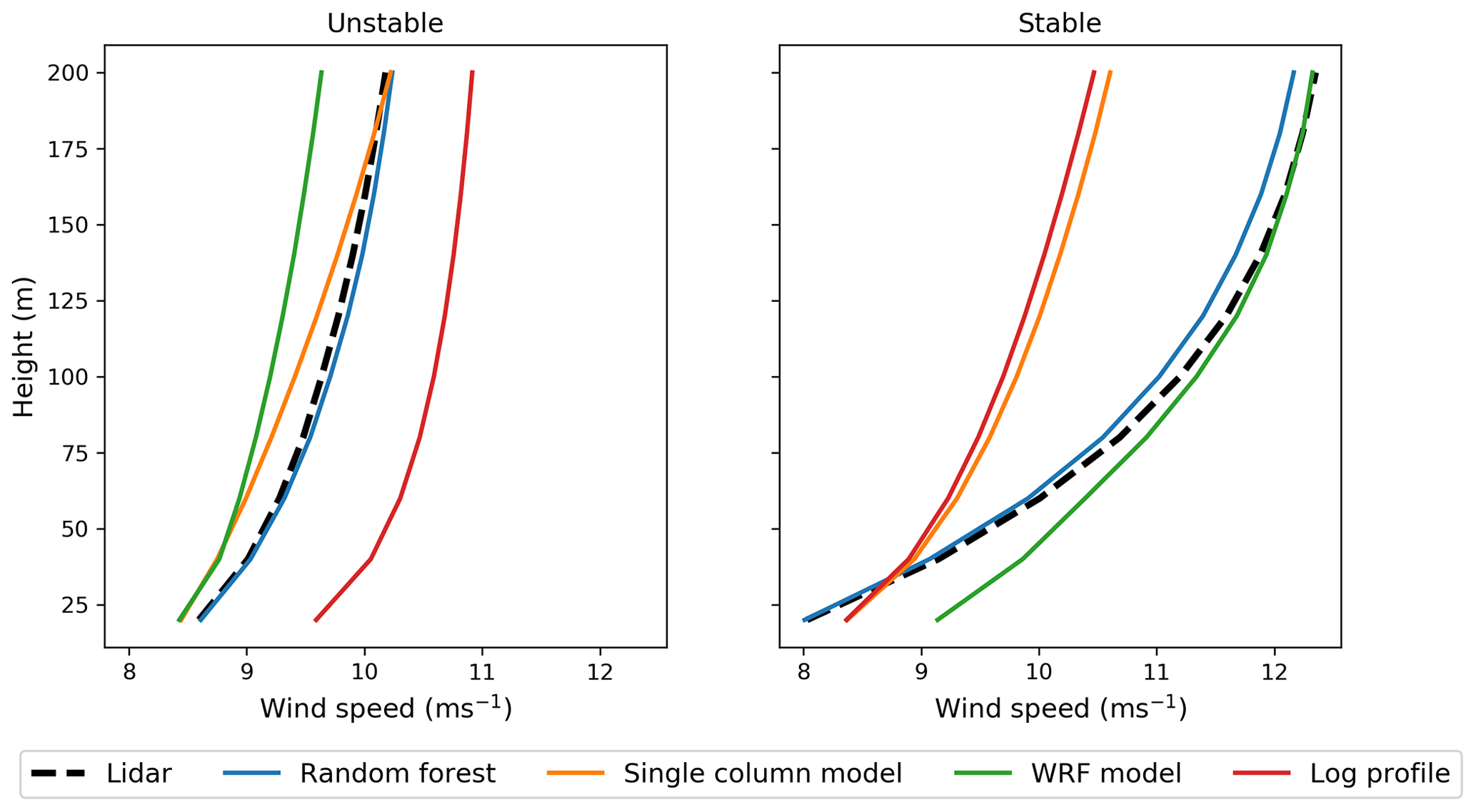
Figure 6Mean modeled and observed wind profiles at NYSERDA buoy E05 in unstable (left panels) and stable (right panels) atmospheric conditions.
This relative consistency is further illustrated in Fig. 7, which shows the REWS performance metrics by stability regime. Again, we focus on buoy E05 and note the similar relative performance between models at buoy E06. We also see the random forest with the strongest performance metrics, apart from slightly higher magnitude bias and higher EMD in stable conditions relative to the WRF model. The SCM shows lower magnitude bias and EMD in unstable relative to stable conditions but high unbiased RMSE and correlation across both regimes. The log profile performs better in unstable conditions than stable conditions for all performance metrics, whereas the WRF model cRMSE and R2 are lower in unstable conditions, but bias and EMD are higher relative to stable conditions.

Figure 7REWS performance metrics for the different vertical extrapolation models at NYSERDA buoy E05 for unstable and stable conditions.
Next, we present 12-by-24 heat maps to show the combined diurnal and monthly trends of model performance. We show only the bias heat maps in Fig. 8. We see that the machine-learning model has consistently low magnitude bias throughout the diurnal and monthly cycles, with no clear diurnal trends but a tendency to overestimate wind speeds in the fall. The SCM shows considerable negative bias throughout the year, with a tendency to overestimate wind speeds in November. Interestingly, the bias in December is positive from 01:00 to 12:00 LT and negative form 13:00 to 00:00 LT. The WRF model shows some trends, with positive bias in spring in the early hours and negative bias in the middle hours. Finally, the logarithmic profile shows substantial trends, with strong overestimation of winds through most of the year and underestimation in spring, with the largest magnitude of the underestimates in the early hours.
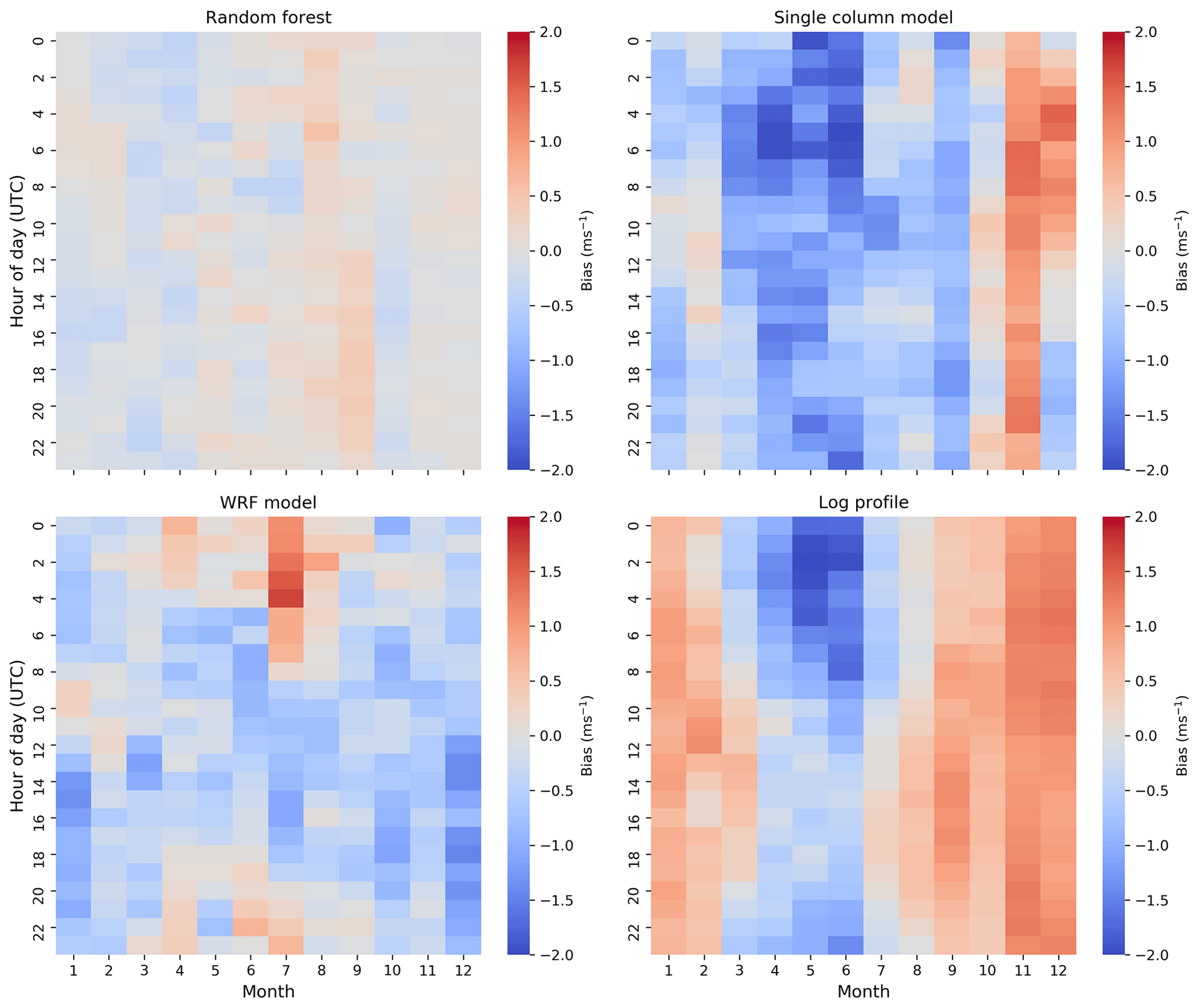
Figure 8Heat maps (12 by 24) of REWS bias at NYSERDA buoy E05 for the different extrapolation models.
4.1 Explaining DTU model performance
Figure 4 showed that the DTU method significantly overestimated wind speeds. This is a surprising result given its strong performance in Badger et al. (2015), in which 10 m satellite-measured winds were extrapolated. To explore this, we compare DTU model performance using both 2 and 20 m measurements as the basis for extrapolation. The results are shown in Fig. 9. The extrapolation from the 2 m measurements does not match the measured wind speed profile. This is likely because the measurement height is too low and located within the viscous sublayer, where log-law approximations are not valid. When the same method is used to extrapolate from the 20 m lidar measurements, we see a good match between the extrapolated and measured values. This analysis reveals that the DTU method is not suitable for extrapolation based on buoy wind speed measurements, which are often made with propeller or cup anemometers between 2 and 5 m above the sea surface. Instead, this method should be applied to short offshore meteorological masts and satellite-derived wind speed estimates.

Figure 9Mean observed and modeled wind profiles at NYSERDA buoy E05 when using the DTU method based on 2 and 20 m measurements.
4.2 Feature importance in the random forest
Finally, we examine the random forest model in more detail given its strong performance in this study. Figure 10 shows the relative feature importance for each variable used to train the random forest model. Feature importance for the random forest model is calculated based on how many times the algorithm uses the variable to split the data, weighted by the improvement in model performance because of the split. Not surprisingly, the 2 m wind speed is the most important feature (nearly 80 %). The second most important feature is the air–sea temperature difference at nearly 20 %. This is an important result and highlights the influence of atmospheric stability on offshore wind profiles.
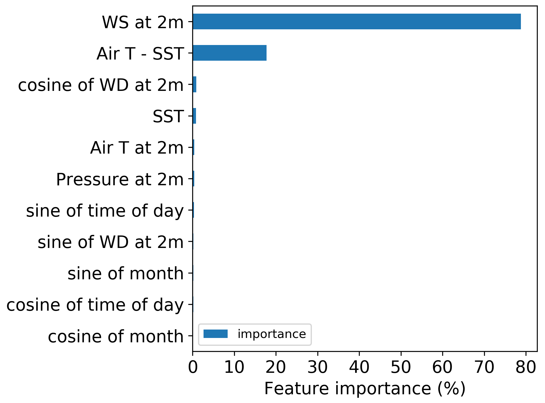
Figure 10Relative feature importance for the random forest model in predicting 120 m wind speeds at NYSERDA buoy E05.
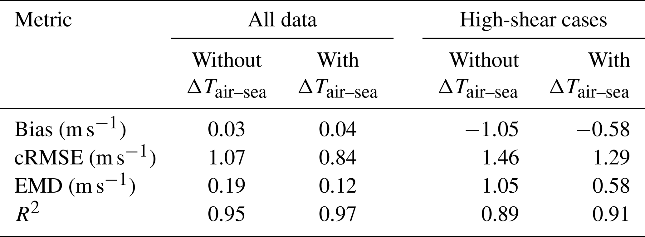
In fact, Debnath et al. (2020) found that a positive air–sea temperature difference was the key driver in the observed frequent occurrences of extreme wind shear and low-level jet events at the E05 and E06 buoys. Table 8 shows that including the air–sea temperature difference results in considerable improvements in random forest model performance, especially during the extreme high-shear cases identified in Debnath et al. (2020). Notably, the bias and EMD are both halved for the high-shear cases when using the air–sea temperature difference as an input feature.
Table 8Performance metrics at buoy E05 for the random forest model with and without the air–sea temperature difference (ΔTair–sea) as an input feature.
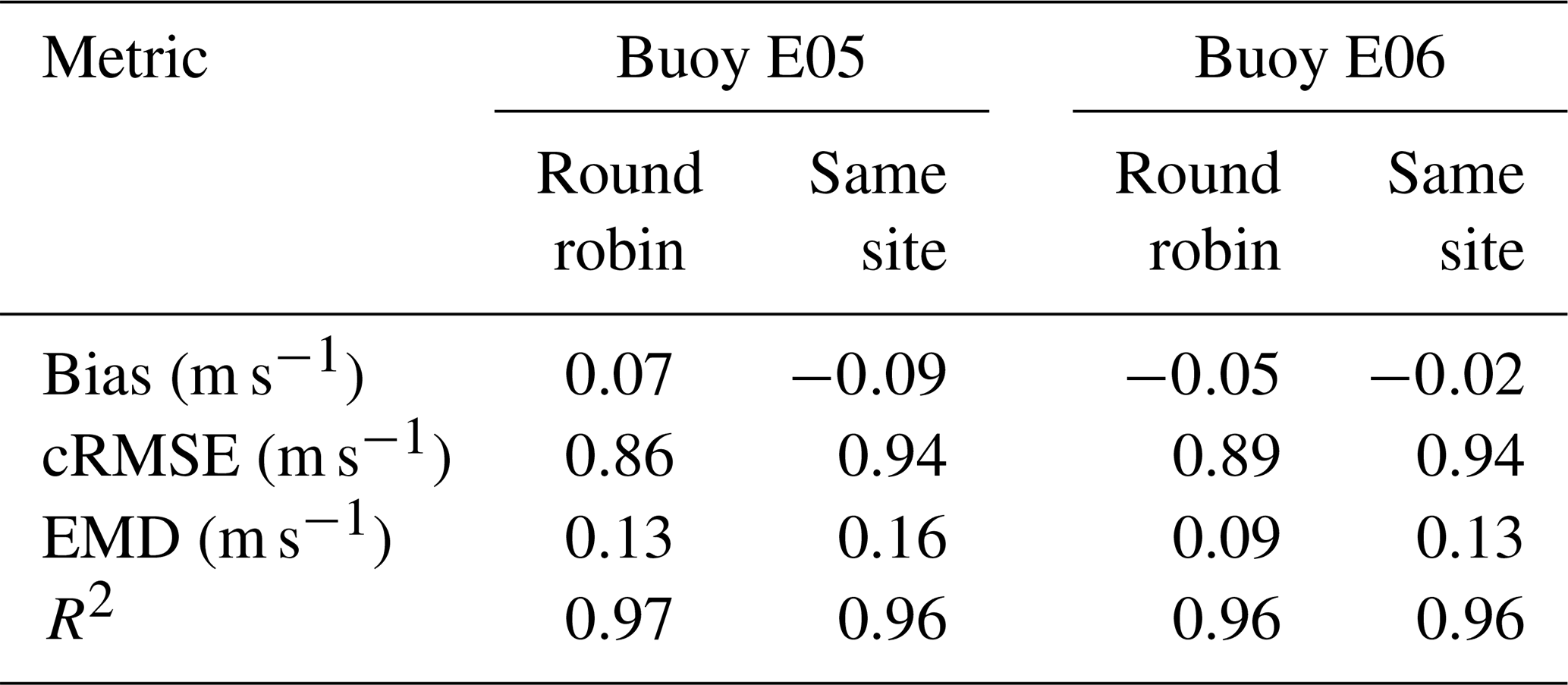
Finally, we examine how random forest model performance using the default round-robin approach (i.e., model trained and tested at different buoys) compares to that when trained and tested at the same site. In general, the model should perform best when tested at the training site, as was found in Bodini and Optis (2020b). The degree of model deterioration with distance can provide insight into how well the model can generalize across space to perform extrapolation. The results of this comparison are shown in Table 9. Interestingly, at each site and for each metric, the round-robin performance is slightly better than the same-site performance. Accounting for the fact that the limited 1-year analysis contributes to some uncertainty in these metrics, it is clear that there is at best negligible model degradation throughout an offshore distance of 83 km. In contrast, Bodini and Optis (2020b) found that, on land, model performance decreased with distance from the training site, ranging from 11 %–14 % reductions throughout distances ranging between 40–100 km. The negligible performance reduction offshore – which can be attributed to the horizontal homogeneity of the offshore environment – has important implications for the applicability of machine-learning extrapolation techniques for all US offshore waters using only a handful of lidar training sites.
Table 9Comparison of random forest model performance when trained and tested under a round-robin vs. a same-site approach.
In this study, we developed novel methods for the vertical extrapolation of near-surface offshore wind speeds. We evaluated these methods against conventional extrapolation methods and WRF-modeled wind speeds using two floating lidars deployed in US Atlantic wind energy call areas during a 1-year period. Of the four wind speed vertical extrapolation models considered, the random forest machine-learning model significantly outperformed the other models and accurately represented winds across the vertical profile in different seasons and times of day and in different stability regimes. Further, the random forest model substantially outperformed the WRF model, highlighting the benefit of local observations in generating wind profiles. Moreover, the random forest model showed negligible to no performance decrease throughout the 83 km distance between the two floating lidars.
The SCM performance offshore could be improved considerably through better accounting of near-surface stability. The model was forced at its lower boundary only by the 2 m wind speed and temperature and critically did not consider the role of sea surface temperature and related heat flux; therefore, the SCM really had no way to account for or to characterize the role of atmospheric stability, which was demonstrated in this study to be an important driver of the wind profile. In contrast, the WRF model can capture these effects, and the machine-learning model used the air–sea temperature difference, a proxy for atmospheric stability, as an input variable, which considerably improved model results. Improving the SCM design to account for atmospheric stability (e.g., by substituting the temperature lower boundary condition with a flux-based measurement) should be an area of future work.
Results from this study clearly show the promise of a machine-learning-based approach to offshore wind extrapolation. It seems likely that models trained on only a handful of lidars dispersed in offshore waters could be sufficient to accurately extrapolate wind speeds at all offshore locations in the surrounding area where surface measurements exist. This hypothesis should be tested more thoroughly using the additional floating lidars recently deployed in US waters (Table 1). The ability for a machine-learning model to generalize across different oceans in particular (e.g., training a model in the Atlantic and testing it in the Pacific) would be an important area of future work as the US offshore wind industry looks to Hawaii, the Pacific Northwest, and the Great Lakes for future expansion (Musial et al., 2020).
Applying the machine-learning approach to satellite-based wind speed observations would be the next future area of study. A collaboration between the National Renewable Energy Laboratory and DTU resulted in a US Atlantic wind atlas at 10 m a.s.l. (above sea level) (Ahsbahs et al., 2020). Training and evaluating a machine-learning model at floating lidar sites using only data available across all the US Atlantic area (i.e., satellite-measured winds and sea surface temperature) would provide key insights into whether the Ahsbahs et al. (2020) wind atlas could be accurately extrapolated across offshore wind turbine rotor-swept heights.
This proposed scope of future research will be aided by continued efforts to make floating lidar data public. Most deployed lidars are currently owned by wind energy developers and not publicly available. Public access to these data would greatly improve our understanding of the US offshore wind resource and help produce more accurate hub-height observation-based offshore wind atlases.
MO wrote the manuscript, conducted the WRF simulations, and performed the inter-model comparison. NB built the random forest model and wrote Sect. 3.3, MD built the SCM model and wrote Sect. 3.4, and PD built the DTU model and wrote Sect. 3.2.
The authors declare that they have no conflicts of interest.
This work was supported and funded by the Bureau of Ocean Energy Management. We would like to thank Angel McCoy specifically for her support and guidance throughout this work. We also thank NYSERDA and DNV-GL for making the two floating lidar data publicly available, without which this study would not have been possible.
This research has been supported by the Bureau of Ocean Energy Management (grant no. IAG-19-2122).
This paper was edited by Joachim Peinke and reviewed by two anonymous referees.
Ahsbahs, T., Badger, M., Karagali, I., and Larsén, X. G.: Validation of Sentinel-1A SAR Coastal Wind Speeds Against Scanning LiDAR, Remote Sens., 9, 552–569, https://doi.org/10.3390/rs9060552, 2017. a
Ahsbahs, T., Maclaurin, G., Draxl, C., Jackson, C. R., Monaldo, F., and Badger, M.: US East Coast synthetic aperture radar wind atlas for offshore wind energy, Wind Energ. Sci., 5, 1191–1210, https://doi.org/10.5194/wes-5-1191-2020, 2020. a, b, c
Atlantic Shores Offshore Wind: Atlantic Shores Floating LiDAR Buoy Data, available at: https://erddap.maracoos.org/erddap/tabledap/AtlanticShores_ASOW-4_wind.html (last access: 11 June 2021), 2020. a
Baas, P., Bosveld, F., Lenderink, G., van Meijgaard, E., and Holtslag, A. A. M.: How to design single-column model experiments for comparison with observed nocturnal low-level jets, Q. J. Roy. Meteorol. Soc., 136, 671–684, https://doi.org/10.1002/qj.592, 2010. a
Badger, M., Peña, A., Hahmann, A. N., Mouche, A. A., and Hasager, C. B.: Extrapolating Satellite Winds to Turbine Operating Heights, J. Appl. Meteorol. Clim., 55, 975–991, https://doi.org/10.1175/JAMC-D-15-0197.1, 2015. a, b, c, d
Beiter, P., Musial, W., Duffy, P., Cooperman, A., Shields, M., Heimiller, D., and Optis, M.: The Cost of Floating Offshore Wind Energy in California Between 2019 and 2032, NREL, Golden, Colorado, USA, https://doi.org/10.2172/1710181, 2020. a, b
Bodini, N. and Optis, M.: How accurate is a machine learning-based wind speed extrapolation under a round-robin approach?, J. Phys.: Conf. Ser., 1618, 062037, https://doi.org/10.1088/1742-6596/1618/6/062037, 2020a. a, b
Bodini, N. and Optis, M.: The importance of round-robin validation when assessing machine-learning-based vertical extrapolation of wind speeds, Wind Energ. Sci., 5, 489–501, https://doi.org/10.5194/wes-5-489-2020, 2020b. a, b, c, d, e
Carbon Trust: Carbon Trust Offshore Wind Accelerator Roadmap, Tech. rep., available at: https://prod-drupal-files.storage.googleapis.com/documents/resource/public/owa-w-uflr-updated-fl-roadmap_18102018.pdf (last access: 10 March 2021), 2018. a
Charnock, H.: Wind stress on a water surface, Q. J. Roy. Meteorol. Soc., 81, 639–640, https://doi.org/10.1002/qj.49708135027, 1955. a
Cuxart, J., Holtslag, A. A. M., Beare, R. J., Bazile, E., Beljaars, A., Cheng, A., Conangla, L., Ek, M., Freedman, F., Hamdi, R., Kerstein, A., Kitagawa, H., Lenderink, G., Lewellen, D., Mailhot, J., Mauritsen, T., Perov, V., Schayes, G., Steeneveld, G.-J., Svensson, G., Taylor, P., Weng, W., Wunsch, S., and Xu, K.-M.: Single-Column Model Intercomparison for a Stably Stratified Atmospheric Boundary Layer, Bound.-Lay. Meteorol., 118, 273–303, https://doi.org/10.1007/s10546-005-3780-1, 2006. a
Debnath, M., Doubrawa, P., Optis, M., Hawbecker, P., and Bodini, N.: Extreme Wind Shear Events in US Offshore Wind Energy Areas and the Role of Induced Stratification, Wind Energ. Sci. Discuss. [preprint], https://doi.org/10.5194/wes-2020-103, in review, 2020. a, b
DNV-GL: NYSERDA Floating LiDAR Buoy Data, available at: https://oswbuoysny.resourcepanorama.dnvgl.com/ (last access: 28 February 2021), 2020. a, b, c, d
Doubrawa, P., Barthelmie, R. J., Pryor, S. C., Hasager, C. B., Badger, M., and Karagali, I.: Satellite winds as a tool for offshore wind resource assessment: The Great Lakes Wind Atlas, Remote Sens. Environ. 168, 349–359, https://doi.org/10.1016/j.rse.2015.07.008, 2015. a, b
Emeis, S.: Wind Energy Meteorology, Springer, Dordrecht, 2013. a
Hasager, C. B., Madsen, P. H., Giebel, G., Réthoré, P.-E., Hansen, K. S., Badger, J., Pena Diaz, A., Volker, P., Badger, M., Karagali, I., Cutululis, N. A., Maule, P., Schepers, G., Wiggelinkhuizen, J., Cantero, E., Waldl, I., Anaya-Lara, O., Attya, A. B., Svendsen, H., Palomares, A., Palma, J., Gomes, V. C., Gottschall, J., Wolken-Möhlmann, G., Bastigkeit, I., Beck, H., Trujillo, J.-J., Barthelmie, R., Sieros, G., Chaviaropoulos, T., Vincent, P., Husson, R., and Prospathopoulos, J.: Design tool for offshore wind farm cluster planning, in: Proceedings of the EWEA Annual Event and Exhibition 2015, EWEA – European Wind Energy Association, Paris, France, 2015. a
Hasager, C. B., Hahmann, A. N., Ahsbahs, T., Karagali, I., Sile, T., Badger, M., and Mann, J.: Europe's offshore winds assessed with synthetic aperture radar, ASCAT and WRF, Wind Energ. Sci., 5, 375–390, https://doi.org/10.5194/wes-5-375-2020, 2020. a, b
Holtslag, A. A. M.: Estimates of diabatic wind speed profiles from near-surface weather observations, Bound.-Lay. Meteorol., 29, 225–250, https://doi.org/10.1007/BF00119790, 1984. a
Jiménez, P. A., Dudhia, J., González-Rouco, J. F., Navarro, J., Montávez, J. P., and García-Bustamante, E.: A Revised Scheme for the WRF Surface Layer Formulation, Mon. Weather Rev., 140, 898–918, https://doi.org/10.1175/MWR-D-11-00056.1, 2012. a, b
Jong, P., Dargaville, R., Silver, J., Utembe, S., Kiperstok, A., and Torres, E. A.: Forecasting high proportions of wind energy supplying the Brazilian Northeast electricity grid, Appl. Energy, 195, 538–555, https://doi.org/10.1016/j.apenergy.2017.03.058, 2017. a
Kelly, M. and Gryning, S.-E.: Long-Term Mean Wind Profiles Based on Similarity Theory, Bound.-Lay. Meteorol., 136, 377–390, https://doi.org/10.1007/s10546-010-9509-9, 2010. a, b, c
Mahoney, W. P., Parks, K., Wiener, G., Liu, Y., Myers, W. L., Sun, J., Delle Monache, L., Hopson, T., Johnson, D., and Haupt, S. E.: A Wind Power Forecasting System to Optimize Grid Integration, IEEE T. Sustain. Energ., 3, 670–682, https://doi.org/10.1109/TSTE.2012.2201758, 2012. a
Mayflower Offshore Wind: Mayflower Floating LiDAR Buoy Data, available at: http://www.neracoos.org/erddap/tabledap/SHELL_MAYFLOWER_winds_csv_all.html (last access: 15 February 2021), 2020. a
Mohandes, M. A. and Rehman, S.: Wind speed extrapolation using machine learning methods and LiDAR measurements, IEEE Access, 6, 77634–77642, https://doi.org/10.1109/ACCESS.2018.2883677, 2018. a
Monin, A. and Obukhov, A.: Basic Laws of Turbulent Mixing in the Surface Layer of the Atmosphere, Contrib. Geophys. Inst. Acad. Sci., 24, 163–187, 1954. a
Musial, W., Beiter, P., Nunemaker, J., Gevorgian, V., Cooperman, A., Hammond, R., Shields, M., and Spitsen, P.: 2019 Offshore Wind Technology Data Update, Tech. Rep. NREL/TP-5000-77411, 1677477, MainId:26357, NREL, Golden, Colorado, USA, https://doi.org/10.2172/1677477, 2020. a, b
National Data Buoy Center: Meteorological and oceanographic data collected from the National Data Buoy Center Coastal-Marine Automated Network (C-MAN) and moored (weather) buoys, available at: https://www.ndbc.noaa.gov/ (last access: 10 February 2021), 1971. a
NYSERDA: Hudson North and Hudson South Call Areas Offshore Wind Farm Energy Assessment Report, Tech. rep., available at: https://oswbuoysny.resourcepanorama.dnvgl.com/, last access: 15 March 2021. a
Optis, M. and Monahan, A.: The Extrapolation of Near-Surface Wind Speeds under Stable Stratification Using an Equilibrium-Based Single-Column Model Approach, J. Appl. Meteorol. Clim. 55, 923–943, https://doi.org/10.1175/JAMC-D-15-0075.1, 2016. a, b, c
Optis, M. and Monahan, A.: A Comparison of Equilibrium and Time-Evolving Approaches to Modeling the Wind Profile under Stable Stratification, J. of Appl. Meteorol. Clim., 56, 1365–1382, https://doi.org/10.1175/JAMC-D-16-0324.1, 2017. a, b, c, d
Optis, M. and Perr-Sauer, J.: The importance of atmospheric turbulence and stability in machine-learning models of wind farm power production, Renew. Sustain. Energ. Rev., 112, 27–41, https://doi.org/10.1016/j.rser.2019.05.031, 2019. a
Optis, M., Monahan, A., and Bosveld, F. C.: Moving Beyond Monin–Obukhov Similarity Theory in Modelling Wind-Speed Profiles in the Lower Atmospheric Boundary Layer under Stable Stratification, Bound.-Lay. Meteorol., 153, 497–514, https://doi.org/10.1007/s10546-014-9953-z, 2014. a
Optis, M., Monahan, A., and Bosveld, F. C.: Limitations and breakdown of Monin–Obukhov similarity theory for wind profile extrapolation under stable stratification, Wind Energy, 19, 1053–1072, https://doi.org/10.1002/we.1883, 2016. a
Optis, M., Bodini, N., Debnath, M., and Doubrawa, P.: Best Practices for the Validation of U.S. Offshore Wind Resource Models, Tech. Rep. NREL/TP-5000-XXXXX, NREL – National Renewable Energy Laboratory, Golden, CO, USA, 2020a. a, b
Optis, M., Kumler, A., Scott, G., Debnath, M., and Moriarty, P.: Validation of RU-WRF, the Custom Atmospheric Mesoscale Model of the Rutgers Center for Ocean Observing Leadership, report no. NREL/TP-5000-75209, NREL, Golden, Colorado, USA, p. 61, https://doi.org/10.2172/1599576, 2020b. a
Optis, M., Rybchuk, O., Bodini, N., Rossol, M., and Musial, W.: 2020 Offshore Wind Resource Assessment for the California Pacific Outer Continental Shelf, Tech. Rep. NREL/TP-5000-77642, NREL – National Renewable Energy Laboratory, Golden, CO, USA, https://doi.org/10.2172/1677466, 2020c. a
Pacific Northwest National Laboratory: Buoy Lidar Data, California, available at: https://a2e.energy.gov/data?ProjectFilter=["buoy"5D] (last access: 10 May 2021), 2020. a, b
Pedregosa, F., Varoquaux, G., Gramfort, A., Michel, V., Thirion, B., Grisel, O., Blondel, M., Prettenhofer, P., Weiss, R., Dubourg, V., Vanderplas, J., Passos, A., Cournapeau, D., Brucher, M., Perrot, M., and Duchesnay, E.: Scikit-learn: Machine Learning in Python, J. Mach. Learn. Res., 12, 2825–2830, 2011. a
Skamarock, C., Klemp, B., Dudhia, J., Gill, O., Liu, Z., Berner, J., Wang, W., Powers, G., Duda, G., Barker, D., and Huang, X.-Y.: A Description of the Advanced Research WRF Model Version 4, NCAR, Boulder, Colorado, USA, https://doi.org/10.5065/1dfh-6p97, 2019. a
Smith, R. N. B.: A scheme for predicting layer clouds and their water content in a general circulation model, Q. J. Royal Meteorol. Soc., 116, 435–460, https://doi.org/10.1002/qj.49711649210, 1990. a, b
Troen, I. and Petersen, E.: European Wind Atlas, Riso National Laboratory, Roskilde, 1989. a
Vassallo, D., Krishnamurthy, R., and Fernando, H. J. S.: Decreasing wind speed extrapolation error via domain-specific feature extraction and selection, Wind Energ. Sci., 5, 959–975, https://doi.org/10.5194/wes-5-959-2020, 2020. a
Wagner, R., Cañadillas, B., Clifton, A., Feeney, S., Nygaard, N., Poodt, M., Martin, C. S., Tüxen, E., and Wagenaar, J. W.: Rotor equivalent wind speed for power curve measurement – comparative exercise for IEA Wind Annex 32, J. Phys.: Conf. Ser., 524, 012108, https://doi.org/10.1088/1742-6596/524/1/012108, 2014. a
Wang, Y.-H., Walter, R. K., White, C., Farr, H., and Ruttenberg, B. I.: Assessment of surface wind datasets for estimating offshore wind energy along the Central California Coast, Renew. Energy, 133, 343–353, https://doi.org/10.1016/j.renene.2018.10.008, 2019. a
Both are needed because each value of sine only (or cosine only) is linked to two different values of the cyclical feature.