Comparing and validating intra-farm and farm-to-farm wakes across different mesoscale and high-resolution wake models

Numerical wind resource modelling across scales from the mesoscale to the turbine scale is of increasing interest due to the expansion of offshore wind energy. Offshore wind farm wakes can last several tens of kilometres downstream and thus affect the wind resources of a large area. So far, scale-specific models have been developed but it remains unclear how well the different model types can represent intra-farm wakes, farm-to-farm wakes as well as the wake recovery behind a farm. Thus, in the present analysis the simulation of a set of wind farm models of different complexity, fidelity, scale and computational costs are compared among each other and with SCADA data. In particular, two mesoscale wind farm parameterizations implemented in the mesoscale Weather Research and Forecasting model (WRF), the Explicit Wake Parameterization (EWP) and the Wind Farm Parameterization (FIT), two different high-resolution RANS simulations using PyWakeEllipSys equipped with an actuator disk model, and three rapid engineering wake models from the PyWake suite are selected. The models are applied to the Nysted and Rødsand II wind farms, which are located in the Fehmarn Belt in the Baltic Sea.

Based on the performed simulations, we can conclude that both WRF + FIT (BIAS = 0.52 m s⁻¹) and WRF + EWP (BIAS = 0.73 m s⁻¹) compare well with wind farm affected mast measurements. Compared with the RANS simulations, baseline intra-farm variability, i.e. the wind speed deficit in between turbines, can be captured reasonably well with WRF + FIT using a resolution of 2 km, a typical resolution of mesoscale models for wind energy applications, while WRF + EWP underestimates wind speed deficits. However, both parameterizations can be used to estimate median wind resource reduction caused by an upstream farm. All considered engineering wake models from the PyWake suite simulate peak intra-farm wakes comparable to the high fidelity RANS simulations. However, they considerably underestimate the farm wake effect of an upstream farm although with different magnitudes. Overall, the higher computational costs of PyWakeEllipSys and WRF compared with those of PyWake pay off in terms of accuracy for situations when farm-to-farm wakes are important.

1 Introduction

Numerical wind resource modelling for wind energy covers scales from the wind turbine level to the meso- and macroscale of synoptic systems (Fig. 1; Porté-Agel et al., 2020; Veers et al., 2019). In the past, targeted models have been developed for the different scales. However, with the increasing expansion of wind energy, atmospheric processes that involve different scales are of increasing relevance: individual microscale wind turbine wakes converge to a wind farm wake downstream of a farm. These wind farm wakes can extend more than 50 km both onshore (Lundquist et al., 2019) and offshore (Cañadillas et al., 2020) and thus affect wind resources of neighbouring farms. In addition, they are affected by processes on the mesoscale and synoptic scale, which become increasingly relevant as the studied area becomes larger (Vincent et al., 2013; Mehrens et al., 2016); thus, flow over larger areas is not uniform. Rapid engineering models or other high-resolution models that are targeted for the use of microscales around turbines often do not account for this non-uniformity. Instead mesoscale models equipped with a wind farm parameterization (WFP) can be applied to capture these mesoscale variabilities. However, with a typical resolution of about 1–2 km used in wind energy applications according to Fischereit et al. (2022), mesoscale models cannot resolve individual turbines within a farm.

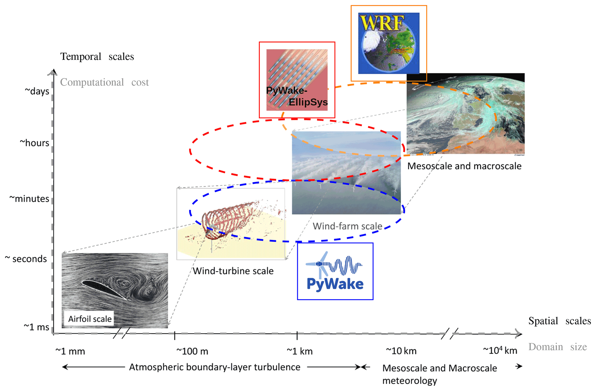
Figure 1 Scales relevant for wind energy and targeted models with their associated resolution and computational costs. Taken from Porté-Agel et al. (2020) in accordance with the Creative Commons Attribution (CC BY) license with modifications.

With this in mind, the aim of this study is 2-fold: first, to evaluate the performance of WFPs included in a mesoscale model using a typical horizontal resolution applied in wind energy application against mast measurements, SCADA data and high-resolution wake models, sometimes also termed wind turbine wake models (Göçmen et al., 2016), in terms of intra-farm wakes; and second, to compare farm-to-farm wakes and long-distance wakes of WFPs and high-resolution wake models. Different model types do not only differ in the typical domain size and therefore in the spatial scales that they can capture, but also by their computational costs measured in central processing unit (CPU) time (Fig. 1). Thus, based on the analysis this study also addresses the question of whether more computational demanding model simulations provide better accuracy when modelling intra-farm and farm-to-farm wakes.

For the investigations, we employ as the mesoscale model the Weather Research and Forecasting (WRF) v4.2.2 model (Skamarock et al., 2019) equipped with the Explicit Wake Parameterization (EWP, Volker et al., 2015) and the wind farm parameterization by Fitch et al. (2012) (FIT). FIT and EWP are the most applied WFPs according to a recent review (Fischereit et al., 2022). While some studies have investigated intra-farm wakes using FIT (Jiménez et al., 2015; Eriksson et al., 2015, 2017), only a few studies (Hansen et al., 2015; Poulsen, 2019) have evaluated intra-farm wakes with EWP against measurements or SCADA data. In addition, in Hansen et al. (2015) WRF was used in a very coarse horizontal resolution so that the entire wind farm was located within one grid cell. In contrast to that, Jiménez et al. (2015) and Eriksson et al. (2015) used WRF with a very high horizontal resolution of 333 m and Eriksson et al. (2017) even a resolution of 111 m. These resolutions are within the terra incognita numerical region or the “grey” zone of the applicability of mesoscale models (Wyngaard, 2004; Honnert et al., 2020). Within that zone, large coherent overturning structures start to be partially resolved when their length scale is approaching the effective grid resolution. This violates assumptions that are applied in the turbulence and shallow convection parameterizations and thus reduces the accuracy of the numerical simulations in that zone (Honnert et al., 2020). In the present study, a typical resolution for wind energy applications (Fischereit et al., 2022), namely 2 km, is applied.

The intra-farm wakes in WRF–EWP and WRF–FIT are evaluated both against SCADA data as well as high-resolution Computational Fluid Dynamics Reynolds-Averaged Navier–Stokes (CFD–RANS) and engineering wake modelling. We employ the RANS model PyWakeEllipSys (PyWakeEllipSys, 2022), which is based on the EllipSys3D CFD flow solver (Michelsen, 1992; Sørensen, 1995) and three different engineering wake models included in the PyWake suite (Pedersen et al., 2019). High-resolution wake models are typically applied to single wind farms. Only a few studies have applied engineering wake models to farm-to-farm cases (Nygaard and Hansen, 2016; Nygaard et al., 2020; Larsén et al., 2019) or to evaluate long-distance wakes (Nygaard and Newcombe, 2018). These studies found that simple wake models can in principle represent farm-to-farm wakes if no coastal gradient is present, but did not compare the performance of different engineering wake models, which will be done in this study.

The paper is structured as follows: in Sect. 2 the applied mesoscale and high-resolution wake models as well as the available measurements are introduced. The results are presented in Sect. 3 and split into two parts. In the first part, WRF simulation results are evaluated against mast measurements (Sect. 3.1). In the second part, the performance of the different wake models to represent intra-farm (Sect. 3.2) and farm-to-farm wakes (Sect. 3.3) is evaluated for a flow case including farm-to-farm effects. In addition, the representation of the global blockage effect upstream of a wind farm in the different models is briefly compared in Sect. 3.4. The results are summarized and discussed in Sect. 4.

Table 1 Characteristics of simulated wind farms in Fig. 2.

2 Method

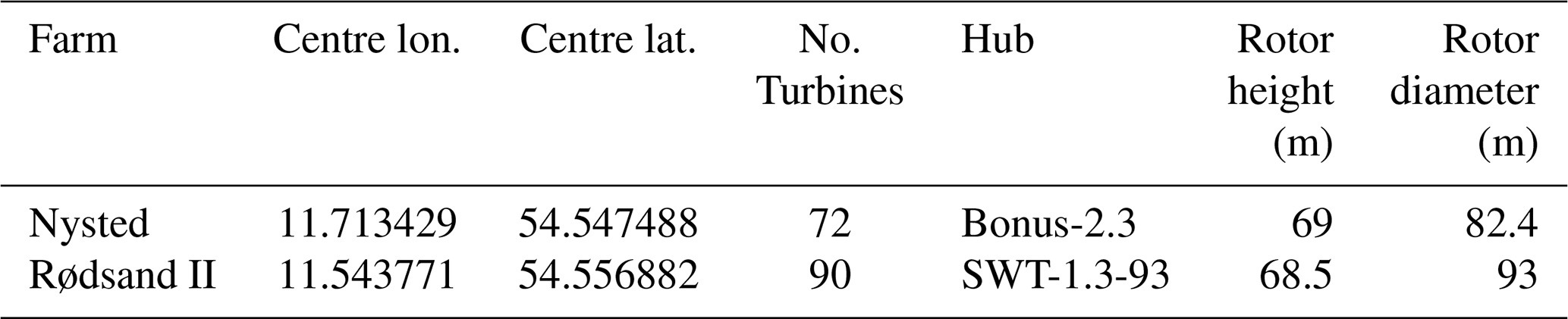
The Fehmarn Belt with the wind farms Nysted (abbreviated NY herein) and Rødsand II (abbreviated RØ herein) has been selected as the study area (Fig. 2). This area was chosen since it offers the opportunity to study farm-to-farm effects between Nysted and Rødsand II and mast measurements, and supervisory control and data acquisition (SCADA) control system data for Rødsand II wind farm were available for evaluation. Details on the two wind farms are given in Table 1. Power, thrust and rotational speed curves of the two wind turbine models are shown in Fig. 3. Note that the rotor speed is only used for the PyWakeEllipSys RANS–AD simulations where it influences the shape of the thrust and tangential force distributions, and it defines the magnitude of the tangential force that induces wake rotation (see Sect. 2.2.1 for more details). The curve of the rotor speed in Fig. 3 is simplified for the present analysis. In reality the Bonus wind turbine shows a hysteresis behaviour between 5 and 7 m s⁻¹: approaching this region from lower wind speeds, the rotor speed is kept at the minimum value of 11 rpm, while approaching from higher wind speeds the maximum value of 16.5 rpm is kept, as explained in Nygaard and Hansen (2016). Thus, the linear interpolation between the two rotor speeds between 7 and 8 m s⁻¹, as used in this study, is a simplification. However, since we focus on Rødsand II and not on Nysted for the detailed analysis of internal wakes, this will not strongly influence the results. In addition, the effect of wake rotation on the velocity deficit (which induces a small wake deflection when combined with a wind shear) is small under neutral conditions (van der Laan et al., 2015a). More details on the available observations are given in Sect. 2.1; the applied models and their setups are described in Sect. 2.2.

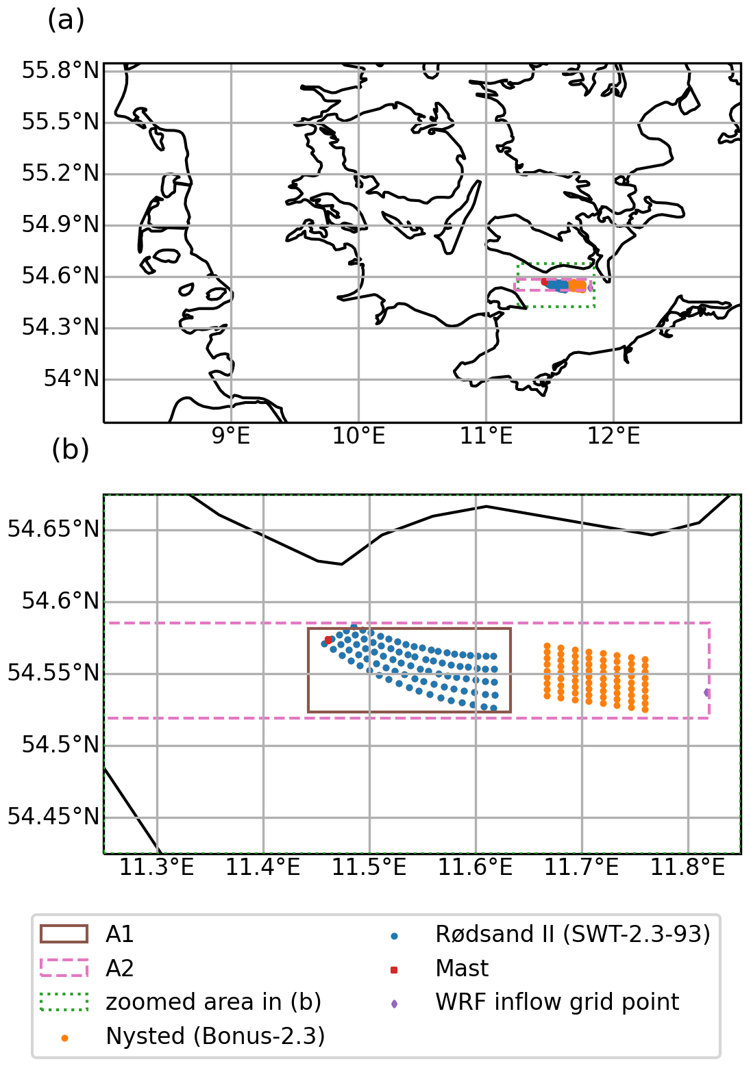
Figure 2 The study area, Fehmarn Belt, with wind farms and mast location. Panel (b) is a zoom of the dotted green area in (a). The dot in the east refers to the WRF grid point used for the filtering in Sect. 2.2.3. The solid and dashed rectangles A1 and A2 are used for the analysis of the farm-to-farm wake effect in Fig. 15. Details of the wind farms are given in Table 1.

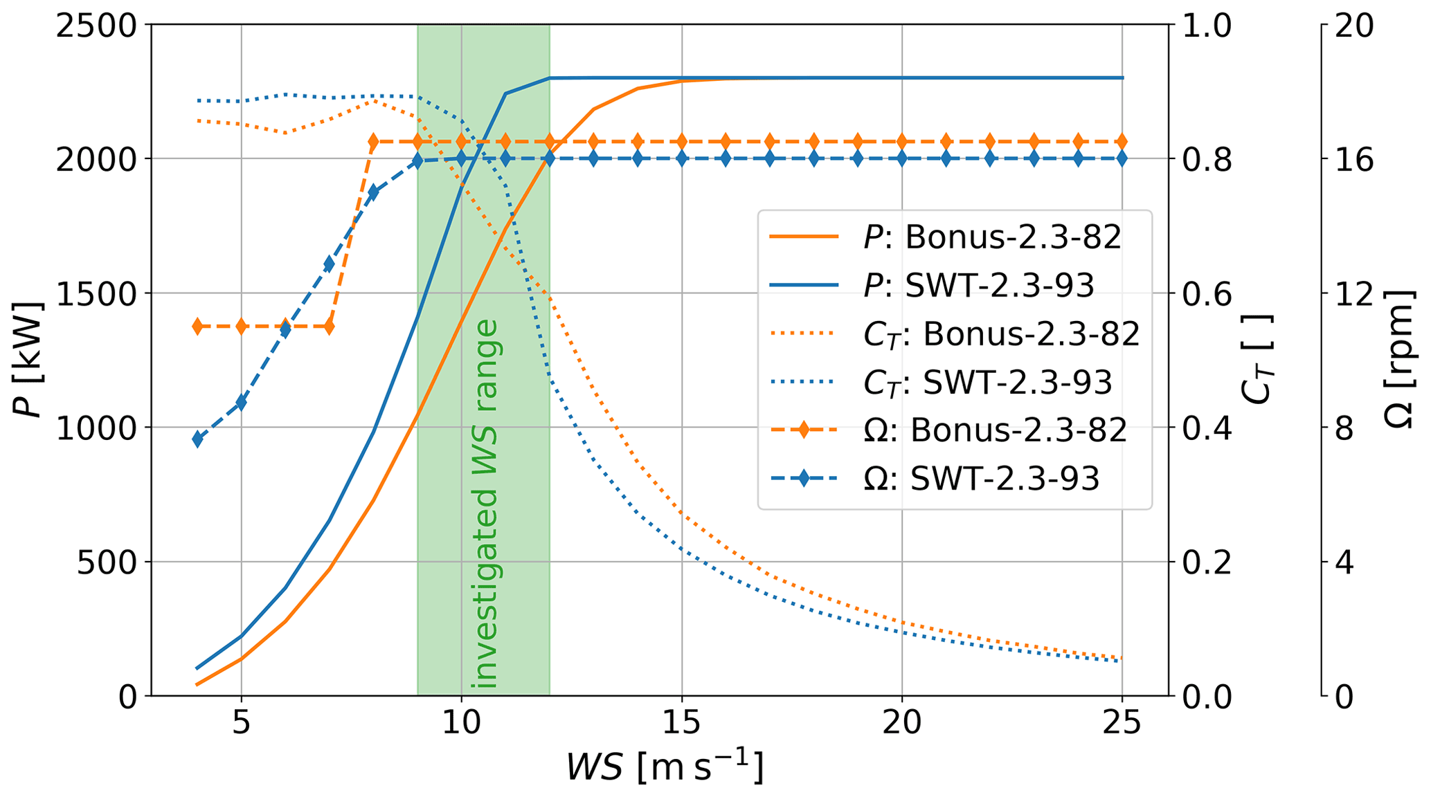
Figure 3 Power (P, left axis), thrust curve (C_T, right axis) and rotor speed (Ω, rightmost axis) for the two turbine models of this study. The shaded green area indicates the investigated wind speed range in this study.

2.1 Measurements

Wind measurements with sonic anemometers at three heights (Table 2) are available from a mast located at the western side of Rødsand II (red dot in Fig. 2). Sonic anemometers also measure air temperature, T, which is used to derive the Obukhov length, L, based on Lange et al. (2004) in the following way:

$$\begin{array}{}\text{(1)}& L={\displaystyle \frac{-T\cdot {\left(u_{*}\right)}^{\mathrm{3}}}{\mathrm{9.81}\cdot \mathrm{0.4}\cdot \stackrel{\mathrm{‾}}{w^{\prime }{T}^{\prime }}}}.\end{array}$$

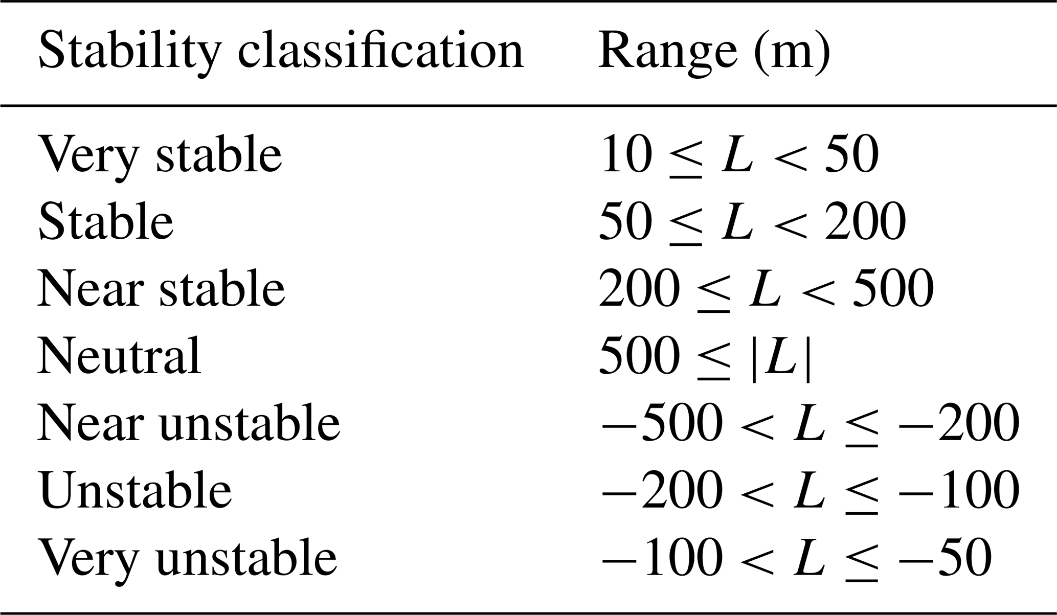
This characterizes the stability conditions. Here, $\stackrel{\mathrm{‾}}{w^{\prime }{T}^{\prime }}$ is the covariance of vertical wind speed and temperature fluctuations and u_* is the friction velocity, which is derived from the sonic signals. All values are taken from the measurements at 57 m height. Based on the derived value for L, stability is classified according to Table 3, which has been taken from Hansen et al. (2012).

Table 2 Available instruments and periods for the mast (red dot in Fig. 2) and SCADA data of Rødsand II.

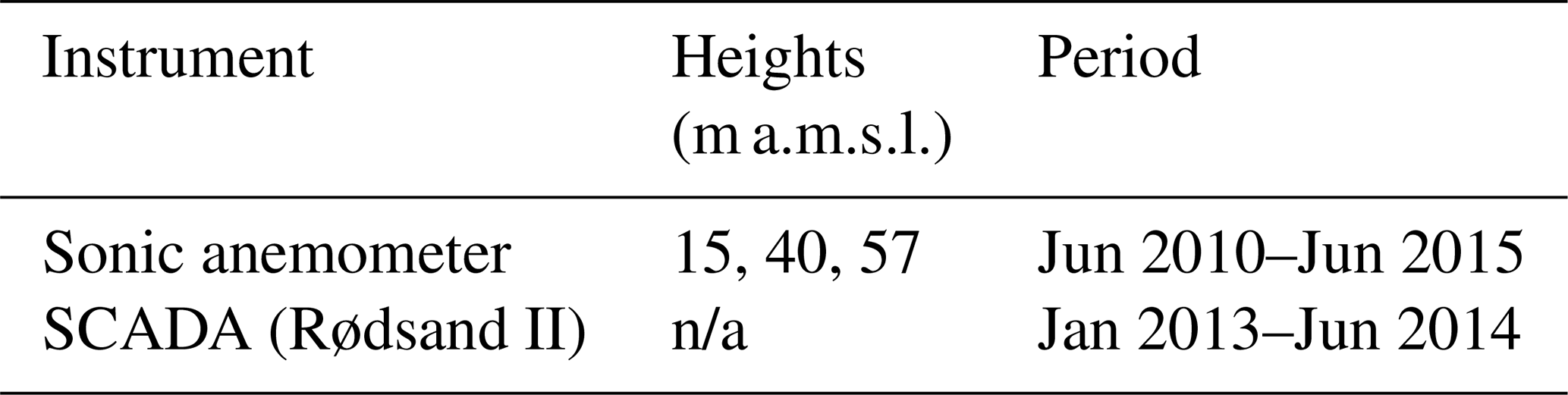
n/a: not applicable.

Table 3 Stability classification based on the Obukhov length, L (m), derived from Eq. (1).

In addition, 10 min SCADA data is available for all 90 turbines of Rødsand II from January 2013 until the end of June 2014. The SCADA data include electric power, rotor speed, yaw position and nacelle wind speed. The SCADA data has been quality controlled (Hansen et al., 2015). From the SCADA data, the equivalent wind turbine wind speed was derived from the 10 min values of the power combined with the power curve below rated power. During October 2013, mast measurements were available 88 % of the time and SCADA data were available 100 %. Therefore, this period has been chosen for this study. Since no SCADA data for the turbines of Nysted were available, we assume for this study that Nysted was online and operated with 100 % capacity during that period following the discussion in Hansen et al. (2015).

2.2 Applied models and setups

Three different types of models are employed in this study. The models and setups are described for the CFD–RANS model from PyWakeEllipSys in Sect. 2.2.1, for the engineering wake model suite PyWake in Sect. 2.2.2 and for the mesoscale model WRF in Sect. 2.2.3.

2.2.1 CFD–RANS wake modelling using PyWakeEllipSys

We apply the RANS model from PyWakeEllipSys v1.5.1 (PyWakeEllipSys, 2022), which is based on the EllipSys3D CFD flow solver initially developed by Michelsen (1992) and Sørensen (1995). EllipSys3D is an incompressible finite volume flow solver using a block-structured grid. PyWakeEllipSys is developed to simulate the wind turbine interaction subjected to an atmospheric inflow that can represent effects of turbulence intensity (TI), atmospheric stability, ABL height and Coriolis forces (van der Laan et al., 2021a). The inflow models are all based on modified k–ε turbulence model closures.

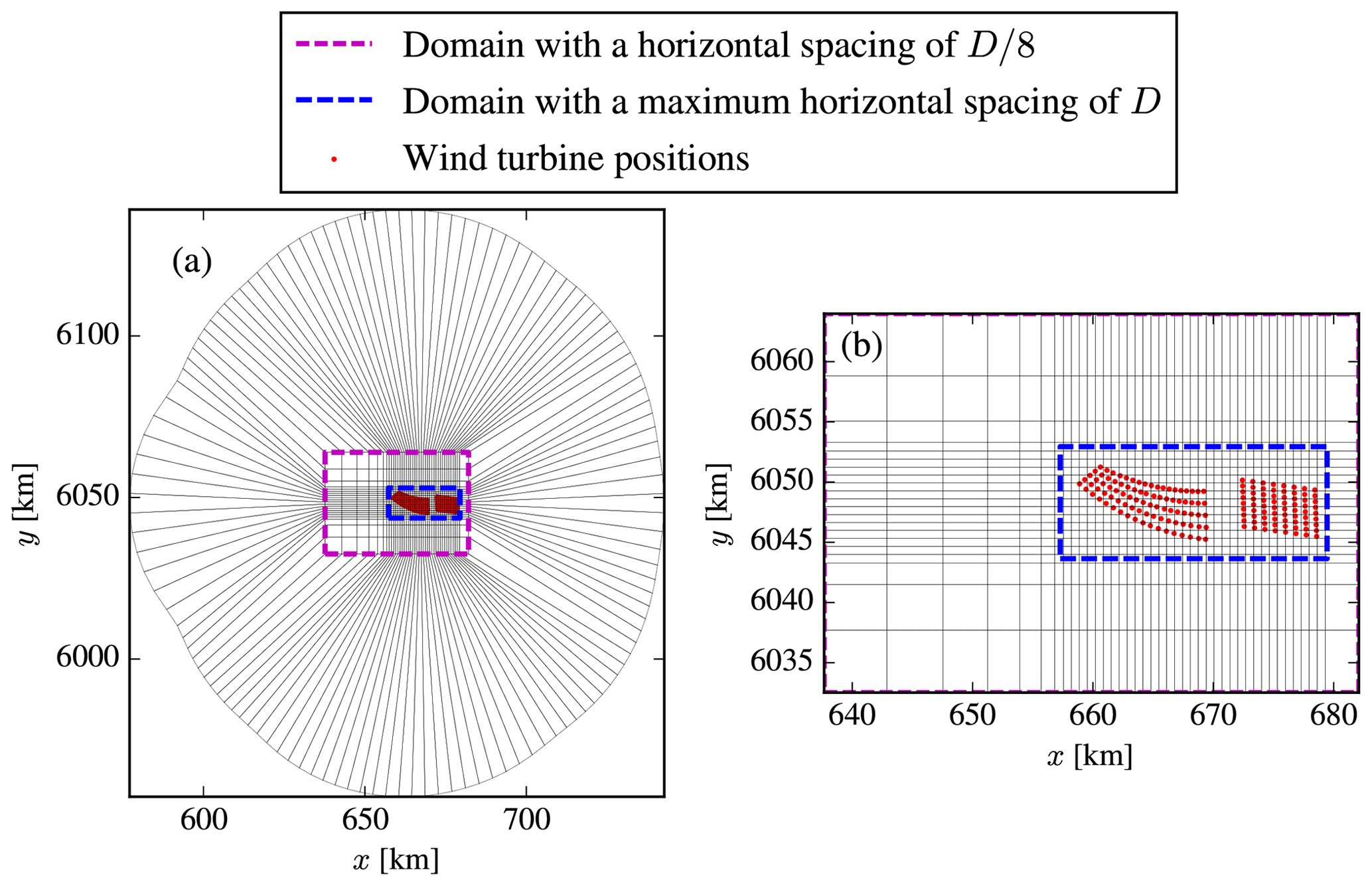
Figure 4 Surface grid of RANS simulations where every 64th grid line is shown. Two inner regions are marked by the magenta and blue dashed boxes. Wind farm layouts are shown as red dots. Panel (b) is a zoomed view of (a).

The numerical domain represents an o-grid of about 160 km in diameter and has two nested refined inner regions, as depicted in Fig. 4. The innermost region (dashed blue box in Fig. 4) has uniform spacing in the horizontal directions using a cell size of $D/\mathrm{8}$, based on a grid refinement study from van der Laan et al. (2015b), where D is the rotor diameter of the Bonus-2.3 wind turbine. The outer refinement region (dashed magenta box in Fig. 4) is used to resolve the wind farm wake using a maximum horizontal spacing of 1 D. The first cell height is set to 1.5 m and grows initially to $D/\mathrm{8}$ at a height of 3 D, and then continues to grow upwards until a domain height of 25D is reached. In total 258 million cells are used. A rough wall boundary condition (Sørensen et al., 2007) is set as the ground and an inflow condition is used at the top of the domain. The lateral boundaries are either inflow or outflow boundaries depending on the inflow wind direction. The outflow boundary has an angle of 45^∘, at which all gradients normal to the boundary are assumed to be zero.

We have chosen to employ two inflow models: a pure neutral inflow following a logarithmic profile and a near-neutral inflow including an ABL height and Coriolis forces. The models are referred to as k–ε and k–ε ABLc in van der Laan et al. (2021a), respectively, where more information can be found. In the present work, we use RANS–ASL and RANS–ABL to distinguish the k–ε and k–ε ABLc models, respectively. The employed inflow profiles are depicted in Fig. 5. The RANS–ASL model represents a neutral surface layer and only has the roughness length as an input parameter, which we set as $\mathrm{9.33}\times {\mathrm{10}}^{-\mathrm{4}}$ m to get a TI of 7 % at hub height. The TI value of 7 % was chosen based on a directional analysis of measured streamwise TI, from cup anemometers of 48 m height at the Rødsand II mast for the period November 2002–June 2005, i.e. before the installation of Rødsand II (Fig. 6). Differences in TI between sectors are visible, reflecting landward and seaward sectors (Fig. 2). For easterly wind, a streamwise TI of 10.4 % is estimated. This value is likely influenced by the presence of Nysted. The closest seaward sector, 120^∘, has a streamwise TI of about 7 %. Converting both streamwise TI values, TI_u, to total TI using the approach by Panofsky and Dutton (1984), $\mathrm{TI}=\sqrt{\mathrm{1}/\mathrm{3}\left(\mathrm{1}+{\mathrm{0.8}}^{\mathrm{2}}+{\mathrm{0.5}}^{\mathrm{2}}\right)}{\mathrm{TI}}_{\mathrm{u}}$, one arrives at 8 % and 6 %, respectively. These values are very similar to the TI value of 7 % chosen in Hansen et al. (2015) for wind speeds around 8 m s⁻¹; thus, 7 % has been chosen here for simplicity. A slight sensitivity of the results to the chosen TI value can be expected.

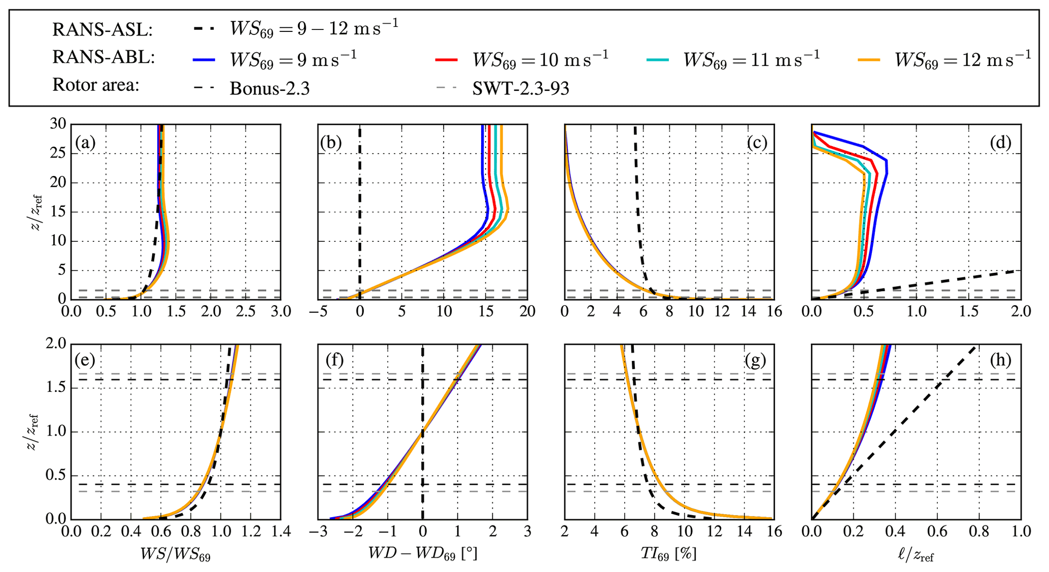
Figure 5 Inflow profiles for RANS simulations. Panels (e–h) are a zoomed view of (a–d), focused around wind turbine rotor areas, which are depicted as black (Bonus-2.3) and grey (SWT-2.3-93) dashed lines. (a, e) Wind speed (WS); (b, f) wind direction (WD); (c, g) turbulence intensity (TI); and (d, h) turbulence length scale (ℓ).

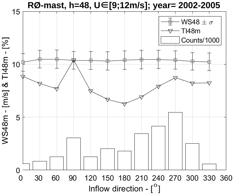
Figure 6 Streamwise TI and mean wind speed at 48 m height for different wind directions from measurements filtered for a wind speed range of 9–12 m s⁻¹.

The friction velocity is used to scale the inflow profile to get the desired hub height wind speed, and its value is found by a one-dimensional precursor simulation that includes the same numerical errors close to the wall as the 3D wind farm simulation, although the shape of the resulting profile is very similar to the analytical logarithmic profile. The use of one-dimensional inflow precursor assures that the inflow is in full balance with the three-dimensional domain, which is a requirement to investigate small effects as wind farm blockage. The RANS–ABL model represents an ABL height by setting a maximum turbulence length scale, ℓ_max following Apsley and Castro (1997). For small values of ℓ_max, a shallow ABL height is obtained and the resulting ABL profiles resemble stable conditions, without the need for a temperature equation. We choose a roughness length of $\mathrm{5}\times {\mathrm{10}}^{-\mathrm{3}}$ m and set the Coriolis parameter to $\mathrm{1.187}\times {\mathrm{10}}^{-\mathrm{4}}$ s⁻¹ corresponding to a latitude of 54.5^∘. A pre-calculated ABL library using Rossby similarity (van der Laan et al., 2021b) is used to find the geostrophic wind speed G and ℓ_max that sets the desired turbulence intensity and wind speed at the reference height of 69 m. Four wind speeds at hub height are employed (WS₆₉), namely 9, 10, 11 and 12 m s⁻¹ (see Sect. 2.3.1), and we find G=11.3, 12.8, 14.3 and 15.8 m s⁻¹ and ℓ_max=38.3, 34.9, 32.3 and 30.3 m, respectively. The obtained values of ℓ_max can be related to the Obukhov length as $L\approx {\mathrm{\ell }}_{\max }/\mathrm{0.08}$, following Apsley and Castro (1997), which gives a range of L≈380–480 m, resembling near stable conditions as defined by Table 3. Figure 5f shows that the wind veer over the rotor area is about 2^∘.

The standard k–ε turbulence model underpredicts the wake deficits due to an overestimation of the near wake turbulence length scale (van der Laan and Andersen, 2018). The issue has been mitigated by the addition of a local turbulence length scale limiter, f_P. The resulting k–ε–f_P model has been developed and validated for wind farm RANS simulations under neutral surface layer conditions (van der Laan et al., 2015b, a). In this work, we use the k–ε–f_P model for the RANS–ASL setup and we also couple the f_P function with the k–ε–ABL model for the RANS–ABL setup following van der Laan et al. (2021a). The coupling with the RANS–ABL requires more validation and may need to be revised.

PyWakeEllipSys employs an actuator disk model to represent wind turbine forces (Réthoré et al., 2014) and has several methods to model the force distributions. We have chosen the analytic force distribution model from Sørensen et al. (2019) including tangential forces, and effects of shear and veer that result in force distribution variations in the azimuthal direction. The shape of the force distributions is a function of the thrust coefficient and tip speed ratio, and the magnitude of the tangential force depends on the rotor speed and power coefficient. Each actuator disk uses a polar grid with 32 cells in both directions.

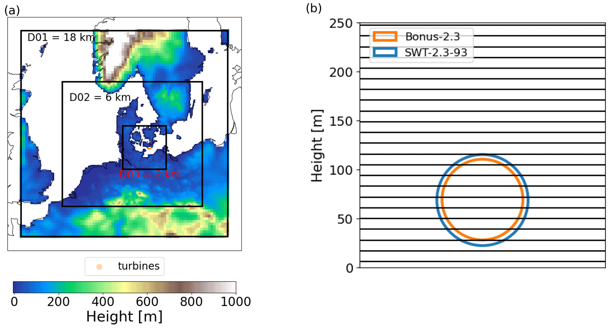
Figure 7 (a) Nested WRF domains with the innermost domain capturing the study area of the Fehmarn Belt with the Nysted and Rødsand II wind farms and (b) a vertical WRF grid with the lowest 14 mass levels and rotor areas covered by the two wind turbine models.

2.2.2 Engineering wake models

Three different rapid engineering wake models out of the open source wind farm simulation tool PyWake v2.2.0 (Pedersen et al., 2019) are applied in this study. The three wake deficit models, NOJ (Jensen, 1983), BAS (Bastankhah and Porté-Agel, 2014) and ZON (Zong and Porté-Agel, 2020), differ in complexity: the NOJ model has been developed for the far wake and represents the wake as a simple top-hat wake. We apply a linear wake expansion constant of k=0.04, which corresponds to offshore conditions and has been used in previous studies (Nygaard and Hansen, 2016). In contrast, BAS assumes a Gaussian distribution for the velocity deficit in the wake and has been derived assuming conservation of mass and momentum. It is valid only for the far wake, i.e. the region starting approximately 2–4 rotor diameters downstream of the turbine when the rotor geometry does not play a dominant role anymore, and has been validated against wind-tunnel measurements and large-eddy simulations with a linear wake expansion constant of k=0.03. The last model, ZON, simulates the wake expansion as a function of local TI (with parameters as described in Zong and Porté-Agel, 2020) and the approach of Shapiro et al. (2018) is used for the wake width expansion. All three wake models are combined with the same blockage deficit model, namely the updated self-similar deficit (SSD) model originally developed by Troldborg and Meyer Forsting (2017). In the update two changes have been made, which are documented in Pedersen et al. (2019): first, a linear fit is used radially to avoid large lateral induction tails; and second, the axial induction depends now on the C_T and axial coordinate. To account for the up- and downstream effect of each turbine, an iterative approach is chosen to represent the deficit caused by all wind turbines on all wind turbines (“All2Alliterative”). Individual deficits are superimposed using a squared sum for NOJ and BAS or using a linear sum for ZON. More details on the methods are available online at https://topfarm.pages.windenergy.dtu.dk/PyWake/ (Pedersen et al., 2019).

The simulations extend over the inner domain of the PyWakeEllipSys simulations (Fig. 4 dashed magenta area) but use 750 equally spaced grid points in the east–west direction and 375 equally spaced grid points in the north–south direction. This corresponds to a resolution of 59 m in the east–west direction and 84 m in the north–south direction.

2.2.3 Mesoscale wake modelling using WRF

Mesoscale model simulations for different wind farm scenarios have been conducted with WRF v4.2.2 with the settings in Table 4. The WRF simulations are performed using three nested domains with 18, 6 and 2 km horizontal resolution, respectively (Fig. 7). In the vertical direction a non-equidistant grid is used with a resolution of about 10 m within the rotor area following the recommendations by Siedersleben et al. (2020), Lee and Lundquist (2017) and Tomaszewski and Lundquist (2020), and in total there are 14 levels below 250 m (Fig. 7b).

Thompson et al. (2008)

Table 4 WRF parameterization, boundary conditions and forcing data employed for the performed simulations. The wind farm parameterizations EWP and FIT were only applied for some scenarios (see Table 7).

Wind farms effects are parameterized using both FIT (Fitch et al., 2012) and EWP (Volker et al., 2015). FIT and EWP differ mainly in two aspects: first, EWP accounts for a sub-grid scale vertical wake expansion based on the concept from Tennekes and Lumley (1972) as described in Volker et al. (2015), while FIT does not include sub-grid scale effects. Second, only FIT considers wind farms as an explicit source of turbulent kinetic energy (TKE), while EWP assumes that TKE develops solely through shear production in the wind farm wake. More details on their comparison can be found in Fischereit et al. (2022). FIT is applied here including the bug fix provided by Archer et al. (2020) with the recommended TKE coefficient of 0.25. Both parameterizations require turbine positions, the turbine model as well as thrust and power curves as inputs. Details on the turbine models are given in Table 1. The power and thrust curve of the two turbine models are shown in Fig. 3.

2.3 Simulated scenarios

For WRF a 1-month period, October 2013, is simulated. This period has been selected based on high availability of mast measurements and Rødsand II SCADA data (Sect. 2.1). The simulations are conducted as consecutive 5.5 d periods with an overlap of 12 h that is disregarded as spin-up. This method, which is similar to the method applied for the New European Wind Atlas (Dörenkämper et al., 2020), has the advantage that model drifts are avoided due to the frequent new initialization, but at the same time unnecessary computations during spin-up are kept to a minimum. Each 5.5 d period took roughly 6 h of simulation time on 64 CPUs.

In contrast to WRF, for PyWake and PyWakeEllipSys the simulations do not represent the conditions in October 2013. Instead a farm-to-farm flow case for eastern wind directions is simulated to be able to study the wind farm wake effect of Nysted on Rødsand II and compare the results against the SCADA data available only for Rødsand II (Sect. 2.1). To compare these flow case simulations with the real WRF simulations and real SCADA data, the WRF results and SCADA data are filtered for the same conditions as the simulated flow case. The details of the filtering are described in Sect. 2.3.2.

2.3.1 Selected flow case

The impact of wakes on power is largest just below rated wind speed (Lundquist et al., 2019). Thus, a wind speed range around 10 m s⁻¹ has been selected for this study, which is just below rated power for the SWT2.3-93 turbine of Rødsand II (Fig. 3).

Table 5 Simulated flow cases with the high-resolution wake models in terms of wind speed (WS), wind direction (WD) and inflow turbulence intensity (TI) at 69 m height. For scenario and wake model description see Sects. 2.2.1 and 2.2.2. ^* RANS–ABL simulations are only approximately neutral (for details see Sect. 2.2.1). Linear is abbreviated “lin”.

To realize these conditions in PyWakeEllipSys, 10 different wind directions between 62.5 and 112.5^∘ with a 5^∘ interval and four different wind speeds between 9 and 12 m s⁻¹ as shown in Table 5 are simulated for both inflow models (RANS–ABL and RANS–ASL; Sect. 2.2.1). As a post-processing step, the flow variables are Gaussian averaged (Gaumond et al., 2014) over the wind directions with a standard deviation of 5^∘ and the resulting four wind directions (82.5, 87.5, 92.5 and 97.5^∘) are subsequently linearly averaged over the different wind directions. Finally, the simulations are averaged over the four wind speeds weighted according to the simulated inflow wind speed from the filtered WRF–NWF simulation (Sect. 2.3.2). The chosen value of the standard deviation for the Gaussian averaging is based on the work of Gaumond et al. (2014), where a smaller standard deviation (2.7^∘) was estimated from net mast measurements, but a larger standard deviation (4.5–7.4^∘) was necessary in order to fit the modelled power of the individual wind turbine rows of the Horns Rev I wind farm with the measured power that includes wind direction uncertainty. The latter is further explained in van der Laan et al. (2015a) (also see Sect. 3.1.3), where it is shown that the standard deviation increases linearly with the distance from the location at which the inflow wind direction has been measured. Overall, the applied 5^∘ standard deviation in the present work is a rough estimate based on these previous works.

The setup of the simulated flow cases for PyWake is similar to the setup of PyWakeEllipSys. For PyWake 360 simulations with a 1^∘ interval and four different wind speeds between 9 and 12 m s⁻¹ as shown in Table 5 are performed. As for PyWakeEllipSys, a Gaussian filter for wind direction is applied to the PyWake results with a standard deviation of 5^∘. Afterwards the results are linearly averaged over the wind directions between 82 and 98^∘. The results are finally averaged over the four wind speeds weighted according to the simulated inflow wind speed from the filtered WRF–NWF simulation (Sect. 2.3.2).

To derive both the intra- and farm-to-farm effect, two different wind farm configurations are simulated with PyWake and PyWakeEllipSys (Table 5). In the first configuration, named NYRØ, the actual situation is simulated with both Nysted and Rødsand II present. In the second configuration, named RØ, only the Rødsand II wind farm is included. Using RØ in combination with NYRØ allows isolation of the effect of Nysted on Rødsand II for the different models. Depending on the chosen wake model and wind farm configuration, each PyWake simulation, i.e. for all wind speed and directions, takes about 1–2 h to complete on 32 CPUs. The PyWakeEllipSys simulations took about 1–2 h using 985 CPUs for each wind direction, wind speed, inflow model and wind farm case. The relatively high computational cost is caused by the strict convergence requirement in order to resolve wind farm induction and the large number of cells (258 million) that is partly used to capture the wind farm wakes.

2.3.2 Filtering methods

To make the 1-month WRF simulations comparable to the flow case simulated by PyWake and PyWakeEllipSys, WRF results for October 2013 have to be filtered for neutral conditions, eastern wind direction and wind speeds around 10 m s⁻¹.

Neutral conditions are detected using the Obukhov length as described in Sect. 2.1. For filtering to the wind speed range of interest (9–12 m s⁻¹), the wind speed measurements at the Rødsand II mast cannot be used, since they are affected by the wake of Rødsand II and Nysted and thus do not represent free stream velocities. Instead, the wind speed filtering is based on the WRF simulation without wind farms (NWF; Table 7) for which an upstream grid point from Nysted (Fig. 2) is used to detect the inflow conditions. Due to infrequent joint occurrence of easterly wind with flow in the wind speed range of interest during October 2013 (Fig. 8a), only very few 10 min samples could be identified. For filtering the wind direction, two different approaches, named f1 and f2, respectively, have been tested (Table 6). In f1 the wind direction filter is based on the WRF–NWF simulation at the WRF inflow grid point (Fig. 2). In f2 the filtering is based on observed wind direction at the Rødsand II mast, which represents more closely the conditions represented by the SCADA data of Rødsand II (Sect. 2.1). Two different methods are applied, since the WRF–NWF simulations indicated a wind direction change from the inflow to Nysted to the outflow of Rødsand II (Fig. 8b).

Table 6 Details on filter methods 1 and 2 and corresponding available number of 10 min periods, average inflow wind direction (WD) and average inflow wind speed (WS). The subscript “in” refers to the WRF inflow grid point, which is depicted along with the other locations in Fig. 2.

(Volker et al., 2015)(Fitch et al., 2012; Archer et al., 2020)(Volker et al., 2015)(Fitch et al., 2012; Archer et al., 2020)

Table 7 Periods and scenarios covered by the WRF simulations.

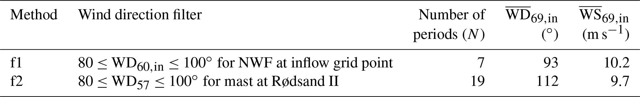
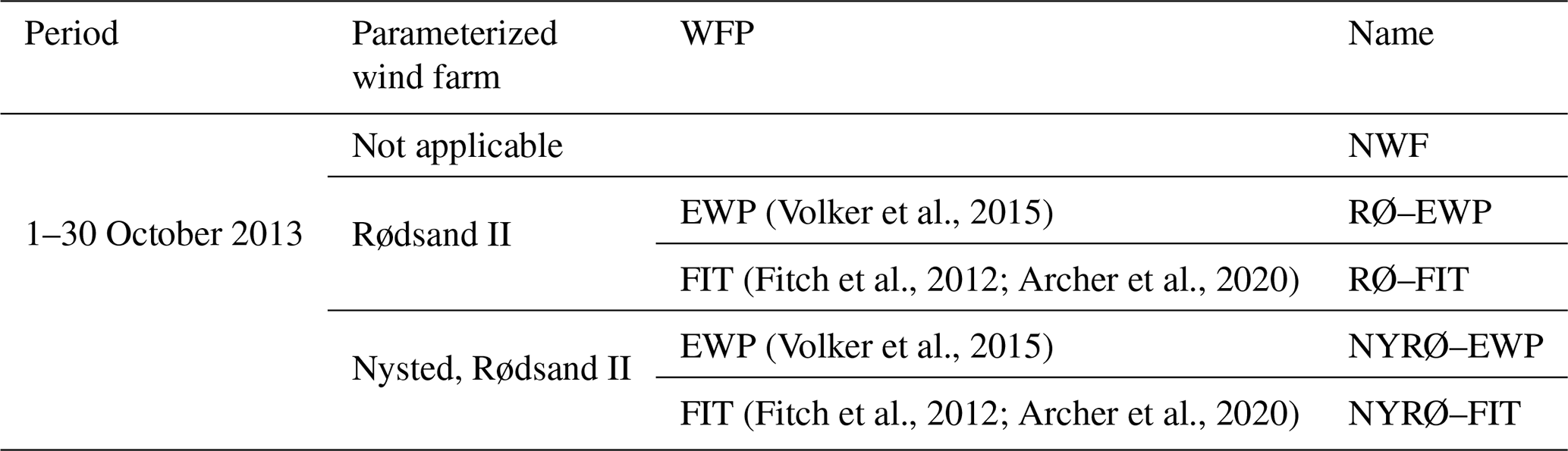
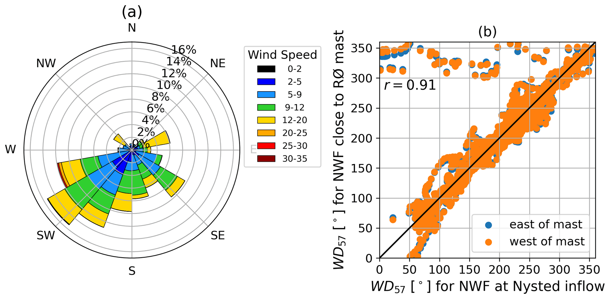
Figure 8 (a) Wake affected measured wind rose at the Rødsand II mast at 57 m height for October 2013 and (b) for NWF inflow wind direction at Nysted inflow grid point versus wind direction close to the mast. For locations see Fig. 2.

The described filtering for stability, wind speed and wind direction is applied to both SCADA data and the WRF results to identify N 10 min periods (Table 6), which are comparable to the simulated flow cases for PyWake and PyWakeEllipSys. Using the inflow wind speed for WRF–NWF for each 10 min period, the two closest simulated PyWake and PyWakeEllipSys inflow cases, i.e. rounded up (called WS_fl,u below) and rounded down (called WS_fl,l below), respectively, are identified and a weighted average ${\stackrel{\mathrm{‾}}{\mathrm{WS}}}_{\mathrm{fl},\mathrm{ave}}$ of the two corresponding simulations is calculated. The weight is calculated from $w=\mathrm{1}-({\mathrm{WS}}_{\mathrm{69},\mathrm{in},i}-{\mathrm{WS}}_{\mathrm{fl},\mathrm{l}})$, where WS${}_{\mathrm{69},\mathrm{in},i}$ is the WRF–NWF wind speed at the WRF inflow grid point (Fig. 2) for each period i. Using these weights, the average weighted flow case wind speed corresponding to the 10 min periods is then derived from

$$\begin{array}{}\text{(2)}& {\stackrel{\mathrm{‾}}{\mathrm{WS}}}_{\mathrm{fl},\mathrm{ave}}={\displaystyle \frac{\sum _{i=\mathrm{1}}^N\left({\mathrm{WS}}_{\mathrm{fl},\mathrm{l}}\cdot w+{\mathrm{WS}}_{\mathrm{fl},\mathrm{u}}\cdot (\mathrm{1}-w)\right)}{N}}.\end{array}$$

The WRF results and SCADA data for the identified 10 min periods are linearly averaged. The corresponding inflow wind speed for the two filter methods are listed in Table 6.

As for PyWake and PyWakeEllipSys, for WRF also NYRØ and RØ wind farm scenarios are simulated, which include Nysted and Rødsand II, and Rødsand II only, respectively. In addition, a third simulation, NWF, without any wind farm, is performed.

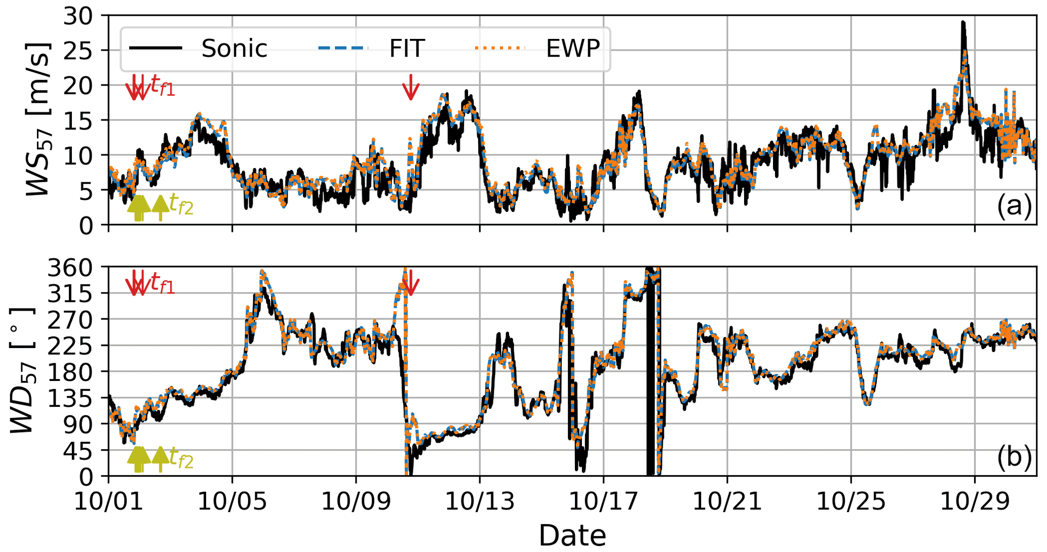
Figure 9 Time series of wind speed (WS, a) and wind direction (WD, b) at 57 m height for October 2013 for sonic mast measurements (black), and WRF results interpolated to the mast location for the NYRØ scenario for EWP (dotted orange) and FIT (dashed blue). The vertical arrows mark the time stamps t of the two filter methods f1 (red) and f2 (olive) according to Table 6. See Tables 6 and 7 for the abbreviations.

3 Results

The analysis of this study is split into two parts. First, the full 1-month WRF simulations are evaluated against mast measurements in Sect. 3.1. Second, the filtered WRF simulations and SCADA data are used to evaluate and compare the simulation results of the different wake models for intra-farm wakes (Sect. 3.2), farm-to-farm wakes (Sect. 3.3) and global blockage (Sect. 3.4).

3.1 Evaluation of WRF with mast measurements

The WRF simulations are compared against sonic measurements at the Rødsand II mast for October 2013 in Fig. 9 for both wind speed (WS) and wind direction (WD). In general, the time series for both WS and WD for FIT and EWP agree well with the sonic measurements with a few exceptions. The good visual agreement is confirmed by the high correlation coefficient of 0.88 for WS and 0.91 for WD (Fig. 10).

The simulation results gradually improve from NWF to NYRØ–EWP and NYRØ–FIT due to accounting for the wind farm effect (Fig. 10). The WS bias decreases from 1.06 m s⁻¹ for NWF to 0.73 m s⁻¹ for EWP and 0.52 m s⁻¹ for FIT (Fig. 10a–c). The WD bias reduces from 8.47^∘ for NWF to 7.86^∘ for EWP and 7.84^∘ for FIT. Thus, FIT clearly performs best for simulating WS at the mast, and the improvements for WD compared with NWF are similar for EWP and FIT. Looking at the black binned line in Fig. 10a–c, representing mean and standard deviations, it becomes clear that compared with NWF, both EWP and FIT show the largest improvements around 8–13 m s⁻¹, where the thrust is high (Fig. 3).

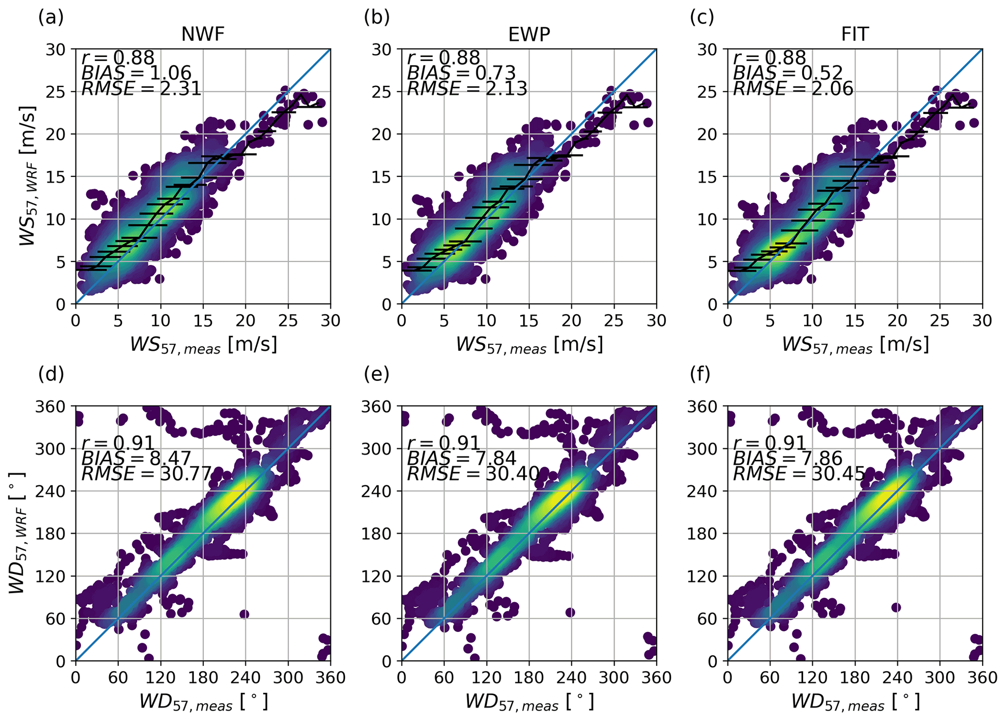
Figure 10 Scatter plot of measured (a–c) wind speed (WS) and (d–f) wind direction (WD) at 57 m height against WRF simulations, namely (a, d) NWF, (b, e) NYRØ–EWP and (c, f) NYRØ–FIT (Table 7) for October 2013.

The wind farm effect for the entire October 2013 at the mast can be derived by subtracting the WS bias of NWF from the WS bias of EWP or FIT, respectively. Doing so indicates a wind farm effect at 57 m height, i.e. 12 m below hub height, of 0.33 m s⁻¹ for EWP and 0.54 m s⁻¹ for FIT. These rather small wind farm effects can be explained by the location of the mast at the west of Rødsand II (Fig. 2), and the relatively frequent wind direction for October 2013 from the south-west (Fig. 8), when the mast is not much influenced by the wake of the farm, but only by global blockage. Performing the same analysis filtered for eastern wind directions ($\mathrm{90}\pm \mathrm{10}{}^{\circ }$) at the RØ mast, but without filtering for wind speed, indicates a considerably larger wind farm effect based on 127 10 min values: WS${}_{\mathrm{bias},\mathrm{NWF}}=\mathrm{1.04}$ m s⁻¹, WS${}_{\mathrm{bias},\mathrm{EWP}}=\mathrm{0.32}$ m s⁻¹ and WS${}_{\mathrm{bias},\mathrm{FIT}}=-\mathrm{0.14}$ m s⁻¹, which amounts to a wind farm effect of 0.73 m s⁻¹ for EWP and 1.2 m s⁻¹ for FIT at 57 m height that can be largely attributed to the wake effect of the farms. Selecting a non-wake-affected sector between 260 and 30^∘ for comparison shows that the bias is strongly reduced for the NWF scenario: WS${}_{\mathrm{bias},\mathrm{NWF}}=-\mathrm{0.02}$ m s⁻¹, WS${}_{\mathrm{bias},\mathrm{EWP}}=-\mathrm{0.17}$ m s⁻¹ and WS${}_{\mathrm{bias},\mathrm{FIT}}=-\mathrm{0.28}$ m s⁻¹, which would correspond to a wind farm effect of −0.15 m s⁻¹ for EWP and −0.25 m s⁻¹ for FIT. The larger biases for EWP and FIT compared with NWF for the non-wake-affected sector can be partly attributed to the interpolation of wake-affected and non-wake-affected points to the mast location.

3.2 Comparison of intra-farm wake modelling

3.2.1 Comparison of filter methods

To compare the flow cases modelled with PyWakeEllipSys and Pywake against the real WRF simulation and SCADA data for October, two different filter methods were proposed (Table 6). The two methods are compared in Fig. 11 for different south–north transects at different locations within the area of the wind farms in the east–west direction with (a) being the easternmost transect and (f) being the westernmost transect. Normalized relative coordinates are used by transforming the original coordinates x using

$$\begin{array}{}\text{(3)}& x_{\mathrm{rel},\mathrm{n}}={\displaystyle \frac{x-x_{\mathrm{ref},\mathrm{t}}}{D}},\end{array}$$

where x_ref,t is the location of the easternmost turbine of Rødsand II and D is the rotor diameter of the Rødsand II turbine model SWT-2.3-93 (Table 1). For readability, only the simulation results for WRF–NWF, WRF–FIT and RANS–ABL are shown; the simulation results for other simulations are shown in Figs. 12 and 13. Solid lines indicate results according to f1, whereas dashed lines refer to f2 (Table 6). Equivalent wind speed derived from SCADA data for the turbines close to the transect and filtered according to f1 and f2 are shown as cyan and green error bars, respectively, with mean (dots) and standard deviation over all periods (whiskers).

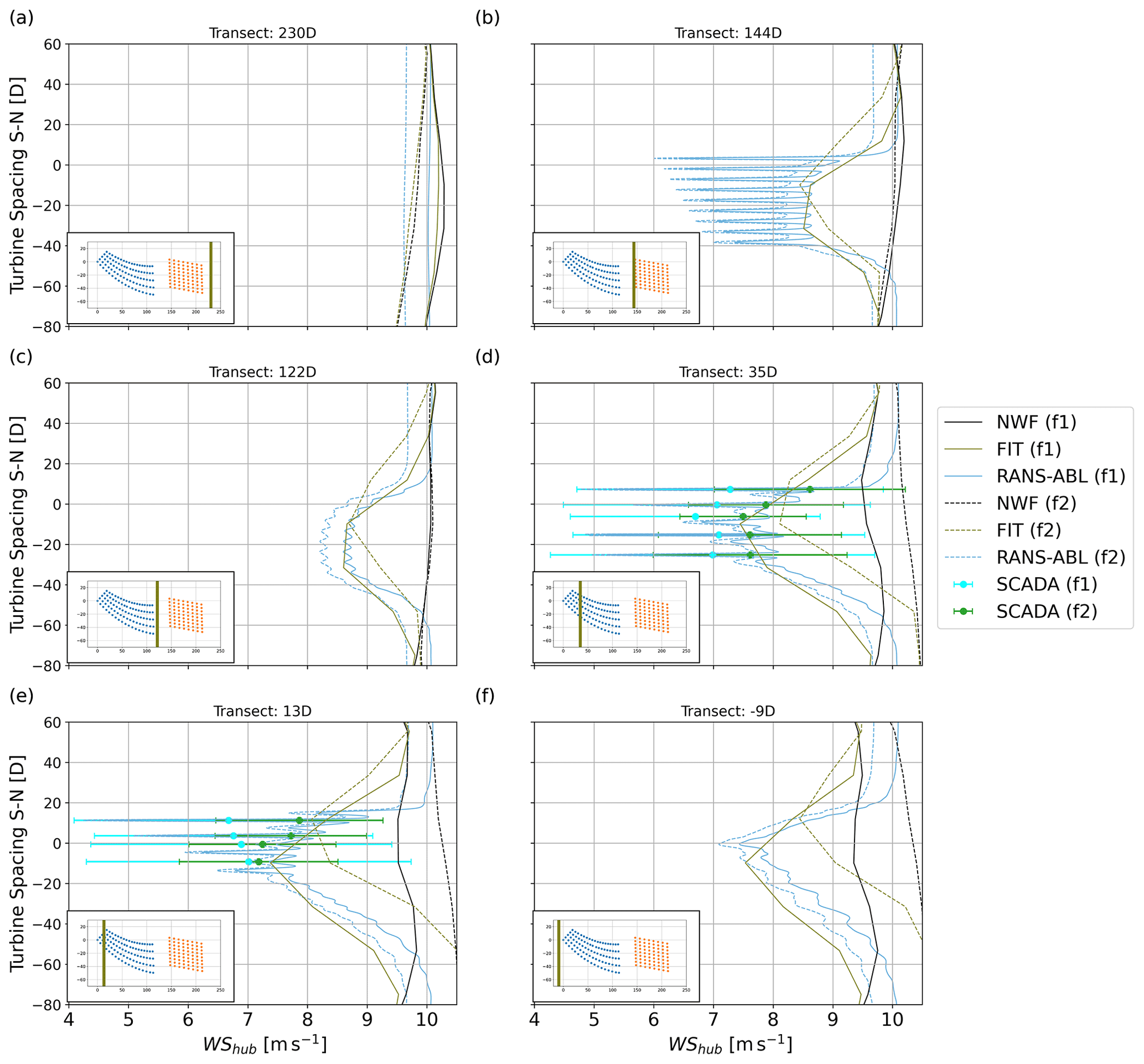
Figure 11 North–south transects for wind speed at hub height for different models at different locations in the east–west direction as indicated by the olive line in each subplot and the transect name in the title in normalized coordinates as explained in the text. All simulations are for NYRØ. For abbreviations see Tables 5 and 7, and see Table 6 for the f1 and f2 methods.

The WRF–NWF simulations show that while the two filtering methods agree well for the transects 144 and 122 D between Nysted and Rødsand II, they disagree for the inflow transect to Nysted (230D) and especially for the southern part of the transects in the area of Rødsand II (35, 13, −9 D). In accordance with the smaller average wind speed in f2 (Table 6), all f2 results are shifted towards smaller values. The simulations also reflect the average inflow directions for f1 and f2 (Table 6) in that the maximal wind speed deficits for f2 are shifted northwards compared with f1 and the RANS–ABL results.

While the inflow direction agrees better between models for f1, f2-filtered SCADA data agree better with RANS–ABL compared with f1: the average RMSE for f1 is 1.1 m s⁻¹, while it is 0.4 m s⁻¹ for f2. This is because for f2 the filtering uses the wind direction measurements at the Rødsand II mast, which is closer to Rødsand II than the inflow to Nysted for f1. The analysis of wind directions to the east and west of the two farms for WRF–NWF indicate wind direction changes over the domain (Fig. 8b). This could be related to coastal effects from the land area to the north of the farms but deserves further analysis. However, it indicates that even in this relatively small area of about 20 km, wind directions cannot simply be assumed to be unified across the area. This indicates that flow case simulations, like those performed with PyWake and PyWakeEllipSys in this study, need to be handled with care as the area of interest increases and when coastal effects could play a role.

The comparison of f1 and f2 indicates that both filtering methods have advantages and disadvantages: f1 represents better the inflow conditions of the simulated flow cases for PyWake and PyWakeEllipSys, while f2 compares better with the equivalent wind speed from SCADA. Thus, depending on the target analysis either method is used below.

3.2.2 Comparison of models

To facilitate the comparison between the real WRF simulations and the flow cases simulated with the other models as described in Sect. 2.3.1, the results are normalized with a no-wind-farm scenario. For WRF–FIT and WRF–EWP, WRF–NWF is used to do so. For the PyWake and PyWakeEllipSys simulations, the easternmost wind speed is used, which is not influenced by the presence of the wind farms. The normalized results are shown for the same transects as in Fig. 11 for the two filter methods in Figs. 12 and 13, respectively. The figures show the simulation results of all applied models abbreviated in accordance with Tables 5 and 7.

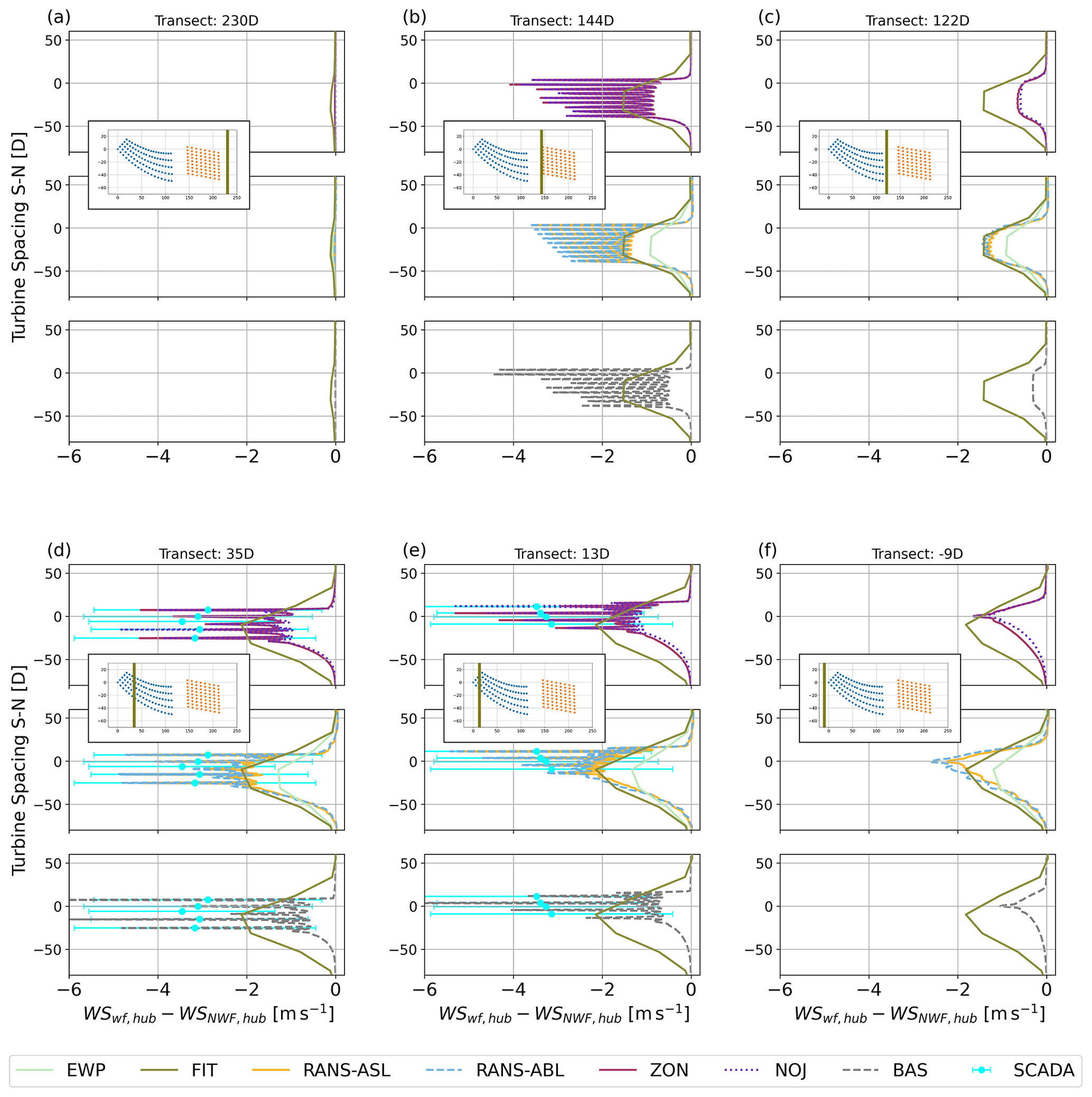
Figure 12 Wind speed transects at hub height for the different models in the north–south direction at different locations as indicated by the olive line in each subplot. The coordinates are relative to the coordinates of the easternmost turbine of Rødsand II and normalized with the rotor diameter of the Rødsand II turbine model SWT-2.3-93 (Table 1). All simulations are for NYRØ and normalized with a no-wind-farm (NWF) scenario. For abbreviations see Tables 5 and 7. WRF results and SCADA data are filtered according to the f1 method (Table 6). FIT and, if applicable, SCADA data are shown in each subplot to facilitate comparison of the different simulations.

Figure 13 The same as Fig. 12 but for filter method f2.

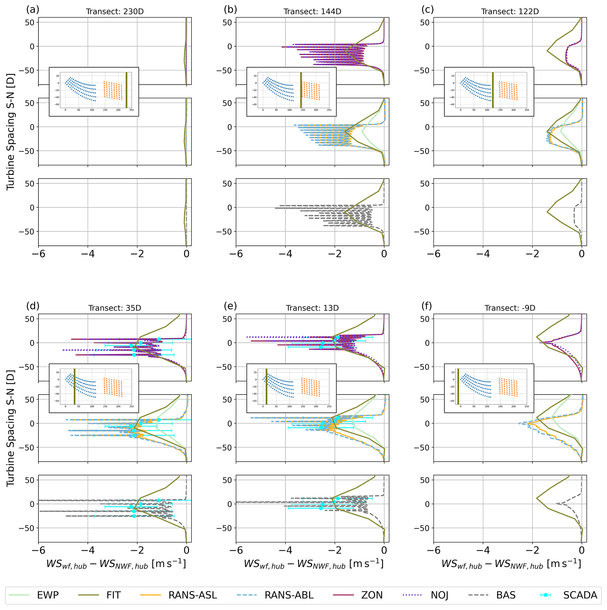
For both filter methods, the transect 230 D (Figs. 12a and 13a) show a global blockage effect of Nysted for the WRF and PyWakeEllipSys simulations. This will be discussed further in Sect. 3.4.

Transects 144, 35 and 13 D (Figs. 12b–e and 13b–e, respectively) are taken within or just outside the farms. As expected due to the coarse resolution, WRF–EWP and WRF–FIT cannot resolve the internal variability within the farms with large deficits of up to 5 m s⁻¹ very close to the individual turbines. However, especially WRF–FIT compares very well to the baseline deficit of RANS–ASL and RANS–ABL, i.e. the wind speed deficit in between the turbines, for all transects for f1 (Fig. 12). This is also true for f2 (Fig. 13), except that the maximum deficit is shifted northward in WRF due to the average wind direction being more southerly (Table 6) as discussed in Sect. 3.2.1. In contrast to FIT, EWP underestimates wind speed deficits when compared with both RANS–ASL and RANS–ABL. The equivalent wind speeds derived from SCADA data indicate that both RANS and WRF–FIT results are reasonable. This is true especially for f2 (Fig. 13), which better represents the actual situation close to Rødsand II as discussed in Sect. 3.2.1.

The results for the two RANS methods (Sect. 2.2.1) give pretty similar results. This is because the RANS–ABL model is employed with a relatively large ABL height resembling near-neutral conditions and the resulting inflow can be approximated by an atmospheric surface layer, as used by the RANS–ASL model.

The peak deficits of all applied wake models in PyWake, ZON, NOJ and BAS agree relatively well with the peak deficits for PyWakeEllipSys (transects 144, 35 and 13 D). However, the baseline deficits in PyWake are smaller compared with RANS and for ZON and NOJ comparable to those of WRF–EWP. In addition, the deficits are narrower in the south–north direction around the borders of the farm compared with the RANS results, especially for the transects downwind for Nysted (Fig. 12c–f). Downstream of the farms, the flow recovery for PyWake is very rapid, especially for BAS. Thus, the inflow to Rødsand II is not much reduced for BAS compared with the free-stream inflow to Nysted. This indicates that the chosen wake models in PyWake can represent the peak wind speed deficits within one wind farm well, but underestimate the effect of farm-to-farm wakes with different magnitudes as will be discussed in more detail in Sect. 3.3.

3.3 Comparison of farm-to-farm wake modelling

To isolate the effect of Nysted on Rødsand II, the difference between NYRØ and RØ, i.e. a simulation without Nysted, is investigated. Here only the results for f1 are presented, since the inflow conditions for those simulations agree better with the inflow conditions of the PyWake and PyWakeEllipSys simulations than the results for f2.

Figure 14 shows spatially the relative wind speed difference at hub height between NYRØ and RØ for the different models. As expected from the intra-farm analysis in Sect. 3.2.2, WRF–FIT results agree very well with the high-fidelity RANS results (Fig. 14b–d). WRF–EWP underestimates the wind speed reduction due to the presence of Nysted compared with RANS. While PyWake results (Fig. 14e–g) show strong deficits behind individual turbines, the wakes are very narrow and the influence on Rødsand II is much smaller compared with the results of the other models, as already expected from the analysis in Sect. 3.2.2. Out of the three investigated deficit models in PyWake, ZON shows the strongest farm-to-farm effect, which is, however, still smaller than the influence based on RANS and WRF.

Figure 14 Relative difference in hub height wind speed (WS) between NYRØ and RØ different wake models for filter method f1. For abbreviations see Tables 5 and 7.

The impact of Nysted on the flow extends beyond Rødsand II for EWP, FIT, RANS–ASL and RANS–ABL as indicated by reduced wind speeds west of Rødsand II. Comparing RANS–ASL and RANS–ABL, RANS–ABL shows slightly longer and stronger wakes. This is expected, since simulated inflow profile corresponds to slightly stable conditions, where wakes are generally longer (Cañadillas et al., 2020).

To quantify the impact of Nysted on Rødsand II, the wind speed and power reduction in the area of Rødsand II is shown in histograms in Fig. 15. In all subplots the difference between NYRØ and RØ are shown for f1 for different deficit classes as simulated over the brown area A1 in Fig. 2. Figure 15a and c show absolute differences for wind speed and power, respectively, between NYRØ and RØ and, Fig. 15b and d show normalized difference with the results for RØ. Power has been derived from the power curve for an SWT2.3-93 turbine (Fig. 3), the turbine type used for Rødsand II.

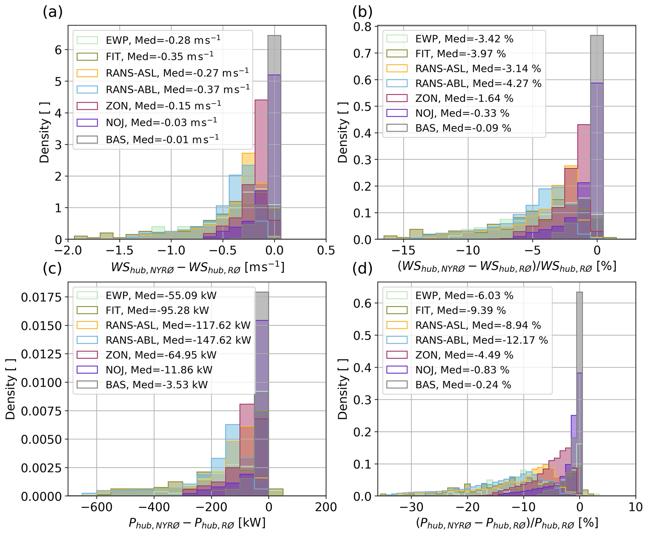
Figure 15 Histogram of reduction in (a, b) wind speed (WS) and (c, d) power (P) at hub height in the area of Rødsand II (solid rectangle around Rødsand II in Fig. 2) due to the presence of Nysted in terms of (a, c) absolute differences and (b, d) relative differences.

Median reductions in available wind speed resource for Rødsand II due to the presence of Nysted for the flow case of easterly wind around 10 m s⁻¹ are about 0.3 m s⁻¹ or between 50 and 150 kW for EWP, FIT and RANS. This corresponds to a relative reduction in available wind resources of 3 %–4 % or equivalently to 6 %–12 % reduction in power output compared with a scenario with a stand-alone Rødsand II wind farm without Nysted wind farm being present.

As expected from the previous analysis according to the PyWake simulations, the influence of Nysted on Rødsand II is much smaller for a flow case of around 10 m s⁻¹ (median around 0.3 % reduction in wind resources or up to 0.8 % reduction in power output). ZON, being the most complex engineering wake model used in this study, shows the largest reductions out of the three chosen wake models. Since the high-fidelity RANS and WRF simulations agreed better with SCADA data in Sect. 3.2.2, one can conclude that the chosen PyWake models in the current setup are not suited to study farm-to-farm wakes.

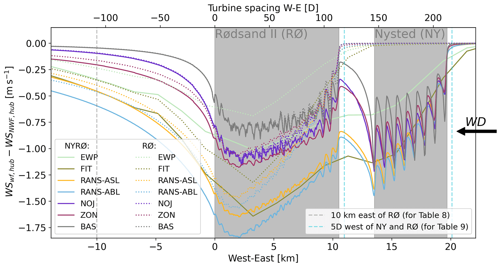
Figure 16 West–east cross section of wind speed deficit with respect to a no-wind-farm (NWF) scenario averaged in the north–south direction over the pink area A2 in Fig. 2 for the f1 filter method. NWF corresponds to RANS and PyWake for the easternmost grid points and to EWP and FIT for the NWF simulation. The arrow indicates the wind direction (WD). Solid lines correspond to the scenario NYRØ, while dotted lines correspond to the scenario RØ. For abbreviations see Tables 5 and 7.

Comparing the WRF simulations with the PyWakeEllipSys simulations in more detail indicates that the median wind speed reductions due to the presence of Nysted for EWP and FIT lie in between those for RANS–ASL and RANS–ABL. Thus, concerning estimating median farm-to-farm wake effects, both EWP and FIT provide reasonable results. Since power is more sensitive to wind speed deviations due to the cubed relationship between wind speed and power, for power FIT performs better than EWP when compared with the two RANS simulations.

WRF and RANS reduction distributions have a long tail ranging up to 15 % reduction in available wind resources or equivalently up to 35 % reduction in power output due to the presence of Nysted. In terms of looking at the full distributions, FIT visually agrees better with RANS–ABL than EWP. The RANS–ASL results are shifted to smaller reductions compared with RANS–ABL, which is expected due to the pure neutral stratification used in RANS–ASL compared with RANS–ABL, where near-neutral conditions are employed.

To better understand the wake recovery of the different wake models, west–east cross sections with averaged wind speed deficit in the north–south direction over the dashed area in Fig. 2 are shown in Fig. 16 for both NYRØ (solid lines) and RØ (dotted lines) for the different wake models (colours). Wind speed deficits at hub height with respect to a no-wind-farm (NWF) scenario are shown. As before, the NWF scenario for RANS and PyWake corresponds to the easternmost grid points, which are undisturbed by the presence of the farms, and for EWP and FIT to the WRF–NWF simulation.

The cross section highlights again the strong intra-farm variability in RANS–ASL, RANS–ABL, NOJ, ZON and BAS that cannot be captured with FIT and EWP due to the coarser resolution. It shows also that the ZON and NOJ results compare better with the RANS results for Nysted than BAS, since they can capture an accumulated wind speed deficit from east to west in Nysted. However, compared with RANS, all PyWake models recover fast and show a much smaller reduction in the Rødsand II area.

Comparing the RANS results with EWP and FIT shows again the better agreement between RANS and FIT for both farms. Overall FIT results lie in between RANS–ABL and RANS–ASL for NYRØ (solid lines) and are therefore considered to well suited to study farm-to-farm effects. EWP shows smaller deficits than RANS in Rødsand II and the results lie in between ZON and BAS. Thus, EWP agrees more with the engineering wake models than with RANS–CFD.

Comparing the results for NYRØ (solid lines) and RØ (dotted lines) indicates again that the effect of Nysted on Rødsand II is minimal for BAS (barely visible at the eastern part of Rødsand II) and increases over NOJ to ZON. In contrast, substantial differences in available wind resources of about between 1 m s⁻¹ at the inflow to Rødsand II and about 0.25 m s⁻¹ towards the outflow of Rødsand II exist for RANS and WRF. Thus, in addition to a distribution of resource reductions due to the presence of Nysted (Fig. 15), the reductions differ spatially with larger reductions close to Nysted. This is expected, since Nysted's influence is strongest close to the farm itself. However, even far west of Rødsand II, the NYRØ and RØ scenarios differ in wind speed, meaning the effect of Nysted on the flow still can be seen at the western edge of the figure, i.e. 27.5 km downstream of Nysted.

Table 8 Wind speed deficit at the closed grid point (for PyWake and PyWakeEllipSys) and interpolated (for WRF) for each model to 10 km east of Rødsand II (dashed grey line in Fig. 16) for the different wake models. All results are averaged in the north–south direction over the pink area A2 in Fig. 2.

Table 9 Wind speed deficit 5 rotor diameter ahead of Nysted (for NYRØ) and 5 rotor diameter ahead of Rødsand II (for RØ) for the different wake models. Results are taken from the closed grid points for PyWake and PyWakeEllipSys and are interpolated to 5 rotor diameter for WRF. All results are averaged in the north–south direction over the dashed pink area A2 in Fig. 2.

To quantify this difference in long-distance wakes, wind speed deficits with respect to a no-wind-farm scenario are quantified for NYRØ and RØ 10 km downstream of Rødsand II in Table 8. This distance has been chosen since it is still relatively undisturbed from the island of Fehmarn, which affects the WRF results further downstream (dashed area in Fig. 2) and is not considered in the PyWake and PyWakeEllipSys simulations. For WRF, a weighted average based on the distance of the closest two grid points is used, while for PyWake and PyWakeEllipSys the closest grid point is chosen, which is close enough due to the high resolution of those simulations.

Comparing the wind speed deficit 10 km downwind of Rødsand II (Table 8) indicates that BAS shows almost no wind speed deficit (0.05 m s⁻¹ or about 0.5 %). NOJ still shows deficits about 0.1 m s⁻¹ or about 1 %, while ZON, EWP, FIT and RANS still show deficits of 0.2–0.6 m s⁻¹ (2 %–6 %). Comparing the difference between NYRØ and RØ at the same location based on two significant digits, no difference for NOJ and BAS is visible underlining the rapid wake recovery of these two models. ZON still shows a difference due to the presence of Nysted of 0.5 % 10 km downstream, i.e. half of the difference for RANS and WRF (0.1 m s⁻¹ or 1 %).

This shows that wind resources are affected by wind farms more than 25 km away according to the RANS and WRF simulations. Thus, farm-to-farm wakes are important to consider for more than 25 km for wind speed ranges just below rated wind speed even for neutral conditions. This agrees relatively well with the flight measurements presented in Cañadillas et al. (2020), although with some uncertainty, since they only show snapshots for three neutral and unstable cases.

3.4 Comparison of global blockage effect modelling

The main focus of this study is the comparison of wake modelling for different classes of models. However, it also gives the opportunity to look at the modelling of global blockage effect ahead of Rødsand II and Nysted. To do so, the wind speed deficit with respect to a no-wind-farm scenario is investigated at a distance of before 5 rotor diameters upstream of each farm. Due to the different turbine types of the two farms (Table 1), this is 412 m upstream for Nysted and 465 m for Rødsand II and is shown as dashed light blue lines in Fig. 16. As for the analysis of the long-distance wake effect, WRF results are calculated from an average of the closest grid points weighted by distance to the point of interest, while for PyWake and PyWakeEllipSys the closest grid points in the east–west direction are used. To investigate the global blockage effect of Nysted the NYRØ scenario is used, whereas for Rødsand II the RØ scenario is used, since in NYRØ also the wake effect of Nysted is present. The results for the different models are summarized in Table 9.

The global blockage model selected for PyWake, SSD (Sect. 2.2.2), shows the smallest blockage effect (<1 %), followed by the RANS simulations (between 0.3 % and 0.4 %) and WRF simulations (between 0.9 % and 2.3 %). Consistent across all models, the blockage effect is smaller for Rødsand II than for Nysted. This could be due to the different shape or being an artefact of the chosen average area. Based on the very few existing blockage measurements, negligible blockage is expected for neutral and unstable conditions as shown in Schneemann et al. (2021) from scanning lidar measurements. In stable conditions the global blockage effect can amount to 2 %–6 % (Schneemann et al., 2021). The global blockage effect for WRF is likely overestimated, since a wake-affected grid point and a non-wake-affected grid point are averaged here to extract the results at a location similar to that for PyWake and PyWakeEllipSys. Due to the coarse resolution of WRF, which assumes the same wind speed for the entire 2 by 2 km area, this result is very much grid dependent and could change for a slightly different WRF grid. Thus, these results should be treated qualitatively and not quantitatively.

4 Discussion and conclusion

Simulations for the two neighbouring wind farms, Nysted and Rødsand II, in the Fehmarn Belt area are performed with models of different complexity, fidelity, scale and computational costs. The results are compared for the simulation of intra-farm and farm-to-farm wakes as well as for the simulation of wake recovery and global blockage effect both against each other and against SCADA data. The model complexity ranges from mesoscale model simulations with two different wind farm parameterizations (WRF–EWP and WRF–FIT), over high-resolution CFD–RANS model simulations equipped with an actuator disk model using PyWakeEllipSys employing two different inflow models (RANS–ASL and RANS–ABL) and three rapid engineering wake models included in the PyWake suite (NOJ, ZON and BAS).

The analysis of the real WRF simulations for a 1-month period in October 2013 indicated that the WRF model can well represent the meteorological conditions for that period. Compared with wind farm wake influenced mast measurements of wind speed, FIT (WS bias: 0.52 m s⁻¹) performs better than EWP (WS bias: 0.73 m s⁻¹); however, EWP still improves the evaluation compared to a simulation without wind farms.

Comparing the filtered WRF results to a farm-to-farm flow case that has been simulated with PyWake and PyWakeEllipSys shows that, as expected from the coarse mesoscale resolution, FIT and EWP cannot capture peak wind speed deficits downstream of individual turbines. However, especially FIT compares well with the baseline wind speed deficit simulated by PyWakeEllipSys. EWP underestimates the wind speed deficits compared with the RANS simulations. However, both EWP and FIT can well estimate median wind resource reductions due to the presence of an upstream farm. Expected median reductions in power output are better represented in FIT than in EWP when compared with RANS.

The engineering wake models in the PyWake suite agree reasonably well with the RANS simulations within Nysted and at its outflow. However, all engineering models simulate a much more rapid wind deficit recovery downstream of the wind farms and thus a one order of magnitude smaller farm-to-farm wake effect. Considering the agreement of WRF and PyWakeEllipSys and their agreement with the SCADA data, all considered engineering wake models likely underestimate the wind farm wake effect. Thus, the results of these wake models should not be trusted when farm-to-farm wakes are an issue, although they can well represent intra-farm wakes. However, using a more sophisticated deficit model, like ZON, can improve the prediction of a farm-to-farm effect compared with simpler models. However, all rapid engineering wake models are only as good as their calibration data sets. Future work could consider farm-to-farm calibration data sets in addition to intra-farm calibration data sets to improve their capability.

The analysis of the long-distance wakes showed that even in neutral conditions, the effect of an upstream farm can still amount to a wind resource reduction of 1 % 25 km downstream. This is consistent for both RANS and WRF simulations and indicates that farm-to-farm effects should not be neglected for wind resource planning offshore.

The study also shows challenges when comparing idealized flow cases with real data: the NWF simulations indicated that wind direction over the study area is likely influenced by coastal effects. This leads to spatial variability in the flow, especially with respect to wind direction over this 40 km area of interest. More measurements are required to verify this wind direction variability across the domain of the two wind farms. However, this still indicates that for offshore farms close to the coast, uniform inflow flow cases cannot capture the variability due to local effects downstream. Thus, for more accurate high-resolution wind simulations, these effects should be accounted for when applying high-resolution models in the future.

The flow case selected for this study represents a situation with strong influence of wakes, since a wind speed range just below rated wind speed has been chosen. The results could be extended by considering other wind speed ranges to generate a more complete picture. The selection of the simulation period was constrained by the available measurements. However, due to the infrequent occurrence of easterly flow, only very few relevant time stamps could be identified. Thus, the results contain some uncertainty. Other periods as well as the evaluation of wind farm pairs with other layouts should be investigated in further studies to confirm the results from this study.

In this study, we applied a TKE factor of 0.25 in the FIT parameterization (Table 4) following the recommendations of Archer et al. (2020). Based on our simulations, this seems to be a reasonable choice as the FIT simulations agree well with the RANS simulations. However, since we only tested this coefficient and focused only on the evaluation of wind speed deficit, we cannot conclude that 0.25 is the best choice in all conditions. Larsén and Fischereit (2021), for instance, compared WRF–FIT simulations against flight measurements and found that for their simulation a TKE factor of 1 was more appropriate. Thus, more studies are needed to derive the best TKE factor.

A resolution of 2 km was applied in this study, which is a typical resolution of mesoscale models for wind energy applications according to the review by Fischereit et al. (2022). We showed that baseline intra-farm wakes can be captured reasonably well with this resolution. A higher resolution of, for example, 1 km could be tested to see whether the agreement improves even more.

Considering the two main aims of this study, we can conclude that baseline intra-farm wind speed variability, i.e. the wind speed deficit in between turbines, can be captured reasonably well with the Fitch et al. (2012) wind farm parameterization using a resolution of 2 km, while EWP underestimates wind speed deficits. The considered RANS model, PyWakeEllipSys, can simulate wind farm wakes and long-distance wakes well, but even for relatively small areas offshore uniform inflow conditions are not always met near the coast. Thus, if long-distance wakes are of interest, effects of terrain and roughness should be considered in future PyWakeEllipSys simulations for coastal areas to provide a more realistic picture, following, for instance, the approach in van der Laan et al. (2017). However, mesoscale phenomena, like sea breezes, cannot be accounted for in CFD–RANS models, which is the strength of using mesoscale models like WRF. All considered engineering wake models from the PyWake suite underestimate the wind farm wake effect, although with different magnitudes. The most complex of the engineering deficit models applied here, ZON, provides the best option to account for a farm-to-farm effect among the tested rapid models. However, it still underestimates the median wind resource reduction, due to an upwind farm, by about 50 %. Therefore, overall, the higher computational costs of PyWakeEllipSys and WRF pay off in terms of accuracy for farm-to-farm wake modelling compared with rapid models like PyWake.