High-resolution offshore wind resource assessment at turbine hub height with Sentinel-1 synthetic aperture radar (SAR) data and machine learning

This paper presents a method for estimating offshore extractable wind power at hub height using Sentinel-1 synthetic aperture radar (SAR) data and machine learning. The method was tested in two areas off the Dutch coast, where measurements from Doppler wind lidars installed at the sea surface were available and could be used as a reference. A first machine learning algorithm improved the accuracy of SAR sea surface wind speeds by using geometrical characteristics of the sensor and metadata. This algorithm was trained with wind data measured by a large network of weather buoys at 4 m above sea level. After correction, the bias in SAR wind speed at 4 m versus buoys was 0.02 m s⁻¹, with a standard deviation of error of 0.74 m s⁻¹. Corrected surface wind speeds were then extrapolated to hub height with a second machine learning algorithm, which used meteorological parameters extracted from a high-resolution numerical model. This algorithm was trained with lidar vertical wind profiles and was able to extrapolate sea surface wind speeds at various altitudes up to 200 m. Once wind speeds at hub height were obtained, the Weibull parameters of their distribution were estimated, taking into account the satellites' irregular temporal sampling. Finally, we assumed the presence of a 10 MW turbine and obtained extractable wind power with a 1 km spatial resolution by multiplying the Weibull distribution point by point by its power curve. Accuracy for extractable wind power versus lidars was ± 3 %. Wind power maps at hub height were presented and compared with the outputs of the numerical model. The maps based on SAR data had a much higher level of detail, especially regarding coastal wind gradient. We concluded that SAR data combined with machine learning can improve the estimation of extractable wind power at hub height and provide useful insights to optimize siting and risk management. The algorithms presented in this study are independent and can also be used in a more general context to correct SAR surface winds, extrapolate surface winds to higher altitudes, and produce instantaneous SAR wind fields at hub height.

1 Introduction

Estimating extractable offshore wind power at turbine hub height is a challenge due to the difficulty of measuring the wind profile in the boundary layer over the sea. It is currently estimated using numerical models and/or Doppler wind lidars installed at the sea surface and pointing upwards (see, for example, Optis et al., 2021). Lidars provide the complete wind profile at a single location with a high temporal sampling but are very expensive to operate. Therefore, only one or two are typically used in site assessment. Conversely, numerical models provide outputs over the entire area of interest but are not capable of resolving small-scale phenomena due to their physics and resolution. As a result, any errors are not precisely known and may vary in time and space, which is particularly problematic in coastal areas where processes are more complex and on a smaller scale. Due to these limitations, considerable uncertainty remains regarding actual offshore wind resources, which can affect wind farm project planning and management.

The need to improve wind speed assessment and thus estimate more precisely wind power availability throughout the wind farm life cycle has led to growing interest in the use of satellite data (see, for example, Hasager et al., 2015). Unlike ground-based lidars, spaceborne sensors have the advantage of conducting sounding over large areas. However, they also have limitations: their revisit period is typically long (a couple of days for Sentinel-1 in Europe) and they use an indirect measurement based on sea state backscatter. Therefore, their measurements are impacted by several sources of potential error (low temporal sampling, sensor geometry, currents, algae, rain cells, bathymetry, turbulence, bright targets such as ships). Moreover, the extrapolation of their measurements from sea surface to hub height is not an easy task due to the variety of meteorological conditions that may impact the wind speed extrapolation ratio.

Several studies have attempted to assess offshore wind power potential using spaceborne scatterometers, including ERS-1, ERS-2, NSCAT, QuikSCAT, and ASCAT (Sánchez et al., 2007; Pimenta et al., 2008; Karagali et al., 2014; Bentamy and Croize-Fillon, 2014; Remmers et al., 2019). However, the resolution of these instruments is 12.5 km² at best, which is not adapted to coastal areas due to land contamination. Synthetic aperture radar (SAR) satellites are an interesting alternative because SAR wind products have a much finer resolution of 1 km. The potential of SAR data has already been assessed by numerous studies (Hasager et al., 2002, 2005, 2006, 2011, 2015, 2020; Christiansen et al., 2006; Chang et al., 2014, 2015). However, limited studies have been conducted validating SAR measurements using in situ data (Ahsbahs et al., 2017, 2020; Badger et al., 2019; de Montera et al., 2020), and these studies concluded that important biases remained (the term “in situ” includes profiling lidars, even though they use remote sensing). One reason for this is that SAR surface winds are obtained by inverting the backscatter with geophysical model functions (GMFs) originally designed for scatterometers, although differences from the SAR backscatter may occur due to different resolutions and the lack of inter-calibration between these two technologies. Another reason is that GMFs were designed empirically using the European Centre for Medium-Range Weather Forecasts (ECMWF) numerical model as a reference, which may not be accurate in coastal areas (in situ data were used only for validation and a posteriori bias correction; see Stoffelen et al., 2017, and references therein). In addition, GMFs may not fully capture the complex relation between sea state and wind speed, in particular because they assume a neutral atmosphere. Therefore, it is necessary to improve the accuracy of SAR wind speeds obtained with GMFs. This is particularly important given that wind power is related to the cube of wind speed and is therefore very sensitive to estimation errors.

Regarding the extrapolation of surface wind speeds to higher altitudes, the statistical theory of turbulence provides theoretical wind profiles (see, for example, Grachev and Fairall, 1996). However, this problem has not been satisfactorily solved and becomes increasingly critical as the typical height of wind turbines increases. Empirical evidence from offshore meteorological masts suggests that a simple power law could be sufficient to model the wind profile (Hsu et al., 1994). Nevertheless, above a few dozen metres, the power law model is questionable (see, for example, Tieo et al., 2020). This limitation has led some authors to use numerical model outputs to improve extrapolation to higher altitudes (Badger et al., 2016). The advantage of numerical models is that they provide information on atmospheric stability through parameters such as surface temperature and surface heat flux. In Badger et al. (2016), these surface parameters were averaged and combined with the similarity theory of Monin–Obukhov to extrapolate wind Weibull parameters. However, to our knowledge, this method was validated using only one meteorological mast in the Baltic Sea with an altitude not exceeding 100 m. Therefore, more research is needed to improve the extrapolation of SAR wind speeds to hub height and convince the industry to use them.

Machine learning seemed appropriate to us for improving SAR wind speed retrieval due to the variety of error sources. We used a large network of weather buoys to train the algorithm in order to cover a wide range of sensor angles. Regarding the extrapolation to higher altitudes, machine learning also seemed appropriate due to the complexity of the problem. Machine learning had already been found to improve the accuracy of extrapolated wind speeds, compared to power laws or logarithmic laws (Türkan et al., 2016; Mohandes and Rehman, 2018; Vassallo et al., 2020) and theoretical approaches (Optis et al., 2021). Moreover, Bodini and Optis (2020) showed that a machine learning algorithm trained in one location could be applied to a large surrounding area without significantly degrading its performance. Another advantage of machine learning compared to theoretical approaches is that it is not limited to the boundary layer and can be trained at any altitude. As in Badger et al. (2016), we took advantage of a numerical model to assess atmospheric stability and extract relevant meteorological parameters. These parameters were used as input for the machine learning algorithm, which was trained with lidar wind profiles measured in the North Sea.

Section 2 describes the SAR data, the high-resolution numerical model, and the in situ data used as a reference to train and validate the algorithms. Section 3 presents the algorithms and the method used to compute the extractable wind power. It also provides some insight into the effect of the sample number on method accuracy, plus a specific method for correcting SAR irregular temporal sampling. Section 4 presents the performance of the two machine learning algorithms and a test of the method in two areas off the Dutch coast. The resulting maps of the extractable wind resource are presented and compared with the outputs of the high-resolution numerical model in order to estimate the benefits of using this method compared with state-of-the-art techniques.

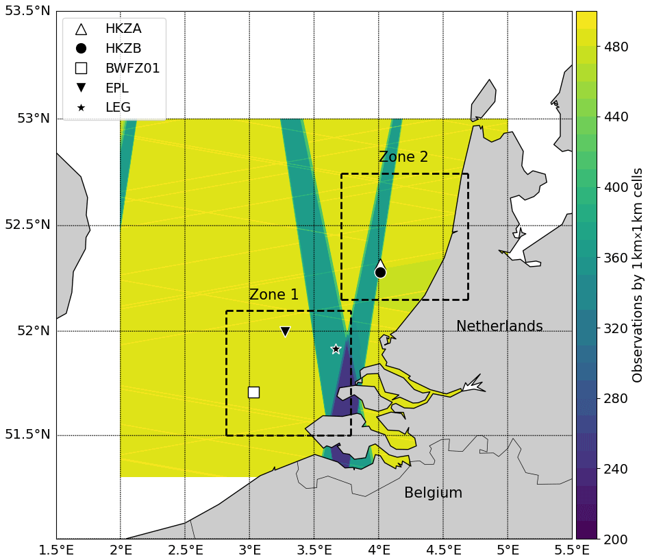
Figure 1 Locations of Zone 1 (bottom; 51.50–52.09^∘ N, 2.82–3.77^∘ E) and Zone 2 (top; 52.15–52.74^∘ N, 3.71–4.68^∘ E) with the positions of the profiling lidars. Colours represent the number of Sentinel-1 SAR Level-2 observations over a 2-year period (June 2016 to June 2018).

2 Data

2.1 Areas of study

The two areas of study are located off the Dutch coast (Fig. 1) and each measure approximately 70 km × 70 km. Their geographic extent was defined to include offshore profiling lidars and parts of the coastline in order to observe the wind speed coastal gradient.

2.2 Sentinel-1 SAR data

Sentinel-1A and Sentinel-1B are two polar-orbiting satellites equipped with C-band SAR. This sensor, which records surface roughness, has the advantage of operating day and night at wavelengths not impeded by cloud cover. The Sentinel-1 Level-1 Ground Range Detected (GRD) backscatter product has a spatial resolution of a few dozen metres, whereas Level-2 wind products typically have a spatial resolution of 1 km. The two satellites are located at the same orbit 180^∘ apart and at an altitude close to 700 km. In Dutch coastal waters, the acquisition mode is an interferometric wide swath using the TOPSAR technique, which provides a better-quality product by enhancing image homogeneity (De Zan and Guarnieri, 2006). The revisit rate is one passage every 2 d, which occurs around 05:00 or around 17:00 (UTC). The satellites pass in the morning or in the evening depending on the orbit orientation, descending or ascending, respectively. The exact acquisition time can vary by plus or minus 30 min, depending on the incidence angle under which the region of interest is observed. The number of samples over 2 years for the areas of interest is shown in Fig. 1, where it can be seen that coverage was not spatially uniform.

Level-1 images were calibrated and corrected from the instrument noise provided as metadata. Dedicated bright target filtering was applied to remove radar echoes created by ships, wind farms, and other structures at sea. An additional filter (Koch, 2004) was used to identify heterogeneous signatures not related to wind, such as currents, radar interferences, and remaining bright targets. However, since this filter has increased sensitivity at low wind speeds, the identified pixels were not removed to avoid disrupting the wind speed Weibull distribution, which is necessary to estimate wind power. The information provided by this filter was only used to create a quality flag, indicating areas where wind power estimates were unreliable, typically due to dense regions of wind turbines or mooring areas (see Sect. 4). Level-1 SAR products were then degraded to a 1 km resolution, and Level-2 surface winds at 10 $\mathrm{m}\mathrm{a}.\mathrm{s}.\mathrm{l}.$ were created using a Bayesian inversion scheme with two inputs: the wind vector obtained by inverting SAR backscatter with the CMOD7 GMF (Stoffelen et al., 2017) and the wind vector obtained from the ECMWF numerical weather prediction (NWP) model. Level-2 product tiles were finally combined into a gridded map over the areas of interest in order to form a data cube where each pixel corresponded to a time series of SAR wind speed measurements.

2.3 High-resolution numerical model

We used the Weather Research and Forecasting (WRF) non-hydrostatic meso-scale model (Skamarock et al., 2019) with a resolution of 1 km. The planetary boundary layer (PBL) parametrization of the model was based on Hahmann et al. (2020). WRF was forced at its boundaries by a downscaled larger-scale model, the reanalysed ERA5 (Hersbach et al., 2020) developed by ECMWF that has an hourly temporal resolution. WRF was run over the areas of study from December 2015 to June 2018 in order to cover the period during which lidar campaigns and Sentinel-1 data overlapped.

WRF provides wind speed and wind direction from sea level to 200 m in 20 m increments, as well as other variables such as air and sea surface temperature, surface heat flux, relative humidity, and pressure. These meteorological parameters were used to create the input parameters for the extrapolation algorithm. Moreover, since WRF is typical of numerical models currently used by industry, we also used it as a reference to assess the benefits of using SAR data. Since the industry often combines numerical models with in situ measurements, we also assessed the WRF outputs using available lidar data. WRF was found to underestimate extractable power by 3 % on average across all lidars. We corrected this bias before using WRF as a reference in the maps presented in Sect. 4.

2.4 NDBC buoy network

The buoy dataset consisted of 10 min averaged wind speeds from the National Data Buoy Center (NDBC) of the United States of America (USA). This network has the advantage of combining a large number of instruments, a large spatial coverage, and a standardized processing and quality check (Meindl and Hamilton, 1992). We selected only buoys measuring wind speed at 4 m so that the dataset was homogeneous in height and obtained with a similar type of instrument. A total of 12 buoys are located on the east coast of the USA (stations 41004, 41009, 41010, 41013, 41025, 41043, 44007, 44017, 44018, 44020, 44025, 44065), 18 on the west coast of the USA (stations 46011, 46012, 46014, 46015, 46022, 46025, 46026, 46027, 46028, 46041, 46042, 46047, 46050, 46053, 46054, 46069, 46084, 46086), 9 in the Gulf of Mexico (stations 42002, 42003, 42012, 42035, 42036, 42039, 42055, 42056, 42060), and 3 around the islands of Hawaii (stations 51000, 51002, 51003).

Table 1 Main characteristics of the five profiling lidars.

2.5 Lidar data

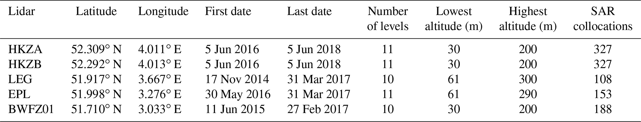
The dataset comprised five ground-based profiling lidars located off the Dutch coast (Fig. 1): HKZA, HKZB, BWFZ01, EPL, and LEG. HKZ stands for Hollandse Kust Zuid wind farm, BWF for Borssele Wind Farm Zone, EPL for European platform, and LEG for Lichteiland Goeree platform. Zone 1 included lidars BWFZ01, EPL, and LEG, and Zone 2 included lidars HKZA and HKZB. Lidars HKZA, HKZB, and BWFZ01 are floating, whereas lidars EPL and LEG are installed on platforms. These lidars provide 10 min averaged wind speed and wind direction. The data were quality checked by our data provider C2Wind (for each time interval, the minimum number of packets was set at 20 and the minimum availability at 80 %). The vertical sampling and duration of these lidar measurements varied between observation campaigns and are displayed in Table 1.

Many of the lidar altitude levels were similar to those of WRF. However, where there was a difference, lidar wind speeds were extrapolated to the closest WRF level in order to obtain homogeneous measurements. Since the altitude differences were small, typically a few metres, this was done with a classical power law:

$$\begin{array}{}\text{(1)}& u_{\text{WRF\hspace{0.17em} level}}=u_{\text{lidar\hspace{0.17em} level}}{\left({\displaystyle \frac{z_{\text{WRF\hspace{0.17em} level}}}{z_{\text{lidar\hspace{0.17em} level}}}}\right)}^{\mathit{\alpha }},\end{array}$$

where z denotes the altitude in metres (m), u the instantaneous wind speed in m s⁻¹, and α the non-dimensional power law exponent (set to 0.11, as recommended over sea by Hsu et al., 1994).

3 Methods

3.1 Correction of SAR surface wind speeds

Given the complex relation between sea state and wind speed and the number of factors able to influence it, machine learning was found to be an appropriate technique to improve the accuracy of SAR surface winds. Since wind speed error depends on sensor geometry, the algorithm was trained with a large database of buoy measurements covering the diversity of possible angles. This database was obtained from the NDBC network of weather buoys (see Sect. 2.4). As a result, the machine learning algorithm transformed SAR surface winds into equivalent 4 m standard buoy measurements. A total of 4419 collocated observations between NDBC buoys and Sentinel-1 SAR could be found.

We used a gradient boosting algorithm (Friedman, 2001), which is known to perform well in regression tasks. It was implemented with the XGBRegressor function of the XGBoost Python package. Its architecture and hyper-parameters were chosen using grid search with cross-validation. Regarding input parameters, we selected parameters linked to SAR wind speed errors due to physics or retrieval algorithm specificities. We then plotted scatter plots of these parameters against SAR errors and checked the correlations visually. The following parameters were ultimately selected: SAR wind speed (extrapolated to 4 m with Eq. 1), SAR wind direction, difference between the azimuth angle (i.e. angle between the north and the satellite track) and wind direction, incidence angle (i.e. angle between radar illumination and target zenith), SAR backscatter, SAR cross-polarization backscatter (related to strong winds), instrument thermal noise, Unix time, and ECMWF wind speed provided as metadata (this improves low wind speed accuracy). We also validated our choices a posteriori by estimating the relative importance of these parameters in the decision trees, using the Shapely additive explanations (SHAP) method (Lundberg and Lee, 2017). The gradient boosting algorithm was trained with 80 % of the data points randomly chosen, with the remainder used as a test dataset.

3.2 Extrapolation to hub height

In order to extrapolate SAR surface wind speeds to hub height, we first applied the correction algorithm described above to transform them into equivalent 4 m standard buoy measurements. This also removed their dependency on sensor geometry, which was required since the extrapolation algorithm had to be trained with a small dataset of lidars that did not cover all possible angles. Next, the extrapolation algorithm was trained with the lidar dataset from the North Sea (Sect. 2.5) using as input corrected SAR surface wind speeds and meteorological parameters linked to atmospheric stability extracted from WRF (Sect. 2.3). As a result, the algorithm did not require any in situ instruments to function. Combining all measurement sites, more than 1000 collocated data points between lidars and Sentinel-1 SAR could be found. We transformed these data points into triple collocations by adding the corresponding meteorological parameters extracted from WRF.

Since the accuracy of numerical models is questionable, these meteorological parameters had to be chosen carefully. In particular, WRF wind speed at hub height could not be used directly because it would interfere with SAR estimates. Instead, we provided the algorithm with the WRF extrapolation ratio between surface wind speed and hub height. However, when assessing WRF versus lidars, we found that WRF wind speed had an unrealistic bias below 40 m. It was unclear if this was due to the PBL adapted to higher altitudes, to the lack of accuracy of lidar first levels, or to the power law extrapolating these first levels to a lower altitude. In any case, as a precaution, we used the extrapolation ratio between WRF wind speed at 40 m and WRF wind speed at hub height. This extrapolation ratio was found to be accurate: the comparison with experimental data showed that its bias was less than 1 % for each lidar. The other relevant parameters we selected were air–sea temperature difference and surface heat flux. The accuracy of these parameters was also problematic (see Pena Diaz and Hahmann, 2012). However, in the context of machine learning, the focus was more on the information that the parameters contained rather than on their absolute accuracy. Since they did not fluctuate as quickly as wind speed, we assumed that their biases were following repetitive patterns that could be learnt and that these biases would not prevent the algorithm from extracting the relevant information. Here, too, we used scatter plots to confirm the correlation between these parameters and the experimental extrapolation ratio, and we checked their relative importance a posteriori using the SHAP method.

This second algorithm was also implemented with the XGBRegressor function of the XGBoost Python package, and its architecture was also chosen using grid search with cross-validation. Since the final estimation of extractable wind power must be done lidar by lidar and since its accuracy is very sensitive to the number of samples (see Sect. 3.4), we used a round-robin validation. This method involved removing a lidar from the dataset, training the algorithm with the remaining lidars, assessing performance with the lidar that was not used, and then repeating the process with each lidar. It allowed extractable wind power to be estimated with all the available samples for each lidar. Another advantage of the round-robin validation was that training was done in one location and validation in another.

3.3 Extractable wind power estimation

Total wind power density is related to the cube of wind speed. Therefore, very high wind speeds have a strong influence on its estimation. Since SAR sensors become saturated at high wind speeds and therefore do not estimate them well, we do not recommend using SAR data to estimate total wind power density. However, SAR data can be used to directly estimate extractable wind power since wind turbines do not usually operate or function on a plateau when very high wind speeds occur. Extractable wind power, denoted by P in the following, was obtained by multiplying point by point the wind speed probability density function (pdf) by the power curve of a wind turbine. In this study, we chose to simulate a typical 10 MW turbine operating at 119 m: the DTU 10 MW Reference Wind Turbine V1 (DTU Wind Energy, 2017). Its power curve is available at https://github.com/NREL/turbine-models/blob/master/Offshore/DTU_10MW_178_RWT_v1.csv (last access: 2 September 2021). A simple histogram could be used to estimate the wind speed pdf. However, due to the limited number of SAR samples, a more efficient technique would involve fitting SAR data with a Weibull pdf, which usually describes wind speed accurately. The Weibull pdf is

$$\begin{array}{}\text{(2)}& \text{pdf}\left(u\right)={\displaystyle \frac{k}{\mathit{\lambda }}}{\left({\displaystyle \frac{u}{\mathit{\lambda }}}\right)}^{k-\mathrm{1}}{e}^{-(u/\mathit{\lambda }{)}^k},\end{array}$$

where λ is a scale parameter in m s⁻¹ and k a dimensionless shape parameter. These parameters can be obtained by using the method of the moments with the following formulae (Pavia and O'Brien, 1986):

$$\begin{array}{}\text{(3)}& {\displaystyle }& {\displaystyle }k=(\mathit{\sigma }/\mathit{\mu }{)}^{-\mathrm{1.086}},\text{(4)}& {\displaystyle }& {\displaystyle }\mathit{\lambda }={\displaystyle \frac{\mathit{\mu }}{\mathrm{\Gamma }\left(\frac{\mathrm{1}}{k+\mathrm{1}}\right)}},\end{array}$$

where μ is the mean wind speed and σ the wind speed standard deviation, both in m s⁻¹, and Γ is the gamma function. Since the mean wind speed and its standard deviation are directly linked to the wind speed pdf, an accurate estimation of these first two moments is enough to obtain the extractable power and achieve a low error.

3.4 Effect of the number of samples on accuracy

The accuracy of this estimation method was assessed using simulations by generating a time series of a Weibull random variable with arbitrary parameters and then trying to recover the original parameters from these time series. More specifically, we chose Weibull parameters typical of the North Sea wind climate (k=2.2 and λ=8.5) and computed the reference extractable power using the exact formula (Eq. 2 multiplied point by point by the 10 MW turbine power curve). We then generated random synthetic wind speed time series using the Weibull pdf (Eq. 2) with these parameters and applied the method of the moment (Eqs. 3 and 4) to estimate these original parameters and the extractable power. Figure 2 shows the extractable power error as a function of the number of samples in the synthetic time series. With 500 samples – the approximate number of SAR samples used in this study – accuracy was ± 3 %. Note that, in industrial applications, we expect a higher accuracy since other satellites (like Envisat and RADARSAT) would be used together with Sentinel-1 to cover a period of more than 20 years, thus providing a number of samples of between 1000 and 1500.

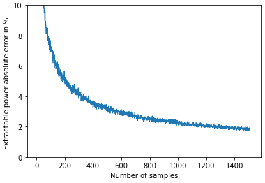
Figure 2 Accuracy of the method of the moment for estimating extractable wind power as a function of the number of samples.

3.5 Correction of low temporal SAR sampling

The main limitation of SAR satellites is their low temporal sampling (one passage every 2 d for Sentinel-1 in Europe). This limitation actually guarantees the statistical independence of measurements. Nevertheless, since SAR satellites are on a sun-synchronous orbit, they always pass at the same time of day, in the morning or in the evening. As a result, they cannot fully see the intraday variability in wind speed. Moreover, the monthly and yearly sampling can also be irregular due to space mission start and end dates and operational constraints.

However, the intraday variability in wind speed is low (Van der Hoven, 1957) and close to a 24 h period sinusoid (Fig. 3). Therefore, since Sentinel-1 satellites pass at two possible times of the day separated by 12 h, according to the Nyquist–Shannon sampling theorem, they should still be able to capture intraday variability. In order to verify this, we computed mean wind speed and extractable wind power using only lidar measurements at 05:00 and 17:00 (UTC). We then compared these results to those obtained using all lidar measurements at any time of day. For all lidar, the differences were found to be below 0.5 % and 1 %, respectively (Table 2). Therefore, SAR satellites are indeed able to capture most wind intraday variability. However, this conclusion might not be true in geographical areas where thermal winds are stronger than in the North Sea.

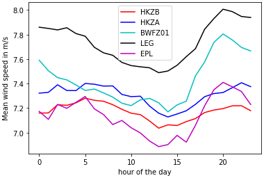
Figure 3 Intraday variability in mean wind speed at 120 m for each lidar. The time is given in UTC, which is close to local time since Zone 1 and Zone 2 are located near the Greenwich meridian (the LEG curve is higher because the campaign was performed during winter).

Table 2 Estimation of mean wind speed error and extractable wind power error due to low temporal SAR sampling.

Figure 4 Relative importance of the input parameters used to correct SAR surface winds.

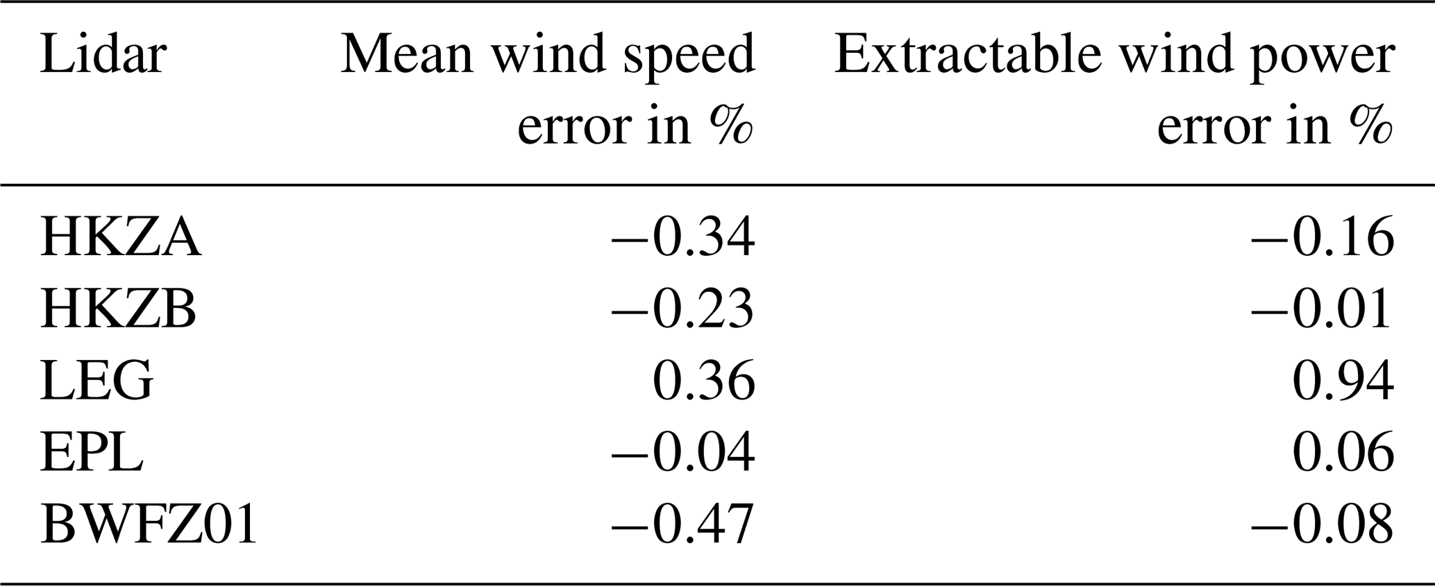
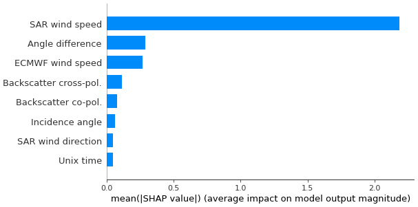
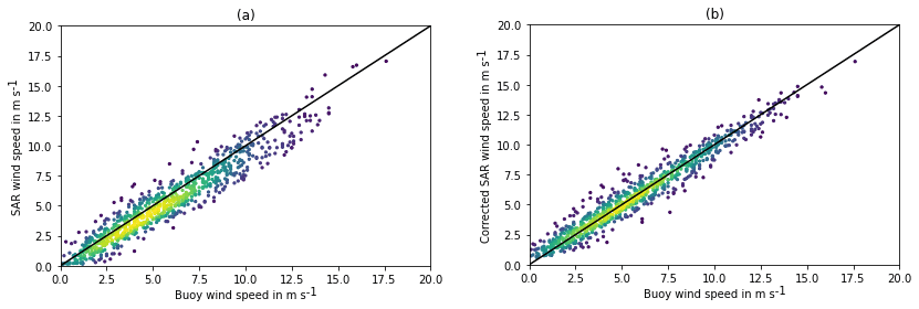
Figure 5 Scatter plots between SAR and buoy wind speeds at 4 $\mathrm{m}\mathrm{a}.\mathrm{s}.\mathrm{l}.$ before machine learning (a) and after machine learning (b) using the test dataset. The colours represent the density of points, and the black curve is the identity line.

Although the effect of intraday variability is expected to be low, in order to improve the accuracy of our method, we decided to correct the errors related to low and irregular SAR sampling. These errors were removed by precisely simulating all of the satellites' passages over the WRF outputs: for each pixel of the study areas, we computed the mean wind speed produced by WRF and compared it to the mean wind speed seen by the satellites. The difference was used to correct SAR mean wind speed.

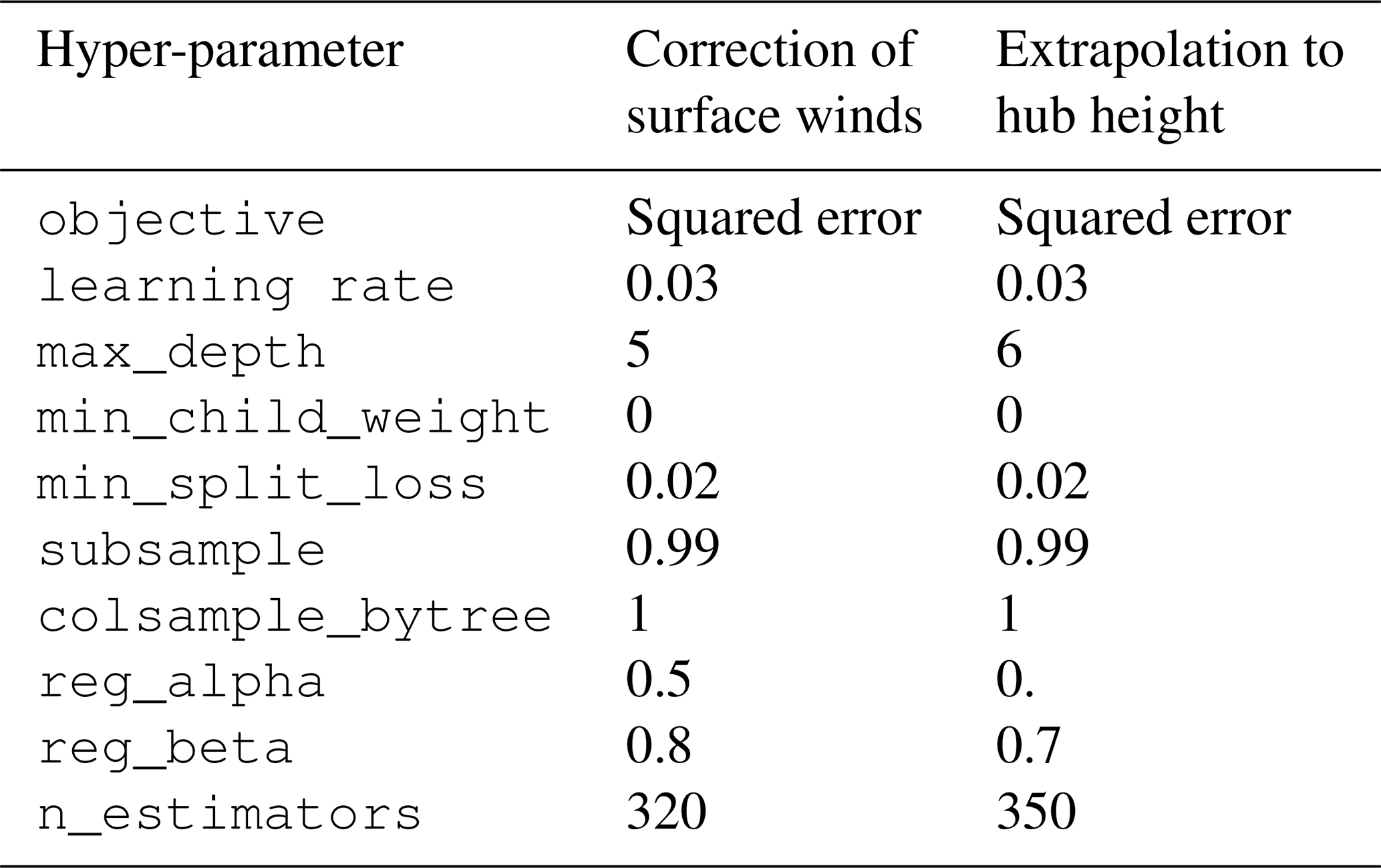
Table 3 Gradient boosting hyper-parameters optimized with grid search with cross-validation.

4 Results

4.1 Performance versus buoys at 4 m

The correction algorithm hyper-parameters optimized with grid search are shown in Table 3 (middle column). The other hyper-parameters are the defaults. The relative importance of the input parameters is given in Fig. 4. As expected, the parameters related to geometry and to low and high wind speeds contained the most useful information. The algorithm was able to reduce the bias in SAR wind speed estimated at 4 $\mathrm{m}\mathrm{a}.\mathrm{s}.\mathrm{l}.$ from −0.48 to 0.02 m s⁻¹, its mean absolute error (MAE) from 0.85 to 0.57 m s⁻¹, and its standard deviation from 0.95 to 0.74 m s⁻¹. Figure 5 shows the scatter plots of SAR wind speeds versus buoys before and after applying machine learning. The bias is indeed reduced and the cloud of points is thinner after machine learning.

Figure 6 Relative importance of the input parameters used to extrapolate SAR surface winds to higher altitudes.

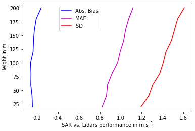
Figure 7 Performance of the machine learning algorithm extrapolating corrected SAR surface winds to higher altitudes.

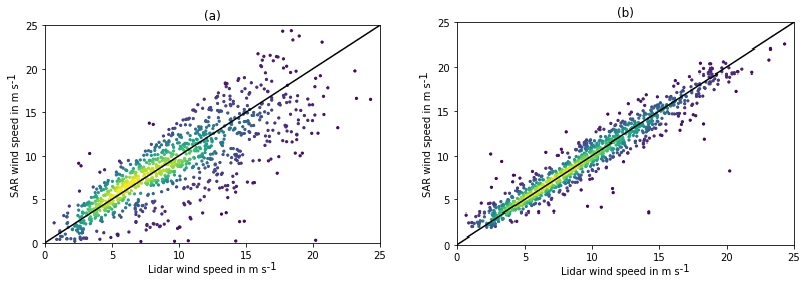
Figure 8 Scatter plots between SAR and lidar wind speeds at 120 $\mathrm{m}\mathrm{a}.\mathrm{s}.\mathrm{l}.$ when the extrapolation is performed with a classical power law (a) or with machine learning (b). The colours represent the density of points, and the black curve is the identity line.

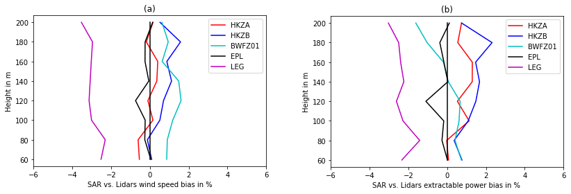
Figure 9 Biases in SAR extrapolated wind speed (a) and extractable wind power (b) versus each lidar as a percentage. The results with LEG lidar are less accurate due to its low number of collocated SAR samples.

4.2 Performance versus lidars

The extrapolation algorithm hyper-parameters optimized with grid search are shown in Table 3 (right column). The relative importance of the input parameters is given in Fig. 6. It can be seen that surface net heat flux was the most relevant atmospheric stability parameter. Algorithm performance versus lidars is shown in Fig. 7 for various altitudes up to 200 m. At 120 m, the hub height of the simulated turbine, the bias in SAR wind speed was 0.16 m s⁻¹, its MAE 0.99 m s⁻¹, and its standard deviation 1.43 m s⁻¹. We also extrapolated corrected SAR wind speeds to higher altitudes, assuming the power law given by Eq. (1) for comparison. Figure 8 shows the scatter plots versus lidars of SAR wind speeds, extrapolated using the power law and machine learning. It can be seen that dispersion was significantly reduced with machine learning. Figure 9 shows the final biases in SAR mean wind speed and SAR extractable power versus each lidar at various altitudes. These biases remained within ± 3 % up to 200 m. As explained previously, an even higher accuracy is expected in real-life industrial applications since the number of samples used here was limited by the short duration of the lidar campaigns used as a reference.

These results need to be confirmed in geographical locations other than the North Sea. Nevertheless, in a region with a very different wind pattern and no available lidar measurements, a simpler method can be applied. The extrapolation ratio provided by the high-resolution numerical model can be used to directly extrapolate SAR surface winds without applying machine learning. In this case, the extractable wind power error was found to be within ± 7 %, which is still accurate enough to provide some insight compared to a numerical model alone.

Figure 10 Wind resource at 120 m over Zone 1, assuming a typical 10 MW turbine: extractable wind power in kilowatts (kW) predicted by WRF (a) and SAR satellites (b), difference in percentage (c), and percentage of low-quality SAR data (d).

Figure 11 Wind resource at 120 m over Zone 2, assuming a typical 10 MW turbine: extractable wind power in kilowatts (kW) predicted by WRF (a) and SAR satellites (b), difference in percentage (c), and percentage of low-quality SAR data (d).

4.3 Wind power maps at hub height

Figures 10 and 11 show the extractable wind power produced at 120 m over the areas of study by the WRF model and SAR satellites and the difference between them as a percentage. It can be seen that the use of SAR data significantly increased the level of detail compared to WRF outputs. In particular, the coastal wind speed gradient, which is often crucial in offshore site assessment, was resolved by the SAR and not by WRF (see the gradients in Fig. 12). Therefore, SAR data can be used to optimize the required distance from the coast and minimize wind farm project risks.

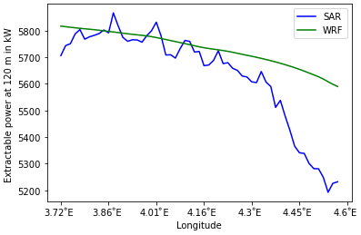
Figure 12 Extractable wind power coastal gradient at 120 m on a horizontal line at the top of Zone 2, estimated by WRF and by SAR satellites.

Some elements are still visible on the maps and need to be corrected in the future. As explained in Sect. 2.2, the presence of these elements was measured using a Koch filter, and a quality flag was created. Figures 10 and 11 also show the percentage of SAR data flagged as “low quality”. These areas were mainly due to bright targets that could not be filtered, related to existing wind farms with a high density of turbines and areas where large numbers of stationary shipping vessels were anchored. In addition, in Zone 1, unrealistic waves can be seen close to the coast. These patterns correspond to similar waves of sand on the seabed. The bathymetry in these shallow waters seemed to affect currents and therefore the SAR backscatter. Regarding swath edges that can still be seen, the problem arises from a difficulty in estimating wind speed standard deviation when the sample number is low. We expect this problem to disappear if more SAR samples are used. In an industrial application, the total number of SAR samples would be between 1000 and 1500, instead of less than 300 as in the worst case here.

5 Conclusion

This article has presented a new method for estimating the offshore wind resource at hub height using SAR and machine learning. The method consisted of three main steps. Firstly, SAR Level-1 products were homogeneously reprocessed into Level-2 surface wind products, and these wind speeds were corrected with a machine learning algorithm using geometrical parameters of the SAR sensor and SAR metadata to compensate for systematic errors attributed to the GMF or SAR calibration. This algorithm was trained with a large network of weather buoys. Secondly, SAR surface winds were extrapolated to higher altitudes with another machine learning algorithm, using meteorological parameters extracted from a high-resolution numerical model. This algorithm was trained with a dataset of lidar vertical wind profiles. Thirdly, the wind speed Weibull parameters were estimated, taking into account SAR irregular sampling, and a wind turbine was simulated to compute the extractable wind power computed.

This first machine learning algorithm correcting SAR surface wind speeds was tested against 4 m high buoy measurements. The resulting SAR wind speed bias was 0.02 m s⁻¹. Its MAE was 0.57 m s⁻¹ and its standard deviation 0.74 m s⁻¹. This algorithm can be used stand-alone to improve the accuracy of SAR wind products. The second algorithm extrapolating surface winds to higher altitudes was tested against lidar measurements up to 200 m. At 120 m, which is the hub height of the simulated turbine, the extrapolated wind speed bias was 0.16 m s⁻¹. Its MAE was 0.99 m s⁻¹ and its standard deviation 1.43 m s⁻¹. This algorithm can also be used stand-alone to extrapolate wind speeds measured at 4 $\mathrm{m}\mathrm{a}.\mathrm{s}.\mathrm{l}.$ These two algorithms combined together produced instantaneous SAR wind fields at hub height, which can provide interesting insights for wind farm developers. When these SAR wind speeds at hub height were converted into potential extractable wind power, at 120 m, the accuracy was 3 % versus lidars. Since this assessment was done with a low number of SAR samples due to the limited duration of lidar campaigns, higher accuracy is expected in an industrial application.

The method was tested in two areas off the Dutch coast. Compared to the maps provided by the WRF numerical model, this method has the advantage of providing a much higher level of detail thanks to the 1 km resolution provided by SAR surface wind measurements. The most striking result is that wind resource maps based on SAR were able to resolve the wind speed coastal gradient. Therefore, using SAR data combined with machine learning can improve the accuracy of offshore wind resource estimates at hub height and provide useful insights to optimize wind farm siting and risk management.

Further research should focus on removing remaining artefacts on SAR maps, such as swath edges, bright targets, and the effect of bathymetry. Moreover, since the method was validated using lidars located only in the North Sea, the extrapolation algorithm may not be adapted to meteorological conditions in seas with a different wind climate. In these cases, wind profiles measured by lidars located in the region of interest would need to be included in the training dataset and used to validate the method again.