the Creative Commons Attribution 4.0 License.
the Creative Commons Attribution 4.0 License.
 | 10 Oct 2022
Wind turbine wake simulation with explicit algebraic Reynolds stress modeling
Stefan Wallin
Maarten Paul van der Laan
Mark Kelly
Reynolds-averaged Navier–Stokes (RANS) simulations of wind turbine wakes are usually conducted with two-equation turbulence models based on the Boussinesq hypothesis; these are simple and robust but lack the capability of predicting various turbulence phenomena. Using the explicit algebraic Reynolds stress model (EARSM) of Wallin and Johansson (2000) can alleviate some of these deficiencies while still being numerically robust and only slightly more computationally expensive than the traditional two-equation models. The model implementation is verified with the homogeneous shear flow, half-channel flow, and square duct flow cases, and subsequently full three-dimensional wake simulations are run and analyzed. The results are compared with reference large-eddy simulation (LES) data, which show that the EARSM especially improves the prediction of turbulence anisotropy and turbulence intensity but that it also predicts less Gaussian wake profile shapes.
- Article
(10018 KB) - Full-text XML
- BibTeX
- EndNote


As wind farms increase in size and number of turbines, increasingly more attention should be given to the study of wind turbine wakes, as they can account for a relatively large power production decrease. Simple engineering models, such as the classic Jensen (1983) model, the “new-classic” Bastankhah and Porté-Agel (2014) model, or the more recent Ishihara model (Ishihara and Qian, 2018), can be used to model the flow through a wind farm on a regular laptop in a matter of seconds. However, they all share some common weaknesses: they are based on rather strict flow assumptions, need empirically tuned parameters, and require a superposition model for overlapping wakes.
A wind turbine wake is a complex three-dimensional swirling flow, and its development is governed by turbulent mixing, which is strongly influenced by density stratification in the atmospheric boundary layer (ABL) and the interaction between the ABL and the wake itself. To model a more physically correct wind farm flow we therefore solve the Navier–Stokes equations, which in essence are a reformulation of Newton's second law, along with conservation of mass. The process of discretizing and solving these equations on computers is known as computational fluid dynamics (CFD). Unfortunately, the Reynolds number of atmospheric flows is so large (106–108 or more; see, e.g., Wyngaard, 2010) that it is unfeasible to conduct direct numerical simulation (DNS) for even a single-wind-turbine wake. Instead large-eddy simulation (LES), i.e., the simulation of the spatially filtered Navier–Stokes equations, has been performed by numerous groups in the last decade; see review by Breton et al. (2017). Even though the rotor geometry is reduced to an actuator disk (AD) or an actuator line (AL) model, these simulations require a vast number of CPU hours on modern high-performance computing (HPC) clusters, again even for a single-wind-turbine wake. A much faster simulation can be conducted by solving the Reynolds-averaged Navier–Stokes (RANS) equations instead; however, in contrast to LES, which needs only to parameterize turbulent fluctuations at the smallest (unresolved) scales, RANS simulation relies heavily on the quality of the turbulence model because it must model fluctuations across all simulated scales. For example, the standard two-equation k–ε model of Launder and Spalding (1974) was shown by Réthoré (2009) to perform poorly for simulation of wind turbine wakes in terms of wake recovery prediction and also generating unphysical Reynolds stresses in the vicinity of the turbine (i.e., unrealizable turbulence). This is not unexpected since it was originally developed for simple free shear and boundary layer flows, e.g., flat plate, pipe, plane jet, and cavity flows (Launder and Spalding, 1974). The standard k–ε model is considered to be a linear eddy viscosity model (EVM) because the anisotropy tensor, (where is the Reynolds stress tensor; k is the turbulent kinetic energy, TKE; and δij is the Kronecker delta tensor), is linearly proportional to the normalized strain rate tensor through the Boussinesq hypothesis (Boussinesq, 1897); see also Eq. (5). A modified model coined the “k–ε–fP” model was developed and calibrated specifically for atmospheric wind farm flows by van der Laan (2014), and it showed much improvement over the standard k–ε model. It is essentially equivalent to the first-order model of the non-linear eddy viscosity model (NLEVM) of Apsley and Leschziner (1998).
Linear EVMs based on the Boussinesq hypothesis (e.g., mixing length, k–ε and k–ω models) are the de facto standard for RANS in many fields of research, including wind energy applications (e.g., Bleeg et al., 2018; Hornshøj-Møller et al., 2021; Heinz et al., 2021; Dicholkar et al., 2022; Letizia and Iungo, 2022). They are simple to implement and numerically robust but have a drawback in terms of physical correctness – the example of wake recovery has already been mentioned earlier, and one can also quickly derive that the Reynolds stresses become unrealizable for large normalized strain rates in general; see Fig. 2. Full Reynolds stress modeling (RSM), where a transport equation for each of the six unique Reynolds stress components is solved, was conducted by Launder et al. (1975), and this approach leads to more physical predictions because one avoids the use of the quite limiting Boussinesq hypothesis, and hence the production of turbulence needs no further modeling, which is a major improvement. The drawback of this method is that it is more computationally expensive and, perhaps more importantly, less numerically stable. Rodi (1976) deployed the weak equilibrium approximation (WEA) to the RSM equations, which transforms the set of differential equations into a set of algebraic equations while still retaining most of the physical behavior of the RSM. This approach is known as the algebraic Reynolds stress model (ARSM), and it can be formulated as a tensor equation for the anisotropy tensor, but unfortunately it is a non-linear implicit equation with multiple solutions, which is also prone to numerical stability issues. Pope (1975) simplified the ARSM by using the Cayley–Hamilton theorem and obtained the first explicit algebraic Reynolds stress model (EARSM) for the case of two-dimensional flow, which as the name suggests is an explicit algebraic relation between the Reynolds stress tensor (or equivalently the anisotropy tensor) and the normalized strain rate and rotation rate tensors. Different three-dimensional generalizations were subsequently made by Taulbee (1992), Gatski and Speziale (1993), and Wallin and Johansson (2000), which differ in the constants and more importantly in the way they treat the non-linearity of the ARSM. The Wallin and Johansson (2000) EARSM (hereafter WJ-EARSM) is chosen for this work because it is based on the concept of self-consistency (meaning that the explicit solution of aij satisfies the non-linear ARSM tensor equation exactly in two-dimensional mean flows and approximately in three-dimensional mean flows) and is only slightly more computationally expensive compared to a standard k–ε model. The self-consistent solution was independently formulated by Girimaji (1996), Ying and Canuto (1996), and Johansson and Wallin (1996) and facilitates a consistent solution in non-equilibrium conditions (where TKE production does not balance dissipation of TKE).
It appears that only Gómez-Elvira et al. (2005) and van der Laan (2014) have attempted to use EARSM for RANS simulations of wind turbine wakes. Many other research areas have however used the WJ-EARSM successfully (e.g., airfoil flow, Franke et al., 2005; vortex generators, Jirásek, 2005; stirred tanks, Feng et al., 2012; Kaplan turbines, Javadi and Nilsson, 2017; and high-speed trains, Munoz-Paniagua et al., 2017), so it seems that an untapped potential exists in turbulence modeling for wind energy applications. Gómez-Elvira et al. (2005) deployed the Taulbee (1992) model in a parabolic RANS setup, which is fast to execute but lacks physical features such as the upstream induction zone; van der Laan (2014) tested the Taulbee (1992), Gatski and Speziale (1993), and Apsley and Leschziner (1998) models in the elliptic RANS solver EllipSys3D (Sørensen, 1995) but found that they were more numerically unstable compared to the standard k–ε model.
The EARSM framework of Wallin and Johansson (2000) has been further exploited by including the strong coupling with density stratification present in the ABL (Lazeroms et al., 2013), capturing the effect of both stable and convective ABLs (Lazeroms et al., 2016; Želi et al., 2020, 2021). In this paper, we restrict the study to the neutral atmospheric surface layer (ASL; i.e., the lower part of the ABL), leaving stratified conditions for upcoming studies.
Section 2 describes the turbulence model formulations. In Sect. 3, we verify our implementation of the WJ-EARSM using several canonical flow cases, and finally in Sects. 4 and 5, it is applied to simulations of wind turbine wakes in the neutral ASL.
The turbulence models utilized in this paper assume incompressible, non-stratified flow; no system rotation (no Coriolis or centrifugal contributions); isotropic dissipation of TKE; and high Reynolds number flow.
2.1 The standard k–ε model (Launder and Sharma, 1974)
The Boussinesq hypothesis is used to obtain the Reynolds stresses
which are needed to close the momentum equations (the equations for the mean velocity vector, Ui). The eddy viscosity in a linear EVM is defined as , and transport equations are used to obtain TKE (k) and dissipation of TKE (ε):
This paper focuses on the k–ε model because it is traditionally used for atmospheric flows (e.g., Crespo et al., 1985; Richards and Hoxey, 1993; Sørensen, 1995), but the widely used k–ω model could as well have been used. They can both be categorized as linear EVMs because they use the Boussinesq hypothesis to obtain the Reynolds stresses. Several empirical constants are also present for both models, though they are related to each other (Sogachev and Kelly, 2012); for the k–ε model there are Cμ, σk, Cε1, Cε2, and σε (see review by Weaver and Mišković, 2021, for the most popular sets of constants used in the past). We shall use different sets of constants throughout the paper and remark the choice at each usage of the k–ε model.
To simplify the Boussinesq hypothesis, Eq. (1), we can use the anisotropy tensor also mentioned in the introduction:
It is dimensionless, symmetric, and traceless, and Eq. (1) can then be re-written as
where is the normalized strain rate tensor. The k–ε model is independent of the normalized rotation rate tensor, ; hence it will be unable to predict turbulence effects associated with rotation or curvature, e.g., damping/enhancement of turbulence in rotating homogeneous shear flow (Wallin and Johansson, 2002). The more advanced EARSMs also need to solve the k and ε transport equations because they depend on Sij and Ωij and hence depend on the turbulence timescale . The key difference between these more advanced models and the standard k–ε closure is that the Boussinesq hypothesis is replaced by a more general constitutive relation.
Finally, it can be noted that the time derivative is retained in the transport equations, Eqs. (2)–(3), to allow for unsteady RANS (URANS) simulations, e.g., homogeneous shear flow. URANS is generally only advisable when there is a clear separation between the timescale of the turbulence and the mean unsteadiness (see, e.g., Wallin, 2000) and should therefore be used with care.
2.2 The k–ε–fP model
The k–ε–fP model by van der Laan (2014) is equivalent to the first-order model of Apsley and Leschziner (1998), except for a re-tuning of the model coefficients. To summarize,
Compared with the Boussinesq hypothesis, Eq. (5), we see that the only difference is that the k–ε–fP model uses a variable or “effective” , which is flow-dependent and thereby makes aij non-linear in the velocity gradient tensor; however, the k–ε–fP model is still referred to as a “linear EVM” (e.g., van der Laan, 2014) because the direction of aij is aligned with Sij and not any other higher-order tensors. The fP function is
In the above equation σ is the “shear parameter”, which can be re-written using velocity gradient tensor invariants (see Eq. 14), while is the shear parameter of the freestream calibration flow. Instead of using DNS channel flow data for the calibration, as was done by Apsley and Leschziner (1998), van der Laan (2014) chose to calibrate with a neutral ASL (logarithmic wind profile), which simply gives . Finally, van der Laan (2014) took the Rotta constant as a free parameter and tuned it to CR=4.5 using LES data of wake velocity and TI (pressure-strain data were not used) extracted from eight different wind turbine wake cases.
In the freestream of a neutral ASL, fP=1, so it reduces to the standard k–ε model, while fP<1 in regions with rapid strain compared to the turbulence timescale (i.e., large normalized velocity gradients), hence attenuating mixing in the wake shear layers and improving predictions of wind turbine wakes as found by van der Laan (2014). The fP correction reduces mainly the turbulence length scale (but also the turbulence velocity scale) in the near wake and can therefore be interpreted as a local turbulence-length-scale limiter, as discussed by van der Laan and Andersen (2018). In fact, the damping introduced through fP will preserve realizability for rapid shear (large normalized velocity gradient); i.e., in the rapid distortion theory (RDT) limit it will predict , whereas the standard k–ε model would predict (unrealizable turbulence); see Fig. 2.
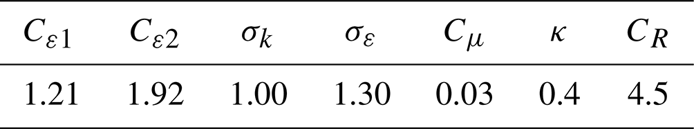
Table 1 summarizes the model constants of the k–ε–fP model, where one can notice that Cμ=0.03 is used instead of the established value of Cμ=0.09 (e.g., Launder and Spalding, 1974). Several measurements of atmospheric flow in flat terrain (e.g., Panofsky and Dutton, 1984) point to a lower Cμ, and Bottema (1997) argues that this is due to “inactive” low-frequency atmospheric turbulence; see also discussion by Richards and Norris (2011). As a compromise is used in WAsP-CFD (Bechmann, 2016).
Table 1Model constants for the k–ε–fP model as recommended by Sørensen (1995) and van der Laan (2014). Referred to later as “ABL coefs”.
2.3 Wallin and Johansson (2000) EARSM
The EARS model of Wallin and Johansson (2000) is derived from the ARSM of Rodi (1976) and therefore inherits the constants, c1 and c2, which are the Rotta coefficient and rapid pressure-strain coefficient of the Launder et al. (1975) model, respectively. The particular choice reduces the model expressions significantly and is adopted in this study. This choice is also supported by the DNSs of Shabbir and Shih (1993). Moreover, we only consider the incompressible, high-Reynolds-number version (without near-wall corrections) due to the high Reynolds number and the use of rough-wall function boundary conditions at the ground in the considered flow cases of this paper. Additionally, we make comparisons between the 2D and 3D models. It is important to stress that the 2D model is fully general and invariant and can be used for simulation of three-dimensional mean flows as noted by Hellsten and Wallin (2009); this has for example also been commonly done with the EARSM of Gatski and Speziale (1993). Another important point to mention again is that all EARSMs are based on combinations of Sij and Ωij (which depend on the turbulence timescale, ), so one still needs to solve either the k–ε model (used in this paper), k–ω model (used by Wallin and Johansson, 2000), or some other combination for obtaining the turbulence timescale.
2.3.1 2D WJ-EARSM
Using the complete two-dimensional tensor basis for the anisotropy tensor (Pope, 1975), an exact self-consistent 2D EARSM was found independently by Johansson and Wallin (1996), Girimaji (1996), and Ying and Canuto (1996). It was more thoroughly elaborated and tested by Wallin and Johansson (2000), where derivation details also can be found. Without loss of generality, and for the reason of numerical implementation, the anisotropy is split into linear and “extra” terms:
where
The tensor coefficients are
while N is the real and positive root of a cubic polynomial related to the non-linearity of the EARSM:
The model only depends on the first two velocity gradient tensor invariants:
The solution procedure is more thoroughly described in Sect. 2.4, but one can just notice that given Sij and Ωij, there is a closed and explicit solution of aij. Since N, Eq. (12), is an exact solution of the underlying cubic polynomial problem, aij is an exact solution of the ARSM; hence it is a self-consistent EARSM, which ensures good model predictions in non-equilibrium conditions for . We suspect that the treatment of the EARSM non-linearity by Taulbee (1992), Gatski and Speziale (1993), and Apsley and Leschziner (1998) is one of the main causes for the numerical instability when these EARSMs/NLEVMs are employed to model wind turbine wakes (van der Laan, 2014).
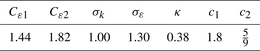
Cμ is not an input parameter but an output parameter as a result of applying the WJ-EARSM; see Eq. (9). However, one still needs it for the rough-wall boundary condition (BC) used in our code and for the diffusion terms in the k and ε transport equations in our implementation; here we shall use Cμ=0.087, which is the equilibrium value (the value obtained by fixing and considering the log-layer relations) with the current set of constants in Table 2; see Sect. 4.1. Also note that κ=0.38 is not an input parameter but is calculated from the other model constants in order to satisfy the log-layer balance; see Eq. (23).
Table 2Model constants for the WJ-EARSM as recommended by Želi et al. (2020). Referred to later as “Zeli coefs”.
2.3.2 3D WJ-EARSM
The 3D model is derived in an analogous way to the 2D model (Wallin and Johansson, 2000) but with the complete three-dimensional tensor representation of aij, which gives
with
The tensor coefficients and basis tensors are
| , | |||
where
Unfortunately, there does not exist an analytical solution for N in the 3D model; therefore the cubic N solution from 2D, Eq. (12), is used; hence the 3D model is not exactly self-consistent, but the cubic N solution is however still a quite good approximation in many cases. The same model constants are also used; see Table 2.
One can show that the 3D model reduces to the 2D model in two-dimensional mean flows, where , IV=0, and are valid.
2.4 Implementation details
The flow cases are simulated with EllipSys3D, which is a finite-volume CFD solver developed and described in detail by Michelsen (1992) and Sørensen (1995). The solver already has implementations of the standard k–ε model and the k–ε–fP model (van der Laan, 2014), so the following focuses on the implementation of the WJ-EARSM. As emphasized in the previous sections, both the 2D and 3D models can be written in the same form; see Eqs. (8) and (15) (although with different expressions for and ). The splitting of the anisotropy tensor into a linear and an extra part makes the implementation relatively straightforward in codes that already have a k–ε model implemented, as also noted in Appendix A of Wallin and Johansson (2000); for the momentum equations, simply use instead of , and add as a source term:
For numerical stability, it is recommended to include the first term in the system matrix and the second term in the source vector (i.e., treat the terms implicitly and explicitly, respectively). The third term is isotropic and can be absorbed into a modified pressure.
In the k and ε transport equations, we use the standard νt in the diffusion terms (𝒟(k) and 𝒟(ε) in Eqs. 2–3) since these are calibrated using the standard model. This practice is also used by Apsley and Leschziner (1998), Myllerup (2000), and Menter et al. (2009). In the original paper of Wallin and Johansson (2000), it was proposed to use the Daly–Harlow diffusion model or an eddy-diffusion model with the effective , which was later abandoned for the standard eddy-diffusivity model (see, e.g., Menter et al., 2012). The TKE production is calculated consistently as with the full anisotropy tensor; this expression is in fact valid for all turbulence models (see for example Wallin and Johansson, 2000).
A segregated solver (i.e., solving the U equation, then the V equation, then the W equation, etc.) is used in EllipSys, and the same shear production 𝒫 is used in both turbulence transport equations; an overview of the procedure is sketched in Fig. 1. The boundary conditions for each variable depend on the type of boundary (rough wall, inlet, outlet, cyclic, or symmetric), and the implementation of these in EllipSys3D is described by Sørensen (1995) and Sørensen et al. (2007).
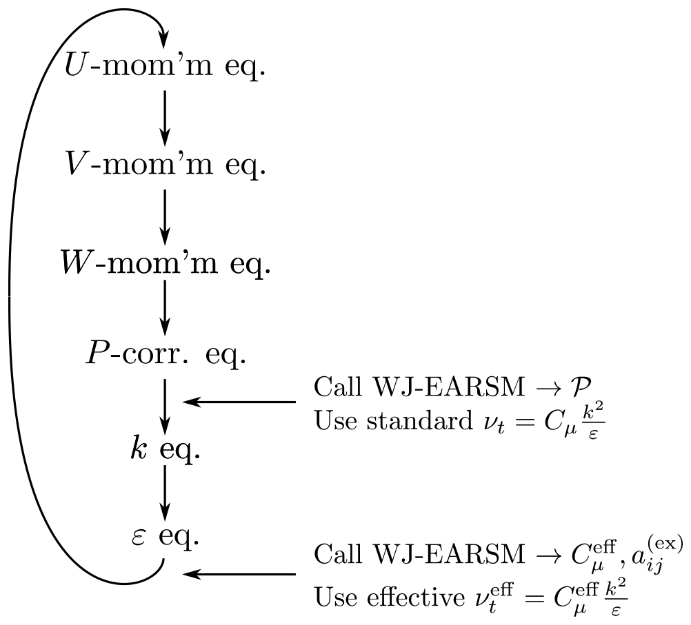
Figure 1Segregated solver procedure for WJ-EARSM in EllipSys3D. Note that P is the mean pressure, while 𝒫 is the TKE shear production.
The 1D version of EllipSys3D, EllipSys1D (van der Laan and Sørensen, 2017), is used for the 1D verification cases in Sect. 3. Its code structure is very similar to EllipSys3D's, but it has no W momentum equation (W=0) and no pressure correction equation (, so continuity is ensured already), and it is written using 1D simplifications (mean variations only in time and z direction), which makes it possible to run 1D simulations, or so-called “single-column models”, on a regular laptop in a few seconds.
For both EllipSys1D and EllipSys3D, the procedure of calling the WJ-EARSM is as such:
-
Use the most recent solution of momentum and turbulence transport equations to calculate the normalized strain rate and rotation rate tensors, Sij and Ωij.
-
Calculate tensors and invariants.
-
Calculate N.
-
Calculate coefficients, β1, …, β10.
-
Calculate anisotropy tensor, aij.
-
Calculate TKE shear production, .
-
Calculate and .
As is clear from the previous section, the expressions in the WJ-EARSM are considerably longer compared to the ones of the k–ε and k–ε–fP models. Three canonical flows (homogeneous shear flow, half-channel flow, and square duct flow) are therefore used as verification cases to gain confidence in the numerical implementation (verification is the process of ensuring correct implementation, whereas validation is the process of assessing a model's accuracy; see Réthoré et al., 2014); full three-dimensional wind turbine wake simulations are first considered in Sect. 4. The first two cases can be simulated in a 1D setup, which make them ideal for initial testing, while the last case needs to be simulated in 3D due to the phenomenon of secondary motions. For the latter, a quasi-2D setup – homogeneous in the streamwise direction – would be possible, but a fully three-dimensional setup is chosen for verification of the 3D implementation. All cases are compared to either analytic expressions or DNS data to verify correct behavior of the implementation.
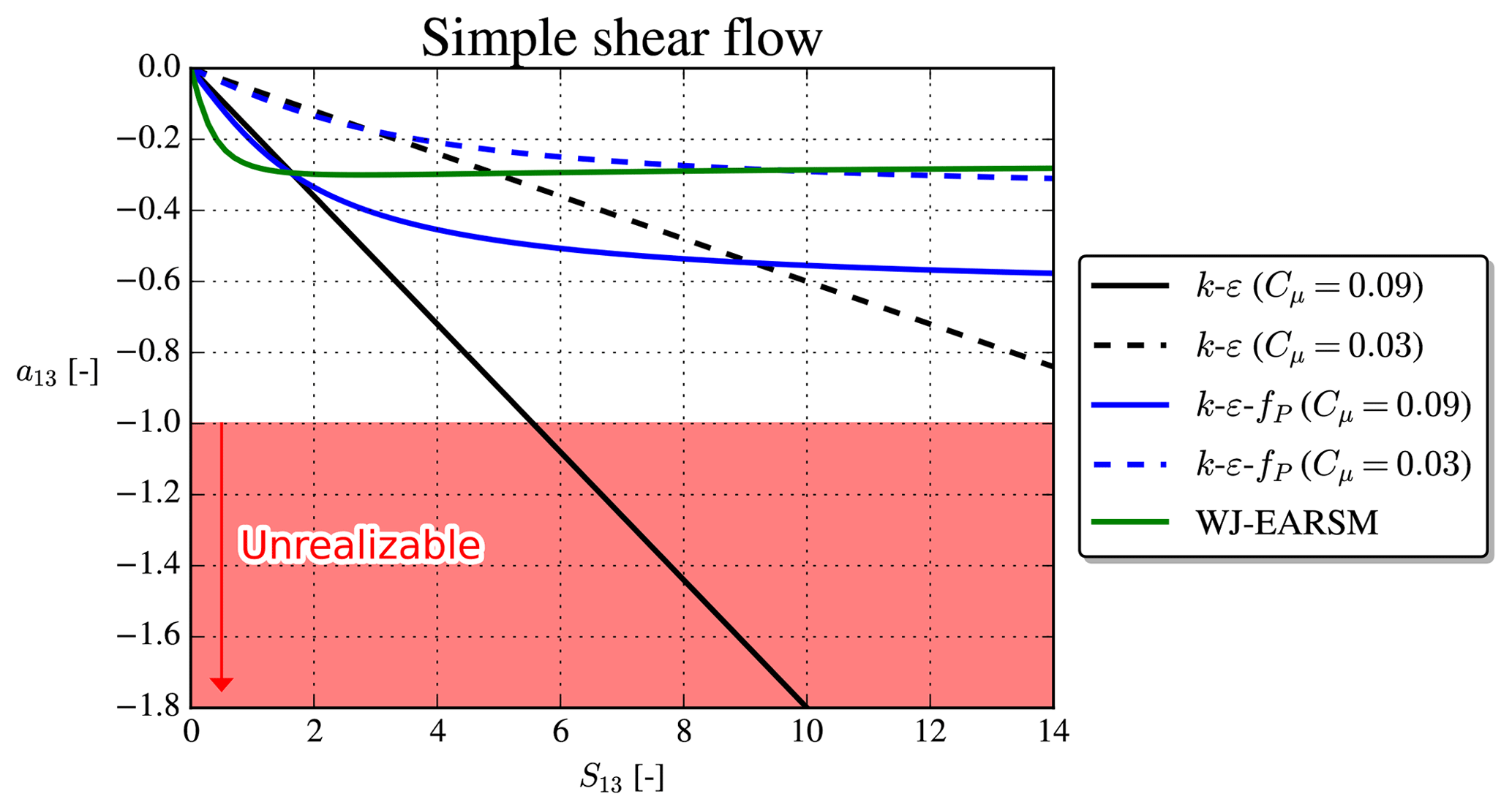
Even before running the verification cases, we consider the general class of “simple shear flows” (a.k.a. 1D parallel flows), where the normalized strain rate and rotation rate tensors are
Prescribing S13 enables us to evaluate the turbulence models analytically and obtain the anisotropy tensor, aij. The a13 component is shown in Fig. 2, and from the Cauchy–Schwarz inequality one can show generally that ; if a turbulence model violates this, then it predicts “unrealizable” turbulence, meaning unphysical turbulence. For large S13, the k–ε model leads to unrealizable turbulence, while both the k–ε–fP model and WJ-EARSM (the 2D and 3D WJ-EARSMs are identical in 1D) are realizable even for large S13. This is very desirable because large normalized velocity gradients are typically encountered in regions of non-equilibrium turbulence, e.g., in the vicinity of the rotor and in the wake shear layers. Indeed Réthoré (2009) noted large regions of unrealizable turbulence near the wind turbine when using the standard k–ε model. Also note that the k–ε–fP model (using Cμ=0.03) predicts a similar a13 as the WJ-EARSM solution for large strains, while the main difference between the models is found for small strains.
3.1 Homogeneous shear flow
Homogeneous shear flow (see review by Pope, 2000, pp. 154–157) has a simple setup but can be challenging to simulate and is conceptually a strange case. The momentum equations are not solved, and instead a constant velocity gradient is artificially fixed at all times; see Fig. 3. This is, indeed, rather unphysical since the velocity gradient should gradually decrease as turbulence is created until the velocity gradient eventually becomes zero, and turbulence dies out. Nevertheless, homogeneous shear flow constitutes an interesting test case because it only involves the solution of the turbulence transport equations and turbulence closure; hence it is a “pure” test of the turbulence model. Moreover, free-shear layers can locally be approximated with homogeneous shear. Only EllipSys1D is used for this case.
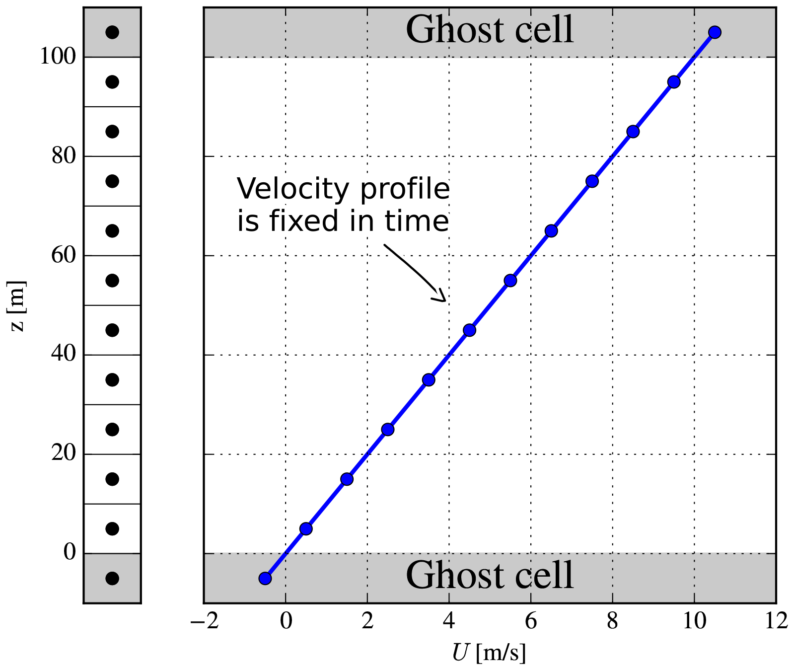
Figure 3Mesh and the prescribed velocity profile in EllipSys1D for the homogeneous-shear-flow case.
In principle, homogeneous shear flow is an unsteady 0D case. The turbulence evolves identically at all positions in space; hence there is actually no need for a spatial discretization as shown in Fig. 3 (one could simply integrate the k and ε equations forward in time, given an initial turbulent state, as done by for example Taulbee, 1992), but this extra complexity is chosen for the present case since the goal is to verify the turbulence model implemented in a finite-volume CFD code. In practice this means that BCs need to be set at the top and bottom of the domain: a fixed velocity, U, is used as illustrated in Fig. 3, while symmetry BCs are used for k and ε. The implicit Euler scheme is used for time integration, while the second-order central scheme is used for diffusive terms.
The simulation parameters used are as follows.
-
Height of domain, Lz=100 m. Uniform spacing and 10 finite-volume cells are used (if ghost cells are counted in, there are 12 cells); hence grid spacing is Δz=10 m.
-
Fixed velocity profile, U(z)=Sz, where S=0.1 s−1. This gives and U(Lz)=10 m s−1.
-
Normalized time step, (in physical time Δt=1 s). Ten subiterations per time step are used, and the total normalized simulation time is (in physical time t=800 s).
-
Initial turbulent state, at . This non-dimensional quantity determines the evolution of the non-dimensional metrics, i.e., anisotropy components, production-to-dissipation ratio, etc.; it is the same initial turbulent state as used in the homogeneous shear flow simulations by Bardina et al. (1983), Gatski and Speziale (1993), Girimaji (1996), and Wallin and Johansson (2002).
The RANS model equations here are independent of ρ and ν because no momentum equation is solved, and the diffusion terms in the k and ε equations (𝒟(k) and 𝒟(ε)) in Eqs. (2)–(3) will be zero.
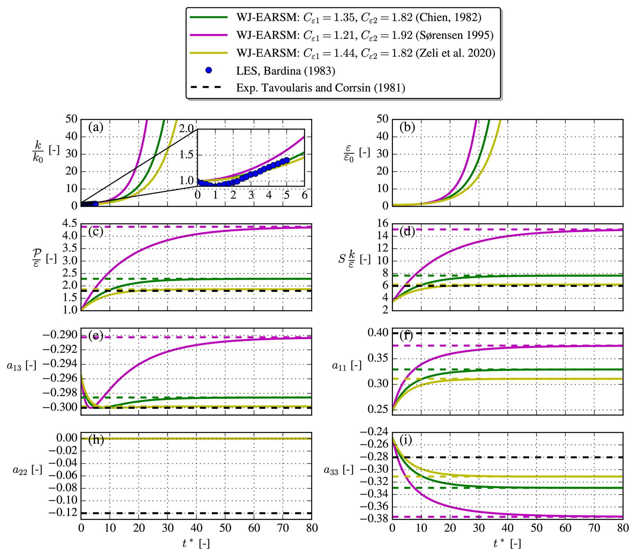
Figure 4Simulation of homogeneous shear flow with WJ-EARSM (full line) and the model's analytical asymptotic values (dashed lines) with different sets of constants. The simulation data are extracted at , but the evolution is identical at all grid points.
A nice feature of homogeneous shear flow for verification purposes is that it evolves to an asymptotic state and that an analytic solution exists for this state; e.g., the asymptotic production-to-dissipation ratio can be derived to be (see for example Gatski and Speziale, 1993)
Table 3Analytic, asymptotic homogeneous shear flow formulas. In homogeneous shear flow, , while all other components are 0. When is known, one can use the direct definition of instead of Eq. (12); see Wallin and Johansson (2000).
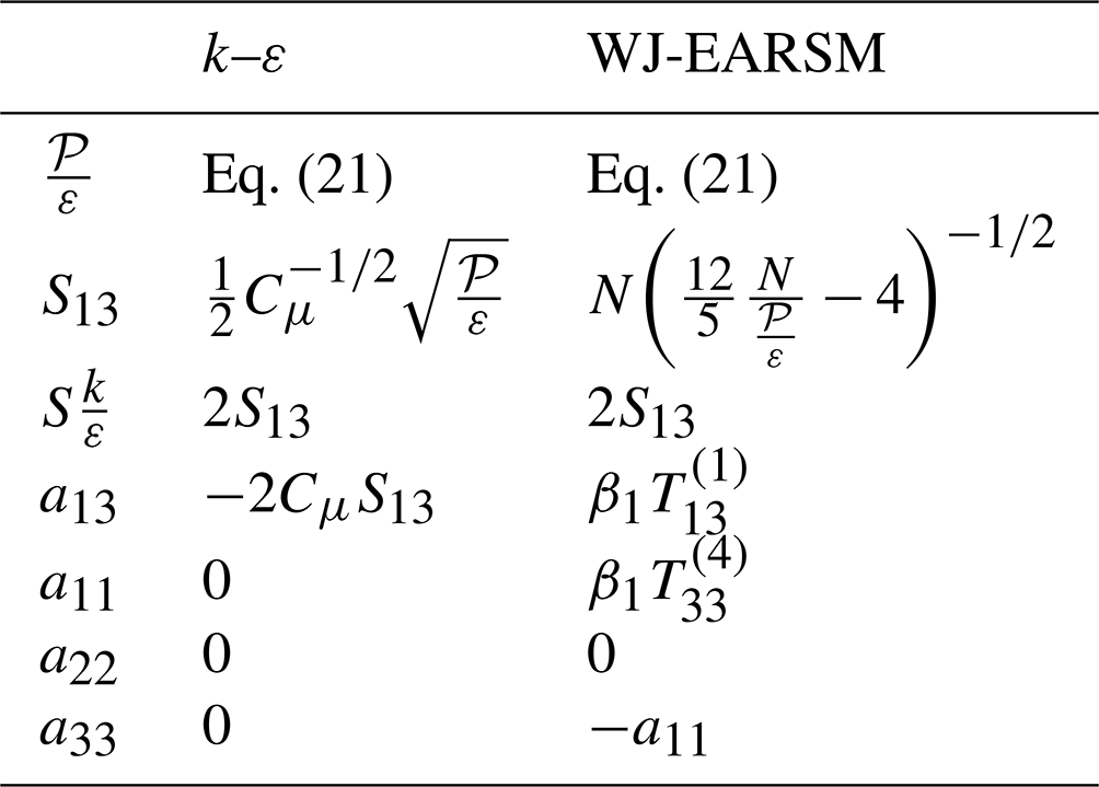
In 1D parallel flows, , and this gives a second equation for . By inserting the expression for a13 (the expression differs depending on the turbulence model), one can isolate and obtain a value for . This value can then be used to obtain Sij and Ωij and hence the anisotropy tensor. The asymptotic formulas are summarized in Table 3, where one can note that the asymptotic WJ-EARSM formulas only depend on Cε1 and Cε2, while the k–ε formulas additionally depend on Cμ. Figure 4 shows the time evolution of the WJ-EARSM as well as the theoretical asymptotic values for three common sets of coefficients (Cε1, Cε2). All simulations indeed go to the analytical asymptote, which gives some confidence in the implementation of the WJ-EARSM. For validation purposes we also include some LES (Bardina et al., 1983) and experimental (Tavoularis and Corrsin, 1981) data in Fig. 4, which show that the Zeli constants perform better for all quantities except a11. The choice of makes a22=0 for all simulations.
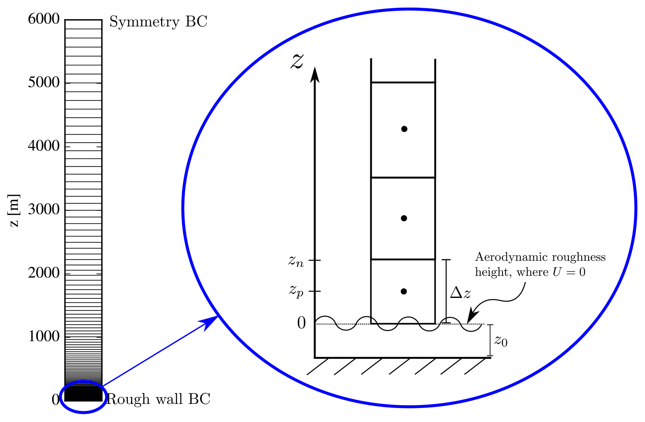
Figure 5Half-channel EllipSys1D setup. The sketch to the right shows the convention of the coordinate system used for rough-wall simulations.
3.2 Half-channel flow
The second reference flow is the fully developed, steady-state half-channel flow, a.k.a. pressure-driven boundary layer (PDBL) flow, and can be solved in 1D using a grid as sketched in Fig. 5. The lower BC is a rough wall implemented as in Sørensen et al. (2007), while the upper BC uses symmetry; hence turbulence now depends on the z coordinate contrary to in the homogeneous-shear-flow case. The flow is driven by a constant streamwise pressure gradient force, which is an input parameter for the simulation (if one does not use such a forcing, then the rough wall will extract momentum from the flow, and the velocity eventually becomes zero throughout the domain).
The input parameters for the simulations are as follows:
-
Height of domain, Lz=6000 m. The grid is stretched using the hyperbolic tangent function (Thompson et al., 1985), and 192 finite-volume cells are used (if ghost cells are counted in, there are 194 cells).
-
Aerodynamic roughness height, z0=0.03 m. This is used for the rough-wall BC in the first wall-adjacent cell, which has a height of Δz=0.10 m.
-
Streamwise pressure gradient force per unit mass, m s−2. One can show that the squared friction velocity then becomes m s−1.
The flow is independent of ν because a rough-wall BC is used and the flow is fully turbulent, hence ν≪νt.
The region in the lower part of the domain is known as the “log layer”, which is characterized by equilibrium turbulence, i.e., . As in the homogeneous-shear-flow case, we can use this ratio to obtain analytical results for shear and anisotropy; see Table 4.
Table 4Analytical values in the log layer of the half-channel flow.
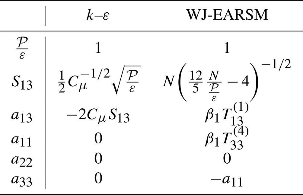
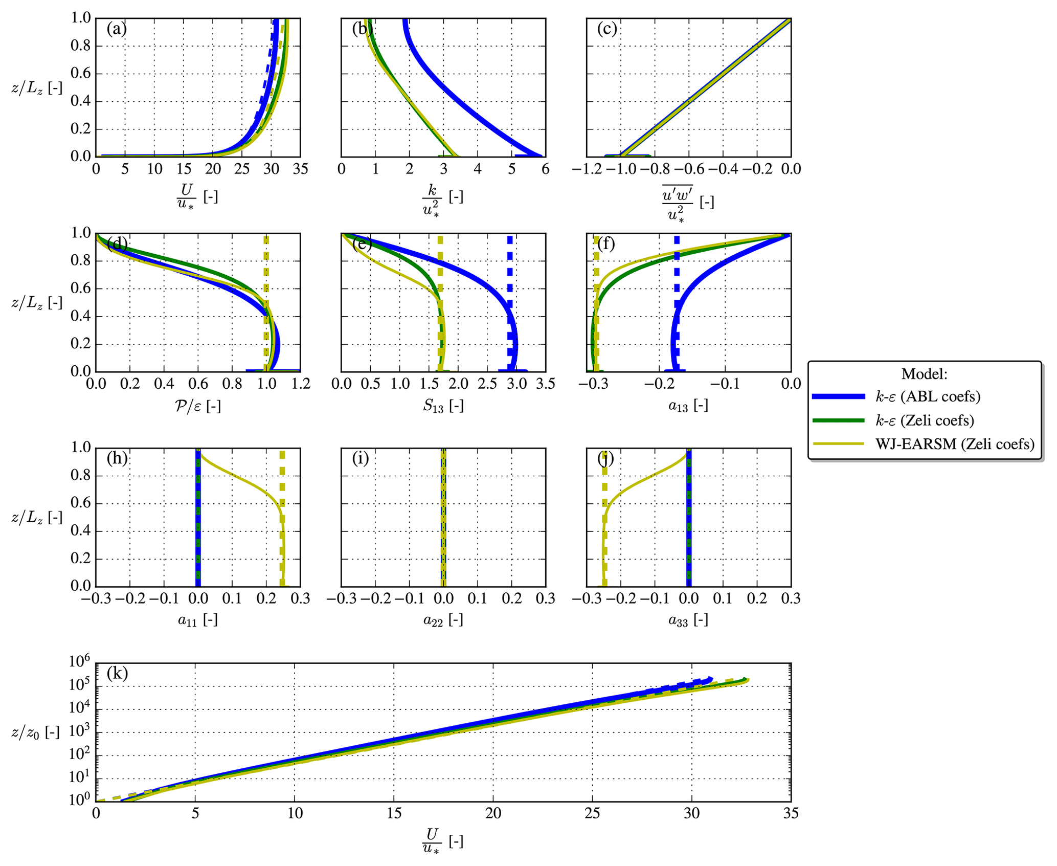
Figure 6Half-channel simulation results (full lines) and analytical log-layer solutions (dashed lines).
The flow profiles with the analytical log-layer values are plotted in Fig. 6. Both sets of model constants, Tables 1 and 2, are used for the k–ε model, which explains the different U profiles. A spike in the k profiles is seen near the wall, which is a well-known problem (see Blocken et al., 2007), but the value of k(z≈0) is nevertheless close to the equilibrium value for both models (again reminding that Cμ differs between the two sets of model constants; compare Tables 1 and 2). The kinematic wall shear stress, , is close to for both models, confirming that the pressure gradient force is applied correctly, and the respective analytical log-layer solutions are also approximately obtained for both models at in accordance with Pope (2000). One can notice that a feature of the WJ-EARSM is that the normal streamwise and vertical anisotropies are non-zero; this means . This behavior is also seen in the neutral ASL (Panofsky and Dutton, 1984), which we return to in Sect. 4.
3.3 Square duct flow
The square duct geometry and boundary conditions are shown in Fig. 7. Similar to the half-channel flow, the flow is driven by a streamwise pressure gradient, but the difference is that the duct flow has walls on all four sides. Due to symmetry, we only simulate the lower left quadrant of the duct. As this paper focuses on high-Reynolds-number turbulence models, we choose to model the walls as rough walls instead of smooth walls, which are traditionally used in square duct flow simulations.
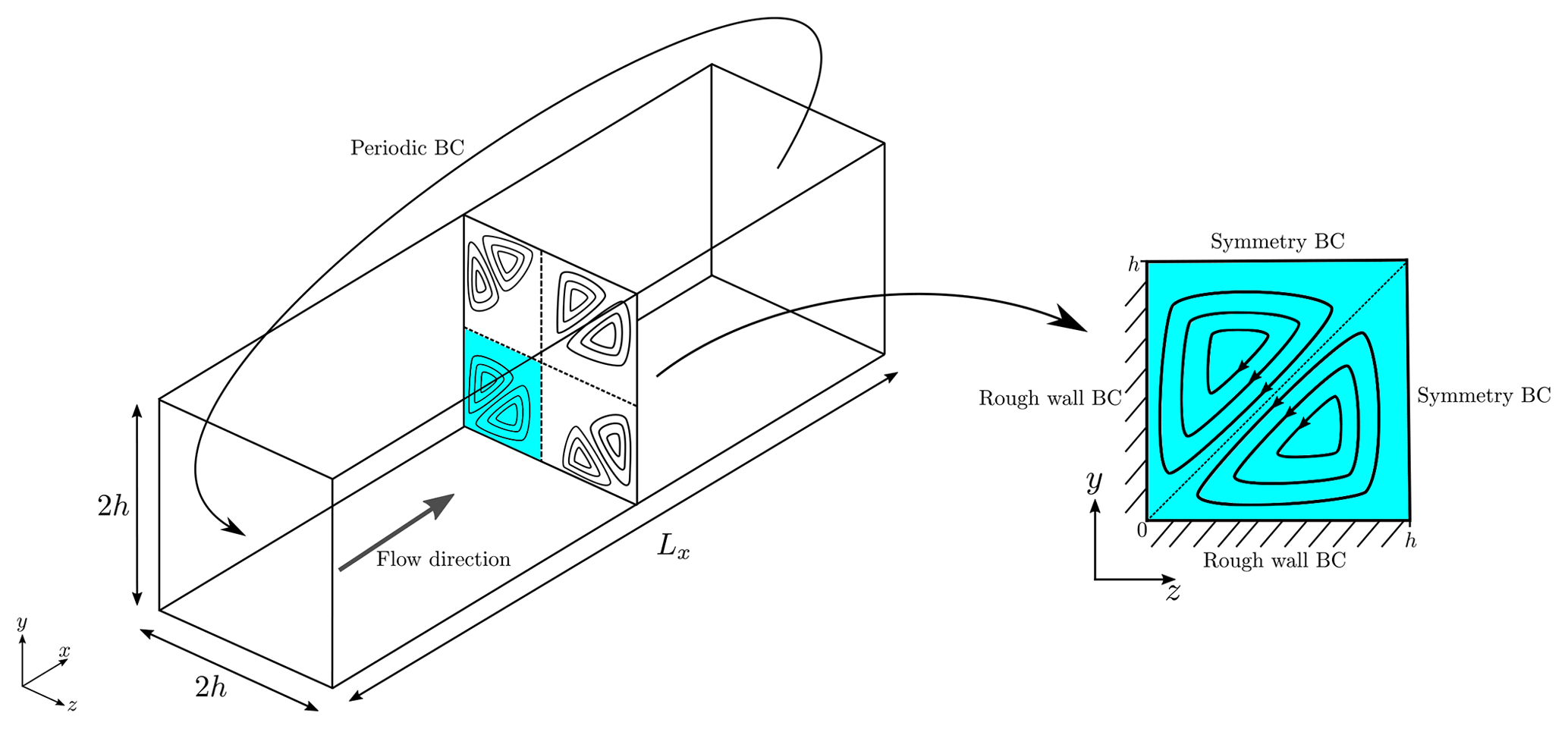
Although, the fully developed square duct flow might appear as a two-dimensional problem, it in fact features a full three-dimensional flow field, due to the secondary corner flows, also sketched in Fig. 7, which were first observed experimentally by Nikuradse (1930) and later with DNS by Gavrilakis (1992). The secondary motions are only on the order of but still have a notable effect on the bulk flow as they transport momentum from the center of the duct toward the corners. Perhaps the most interesting aspect of square duct flow from a turbulence modeling perspective is that linear EVMs are unable to predict the secondary corner flows because the secondary motions are caused by the normal anisotropy components, which are zero in linear EVMs for fully developed flow; see Eq. (5) and discussions by Menter et al. (2009) and Emory et al. (2013). However more sophisticated turbulence models such as EARSM and uncertainty quantification models (Emory et al., 2013) are able to predict this physical phenomenon.
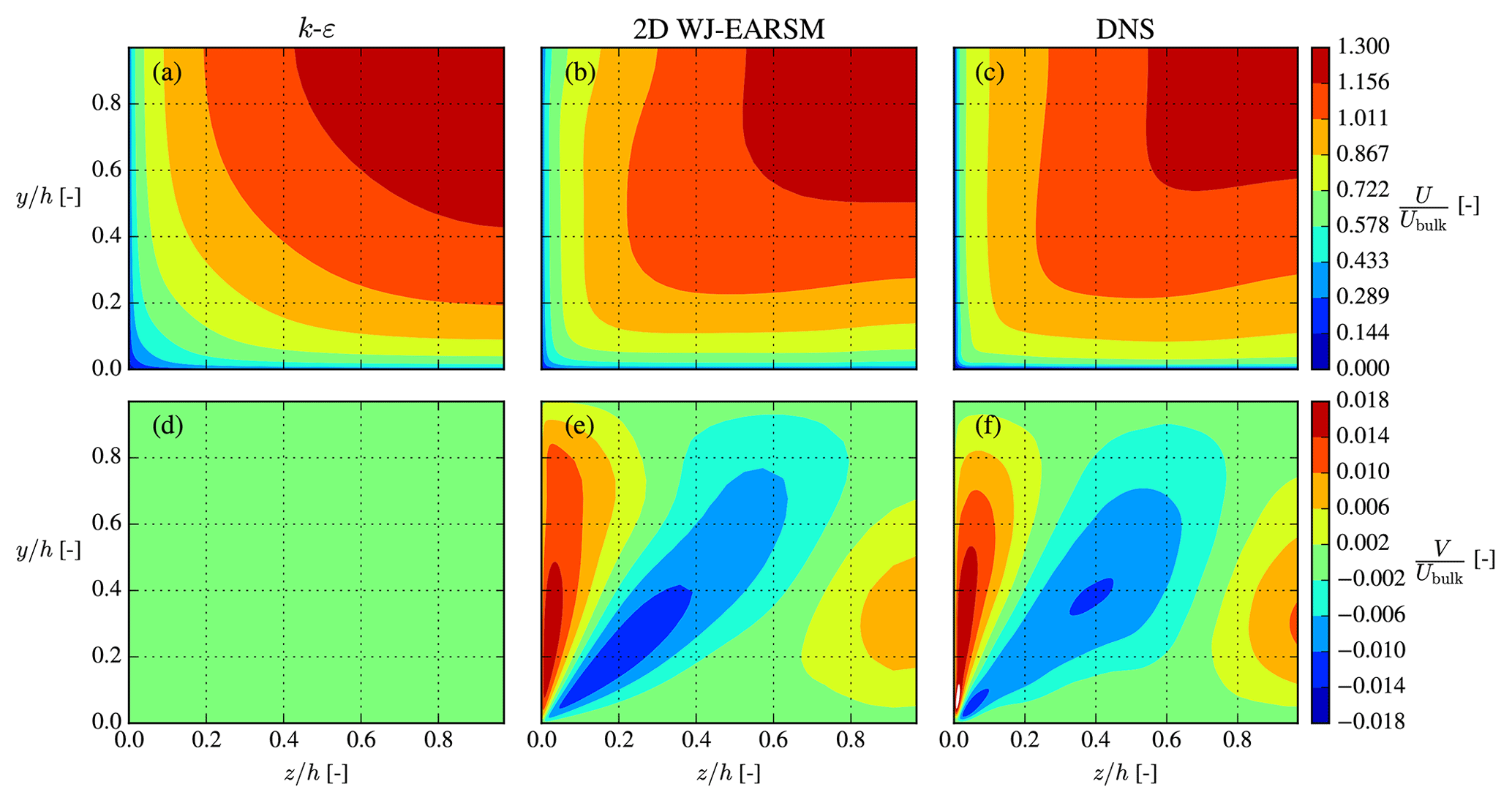
Figure 8Streamwise (a–c) and vertical (d–f) velocity contours in the lower left quadrant of the square duct. Normalized by the bulk velocity, .
In this paper, we simulate a fully turbulent square duct flow (high Reynolds number) with rough-wall BCs; hence the flow is independent of ν similar to the half-channel flow. Currently, the DNS of Pirozzoli et al. (2018) is the most turbulent DNS available (), so this is chosen for reference, although it uses smooth walls and might not correspond exactly to our high-Reynolds-number case. For this reason the RANS and DNS should not be compared directly, but the DNS will at least show typical characteristics and the order of magnitude to be expected. The parameters for the RANS simulation are given in Table 5, and a rectilinear grid is used, which is stretched towards the walls to obtain a first wall-adjacent cell height on the order of the roughness length (no stretching used in streamwise direction).
Table 5Parameters used for simulation of square duct flow in EllipSys3D. The brackets 〈〉 signify the average over the wall.
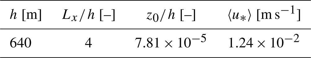
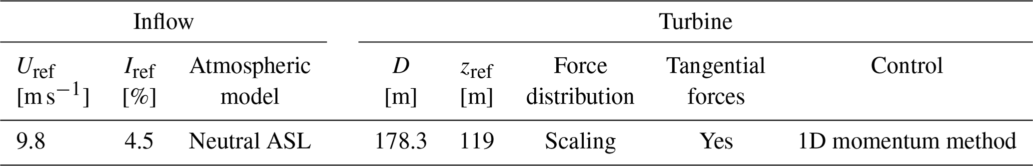
Table 6Simulation parameters for the single-wake V80 case. Note that the LES uses neutral PDBL for the atmospheric model.
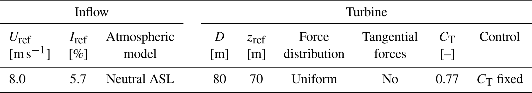
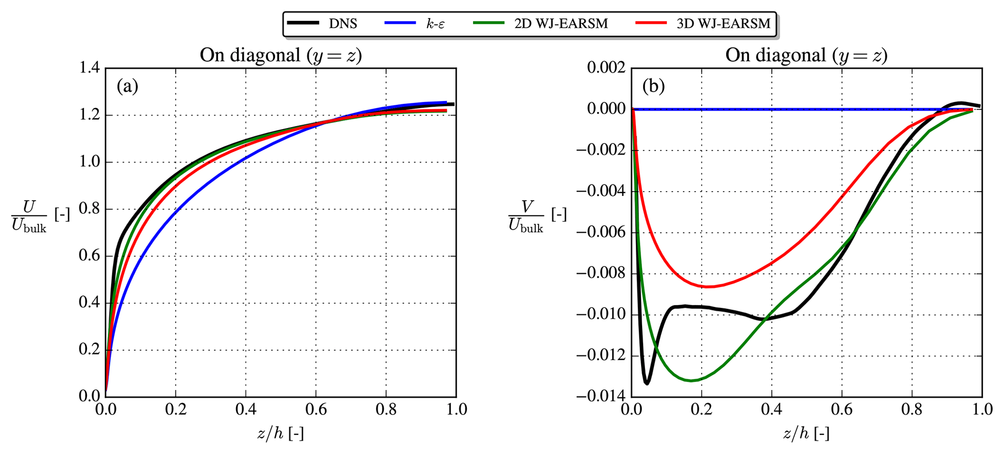
Figure 9Streamwise velocity (a) and vertical velocity (b) on the corner bisector line. Results extracted at .
The streamwise and vertical velocities (U and V components) are shown in Fig. 8, which shows that the 2D WJ-EARSM is indeed capable of predicting secondary flows similar to the DNS of Pirozzoli et al. (2018). Both Figs. 8 and 9 clearly show that the prediction of the secondary flow is necessary to capture the correct shape of the U distribution. In contrast, the standard k–ε model predicts zero vertical velocity and therefore no secondary flow.
The 3D WJ-EARSM performed similarly to the 2D WJ-EARSM, although with a slightly weaker secondary flow, which can be seen in Fig. 9, where the velocity profiles are extracted on the corner bisector line (the diagonal line). Both WJ-EARSMs predict similar profiles to the DNS, although without the near-corner peak, which according to Pirozzoli et al. (2018) is caused by scale separation (this phenomena only occurs at higher Reτ and is thus not visible in the earlier DNSs by Gavrilakis, 1992, and Huser and Biringen, 1993), and this effect is not captured by RANS.
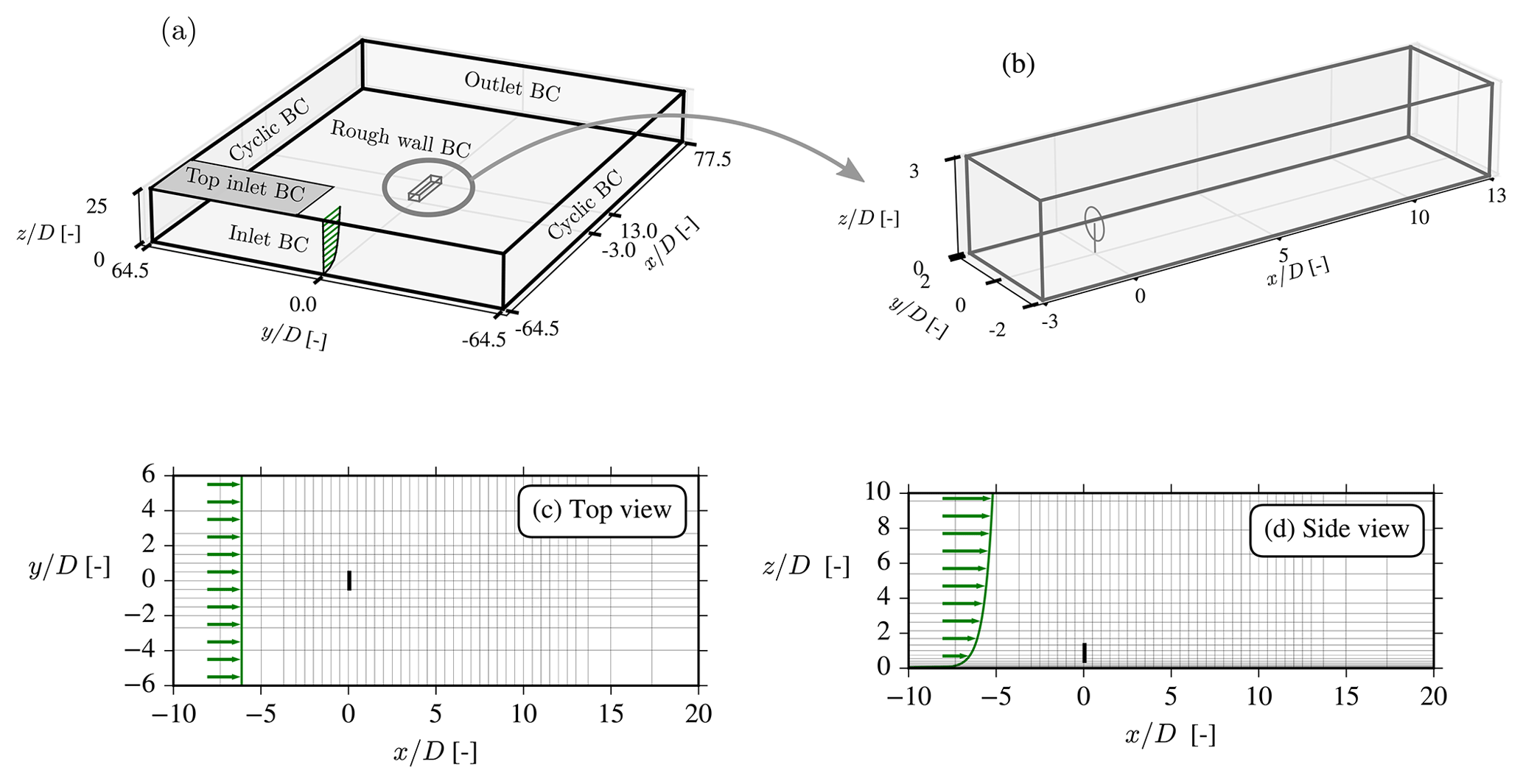
Figure 10Flow domain (a), finely resolved wake domain (b), x–y cut at hub height (c), and x–z cut at centerline (d). Every fourth cell is displayed in panels (c) and (d), and green arrows show velocity profile (not to scale).
This concludes the verification studies, where the WJ-EARSM has been seen to give expected results for three canonical flows. Furthermore, the last case of square duct flow clearly demonstrates that EARS models are able to predict physical phenomena that two-equation models based on the linear Boussinesq hypothesis cannot do.
This section concerns the application of the EARS model to a single-wind-turbine wake. The numerical CFD setup is similar to that used in many previous RANS studies (e.g., van der Laan, 2014; van der Laan et al., 2021; Baungaard et al., 2022): the RANS equations are solved using the SIMPLE method using a modified Rhie–Chow algorithm (Troldborg et al., 2015), while the convective terms are discretized with the QUICK scheme; see more details in Sørensen (1995). To model the wind turbine, an AD with uniform distribution of forces is used (the thrust forces are fixed, and no tangential forces are present), and the forces are transferred to the rectilinear flow domain with the intersectional method of Réthoré et al. (2014). The flow domain has a finely resolved “wake domain” in the center with uniform spacing of , and the grid is stretched outwards in all directions from this using the hyperbolic tangent method of Thompson et al. (1985); see Fig. 10. A grid convergence study was made to confirm that this grid resolution is also suitable for the EARS turbulence model; see Appendix A.
The case simulated is similar to the case used by Hornshøj-Møller et al. (2021), namely a single V80 turbine subject to neutral inflow; see Table 6. The authors of the aforementioned study have provided LES data to us, which are used as a reference in the following. It should be noted that their RANS simulations use ASL inflow (like we shall also use for our RANS simulations), while their LES is based on PDBL inflow. Although there will be differences between ASL and PDBL inflow, the latter is likely a good approximation of the former in the lower part of the domain, but its bias on wake simulations could be a subject for future studies.
4.1 Inflow
The neutral ASL inflow profile (Panofsky and Dutton, 1984) is prescribed at the inlet BC and top of the domain:
This type of inflow is routinely used in wind energy applications, and for a wake simulation it can be adopted to give a desired hub height velocity, Uref, and hub height turbulence intensity (TI), Iref, by adjusting u* and z0 (van der Laan et al., 2015b). One could alternatively adjust Cμ instead of z0 to obtain a desired Iref, but this was shown by van der Laan (2014) to give inconsistent results with the k–ε–fP model and NLEVMs, so this practice is not recommended. Although the adjusted u* and z0 do not correspond to the physical values at the site, it is of higher priority to have the correct Uref (and thereby correct thrust coefficient) and Iref.
In the freestream, the neutral ASL profiles, Eq. (22), should satisfy and to be in balance and mitigate development of the inflow profiles in the streamwise direction. There will inevitably be a slight development (see Blocken et al., 2007), and for this reason a long domain is used to ensure fully developed profiles at the entrance of the wake domain. To satisfy the balance criteria, the turbulence constants should follow the relation (Richards and Hoxey, 1993)
Indeed, both sets of constants in Tables 1 and 2 satisfy Eq. (23).
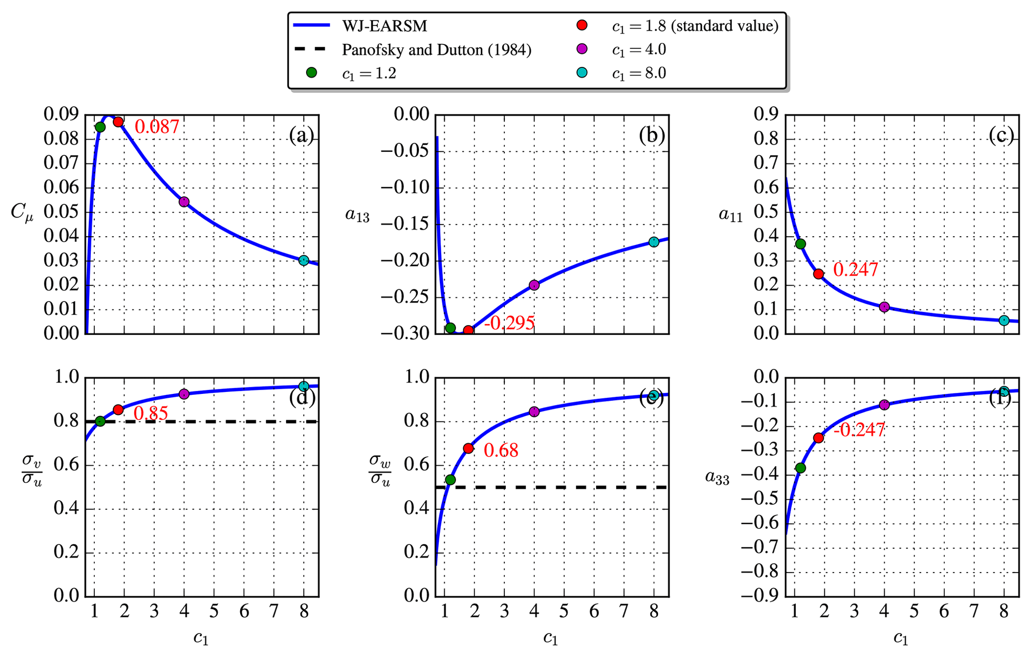
In the neutral ASL, we have , similar to the log layer of the half-channel flow but at all heights. By utilizing the WJ-EARSM the equilibrium relations between the c1 constant and various other variables, as shown in Fig. 11, can be derived analytically. For example, the standard value of c1=1.8, which is used in this paper, gives Cμ=0.087 (the “equilibrium value” mentioned in Sect. 2.3.1). A closer agreement of the velocity standard deviation ratios, and , is seen with the WJ-EARSM, when benchmarking against the ASL ratios of Panofsky and Dutton (1984); the k–ε and k–ε–fP models have , while the WJ-EARSM has and for c1=1.8. In fact, the WJ-EARSM underpredicts the streamwise fluctuations due to the simplification introduced by setting (this is also the case for half-channel flow; see Wallin and Johansson, 2000), resulting in the observed overprediction of the and ratios. Other c1 values (three other choices than the standard value are marked with dots in Fig. 11) will enhance/decrease the ASL anisotropy (see details in Appendix B), but for the present simulations the standard model coefficients of Table 2 are used.
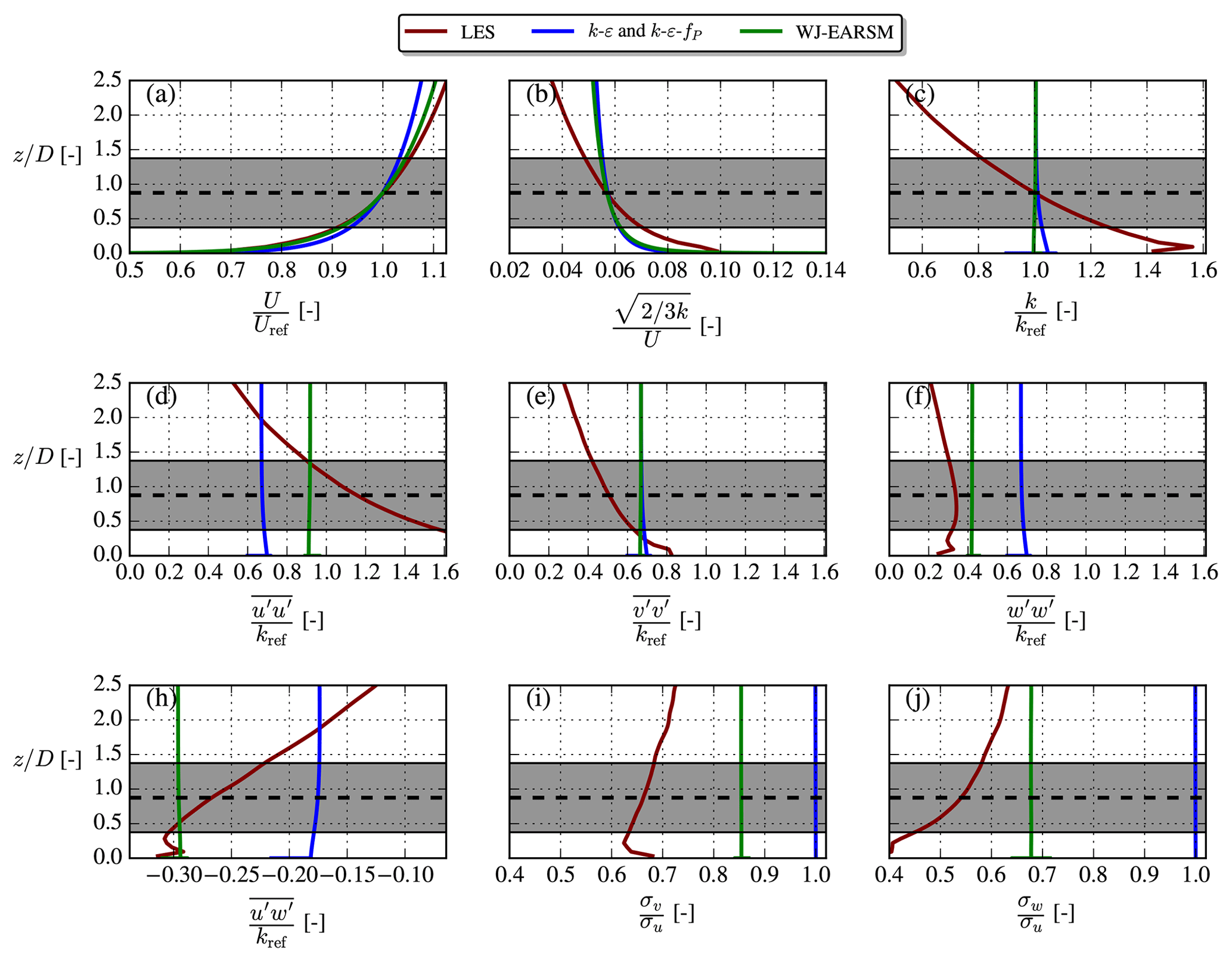
The inflow profiles of the LES and RANS simulations are shown in Fig. 12. Since the k–ε and k–ε–fP models are identical in the freestream, which is also true for the 2D and 3D WJ-EARSMs, only one of the other is shown in the figure. The LES is driven with a streamwise pressure gradient and thus differs in the stress profiles compared to the pure ASL profiles used in our RANS, but Uref and Iref do match. As in the half-channel case, the velocity shear differs due to the different κ and Cμ used in the k–ε–fP model and WJ-EARSM, and the stress profiles are also different between the two because of the anisotropic nature of WJ-EARSM. In terms of turbulence anisotropy, quantified as the distribution of TKE between the normal stress components in Fig. 12, the WJ-EARSM is clearly closer to the LES data as was also expected from the analytical results in Fig. 11.
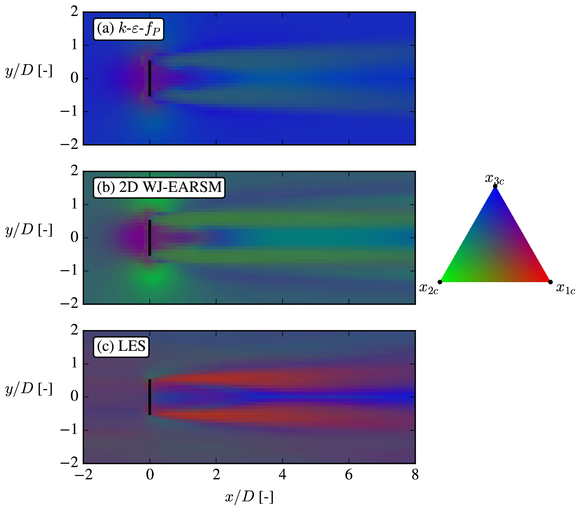
Eigendecomposition of the Reynolds stress tensors can be used to describe the turbulence state through its three real eigenvalues, which describe the fluctuations in the three orthogonal, principal directions. Several techniques (e.g., eigenvalue map, invariant map, barycentric map, and Lumley triangle) combine the eigenvalues and visualize them with two-dimensional maps; in Fig. 13 the barycentric map is used with the RGB color scheme of Emory and Iaccarino (2014). Both RANS models use ASL inflow; hence the turbulence state is the same at all heights, whereas the LES state varies with height due to its PDBL inflow. The k–ε–fP turbulence is mostly isotropic (the x3c corner) as is expected for all Boussinesq-type models because normal stresses are , whereas the WJ-EARSM turbulence is perturbed more towards 2D turbulence (the line connecting x2c and x1c) and thereby closer to LES turbulence.
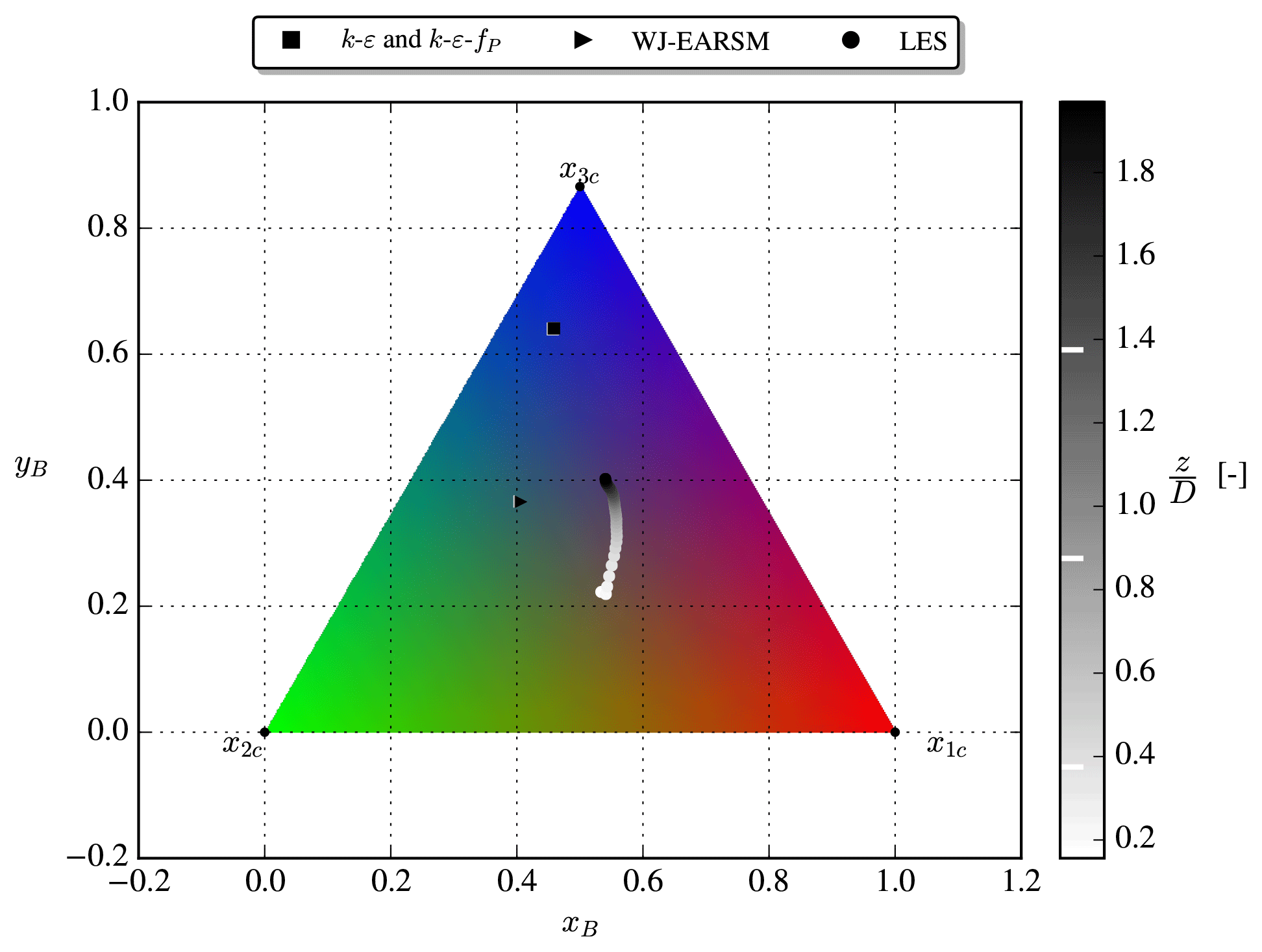
Figure 13RGB-colored barycentric triangle, with RANS/LES inflow data shaded by height; white lines at right mark (zref−R), zref, and (zref+R), respectively.
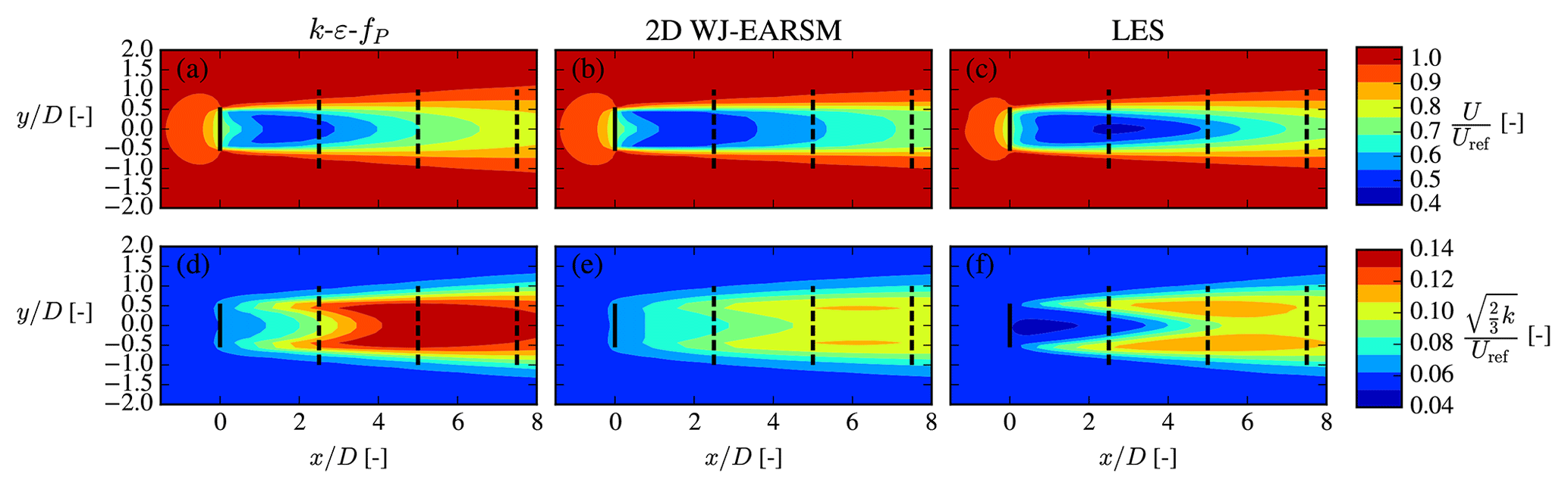
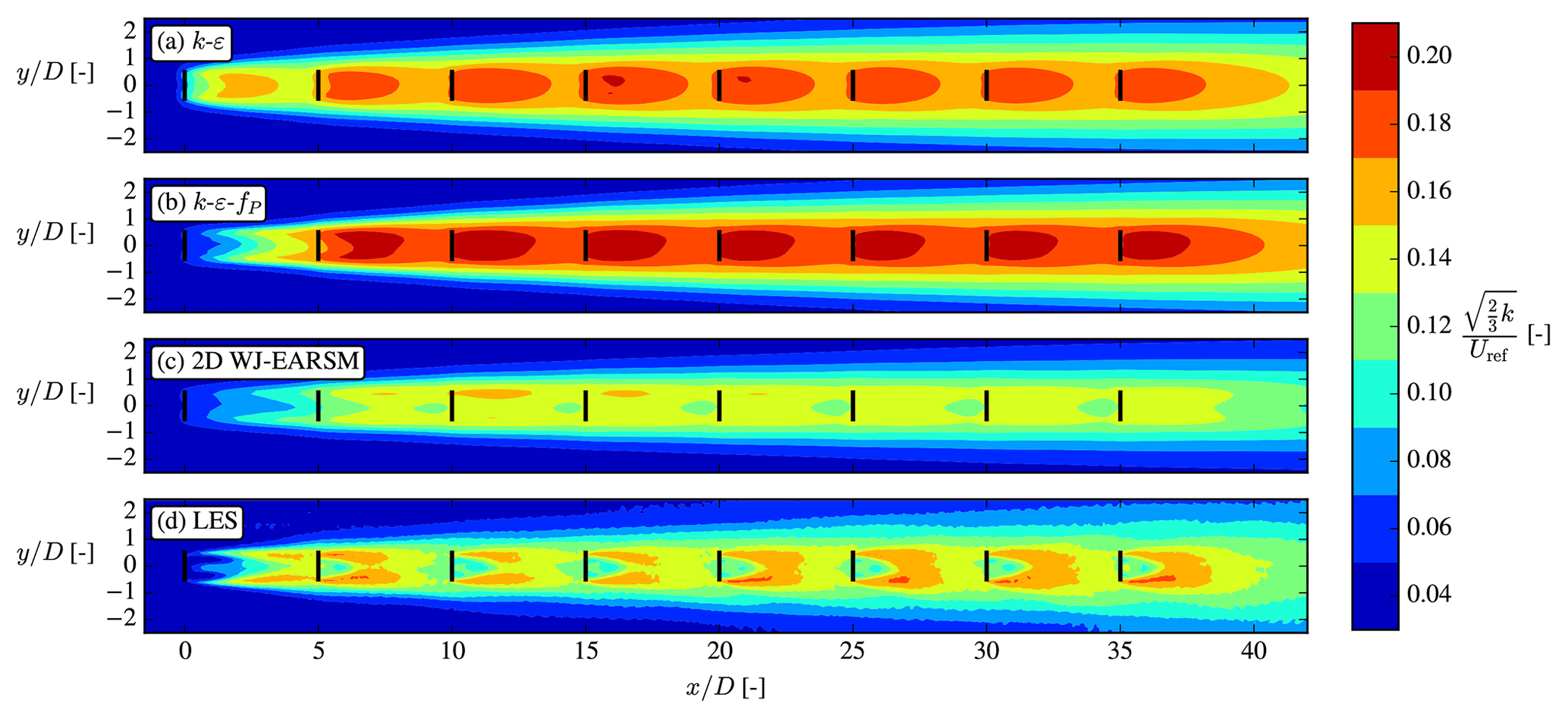
Figure 14Streamwise velocity (a–c) and TI (d–f) contours at hub height for the single-wake V80 case. Full lines mark ADs, while dashed lines mark where wake profiles are extracted.
4.2 Velocity and turbulence intensity
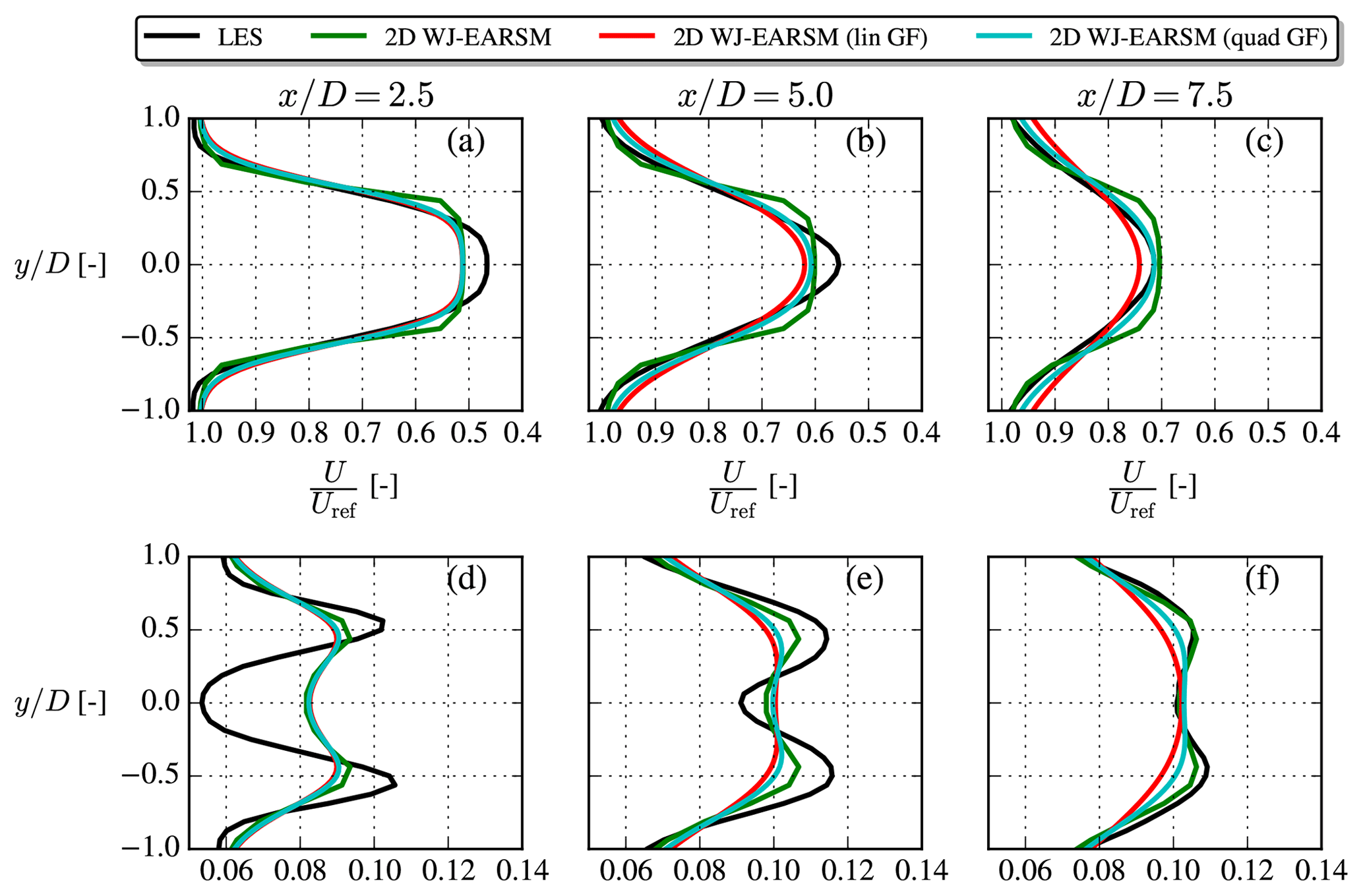
Wake data in the form of velocity and TI contours at hub height and profiles at three downstream positions are shown in Figs. 14 and 15. In addition to the 2D WJ-EARSM, results using the 3D WJ-EARSM with/without tangential AD forces are also shown in Fig. 15, and the first conclusion to draw from this is that the 2D and 3D versions of the WJ-EARSM give similar wake profiles, and we therefore focus on the simpler 2D WJ-EARSM in the following. A simple diffusion correction to the WJ-EARSM was suggested by Wallin and Johansson (2000) to correct the model in regions with low normalized velocity gradients (e.g., at the top of the half-channel), but it only has a small effect on velocity deficit and TI, as seen in Fig. 15, so it is not considered in the following discussions. Finally, results of the standard k–ε model are also shown in Fig. 15 to show its overly diffusive behavior.
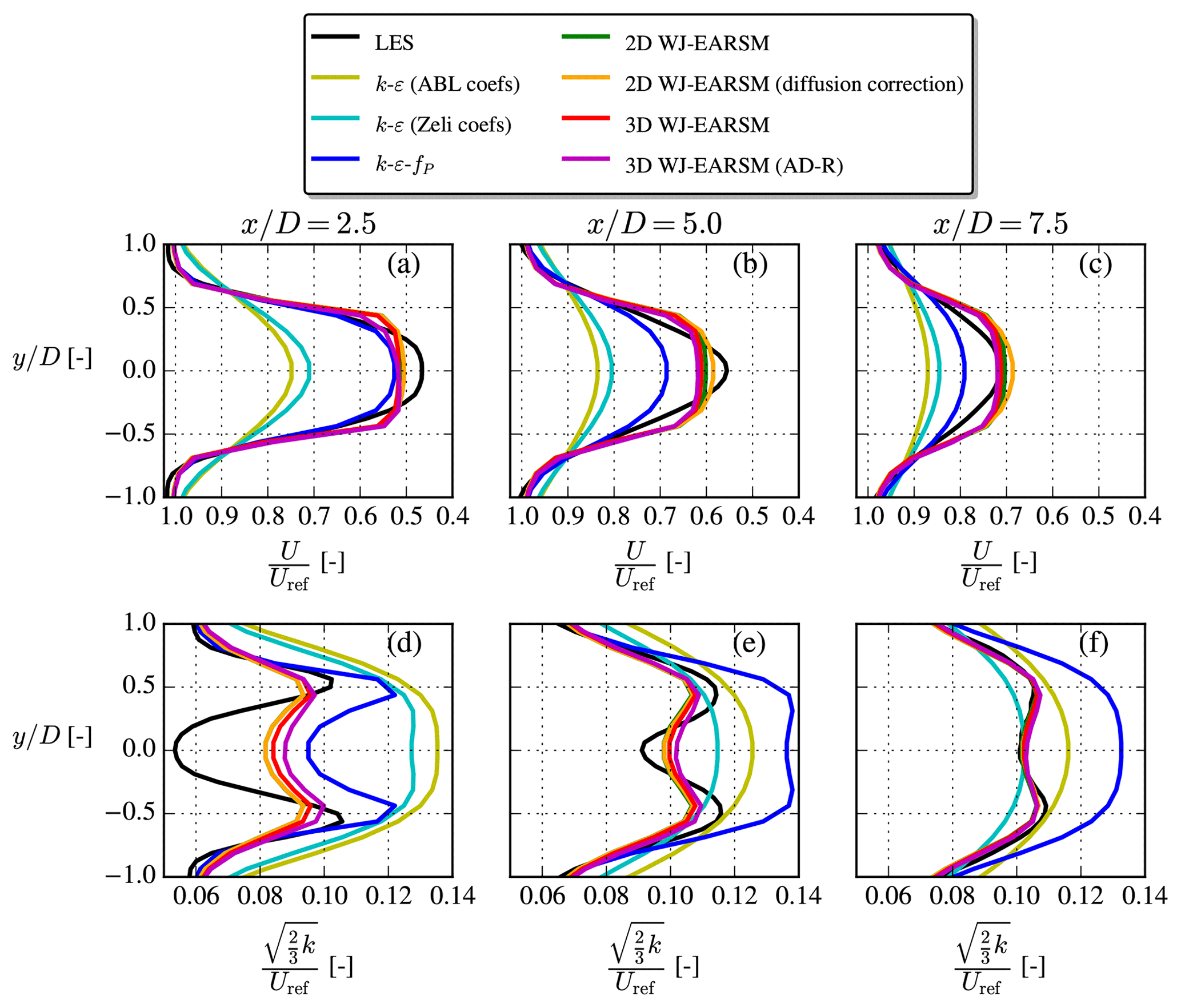
Figure 15Streamwise velocity (a–c) and TI (d–f) profiles extracted at various downstream positions for the single-wake V80 case.
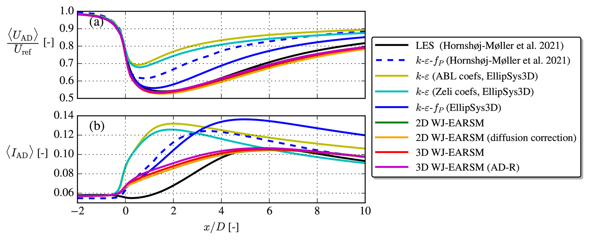
Overall the wake velocity contours in Fig. 14 appear similar, while the TI contours of the WJ-EARSM are improved over the k–ε–fP model; however, similar to the k–ε–fP model, it still fails to predict the TI delay in the near wake seen in the LES, which is also clearly visible in the disk-averaged TI recovery profiles in Fig. 16b. Also, there is a TI induction zone in both RANS simulations, which is not present in the LES; these two effects seem to be a general issue of k–ε-based RANS models as this was also observed with the standard k–ε, realizable k–ε, and re-normalization group (RNG) k–ε models by Hornshøj-Møller et al. (2021).
Considering the wake profiles in Fig. 15, it is clear that WJ-EARSM produces more “top-hat-shaped” profiles similar to the classic Jensen model (Jensen, 1983). This has also been seen with other EARSMs (van der Laan, 2014) and with full differential RSMs (Cabezón et al., 2011; Tian et al., 2019). One can either apply the previously mentioned diffusion correction or increase the c1 constant to obtain a more Gaussian-shaped profile for the WJ-EARSM, but the latter is not recommended as it will deteriorate the ASL anisotropy; see Appendix B. Another view is that the top-hat-shaped profile is a consequence of not taking various physical phenomena into account, e.g., large-scale atmospheric turbulence and wake instabilities, and applying a unidirectional wind direction in our idealized RANS setup (in the transient LES there will be a varying instantaneous wind direction throughout the simulation). These types of effects could be interpreted as a Gaussian filter on the wake profiles; see discussion in Appendix C. Note that the k–ε–fP model already accounts for at least the wind direction effect as it has been calibrated with LES, which includes a wind direction distribution (van der Laan, 2014), and that it could be recalibrated to obtain a better match with the velocity deficit of the present LES case (since the latter LES was simulated with a different solver and AD implementation).
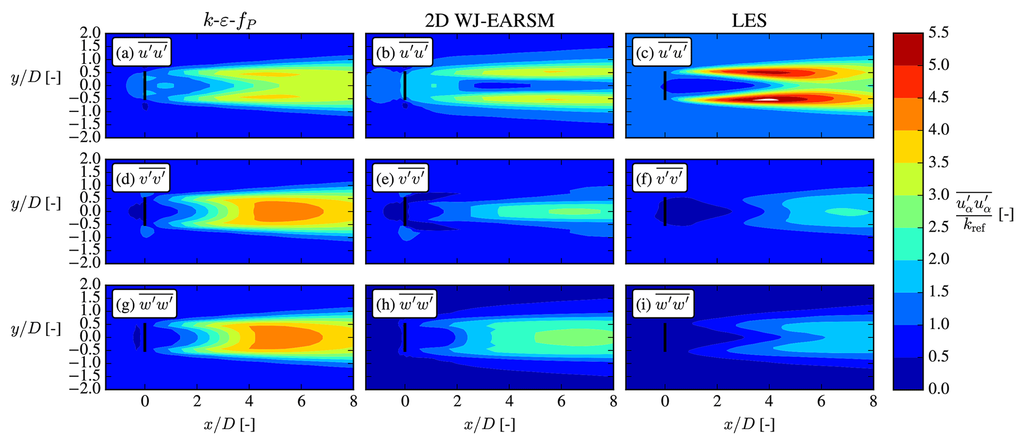
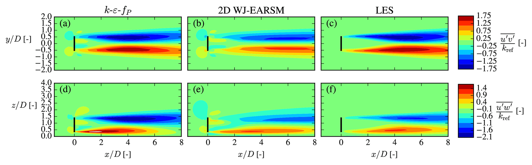
Figure 18Lateral U momentum flux at hub height x–y plane (a–c) and vertical U momentum flux at the center x–z plane (d–f) for the single-wake V80 case.
Lastly, we want to emphasize that the turbulence model is not solely responsible for the wake results: the same turbulence model applied for the same case but with different codes/solvers can yield significantly different results, as can be seen in the comparison of the k–ε–fP results in Fig. 16. This reminds us to be careful with general conclusions on which is the better turbulence model.
4.3 Stresses
For more insights on the wake mixing and turbulence, we now turn to the second-order statistics of turbulence, namely the individual Reynolds stress components. The normal components are shown in Fig. 17, which shows that the WJ-EARSM correctly dampens the lateral and vertical components, which are otherwise overestimated severely by the k–ε–fP model due to its Boussinesq closure. This also explains the lower TI of the WJ-EARSM in Fig. 14–16 as the TI is composed of the sum of the normal components. On the other hand, the normal stress contours seem too elongated in the streamwise direction with the WJ-EARSM; for example the low core in the center of the wake in Fig. 17b extends too far downstream compared to the LES data in Fig. 17c, which is possibly connected with the decreased turbulence mixing also causing the top-hat profiles of wake deficit shown in Fig. 15. Increasing the c1 constant will alleviate this specific issue; see Appendix B.
Transport of U momentum by turbulence, , from the ambient high-speed surroundings to the low-speed wake region is mainly determined by the off-diagonal components of the Reynolds stress tensor, and , i.e., the lateral and vertical turbulent fluxes of U, respectively, which are shown as contours in Fig. 18. Both are larger in absolute magnitude for the k–ε–fP model compared to WJ-EARSM, leading to larger gradients of the stresses and explaining the increased wake recovery of the former, but when comparing to the LES data, it can be noticed that the magnitude of is overestimated, hence the overestimated wake recovery of the k–ε–fP model in Fig. 16. On the other hand, the WJ-EARSM underestimates the magnitude of the fluxes, especially notable in the contours, hence the slight underestimation of wake recovery compared to LES in Fig. 16.
Table 7Simulation parameters for the aligned-row case from TotalControl. The AD scaling and 1D mom'm control methods are described in detail by van der Laan et al. (2015a).
To conclude, we see some advantages but also disadvantages with using WJ-EARSM over the k–ε–fP model for prediction of the Reynolds stresses, which also has direct consequences for the prediction of the velocity deficit and turbulence intensity.
4.4 Turbulence state
In the inflow section, Sect. 4.1, it is shown that the turbulence state of the freestream turbulence was mainly isotropic in the k–ε–fP model, while both the WJ-EARSM and LES data were more perturbed towards 2D turbulence (the lower edge in the barycentric triangle). This is also seen in the RGB-colored x–y plane at hub height in Fig. 19, where one can see that the ambient flow of the k–ε–fP model is predominantly colored blue and is hence isotropic. As also alluded to in Sect. 4.1, the ambient WJ-EARSM turbulence is more oblate (left edge of barycentric triangle), while the LES is more prolate (right edge of barycentric triangle), hence the green and purple coloring, respectively, of the ambient flow in Fig. 19. In the wake shear layers, both RANS models predict perturbations towards 2D turbulence, while LES is more perturbed towards 1D turbulence (the x1c corner). These observations fit with the increase in and strong damping of and in the LES shown in Fig. 17. To improve the prediction of the turbulence state, we therefore suspect that normal stress predictions are essential, especially the ratios of those – the WJ-EARSM definitely has some improvement from the overly isotropic k–ε–fP model but does not capture the completely right ratio between normal stresses. We note that a resolution of 20 cells per diameter was used in the reference LES, which might be sufficient for first-order statistics and shear stresses but could bias the normal stresses and therefore also the turbulence state.
To test the WJ-EARSM in a wind farm scenario, we simulate the lower row in the TotalControl rot90 reference wind farm, which consists of eight aligned wind turbines with 5 D inter-spacing; see Fig. 20. The DTU 10 MW turbines of the wind farm are modeled with the scaling AD method with 1D momentum control (van der Laan et al., 2015a) and including tangential forces (hence there will be wake swirl), and the thrust, rotational speed, and power curves are taken from the DTU 10 MW report (Bak et al., 2013). We compare the results with LES conducted at KU Leuven (the “PDk90 case”; Sood and Meyers, 2020), where the turbines were modeled with an actuator surface (AS) model coupled to an aeroelastic code; hence the LES and RANS are not directly comparable but nevertheless give a reference to compare against. Due to the natural streaks appearing in LES, we choose to calculate Uref and Iref with planar averages of the LES data in the region upstream of the lower row rather than using the time-averaged precursor profiles. The overview of the simulation parameters is given in Table 7. The numerical setup of the RANS simulation is identical to the one used for the single-wake case, except that tangential forces and non-uniform thrust forces are applied on the AD, the domain is scaled with the new rotor diameter, and the wake region is extended to encompass all eight turbines.
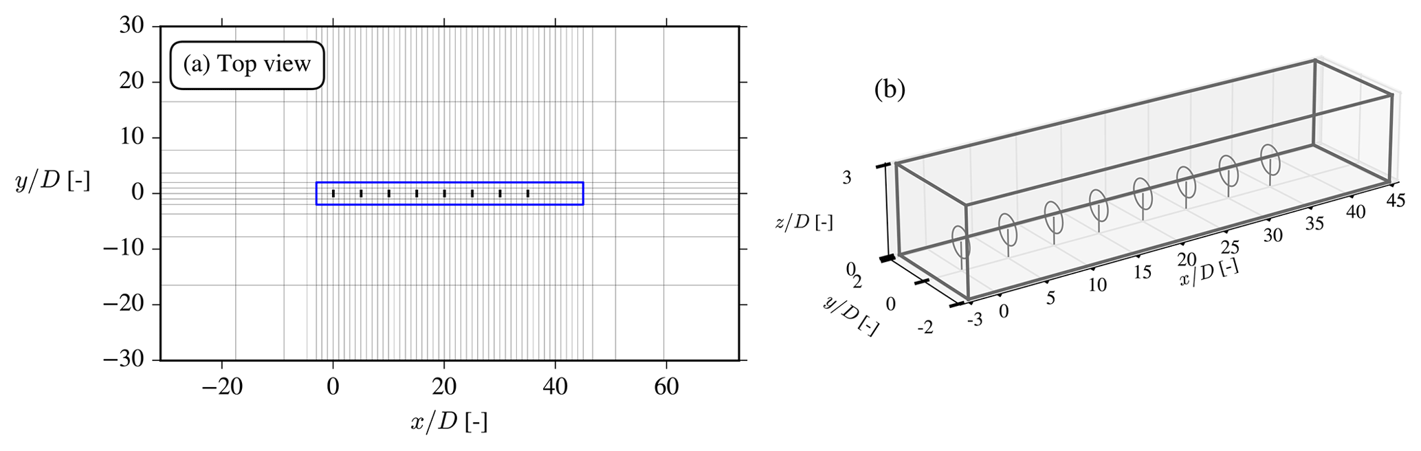
Figure 20A x–y cut of the domain with every eighth cell shown (a) and a 3D view of the wake domain (b) for the aligned-row case. The size of the domain is , , and . A rough-wall BC and an inlet BC are used for the lower and upper BCs, respectively.
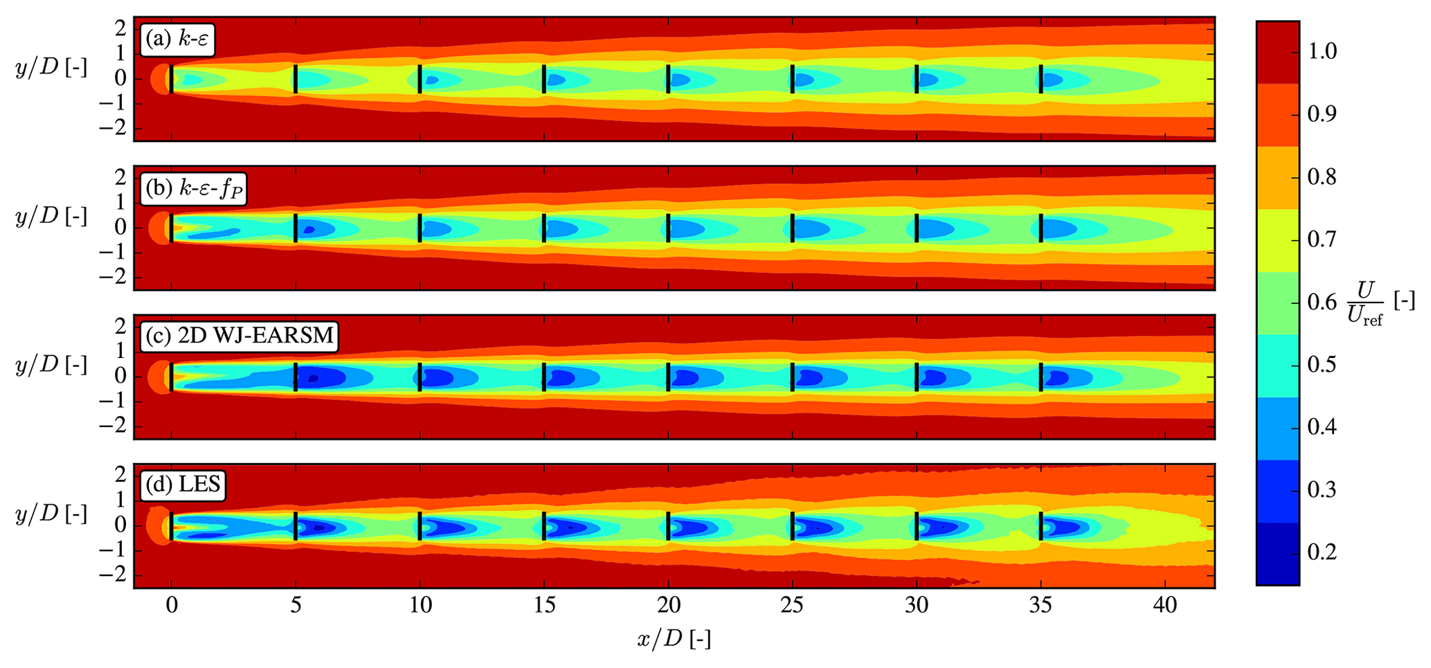
The velocity contours in Fig. 21 show that both the k–ε–fP model and WJ-EARSM qualitatively share some of the same flow features as the LES; e.g., a faster wake recovery is seen on the left side of the first wake (seen from upstream) because of the combined effect of wind shear and wake rotation (a.k.a. swirl), and they predict the largest wake deficit in the second wake. Neither of these effects are predicted by the standard k–ε model, but it can capture other phenomena as for example the induction zones and the expanding wake tube surrounding the whole row. Figure 23a shows the streamwise velocity along the axial line of the ADs and shows that the WJ-EARSM is closer to the LES in the near wake of each turbine, while the k–ε and k–ε–fP models are better at the far wake of each turbine. The RANS models become more similar further down in the row, and the recovery behind the last turbine (a.k.a. the wind farm recovery) is very similar. In van der Laan et al. (2015c), a similar observation was made when comparing the standard k–ε and k–ε–fP models for wind farm cases since the difference between both turbulence models reduces with increased levels of turbulence.
The turbulence intensity contours in Fig. 22 show more pronounced differences between the models; e.g., the LES has peaks of TI in the wake shear layers, whereas the RANS models have TI more evenly distributed over the wake. As is also seen and discussed in the V80 case, there is no induction zone of TI for the LES, and the development of TI is delayed. Again also the WJ-EARSM has lower TI compared to the k–ε and k–ε–fP models and is in better agreement with the LES.
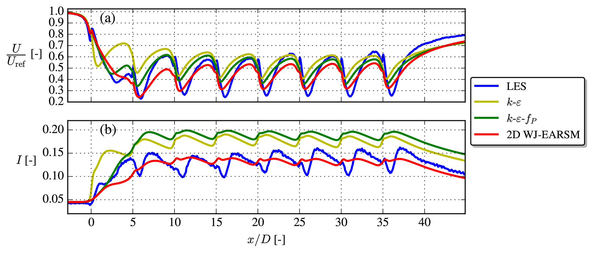
Figure 23Streamwise velocity and turbulence intensity at the axial line going through the AD centers for the aligned-row TotalControl case.
In conclusion, the WJ-EARSM appears numerically stable and well behaved (e.g., no monotonic decreasing velocity deficit or other unphysical effects) for interacting wakes, and as in the single-wake case, there are both some improvements and some less desirable effects of the model over the k–ε–fP model.
This paper documents and explains our implementation and application of an EARSM (Wallin and Johansson, 2000) as a turbulence model for RANS simulations of wind turbine wakes, in the neutral ASL. To our knowledge, EARSM is rarely – if ever – used in the wind energy community; but we show that it is actually relatively straightforward to implement in CFD codes that already employ two-equation turbulence models and importantly that the WJ-EARSM also appears to be numerically stable for wake simulations. Previous attempts by van der Laan (2014) of applying EARSMs (models of Taulbee, 1992; Gatski and Speziale, 1993; and Apsley and Leschziner, 1998) for wake simulations showed problems with numerical stability, even for single-wake cases, but this appears to not be an issue for the EARSM of Wallin and Johansson (2000). The reason for the better numerical behavior most likely lies in the self-consistent formulation of particular importance in regions with rapid shear, hence preserving physical realizability.
Three canonical flow cases – homogeneous shear flow, half-channel flow, and square duct flow – were used to verify the implementation of the model and also showcased some of the advantages with an EARSM over traditional linear EVMs, namely the prediction of freestream turbulence anisotropy and secondary flow phenomena. All three cases have either analytical asymptotes or DNS data to compare against and are easy to set up, which makes them ideal for verification purposes.
For neutral ASL inflow we show that there is a delicate relationship between the turbulence constants that needs to be fulfilled to ensure a non-developing freestream solution and that it also dictates the amount of freestream turbulence anisotropy. It should be noted that this balance of constants is also important for numerical robustness. Comparing the RANS inflow with reference LES data shows that the WJ-EARSM is capable of predicting similar freestream anisotropy, whereas the turbulence of the k–ε–fP model is nearly isotropic (although not exactly) by definition of its Boussinesq closure. This is also clear from the eigendecomposition of the Reynolds stress tensor, which was visualized with the barycentric map technique.
A single-wake case was considered first, and it was observed that the 2D version of the EARSM yielded almost identical results to the 3D version, even when tangential forces were applied on the AD; thus we use the 2D model for the remainder of the paper. It should be noted that the 2D version of the WJ-EARSM is a complete and invariant model for general three-dimensional mean flows. Only the particular dependency of pure three-dimensional effects is simplified, which will have a minor impact on most three-dimensional mean flows of interest. The wake profiles of the EARSM were more top-hat-shaped than the profiles observed in the LES data, which might be related to the underlying weak-equilibrium assumption and limitations in the length-scale-determining ε model equation but could also be caused by wind direction variations (see Appendix C). The disk-averaged velocity deficit and turbulence intensity recovery profiles were however improved over the k–ε–fP model for the specific case considered. It is also possible to obtain a more Gaussian-shaped wake profile by increasing the c1 constant and re-tuning the turbulence model constants, but this will deteriorate the prediction of the underlying ASL anisotropy (Appendix B). A notable difference between the WJ-EARSM and the k–ε–fP model is also that the latter predicts large peaks of lateral and vertical normal Reynolds stress components in the wake, which are not present in the LES data, because of the Boussinesq closure; this deficiency and the low value of Cμ used for the k–ε–fP model are possibly the reasons why it tends to overpredict turbulence intensity in the wake.
Finally, we simulated a row of eight aligned turbines, where the trends from the single-wake case could also be seen, e.g., the top-hat-shaped profiles and better turbulence intensity prediction with EARSM. There were more uncertainties in the comparison with the LES data in this case because different turbine modeling techniques were used, but the case nevertheless shows that the EARSM also behaves sensibly in cases with wake–wake interaction in the sense that the code still converges and that no unphysical trends (such as monotonic increase in wake deficit throughout the row of turbines) are observed.
In conclusion, the EARSM of Wallin and Johansson (2000) can be used for wake simulations in a numerically robust way and only has a small computational overhead compared to standard two-equation models (on the order of 5 % for the V80 single-wake case); hence it is at least 3 orders of magnitude faster than LES. It provides an advantage over two-equation models in the sense that it has more realistic inflow with anisotropic turbulence and that the wake turbulence also becomes more anisotropic, which indeed is also observed in LES. The turbulence intensity prediction was improved for both test cases considered, while velocity deficit was only considerably improved for the single-wake case; more cases (both LES and experimental data) are needed to draw general conclusions about its performance in this regard.
Atmospheric conditions in thermally stable stratification and thermal convection strongly influence the turbulence states, anisotropies, and in particular the vertical mixing in the ASL. This will have a fundamental influence on the wake development and the performance of wind parks. The extension of the EARSM to non-neutral conditions has over recent years been developed by Lazeroms et al. (2013), and Želi et al. (2019) have subsequently demonstrated the model's capability of capturing these effects. This will be of interest for future wind turbine wake studies.
Earlier studies (van der Laan et al., 2015b) have shown that a grid spacing of in the wake region is sufficient for grid convergence of wake velocity deficits with the k–ε–fP model, and the same conclusion can be drawn for the 2D WJ-EARSM; see Fig. A1. We also plot the TI profiles in Fig. A1, which are more sensitive to grid resolution, but we nevertheless decide to use in this paper because it represents the typical resolution used in wind farm studies and saves a considerable amount of computational resources.
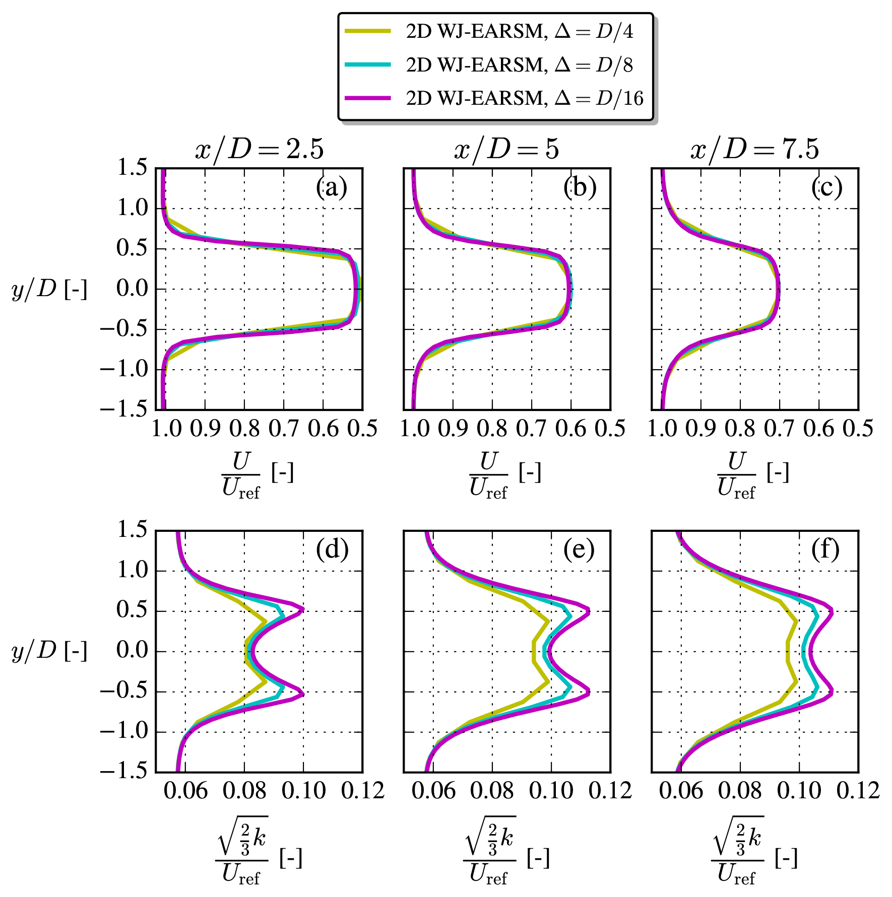
Figure A1Grid study of streamwise velocity (upper row) and TI (lower row) profiles at hub height for the V80 case with the 2D WJ-EARSM using different mesh resolutions.
The c1 constant, a.k.a. Rotta coefficient, in the WJ-EARSM originates from the pressure-redistribution term and can in principle be re-tuned; e.g., the original LRR (Launder–Reece–Rodi; Launder et al., 1975) model has c1=1.5, and van der Laan (2014) used c1=4.5 for the fP model. As shown in Sect. 4.1, for the neutral ASL the WJ-EARSM can be used to obtain a direct relationship between c1 and many other variables in equilibrium; see Fig. 11. From this it is clear that the ASL anisotropy is enhanced for decreasing c1 and vice versa. It is important to emphasize that the variables in Fig. 11 are only dependent on c1 and not the other turbulence constants. In this section we test three different c1 values in addition to the standard value of c1=1.8; see Table B1.
Table B1Tested sets of turbulence model constants and derived variables for the single-wake V80 case. For all sets, we use Cε2=1.82, σk=1.0, σε=1.3, κ=0.38, and .
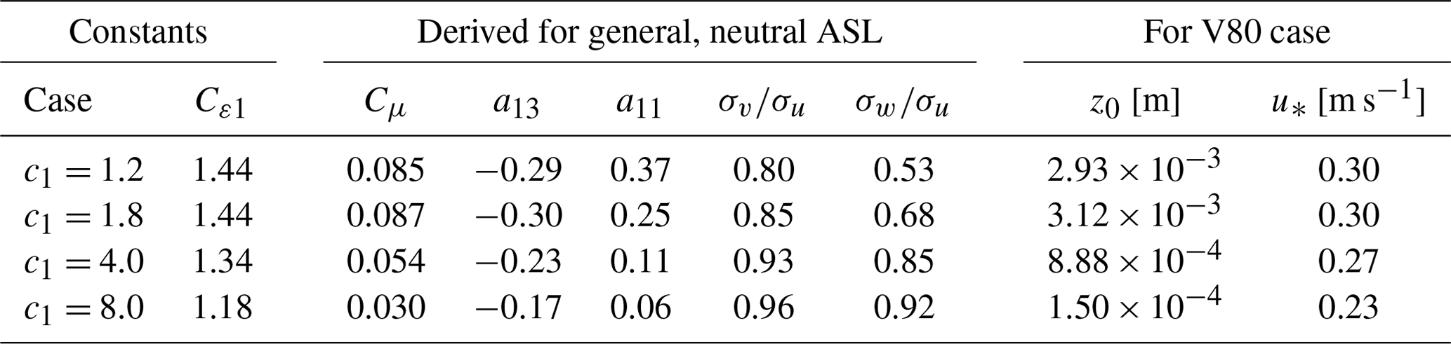
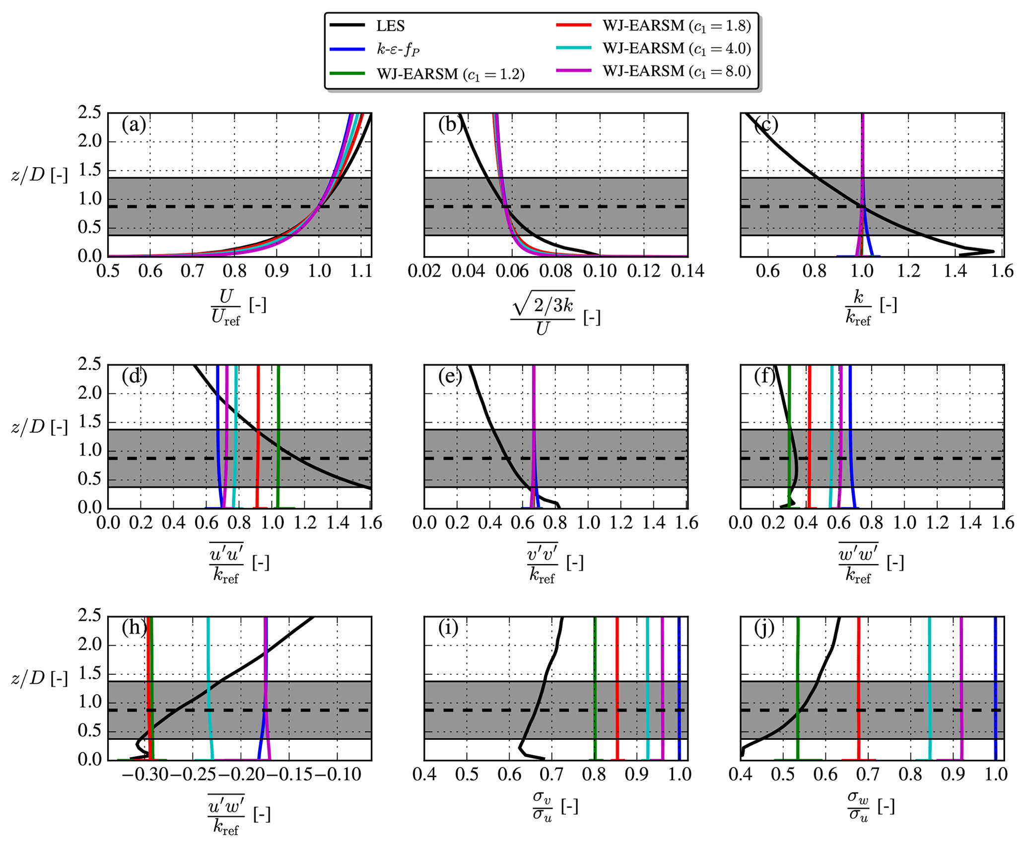
Figure B1Inflow profiles for the single-wake V80 case with different sets of model constants.
Equation (23) needs to be satisfied to have a balanced RANS solution; hence when c1 is adjusted, and Cμ thereby changes, then either κ, σε, Cε1, Cε2, or a combination of all needs to be adjusted. We choose to adjust Cε1 and fix the others, and the resulting sets of constants are shown in Table B1. The first set (c1=1.2) gives anisotropic freestream turbulence close to the Panofsky and Dutton (1984) neutral ASL values; the second set (c1=1.8) is equivalent to the standard set (see Table 2); the third set (c1=4.0) gives Cμ=0.054, which is close to the value used by WAsP CFD (Bechmann, 2016); and finally the last set (c1=8.0) gives Cμ=0.03, which is often used for atmospheric applications (Sørensen, 1995; Richards and Hoxey, 1993).
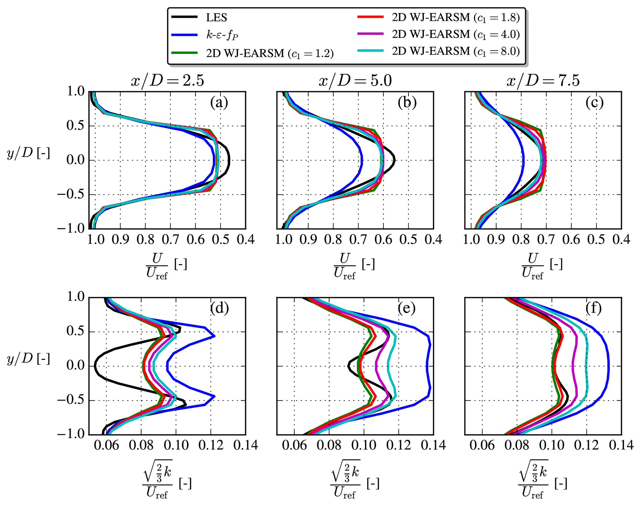
Figure B2Streamwise velocity (a–c) and TI (d–f) profiles extracted at various downstream positions for the single-wake V80 case with different sets of model constants.
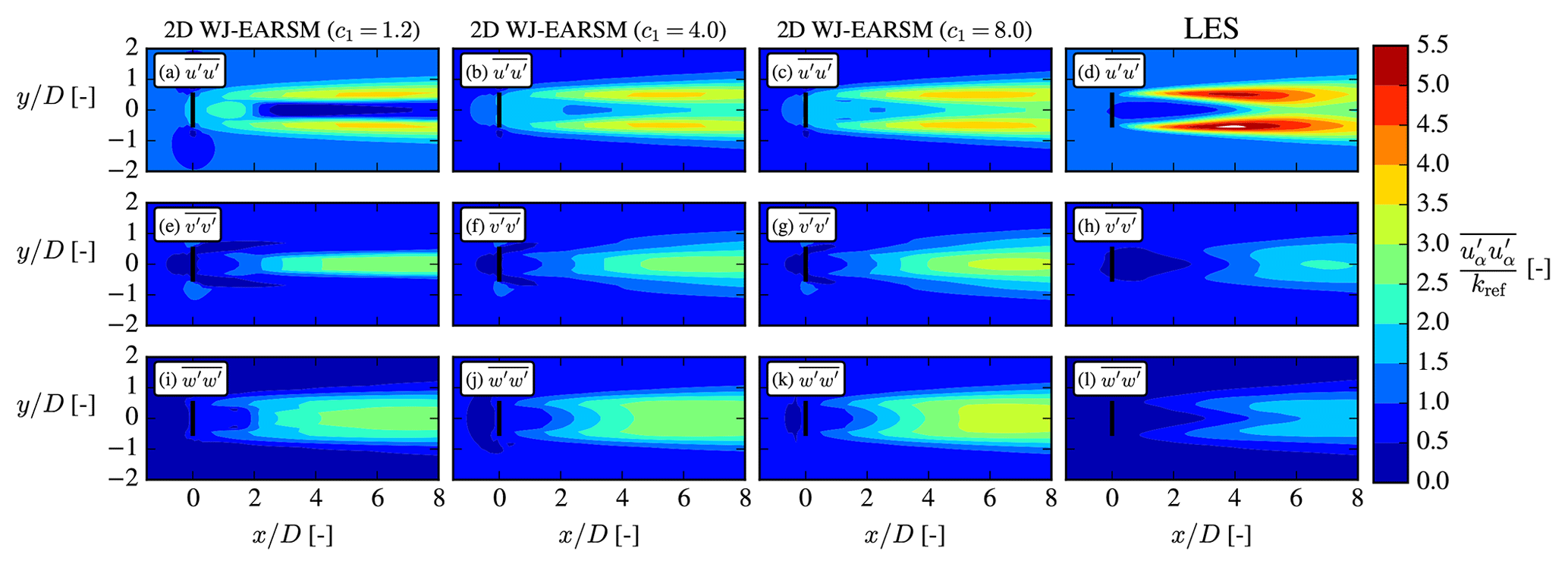
Figure B3Normal stresses at hub height for the single-wake V80 case with different sets of model constants.
Another consideration is that the roughness length and friction velocity also need to be modified to give the same hub height velocity and turbulence intensity according to Eq. (22), again because Cμ changes with changing c1. The values of these are therefore also included in Table B1 and explain why the velocity inflow profiles differ slightly in Fig. B1. The figure also clearly demonstrates that freestream turbulence anisotropy decreases for increasing c1 and vice versa, which is also evident from the combination of Eqs. (10)–(11):
In the derivation of Eq. (B1) we use the definition of N and as well as in the neutral ASL. From Eq. (B1), we see that for increasing c1 there is a decreasing (see Eq. 9), which is the part of the closure responsible for anisotropy and therefore explains why the turbulence becomes more isotropic with increasing c1.
Figure B2 shows how the wake is effected by the new sets of constants. The velocity deficit shape is more Gaussian for larger c1 and thus more similar to the LES shape, while the turbulence intensity increases. From these observations, one could argue that c1=4.0 would perhaps be a better choice for modeling of velocity deficit, while c1=1.8 is better for TI and anisotropy predictions.
Increasing c1 also has a significant impact on the normal stress contours as shown in Fig. B3, where one especially can note how the length of the inner low core decreases. In this regard a larger c1 than the standard c1=1.8 also seems desirable, although we again have to remind the reader that this will also result in less correct freestream anisotropy. However, it is notable that although a larger c1 leads to more isotropic freestream turbulence, in contrast to the k–ε–fP model (see Fig. 17), there is still significant wake turbulence anisotropy.
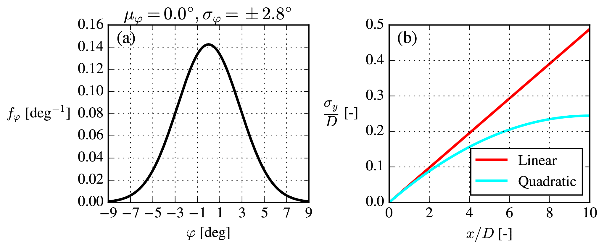
Figure C1(a) Gaussian wind direction distribution and (b) the Gaussian filter width for the convolution with σφ=2.8∘.
As discussed in Sect. 4.2 and Appendix B, the WJ-EARSM velocity deficit is rather top-hat-shaped, whereas the LES shape is more Gaussian. This could possibly be a consequence of the unidirectional inflow used in our steady RANS simulation and hence the lack of wake meandering (Larsen et al., 2008), which otherwise tends to smear out the time-averaged wake. For the k–ε–fP model it was effectively included in the turbulence model through the calibration of the CR model constant, but for the WJ-EARSM there is less room for calibration, and instead one should therefore ideally do a post-processing step to include the effect. It is however beyond the scope of this paper to carefully design such a post-processing step, but we can at least qualitatively show that the effect of wind direction uncertainty is to smoothen the top-hat-shaped wake profile into a more Gaussian shape.
The wind direction (small angle approximation) variance is
For example the hub height LES values for the V80 case gives , rad = ±2.8∘. However, according to Larsen et al. (2008) the wake meandering motion is only caused by the large eddies (the “slow-moving” part of the wind direction changes), so one should in principle use a smaller variance to model the meandering motion. However, as most of the variance is given by the large eddies, the usage of is only expected to give a small overprediction of meandering.
Assuming zero mean wind direction and a Gaussian distribution gives a simple model for the wind direction variability:
It should be intuitively clear that such a distribution of wind directions would act to smoothen out the wake profile compared to a simulation with φ=0∘, but we can also illustrate this by applying a convolution to the φ=0∘ wake profile:
To obtain fy from fφ one could simply make a change in variables from φ to y and assume σy=xσφ, but the latter assumption is equivalent to assuming that the φ=0∘ wake is moved “rigidly” from side to side, which is not realistic for at least two reasons. First, it assumes “frozen turbulence” in the sense that a wake released in the φ direction continues in that direction until infinity. Secondly, the yaw mechanism of a turbine is slower than the turbulence timescale; hence the wind direction uncertainty corresponds to yaw offsets, which will bend the wake inwards. It must therefore be presumed that σy increases more slowly than linearly in x and could for example be modeled as a quadratic polynomial instead:
The above model for σy was chosen such that it approaches the linear filter width model for , has , and is continuous; see Fig. C1. The constant −0.05 is rather arbitrary, and it must again be stressed that this is just a qualitative model to model the two aforementioned effects (one could just as well have used any other simple function to model σy).
Both the linear and quadratic filter width models are used in Gaussian convolutions of the 2D WJ-EARSM wake profiles, and the results are shown in Fig. C2. Although σφ=2.8∘ at first might appear as a small number, a significant smoothing effect is seen, which effectively removes the top-hat-shaped velocity deficits and shows that missing meandering could actually explain the top-hat shape. The linear width model overestimates the smoothing as expected from its inherent frozen turbulence assumption, while the quadratic model gives results closer to the LES. The TI results are not improved by the Gaussian convolution correction.
EllipSys3D is proprietary software of DTU.
The RANS results were generated with EllipSys3D, but the data presented can be made available by contacting the corresponding author. Interested parties are also welcome to hand-digitize the results and use them as a reference in other publications.
MB implemented the EARSM in EllipSys1D/3D, performed the RANS simulations, and wrote the initial article draft. SW provided guidance for the implementation and verification of the EARSM, MPvdL suggested re-tuning the model constants and using a Gaussian filter to compensate for the top-hat-shaped wake profiles, and MK contributed to the discussions regarding inflow turbulence in the neutral ASL. All authors (MB, SW, MPvdL, and MK) contributed to editing and finalizing the paper.
The contact author has declared that none of the authors has any competing interests.
Publisher's note: Copernicus Publications remains neutral with regard to jurisdictional claims in published maps and institutional affiliations.
The authors would like to thank Mahdi Abkar for sharing the LES data of the V80 case and Ishaan Sood and Johan Meyers for making the TotalControl LES data publicly available in an online repository. We would also like to thank the reviewers for suggestions and comments.
This paper was edited by Roland Schmehl and reviewed by J. Blair Perot and Stefano Letizia.
Apsley, D. D. and Leschziner, M. A.: A new low-Reynolds-number nonlinear two-equation turbulence model for complex flows, Int. J. Heat Fluid Flow, 19, 209–222, https://doi.org/10.1016/S0142-727X(97)10007-8, 1998. a, b, c, d, e, f, g
Bak, C., Zahle, F., Bitsche, R., Kim, T., Yde, A., Henriksen, L. C., Natarajan, A., and Hartvig Hansen, M.: Description of the DTU 10 MW Reference Wind Turbine, Tech. rep., Technical University of Denmark, https://www.hawc2.dk/download/hawc2-model/dtu-10-mw-reference-wind-turbine (last access: 26 September 2022), 2013. a
Bardina, J., Ferziger, J. H., and Reynolds, W. C.: Improved turbulence models based on large eddy simulation of homogeneous, incompressible turbulent flows, Tech. Rep. May 1983, Stanford University, http://ntrs.nasa.gov/search.jsp?R=19840009460 (last access: 26 September 2022), 1983. a, b
Bastankhah, M. and Porté-Agel, F.: A new analytical model for wind-turbine wakes, Renew Energy, 70, 116–123, https://doi.org/10.1016/j.renene.2014.01.002, 2014. a
Baungaard, M., Abkar, M., van der Laan, M. P., and Kelly, M.: A numerical investigation of a wind turbine wake in non-neutral atmospheric conditions, J. Phys.: Conf. Ser., 2265, 022015, https://doi.org/10.1088/1742-6596/2265/2/022015, 2022. a
Bechmann, A.: Perdigão CFD Grid Study, Tech. rep., Technical University of Denmark, https://orbit.dtu.dk/en/publications/perdigão-cfd-grid-study (last access: 26 September 2022), 2016. a, b
Bleeg, J., Purcell, M., Ruisi, R., and Traiger, E.: Wind farm blockage and the consequences of neglecting its impact on energy production, Energies, 11, 1609, https://doi.org/10.3390/en11061609, 2018. a
Blocken, B., Stathopoulos, T., and Carmeliet, J.: CFD simulation of the atmospheric boundary layer: wall function problems, Atmos. Environ., 41, 238–252, https://doi.org/10.1016/j.atmosenv.2006.08.019, 2007. a, b
Bottema, M.: Turbulence closure model “constants” and the problems of “inactive” atmospheric turbulence, J. Wind Eng. Indust. Aerodynam., 67-68, 897–908, https://doi.org/10.1016/S0167-6105(97)00127-X, 1997. a
Boussinesq, M. J.: Théorie de l'écoulement Tourbillonnant et Tumultueux des Liquides, Gauthier-Villars, 1897. a
Breton, S. P., Sumner, J., Sørensen, J. N., Hansen, K. S., Sarmast, S., and Ivanell, S.: A survey of modelling methods for high-fidelity wind farm simulations using large eddy simulation, Philos. T. Roy. Soc. A, 375, 1–27, https://doi.org/10.1098/rsta.2016.0097, 2017. a
Cabezón, D., Migoya, E., and Crespo, A.: Comparison of turbulence models for the computational fluid dynamics simulation of wind turbine wakes in the atmospheric boundary layer, Wind Energy, 14, 909–921, https://doi.org/10.1002/we.516, 2011. a
Crespo, A., Manuel, F., Moreno, D., Fraga, E., and Hernandez, J.: Numerical analysis of wind turbine wakes, in: Proceedings of the Delphi Workshop on Wind Energy Applications, 15–25, Delphi, https://www.academia.edu/15318618/Numerical_Analysis_of_Wind_Turbine_Wakes (last access: 26 September 2022), 1985. a
Dicholkar, A., Zahle, F., and Sørensen, N. N.: Convergence enhancement of SIMPLE-like steady-state RANS solvers applied to airfoil and cylinder flows, J. Wind Eng. Indust. Aerodynam., 220, 104863, https://doi.org/10.1016/j.jweia.2021.104863, 2022. a
Emory, M. and Iaccarino, G.: Visualizing turbulence anisotropy in the spatial domain with componentality contours, Center for Turbulence Research Annual Research Briefs, 123–137, https://web.stanford.edu/group/ctr/ResBriefs/2014/14_emory.pdf (last access: 26 September 2022), 2014. a
Emory, M., Larsson, J., and Iaccarino, G.: Modeling of structural uncertainties in Reynolds-averaged Navier–Stokes closures, Phys. Fluids, 25, 1–20, https://doi.org/10.1063/1.4824659, 2013. a, b
Feng, X., Cheng, J., Li, X., Yang, C., and Mao, Z. S.: Numerical simulation of turbulent flow in a baffled stirred tank with an explicit algebraic stress model, Chem. Eng. Sci., 69, 30–44, https://doi.org/10.1016/J.CES.2011.09.055, 2012. a
Franke, M., Wallin, S., and Thiele, F.: Assessment of explicit algebraic Reynolds-stress turbulence models in aerodynamic computations, Aerospace Sci. Technol., 9, 573–581, https://doi.org/10.1016/J.AST.2005.06.002, 2005. a
Gatski, T. B. and Speziale, C. G.: On explicit algebraic stress models for complex turbulent flows, J. Fluid Mech., 254, 59–78, https://doi.org/10.1017/S0022112093002034, 1993. a, b, c, d, e, f, g
Gavrilakis, S.: Numerical simulation of low-Reynolds-number turbulent flow through a straight square duct, J. Fluid Mech., 244, 101–129, https://doi.org/10.1017/S0022112092002982, 1992. a, b
Girimaji, S. S.: Fully explicit and self-consistent algebraic Reynolds stress model, Theor. Comput. Fluid Dynam., 8, 387–402, https://doi.org/10.1007/BF00455991, 1996. a, b, c
Gómez-Elvira, R., Crespo, A., Migoya, E., Manuel, F., and Hernández, J.: Anisotropy of turbulence in wind turbine wakes, J. Wind Eng. Indust. Aerodynam., 93, 797–814, https://doi.org/10.1016/j.jweia.2005.08.001, 2005. a, b
Heinz, S., Peinke, J., and Stoevesandt, B.: Cutting-Edge Turbulence Simulation Methods for Wind Energy and Aerospace Problems, Fluids, 6, 288, https://doi.org/10.3390/FLUIDS6080288, 2021. a
Hellsten, A. and Wallin, S.: Explicit algebraic Reynolds stress and non-linear eddy-viscosity models, Int. J. Comput. Fluid Dynam., 23, 349–361, https://doi.org/10.1080/10618560902776828, 2009. a
Hornshøj-Møller, S. D., Nielsen, P. D., Forooghi, P., and Abkar, M.: Quantifying structural uncertainties in Reynolds-averaged Navier–Stokes simulations of wind turbine wakes, Renew. Energy, 164, 1550–1558, https://doi.org/10.1016/J.RENENE.2020.10.148, 2021. a, b, c
Huser, A. and Biringen, S.: Direct Numerical Simulation of Turbulent Flow in a Square Duct, J. Fluid Mech., 257, 65–95, https://doi.org/10.1017/S002211209300299X, 1993. a
Ishihara, T. and Qian, G. W.: A new Gaussian-based analytical wake model for wind turbines considering ambient turbulence intensities and thrust coefficient effects, J. Wind Eng. Indust. Aerodynam., 177, 275–292, https://doi.org/10.1016/j.jweia.2018.04.010, 2018. a
Javadi, A. and Nilsson, H.: Detailed numerical investigation of a Kaplan turbine with rotor-stator interaction using turbulence-resolving simulations, Int. J. Heat Fluid Flow, 63, 1–13, https://doi.org/10.1016/J.IJHEATFLUIDFLOW.2016.11.010, 2017. a
Jensen, N. O.: A Note on Wind Generator Interaction, Tech. rep., Risø National Laboratory, https://orbit.dtu.dk/en/publications/a-note-on-wind-generator-interaction (last access: 26 September 2022), 1983. a, b
Jirásek, A.: Vortex-generator model and its application to flow control, J. Aircraft, 42, 1486–1491, https://doi.org/10.2514/1.12220, 2005. a
Johansson, A. V. and Wallin, S.: Reynolds Stress Model, in: Proceedings of the Sixth European Turbulence Conference, 31–34, Kluwer, Lausanne, https://doi.org/10.1007/978-94-009-0297-8_8, 1996. a, b
Larsen, G. C., Madsen, H. A., Thomsen, K., and Larsen, T. J.: Wake meandering: a pragmatic approach, Wind Energy, 11, 377–395, https://doi.org/10.1002/WE.267, 2008. a, b
Launder, B. E. and Sharma, B. I.: Application of the energy-dissipation model of turbulence to the calculation of flow near a spinning disc, Lett. Heat Mass Trans., 1, 131–137, https://doi.org/10.1016/0094-4548(74)90150-7, 1974. a
Launder, B. E. and Spalding, D. B.: The numerical computation of turbulent flows, Comput. Meth. Appl. Mech. Eng., 3, 269–289, https://doi.org/10.1016/0045-7825(74)90029-2, 1974. a, b, c
Launder, B. E., Reece, G. J., and Rodi, W.: Progress in the development of a Reynolds-stress turbulence closure, J. Fluid Mech., 68, 537–566, https://doi.org/10.1017/S0022112075001814, 1975. a, b, c
Lazeroms, W. M., Brethouwer, G., Wallin, S., and Johansson, A. V.: An explicit algebraic Reynolds-stress and scalar-flux model for stably stratified flows, J. Fluid Mech., 723, 91–125, https://doi.org/10.1017/jfm.2013.116, 2013. a, b
Lazeroms, W. M., Svensson, G., Bazile, E., Brethouwer, G., Wallin, S., and Johansson, A. V.: Study of Transitions in the Atmospheric Boundary Layer Using Explicit Algebraic Turbulence Models, Bound.-Lay. Meteorol., 161, 19–47, https://doi.org/10.1007/s10546-016-0194-1, 2016. a
Letizia, S. and Iungo, G. V.: Pseudo-2D RANS: A LiDAR-driven mid-fidelity model for simulations of wind farm flows, J. Renew. Sustain. Energ., 14, 023301, https://doi.org/10.1063/5.0076739, 2022. a
Menter, F. R., Garbaruk, A. V., and Egorov, Y.: Explicit algebraic reynolds stress models for anisotropic wall-bounded flows, in: European Conference for Aero-Space Sciences, 1–15, https://doi.org/10.1051/eucass/201203089, 2009. a, b
Menter, F. R., Garbaruk, A. V., and Egorov, Y.: Explicit algebraic reynolds stress models for anisotropic wall-bounded flows, Prog. Flight Phys., 3, 89–104, https://doi.org/10.1051/eucass/201203089, 2012. a
Michelsen, J. A.: Basis3D: A platform for development of multiblock PDE solvers, Tech. rep., Technical University of Denmark, Lyngby, https://orbit.dtu.dk/en/publications/basis3d-a-platform-for-development-of-multiblock-pde-solvers-β-re (last access: 26 September 2022), 1992. a
Munoz-Paniagua, J., García, J., and Lehugeur, B.: Evaluation of RANS, SAS and IDDES models for the simulation of the flow around a high-speed train subjected to crosswind, J. Wind Eng. Indust. Aerodynam., 171, 50–66, https://doi.org/10.1016/J.JWEIA.2017.09.006, 2017. a
Myllerup, L.: Turbulence Models for Complex Flows, PhD thesis, Technical University of Denmark, https://orbit.dtu.dk/en/publications/turbulence-models-for-complex-flows (last access: 26 September 2022), 2000. a
Nikuradse, J.: Turbulente Strömung in nicht-kreisförmigen Rohren, Ing.-Arch., 1, 306–322, 1930. a
Panofsky, H. and Dutton, J.: Atmospheric Turbulence, John Wiley & Sons, Ltd, ISBN 0471057142, 1984. a, b, c, d, e
Pirozzoli, S., Modesti, D., Orlandi, P., and Grasso, F.: Turbulence and secondary motions in square duct flow, J. Fluid Mech., 840, 631–655, https://doi.org/10.1017/JFM.2018.66, 2018. a, b, c
Pope, S. B.: A more general effective-viscosity hypothesis, J. Fluid Mech., 72, 331–340, https://doi.org/10.1017/S0022112075003382, 1975. a, b
Pope, S. B.: Turbulent Flows, Cambridge University Press, https://doi.org/10.1017/CBO9780511840531, 2000. a, b
Réthoré, P.-E.: Wind Turbine Wake in Atmospheric Turbulence, PhD thesis, Aalborg University, https://orbit.dtu.dk/en/publications/wind-turbine-wake-in-atmospheric-turbulence (last access: 26 September 2022), 2009. a, b
Réthoré, P.-E., van der Laan, P., Troldborg, N., Zahle, F., and Sørensen, N. N.: Verification and validation of an actuator disc model, Wind Energy, 17, 919–937, https://doi.org/10.1002/we.1607, 2014. a, b
Richards, P. J. and Hoxey, R. P.: Appropriate boundary conditions for computational wind engineering models using the k–ϵ turbulence model, J. Wind Eng. Indust. Aerodynam., 46-47, 145–153, https://doi.org/10.1016/0167-6105(93)90124-7, 1993. a, b, c
Richards, P. J. and Norris, S. E.: Appropriate boundary conditions for computational wind engineering models revisited, J. Wind Eng. Indust. Aerodynam., 99, 257–266, https://doi.org/10.1016/J.JWEIA.2010.12.008, 2011. a
Rodi, W.: A New Algebraic Relation for Calculating the Reynolds Stresses, Journal of Applied Mathematics and Mechanics/Zeitschrift für Angewandte Mathematik und Mechanik, 56, T219–T221, https://doi.org/10.1002/ZAMM.19765613093, 1976. a, b
Shabbir, A. and Shih, T.-H.: Critical assessment of Reynolds stress turbulence models using homogeneous flows, in: NASA TM 105954, https://doi.org/10.2514/6.1993-82, 1993. a
Sogachev, A. and Kelly, M.: Consistent Two-Equation Closure Modelling for Atmospheric Research: Buoyancy and Vegetation Implementations, Bound.-Lay. Meteorol., 145, 307–327, https://doi.org/10.1007/s10546-012-9726-5, 2012. a
Sood, I. and Meyers, J.: Reference Windfarm database PDk 90 (Version 1), Zenodo [data set], https://doi.org/10.5281/zenodo.3688716, 2020. a
Sørensen, N. N.: General purpose flow solver applied to flow over hills, PhD thesis, Technical University of Denmark, https://orbit.dtu.dk/en/publications/general-purpose-flow-solver-applied-to-flow-over-hills (last access: 26 September 2022), 1995. a, b, c, d, e, f, g
Sørensen, N. N., Bechmann, A., Johansen, J., Myllerup, L., Botha, P., Vinther, S., and Nielsen, B. S.: Identification of severe wind conditions using a Reynolds Averaged Navier–Stokes solver, J. Phys. Conf. Ser., 75, 012053, https://doi.org/10.1088/1742-6596/75/1/012053, 2007. a, b
Taulbee, D. B.: An improved algebraic Reynolds stress model and corresponding nonlinear stress model, Phys. Fluids A, 4, 2555–2561, https://doi.org/10.1063/1.858442, 1992. a, b, c, d, e, f
Tavoularis, S. and Corrsin, S.: Experiments in nearly homogenous turbulent shear flow with a uniform mean temperature gradient. Part 1, J. Fluid Mech., 104, 311–347, https://doi.org/10.1017/S0022112081002930, 1981. a
Thompson, J. F., Warsi, Z. U. A., and Mastin, C. W.: Numerical Grid Generation: Foundations and Applications, in: 1st Edn., ISBN 044400985X, North-Holland, 1985. a, b
Tian, L., Song, Y., Zhao, N., Shen, W., and Wang, T.: AD/RANS simulations ofwind turbinewake flow employing the RSM turbulence model: Impact of isotropic and anisotropic inflow conditions, Energies, 12, 1–14, https://doi.org/10.3390/en12214026, 2019. a
Troldborg, N., Sørensen, N. N., Réthoré, P.-E., and van der Laan, M. P.: A consistent method for finite volume discretization of body forces on collocated grids applied to flow through an actuator disk, Comput. Fluids, 119, 197–203, https://doi.org/10.1016/J.COMPFLUID.2015.06.028, 2015. a
van der Laan, M. P.: Efficient Turbulence Modeling for CFD Wake Simulations, PhD thesis, Technical University of Denmark, https://orbit.dtu.dk/en/publications/efficient-turbulence-modeling-for-cfd-wake-simulations (last access: 26 September 2022), 2014. a, b, c, d, e, f, g, h, i, j, k, l, m, n, o, p, q
van der Laan, M. P. and Andersen, S. J.: The turbulence scales of a wind turbine wake: A revisit of extended k–ϵ models, J. Phys.: Conf. Ser., 1037, 072001, https://doi.org/10.1088/1742-6596/1037/7/072001, 2018. a
van der Laan, M. P., Sørensen, N. N., Réthoré, P.-E., Mann, J., Kelly, M. C., and Troldborg, N.: The k–ϵ-fp model applied to double wind turbine wakes using different actuator disk force methods, Wind Energy, 18, 2223–2240, https://doi.org/10.1002/we.1816, 2015a. a, b
van der Laan, M. P., Sørensen, N. N., Réthoré, P. E., Mann, J., Kelly, M. C., Troldborg, N., Schepers, J. G., and Machefaux, E.: An improved k–ϵ model applied to a wind turbine wake in atmospheric turbulence, Wind Energy, 18, 889–907, https://doi.org/10.1002/we.1736, 2015b. a, b
van der Laan, P., Sørensen, N. N., Réthoré, P.-E., Mann, J., Kelly, M. C., Troldborg, N., Hansen, K. S., and Murcia, J. P.: The k–ϵ-fp model applied to wind farms, Wind Energy, 18, 2065–2084, https://doi.org/10.1002/we.1804, 2015c. a
van der Laan, M. P., Baungaard, M., and Kelly, M.: Inflow modeling for wind farm flows in RANS, J. Phys.: Conf. Ser., 1934, 012012, https://doi.org/10.1088/1742-6596/1934/1/012012, 2021. a
van der Laan, P. and Sørensen, N. N.: A 1D version of EllipSys, Tech. rep., Technical University of Denmark, https://orbit.dtu.dk/en/publications/a-1d-version-of-ellipsys(2b589155-4305-496c-8513-c12da7f4 (last access: 26 September 2022), 2017. a
Wallin, S.: Engineering turbulence modelling for CFD with a focus on explicit algebraic Reynolds stress models by, PhD thesis, KTH Royal Institute of Technology, http://www.mech.kth.se/thesis/2000/phd/phd_2000_stefan_wallin.pdf (last access: 26 September 2022), 2000. a
Wallin, S. and Johansson, A. V.: An explicit algebraic Reynolds stress model for incompressible and compressible turbulent flows, J. Fluid Mech., 403, 89–132, https://doi.org/10.1017/S0022112099007004, 2000. a, b, c, d, e, f, g, h, i, j, k, l, m, n, o, p, q, r
Wallin, S. and Johansson, A. V.: Modelling streamline curvature effects in explicit algebraic Reynolds stress turbulence models, Int. J. Heat Fluid Flow, 23, 721–730, https://doi.org/10.1016/S0142-727X(02)00168-6, 2002. a, b
Weaver, D. and Mišković, S.: A study of RANS turbulence models in fully turbulent jets: A perspective for CFD-DEM simulations, Fluids, 6, 1–19, https://doi.org/10.3390/fluids6080271, 2021. a
Wu, J. L., Wang, J. X., and Xiao, H.: A Bayesian Calibration–Prediction Method for Reducing Model-Form Uncertainties with Application in RANS Simulations, Flow Turbul. Combust., 97, 761–786, https://doi.org/10.1007/s10494-016-9725-6, 2016. a
Wyngaard, J. C.: Turbulence in the Atmosphere, Cambridge University Press, ISBN 9780511840524, 2010. a
Ying, R. and Canuto, V. M.: Turbulence Modelling Over Two-Dimensional Hills Using An Algebraic Reynolds Stress Expression, Bound.-Lay. Meteorol., 77, 69–99, https://doi.org/10.1007/BF00121859, 1996. a, b
Želi, V., Brethouwer, G., Wallin, S., and Johansson, A. V.: Consistent Boundary-Condition Treatment for Computation of the Atmospheric Boundary Layer Using the Explicit Algebraic Reynolds-Stress Model, Bound.-Lay. Meteorol., 171, 53–77, https://doi.org/10.1007/s10546-018-0415-x, 2019. a
Želi, V., Brethouwer, G., Wallin, S., and Johansson, A. V.: Modelling of Stably Stratified Atmospheric Boundary Layers with Varying Stratifications, Bound.-Lay. Meteorol., 176, 229–249, https://doi.org/10.1007/s10546-020-00527-8, 2020. a, b
Želi, V., Brethouwer, G., Wallin, S., and Johansson, A. V.: Explicit Algebraic Reynolds-stress Modelling of a Convective Atmospheric Boundary Layer Including Counter-Gradient Fluxes, Bound.-Lay. Meteorol., 178, 487–497, https://doi.org/10.1007/s10546-020-00580-3, 2021. a
- Abstract
- Introduction
- Turbulence modeling
- Verification cases
- Single-wind-turbine wake
- Aligned row of wind turbines
- Conclusions
- Appendix A: Grid study of WJ-EARSM for wind turbine wake simulations
- Appendix B: Tuning the turbulence model constants in the WJ-EARSM
- Appendix C: Effect of wind direction uncertainty
- Code availability
- Data availability
- Author contributions
- Competing interests
- Disclaimer
- Acknowledgements
- Review statement
- References