Flight trajectory optimization of Fly-Gen airborne wind energy systems through a harmonic balance method

The optimal control problem for flight trajectories of Fly-Gen airborne wind energy systems (AWESs) is a crucial research topic for the field, as suboptimal paths can lead to a drastic reduction in power production. One of the novelties of the present work is the expression of the optimal control problem in the frequency domain through a harmonic balance formulation. This allows the potential reduction of the problem size by solving only for the main harmonics and allows the implicit imposition of periodicity of the solution. The trajectory is described by the Fourier coefficients of the dynamics (elevation and azimuth angles) and of the control inputs (onboard wind turbine thrust and AWES roll angle). To isolate the effects of each physical phenomenon, optimal trajectories are presented with an increasing level of physical representation from the most idealized case: (i) if the mean thrust power (mechanical power linked to the dynamics) is considered as the objective function, optimal trajectories are characterized by a constant AWES velocity over the loop and a circular shape. This is done by converting all the gravitational potential energy into electrical energy. At low wind speed, onboard wind turbines are then used as propellers in the ascendant part of the loop; (ii) if the mean shaft power (mechanical power after momentum losses) is the objective function, a part of the potential energy is converted into kinetic and the rest into electrical energy. Therefore, the AWES velocity fluctuates over the loop; (iii) if the mean electrical power is considered as the objective function, the onboard wind turbines are never used as propellers because of the power conversion efficiency. Optimal trajectories for case (ii) and (iii) have a circular shape squashed along the vertical direction. The optimal control inputs can be generally modeled with one harmonic for the onboard wind turbine thrust and two for AWES roll angle without a significant loss of power, demonstrating that the absence of high-frequency control is not detrimental to the power generated by Fly-Gen AWESs.

1 Introduction

Airborne wind energy (AWE) is the branch of wind energy which aims at harvesting energy from the wind using airborne systems. Airborne wind energy systems can be classified according to the flight operations, which are linked to the power generation technique. The flight operations can be divided into crosswind, tether-aligned and rotational, as discussed by Vermillion et al. (2021). Electrical power can be generated by a fixed or a moving ground station, or, alternatively, it can be directly generated on board and transmitted to the ground through the tether. The wing type, soft or fixed, additionally classifies the AWES. This paper focuses on AWESs based on a fixed-wing with onboard generation, known as Fly-Gen AWESs. However, the methods developed can be applied to other AWE architectures, after an appropriate rework of the dynamic models. These methods are suitable for investigating the optimal trajectories of AWESs and, especially when applied to low-fidelity models, for understanding their physical characteristics. The interpretation of the physical characteristics of optimal trajectories and the analysis of how they are influenced by parameters describing the system and its operation is the main goal of this work. With this aim, solutions are compared with analytical results coming from first-principle models whenever possible.

The first analytical power equation of crosswind AWESs was derived by Loyd (1980), and additional refinements, such as the one proposed by Trevisi et al. (2020a), made an effort to modify analytic equations to include gravitational and centrifugal effects. This kind of analytical models can be used to study how power and other relevant trends approximately scale with design parameters. However, they typically neglect the system dynamics and its effect on power generation. These effects can be studied with dynamical models, ranging from low to high fidelity. Typically, low- to mid-fidelity models are used to investigate optimal trajectories of AWE. Low-fidelity dynamic models are characterized by multiple assumptions, which simplify the models, and by the low computational cost. The quasi-steady model (van der Vlugt et al., 2019) assumes the kite as a point mass in steady state for each point of the loop. This model is validated with experimental data (Schelbergen and Schmehl, 2020), and it is considered accurate for soft kites, where the inertia is low and the AWES quickly reaches the steady state. A similar approach is considered while deriving the Unicycle model (Fagiano et al., 2014; Vermillion et al., 2021). Also this model, based on a point mass, is developed for soft-wing AWESs and computes the velocity vector via quasi-steady flight equations. The kite orientation is found by a turning law that is derived from lateral force equilibrium and is validated through a number of experiments. The Unifoil model (Cobb et al., 2020) is derived by modification of the Unicycle model in order to be applied to fixed-wing AWESs. Indeed, the quasi-steady assumption is removed, and the turning maneuvers are modeled with a yaw dynamic equation.

Higher-fidelity, but still computationally efficient, dynamic models are developed by Sánchez-Arriaga et al. (2017, 2019); Sánchez-Arriaga and Serrano-Iglesias (2021) as a part of the Lagrangian Kite Flight Simulators (LAKSA) package based on minimal coordinates and by Gros and Diehl (2013) to study the dynamics of multiple AWES configurations. Moreover, thorough Newtonian dynamic models are used to compute reference flight paths and the consequent flight path control for soft-wing AWESs (Fechner et al., 2015; Fechner and Schmehl, 2016) and for fixed-wing AWESs (Licitra et al., 2019; Malz et al., 2019; Eijkelhof and Schmehl, 2022).

The dynamic models just introduced are particularly suitable to be used within optimal control studies for their computational inexpensiveness and for the reduced number of nonlinearities compared to even higher-fidelity codes, such as kiteFAST (Jonkman et al., 2018). The Unicycle and Unifoil models, introduced earlier, are mainly used to compute reference flight paths and for flight path control development (Cobb et al., 2020; Fernandes et al., 2021). To ease the deployment of optimal control problems for AWE, awebox (awebox, 2022) is developed and used, for instance by Leuthold et al. (2018), Haas et al. (2019) and De Schutter et al. (2019), to solve optimal control problems. awebox solves optimal control problems in time, imposing periodicity constraints. A similar optimal control problem is studied by Horn et al. (2013) and Malz et al. (2020a, b), where the optimal trajectory is found in time using a discretization by direct collocation and a homotopy strategy based on the relaxation of the dynamic constraints (Gros et al., 2013). Licitra et al. (2019) solve an optimal control problem with an experimentally validated dynamic model of a Ground-Gen AWES. They find that, under some prescribed constraints, circular and figure-of-eight trajectories produce similar mean power and that closed-loop control enhances robustness but decreases power production by about 10 %. Control in all operation phases is studied by Rapp et al. (2019) and Todeschini et al. (2021): the present work can be understood as a study of the guidance (or the reference trajectory) used during the power generation phase of their study.

Pasquinelli (2021) investigates the power losses in a circular trajectory with a dynamical quasi-analytical model. He finds that the causes of power losses are mainly two: the AWES span non-perpendicularity with respect to the incoming wind during the motion and the AWES speed fluctuation over the loop. The Makani team (Tucker, 2020) studies the flight trajectories of Fly-Gen AWESs with a simplified quasi-analytical approach, aiming at describing their physical characteristics. They run their flight simulator for different trajectories and production strategies to derive analytical expressions, which can describe the consequences of different operational choices. Their production strategy at low wind speed is to convert part of the potential energy into kinetic and part into electrical, when the AWES moves downward. To reduce the potential energy exchange, they suggest to squash the trajectories along the vertical direction. Moreover, they explain that using electrical power to push the AWES upward drastically decreases the overall power production, as power needs to be converted from mechanical to electrical and again from electrical to mechanical, so that the related efficiencies are counted twice. They, in accord with the study for Ground-Gen by Stuyts et al. (2015), conclude that the electrical conversion losses should be considered when deciding on the production strategy. Following these conclusions, the present work also investigates the influence of the power generation efficiencies on the optimal trajectories.

As the aim of this work is to interpret optimal trajectories in a physical way, a low-fidelity dynamic model, similar to the one proposed by Fernandes et al. (2021) (reformulated for Fly-Gen AWESs), is selected. Instead of solving the dynamics and the optimal control problem in time, the present approach models the problem in the frequency domain, making use of a harmonic balance method, which expands the periodic solution as a Fourier series (Lau et al., 1982; Pierre and Dowell, 1985; Dimitriadis, 2017). Working with the Fourier coefficients and not with the time series themselves allows the potential reduction of the problem size depending on the problem at hand, the search for periodic solutions implicitly and the study of the solution in an intuitive way by looking at the contribution of the different harmonics. To the best of the authors' knowledge, this is the first work on AWESs where an optimal control problem aided by a harmonic balance methodology is formulated.

Even though the frequency-domain formulation can be used for any periodic flight trajectories (i.e., circular and figure of eight), only circular trajectories are analyzed here to limit the paper scope and length. Figure-of-eight trajectories are intended to be analyzed and intensively compared with circular trajectories in a future work.

The paper is organized as follows: in Sect. 2 the flight dynamic model, the harmonic balance and the optimal control statement are introduced. In Sect. 3, the main results from steady-state analytical models are recalled from literature, together with the introduction of some key non-dimensional numbers used later in the analyses. In Sect. 4, the solution obtained with the harmonic balance formulation is validated against the time integration. In Sect. 5, optimal control problems with constant wind inflow and no constraints on the mean elevation angle are analyzed. This extreme idealization allows the understanding of some optimal trajectory characteristics which are also present in more realistic cases. Section 6 focuses on the results of a more realistic optimal control problem where the wind shear and a constraint on the minimum elevation angle are included in the analyses. Finally, in Sect. 7 the results are discussed and the main conclusions summarized.

2 Methodology

2.1 Flight dynamic model

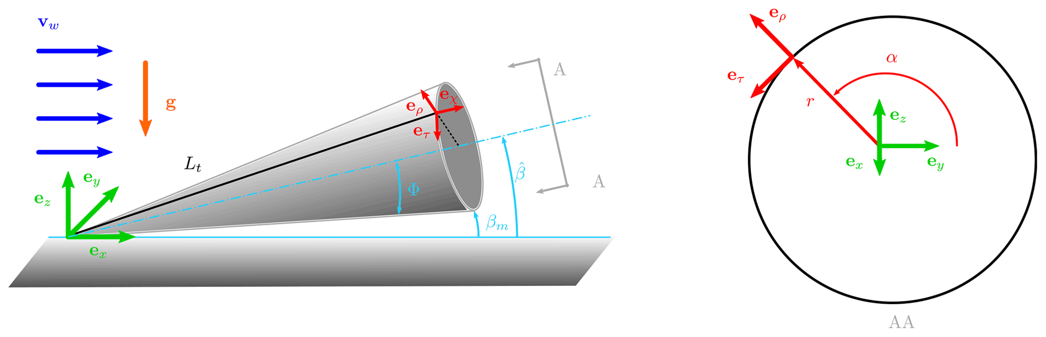
Two coordinate systems (Fig. 1a) are defined to derive the equations of motion. The ground coordinate system (denoted by ℱ_G) is inertial and centered at the ground station: e_x points downwind, e_z toward the zenith and e_y completes the right-handed frame. For convenience, spherical coordinates are used to describe the position of the airborne unit, with L_t the tether length, ϕ the azimuth angle and β the elevation angle. The spherical reference frame (denoted by ℱ_S) is unequivocally defined at every position with the origin at the AWES center of mass, e_r pointing outward the sphere in the radial direction, e_ϕ normal to e_r and contained on a plane parallel to x–y, and ${\mathit{e}}_{\mathit{\beta }}={\mathit{e}}_{\mathrm{r}}\times {\mathit{e}}_{\mathit{\varphi }}$. The position p, velocity v and acceleration a vectors projected into the spherical reference frame ℱ_S are

$$\begin{array}{}\text{(1)}& \begin{array}{rl}& \mathit{p}=L_{\mathrm{t}}{\mathit{e}}_{\mathrm{r}},\\ & \mathit{v}=L_{\mathrm{t}}\dot{\mathit{\varphi }}\cos \mathit{\beta }{\mathit{e}}_{\mathit{\varphi }}+L_{\mathrm{t}}\dot{\mathit{\beta }}{\mathit{e}}_{\mathit{\beta }},\\ & \mathit{a}=\left(-L_{\mathrm{t}}{\dot{\mathit{\varphi }}}^{\mathrm{2}}{\cos }^{\mathrm{2}}\mathit{\beta }-L_{\mathrm{t}}{\dot{\mathit{\beta }}}^{\mathrm{2}}\right){\mathit{e}}_{\mathrm{r}}\\ & +\left(L_{\mathrm{t}}\ddot{\mathit{\varphi }}\cos \mathit{\beta }-\mathrm{2}{L}_{\mathrm{t}}\dot{\mathit{\varphi }}\dot{\mathit{\beta }}\sin \mathit{\beta }\right){\mathit{e}}_{\mathit{\varphi }}\\ & +\left(L_{\mathrm{t}}{\dot{\mathit{\beta }}}^{\mathrm{2}}\sin \mathit{\beta }\cos \mathit{\beta }+L_{\mathrm{t}}\ddot{\mathit{\beta }}\right){\mathit{e}}_{\mathit{\beta }}.\end{array}\end{array}$$

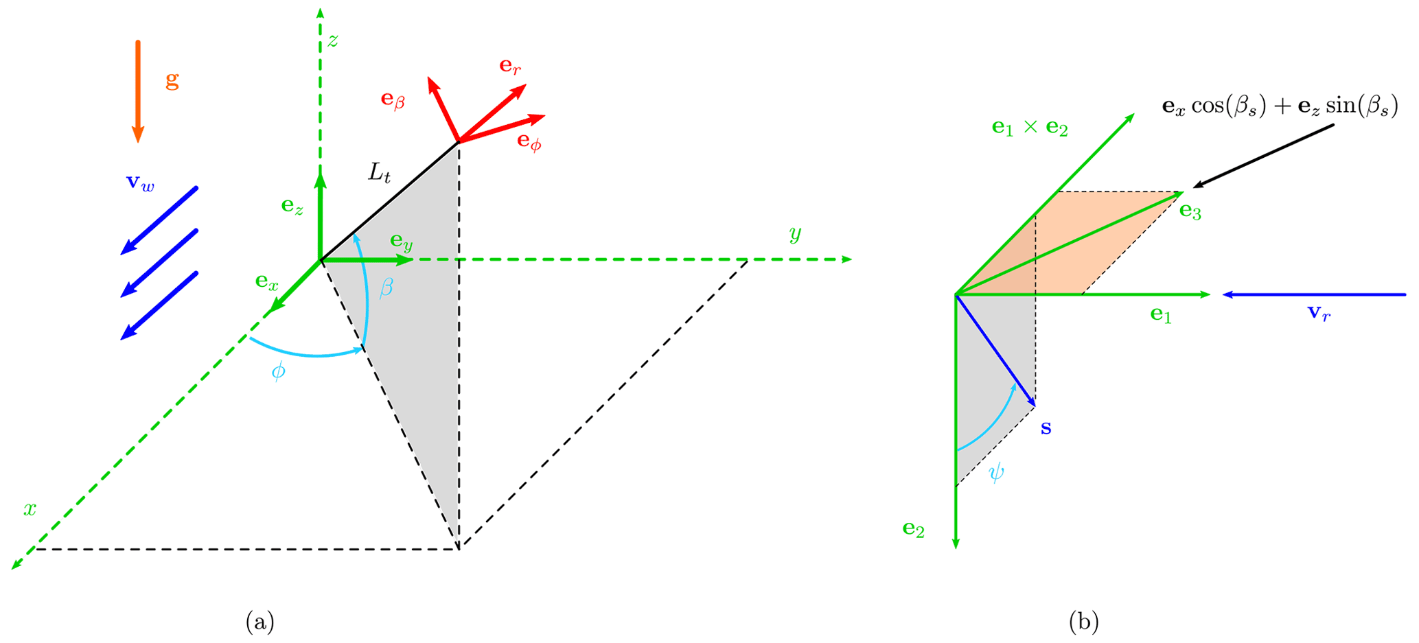
Figure 1 (a) Ground reference frame ℱ_G (${\mathit{e}}_x-{\mathit{e}}_y-{\mathit{e}}_z$) and spherical reference frame ℱ_S (${\mathit{e}}_{\mathrm{r}}-{\mathit{e}}_{\mathit{\varphi }}-{\mathit{e}}_{\mathit{\beta }}$) and (b) sketch for the spanwise unit vector s definition.

The wind velocity is in the positive x-axis direction of ℱ_G, and projected into the spherical reference frame is

$$\begin{array}{}\text{(2)}& \begin{array}{rl}& {\mathit{v}}_{\mathrm{w}}=v_{\mathrm{w}}\left(\cos \mathit{\varphi }\cos \mathit{\beta }{\mathit{e}}_{\mathrm{r}}-\sin \mathit{\varphi }{\mathit{e}}_{\mathit{\varphi }}-\cos \mathit{\varphi }\sin \mathit{\beta }{\mathit{e}}_{\mathit{\beta }}\right),\\ & v_{\mathrm{w}}\left(h\right)=v_{\mathrm{w},\mathrm{0}}{\left({\displaystyle \frac{h}{h_{\mathrm{0}}}}\right)}^{{\mathit{\alpha }}_{\mathrm{s}}}=v_{\mathrm{w},\mathrm{0}}{\left({\displaystyle \frac{L_{\mathrm{t}}}{h_{\mathrm{0}}}}\sin \mathit{\beta }\right)}^{{\mathit{\alpha }}_{\mathrm{s}}},\end{array}\end{array}$$

where the wind speed v_w as function of the altitude h is modeled with an exponential law: v_w,0 is the reference wind speed at the reference altitude h₀ and α_s is the wind shear exponent. The relative speed between the AWES and the wind is

$$\begin{array}{}\text{(3)}& {\mathit{v}}_{\mathrm{r}}={\mathit{v}}_{\mathrm{w}}-\mathit{v}.\end{array}$$

To describe the AWES attitude, a non-sideslip velocity constraint is included in the modeling. Indeed, the wing operates at the highest performance under this condition. To impose this constraint implicitly, the unit vector e₁ is defined to point to the direction opposite to the relative wind speed:

$$\begin{array}{}\text{(4)}& {\mathit{e}}_{\mathrm{1}}=-{\displaystyle \frac{{\mathit{v}}_{\mathrm{r}}}{\left|{\mathit{v}}_{\mathrm{r}}\right|}}.\end{array}$$

The spanwise unit vector s (with origin at the center of mass and pointing in the right-wing span direction) is defined perpendicular to e₁ with the procedure illustrated in Fig. 1b. A second vector e₃ is defined as a unit vector in a plane parallel to the x–z plane with elevation β_s (and negative sign):

$$\begin{array}{}\text{(5)}& \begin{array}{rl}& {\mathit{e}}_{\mathrm{3}}=-\left({\mathit{e}}_x\cos \left({\mathit{\beta }}_{\mathrm{s}}\right)+{\mathit{e}}_z\sin \left({\mathit{\beta }}_{\mathrm{s}}\right)\right),\\ & {\mathit{e}}_x=\cos \mathit{\varphi }\cos \mathit{\beta }{\mathit{e}}_{\mathrm{r}}-\sin \mathit{\varphi }{\mathit{e}}_{\mathit{\varphi }}-\cos \mathit{\varphi }\sin \mathit{\beta }{\mathit{e}}_{\mathit{\beta }},\\ & {\mathit{e}}_z=\sin \mathit{\beta }{\mathit{e}}_{\mathrm{r}}+\cos \mathit{\beta }{\mathit{e}}_{\mathit{\beta }}.\end{array}\end{array}$$

Note that e₃ points upwind when β_s=0. The unit vector e₂ is then defined as

$$\begin{array}{}\text{(6)}& {\mathit{e}}_{\mathrm{2}}={\displaystyle \frac{{\mathit{e}}_{\mathrm{3}}\times {\mathit{e}}_{\mathrm{1}}}{|{\mathit{e}}_{\mathrm{3}}\times {\mathit{e}}_{\mathrm{1}}|}},\end{array}$$

where $|{\mathit{e}}_{\mathrm{3}}\times {\mathit{e}}_{\mathrm{1}}|$ can take values smaller than one because e₃ and e₁ are not defined to be perpendicular in general. In this way, e₂ is perpendicular to the plane e₃–e₁. Rodrigues' formula is then used to define s through a rotation of ψ around e₁, starting from e₂:

$$\begin{array}{}\text{(7)}& \mathit{s}={\mathit{e}}_{\mathrm{2}}\cos \mathit{\psi }+\left({\mathit{e}}_{\mathrm{1}}\times {\mathit{e}}_{\mathrm{2}}\right)\sin \mathit{\psi }+{\mathit{e}}_{\mathrm{1}}\left({\mathit{e}}_{\mathrm{1}}\cdot {\mathit{e}}_{\mathrm{2}}\right)(\mathrm{1}-\cos \mathit{\psi }).\end{array}$$

With this formulation, s is defined to be always perpendicular to the relative wind, and its components are defined by a unique angle ψ, called hereafter roll angle. When ψ=0, s is perpendicular to e₃.

The aerodynamic lift L and the drag D take the standard form

$$\begin{array}{}\text{(8)}& \mathit{L}={\displaystyle \frac{\mathrm{1}}{\mathrm{2}}}\mathit{\rho }A{C}_{\mathrm{L}}\left|{\mathit{v}}_{\mathrm{r}}\right|{\mathit{v}}_{\mathrm{r}}\times \mathit{s},\mathit{D}={\displaystyle \frac{\mathrm{1}}{\mathrm{2}}}\mathit{\rho }A{C}_{\mathrm{D}}\left|{\mathit{v}}_{\mathrm{r}}\right|{\mathit{v}}_{\mathrm{r}},\end{array}$$

where ρ is the air density, A is the wing area, and the lift and drag coefficients C_L and C_D are considered constant. The drag coefficient C_D includes the contribution from the tether drag (Trevisi et al., 2020a). The gravitational force F_g and the tether force T are

$$\begin{array}{}\text{(9)}& {\mathit{F}}_{\mathrm{g}}=-mg\left(\sin \mathit{\beta }{\mathit{e}}_{\mathrm{r}}+\cos \mathit{\beta }{\mathit{e}}_{\mathit{\beta }}\right),\mathit{T}=-T{\mathit{e}}_{\mathrm{r}},\end{array}$$

where m is the AWES mass, g is the gravitational acceleration and T is the norm of the tether force. The thrust produced by the onboard wind turbines D_t is expressed as a linear function of the aerodynamic drag with gain γ:

$$\begin{array}{}\text{(10)}& {\mathit{D}}_{\mathrm{t}}=\mathit{\gamma }\mathit{D}.\end{array}$$

The dynamic equations of motion in compact form read

$$\begin{array}{}\text{(11)}& m\mathit{a}=\mathit{L}+\mathit{D}+{\mathit{D}}_{\mathrm{t}}+{\mathit{F}}_{\mathrm{g}}+\mathit{T},\end{array}$$

recalling that a is given by Eq. (1).

As the objectives of the optimal control problems are linked to the power production, three different power quantities are defined. The thrust power P_t (i.e., the power linked to the AWES dynamics) is estimated as a dot product of D_t and the relative velocity:

$$\begin{array}{}\text{(12)}& P_{\mathrm{t}}={\mathit{D}}_{\mathrm{t}}\cdot {\mathit{v}}_{\mathrm{r}}.\end{array}$$

The shaft power P_s (i.e., the mechanical power that can be converted to electrical power) is modeled using 1D momentum theory (actuator disc) as

$$\begin{array}{}\text{(13)}& P_{\mathrm{s}}=(\mathrm{1}-a)P_{\mathrm{t}}=\left({\displaystyle \frac{\mathrm{1}}{\mathrm{2}}}+{\displaystyle \frac{\mathrm{1}}{\mathrm{2}}}\sqrt{\mathrm{1}-\mathit{\gamma }{C}_{\mathrm{D}}{\displaystyle \frac{A}{A_{\mathrm{t}}}}}\right)P_{\mathrm{t}},\end{array}$$

where the induction a is found by setting the thrust given by momentum theory (${\mathit{T}}_{\mathrm{d}}=\frac{\mathrm{1}}{\mathrm{2}}\mathit{\rho }{A}_{\mathrm{t}}\left(\mathrm{4}a\right(\mathrm{1}-a\left)\right)\left|{\mathit{v}}_{\mathrm{r}}\right|{\mathit{v}}_{\mathrm{r}}$) equal to D_t, as in Trevisi et al. (2020b), and A_t is the total turbine area.

Finally, the electrical power exchanged with the grid P takes into account the generator and transmission efficiency η_el:

$$\begin{array}{}\text{(14)}& P=\left\{\begin{array}{cl}{P}_{\mathrm{s}}-\left(\mathrm{1}-{\mathit{\eta }}_{\mathrm{el}}\right)P_{\mathrm{s}}& \mathrm{for}\mathit{\gamma }\ge \mathrm{0}\\ P_{\mathrm{s}}+\left(\mathrm{1}-{\mathit{\eta }}_{\mathrm{el}}\right)P_{\mathrm{s}}& \mathrm{for}\mathit{\gamma }<\mathrm{0}\end{array}\right..\end{array}$$

When power is generated (γ>0), the electrical power distributed to the grid P is lower than the shaft power P_s because of electrical efficiencies. When power from the grid is used, the electrical power requested to the grid P is instead higher in absolute value compared to the shaft power P_s. To model the discontinuity in a continuous optimization framework, the logistic function is used:

$$\begin{array}{}\text{(15)}& P=P_{\mathrm{s}}-\left({\displaystyle \frac{\mathrm{1}-e^{-f\mathit{\gamma }}}{\mathrm{1}+e^{-f\mathit{\gamma }}}}\right)\left(\mathrm{1}-{\mathit{\eta }}_{\mathrm{el}}\right)P_{\mathrm{s}},\end{array}$$

where f is taken equal to 100.

2.2 Frequency-domain formulation

Frequency-domain formulations may present clear advantages when solving for periodic solutions of dynamic and control problems. They have the capability of solving for both stable and unstable branches of periodic solutions in an efficient way. Moreover, they potentially use fewer variables to describe the same problems. Since the problem of optimal trajectories for AWESs has a periodic nature, the flight dynamic model just introduced is expressed in the frequency domain. The harmonic balance methodology is then used to transform the differential equations of motion into a set of nonlinear algebraic equations (Dimitriadis, 2017). The equations of motion (Eq. 11) can be written as a set of second-order nonlinear differential equations in the form

$$\begin{array}{}\text{(16)}& \begin{array}{rl}& \mathbf{f}(\mathit{x},\dot{\mathit{x}},\ddot{\mathit{x}},\mathit{u})=\mathbf{0},\\ & \mathit{x}={\left[\begin{array}{c}\mathit{\beta }\left(t\right),\mathit{\varphi }\left(t\right)\end{array}\right]}^T,\mathit{u}={\left[\begin{array}{c}\mathit{\psi }\left(t\right),\mathit{\gamma }\left(t\right)\end{array}\right]}^T,\end{array}\end{array}$$

where x is the state vector and u is the control vector. By assuming that Eq. (16) accepts periodic solutions, every variable of the state vector is expanded as a Fourier series of order N_x:

$$\begin{array}{}\text{(17)}& \begin{array}{rl}& x\left(t\right)\approx {\displaystyle \frac{X_{\mathrm{0}}}{\mathrm{2}}}+\sum _{k=\mathrm{1}}^{N_x}{X}_{k,\mathrm{s}}\sin \left(k\mathit{\omega }t\right)+X_{k,\mathrm{c}}\cos \left(k\mathit{\omega }t\right),\\ & \mathbf{X}={\left[\begin{array}{c}{X}_{\mathrm{0}},X_{\mathrm{1},\mathrm{s}},X_{\mathrm{2},\mathrm{s}},\mathrm{\dots }{X}_{\mathrm{1},\mathrm{c}},X_{\mathrm{2},\mathrm{c}},\mathrm{\dots }\end{array}\right]}^T,\end{array}\end{array}$$

with $\mathit{\omega }=\frac{\mathrm{2}\mathit{\pi }}{\mathcal{T}}$ being the fundamental frequency of the motion and 𝒯 the period. Alternatively, the state vector can be expressed as

$$\begin{array}{}\text{(18)}& \begin{array}{rl}& x\left(t\right)\approx {\displaystyle \frac{A_{\mathrm{0}}}{\mathrm{2}}}+\sum _{k=\mathrm{1}}^{N_x}{A}_k\cos \left(k\mathit{\omega }t-{\mathit{\theta }}_k\right),\\ & \mathbf{A}={\left[\begin{array}{c}{A}_{\mathrm{0}},A_{\mathrm{1}},\mathrm{\dots }\end{array}\right]}^T,\mathit{\theta }={\left[\begin{array}{c}{\mathit{\theta }}_{\mathrm{1}},{\mathit{\theta }}_{\mathrm{2}},\mathrm{\dots }\end{array}\right]}^T,\end{array}\end{array}$$

where

$$\begin{array}{}\text{(19)}& A_{\mathrm{0}}=X_{\mathrm{0}},A_k=\sqrt{X_{k,\mathrm{s}}^{\mathrm{2}}+X_{k,\mathrm{c}}^{\mathrm{2}}},{\mathit{\theta }}_k=\arctan \left({\displaystyle \frac{X_{k,\mathrm{s}}}{X_{k,\mathrm{c}}}}\right).\end{array}$$

The first and second time derivatives of the state vector can be found analytically:

$$\begin{array}{}\text{(20)}& \begin{array}{rl}& \dot{x}\left(t\right)\approx \sum _{k=\mathrm{1}}^{N_x}k\mathit{\omega }\left(X_{k,\mathrm{s}}\cos \left(k\mathit{\omega }t\right)-X_{k,\mathrm{c}}\sin \left(k\mathit{\omega }t\right)\right),\\ & \ddot{x}\left(t\right)\approx -\sum _{k=\mathrm{1}}^{N_x}(k\mathit{\omega }{)}^{\mathrm{2}}\left(X_{k,\mathrm{s}}\sin \left(k\mathit{\omega }t\right)+X_{k,\mathrm{c}}\cos \left(k\mathit{\omega }t\right)\right).\end{array}\end{array}$$

Similarly, the control inputs, assumed to be periodic, can also be expressed as a Fourier series of order N_u:

$$\begin{array}{}\text{(21)}& \begin{array}{rl}& u\left(t\right)\approx {\displaystyle \frac{U_{\mathrm{0}}}{\mathrm{2}}}+\sum _{k=\mathrm{1}}^{N_u}{U}_{k,\mathrm{s}}\sin \left(k\mathit{\omega }t\right)+U_{k,\mathrm{c}}\cos \left(k\mathit{\omega }t\right),\\ & \mathbf{U}={\left[\begin{array}{c}{U}_{\mathrm{0}},U_{\mathrm{1},\mathrm{s}},U_{\mathrm{2},\mathrm{s}},\mathrm{\dots }{U}_{\mathrm{1},\mathrm{c}},U_{\mathrm{2},\mathrm{c}},\mathrm{\dots }\end{array}\right]}^T,\end{array}\end{array}$$

where N_u<N_x because the equations of motion need to be solved at frequencies higher than the control inputs order. By introducing Eqs. (17), (20) and (21) into Eq. (16), the equations of motion can be expanded as a Fourier series of order N_x:

$$\begin{array}{}\text{(22)}& \begin{array}{rl}\mathbf{f}\left({\mathbf{X}}_{\mathit{\beta }},{\mathbf{X}}_{\mathit{\varphi }},{\mathbf{U}}_{\mathit{\psi }},{\mathbf{U}}_{\mathit{\gamma }},\mathit{\omega },t\right)& \approx {\displaystyle \frac{{\mathbf{F}}_{\mathrm{0}}}{\mathrm{2}}}+\sum _{k=\mathrm{1}}^{N_x}{\mathbf{F}}_{k,\mathrm{s}}\sin \left(k\mathit{\omega }t\right)\\ & +{\mathbf{F}}_{k,\mathrm{c}}\cos \left(k\mathit{\omega }t\right)=\mathbf{0}.\end{array}\end{array}$$

The Fourier coefficients of the equations of motion are found numerically by applying the Fourier coefficient definition to the time series, which should have a minimum size of 2N_x+1. A Galerkin methodology is then applied by pre-multiplying Eq. (22) by 1, sin (kωt), and cos (kωt) and subsequently integrating the resulting equation over one period. The result is a set of $\mathrm{2}\times (\mathrm{2}{N}_x+\mathrm{1})$ nonlinear algebraic equations as a consequence of the orthogonality properties of the selected basis of trigonometric functions:

$$\begin{array}{}\text{(23)}& \mathbf{F}=\left[\begin{array}{c}{\mathbf{F}}_{\mathrm{0}};{\mathbf{F}}_{\mathrm{1},\mathrm{s}};{\mathbf{F}}_{\mathrm{2},\mathrm{s}};\mathrm{\dots }{\mathbf{F}}_{\mathrm{1},\mathrm{c}};{\mathbf{F}}_{\mathrm{2},\mathrm{c}};\mathrm{\dots }\end{array}\right]=\mathbf{0},\end{array}$$

which can be understood as the residuals of the equations of motion expressed in the frequency domain. For given periodic control inputs and a given fundamental frequency, the periodic solution can be found by looking for the Fourier coefficients [X_β; X_ϕ] of the dynamics which solve Eq. (23).

2.3 Optimal control problem (OCP)

In this work, the frequency-domain formulation is included within an optimal control problem (OCP). A generic optimization problem can be written as

$$\begin{array}{}\text{(24)}& \begin{array}{rl}& {\mathcal{X}}^{*}=\arg \left(\underset{\mathcal{X}}{\min }\mathrm{obj}\left(\mathcal{X}\right)\right),\\ & \mathrm{s}.\mathrm{t}.:\mathbf{lb}\le \mathcal{X}\le \mathbf{ub}\\ & \mathbf{g}\left(\mathcal{X}\right)\le \mathrm{0}\\ & \mathbf{h}\left(\mathcal{X}\right)=\mathrm{0},\end{array}\end{array}$$

where 𝒳 represents the unknown optimization variables, 𝒳^* their optimal values, “obj” the objective function, lb and ub the lower and upper bounds of 𝒳, g the inequality, and h the equality constraints. In the present formulation, the optimization variables are the Fourier coefficients of the state variables, of the control inputs and the fundamental frequency:

$$\begin{array}{}\text{(25)}& \mathcal{X}=\left[{\mathbf{X}}_{\mathit{\beta }};{\mathbf{X}}_{\mathit{\varphi }};{\mathbf{U}}_{\mathit{\psi }};{\mathbf{U}}_{\mathit{\gamma }};\mathit{\omega }\right].\end{array}$$

Figure 2 Graphical representation of the optimal control problem setup.

The negative value of the mean thrust power ${\widehat{P}}_{\mathrm{t}}$ (Eq. 12), shaft power ${\widehat{P}}_{\mathrm{s}}$ (Eq. 13) or electric power $\widehat{P}$ (Eq. 15) over the loop is taken as objective function, where the symbol $\widehat{.}$ stands for the mean value over the loop. The equality constraints are the aggregation of the residuals of the equation of motion in the frequency domain F (Eq. 23) and additional physical constraints R in the frequency domain (e.g., certain quantities can be imposed to be constant over the loop):

$$\begin{array}{}\text{(26)}& \mathbf{h}\left(\mathcal{X}\right)=\left[\mathbf{F}\right(\mathcal{X});\mathbf{R}(\mathcal{X}\left)\right]=\mathbf{0}.\end{array}$$

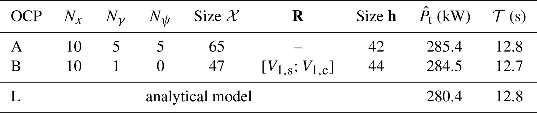
Inequality constraints g, expressed in the time domain, can also be included in the problem (e.g., the minimum elevation angle over the loop can be bounded). A graphical representation of the OCP setup is given in Fig. 2. The derivatives of flight dynamic model with respect to the optimization variables can be taken analytically and provided to the solver, allowing for a deep and fast convergence of the solution. The OCP is implemented in a MATLAB^® environment and solved with the interior-point algorithm implemented in fmincon. As the chosen optimization algorithm (gradient-based) can only look for local optima, the initial guess may influence the solution. In this work, the initial guesses are taken to be circular trajectories, leading to circular-shaped optimal trajectories. Figure-of-eight trajectories can be implemented as initial guesses, which may lead to figure-of-eight-shaped optimal trajectories. A detailed comparison between these two trajectory types is left for future works. The OCPs are solved on an Intel Core i7-9700 3.0 GHz, 16 GB RAM, system. The computation times of the presented examples require from a few seconds to tens of seconds. For example, OCP A in Sect. 6 takes approximately 25 s, and OCP B takes approximately 12 s.

3 Steady-state model

To compare the results of the optimal control problem with idealized analytical expressions, the main results from a refined version of the Loyd power equation (Loyd, 1980) are here briefly recalled. The thrust power equation, with the assumption of linear crosswind motion (Trevisi et al., 2020b), is

$$\begin{array}{}\text{(27)}& \begin{array}{rl}{P}_{\mathrm{t},\mathrm{L}}& ={\displaystyle \frac{\mathrm{1}}{\mathrm{2}}}\mathit{\rho }A{v}_{\mathrm{w}}^{\mathrm{3}}\mathit{\gamma }{\displaystyle \frac{C_{\mathrm{L}}}{G}}{\left(\mathrm{1}+{\left({\displaystyle \frac{G}{\mathrm{1}+\mathit{\gamma }}}\right)}^{\mathrm{2}}\right)}^{\mathrm{3}/\mathrm{2}}\\ & ={\displaystyle \frac{\mathrm{1}}{\mathrm{2}}}\mathit{\rho }A{v}_{\mathrm{w}}^{\mathrm{3}}\mathit{\gamma }{\displaystyle \frac{C_{\mathrm{L}}}{G}}{\left(\mathrm{1}+G_{\mathrm{t}}^{\mathrm{2}}\right)}^{\mathrm{3}/\mathrm{2}},\end{array}\end{array}$$

where the system glide ratio (including tether drag) is $G=\frac{C_{\mathrm{L}}}{C_{\mathrm{D}}}$, and, for readability, a modified glide ratio is defined as $G_{\mathrm{t}}=\frac{C_{\mathrm{L}}}{C_{\mathrm{D}}(\mathrm{1}+\mathit{\gamma })}$ by including the drag of the onboard propellers. The shaft power takes into account the onboard wind turbine induction a:

$$\begin{array}{}\text{(28)}& P_{\mathrm{s},\mathrm{L}}=(\mathrm{1}-a)P_{\mathrm{t},\mathrm{L}}=\left({\displaystyle \frac{\mathrm{1}}{\mathrm{2}}}+{\displaystyle \frac{\mathrm{1}}{\mathrm{2}}}\sqrt{\mathrm{1}-\mathit{\gamma }{C}_{\mathrm{D}}{\displaystyle \frac{A}{A_{\mathrm{t}}}}}\right)P_{\mathrm{t},\mathrm{L}}.\end{array}$$

Finally, the power generated and sent to the grid takes into account the efficiencies of the electrical conversion:

$$\begin{array}{}\text{(29)}& P_{\mathrm{L}}={\mathit{\eta }}_{\mathrm{el}}{P}_{\mathrm{s},\mathrm{L}}.\end{array}$$

For high G, the power equation simplifies to

$$\begin{array}{}\text{(30)}& P_{\mathrm{L}}\approx {\displaystyle \frac{\mathrm{1}}{\mathrm{2}}}\mathit{\rho }A{v}_{\mathrm{w}}^{\mathrm{3}}{C}_{\mathrm{L}}{G}^{\mathrm{2}}{\mathit{\eta }}_{\mathrm{el}}\left({\displaystyle \frac{\mathrm{1}}{\mathrm{2}}}+{\displaystyle \frac{\mathrm{1}}{\mathrm{2}}}\sqrt{\mathrm{1}-\mathit{\gamma }{C}_{\mathrm{D}}{\displaystyle \frac{A}{A_{\mathrm{t}}}}}\right){\displaystyle \frac{\mathit{\gamma }}{(\mathrm{1}+\mathit{\gamma }{)}^{\mathrm{3}}}}.\end{array}$$

For this expression, the value of γ which maximizes the power is only a function of the non-dimensional quantity $C_{\mathrm{D}}\frac{A}{A_{\mathrm{t}}}$. In Fig. 3, the electrical power P_L, normalized with the maximum electrical power at $C_{\mathrm{D}}\frac{A}{A_{\mathrm{t}}}=\mathrm{0}$, is plotted as a function of γ and $C_{\mathrm{D}}\frac{A}{A_{\mathrm{t}}}$. For increasing values of $C_{\mathrm{D}}\frac{A}{A_{\mathrm{t}}}$, the value of γ which maximizes power production decreases. The maximum normalized power as a function of $C_{\mathrm{D}}\frac{A}{A_{\mathrm{t}}}$ is shown in Fig. 4, highlighting that the analytical expression predicts a decrease in power production for increasing $C_{\mathrm{D}}\frac{A}{A_{\mathrm{t}}}$.

Figure 3 Normalized power $\frac{P_{\mathrm{L}}}{P_{\mathrm{L}}(C_{\mathrm{D}}\frac{A}{A_{\mathrm{t}}}=\mathrm{0})}$ as a function of $C_{\mathrm{D}}\frac{A}{A_{\mathrm{t}}}$ for high glide ratios G.

Figure 4 Maximum normalized power $\frac{P_{\mathrm{L}}}{P_{\mathrm{L}}(C_{\mathrm{D}}\frac{A}{A_{\mathrm{t}}}=\mathrm{0})}$ as a function of $C_{\mathrm{D}}\frac{A}{A_{\mathrm{t}}}$ for high glide ratios G.

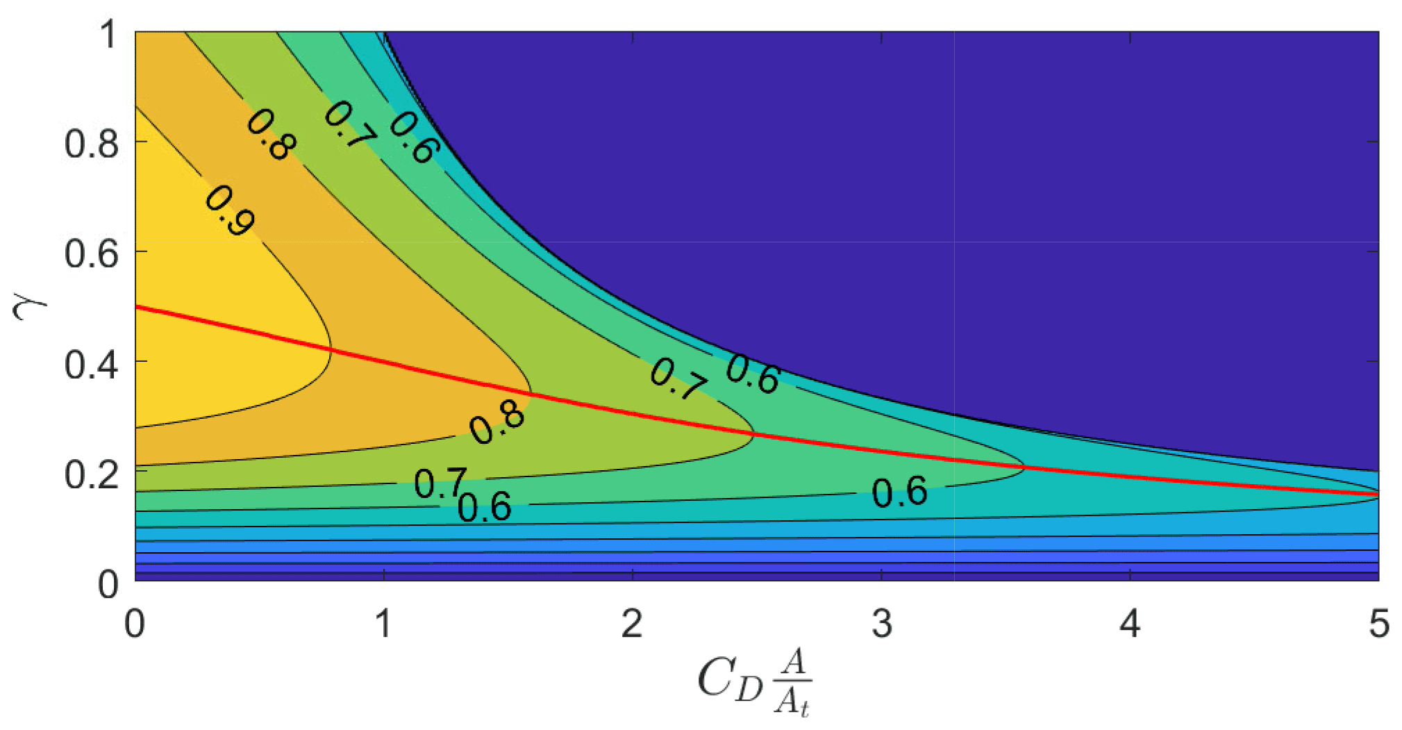
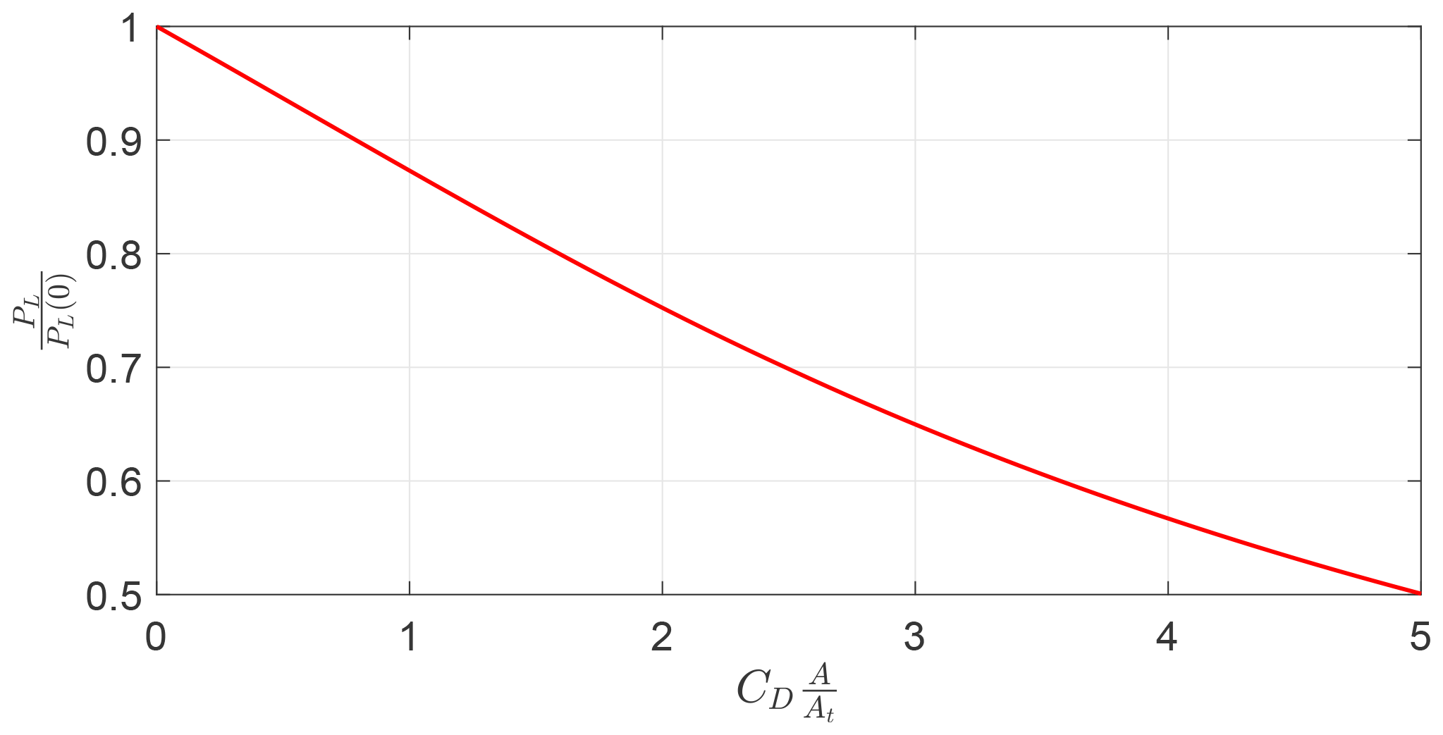
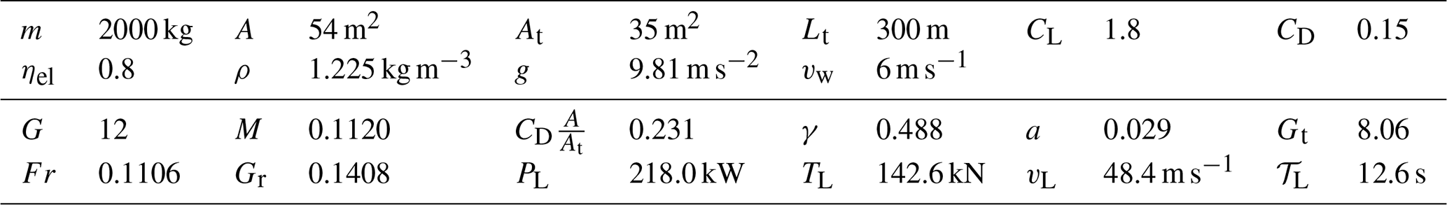
Table 1 Reference values for the examples (values from the Makani MX2 description; Tucker, 2020), associated non-dimensional parameters and quantities evaluated with the steady-state model for γ maximizing Eq. (29).

The tether force can be evaluated as

$$\begin{array}{}\text{(31)}& T_{\mathrm{L}}={\displaystyle \frac{\mathrm{1}}{\mathrm{2}}}\mathit{\rho }A{v}_{\mathrm{w}}^{\mathrm{2}}{\displaystyle \frac{C_{\mathrm{L}}}{G_{\mathrm{t}}}}{\left(\mathrm{1}+G_{\mathrm{t}}^{\mathrm{2}}\right)}^{\mathrm{3}/\mathrm{2}}.\end{array}$$

Trevisi et al. (2020a) showed that for high G, neglecting gravity and with constant incoming wind, there exists an opening angle $\stackrel{\mathrm{̃}}{\mathrm{\Phi }}$ (angle swept by the AWES during the circular trajectory; see Fig. 5) which erases the power losses due to centrifugal forces and that it is only a function of the non-dimensional mass parameter:

$$\begin{array}{}\text{(32)}& M={\displaystyle \frac{m}{\frac{\mathrm{1}}{\mathrm{2}}\mathit{\rho }A{C}_{\mathrm{L}}{L}_{\mathrm{t}}}}.\end{array}$$

In this idealized case, the turning radius is $R=L_{\mathrm{t}}\sin \stackrel{\mathrm{̃}}{\mathrm{\Phi }}$ and the revolution period is

$$\begin{array}{}\text{(33)}& {\mathcal{T}}_{\mathrm{L}}={\displaystyle \frac{\mathrm{2}\mathit{\pi }R}{v_{\mathrm{L}}}}={\displaystyle \frac{\mathrm{2}\mathit{\pi }R}{v_{\mathrm{w}}{G}_{\mathrm{t}}}},\end{array}$$

where v_L is norm of the AWES velocity.

In addition to the non-dimensional mass parameter, the Froude number, which weights the fluid inertial forces to gravity forces, is used in this work:

$$\begin{array}{}\text{(34)}& Fr=\sqrt{{\displaystyle \frac{v_{\mathrm{w}}^{\mathrm{2}}}{g\cdot L_{\mathrm{t}}}}},\end{array}$$

where the reference velocity is the wind velocity and the reference length is the tether length. By combining the previously introduced non-dimensional parameters, the gravity ratio G_r is defined as

$$\begin{array}{}\text{(35)}& G_{\mathrm{r}}={\displaystyle \frac{M}{F{r}^{\mathrm{2}}{G}_{\mathrm{t}}^{\mathrm{2}}}}={\displaystyle \frac{mg}{\frac{\mathrm{1}}{\mathrm{2}}\mathit{\rho }A{C}_{\mathrm{L}}{v}_{\mathrm{w}}^{\mathrm{2}}{G}_{\mathrm{t}}^{\mathrm{2}}}},\end{array}$$

which represents the ratio between gravitational force and aerodynamic lift, similarly to the one introduced in Pasquinelli (2021).

In the following sections, the results will be generalized as a function of the non-dimensional parameters just introduced. Input parameters from the Makani MX2 design (Tucker, 2020) will be used as reference values to present the results (Table 1).

4 Validation of the frequency-domain formulation against time integration

To make sure the frequency-domain formulation is well implemented and finds solutions which respect the equations of motion, they are compared with the solution coming from a time integration scheme. The model described in Sect. 2.1 is solved with the MATLAB^® ode45 integration scheme. After solving the periodic solution with the harmonic balance methodology, the Fourier coefficients of the state and control vector are retrieved. The state vector at t=0 is used as an initial condition for the numerical integration. The control inputs must be computed from their Fourier series at every step of the integration. In Appendix B, a comparison for a circular and a figure-of-eight trajectory is shown. The solution of the dynamics, represented by the azimuth and elevation, for the two cases is equivalent, demonstrating that the frequency-domain formulation is accurate enough to be used in the present optimal control problem framework.

5 Optimal control problems with constant inflow and no elevation angle constraints

As the analysis is limited to circular trajectories, a cylindrical reference frame ℱ_C, similar to the one employed in Trevisi et al. (2020a, 2021) and Pasquinelli (2021), is used to present the results. A graphical representation of ℱ_C is given in Fig. 5. The longitudinal axis of ℱ_C is aligned with the mean elevation angle $\widehat{\mathit{\beta }}$. The angle β_m denotes the minimum elevation angle and Φ the opening angle. The angular position of the AWES is defined by α, and when α=0 the AWES moves upward (i.e., $\dot{\mathit{\alpha }}>\mathrm{0}$).

Figure 5 Cylindrical reference system ℱ_C used to analyze circular trajectories.

To increase complexity incrementally, the optimal control problems (OCPs) are modified from the most idealized case to a realistic one. For the idealized cases analyzed in this section, uniform incoming wind speed (α_s=0) and no minimum elevation angle constraints are considered. In this section, β_s (Eq. 5) is set equal to zero, such that e₃ points upwind. In this way, when the roll is equal to zero (ψ=0^∘), the span direction is perpendicular to the incoming wind.

5.1 Optimizing for the mean electrical power in the absence of gravity

For the most idealized case, the gravity is null g=0, such that Fr→∞ and G_r=0. The objective function is taken as the mean electrical power, given in Eq. (15). By solving the OCP for the example (Table 1), it is found that the solution has constant values over the trajectory and the average power output is equal to the one evaluated with the analytical expression in Eq. (29). Figure 6 shows the evolution of β and ϕ, highlighting that the solution is a circle. Due to the constant values of the solution, quantities such as tether force along the axial symmetry axis, γ, AWES velocity and others can be found with the formulation assuming a crosswind straight motion, as Sect. 3.

Figure 6 Optimal trajectory.

For the solution to be optimal, it is found that the AWES span is perpendicular to the wind speed, or, in analytical terms, that ψ=0. Figure 7 shows the optimal opening angle Φ^* as a function of a modified non-dimensional mass parameter M_t found by solving a number of OCPs with different G (G∈[10 30]), M (M∈[0.025 0.15]) and $C_{\mathrm{D}}\frac{A}{A_{\mathrm{t}}}$ ($C_{\mathrm{D}}\frac{A}{A_{\mathrm{t}}}\in \left[\mathrm{0}\mathrm{0.4}\right]$).

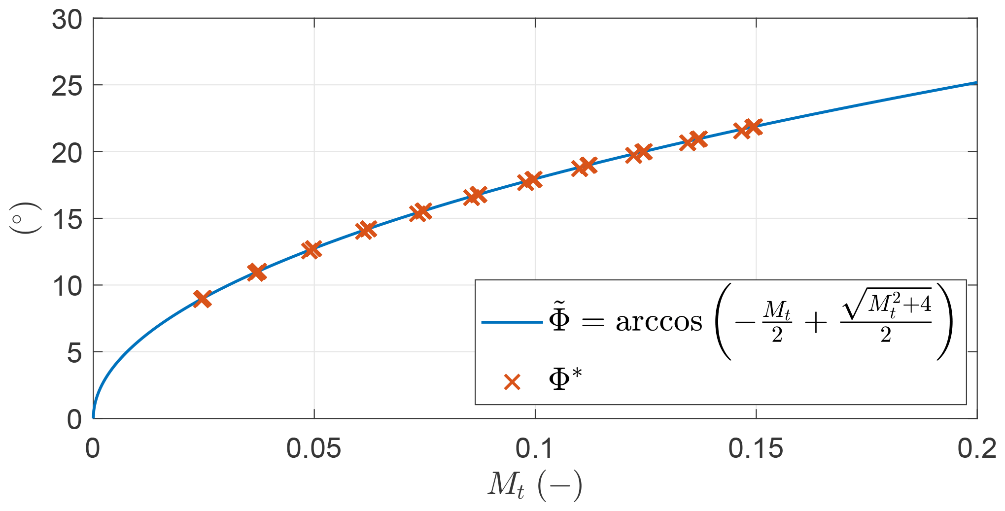
Figure 7 Optimal opening angles Φ^* (x) found by solving multiple OCPs and analytical expression (–) as a function of the modified non-dimensional mass parameter M_t.

The values of Φ^* can be accurately described by

$$\begin{array}{}\text{(36)}& \stackrel{\mathrm{̃}}{\mathrm{\Phi }}=\arccos \left(-{\displaystyle \frac{M_{\mathrm{t}}}{\mathrm{2}}}+{\displaystyle \frac{\sqrt{M_{\mathrm{t}}^{\mathrm{2}}+\mathrm{4}}}{\mathrm{2}}}\right),M_{\mathrm{t}}={\displaystyle \frac{M}{\mathrm{1}+\frac{\mathrm{1}}{G_{\mathrm{t}}^{\mathrm{2}}}}},\end{array}$$

which for high glide ratios coincides with the analytical formulation given in Trevisi et al. (2020a).

Table 2 Settings of the two optimal control problems maximizing the mean thrust power considering gravity. V_1,s and V_1,c are the first Fourier coefficients of the norm of the AWES velocity v.

5.2 Optimizing for the mean thrust power considering gravity

Gravity is now included in the modeling, and the objective function is taken as the mean thrust power ${\widehat{P}}_{\mathrm{t}}$ (Eq. 12). The results of two slightly different OCPs are shown for the sake of understanding the results, and they are summarized in Table 2. In OCP A, the control inputs are modeled with five harmonics. In OCP B, the time series of the control input ψ is modeled as a constant, and only one harmonic is used for the control input γ. Additionally, the norm of the AWES velocity $v=\left|\mathit{v}\right|$ is imposed to be constant (additional equality constraint). As the control inputs act up to the first harmonic, this constraint is set by imposing the first Fourier coefficients of the AWES velocity to zero ($\mathbf{R}=[V_{\mathrm{1},\mathrm{s}};V_{\mathrm{1},\mathrm{c}}]$), while no constraints are imposed on the higher-order harmonics. In Table 2, the mean thrust power (objective function) is also reported and compared with the analytical formulation (Eq. 27). The objective function of the two OCPs is almost the same, showing that the two problems are basically equivalent.

By solving the OCPs, it is found that the optimal solutions have a negative mean elevation of ${\widehat{\mathit{\beta }}}_A\approx -\mathrm{8.2}$^∘ and ${\widehat{\mathit{\beta }}}_B\approx -\mathrm{7.8}$^∘. The trajectories, shown in Fig. 8, have a circular shape (a circle with radius $\stackrel{\mathrm{̃}}{\mathrm{\Phi }}$ is marked as $-.$), but it is no longer a perfect circle.

Figure 8 Optimal trajectory for OCP A (−), B ($--$) and a circle with radius $\stackrel{\mathrm{̃}}{\mathrm{\Phi }}$ ($-.$).

Figure 9 Optimal ψ as a function of the angular position.

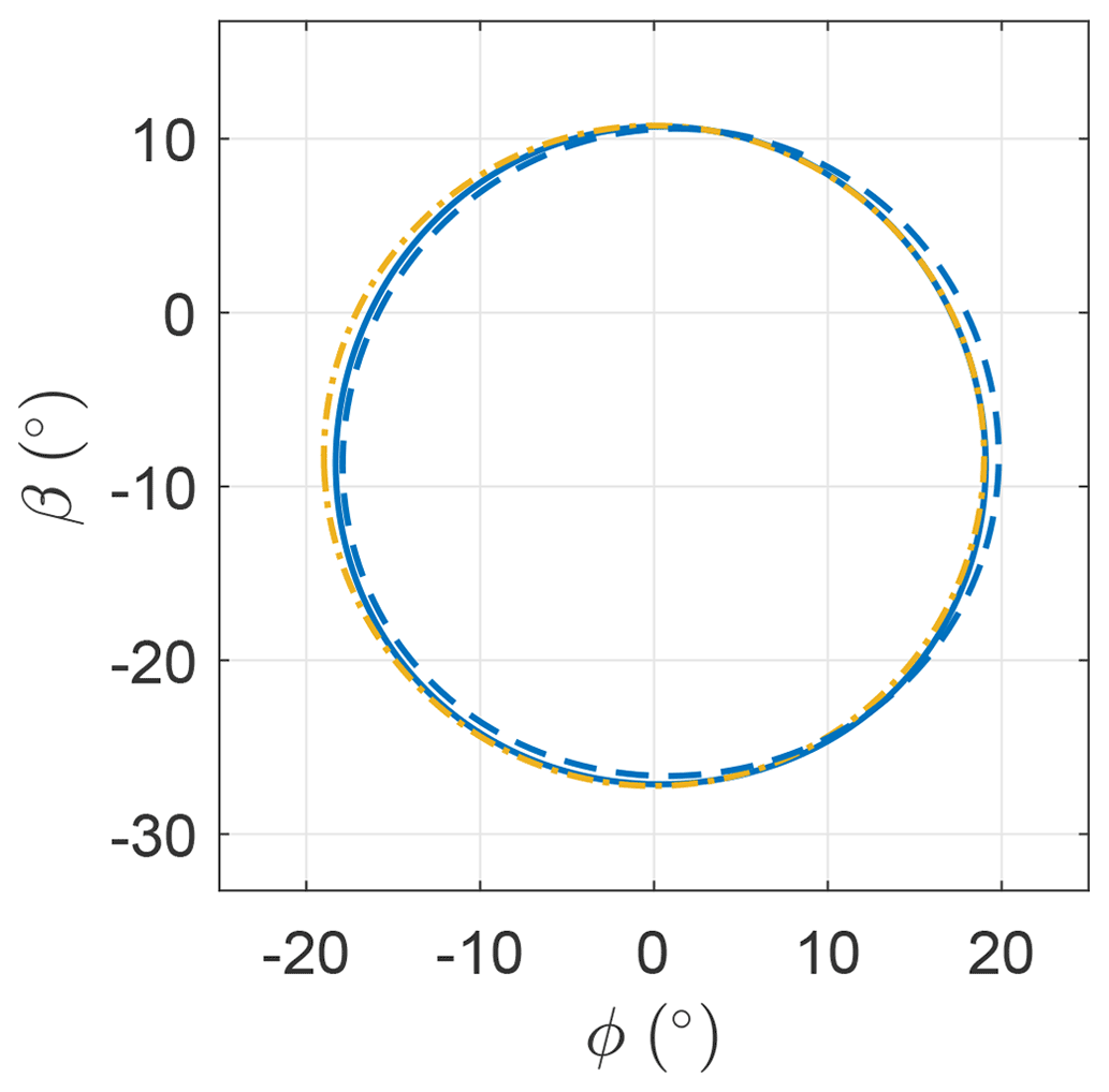
Figure 9 shows the trends of the control input ψ as a function of α (see Fig. 5 for definition). For OCP A, it fluctuates with small amplitude about the mean value, which is close to zero. For this reason, it is modeled as a constant in OCP B. The optimal constant value is also close to zero, meaning that the AWES span is perpendicular to the wind speed direction. Since the two OCPs present similar optimal values of power, it is found that the optimal solutions are not sensitive to the fluctuations of the roll angle ψ.

Figure 10 shows the evolution of γ as a function of α. The mean values for the two OCPs are close to the value maximizing Eq. (27), denoted in figure as γ_L. γ takes values higher than the mean in the descending leg of the loop and negative values in the ascendant leg. This means that in the ascendant leg the onboard wind turbines are operated as propellers. In OCP A γ is modeled with five harmonics, while in OCP B it is modeled with just one. As the objective function of the two optimal solutions is similar, it is found that the trend of γ can be modeled with just one harmonic.

Figure 10 Optimal γ as a function of the angular position.

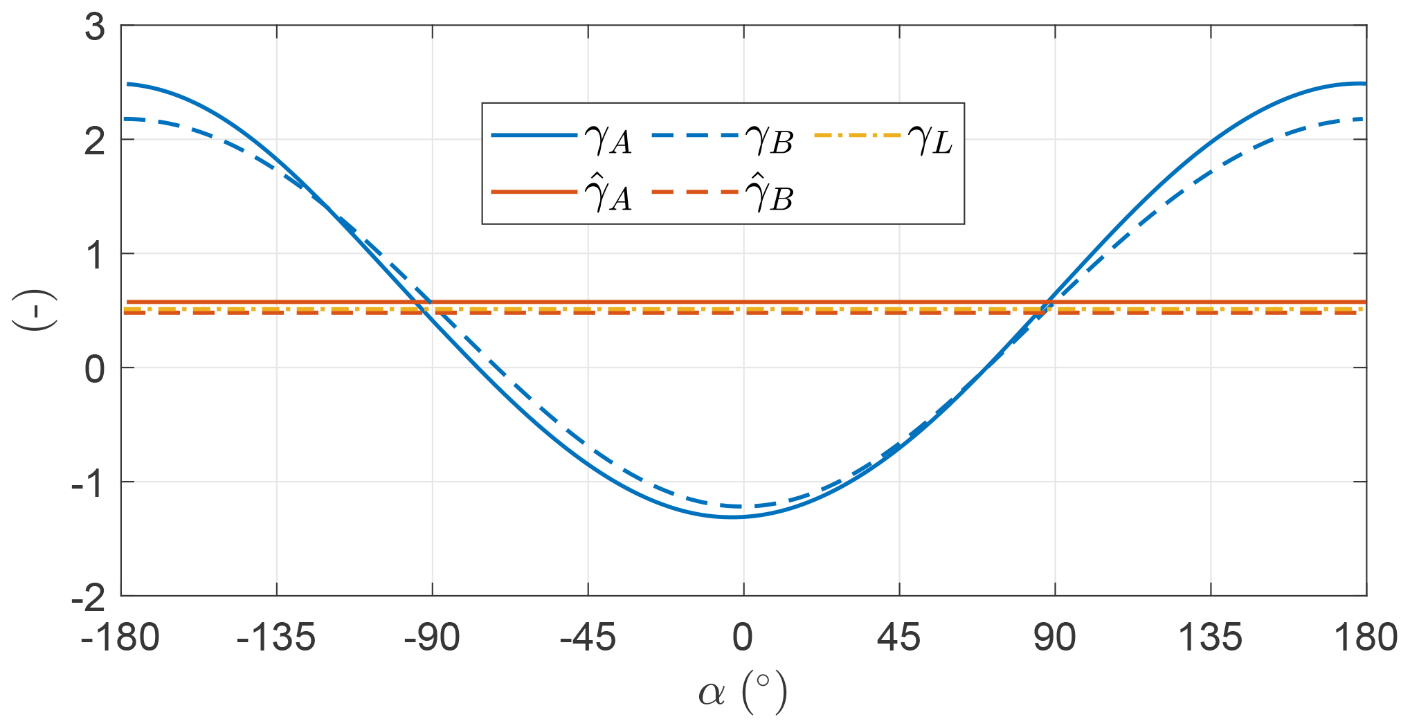
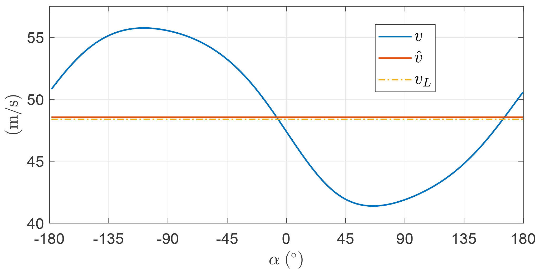
Figure 11 shows the norm of the optimal AWES velocity v for the two OCPs. In OCP B, this value is constrained to be a constant by imposing only its first harmonic null. Since it is not possible to impose constraints at frequencies where the control (γ and ψ) is not acting, higher-order harmonics are not constrained. The mean values of v are similar the one predicted by the steady model. Since the fluctuations for OCP A are small compared to the mean, the influence of the velocity fluctuations on the overall performances is investigated in OCP B, showing that they impact weakly the optimal solution. As the two OCPs are basically equivalent, it is found that optimal trajectories are characterized by a AWES constant velocity.

Figure 11 Norm of the optimal AWES velocity v as a function of the angular position.

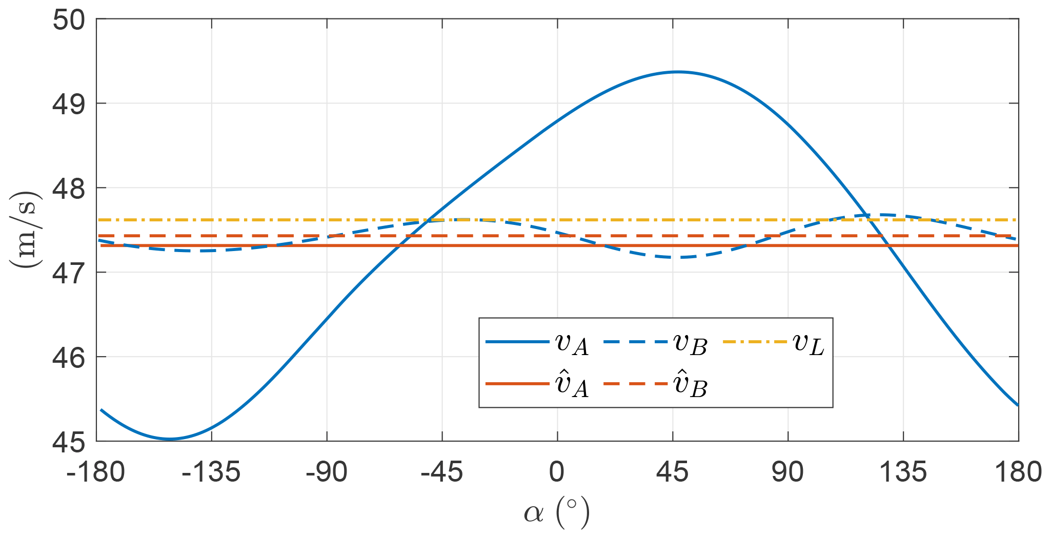
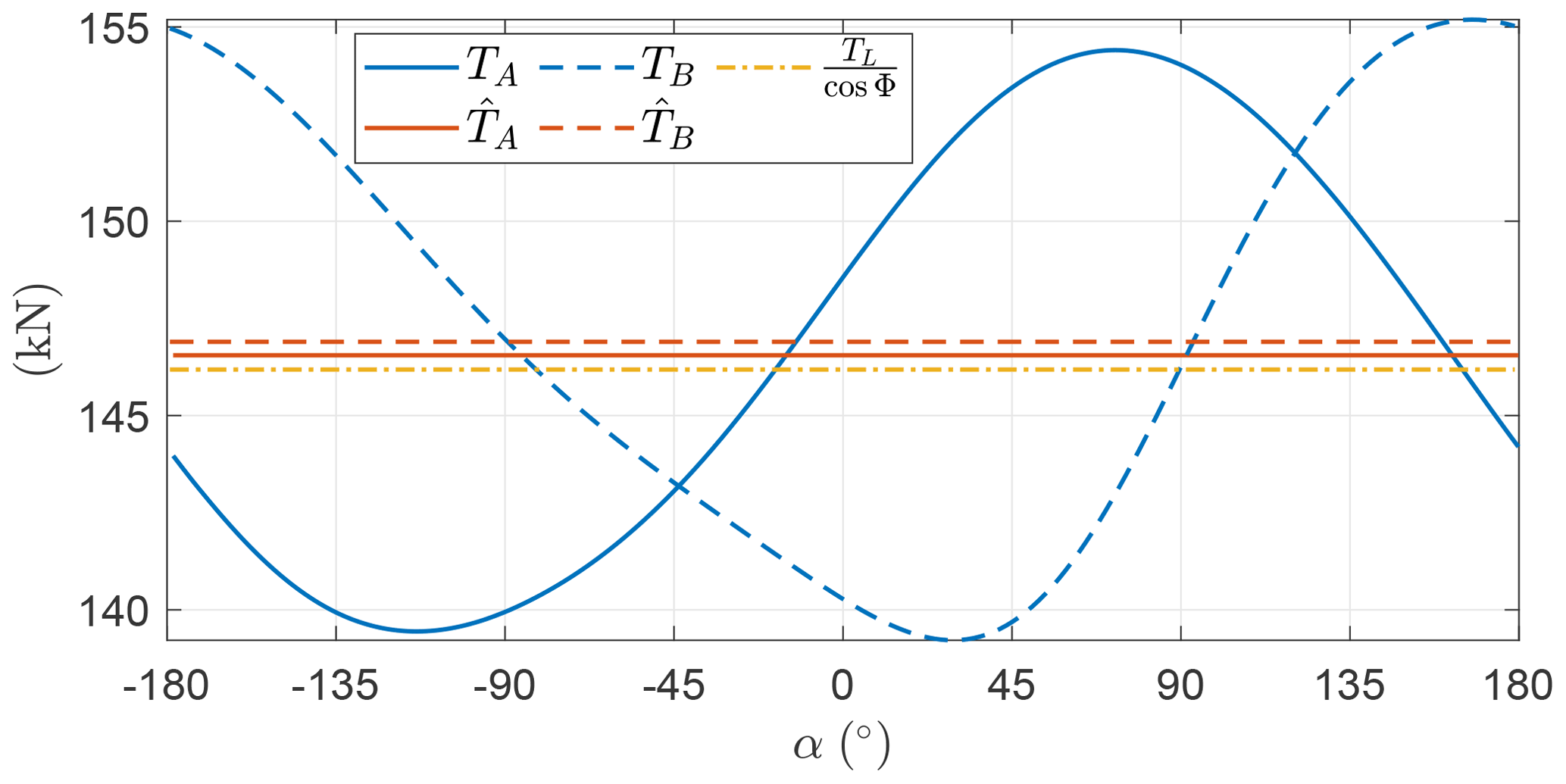
Figure 12 shows the magnitude of the tether force for the two cases. As it scales with the relative wind speed squared, also the tether force has an almost constant trend (the fluctuations are small compared to the mean).

Figure 12 Tether force T as a function of the angular position.

To compare the two OCPs and draw some conclusions, the power output, shown in Fig. 13, is to be analyzed. The mean thrust power output for the two OCPs is slightly higher than P_t,L. This is due to a nonlinear effect induced by the combination of gravity and mean elevation angle different from zero as compared to the idealized case. Indeed, for negative mean elevation, the combination leads to an increase of mean thrust power, while the opposite occurs in case of positive mean elevation. As the effects on power is almost negligible and it does not primarily impact the main outcomes of this paper, a detailed explanation of this phenomenon is avoided here, but the reader can find more details in Pasquinelli (2021). The theoretical thrust power, given in Eq. (27), is derived neglecting gravity. However, it approximates well the power output obtained through the OCP, which includes gravity.

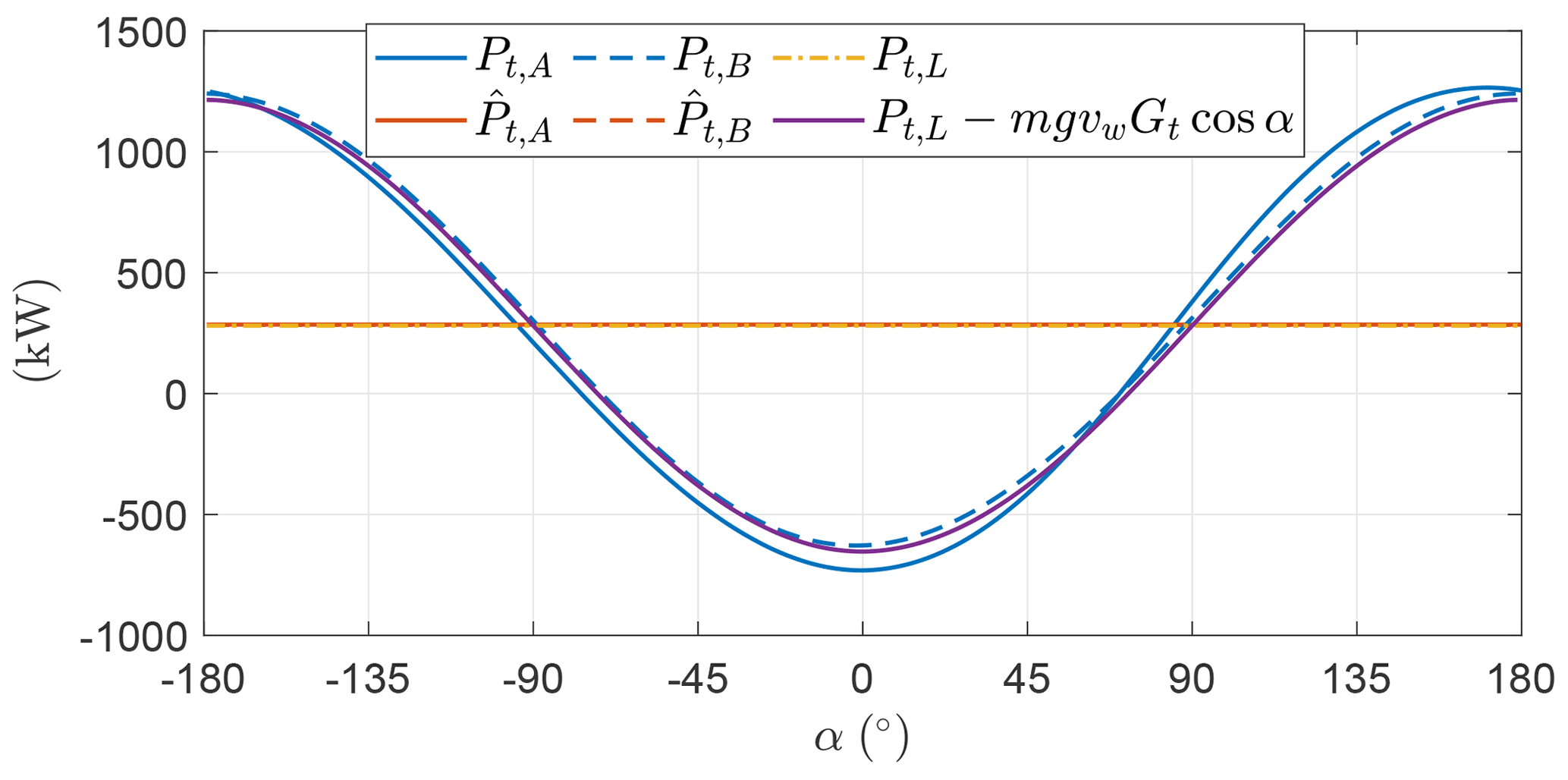
Figure 13 Optimal thrust power production and consumption P_t as a function of the angular position.

As the two analyzed OCPs are almost equivalent, the optimal trajectories are characterized by the perpendicularity of the AWES span with respect to the wind (ψ=0) and a constant AWES velocity. In order to keep the AWES velocity constant over the loop, the onboard wind turbines balance the action of the gravitational force. In the descendent leg, the onboard wind turbines harvest the gravitational potential energy, and in the ascendant leg, that power is given back to the system.

Following these considerations, the power trend, as shown in Fig. 13, can then be approximated as

$$\begin{array}{}\text{(37)}& P_{\mathrm{t}}\left(\mathit{\alpha }\right)\approx P_{\mathrm{t},\mathrm{L}}+{\mathit{F}}_{\mathrm{g}}\cdot \mathit{v}\approx P_{\mathrm{t},\mathrm{L}}-mg{v}_{\mathrm{w}}{G}_{\mathrm{t}}\cos \mathit{\alpha }.\end{array}$$

The onboard wind turbine thrust can be approximated with ${\mathit{D}}_{\mathrm{t}}\approx (\widehat{\mathit{\gamma }}+A_{\mathit{\gamma },\mathrm{1}}\cos (\mathit{\alpha }-{\mathit{\theta }}_{\mathit{\gamma },\mathrm{1}}\left)\right)\mathit{D}$, where D is constant because the AWES velocity is found to be constant, and from Fig. 10 it is found that ${\mathit{\theta }}_{\mathit{\gamma },\mathrm{1}}\approx \mathrm{180}$^∘. As the thrust power can be written as the product of D_t and the relative wind speed v_r (Eq. 12), the amplitude of the first Fourier coefficient of γ, considering Eq. (37), can be approximated by

$$\begin{array}{}\text{(38)}& A_{\mathit{\gamma },\mathrm{1}}\approx {\displaystyle \frac{{\mathit{F}}_{\mathrm{g}}\cdot \mathit{v}}{-\cos \mathit{\alpha }\mathit{D}\cdot {\mathit{v}}_{\mathrm{r}}}}\approx {\displaystyle \frac{mg}{\frac{\mathrm{1}}{\mathrm{2}}\mathit{\rho }A{C}_{\mathrm{D}}{v}_{\mathrm{w}}^{\mathrm{2}}{G}_{\mathrm{t}}^{\mathrm{2}}}}=G_{\mathrm{r}}G.\end{array}$$

Figure 14 shows the comparison of A_γ,1 found numerically by running the OCP (with the settings of OCP B) for a different combination of M (M∈[0.025 0.15]), G (G∈[10 30]), and Fr (Fr∈[0.1 0.2]) and the analytical approximation given in Eq. (38).

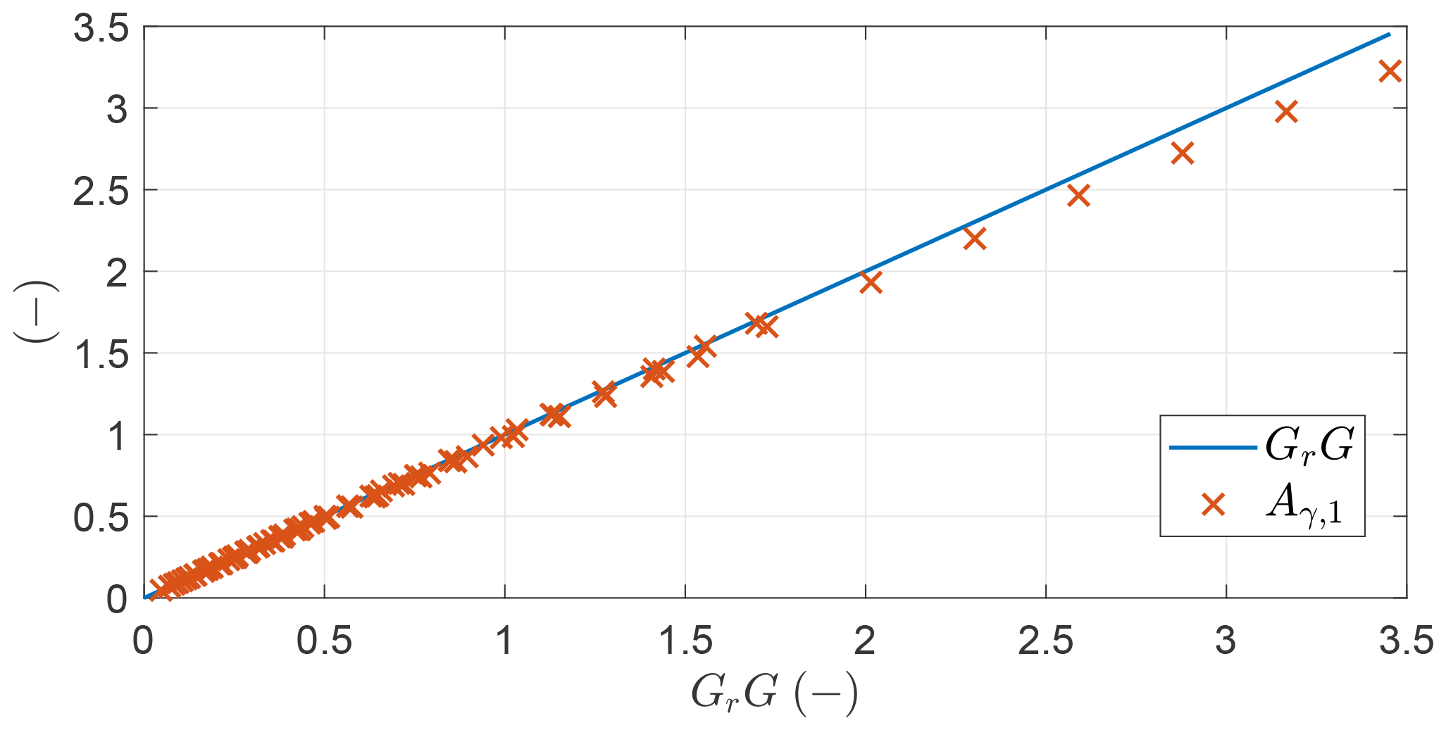
Figure 14 Amplitude of the first Fourier coefficient of γ (x) found by solving multiple OCPs and analytical approximation (–) as a function of G_rG.

Figure 15 shows the first Fourier coefficient of elevation β and azimuth ϕ as a function of the non-dimensional parameter M_t, as they represent the width and height of the trajectory. The analytical expression given in Eq. (36) is still a good approximation of the optimal trajectory shape.

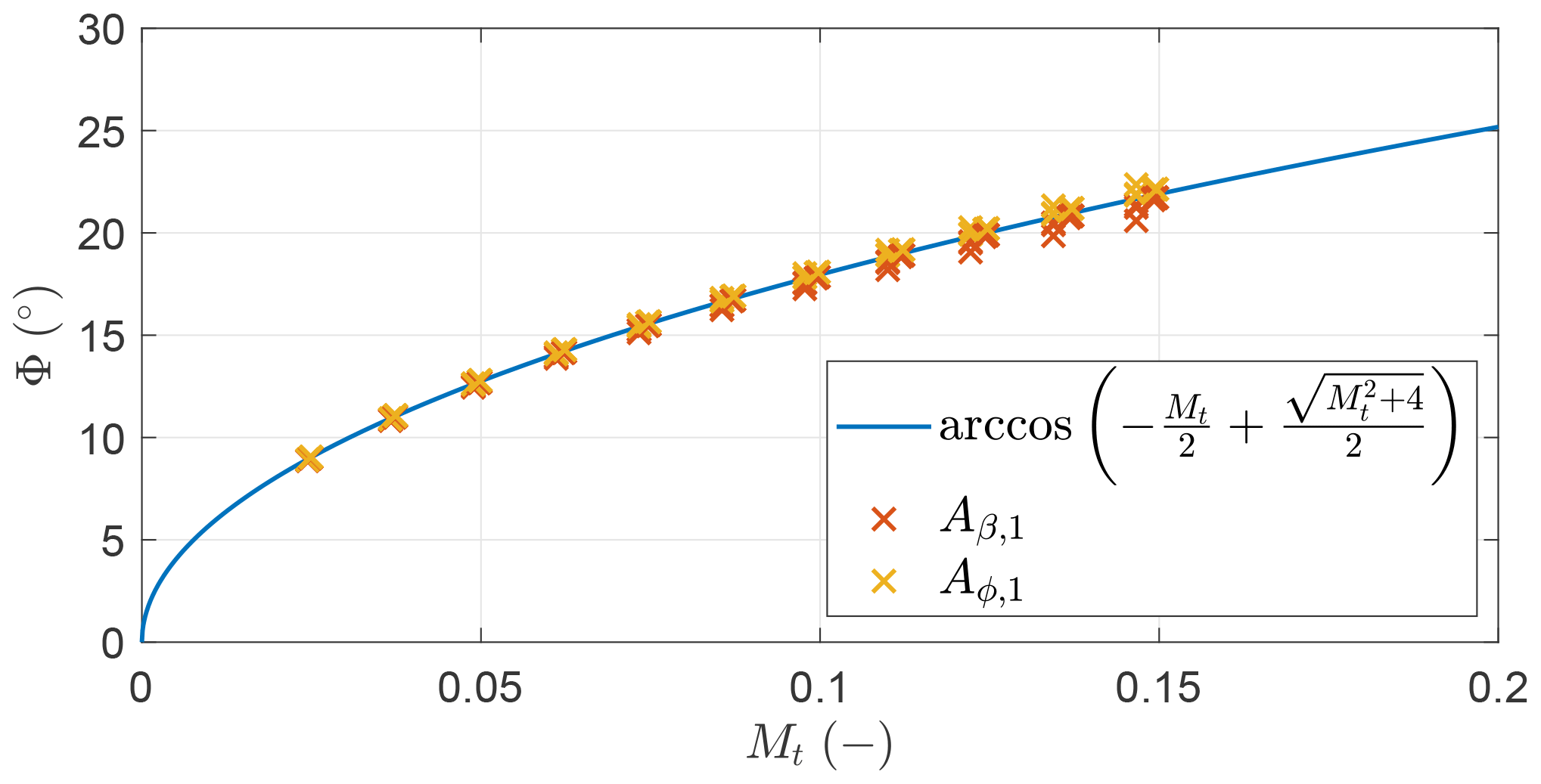
Figure 15 First Fourier coefficient of elevation β and azimuth ϕ (x) found by solving multiple OCPs and analytical expression (–) as a function of the modified non-dimensional mass parameter M_t.

5.3 Optimizing for the mean shaft power considering gravity

In this section, the onboard wind turbine induction is included in the power evaluation, and the mean shaft power ${\widehat{P}}_{\mathrm{s}}$ is considered as objective function. To present the results, two different OCPs are introduced (Table 3). The mean shaft power for OCP A and B is almost identical, highlighting that one harmonic to model the productive drag and two for the roll are enough. The power for the analytical case is found by maximizing Eq. (28) with respect to γ. The figures in this section refer to OCP B.

Table 3 Settings of the two optimal control problems maximizing the mean shaft power considering gravity.

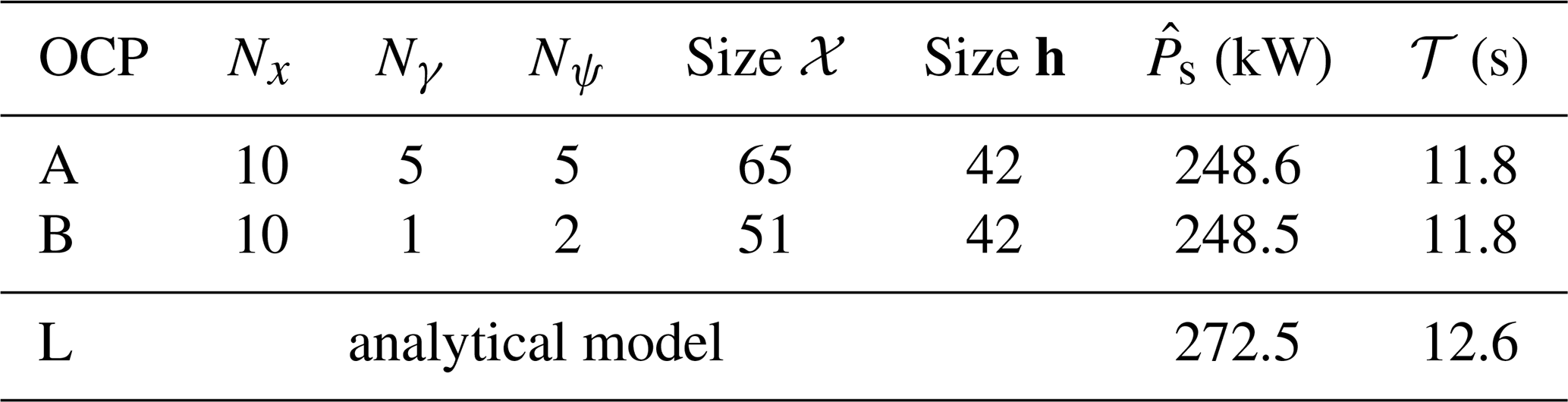
Figure 16 shows the trajectory in the β–ϕ plane. The trajectory deviates from a circular shape, especially along the β axis, and has a mean elevation angle of ${\widehat{\mathit{\beta }}}_B=-\mathrm{5.5}$^∘, higher than for the case without induction.

Figure 16 Optimal trajectory (–) and a circle with radius $\stackrel{\mathrm{̃}}{\mathrm{\Phi }}$.

Figure 17 shows the roll angle as a function of the angular position in the loop. Even in this case with induction, the fluctuations are relatively small. When the AWES increases the turning radius (approximately between $-\mathrm{90}{}^{\circ }<\mathit{\alpha }<\mathrm{0}{}^{\circ }$ and $\mathrm{90}{}^{\circ }<\mathit{\alpha }<-\mathrm{180}{}^{\circ }$; see Fig. 16), the roll decreases.

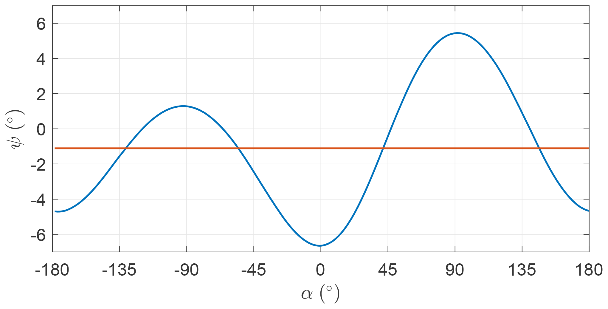
Figure 17 Optimal ψ (blue line) and its mean (red line) as a function of the angular position.

Figure 18 Optimal γ as a function of the angular position.

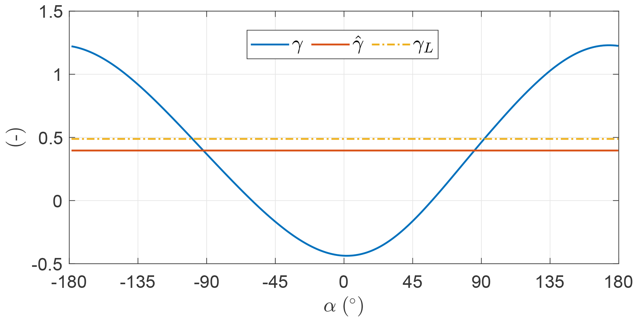
Figure 18 shows γ as a function of the angular position. The mean value is smaller compared to the value maximizing Eq. (28). By comparing the trends with Fig. 10, it is clear that the fluctuations of γ are lower than in the case without induction. The onboard wind turbine induction a has a similar trend to γ, as a and γ are linked through the expression in Eq. (28). When γ takes negative values – in the ascendant leg – the onboard wind turbines are operated as propellers and the induction is negative. In the descendent leg, γ takes values larger than the mean and so does the induction. Higher values of induction result in a lower ratio between shaft power, which is the power the optimizer maximizes, and thrust power, which is the power directly linked to the dynamics. Therefore, high values of γ are not beneficial for the shaft power production.

In Fig. 19, the AWES velocity is shown, highlighting that it fluctuates over the loop. When maximizing the mean thrust power (Sect. 5.2), the optimal AWES velocity over the loop was found to be constant. Here, it is optimal to convert part of the potential energy into electrical energy and part into kinetic energy, letting the velocity fluctuate over the loop.

Figure 19 Norm of the optimal AWES velocity v as a function of the angular position.

To conclude the analysis of the example, Fig. 20 shows the shaft and the thrust power. As anticipated, when γ takes higher values than the mean, the induction grows and the ratio between shaft and thrust power decreases consequently.

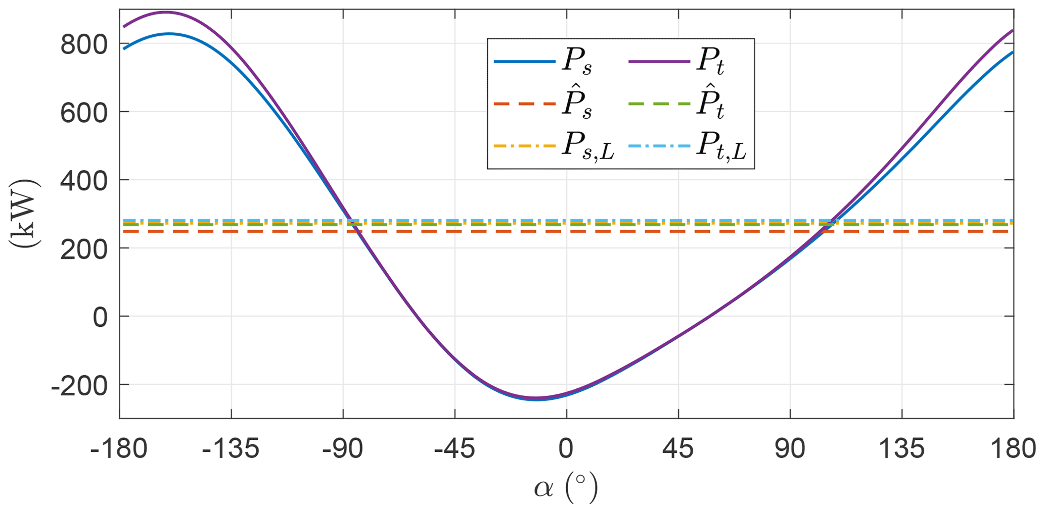
Figure 20 Optimal shaft power production and consumption P_s and thrust power P_t as a function of the angular position.

In Fig. 4 the dependence of the analytical expression of the shaft power on $C_{\mathrm{D}}\frac{A}{A_{\mathrm{t}}}$ is shown. In Fig. 21, the dependence of the optimal mean shaft power is analyzed as a function of the same non-dimensional coefficient for three different Froude numbers (i.e., three wind speeds). In the current example, Fr=0.1 corresponds to v_w=5.4 m s⁻¹, Fr=0.15 corresponds to v_w=8.1 m s⁻¹ and Fr=0.2 corresponds to v_w=10.8 m s⁻¹. For increasing Froude number, the solution gets closer to the analytical formulation because the power fluctuations gradually lose impact on the mean power production. Indeed, the aerodynamic forces become dominant with respect to the gravitational force.

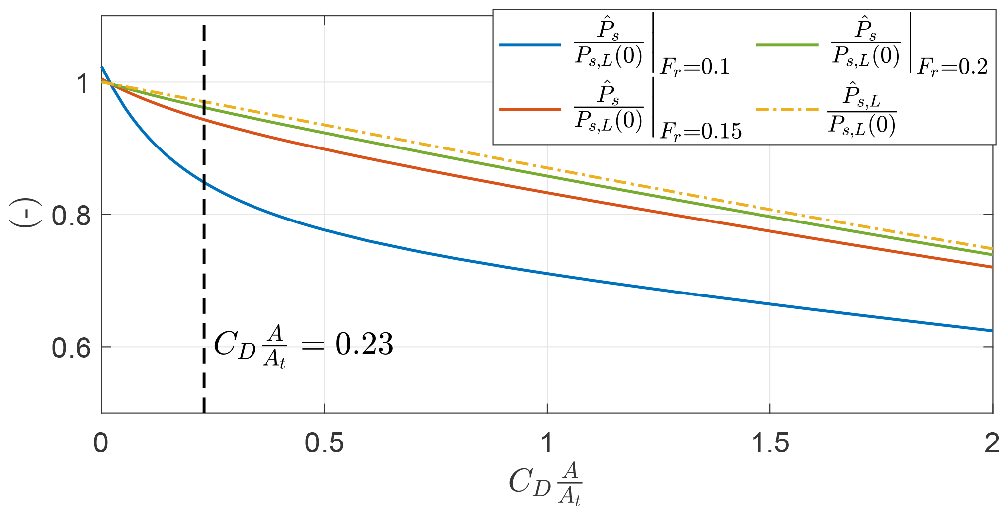
Figure 21 Optimal shaft power production normalized with the analytical expression of thrust power as a function of $C_{\mathrm{D}}\frac{A}{A_{\mathrm{t}}}$.

Figure 22 Optimal values of $\widehat{\mathit{\gamma }}$ and A_γ,1, normalized with G_rG as a function of $C_{\mathrm{D}}\frac{A}{A_{\mathrm{t}}}$ for different Froude numbers.

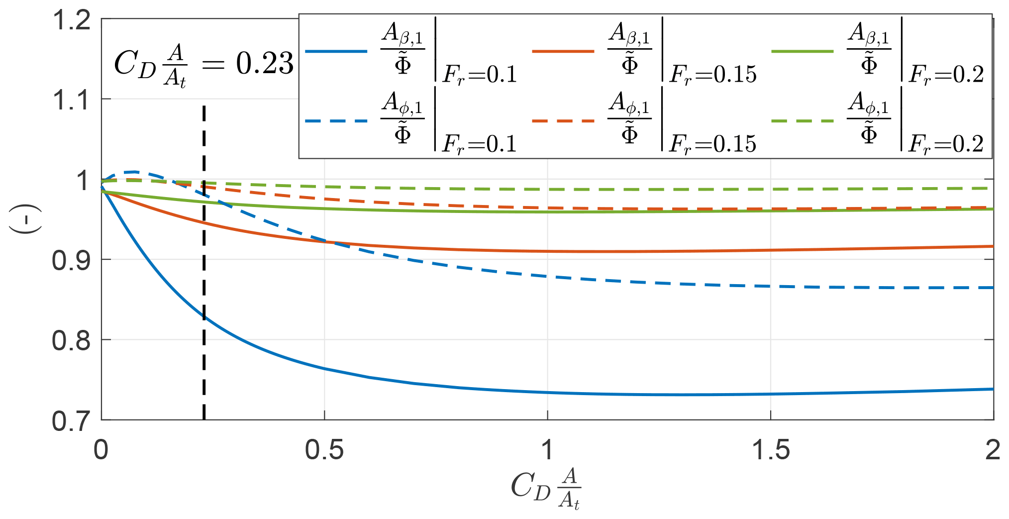
Figure 23 Optimal values of A_β,1 and A_ϕ,1, normalized with the analytical expression of the opening angle $\stackrel{\mathrm{̃}}{\mathrm{\Phi }}$, as a function of $C_{\mathrm{D}}\frac{A}{A_{\mathrm{t}}}$ for different Froude numbers.

In Sect. 5.2, it was found that the amplitude of the first Fourier coefficient of γ for $C_{\mathrm{D}}\frac{A}{A_{\mathrm{t}}}=\mathrm{0}$ (i.e., optimizing for the thrust power) can be approximated by $A_{\mathit{\gamma },\mathrm{1}}\approx G_{\mathrm{r}}G$. In Fig. 22, the trends of $\frac{A_{\mathit{\gamma },\mathrm{1}}}{G_{\mathrm{r}}G}$, with γ being modeled with a single harmonic, for the three investigated Froude numbers, are shown as a function of $C_{\mathrm{D}}\frac{A}{A_{\mathrm{t}}}$. For $C_{\mathrm{D}}\frac{A}{A_{\mathrm{t}}}\to \mathrm{0}$, trends are close to 1. For increasing Fr, the curves collapse to a unique curve. In particular, at $C_{\mathrm{D}}\frac{A}{A_{\mathrm{t}}}=\mathrm{0.23}$, which is the value for the example, the ratio $\frac{A_{\mathit{\gamma },\mathrm{1}}}{G_{\mathrm{r}}G}\to \mathrm{0.54}$ for increasing Fr. For increasing values of $C_{\mathrm{D}}\frac{A}{A_{\mathrm{t}}}$, the ratio $\frac{A_{\mathit{\gamma },\mathrm{1}}}{G_{\mathrm{r}}G}$ tends to zero, highlighting the fact that a less fluctuating value of γ over the loop is beneficial. The plot shows also the value of $\widehat{\mathit{\gamma }}$ as a function of $C_{\mathrm{D}}\frac{A}{A_{\mathrm{t}}}$, highlighting that for increasing Fr the trends collapse to the value maximizing Eq. (28), indicated as γ_L.

Finally, Fig. 23 shows the ratio of the first Fourier coefficient of the elevation angle β and the azimuth angle ϕ with the opening angle $\stackrel{\mathrm{̃}}{\mathrm{\Phi }}$ evaluated with Eq. (36). For $C_{\mathrm{D}}\frac{A}{A_{\mathrm{t}}}\to \mathrm{0}$, values are close to 1, as noted in Fig. 15. As $C_{\mathrm{D}}\frac{A}{A_{\mathrm{t}}}$ increases, the values of A_β,1 decrease more than A_ϕ,1, showing that the optimal trajectory no longer has a circular shape and the height decreases more than the width. This effect is visible also in the example in Fig. 16. At low Froude numbers (i.e., low wind speeds) this effect is more evident.

5.4 Optimizing for the mean electrical power considering gravity

In this section, the electrical efficiency is included into the optimal control problem, and the mean electrical power is considered as objective function. Two OCPs, whose characteristics are given in Table 4, are introduced to present results. The power for OCP A and B is almost identical, highlighting that one harmonic to model the productive drag and two for the roll are enough. The power for the analytical case is found by maximizing Eq. (29) with respect to γ.

Table 4 Settings of the two optimal control problems maximizing the mean electrical power considering gravity.

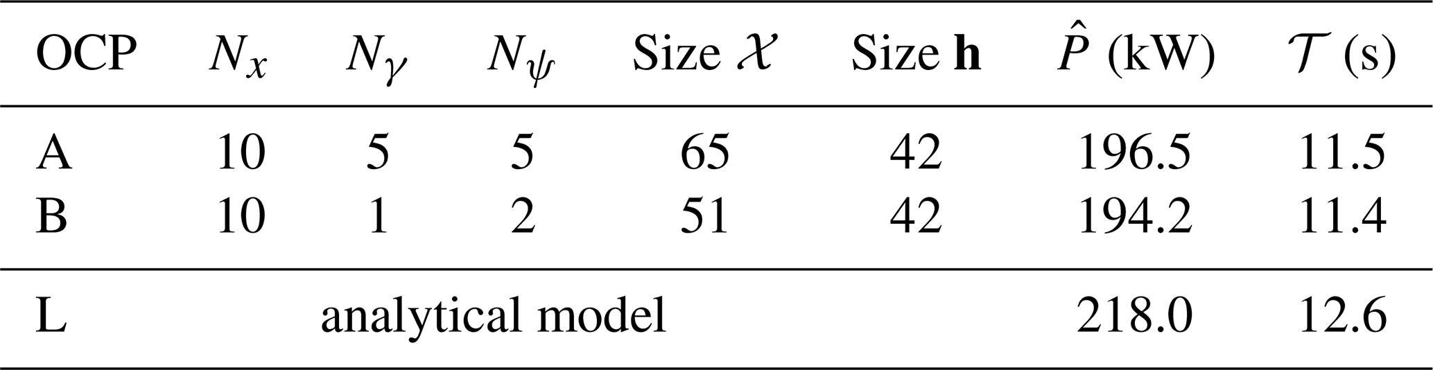
Figure 24 shows the trajectory in the β–ϕ plane. The trajectories deviate from the circular trajectory with opening angle $\stackrel{\mathrm{̃}}{\mathrm{\Phi }}$ (Eq. 36), especially along the β axis, and have a mean elevation angle of ${\widehat{\mathit{\beta }}}_A=-\mathrm{5.1}$^∘ and ${\widehat{\mathit{\beta }}}_B=-\mathrm{4.9}$^∘.

Figure 24 Optimal trajectory for OCP A (−), B ($--$) and a circle with radius $\stackrel{\mathrm{̃}}{\mathrm{\Phi }}$ ($-.$).

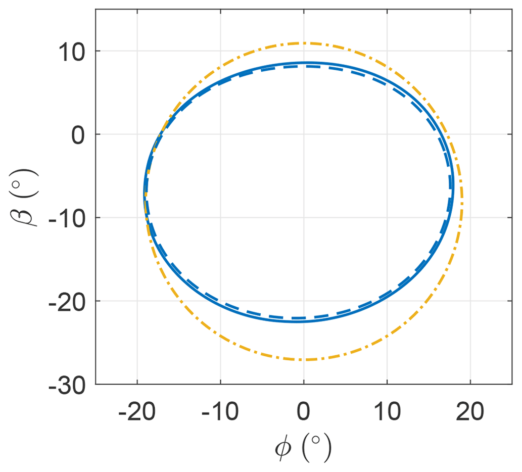
Figure 25 shows the roll angle as a function of the angular position in the loop. As in the case maximizing mean shaft power, the fluctuations are relatively small.

Figure 25 Optimal ψ as a function of the angular position.

Figure 26 Optimal γ as a function of the angular position.

Figure 27 Norm of the optimal AWES velocity v as a function of the angular position.

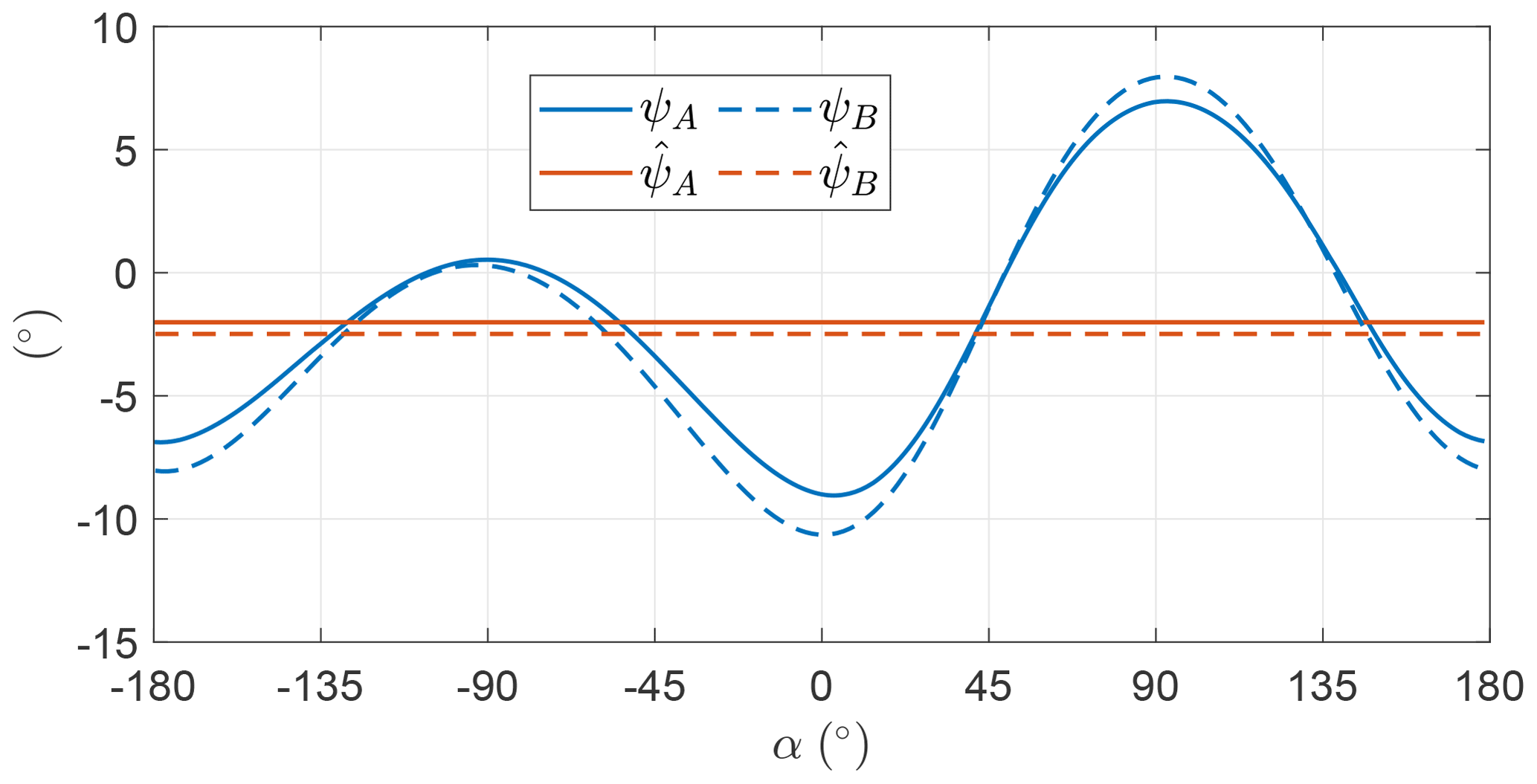
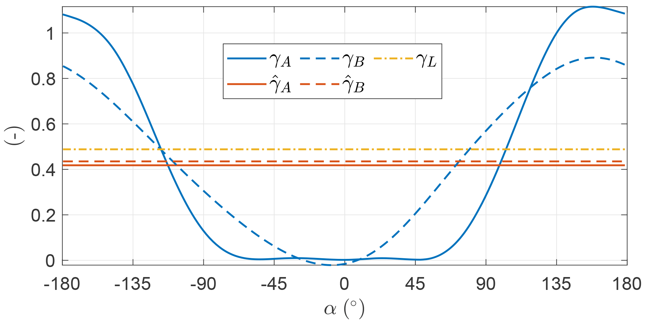
Figure 26 shows γ as a function of the angular position. In OCP A, the time evolution of γ is modeled with five harmonics. In the ascendant leg, γ takes null values, meaning that the power is neither spent nor consumed. Indeed, spending power drastically reduces the overall power production because of the conversion efficiency from electrical to thrust power. This is also highlighted by Tucker (2020). In OCP B, the time evolution of γ is modeled with just one harmonic. The trend is, however, similar to OCP A, with the minimum value being slightly negative. This means that A_γ,1 is similar to $\widehat{\mathit{\gamma }}$.

Figure 27 shows the norm of the AWES velocity over the loop, showing that the trend is similar for the two OCPs, and, as noted in Sect. 5.3, it is optimal to convert part of the potential energy into electrical energy and part into kinetic energy.

The electrical power as a function of the angular position is shown in Fig. 28. As expected when analyzing the trend of γ, the electrical power is null in the ascendant leg and larger than the mean in the descending part. In OCP B, the mean power is slightly lower than in OCP A but the power fluctuations are lower, which could be beneficial from a grid and power smoothing perspective. Due to the electrical efficiency, the wind turbines are not used as propellers anymore. This results in an even more squashed trajectory (Fig. 24) with respect to the previous Sect. 5.3 (Fig. 16) to partially limit the potential energy exchange into kinetic energy and thus the AWES speed fluctuation.

Figure 28 Optimal electrical power production as a function of the angular position.

One could try to investigate how the optimal values evolve for an increasing wind speed. Figure 29 shows the mean value of γ and its first Fourier coefficient A_γ,1 as a function of G_rG (see Eq. 35 for definition) for OCP B. As noted when analyzing Fig. 26, at v_w=6 m s⁻¹ A_γ,1 is slightly larger than $\widehat{\mathit{\gamma }}$. As wind speed increases up to approximately 8.5 m s⁻¹, A_γ,1 keeps being similar to $\widehat{\mathit{\gamma }}$, meaning that the minimum value of γ is close to zero and so is power (P_min≈0). If the wind speed increases again, A_γ,1 becomes lower than $\widehat{\mathit{\gamma }}$, meaning that power is always generated over the loop (P_min>0). The main effect of the electrical efficiency on the OCP is to prevent the onboard wind turbines from being operated as propellers. Therefore, when the value of A_γ,1 which maximizes the shaft power P_s is larger than $\widehat{\mathit{\gamma }}$, results are expected to be modified with respect to Sect. 5.3. Instead, when A_γ,1 is lower than $\widehat{\mathit{\gamma }}$, trends are expected to be equal to the analyses in Sect. 5.3. Indeed, when analyzing Fig. 22, it is found that $\frac{A_{\mathit{\gamma },\mathrm{1}}}{G_{\mathrm{r}}G}\to \mathrm{0.54}$ for high Fr. This means that for low G_rG, the first Fourier coefficient of γ can be approximated with $A_{\mathit{\gamma },\mathrm{1}}\approx \mathrm{0.54}{G}_{\mathrm{r}}G$, as shown in Fig. 29.

Figure 29 Optimal values of $\widehat{\mathit{\gamma }}$ and A_γ,1 as a function of G_rG.

In Fig. 30, the mean power normalized with the power evaluated with Eq. 29 is shown as a function of G_rG for a case with η_el=1, which is equivalent to the case in Sect. 5.3, and for a case with η_el=0.8, as in this section. The two curves for wind speed lower than 8.5 m s⁻¹ diverge. A low electrical efficiency η_el not only decreases the power output as in Eq. (29), but also decreases the efficiency with respect to the analytical approximation due to its effect on the dynamics.

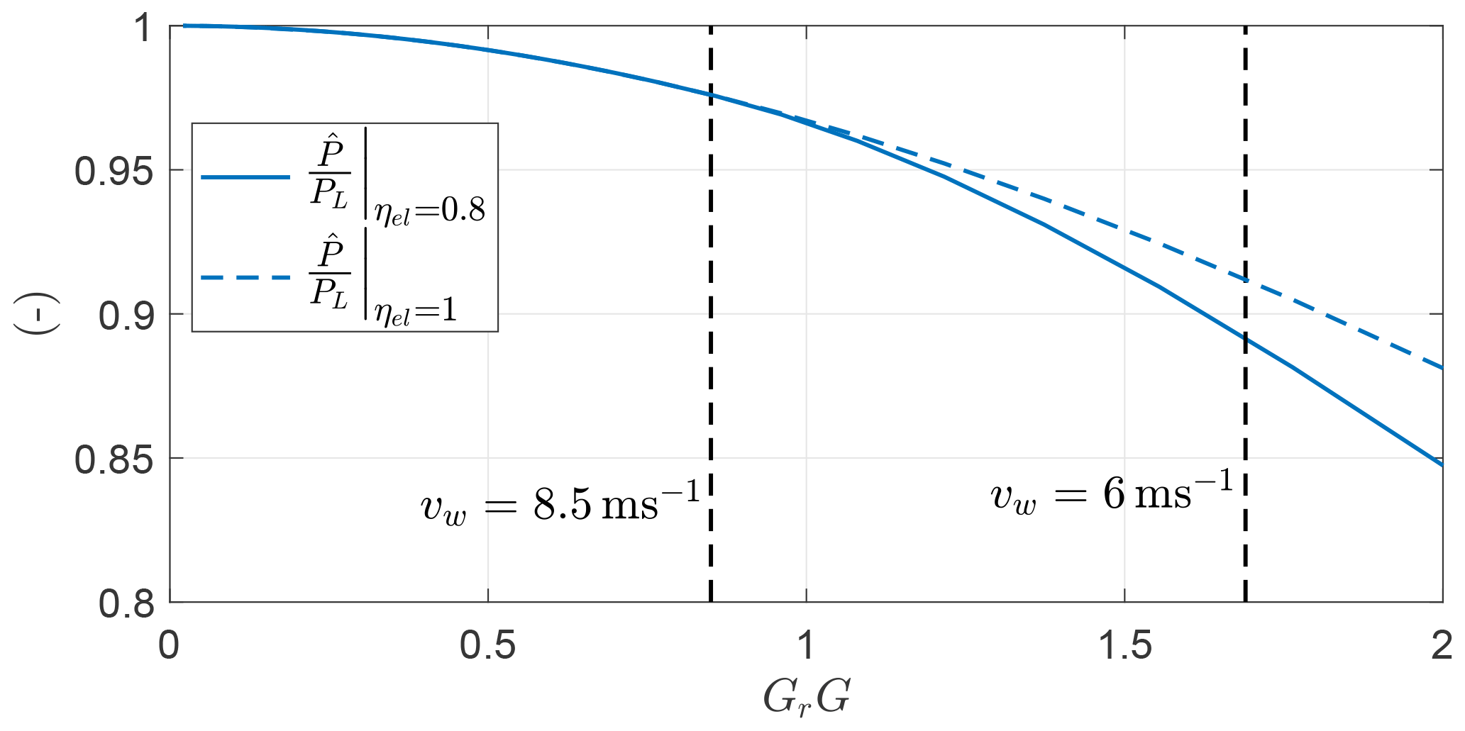
Figure 30 Normalized electrical power for a case with η_el=0.8 (−) and η_el=1 ($--$) as a function of G_rG.

To conclude, Fig. 31 shows the evolution of the first Fourier coefficient of the elevation angle A_β,1 and of the azimuth A_ϕ,1 as a function of G_rG. For high wind speed (i.e., low G_rG), their value is similar to the approximation given in Eq. (36). As G_rG increases, for η_el=1, A_ϕ,1 stays almost constant, while A_β,1 decreases. Smaller A_β,1 means smaller vertical height, which results in lower potential energy converted into electrical and kinetic energy over the loop. For η_el=0.8 after v_w=8.5 m s⁻¹, both Fourier coefficients decrease rapidly, meaning that smaller loops are performed. Smaller loops are therefore beneficial at low wind speed as they decrease the energy fluctuations.

Figure 31 Optimal values of A_β,1 and A_ϕ,1 normalized with the analytical expression of the opening angle $\stackrel{\mathrm{̃}}{\mathrm{\Phi }}$ for a case with η_el=0.8 (–) and η_el=1 (– –) as a function of G_rG.

6 Optimal control problem considering gravity, wind shear and elevation constraint

In this section, the wind shear is included in the problem. The reference altitude is h₀=100 m, the wind shear exponent is α_s=0.2 and the reference wind speed is $v_{\mathrm{w},\mathrm{0}}=\mathrm{6}$ m s⁻¹. To make the problem more realistic, a constraint on the minimum elevation angle of β_m=10^∘ (which is equivalent to a constraint on the minimum flight altitude) is included. The value of β_s needed to compute e₃ and then the spanwise unit vector s (Eq. 5) is taken as the mean elevation angle ${\mathit{\beta }}_{\mathrm{s}}=\widehat{\mathit{\beta }}$. With this definition, the case of no roll (ψ=0) is obtained when the wing span is in the plane perpendicular to the mean elevation angle, as in Trevisi et al. (2021).

Two OCPs are solved and they are summarized in Table 5. OCP A features five harmonics to model the control inputs, while OCP B has one harmonic to model the onboard wind turbine thrust and two for the roll, as in the previous sections. The two optimizations have similar mean electric power outputs, meaning that they are almost equivalent.

Table 5 Settings of the two optimal control problems maximizing the mean power considering gravity and wind shear.

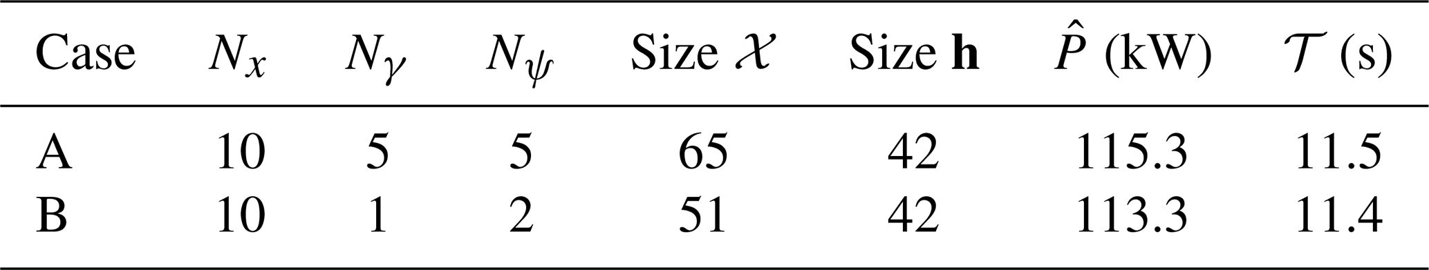
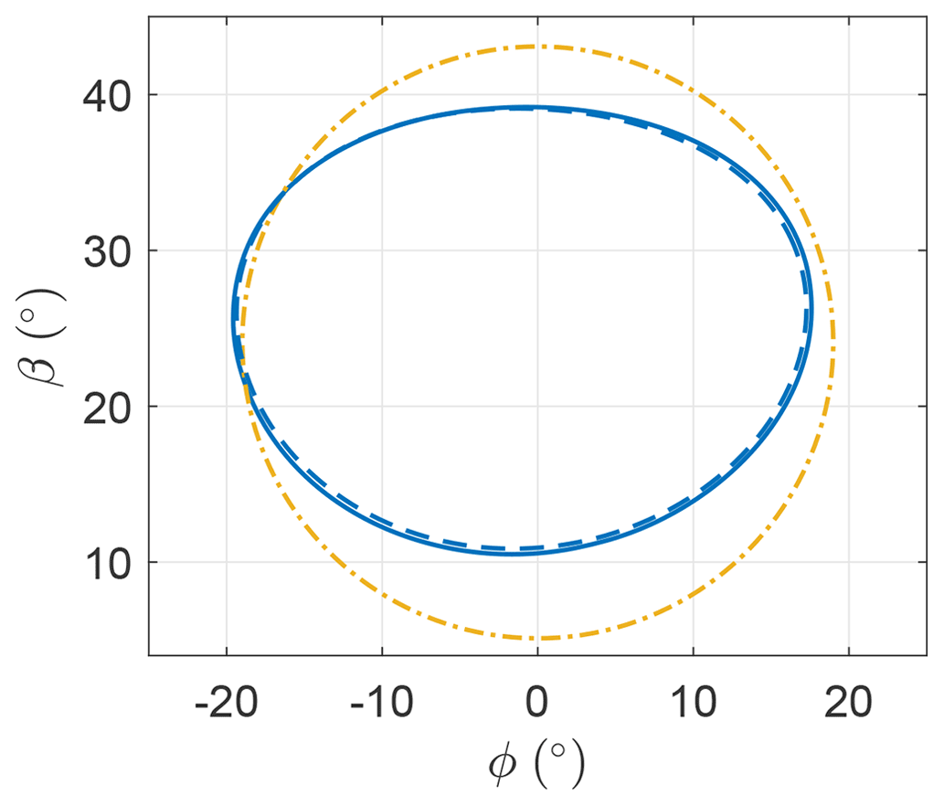
Figure 32 shows the trajectory for OCP A and B and compares it with a circle of radius $\stackrel{\mathrm{̃}}{\mathrm{\Phi }}$ centered at an elevation of $\widehat{\mathit{\beta }}=\arctan \sqrt{{\mathit{\alpha }}_{\mathrm{s}}}$, as this formulation identifies the elevation of the center of the wind power window (Argatov et al., 2011). As for the cases analyzed in Sect. 5.3 and 5.4, the trajectory is squashed along the vertical direction. The constraint on the minimum elevation angle is not used, as the trajectory of both cases is always strictly higher than β_m=10^∘.

Figure 32 Optimal trajectory for case A (−), case B ($--$) and a circle with radius Φ ($-.$).

The roll angle ψ is shown in Fig. 33. In LT-GliDe (Trevisi et al., 2021) the flight stability of AWESs is studied by linearizing the equations of motion with respect to a fictitious steady-state condition, where the AWES moves in a circular trajectory with a constant velocity. This steady state is characterized by the AWES span being perpendicular to the mean elevation angle direction. In this section, this condition is identified by ψ=0. The roll fluctuations, shown in Fig. 33, are limited in amplitude and might be considered within the linear bounds of the linearization validity of LT-GliDe. More analyses to prove this will be carried out in future works.

Figure 33 Optimal ψ as a function of the angular position.

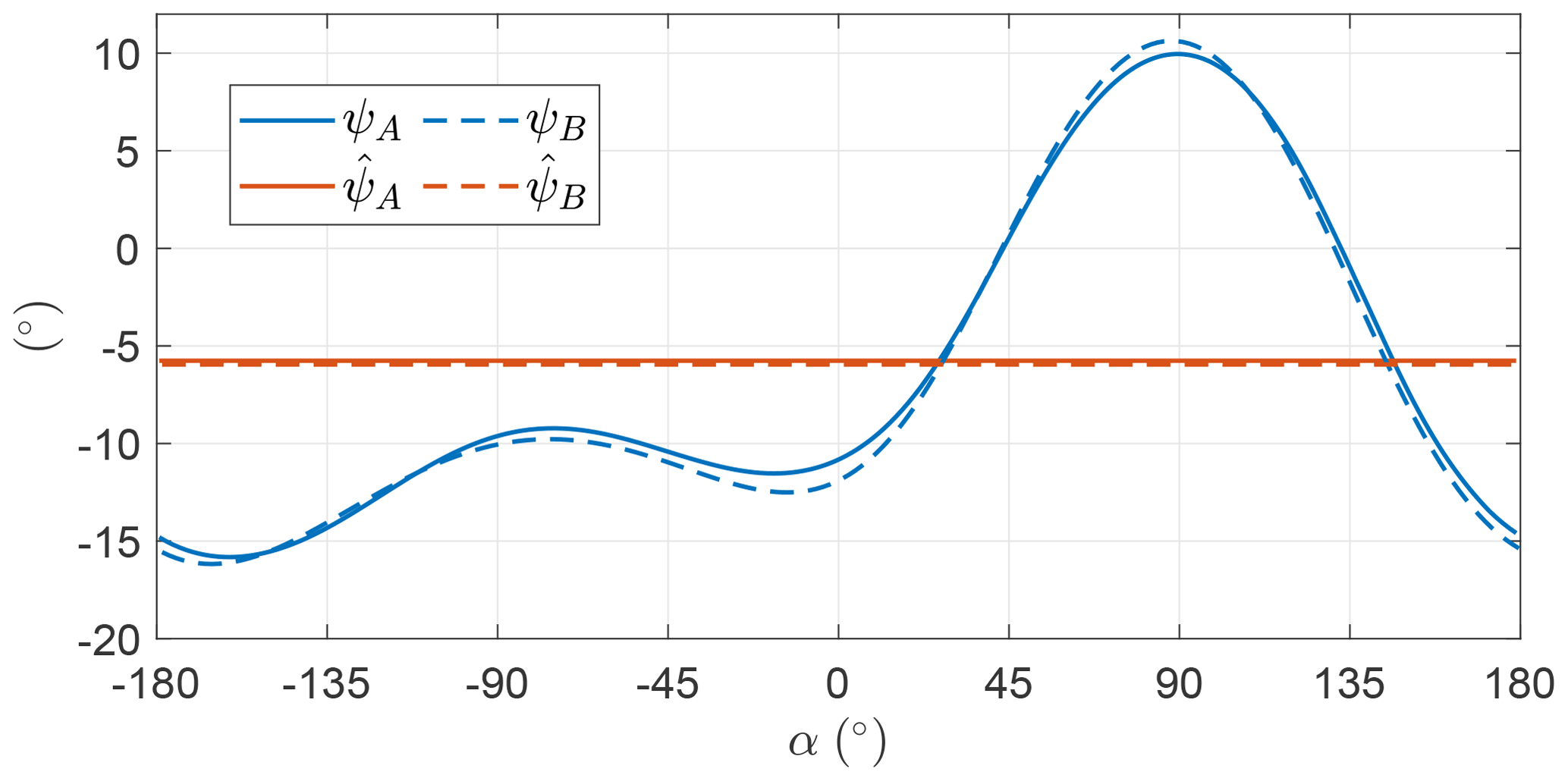
Figure 34 shows the evolution of the onboard wind turbine thrust coefficient as a function of the angular position for the two cases. The trends are similar to the analyses in Sect. 5.4. It is optimal to use the onboard wind turbines only to generate power and not as propellers. Even if the trends of γ for OCP A and B are quite different, the overall power production is similar, meaning that power production is not sensitive to harmonics of γ higher than one.

Figure 34 Optimal γ as a function of the angular position.

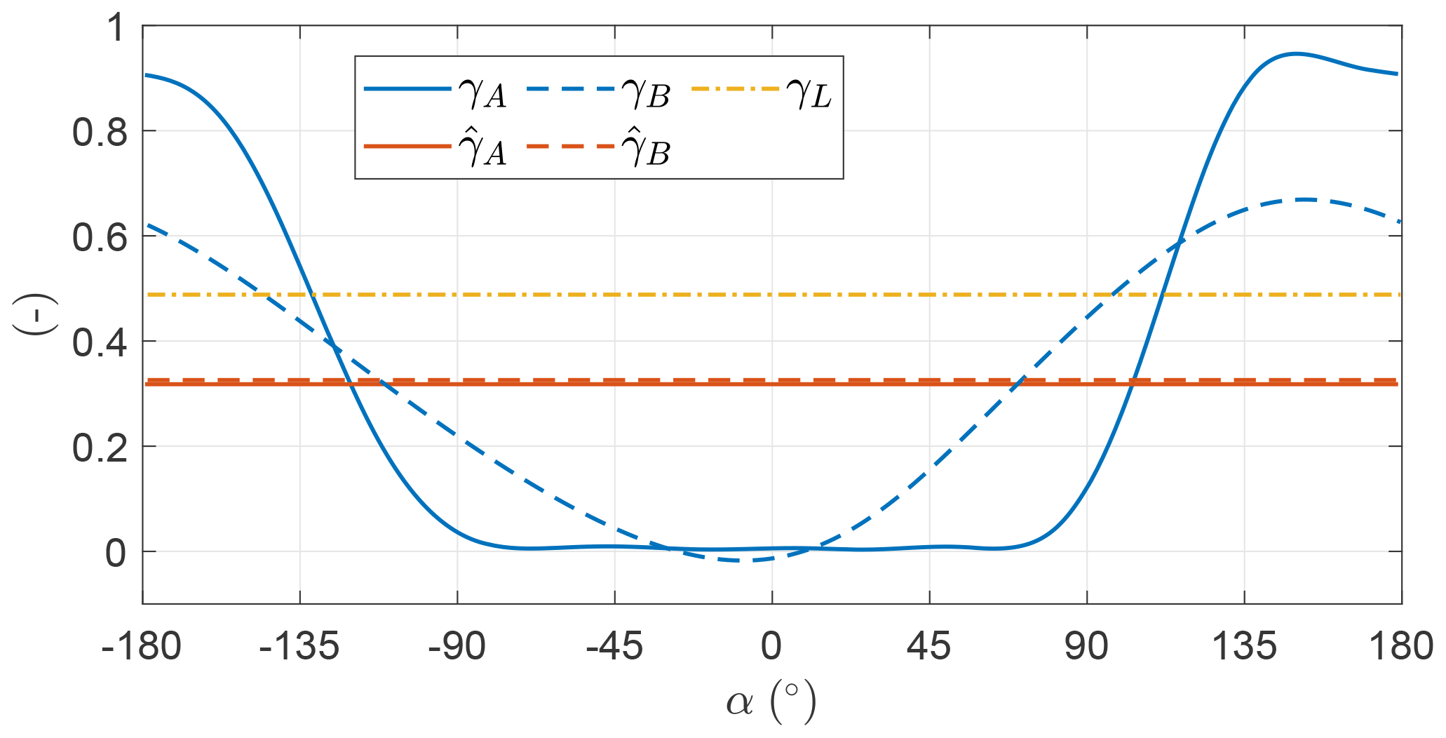
Figure 35 shows the wind speed that the AWES encounters over the loop due to the wind shear. Clearly, at the top of the loop (α=90^∘), the wind speed is the highest, sweeping approximately 1.5 m s⁻¹ over the trajectory. In this section, the mean wind speed over the loop is used to evaluate the Froude number Fr (Eq. 34) and consequently the gravity ratio G_r (Eq. 35). These numbers will be used later in this section to generalize results.

Figure 35 Wind velocity as a function of the angular position.

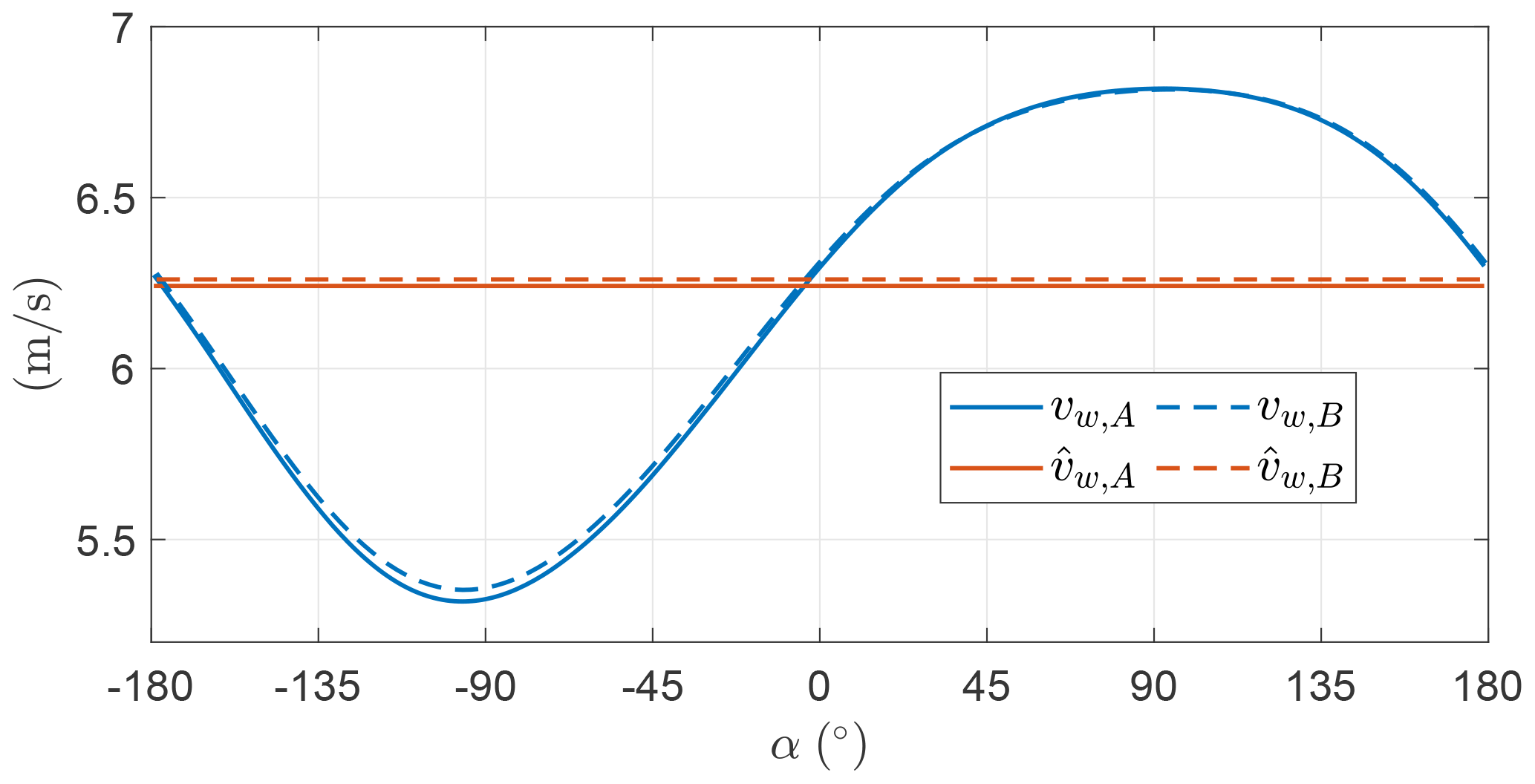
Figure 36 shows the AWES velocity as a function of the angular position. As discussed in the previous sections, in the descending leg the AWES converts the potential energy into electrical energy, producing power, and kinetic energy, accelerating. In the climbing leg instead, electrical power is not spent and kinetic energy is transformed into potential energy.

Figure 36 Norm of the optimal AWES velocity v as function of the angular position.

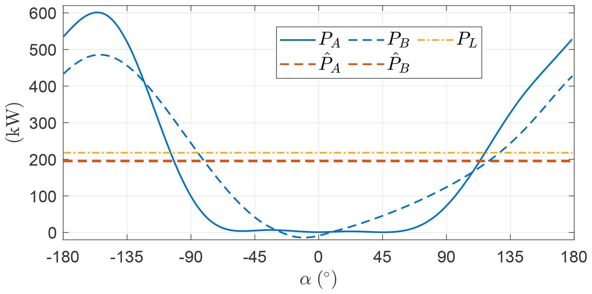
Figure 37 shows the power production as a function of the angular position. When looking at power and tether force (not shown here as it follows the AWES velocity trend squared) to characterize the operations of a real system, the maximum power and the maximum and minimum tether force would be constrained not to exceed some given values. To properly include these constraints, additional control inputs, useful to model the de-powering of the AWES (e.g., the lift coefficient), shall be considered in the analysis.

Figure 37 Optimal power production P as function of the angular position.

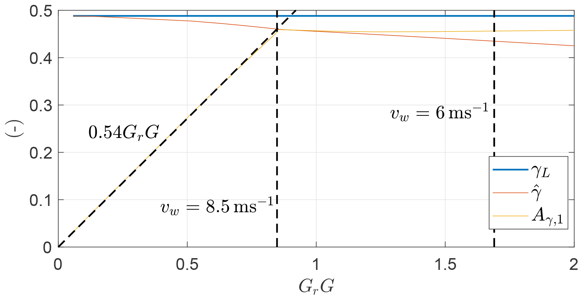
As carried out in the previous section, trends are studied as a function of the Froude number for the optimal control problem B. Figure 38 shows the dependence of $\widehat{\mathit{\gamma }}$ and A_γ,1 as a function of G_rG. $\widehat{\mathit{\gamma }}$ decreases when G_rG increases (i.e., the wind speed decreases). At low wind speed, $\widehat{\mathit{\gamma }}$ takes low values so that the AWES speed over the loop is higher, which is beneficial to stay airborne. A_γ,1 for low G_rG has a linear trend, as noted in Sect. 5.4. When A_γ,1 is equal to $\widehat{\mathit{\gamma }}$, the minimum power production over the loop is null. For lower wind speeds (i.e., higher G_rG), it is no longer optimal to increase A_γ,1 because the onboard wind turbines would be used as propellers with a high penalty on the mean power production.

Figure 38 Optimal values of $\widehat{\mathit{\gamma }}$ and A_γ,1 as a function of G_rG.

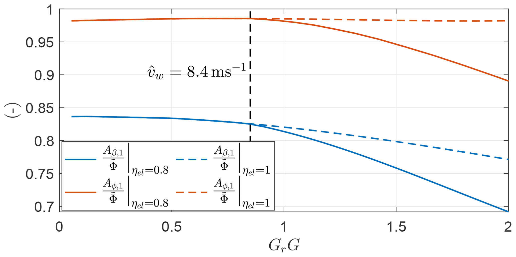
Figure 39 Optimal values of A_β,1 and A_ϕ,1 normalized with the analytical expression of the opening angle $\stackrel{\mathrm{̃}}{\mathrm{\Phi }}$ for a case with η_el=0.8 (−) and η_el=1 ($--$) as a function of G_rG.

To conclude, Fig. 39 shows the ratio of the first Fourier coefficient of β and ϕ with respect to the analytical expression of the opening angle $\stackrel{\mathrm{̃}}{\mathrm{\Phi }}$ for a case maximizing electrical power (η_el=0.8) and shaft power (η_el=1). After the cusp in Fig. 38, the two trends diverge, and for η_el=0.8 smaller loops are optimal so that the exchange of potential energy over the loop is reduced.

7 Conclusions and discussion

In this work, a novel methodology to study optimal trajectories for Fly-Gen AWESs is introduced. The chosen low-fidelity dynamic model is characterized by 2 degrees of freedom (the AWES is modeled as a point mass with constant tether length) and two control inputs. The degrees of freedom are the elevation and the azimuth angle. The control inputs are the roll angle, defined as the rotation around the relative velocity direction, and the onboard wind turbine thrust coefficient. An optimal control problem is formulated in the frequency domain through a harmonic balance method. Working with the Fourier coefficients of the time series, instead of the time series themselves, allows the potential reduction of the problem size, the implicit imposition of periodicity and the acquisition of an intuitive understanding of the results by analyzing the harmonic contributions. Moreover, the analytical gradient of the objective function and the constraints with respect to the optimization variables can be provided to the solver, allowing for a deep and fast convergence of the optimal solutions.

The MX2 design from Tucker (2020) is taken as a reference AWES to introduce the results. To isolate the effects of each physical phenomenon, results are presented with an increasing level of complexity from the most idealized case, and they are compared with analytical solutions from literature, whenever possible. A set of idealized case studies with no constraint on the minimum elevation angle and uniform wind inflow are initially studied. If gravity is neglected, the solution is steady, and it can be described by analytical expressions. If gravity is considered, three different optimal control problems, characterized by three different objective functions, are solved.

• i.

  If the mean thrust power (mechanical power neglecting onboard wind turbine induction) is the objective function, the optimal trajectories are circular, have a constant AWES velocity and the wing span is perpendicular to the incoming wind. To obtain this condition, all the potential energy is converted into electrical energy by the onboard wind turbines. At low wind speed, onboard wind turbines are then used as propellers in the ascendant part of the loop. The optimal power, the trajectory shape and the production strategy can be accurately approximated with analytical expressions.

• ii.

  If the mean shaft power (mechanical power considering onboard wind turbine induction) is the objective function, the potential energy, in the descending leg, is partially converted into electrical energy and partially into kinetic energy. This is because the power conversion penalizes solutions with high onboard wind turbine induction. Therefore, the velocity fluctuates over the loop, and the trajectories are squashed along the vertical direction to decrease the potential energy exchange.

• iii.

  If the mean power electrical provided to the grid is the objective function (i.e., the electrical efficiency is included), the onboard wind turbines never operate as propellers. If operated as propellers, power would be converted from mechanical into electrical while descending and from electrical into mechanical while ascending, leading to large power losses due to the electrical efficiency. This effect is found only at low wind speed, when propelling the AWES in the climbing leg maximizes the mean shaft power. Past a given wind speed, using the onboard wind turbines as propellers does not maximize the mean shaft power, and the influence of the electrical efficiency on the production strategy vanishes.

When the wind shear and a constraint on the minimum elevation angle are included in the optimal control problem for maximizing the electrical power, trends are similar to the case with uniform inflow. Therefore, the power production strategy does not heavily depend on the wind shear. For the analyzed example, the constraint on the minimum elevation angle is not active.

For all the analyzed cases, additional analytical approximations characterizing the solution are introduced. These approximations are found by modeling the control inputs with the lowest number of harmonics. The onboard wind turbine thrust can be modeled with just one harmonic and the roll with two harmonics without loss of generality of the results.

The results of this work align with the discussions in Tucker (2020) and have a strong mathematical foundation, as the trajectory and the control inputs are found by solving optimal control problems. These methods are planned to be applied, with appropriate modifications, to other AWE architectures and to other trajectory types. A comparison between circular and figure-of-eight trajectories is foreseen. Finally, the physical understanding and methods proposed here are envisaged to be incorporated into the design, analysis and optimization framework T-GliDe (Trevisi et al., 2022), with the aim of improving the power estimation and including an optimal control module.

Appendix A: Nomenclature

Latin symbols
Lt	Tether length
A	Wing area
At	Total onboard wind turbine area
Aγ,1	Amplitude of the first Fourier harmonic of γ
Aβ,1	Amplitude of the first Fourier harmonic of β
Aϕ,1	Amplitude of the first Fourier harmonic of ϕ
a	Onboard wind turbine induction
CL	Lift coefficient
CD	Drag coefficient
T	Norm of the tether force
vw	Norm of the wind velocity
v	Norm of the AWES velocity
v	AWES velocity
vr	Relative wind speed
M	Non-dimensional mass parameter
Mt	Modified non-dimensional mass parameter
m	AWES mass
G	System glide ratio

Gt	Modified system glide ratio
Gr	Gravity ratio
g	Inequality constraints
g	Gravitational acceleration
h	Equality constraints
R	Additional equality constraints in the frequency
	domain
Nx	Order of the Fourier series of the state variables
Nγ	Order of the Fourier series of the control input γ
Nψ	Order of the Fourier series of the control input ψ
Fg	Gravitational force
Pt	Thrust power
Ps	Shaft power
P	Electrical power
Fr	Froude number
Greek symbols
β	Elevation angle
ϕ	Azimuth angle
ψ	Roll angle
ρ	Air density
γ	Onboard wind turbine factor
𝒯	Revolution period
ω	Revolution frequency
α	Angular position in the loop
ηel	Electrical conversion efficiency
Φ	Opening angle of the trajectory
𝒳	Optimization variables
Symbols
⋅L	Quantity evaluated with the steady state (Loyd)
	model
$\widehat{\cdot }$	Mean value

Appendix B: Figures of comparison between frequency-domain formulation and time integration

Figure B1 Azimuth and elevation of the trajectory found with the harmonic balance method and the time integration scheme for a circular-shaped trajectory.

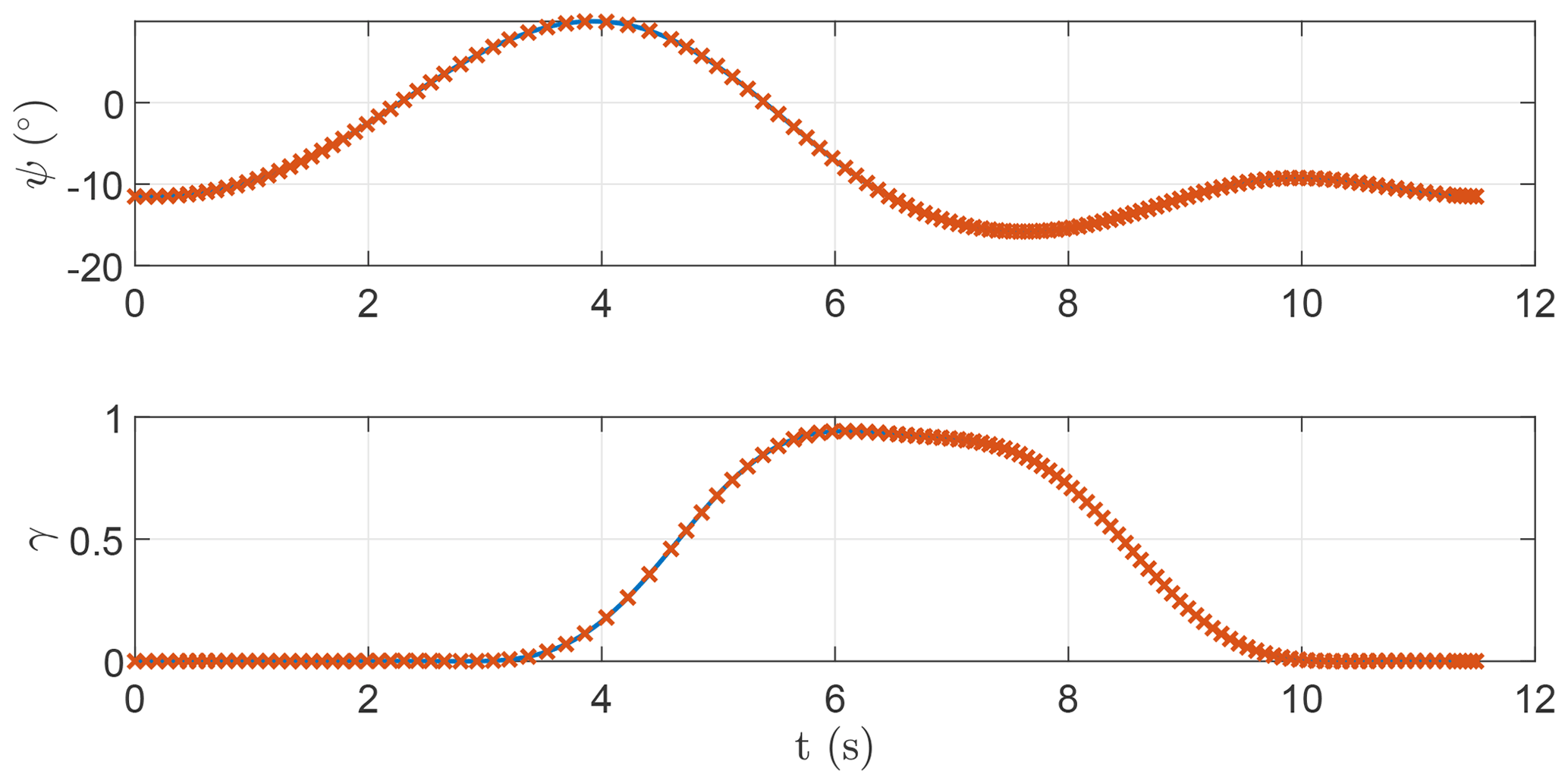
Figure B2 Time series of the control inputs provided to the harmonic balance method and the time integration scheme for a circular-shaped trajectory.

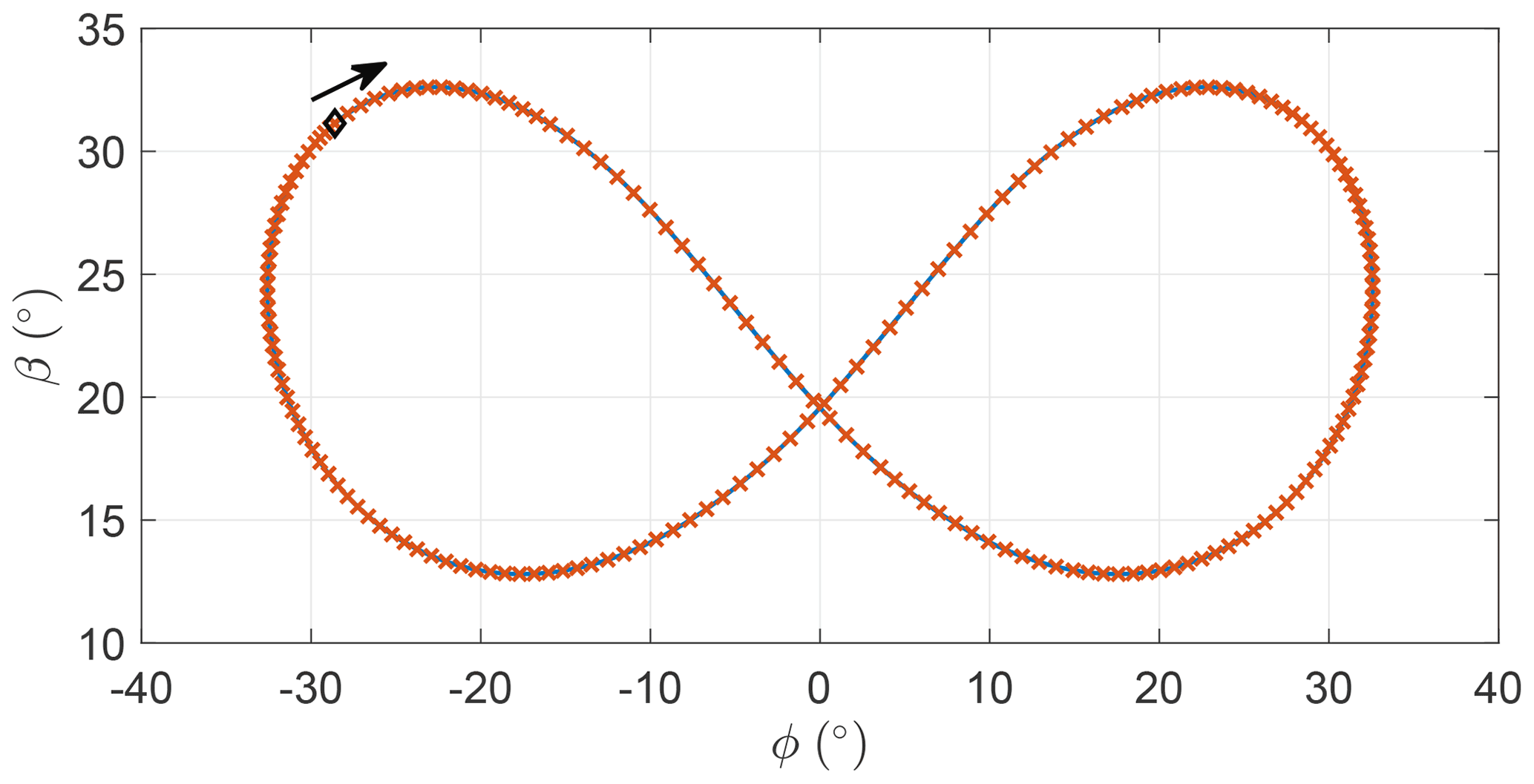
Figure B3 Azimuth and elevation of the trajectory found with the harmonic balance method and the time integration scheme for a figure-of-eight-shaped trajectory.

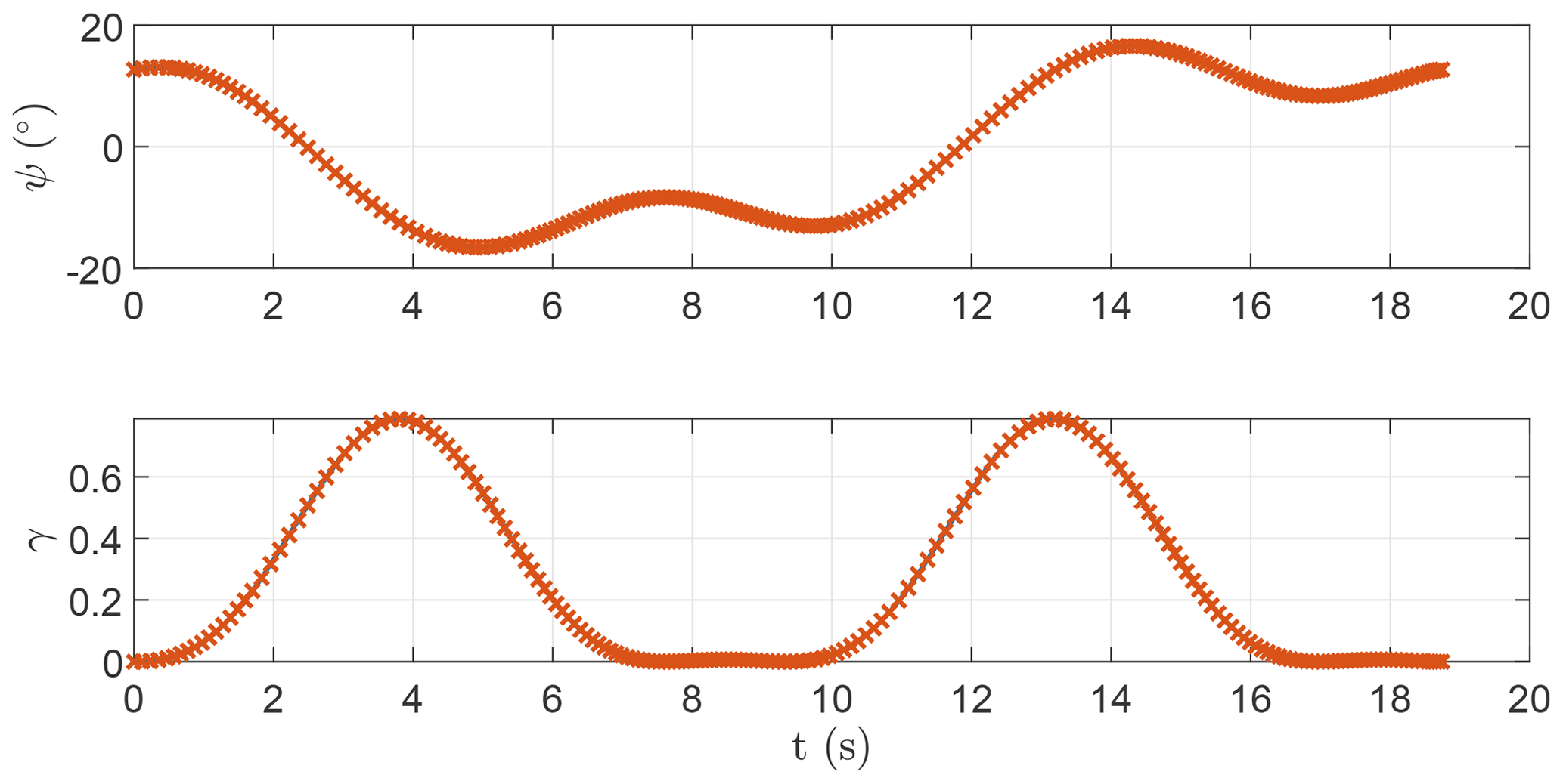
Figure B4 Time series of the control inputs provided to the harmonic balance method and the time integration scheme for a figure-of-eight-shaped trajectory.