Gaussian mixture model for extreme wind turbulence estimation

Uncertainty quantification is necessary in wind turbine design due to the random nature of the environmental inputs, through which the uncertainty of structural loads and response under specific situations can be quantified. Specifically, wind turbulence (described by the standard deviation of the longitudinal wind speed over a 10 min time duration) has a significant impact on the extreme and fatigue design envelope of the wind turbine. The wind parameters (mean and standard deviation of longitudinal wind speed over 10 min time duration) are not independent stochastic variables, and structural reliability analysis or uncertainty quantification therefore requires these wind parameters to be correlated stochastic parameters. An accurate probabilistic model should be established to model the correlation among wind parameters. Compared to univariate distributions, theoretical multivariate distributions are limited and not flexible enough to model the wind parameters from different sites or direction sectors. Copula-based models are often used for correlation description, but existing parametric copulas may not model the correlation among wind parameters well, due to limitations of the copula structures. The Gaussian mixture model is widely applied for density estimation and clustering in many domains, but limited studies have been conducted in wind energy and few have used it for density estimation of wind parameters. In this paper, the Gaussian mixture model is used to model the joint distribution of mean and standard deviation of longitudinal wind speed over 10 min time duration, which is calculated from 15 years of wind measurement time series data. As a comparison, the Nataf transformation (Gaussian copula) and Gumbel copula are compared with the Gaussian mixture model in terms of the estimated marginal distributions and conditional distributions. The Gaussian mixture model is then adopted to estimate the extreme wind turbulence (wind parameters for extreme load), which could be taken as an input to design loads used in the ultimate design limit state of turbine structures. The wind parameter contour associated with a 50-year return period computed from the Gaussian mixture model is compared with what is used in the design of wind turbines as given in IEC 61400-1. The Gaussian mixture model is able to model the joint distribution of wind parameters well, where the estimated tail distributions of both the marginal distributions and conditional distribution have good accuracy, and it is a good candidate for extreme turbulence estimation.

1 Introduction

Wind turbulence is characterized by the turbulence kinetic energy, its dissipation rate, and the length scale. This is modeled using three-dimensional anisotropic spectra that capture the auto-correlation and cross-correlation of the spatio-temporal wind speed variation, such as through the Mann model (Mann, 1994). Such models assume the wind turbulence is a Gaussian process, whereby several frequencies of wind velocity variations may occur, resulting in different wind velocities distributed as a function of time and space. Usually, the wind turbulence for wind turbine design is specified over a 10 min time window and the stochastic process is assumed to be stationary. The occurrence of extreme turbulence can then be categorized based on its return period. In wind turbine design, the wind turbulence with a 50-year return period is used in ultimate limit state analysis (IEC, 2019).

Many uncertainties exist in the evaluation of the design loads of wind turbine components. The IEC 61400-1 standard lists several load cases of the relevance of ultimate limit state analysis, wherein the load cases under normal operation usually require a partial safety factor (PSF) of 1.35 applied to the characteristic loads. Such PSFs are determined by quantifying the uncertainties in the load evaluation and the underlying distributions of the relevant inputs. An important load case towards determining ultimate design loads on wind turbine structures is the design load case (DLC) 1.3, in which the turbine is under normal operation under 50-year extreme wind turbulence. While relationships to evaluate the extreme turbulence level are provided in IEC 61400-1, there has been much debate on its accuracy and quantification, with edition-3 of IEC 61400-1 specifying a lognormal distribution for turbulence and edition-4 specifying it as a Weibull distribution. Several studies (Dimitrov et al., 2017; Abdallah et al., 2016) have proposed different models for extreme wind turbulence based on site measurements, and a large uncertainty can be seen in determining the long-term behavior of wind turbulence. Mathematically, an issue with the modeling of wind turbulence has been that the IEC 61400-1 standard and the literature are mainly focused on the probability distribution of the standard deviation of the wind speed (σ_u) conditional on the mean of the longitudinal wind speed over a 10 min time duration (u), whereas it is required that the joint distribution of σ_u and u is properly modeled.

A joint distribution model could be used for modeling multivariate random variables and generating random samples. Theoretical bivariate distributions are limited and not flexible enough. Monahan (2018) modeled the joint probability distribution of wind speeds at different locations using bivariate Rice distribution and bivariate Weibull distribution. The joint distribution of random variables could also be described by the univariate marginal distribution functions and a copula. A copula is a multivariate cumulative distribution function, where the marginal distribution follows a uniform distribution on the interval [0, 1]. Copulas are used for modeling the dependency among the random variables. Several families of copulas have been proposed in the literature, e.g., Gaussian copula (Nataf transformation (Xiao, 2014)) and Archimedean copulas (Bouyé et al., 2011). Using marginal distributions and copula to model the multivariate distributions is feasible, but the marginal distributions should be flexible enough to represent the wind inflow under varying environmental conditions, and the tail of the fitted distribution should be well representative of the actual inflow behavior. The copula structures should also be flexible enough to model different correlation structures. It is not clear which copula model (Abdallah, 2015) to choose to determine the joint distribution given marginal distributions.

To model extreme turbulence well, both the main body and the tail of the joint probability distribution of σ_u and u should be accurately represented. The Gaussian mixture model (GMM) is broadly used for clustering tasks (Zhang et al., 2021). GMM is a flexible model which can also perform density estimation on multivariate data with different marginal distributions and correlation structures. It is widely applied to different fields of study, e.g., speech and audio processing (Reynolds and Rose, 1995), image classification (Permuter et al., 2003), density estimation of microarray data in bioinformatics (Steinhoff et al., 2003), cancer classification (Prabakaran et al., 2019), and finance (Miyazaki et al., 2014). GMM is less commonly applied in wind energy compared to other domains, although Chang et al. (2017) used a GMM-based neural network for short-term wind power forecast, Cui et al. (2018) used GMM for fitting the probability distribution of wind power ramping features, Zhang et al. (2019) used GMM for wind turbine power dispatching, Li et al. (2020) used GMM for electrical loads forecast, and Srbinovski et al. (2021) used GMM for modeling the site-specific wind turbine power curves. GMM has been rarely adopted for wind parameter modeling, although Wahbah et al. (2018) used univariate GMM for wind speed probability density estimation, where the joint distribution of wind speed with other parameters was not investigated. Scarce published literature uses GMM for density estimation of wind inflow parameters and GMM has not been used for modeling the joint distribution of u and σ_u.

In this paper, GMM is used for modeling the joint distribution of the wind parameters u and σ_u. GMM is firstly used for density estimation of a random sample from a theoretical bivariate t distribution. It is then used for modeling the wind parameters from both offshore and onshore sectors. GMM is benchmarked to the measurement data by comparing the marginal distributions and the conditional distributions. The wind parameter contour with a 50-year return period is also computed from a GMM model with IFORM analysis (Winterstein et al., 1993). For the wind parameters from the offshore sector, Gaussian copula (Nataf transformation) and Gumbel copula are also compared.

2 Gaussian mixture model

GMM (McLachlan et al., 2019) is a mixture of several weighted Gaussian distributions and has been used for cluster analysis (Janouek et al., 2015) and density estimation (Steinhoff et al., 2003). GMM could be used for hard clustering and soft clustering of data. For hard clustering, each observation is assigned to the component returning the highest posterior probability, where each observation is assigned to exactly one cluster. Soft clustering, as opposed to hard clustering, assigns each observation to more than one cluster and each observation is assigned a responsibility (relative density). In terms of density estimation, the GMM is useful for multivariate distribution representations with multiple modes, but this does not prevent it from also being used for single-mode distributions. GMM is a linear combination of multivariate Gaussian distribution components, where each component is defined by its mean and covariance. Even though a weighted sum of Gaussian random variables is a Gaussian random variable, a weighted Gaussian distribution is not necessarily Gaussian. When there are more than two components for GMM, it is multi-modal and the distribution is not Gaussian. The probability distribution function (pdf) of a d-dimensional multivariate Gaussian is

$$\begin{array}{}\text{(1)}& \mathcal{N}\left(\mathit{x}|\mathit{\mu },\mathbf{\Sigma }\right)={\displaystyle \frac{\mathrm{1}}{\sqrt{\left|\mathrm{\Sigma }\right|(\mathrm{2}\mathit{\pi }{)}^d}}}\exp \left(-{\displaystyle \frac{\mathrm{1}}{\mathrm{2}}}(\mathit{x}-\mathit{\mu }){\mathrm{\Sigma }}^{-\mathrm{1}}{\left(\mathit{x}-\mathit{\mu }\right)}^{\mathrm{T}}\right),\end{array}$$

where μ is the 1-by-d mean vector and Σ is the d-by-d covariance matrix. The pdf of GMM is

$$\begin{array}{}\text{(2)}& p\left(\mathit{x}\right)=\sum _{j=\mathrm{1}}^k{\mathit{\pi }}_j\mathcal{N}\left(\mathit{x}|{\mathit{\mu }}_j,{\mathbf{\Sigma }}_j\right),\end{array}$$

where k is the number of components, which is a hyper-parameter, and π_j is the component coefficient (weight) and follows

$$\begin{array}{}\text{(3)}& \sum _{j=\mathrm{1}}^k{\mathit{\pi }}_j=\mathrm{1}\mathrm{0}\le {\mathit{\pi }}_j\le \mathrm{1}.\end{array}$$

Some information criteria are proposed in the literature (Akaike, 1998; Schwarz, 1978) to determine k, where k is selected as a balance of overfitting and underfitting. Nevertheless, when the sample size is too large, the criteria are not effective and further research is required. To use GMM for density estimation and also for random sample generation, the model parameters $\mathit{\{}{\mathit{\pi }}_j,{\mathit{\mu }}_j,{\mathbf{\Sigma }}_j$, j=1, 2, …, k} should be estimated from the data sample {x_n, n=1, 2, …, N}, where N is the sample size. The initial model parameters are calculated from the clusters evaluated by the k-means clustering algorithm (Arthur and Vassilvitskii, 2006), and optimized by the expectation-maximization (EM) algorithm (McLachlan et al., 2019) as follows:

1. Assign the N observations to the k clusters using the k-means clustering algorithm. Compute μ_j, Σ_j, and π_j from the observations within each cluster.

   The k-means clustering assigns N observations to k clusters, which are defined by the centroids. Each data point x_n with the closest centroid is assigned to the corresponding cluster. The centroids are recalculated and the data points are reassigned until the clusters do not change or the maximum iteration number is met. This is a hard clustering, and within each component, the μ_j and Σ_j are calculated, and the π_j is calculated as the number of data points in the current cluster divided by N.

2. Expectation-maximization (EM) algorithm: the model parameters $\mathit{\{}{\mathit{\pi }}_j,{\mathit{\mu }}_j,{\mathbf{\Sigma }}_j,j=\mathrm{1}$, 2, …, k} are found by an iterative EM algorithm (Dempster et al., 1977) to have a maximum likelihood estimation.

   • a.

     E step: evaluate the responsibilities using the current model parameters. The responsibility γ_j(x_n) is the probability that component j takes for explaining the observation x_n, which is calculated as

     $$\begin{array}{}\text{(4)}& {\mathit{\gamma }}_j\left({\mathit{x}}_n\right)={\displaystyle \frac{{\mathit{\pi }}_j\mathcal{N}\left({\mathit{x}}_n|{\mathit{\mu }}_j,{\mathrm{\Sigma }}_j\right)}{\sum _{i=\mathrm{1}}^k{\mathit{\pi }}_i\mathcal{N}\left({\mathit{x}}_n|{\mathit{\mu }}_i,{\mathrm{\Sigma }}_i\right)}}.\end{array}$$
   • b.

     M step: update the model parameters using the responsibilities from E step. The mean for component j is calculated as

     $$\begin{array}{}\text{(5)}& {\mathit{\mu }}_j={\displaystyle \frac{\sum _{n=\mathrm{1}}^N{\mathit{\gamma }}_j\left({\mathit{x}}_n\right){\mathit{x}}_n}{\sum _{n=\mathrm{1}}^N{\mathit{\gamma }}_j\left({\mathit{x}}_n\right)}}.\end{array}$$

     The covariance for component j is calculated as

     $$\begin{array}{}\text{(6)}& {\mathrm{\Sigma }}_j={\displaystyle \frac{\sum _{n=\mathrm{1}}^N{\mathit{\gamma }}_j\left({\mathit{x}}_n\right)\left({\mathit{x}}_n-{\mathit{\mu }}_j\right){\left({\mathit{x}}_n-{\mathit{\mu }}_j\right)}^{\mathrm{T}}}{\sum _{n=\mathrm{1}}^N{\mathit{\gamma }}_j\left({\mathit{x}}_n\right)}}\end{array}$$

     and the j component coefficient is calculated as

     $$\begin{array}{}\text{(7)}& {\mathit{\pi }}_j={\displaystyle \frac{\mathrm{1}}{N}}\sum _{n=\mathrm{1}}^N{\mathit{\gamma }}_j\left({\mathit{x}}_n\right).\end{array}$$

3. Repeat step 2 until the model parameters converge or the maximum number of iterations is met.

3 Results

GMM is proposed to model the joint distribution of u and σ_u, where the estimation error is small at both the main body pdf and the tail distribution. To verify the use of GMM, it is firstly used to recover the multivariate t distribution from a t distribution random sample. The flexibility of GMM (especially for modeling non-Gaussian joint distribution) and the demonstration of the procedure of using GMM for density estimation is detailed. To sample from the fitted joint distribution is very important, as many reliability analysis and uncertainty quantification applications require random samples as inputs. The random samples from GMM are compared with the random sample from the t distribution and wind parameters. To compute the number of components k, the value is increased from 1 until the estimated density function converges.

Table 1 Initial GMM parameters.

Table 2 Final GMM parameters.

Using copulas to develop non-Gaussian joint distributions of u and σ_u is initially attempted. A joint probability distribution of u and σ_u is then modeled by GMM. For estimating the extreme turbulence (wind parameter contour with 50-year return period), the accuracy of the tail distribution is important. The probability of exceedance of σ_u conditional on u from GMM is thus compared with the measurement data. To further examine the flexibility of GMM, the wind measurement data from both the offshore and onshore sectors are investigated and the 50-year wind parameter contours are compared.

3.1 Multivariate t distribution

The pdf of the d-dimensional multivariate Student's t distribution is

$$\begin{array}{}\text{(8)}& f(\mathit{x},\mathbf{\Sigma },v)={\displaystyle \frac{\mathrm{1}}{|\mathbf{\Sigma }{|}^{\mathrm{1}/\mathrm{2}}}}{\displaystyle \frac{\mathrm{1}}{\sqrt{(v\mathit{\pi }{)}^d}}}{\displaystyle \frac{\mathrm{\Gamma }\left(\right(v+d)/\mathrm{2})}{\mathrm{\Gamma }(v/\mathrm{2})}}\left(\mathrm{1}+{\displaystyle \frac{{\mathit{x}}^{\prime }{\mathbf{\Sigma }}^{-\mathrm{1}}\mathit{x}}{v}}\right),\end{array}$$

where Σ is a correlation matrix with a correlation coefficient 0.6 and v=5 is the degrees of freedom. The multivariate Student's t distribution generalizes the univariate Student's t distribution, and its marginal distributions all have univariate Student's t distribution. The marginal distributions of multivariate Student's t distribution have fatter tails than the normal distribution. A random sample with size 10⁵ is generated from the bivariate t distribution, and GMM is used to fit the bivariate t distribution.

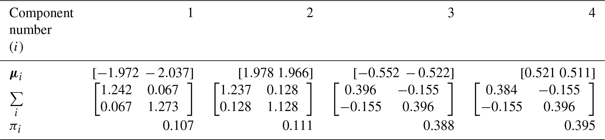
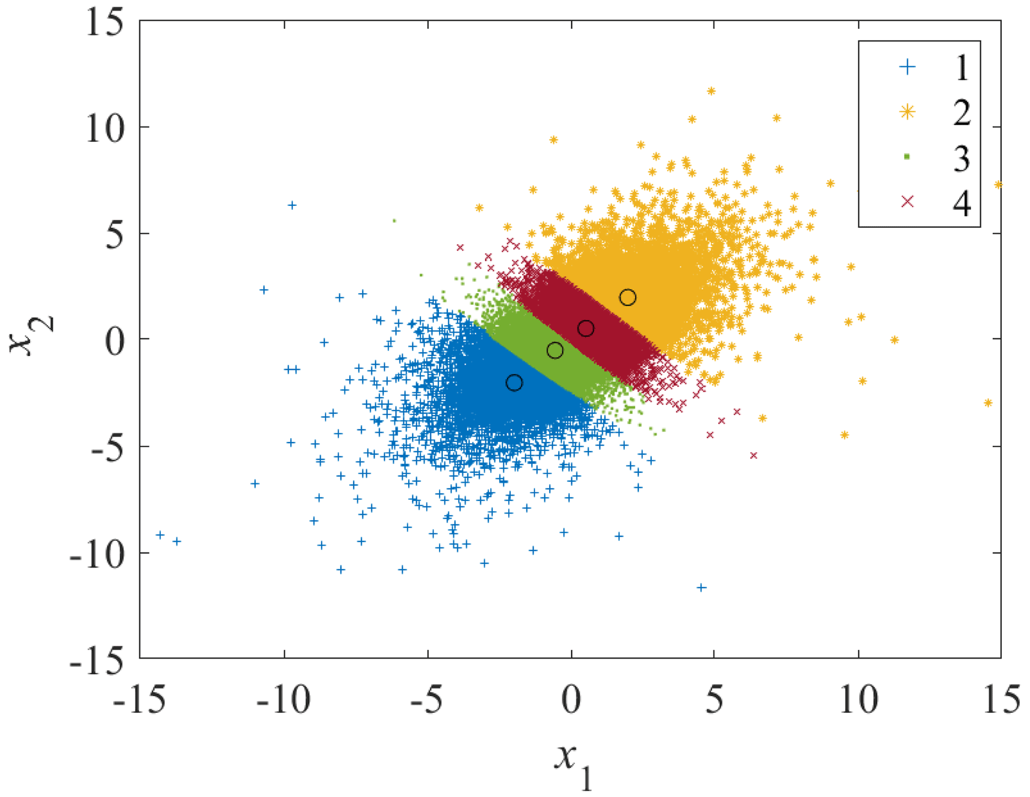
The estimated density function converges when the number of components k=4 and, therefore, the k-means clustering algorithm is used to cluster the data points into k=4 components. The mean, covariance, and the component coefficient (sample size at each component divided by the total sample size) calculated from each component are taken as initial parameters for GMM, which are shown in Table 1. The four clusters are plotted in Fig. 1, where the means are plotted in circles.

Figure 1 The k-means clustering of the t distribution sample.

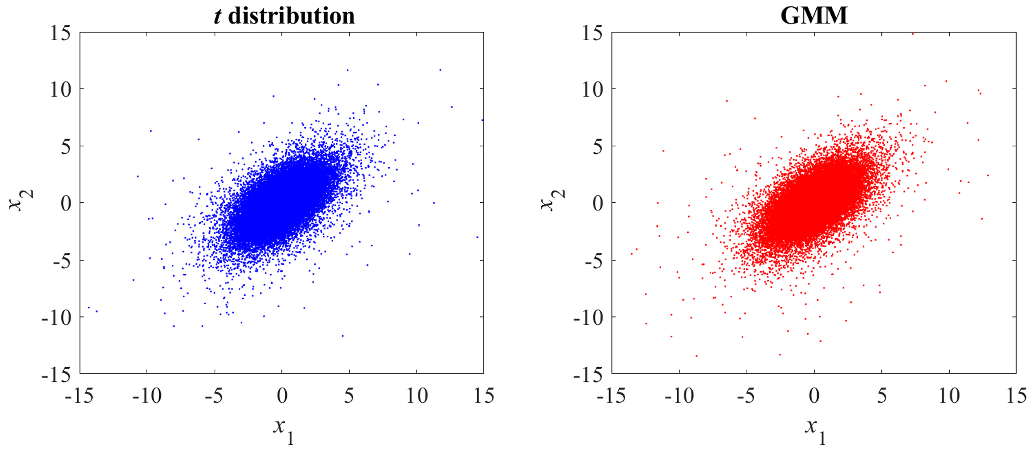
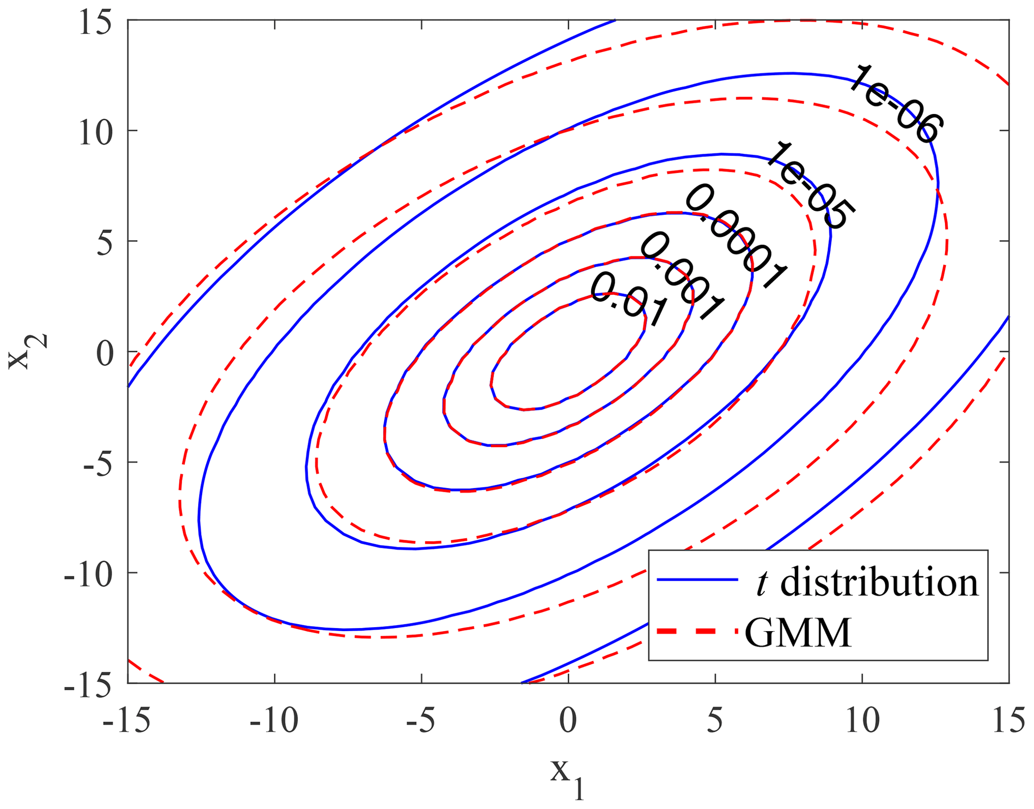
Following the procedure of the EM algorithm (see Sect. 2), the model parameters are estimated, which are shown in Table 2. Figure 2 shows the random sample from the t distribution and GMM, and Fig. 3 shows the corresponding contour plots. The random sample from GMM has a similar correlation structure to the theoretical t distribution. For probability densities higher than 10⁻⁵, GMM agrees well with the theoretical t distribution; for lower densities, there is some deviation, which is due to the small sample size and sample variation.

Figure 2 Random sample from the t distribution and GMM.

Figure 3 Contour plot of the t distribution and GMM.

3.2 Wind measurements

Wind measurements from the Høvsøre Test Centre for Large Wind Turbines in western Denmark (Dimitrov et al., 2017; Hannesdóttir et al., 2019) are used in this study. The 10 min high-frequency time series of three-dimensional wind velocities at a height of 100 m is selected. The period of measurements is from 1 January 2005 to 1 January 2020, i.e., 15 years of measurement data (Hannesdóttir et al., 2019). Values of u and σ_u, which are linearly detrended, are calculated from 10 min time series. The wind parameters from the offshore sector (225 to 315^∘) and onshore sectors (150 to 180^∘ and 45 to 135^∘) are studied here. Outliers and potentially missing data elements are omitted. The sensors on the Høvsøre mast are replaced regularly and calibrated, the data used in this paper are calibrated data (Peña Diaz et al., 2016). The sample size is about 2.43×10⁵ for the offshore sector, 4.09×10⁴ for the onshore sector (150 to 180^∘), and 1.41×10⁵ for the other onshore sector (45 to 135^∘). The wind speed variation is considered to be stationary, and non-stationary wind conditions are not included in this study.

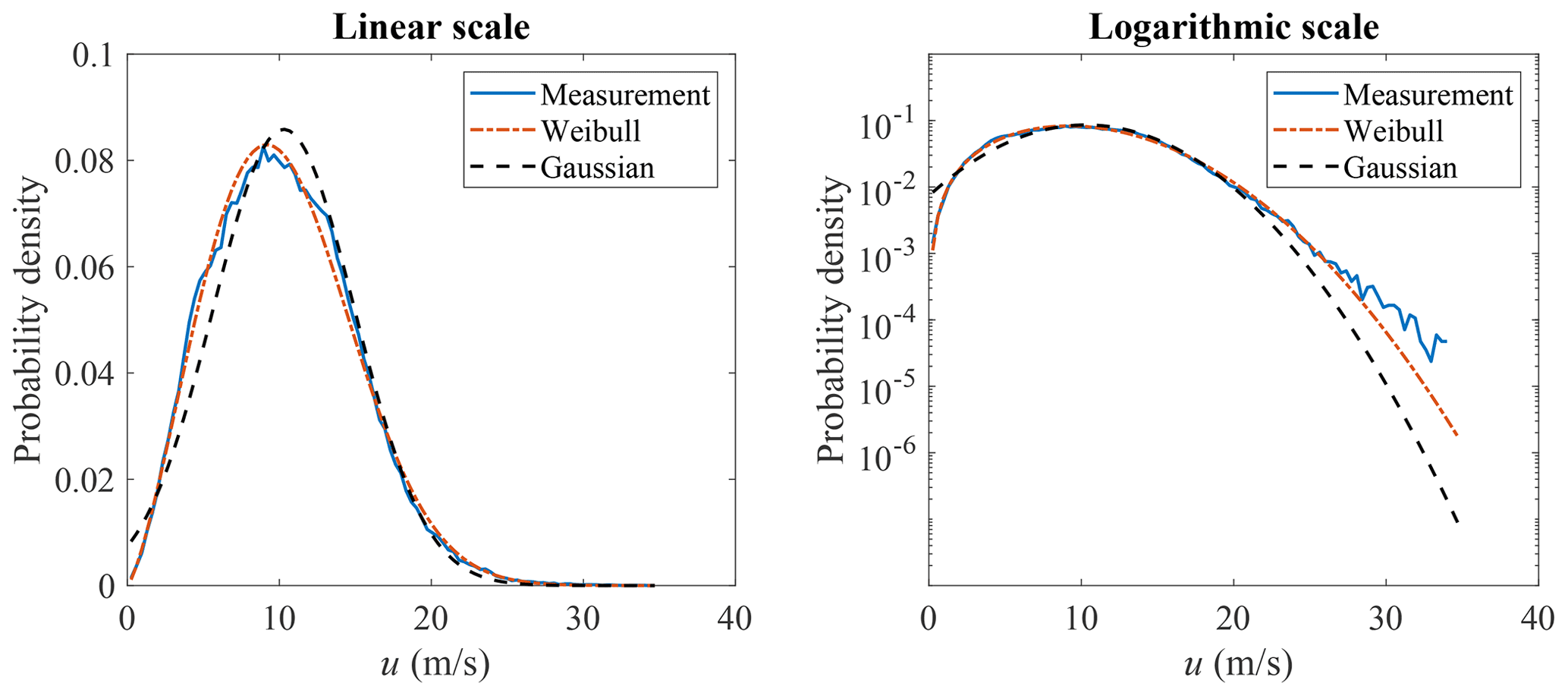
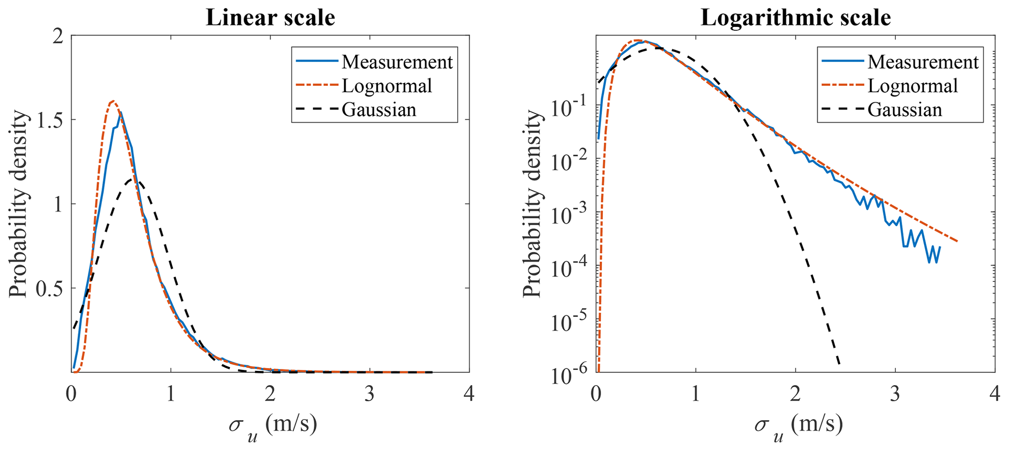
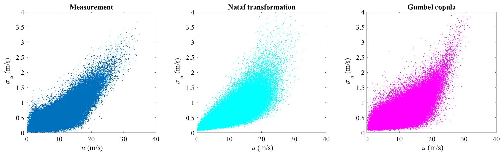
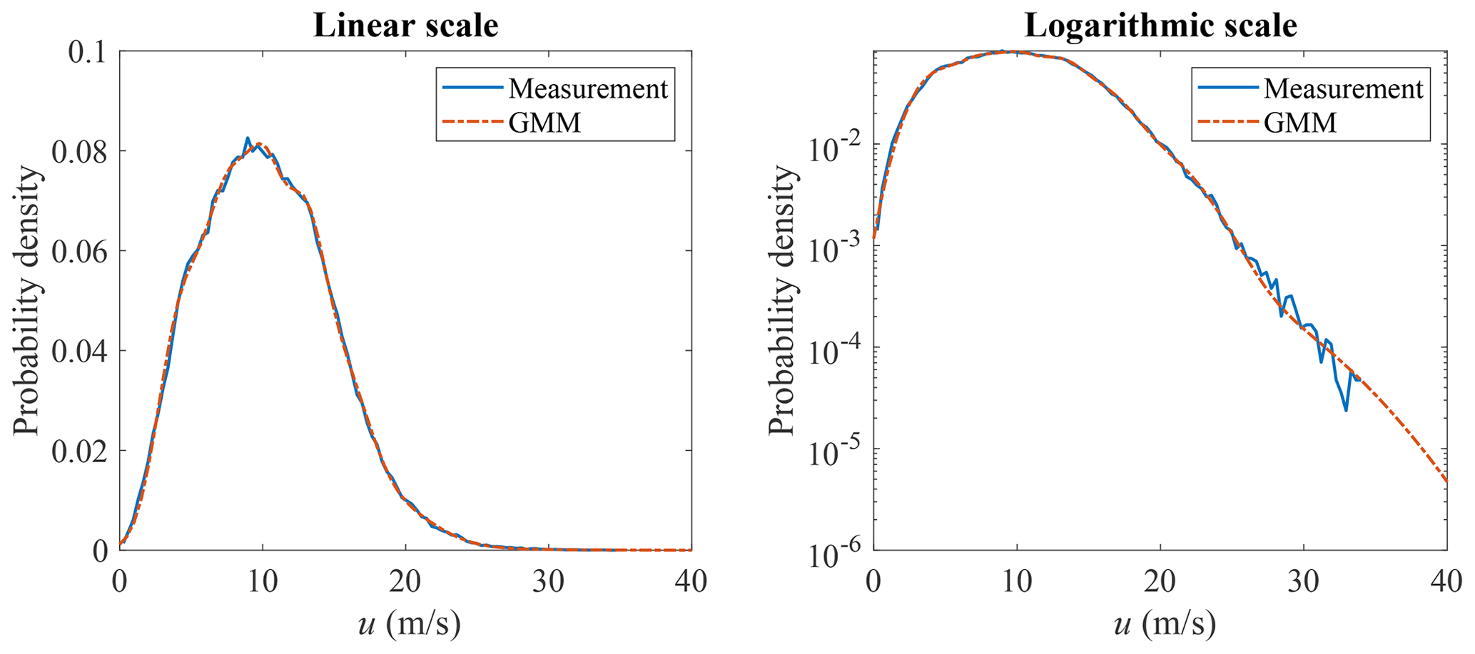
The marginal distributions to be used are to be defined and the correlation between the variables is modeled by the copula structure. Here, a Weibull distribution is used for modeling the marginal distribution of u, where the scale parameter is 11.61 and the shape parameter is 2.35. The plots are shown in Fig. 4. The lognormal distribution is used for modeling the marginal distribution of σ_u, where the mean and standard deviation of logarithmic values are −0.61 and 0.52. The plots are shown in Fig. 5. Both the linear and logarithmic scales are plotted, where the main body pdf and tail distribution could be compared. It can be seen that Weibull and lognormal distributions are good fits for u and σ_u, respectively. The univariate Gaussian distribution is also used here to fit the distribution of u and σ_u, but it is not a proper fit, which also indicates that the multivariate Gaussian distribution is not a good candidate for modeling the joint distribution of the wind parameters. The Nataf transformation (Xiao, 2014) and Gumbel copula are used here to model the joint distribution of u and σ_u and generate random samples. The generated random sample is shown in Fig. 6, where the left figure is the scatter plot of the measurement data, the middle figure is the Nataf transformation-generated sample, and the right figure is the Gumbel copula-generated sample. The Nataf transformation- and Gumbel copula-generated samples have the same sample size as the measurement data. They have the same fitted marginal distributions but different copula structures, as demonstrated in Fig. 6.

Figure 4 Marginal distribution of u with Weibull fitting.

Figure 5 Marginal distribution of σ_u with lognormal fitting.

Figure 6 Nataf transformation and Gumbel copula random samples for the offshore sector.

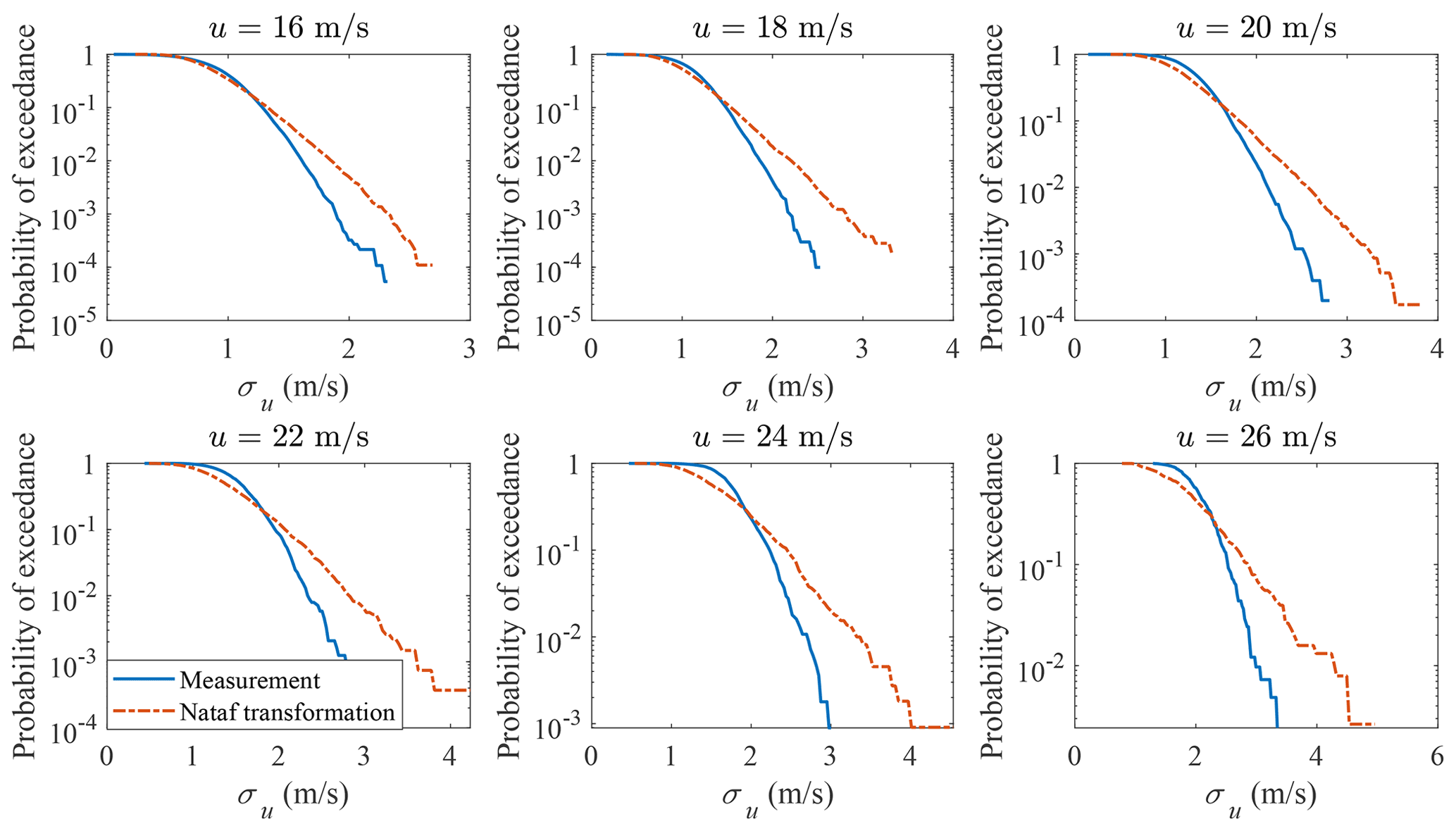
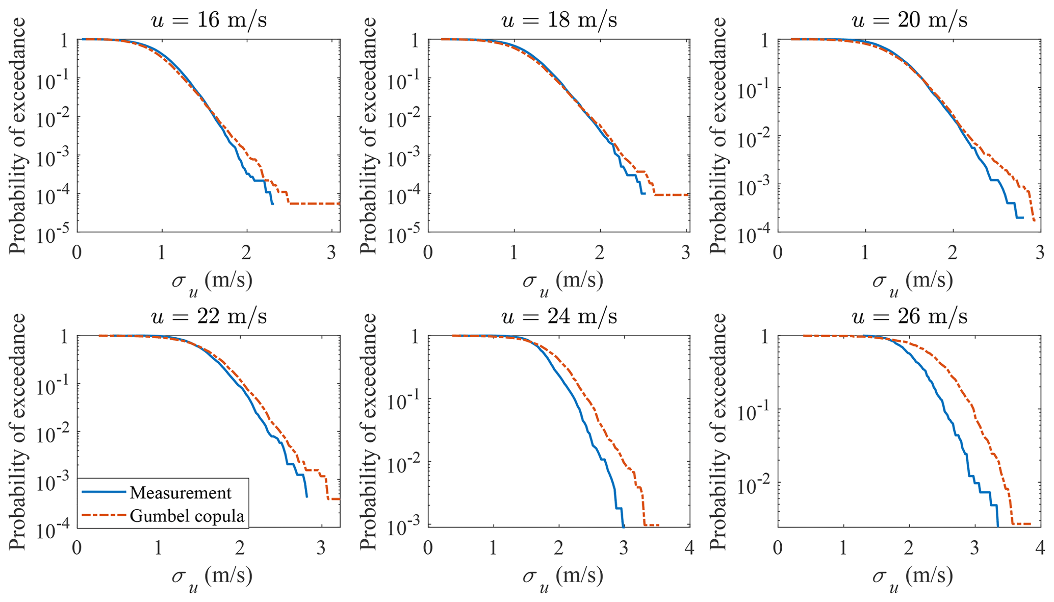
The different copula structures lead to different conditional distributions. The Nataf transformation- and Gumbel copula-estimated probabilities of exceedance of σ_u conditional on u are shown in Figs. 7 and 8, respectively. Only the distributions u≥16 m s⁻¹ are plotted, as they are close to the tail and affect the 50-year turbulence estimation most. As is seen in Fig. 7, the probabilities of exceedance of σ_u conditional on u deviate from the measurement data significantly. Using a Gumbel copula, as is shown in Fig. 8, even though there is a reasonable agreement when u ranges from 16 to 20 m s⁻¹, a larger discrepancy arises for higher mean wind speeds. The differences in the conditional distribution between the copula-estimated and measurement data indicate that using copula could lead to a biased 50-year turbulence estimation and large model uncertainty for DLC 1.3 simulations.

Figure 7 Nataf transformation probability of exceedance of σ_u conditional on u.

Figure 8 Gumbel copula probability of exceedance of σ_u conditional on u.

Even though other copula structures are available, they are not flexible enough to represent the joint distribution of u and σ_u from different measurement sites or even the same site for different wind direction sectors. The correct copula to use to generate the joint distribution of u and σ_u for tail estimation requires further research. However, instead of fitting the joint distribution using copula methods, a multivariate distribution is another option. To perform density estimation on univariate random variables, many theoretical probability distributions are available, e.g., normal, Weibull, lognormal, Rayleigh distribution, and the methods described in Zhang et al. (2020) and Low (2013), etc. On the other hand, fewer probability distributions are available for multivariate density estimations. This creates a similar limitation of copula models, i.e., theoretical multivariate distributions are limited and not flexible enough to model the u and σ_u measurements that possess different correlation structures. GMM on the other hand is quite flexible, since a number of Gaussian distributions with corresponding weights could be used to estimate the probability densities for multivariate variables and generate correlated samples.

Figure 9 Measurement data and GMM random sample for the offshore sector.

Figure 10 Marginal distribution of u for the offshore sector.

Figure 11 Marginal distribution of σ_u for the offshore sector.

3.3 GMM-based estimation of wind parameters for the offshore sector

It is important to model the joint distribution of wind parameters, which could be used for uncertainty quantification, structural optimization, and reliability analysis of wind turbines. The joint distribution should have a small estimation error for a realistic 50-year turbulence estimation. For the copula examples in Sect. 3.2, the marginal distributions are estimated well, but not the correlation structure, which leads to inaccuracies in the conditional distribution. Using GMM does not have the same limitation, as a good joint distribution estimation will estimate both marginal distributions and correlation structures with small estimation errors.

Figure 12 GMM probability distribution of σ_u conditional on u for the offshore sector.

Figure 13 GMM probability of exceedance of σ_u conditional on u for the offshore sector.

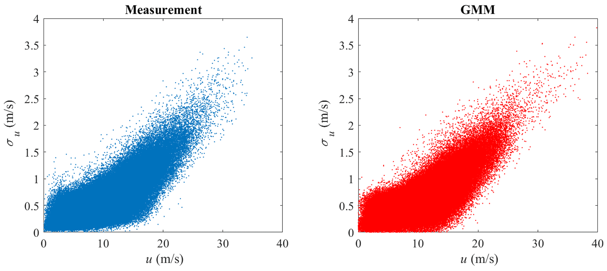
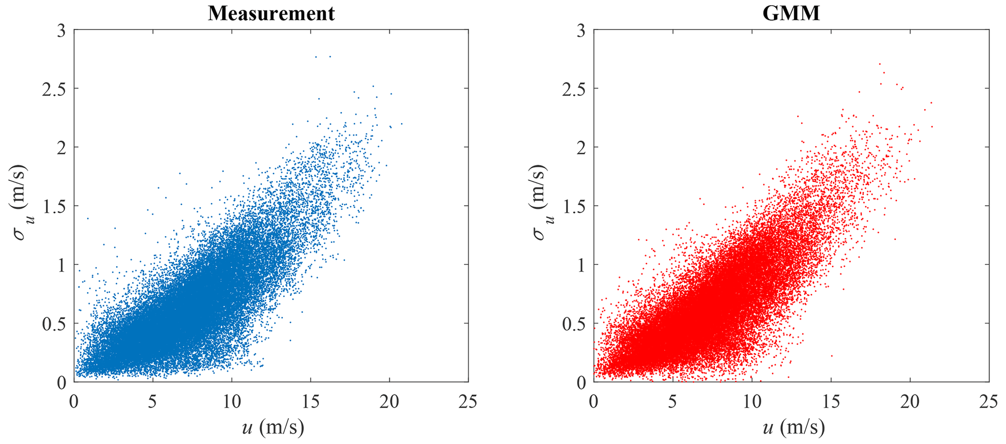
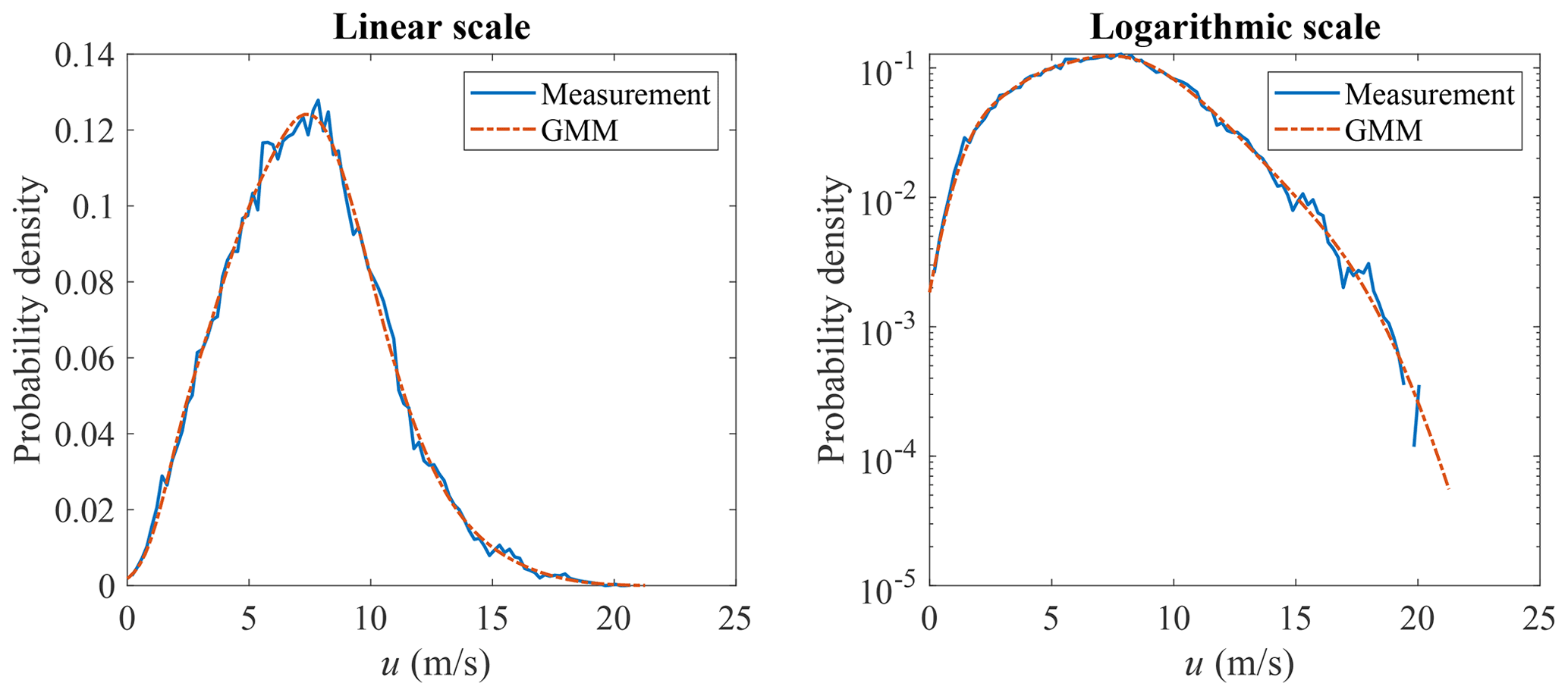
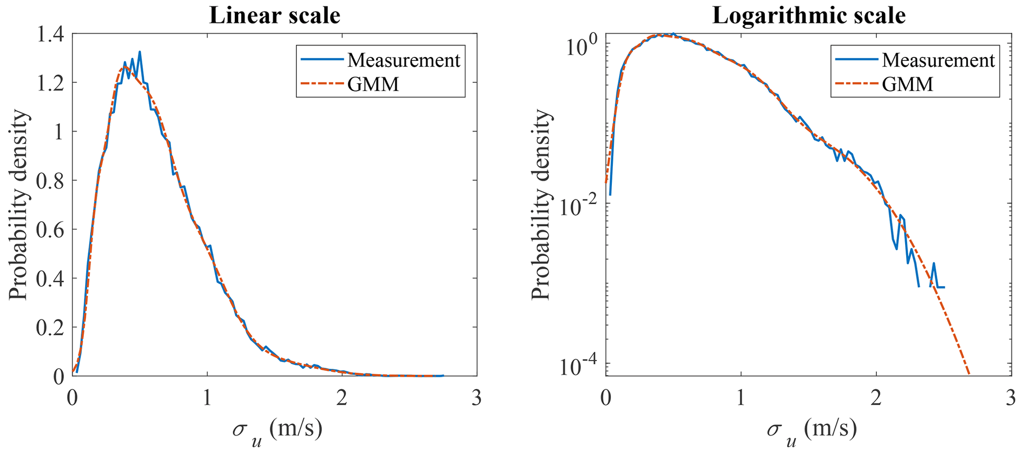
GMM is adopted here to model the joint distribution of u and σ_u. The measurement data and GMM random samples are shown in Fig. 9, where the correlation structure of the measurement data is well captured. The marginal distribution of u is shown in Fig. 10 and the marginal distribution of σ_u is shown in Fig. 11. Compared to Figs. 4 and 5, the marginal distributions from GMM have a smaller difference to the measurement data at both the main body pdf and the tails. The univariate Gaussian distribution is not a good fit for either of the marginal distributions, but GMM is a good fit, as its marginal distribution is a linear combination of univariate Gaussian distributions (not necessarily Gaussian distributions), which is more flexible compared to a Gaussian distribution. Which theoretical distribution to choose for marginal distribution estimation remains a problem, especially when the sample size is small and the tail might exhibit different shapes. GMM does not have the trouble of selecting distributions for marginal distribution estimation.

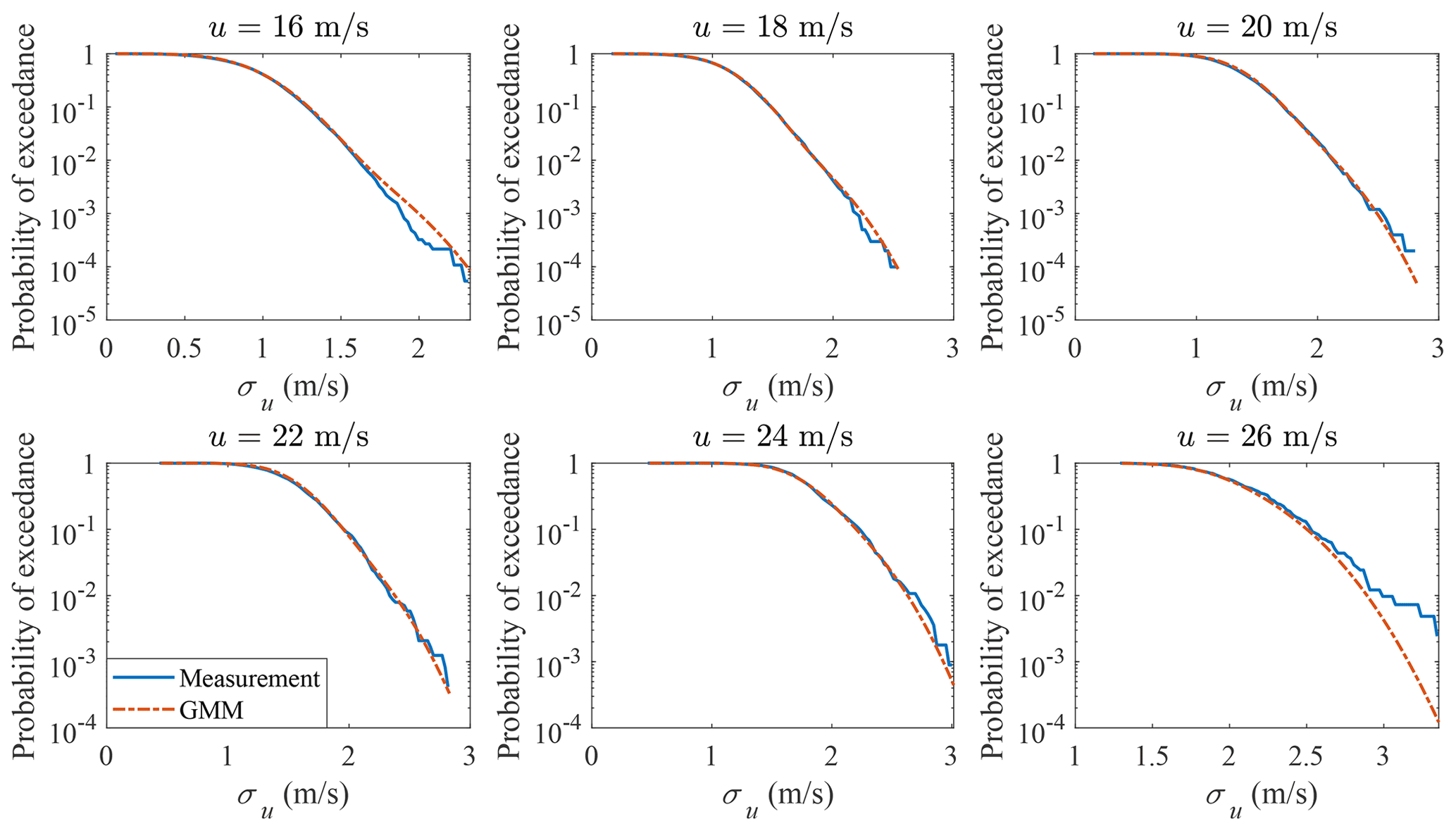
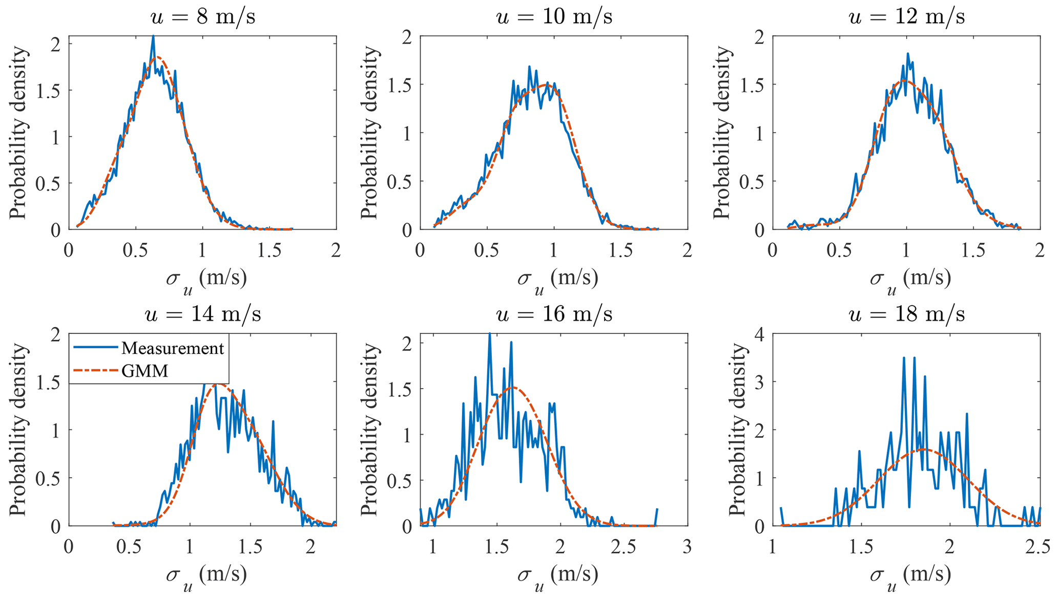
The probability distribution of σ_u conditional on u is plotted in Fig. 12. The probability of exceedance of σ_u conditional on u is plotted in Fig. 13. Both the main body pdf and the probability of exceedance from GMM agree quite well with the measurement data; for the bins when u=26 m s⁻¹, the tail of the measurement data is not accurate due to the small sample size (412).

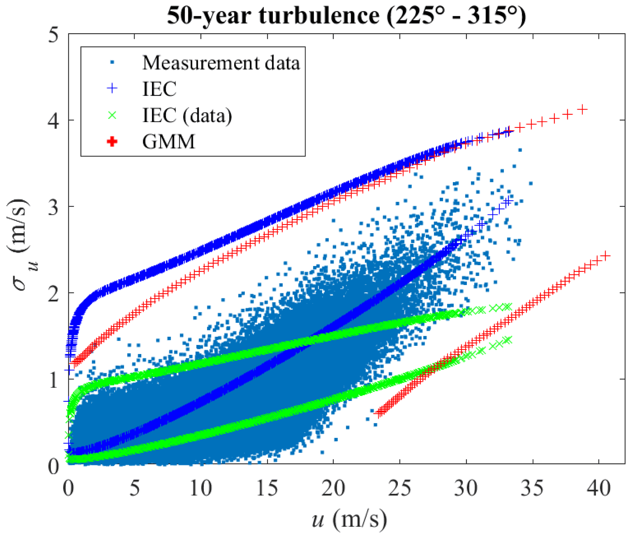
The 10 min turbulence level (wind parameter contours) associated with a return period of 50 years as provided in IEC 61400-1 and as computed by GMM are shown in Fig. 14. The contour labeled IEC (blue “+”) uses a reference turbulence intensity I_ref=0.12 (corresponding to wind turbine class C) as the input to perform IFORM analysis (Winterstein et al., 1993; IEC, 2005), where u is modeled by Weibull distribution and the probability distribution of σ_u conditional on u is modeled by lognormal distribution (IEC, 2005). The IEC (data) (green “x”) is the same as the IEC (blue “+”) except that I_ref=0.057, which is calculated as the expected value of turbulence intensity at a mean wind speed of 15 m s⁻¹ from the measurement data (IEC, 2005). The contour labeled IEC (data) has lower values than the contour labeled IEC, since I_ref is smaller (0.057 vs. 0.12). The 50-year contour estimated using GMM with IFORM analysis (Winterstein et al., 1993) is realistic, as it has a similar shape to the scatter plot of the measurement data and the most data points are inside the contour. The marginal distributions agree well with the measurement data (as are shown in Figs. 10 and 11), the conditional distributions are validated in Figs. 12 and 13. The IEC contour happens to be aligned with GMM, but IEC 61400-1 does not prescribe a joint probability distribution or the marginal distribution for σ_u. As the I_ref used is much larger than obtained through the measurement data (0.12 vs. 0.057), it could be inferred that the use of a lognormal distribution conditional on the mean wind speed or the empirical formulas in IEC (2005) might not be accurate. The fourth edition of the IEC 61400-1 (IEC, 2019) does not increase the accuracy with the Weibull distribution for turbulence conditional on the mean wind speed, as the 50-year turbulence level is still unchanged.

Figure 14 GMM and IEC 50-year turbulence estimation for the offshore sector.

3.4 GMM-based estimation of wind parameters for the onshore sectors

It is worth investigating the applicability of GMM to other wind direction sectors, where the wind parameters have different correlation structures due to different terrains. The u and σ_u in the onshore section (150 to 180^∘) are modeled using GMM. The measurement data and a random sample from GMM are shown in Fig. 15, where the correlation structure is different from the offshore sector in Fig. 9. The marginal distribution of u is shown in Fig. 16 and the marginal distribution of σ_u is shown in Fig. 17. Negligible differences could be seen in the comparison of the main body pdfs and the tails. The probability distribution of σ_u conditional on u is plotted in Fig. 18. The probability of exceedance of σ_u conditional on u is plotted in Fig. 19. Note that the sample size is smaller than for the offshore sector (4.09×10⁴ vs. 2.43×10⁵), so the tail distribution of the onshore measurement data has lower accuracy as compared to the offshore sector, but still performs better than using the method of copulas. The 50-year turbulence contour is shown in Fig. 20, where the left figure shows the 50-year turbulence estimated from the measurement data from the sector with direction from 150 to 180^∘, and the right figure is from the sector with direction from 45 to 135^∘. A slightly larger 50-year contour is estimated from the 45 to 135^∘ sector. Figures 18–20 show that GMM is indeed flexible and can be used to model u and σ_u for different wind conditions, albeit for flat terrains.

Figure 15 Measurement data and GMM random sample for the onshore sector.

Figure 16 GMM marginal distribution of u for the onshore sector.

Figure 17 GMM marginal distribution of σ_u for the onshore sector.

Figure 18 GMM probability distribution of σ_u conditional on u for the onshore sector.

Figure 19 GMM probability of exceedance of σ_u conditional on u for the onshore sector.

Figure 20 GMM and IEC 50-year turbulence estimation for two onshore sectors.

Note that the estimated density function converges when k=8 for all the joint distribution estimations of wind parameters using GMM. More components are needed compared to the theoretical t distribution (8 vs. 4), as the correlation structure between u and σ_u is more complex.

4 Conclusions

GMM is proposed to model the joint distribution of wind parameters, i.e., u and σ_u, and it is readily implementable and provides realistic 50-year turbulence levels. This model has been validated using multi-year high-frequency wind velocity measurements at one site for offshore climate and for flat land terrains. Copula-based joint probability models were not found to have the flexibility to accurately model the tails of σ_u conditional on u.

A procedure using GMM that properly captures the joint distribution of wind parameters is proposed. Both the marginal distributions of u and σ_u, and the distribution of σ_u conditional on u were shown to reflect the multi-year wind measurements. This model allows a good estimation of the 50-year turbulence (validated by the marginal and conditional distributions), which serves as an input to wind turbine design load cases. The procedure of GMM is demonstrated by fitting the theoretical multivariate t distribution. GMM is then used to estimate the probability distribution of offshore wind parameters and two-sector onshore wind parameters. There is good agreement between the GMM-estimated probability distribution and the measurement data. The 50-year wind parameter contour is estimated from GMM and compared with the corresponding values based on IEC 61400-1. The applicability to different sectors of the wind measurement data demonstrates its flexibility and shows its potential for modeling the joint distribution of wind parameters. Compared to copula methods, it has less estimation error for the estimated marginal distributions and conditional distributions.

Determination of the optimal number of components for GMM requires further research. In this paper, four components were found to be required to sufficiently model the theoretical t distribution and eight components were required to model the wind parameters for both offshore and onshore sectors of the chosen site. As more components are used, the pdf of GMM will converge to the target distribution, but will require more computational effort (several minutes on a standard laptop computer). Another limitation for GMM is that it might not extrapolate well for certain correlation structures, especially if the sample size is small, even though the model is quite flexible.