Four-dimensional wind field generation for the aeroelastic simulation of wind turbines with lidars

Lidar-assisted control (LAC) of wind turbines is a control concept that takes advantage of a nacelle-mounted lidar (a remote sensing device) to measure upstream wind speeds of a turbine to allow a preview of the incoming turbulence. Because the turbine will not be exposed to the identical turbulence as that measured by the lidar in advance, the simulation of a LAC system will be more realistic if wind evolution can be modeled in the wind field generation. Since the commonly used 3D stochastic wind field generation method does not include wind evolution, the main goal of this research is to extend the 3D method to 4D to enable the modeling of wind evolution along the wind direction. The most novel part of this research is that we propose a two-step Cholesky decomposition approach for the factorization of the coherence matrices in the wind field generation. With this approach, 4D wind fields can be generated by combining multiple statistically independent 3D wind fields. To enable better integration of the 4D method into the common workflow of wind turbine simulations, we implement the 4D method as the open-access tool evoTurb in combination with TurbSim and Mann turbulence generator. Moreover, since 4D wind field generation is supposed to be coupled with lidar simulations, and considering the range weighting effect of lidars and eventually multiple range gates, a 4D wind field will contain many more simulation points than a 3D one. To avoid excessive computational effort, we further investigate the impacts of the spatial discretization in 4D wind fields on lidar simulations to provide some insights to optimize the application of 4D wind field generation.

1 Introduction

Wind turbines are highly dynamic systems operating in turbulent wind fields in the atmospheric boundary layer, with interacting effects of aerodynamics, structural dynamics, control systems, soil dynamics, and hydrodynamics (only for offshore locations) (Moriarty and Butterfield, 2009). Simulation of wind turbine systems requires algorithms to properly generate inflow turbulence. Although computational fluid dynamics (CFD) such as direct numerical simulations or large eddy simulations (LESs), which solve the Navier–Stokes equations numerically, produce more realistic turbulence in the physical sense, these algorithms are computationally too expensive for engineering design. Therefore, in the wind energy industry, stochastic wind field simulations are mainly applied. There are two commonly used tools for that: TurbSim, provided by the National Renewable Energy Laboratory, and the Mann turbulence generator, made available by DTU Wind Energy, Technical University of Denmark.

TurbSim was initially developed on the basis of the 3D wind field simulation method proposed by Veers (1988), known as the Veers method (Jonkman, 2009). This simulates stationary multidimensional random processes with specified cross-spectrum densities to generate turbulent wind velocities. Several spectral models of turbulence are available in TurbSim, of which the most commonly used model is the Kaimal spectral and exponential coherence model (Kaimal et al., 1972) (hereinafter referred to as the Kaimal model) – one of the two turbulence models provided in ().

The Mann turbulence generator (MTG) is based on the Mann uniform (Mann, 1994) shear model (hereinafter referred to as the Mann model), which is another turbulence model given in (). In contrast to the Kaimal model which is formulated based on Kolmogorov's (Kolmogorov, 1941) $-\mathrm{5}/\mathrm{3}$ law, the Mann model combines the spectral tensor with the rapid distortion theory, which implies a linearization of the Navier–Stokes equation, and the modeling of the eddy lifetimes to include more physical considerations in the stochastic modeling of turbulent properties. Moreover, the computational method included in MTG is demonstrated in Mann (1998), which uses 3D inverse fast Fourier transformation (3D IFFT) (Heideman et al., 1985) to improve the computational efficiency.

It is worth mentioning that both tools create a 3D wind field: TurbSim creates time series of wind vectors at points in a 2D vertical rectangular grid fixed in space, namely $\mathbf{V}(t,y,z)$ (Jonkman, 2009); MTG creates a 3D wind field in space, namely $\mathbf{V}(x,y,z)$, and applies Taylor's (Taylor, 1938) frozen hypothesis to convert the x axis (aligned to the mean wind direction) to time axis by assuming that the turbulent wind field remains unchanged and propagates with the mean wind speed. Having such 3D wind fields is sufficient for the aeroelastic simulation of wind turbines with a feedback control system, and the application of Taylor's hypothesis is also justified because, in principle, only turbulence acting on the turbine needs to be considered in this case. However, that is not sufficient for modeling a lidar-assisted control (LAC) system, which takes advantage of a nacelle-mounted lidar, i.e., a remote sensing device that can measure wind speeds in front of the wind turbine using Doppler effect (Weitkamp, 2005), to allow the wind turbine to proactively adjust to the incoming turbulence (see, e.g., Bossanyi et al., 2014; Schlipf, 2015; Simley, 2015; Simley et al., 2018). The reason for that is that the LAC system uses turbulence signals taken at some distance upwind as input, but the turbulence will evolve before it reaches the turbine – this physical phenomenon is called wind evolution (Chen et al., 2021). Thus, the turbine will not be exposed to exactly the same disturbances as that measured by the lidar (Guo and Schlipf, 2021). To make it possible to simulate this effect in stochastic wind field simulations and to assess the benefits of LAC more reasonably, Taylor's hypothesis should no longer be applied, and wind evolution must be taken into account.

Wind evolution refers to time-dependent variation of turbulence structures (eddies). In practice, wind evolution is usually quantified with the longitudinal coherence between the wind speeds measured at different locations in the mean wind direction (see, e.g., Pielke and Panofsky, 1970; Kristensen, 1979; Simley and Pao, 2015; Schlipf et al., 2015; Chen et al., 2021). As reviewed in Chen et al. (2021), two types of wind evolution models have been proposed in previous research. On the one hand, an empirical model which is a simple exponential function with a single decay parameter was initially suggested by Pielke and Panofsky (1970), following the study of Davenport (1961). Subsequently, Panofsky and Mizuno (1975) studied the correlations between the decay parameter and other wind-field-related parameters and suggested the first parameterization model for the exponential wind evolution model. On the other hand, Kristensen (1979) believed that the longitudinal coherence should have different properties than the lateral and vertical coherence and deduced another model form based on modeling the probability of eddy decay and eddy transversal diffusion. In recent years, Simley and Pao (2015) modified the exponential wind evolution model by including a second parameter to adjust the coherence at very low frequency, taking a similar model form as the coherence model for transverse and vertical separations proposed by Thresher et al. (1981), and suggested a model to determine both model parameters based on LESs. On the basis of Simley and Pao's model (Simley and Pao, 2015), Chen et al. (2021) suggested a concept to build parameterization models using supervised machine learning (ML) algorithms and presented the results of Gaussian process regression models. In a following work, the performance of different ML algorithms was compared considering their computational efficiencies (Chen and Cheng, 2020).

Some attempts have been made to simulate the effect of wind evolution or integrate wind evolution models into 3D simulations. For example, Laks et al. (2013) proposed an approach to extend the Veers method (Veers, 1988) from the original wind field simulated on the rotor plane to an additional vertical plane in the inflow direction for generating preview measurements of lidars. Bossanyi (2013) suggested a method to simulate an evolving turbulent wind field with two random realizations of wind fields, which is implemented in Bladed – a simulation tool for wind turbine performance and load calculations (DNV-GL, 2016). However, both methods are intended to generate unfrozen turbulence on two different vertical planes, which are not directly applicable to the current commercial lidars that are able to measure at multiple upstream distances. de Maré and Mann (2016) extended the 3D Mann spectral tensor (Mann, 1994) to a 4D (space–time) turbulence model by introducing the Kristensen model (Kristensen, 1979), but the corresponding 4D wind field simulation tool has not been developed.

In this work, we aim to extend the Veers method of 3D stochastic wind field generation to 4D in a general form so that the simulation of multi-distance lidar measurements can be better integrated into the current framework of the aeroelastic simulation of wind turbines. We first derive the mathematical expression of how to combine the longitudinal coherence into a conventional 3D wind field simulation. Based on this, a two-step Cholesky decomposition approach is proposed to factorize the matrices of the lateral–vertical coherence and the longitudinal coherence, respectively, to make the 4D wind field generation more feasible in practice.

The two-step Cholesky decomposition approach also makes it possible to generate a 4D wind field by combining multiple statistically independent 3D wind fields. To facilitate practical application of our 4D method, we implement it as an open-access tool evoTurb (evolving turbulence) published on GitHub (coded in MATLAB and Python). This tool takes 3D wind fields generated using standard wind field simulation tools – TurbSim or MTG, so that the longitudinal coherence can be introduced in synthetic wind fields without changing any other turbulence properties. Figure 1 shows a 4D wind field generated with evoTurb by combining wind fields from MTG as an example. Based on this tool, we suggest a concept for integrating 4D wind field simulations into the workflow of the aeroelastic simulation of wind turbines as illustrated in Fig. 2. Besides independent 3D wind fields, evoTurb takes wind evolution model parameters (which can be obtained from parameterization models) as input to produce proper longitudinal coherence and takes lidar configurations as input to determine the simulation grid. The output of evoTurb is a 4D wind field, which can be fed into the aeroelastic simulation of wind turbines with a built-in lidar simulator.

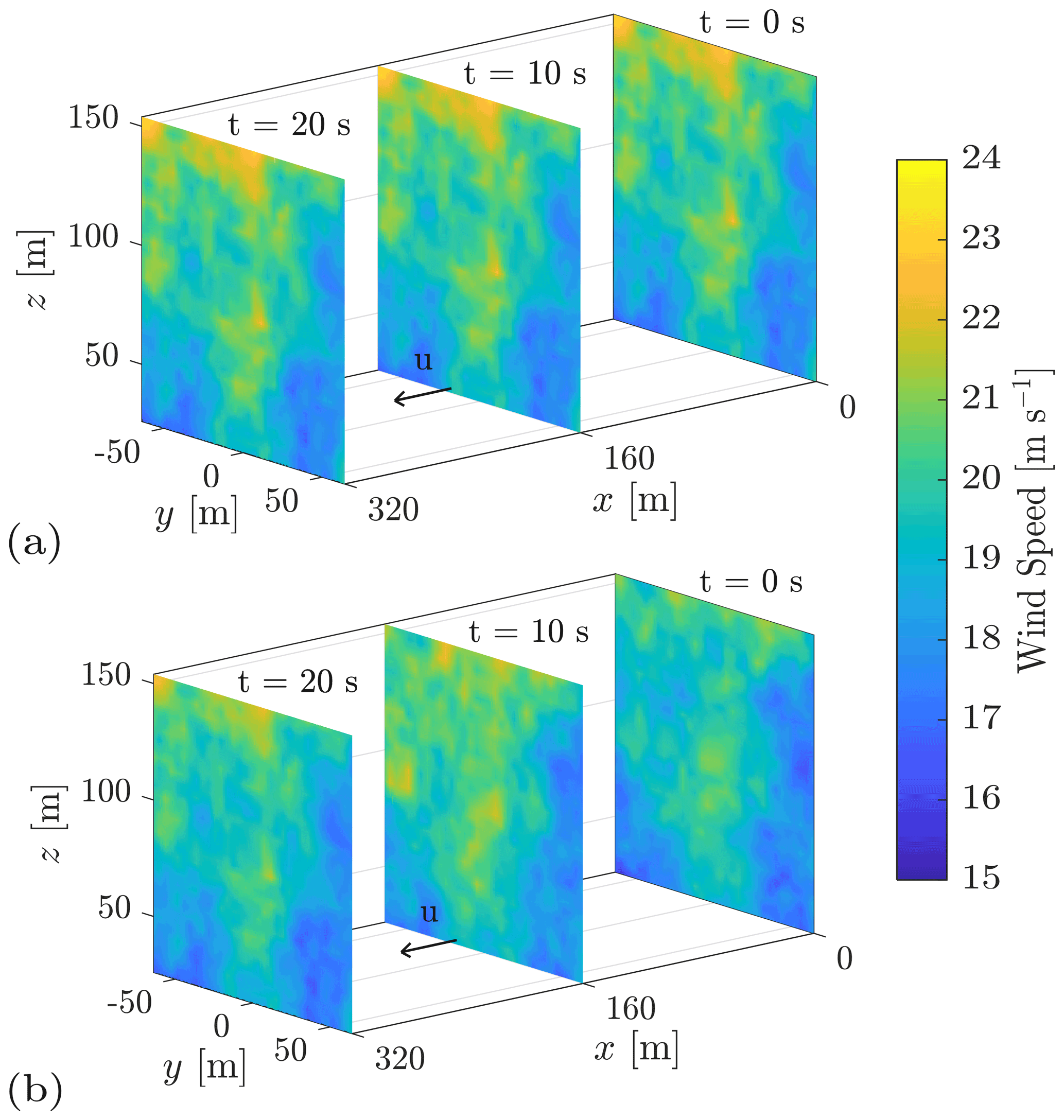
Figure 1 (a) A frozen turbulent wind field generated with the Mann turbulence generator. (b) An unfrozen turbulent wind field generated with the open-access tool evoTurb by combining multiple wind fields from the Mann turbulence generator. The turbulence properties are as follows: mean wind speed = 16 m s⁻¹, turbulence intensity = 0.16, and shear exponent = 0.2. Only the U component is shown.

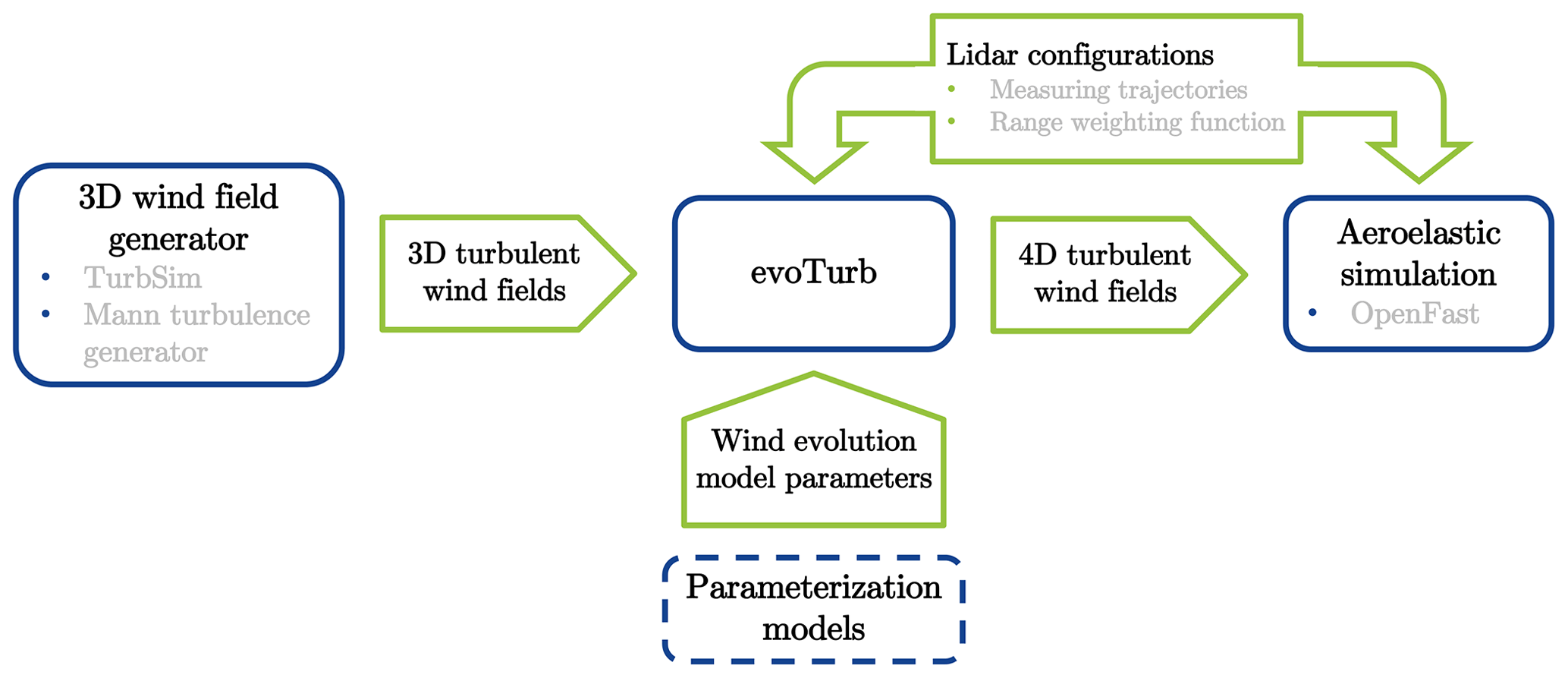
Figure 2 Concept for integrating the 4D wind field simulator evoTurb into the aeroelastic simulation of wind turbines.

Since the 4D wind field simulation is supposed to be applied in combination with lidar simulations, it is expected to generate wind speed time series for a 3D grid, and thus the computational effort is much larger than that of the 3D method. Therefore, we further look into the possibility to reduce the size of the simulation grid. For LAC, the auto-spectrum of line-of-sight (LOS) measurements is an important indicator since it is related to its variance in the time domain, which can be further used to estimate turbulence intensity (Peña et al., 2017; Schlipf et al., 2020). In addition, the coherence between the lidar-estimated u component in the upstream wind by a nacelle-mounted lidar and the u component on the rotor plane can be used to derive the usable frequency components of lidar signals for the feed-forward control (Schlipf, 2015). Hence, we focus on the impact of spatial discretization in lidar simulations on these two quantities. In this work, we analyze the discretization of a lidar range weighting function, different interpolation methods of wind speeds, and different simulation grids to provide some insights to optimize the simulation configurations.

This paper is organized as follows: Sect. 2 explains the methodology of the 4D wind field simulation, Sect. 3 discusses lidar simulations based on 4D wind fields, and Sect. 4 gives a summary and an outlook of this research.

2 Four-dimensional wind field generation

This section focuses on the methodology and implementation of the 4D wind field generation method proposed in this research. Section 2.1 introduces the basic approach of the Veers method for the 3D wind field generation. Section 2.2 explains how the Veers method can be extended to 4D. Section 2.3 proposes a two-step Cholesky decomposition approach to make the 4D wind field generation more feasible in practice. Section 2.4 shows the implementation of the 4D wind field generation coupling with TurbSim and MTG. Section 2.5 gives the validation of the proposed 4D wind field generation method.

2.1 The Veers method for 3D wind field generation

The Veers method (Veers, 1988) is based on the generation of random processes, which generates 3D turbulent wind fields by the complex Fourier coefficients (CFCs) in the frequency domain. To maintain required coherence among the turbulence, for each frequency component, a coherence matrix that contains the magnitude coherence between any two wind speed fluctuations at this frequency is factorized using the Cholesky decomposition (Press et al., 2007) and multiplied by uniformly distributed random phases to form a transformation matrix. This matrix is then scaled by a factor proportional to the square root of the auto-spectrum at this frequency to obtain the CFCs for this frequency component. This procedure is conducted for the whole frequency range to acquire the CFCs for all frequency components, and the time series of wind speed fluctuations are generated by applying inverse fast Fourier transform (IFFT) (Heideman et al., 1985) to the CFCs.

As explained above, the key to the Veers method is to compute the CFCs for each frequency component. Here, we take the example of generating time series of the u component to explain the key formula in detail. The reason for taking the u component as an example is that currently only the longitudinal coherence of the u component is considered to be introduced in wind field generation.

Consider n non-overlapping spatial points on the yz plane, which can be arbitrarily distributed. For a specific frequency component (the frequency is omitted in the following formulas for brevity), the CFC vector of the u component for 3D wind fields is computed by (Veers, 1988)

$$\begin{array}{}\text{(1)}& {\mathbf{U}}_{yz}=[{\widehat{u}}_{yz,\mathrm{1}}{\widehat{u}}_{yz,\mathrm{2}}\mathrm{\cdots }{\widehat{u}}_{yz,n}{]}^{\top }=A_u{\mathbf{H}}_{u,yz}{\mathbf{X}}_n.\end{array}$$

This formula consists of three parts.

• A_u is the two-sided Fourier coefficient obtained from the auto-spectrum of the u component S_u at this frequency,

  $$\begin{array}{}\text{(2)}& A_u=\sqrt{\mathrm{\Delta }f\cdot S_u},\end{array}$$

  with Δf the frequency step in Hz. A factor of $\mathrm{1}/\mathrm{2}$ needs to be multiplied in the square root if S_u is a one-sided power spectral density. For a specific frequency component, A_u is a constant.

• H_u,yz is the Cholesky factor obtained by factorizing the lateral–vertical coherence matrix C_u,yz at this frequency using Cholesky decomposition. C_u,yz is a n-by-n matrix with entries ${\mathit{\gamma }}_{u,yz,i,j}$ the magnitude coherence of the u component between any two spatially separated points indexed with i and j on the yz plane:

  $$\begin{array}{}\text{(3)}& {\mathbf{C}}_{u,yz}=\left[\begin{array}{ccc}{\mathit{\gamma }}_{u,yz,\mathrm{1},\mathrm{1}}& \mathrm{\dots }& {\mathit{\gamma }}_{u,yz,\mathrm{1},n}\\ \mathrm{⋮}& \mathrm{\ddots }& \mathrm{⋮}\\ {\mathit{\gamma }}_{u,yz,n,\mathrm{1}}& \mathrm{\dots }& {\mathit{\gamma }}_{u,yz,n,n}\end{array}\right].\end{array}$$

  For the general definition of the spatial coherence, please refer to Appendix A. Because under the same wind field conditions, ${\mathit{\gamma }}_{u,yz,i,j}$ only depends on the spatial separation between the two points (see Eq. A3), C_u,yz is a symmetric matrix. The Cholesky decomposition can decompose a real, symmetric, positive-definite matrix into the product of a lower triangular matrix, i.e., the Cholesky factor, and its transpose. For brevity, the operation to obtain the Cholesky factor is denoted by “chol( )”. In this case,

  $$\begin{array}{}\text{(4)}& {\mathbf{H}}_{u,yz}=\text{chol}\left({\mathbf{C}}_{u,yz}\right),\end{array}$$

  with

  $$\begin{array}{}\text{(5)}& {\mathbf{H}}_{u,yz}=\left[\begin{array}{ccc}{h}_{u,yz,\mathrm{1},\mathrm{1}}& & \mathrm{0}\\ \mathrm{⋮}& \mathrm{\ddots }& \\ h_{u,yz,n,\mathrm{1}}& \mathrm{\cdots }& h_{u,yz,n,n}\end{array}\right],\end{array}$$

  which satisfies

  $$\begin{array}{}\text{(6)}& {\mathbf{C}}_{u,yz}={\mathbf{H}}_{u,yz}{\mathbf{H}}_{u,yz}^{\top }.\end{array}$$
• (3)

  X_n is a n-by-1 vector of random phases which are uniformly distributed between 0 and 2π,

  $$\begin{array}{}\text{(7)}& {\mathbf{X}}_n=[e^{\mathbf{i}{\mathit{\theta }}_{\mathrm{1}}}{e}^{\mathbf{i}{\mathit{\theta }}_{\mathrm{2}}}\mathrm{\cdots }{e}^{\mathbf{i}{\mathit{\theta }}_n}{]}^{\top },\end{array}$$

  with i the imaginary unit. For convenience, the size of the vector is indicated by the subscript.

2.2 Extending the Veers method for 4D wind generation

In principle, Eq. (1) can be used to generate random processes with specific correlation according to the given coherence matrix, which is not limited by dimensions. Therefore, we can extend Eq. (1), which is originally for spatial points on a vertical plane corresponding to 3D wind fields $\mathbf{V}(t,y,z)$, to spatial points in 3D space corresponding to 4D wind fields $\mathbf{V}(t,x,y,z)$.

To explain this idea, we continue with the example of the u component. Consider p non-overlapping spatial points in 3D space, which can also be arbitrarily distributed as in the 3D case. For a specific frequency component, the CFC vector of the u component for 4D wind fields can be formulated in a similar way to Eq. (1)

$$\begin{array}{}\text{(8)}& {\mathbf{U}}_{xyz}=A_u{\mathbf{H}}_{u,xyz}{\mathbf{X}}_p,\end{array}$$

with

$$\begin{array}{}\text{(9)}& {\mathbf{H}}_{u,xyz}=\text{chol}\left({\mathbf{C}}_{u,xyz}\right).\end{array}$$

In Eq. (8), A_u is the same as that in Eq. (1). X_p is still a vector of random phases but with a size of p-by-1 according to the grid size. The main difference lies in the Cholesky factor for 4D wind fields H_u,xyz (p-by-p) or, more precisely, the 3D coherence matrix C_u,xyz (p-by-p), which is supposed to contain the magnitude coherence of the u component between any two spatial points in 3D space ${\mathit{\gamma }}_{u,xyz,i,j}$.

Currently, there is no simple model for the 3D coherence available. Therefore, a general approach to create the 3D coherence is combining the lateral–vertical coherence and the longitudinal coherence (see, e.g., Schlipf et al., 2013; Laks et al., 2013; Bossanyi et al., 2014; Simley, 2015). Simley (2015) investigated two different methods for combining the lateral–vertical and the longitudinal coherence, i.e., the product method, taking the product of both, and the root-of-sum-of-squares (RSS) method, taking the RSS of both. According to the comparison based on LESs, the RSS method is more accurate, while the product method slightly underestimates the 3D coherence (Simley, 2015). However, we choose the product method in this study because it allows us to come up with a two-step Cholesky decomposition approach which makes the 4D wind field generation more feasible in practice. This will be introduced in Sect. 2.3.

In fact, Eq. (8) is exactly the general formula of the CFCs in the 4D wind field generation. After acquiring the CFCs, the subsequent steps are the same as in the 3D case. Finally, the generated wind speeds should be time-shifted according to the mean wind speed and the corresponding longitudinal positions. It is worth mentioning that compared to the methods proposed by Laks et al. (2013) or Bossanyi (2013), which only extend the Veers method from the wind field at the rotor position to an additional vertical plane, the method proposed here is a more general extension of the Veers method and thus more widely applicable.

2.3 Two-step Cholesky decomposition approach

A problem may occur when directly applying Eq. (8). The size of the 3D coherence matrix could be much larger than the size of the lateral–vertical coherence matrix (i.e., p≫n) because the former considers one more spatial dimension than the latter. This will lead to a much higher computational cost of the Cholesky decomposition, which is theoretically proportional to the cube of the matrix size, denoted as O(p³) (Higham, 2008). To tackle this issue, we propose a two-step Cholesky decomposition approach by taking the following two assumptions.

1. As mentioned above, the 3D coherence ${\mathit{\gamma }}_{u,xyz,i,j}$ is assumed to be the product of the lateral–vertical coherence ${\mathit{\gamma }}_{u,yz,i,j}$ and the longitudinal coherence ${\mathit{\gamma }}_{u,x,i,j}$:

   $$\begin{array}{}\text{(10)}& {\mathit{\gamma }}_{u,xyz,i,j}={\mathit{\gamma }}_{u,yz,i,j}{\mathit{\gamma }}_{u,x,i,j}.\end{array}$$

2. Considering that regular grids are more commonly used in practice, we define a 3D grid with m identical, non-overlapping planes perpendicular to the x axis with n points (i.e., p=mn) instead of an arbitrary grid.

Similar to the lateral–vertical coherence, the longitudinal coherence only depends on the spatial separation between the two points on the x axis under the same wind field conditions. Therefore, for these m planes, a longitudinal coherence matrix C_u,x can be formed by the magnitude coherence of the u component between any two planes:

$$\begin{array}{}\text{(11)}& {\mathbf{C}}_{u,x}=\left[\begin{array}{ccc}{\mathit{\gamma }}_{u,x,\mathrm{1},\mathrm{1}}& \mathrm{\dots }& {\mathit{\gamma }}_{u,x,\mathrm{1},m}\\ \mathrm{⋮}& \mathrm{\ddots }& \mathrm{⋮}\\ {\mathit{\gamma }}_{u,x,m,\mathrm{1}}& \mathrm{\dots }& {\mathit{\gamma }}_{u,x,m,m}\end{array}\right].\end{array}$$

With the two assumptions, the 3D coherence matrix C_u,xyz (mn-by-mn) can be computed by the Kronecker product “⊗” (Henderson et al., 1983) of the longitudinal coherence matrix C_u,x (m-by-m) and the lateral–vertical coherence matrix C_u,yz (n-by-n):

$$\begin{array}{}\text{(12)}& \begin{array}{rl}{\mathbf{C}}_{u,xyz}& ={\mathbf{C}}_{u,x}\otimes {\mathbf{C}}_{u,yz}\\ & =\left[\begin{array}{ccc}{\mathit{\gamma }}_{u,x,\mathrm{1},\mathrm{1}}{\mathbf{C}}_{u,yz}& \mathrm{\dots }& {\mathit{\gamma }}_{u,x,\mathrm{1},m}{\mathbf{C}}_{u,yz}\\ \mathrm{⋮}& \mathrm{\ddots }& \mathrm{⋮}\\ {\mathit{\gamma }}_{u,x,m,\mathrm{1}}{\mathbf{C}}_{u,yz}& \mathrm{\dots }& {\mathit{\gamma }}_{u,x,m,m}{\mathbf{C}}_{u,yz}\end{array}\right].\end{array}\end{array}$$

With the help of the Kronecker product, we derived a very useful property for the Cholesky decomposition:

$$\begin{array}{}\text{(13)}& \text{chol}(\mathbf{A}\otimes \mathbf{B})=\text{chol}\left(\mathbf{A}\right)\otimes \text{chol}\left(\mathbf{B}\right),\end{array}$$

with A and B matrices of arbitrary size. The mathematical proof is given in Appendix C. Applying Eq. (13), Eq. (9) becomes

$$\begin{array}{}\text{(14)}& \begin{array}{rl}{\mathbf{H}}_{u,xyz}& =\text{chol}\left({\mathbf{C}}_{u,xyz}\right)\\ & =\text{chol}({\mathbf{C}}_{u,x}\otimes {\mathbf{C}}_{u,yz})\\ & =\text{chol}\left({\mathbf{C}}_{u,x}\right)\otimes \text{chol}\left({\mathbf{C}}_{u,yz}\right)\\ & ={\mathbf{H}}_{u,x}\otimes {\mathbf{H}}_{u,yz},\end{array}\end{array}$$

which means instead of applying the Cholesky decomposition to a large matrix, we can now break it down into two Cholesky decomposition for two small matrices. We call this two-step Cholesky decomposition. This approach can reduce the computational time of Cholesky decomposition from O((mn)³) to O(m³)+O(n³).

With the two-step Cholesky decomposition, Eq. (8) is rewritten as

$$\begin{array}{}\text{(15)}& {\mathbf{U}}_{xyz}=A_u({\mathbf{H}}_{u,x}\otimes {\mathbf{H}}_{u,yz}){\mathbf{X}}_{mn}.\end{array}$$

Compared to Eq. (1), only the Cholesky factor of the longitudinal coherence matrix H_u,x is a new term, and the other terms can be obtained from 3D wind fields. This leads to the idea to generate a 4D wind field by combining multiple statistically independent 3D wind fields.

2.4 Four-dimensional wind field generator: evoTurb

Following the idea mentioned above, Eq. (15) can be rearranged as

$$\begin{array}{}\text{(16)}& {\mathbf{U}}_{xyz}=({\mathbf{H}}_{u,x}\otimes A_u{\mathbf{H}}_{u,yz})\left[\begin{array}{c}{\mathbf{X}}_{n,\mathrm{1}}\\ \mathrm{⋮}\\ {\mathbf{X}}_{n,m}\end{array}\right].\end{array}$$

It can be observed that the term $A_u{\mathbf{H}}_{u,yz}{\mathbf{X}}_{n,i}$ is exactly the CFC vector of the u component for a 3D wind field (see Eq. (1). Instead of directly calculating U_yz,i, it can be obtained by applying fast Fourier transformation (FFT; denoted by ℱ{ }) to a time series of the u component ${\mathbf{u}}_{yz,i}(t,y,z)$ generated with a 3D wind field generator

$$\begin{array}{}\text{(17)}& A_u{\mathbf{H}}_{u,yz}{\mathbf{X}}_{n,i}={\mathbf{U}}_{yz,i}=\mathcal{F}\mathit{\left\{}{\mathbf{u}}_{yz,i}\right(t,y,z\left)\mathit{\right\}}.\end{array}$$

Based on this, the CFCs of the u component for a 4D wind field with m vertical planes can be calculated by constraining m statistically independent 3D wind fields with the longitudinal coherence matrix,

$$\begin{array}{}\text{(18)}& \left[\begin{array}{c}{\mathbf{U}}_{xyz,\mathrm{1}}^{\top }\\ \mathrm{⋮}\\ {\mathbf{U}}_{xyz,m}^{\top }\end{array}\right]={\mathbf{H}}_{u,x}\left[\begin{array}{c}{\mathbf{U}}_{yz,\mathrm{1}}^{\top }\\ \mathrm{⋮}\\ {\mathbf{U}}_{yz,m}^{\top }\end{array}\right],\end{array}$$

with U_xyz,i the CFC vector (n-by-1) of the u component of the ith yz plane in the 4D wind field and U_yz,i the CFC vector (n-by-1) of the u component of the ith 3D wind field. And thus the CFC matrix of the 4D wind field (left-hand side) and the CFC matrix of the 3D wind fields (second term of the right-hand side) are m-by-n matrices. It is essential to ensure that all the random phases within the CFC matrix of the 3D wind fields follow a uniform distribution. This is why it is emphasized that the input 3D wind fields must be “statistically independent”; i.e., they must be generated with different random seeds.

In comparison to the direct generation of 4D wind fields, the advantage of this concept is that it can introduce the longitudinal coherence into the stochastic wind field generation without changing any other wind field properties generated by these standard tools. This is conducive to the integration of the 4D wind field generation with the current framework of the aeroelastic simulation of wind turbines. Moreover, this concept makes it possible to use pre-generated 3D wind fields (with different random seeds) for the generation of 4D wind fields. The input 3D wind fields should be randomly selected and non-repetitive. Different combinations of the same 3D wind fields, i.e., assigning the 3D wind fields to the vertical planes in a 4D wind field differently, can form different 4D wind fields, and thus a 3D wind field can be used multiple times. This can significantly reduce the computational effort required to generate 4D wind fields, considering that in the aeroelastic simulations of wind turbines, a design load case requires several simulations using wind fields generated with different random seeds (DNV, 2016).

Based on this concept, we developed an open-access 4D wind field generator – evoTurb (GitHub: https://github.com/SWE-UniStuttgart/evoTurb, last access: 2 March 2022). As illustrated in Fig. 2, evoTurb is coupled with TurbSim (specifically for the Kaimal model Kaimal et al., 1972) and MTG, but the implementation of both is slightly different. For more details regarding the turbulence models, please refer to Appendix A.

For the Kaimal model in TurbSim, we just need to apply Eq. (18) to the u component because the Kaimal model only considers the spatial coherence of the u component. The v and w components of the 4D wind field can be directly taken from the corresponding 3D wind fields. However, in reality, the atmospheric air flow is assumed incompressible for normal wind turbine applications. This implies that either the v or w component is spatially correlated due to the continuity of the incompressible fluid as discussed by Mann (1994).

The Mann model (Mann, 1994) additionally contains the coherence between the u and w components. If we only apply Eq. (18) to the u component, the coherence between the u and w components will be decorrelated except for the first vertical plane. To maintain the coherence between the u and w components defined by the Mann model, we assume that the w component also follows the same longitudinal coherence as that of the u component

$$\begin{array}{}\text{(19)}& {\mathbf{H}}_{w,x}={\mathbf{H}}_{u,x}.\end{array}$$

Similar to Eq. (18), the CFC matrix of the w component is calculated with

$$\begin{array}{}\text{(20)}& \left[\begin{array}{c}{\mathbf{W}}_{xyz,\mathrm{1}}^{\top }\\ \mathrm{⋮}\\ {\mathbf{W}}_{xyz,m}^{\top }\end{array}\right]={\mathbf{H}}_{w,x}\left[\begin{array}{c}{\mathbf{W}}_{yz,\mathrm{1}}^{\top }\\ \mathrm{⋮}\\ {\mathbf{W}}_{yz,m}^{\top }\end{array}\right],\end{array}$$

with

$$\begin{array}{}\text{(21)}& {\mathbf{W}}_{yz,i}=\mathcal{F}\mathit{\left\{}{\mathbf{w}}_i\right(t,y,z\left)\mathit{\right\}}.\end{array}$$

The functionality of evoTurb (referred to the main script of the codes) is briefly introduced as follows.

1. TurbConfig. Import the configuration file.

2. Execute3DSim. Call TurbSim or MTG to generate m 3D wind fields with different random seeds and save these wind fields for later use. If the same wind fields already exist, this step will be skipped.

3. Import3DTurb. Import the generated 3D wind fields.

4. Generate4DTurb. Compute the CFCs of the 3D wind fields. Compute the longitudinal coherence matrices using a wind evolution model and the corresponding Cholesky factors. Compute the CFCs of the 4D wind field. Apply IFFT to the CFCs of the 4D wind field.

5. Export4DTurb. Export the 4D wind field as binary files.

The wind evolution models supported by evoTurb are briefly introduced in Appendix B.

In fact, the Mann model additionally contains the spatial coherence of v at different locations, the spatial coherence of w components at different locations, and the coherence between the u and w components at the same position, which theoretically should also be considered in the 4D wind field simulation. de Maré and Mann (2016) and Bos (2017) have proposed methods to extend the Mann model to the spatial–temporal tensor, from which the longitudinal coherence of all velocity components can be derived. However, the model proposed by de Maré and Mann (2016) has not yet been validated with measurements. And Bos's approach (Bos, 2017) requires a formula of the wavenumber-dependent eddy lifetimes, which still need to be investigated with experiments or high-fidelity CFD simulations. Because the longitudinal coherence of the v and w component is less important for LAC compared to that of the u component (Schlipf et al., 2013; Held and Mann, 2019), we put our emphasis only on the u component in this study. The effects of neglecting the longitudinal coherence of the v component and the rationality of assuming the identical longitudinal coherence for the u and w components remain to be investigated.

2.5 Validation of evoTurb

The validation of evoTurb mainly focuses on two aspects: whether the longitudinal coherence is correctly simulated and whether other wind field properties generated by TurbSim and MTG are not affected by evoTurb.

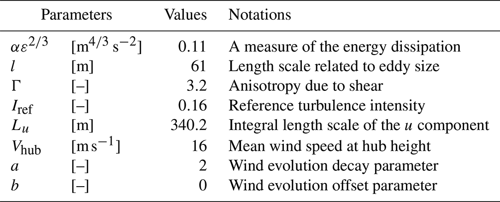
The validation is done by two examples coupling with TurbSim and MTG, respectively. The relevant parameters of the 4D wind field generation are summarized in Table 1. The Mann model parameters are defined according to Mann (1994). For simplicity, the wind evolution model of Simley and Pao (2015) (see Table B1) is applied with user-defined parameters instead of its parameterization model, and the parameters are chosen based on Chen et al. (2021). For the validation of coherence and spectra, we consider the spectrum calculated from one realization (one simulated time series) as one sample and compute the ensemble average of 16 samples generated with different random seeds. It is worth mentioning that the averaged coherence is calculated by dividing the averaged cross-spectrum by the averaged auto-spectra. The auto-spectra and cross-spectra are estimated using the Bartlett's averaged periodogram method (Bartlett, 1948) with rectangular windows (size of 1024 data points).

Table 1 The wind field parameters for the validation. $\mathit{\alpha }{\mathit{\epsilon }}^{\mathrm{2}/\mathrm{3}}$, l, and Γ are the Mann model parameters. I_ref and L_u are parameters of the IEC Kaimal model (turbulence class A). And the rest are the common parameters of both models. The hub height is considered 90 m.

To validate the coherence, Fig. 3 compares the theoretical and simulated coherence between different horizontal separations in the two 4D wind fields. The good agreement between the theoretical and simulated longitudinal coherence of Δx=50 m and Δx=100 m, respectively, proves that evoTurb can correctly model the user-defined longitudinal coherence in 4D wind fields. The fact that the lateral–vertical coherence of Δy=20 m is consistent with its theoretical curve confirms that the original turbulence characteristics of both tools are not changed by evoTurb. The good match between the theoretical and simulated 3D coherence of Δx=50 m and Δy=20 m validates that the longitudinal coherence and the lateral–vertical coherence are correctly combined in evoTurb.

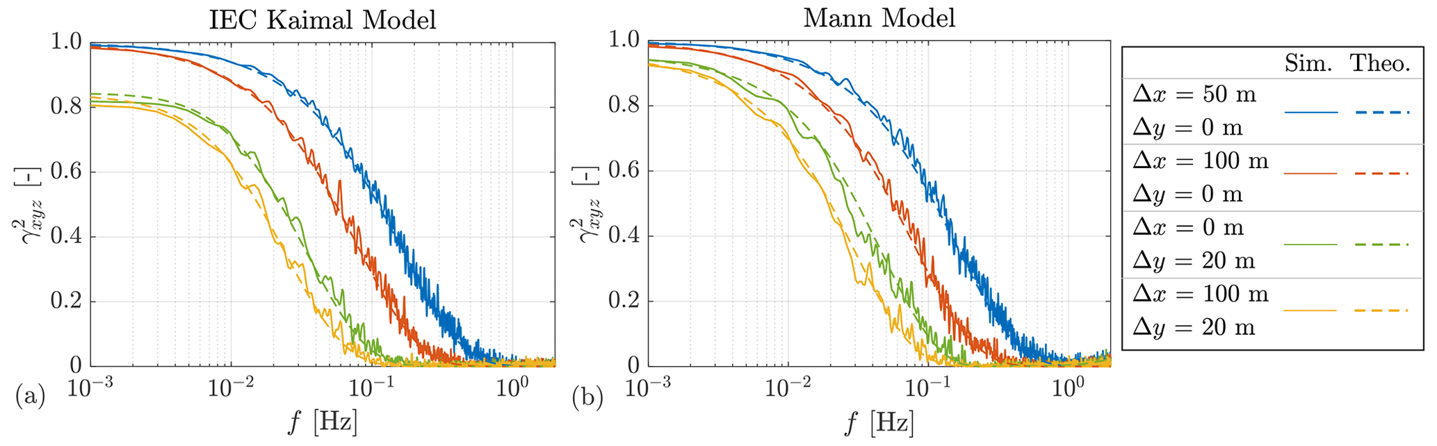
Figure 3 Comparison of the theoretical and simulated coherence between different horizontal separations in 4D wind fields. The simulated coherence is calculated by dividing the averaged cross-spectra by the auto-spectra of 16 samples. Sim.: simulated. Theo.: theoretical.

As presented in Sect. 2.4, evoTurb generates a 4D wind field by constraining independent 3D wind fields with the user-defined longitudinal coherence. This process is visualized in Fig. 4 by the example of MTG. Figure 4a–c show three independent 3D wind fields generated with MTG. Obviously, there is no coherence between them. These three wind fields are fed in evoTurb, specifically as the vertical planes at x=0 m, x=50 m, and x=100 m, respectively, in this example. It can be observed in Fig. 4d–f that after applying the longitudinal coherence, the three wind fields become coherent, especially the large eddy structures that correspond to the low-frequency components. More specifically, Fig. 4a and d are identical since the wind field at x=0 m is inherently regarded as the reference wind field in the constraining process; the wind fields in Fig. 4e and f are generated by constraining the wind fields in Fig. 4b and c to Fig. 4a with the coherence at Δx=50 m and Δx=100 m at the same time. Because the smaller the longitudinal separation, the higher the coherence, Fig. 4e is more similar to Fig. 4a compared to Fig. 4f, whereas Fig. 4f retains more eddy structures of the original wind field in Fig. 4c, e.g., the strong eddies at z of 100 to 150 m in the first 10 s. Please note that the temporal shifts due to the longitudinal separations are not shown in Fig. 4d–f in order to make it easier to observe the difference caused only by wind evolution.

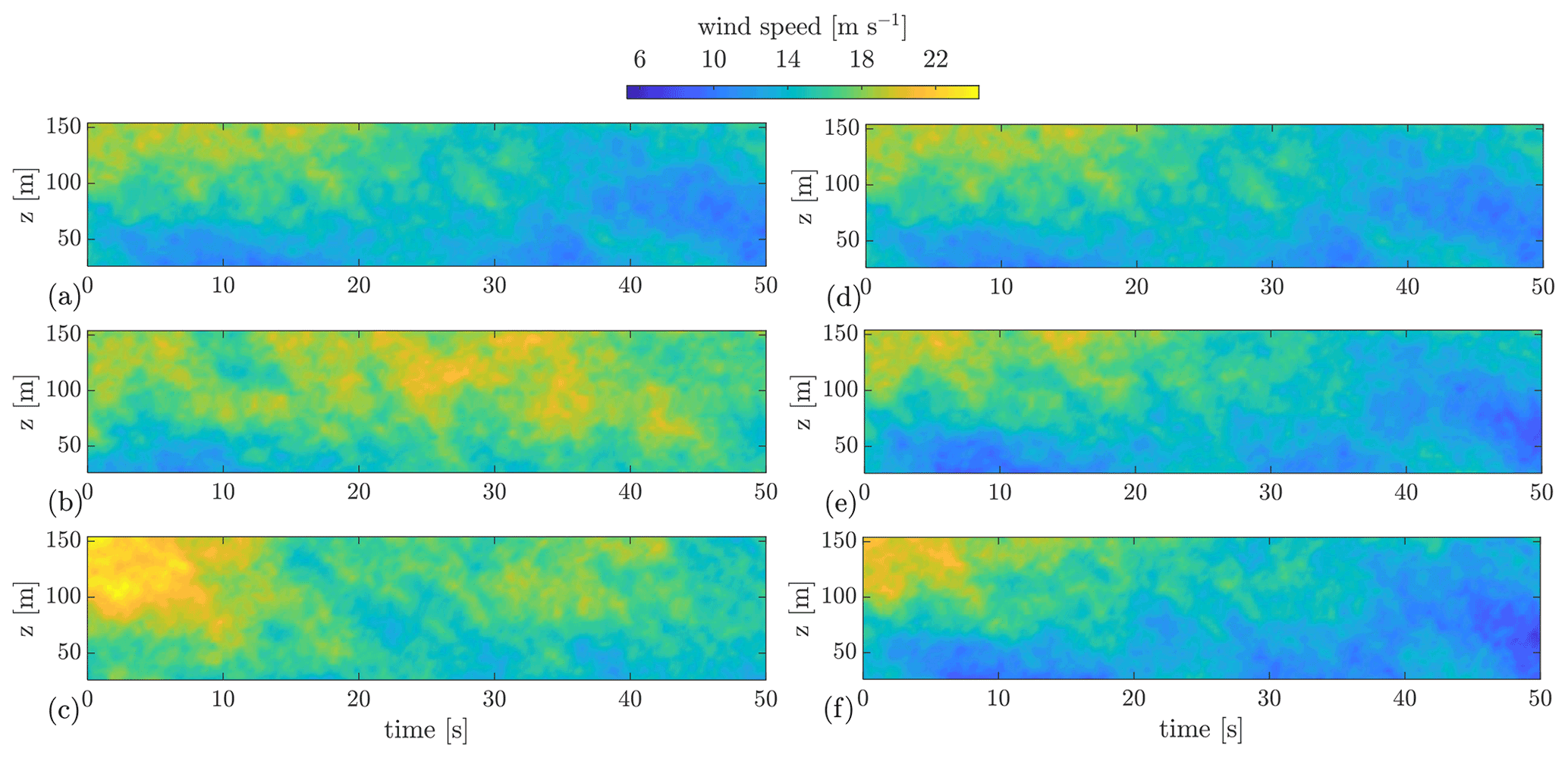
Figure 4 Illustration of the U component in a 4D wind field. Panels (a)–(c) are three independent realizations of 3D turbulent wind fields generated with the Mann turbulence generator, which are fed into evoTurb. Panels (d)–(f) are the corresponding vertical planes at x=0 m, x=50 m, and x=100 m in the 4D wind field. The temporal shifts due to the longitudinal separations are not shown.

Regarding the special issue related to the Mann model raised in Sect. 2.4, Fig. 5 specifically illustrates the auto-spectra of u, v, and w components and the uw cross-spectrum at x=100 m of the example of MTG. The good agreement between the simulated spectra and the theoretical ones derived from the Mann (1994) spectral tensor proves that with the assumption made in Sect. 2.4, the auto-spectra and the uw cross-spectra are maintained in the constraining process. In addition, it can be observed in Fig. 4 that the anisotropy turbulence due to the shear distortion considered in the Mann model also remains unaffected.

Figure 5 Comparison of the simulated and theoretical spectra of the Mann model at x=100 m in a 4D wind field. The simulated spectra are averaged with 16 samples.

3 Lidar simulation with integration of 4D wind fields

As mentioned in the introduction, 4D wind field generation is supposed to be applied to the simulation of lidar-assisted control systems, and thus this section intends to study its integration with lidar simulations. Section 3.1 briefly introduces the basics of lidar simulations. Section 3.2 derives the theoretical formulas of the auto-spectrum of LOS measurements and the coherence between the rotor effective wind speed (REWS) and the lidar-estimated REWS to serve as a theoretical basis. Section 3.3 investigates the effect of the discretization of a lidar range weighting function on the simulated auto-spectrum of LOS measurements. Section 3.4 discusses the impact of interpolation methods on the auto-spectrum of the u component in lidar simulations. Section 3.5 discusses impact of discrete simulations on lidar spectral properties and proposes a sparse grid for lidar simulations to reduce the computational effort of 4D wind field generation.

3.1 Lidar simulation

Lidars in this article refer specifically to coherent Doppler wind lidars whose measuring principle is based on the optical Doppler effect. Such lidar systems measure wind speed by transmitting narrow bandwidth laser signals into the atmosphere and detecting the Doppler shift in the backscattered signals from aerosol particles in the atmosphere using coherent detection (Fujii and Fukuchi, 2005). The Doppler shift is caused by the motion of the aerosol particles entrained with the wind and thus can be used to estimate the line-of-sight wind speed (i.e., the projection of wind velocities onto the laser beam direction) in the probe volumes of lidars. To extract the Doppler shift, the collected backscattered signals are converted into digital signals and split into blocks, on which FFT is performed to calculate their power spectra. These spectra are averaged to reduce background noises so that the frequency of the peak can be estimated.

Two types of wind lidars are commonly available for the wind energy applications: continuous-wave lidars and pulsed lidars. In this research, we take the example of a pulsed lidar. As its name implies, a pulsed lidar emits regularly spaced short laser pulses. In the data processing of pulsed lidars, the return signals of each pulse are first divided into range gates, and the averaging of power spectra is done for the same range gate from different pulses (Peña et al., 2013).

Due to the measuring principle of lidars, two effects should be considered in lidar simulations in general: the volume averaging effect and the time averaging effect (Schlipf, 2015). As mentioned above, this section aims to study the impact of spatial discretization in lidar simulations. Therefore, the focus of our discussion here is on the volume averaging effect rather than the time averaging effect, and thus the simulation of the time averaging effect is omitted by generating the 4D wind fields with the same sampling rate as the lidar simulation (f_s=4 Hz).

The volume averaging effect can be simulated by applying a range weighting function φ(s) to the ideal point measurements of the LOS wind speeds v_losP(r,t) at the measuring distance r within the probe volume (see, e.g., Peña et al., 2013, 2017):

$$\begin{array}{}\text{(22)}& v_{\mathrm{los}}(r_{\mathrm{0}},t)=\underset{-\mathrm{\infty }}{\overset{\mathrm{\infty }}{\int }}\mathit{\phi }\left(s\right)v_{\mathrm{losP}}(r,t)\mathrm{d}s\mathrm{with}s=r-r_{\mathrm{0}},\end{array}$$

where v_los(r₀,t) is the LOS wind speed of the probe volume focusing at the distance r₀, s is the spatial distance to the focus point along the laser beam, and t is time. v_losP(r,t) is calculated by projecting the vector of the wind speed at r onto the laser beam direction:

$$\begin{array}{}\text{(23)}& v_{\mathrm{losP}}(r,t)=\left[u\right(r,t\left)v\right(r,t\left)w\right(r,t\left)\right]\cdot [x_{\mathrm{n}}{y}_{\mathrm{n}}{z}_{\mathrm{n}}{]}^{\top },\end{array}$$

with [x_n y_n z_n] the normal vector of the beam direction (PO in Fig. 6). The normal vector can be simply calculated after knowing the azimuth angle ϕ and elevation angle β of the lidar beam. Figure 6 shows a typical coordinate system used for simulating an upstream-looking nacelle lidar.

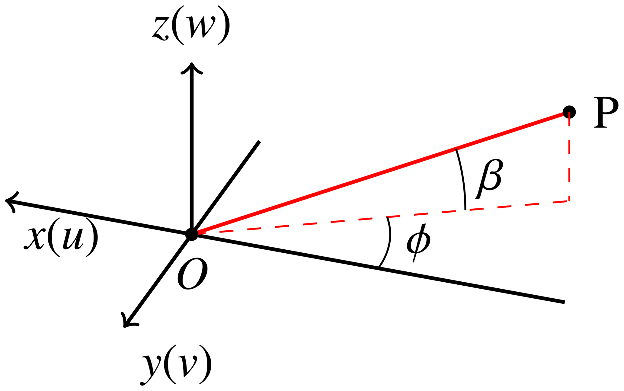
Figure 6 The typical coordinate system for simulating an upstream-looking nacelle lidar. P denotes an arbitrary point along the lidar beam direction.

For pulsed lidars, the range weighting function can be analytically computed as the convolution between the pulse power profile and the range gate profile (Banakh and Smalikho, 1994), which is approximately constant for different range gates (Cariou, 2013). For simplicity, the range weighting function is modeled by a Gaussian-shape function (see, e.g., Schlipf, 2015):

$$\begin{array}{}\text{(24)}& \mathit{\phi }\left(s\right)={\displaystyle \frac{\mathrm{1}}{{\mathit{\sigma }}_{\mathrm{L}}\sqrt{\mathrm{2}\mathit{\pi }}}}\exp \left(-{\displaystyle \frac{s^{\mathrm{2}}}{\mathrm{2}{\mathit{\sigma }}_{\mathrm{L}}^{\mathrm{2}}}}\right)\mathrm{with}{\mathit{\sigma }}_{\mathrm{L}}={\displaystyle \frac{W_{\mathrm{L}}}{\mathrm{2}\sqrt{\mathrm{2}\ln \mathrm{2}}}},\end{array}$$

where the full width at half maximum W_L is set to 30 m following Cariou (2013).

In lidar simulations, Eq. (22) requires a discrete approximation in practice:

$$\begin{array}{}\text{(25)}& v_{\mathrm{los}}(r_{\mathrm{0}},t)=\sum _{k=\mathrm{1}}^{N_{\mathrm{rw}}}{F}_{\mathrm{rw},k}\cdot v_{\mathrm{losP},k}(r_k,t),\end{array}$$

with the number of discrete points N_rw and the discrete range weighting coefficient F_rw,k for the spatial point indexed with k defined as

$$\begin{array}{}\text{(26)}& F_{\mathrm{rw},k}={\displaystyle \frac{\mathit{\phi }\left(s_k\right)}{{\sum }_{k=\mathrm{1}}^{N_{\mathrm{rw}}}\mathit{\phi }\left(s_k\right)}}.\end{array}$$

The discrete range weighting coefficients are normalized to ensure that their sum equals one. In general, equidistant discrete points are selected.

3.2 Derivation of auto-spectrum and coherence of lidar measurements

In this section, we derive the analytical expressions of the auto-spectrum of LOS measurements and the coherence between the REWS and the lidar-estimated REWS to serve as a theoretical basis for the analysis of the impact of spatial discretization in lidar simulations in Sect. 3.3–3.5.

We formulate the mathematical derivation according to the Kaimal model and perform the derivation mainly based on the linearity of 1D Fourier transform because this procedure is easier to understand. As for the Mann model, Mann et al. (2008) and Held and Mann (2019) give neat derivations for the auto-spectrum of LOS measurements and the cross-spectrum of the lidar-estimated and the actual rotor effective wind speeds based on the Mann spectral tensor based on the multiple integral and the multidimensional Fourier transform. Following similar approaches, the lidar spectral properties derived below can also be conducted for the Mann model.

Inspired by Schlipf (2015), the theoretical auto-spectrum of LOS measurements is calculated by

$$\begin{array}{}\text{(27)}& S_{\mathrm{los}}=\mathcal{F}\mathit{\left\{}{v}_{\mathrm{los}}\mathit{\right\}}{\mathcal{F}}^{*}\mathit{\left\{}{v}_{\mathrm{los}}\mathit{\right\}},\end{array}$$

where ℱ^*{ } denotes the conjugate of Fourier transform. Taking the discrete approximation for the LOS measurements with N_rw points (see Eq. 25), Eq. (27) becomes

$$\begin{array}{}\text{(28)}& \begin{array}{rl}{S}_{\mathrm{los}}& =\mathcal{F}\mathit{\{}\sum _{i=\mathrm{1}}^{N_{\mathrm{rw}}}{F}_{\mathrm{rw},i}\cdot v_{\mathrm{losP},i}\mathit{\}}{\mathcal{F}}^{*}\mathit{\{}\sum _{j=\mathrm{1}}^{N_{\mathrm{rw}}}{F}_{\mathrm{rw},j}\cdot v_{\mathrm{losP},j}\mathit{\}}\\ & =\sum _{i=\mathrm{1}}^{N_{\mathrm{rw}}}\sum _{j=\mathrm{1}}^{N_{\mathrm{rw}}}{F}_{\mathrm{rw},i}{F}_{\mathrm{rw},j}\mathcal{F}\mathit{\left\{}{v}_{\mathrm{losP},i}\mathit{\right\}}{\mathcal{F}}^{*}\mathit{\left\{}{v}_{\mathrm{losP},j}\mathit{\right\}}\\ & =\sum _{i=\mathrm{1}}^{N_{\mathrm{rw}}}\sum _{j=\mathrm{1}}^{N_{\mathrm{rw}}}{F}_{\mathrm{rw},i}{F}_{\mathrm{rw},j}{S}_{\mathrm{losP},i,j}.\end{array}\end{array}$$

In Eq. (28), $S_{\mathrm{losP},i,j}$ denotes the cross-spectrum of two LOS wind speeds at the points i and j, which can be explicitly expanded by substituting Eq. (23) as follows (Schlipf, 2015):

$$\begin{array}{}\text{(29)}& \begin{array}{rl}{S}_{\mathrm{losP},i,j}& =\mathcal{F}\mathit{\{}{x}_{\mathrm{n}}{u}_i+y_{\mathrm{n}}{v}_i+z_{\mathrm{n}}{w}_i\mathit{\}}{\mathcal{F}}^{*}\mathit{\{}{x}_{\mathrm{n}}{u}_j+y_{\mathrm{n}}{v}_j+z_{\mathrm{n}}{w}_j\mathit{\}}\\ & =x_{\mathrm{n}}^{\mathrm{2}}{S}_{u,i,j}+x_{\mathrm{n}}{y}_{\mathrm{n}}{S}_{uv,i,j}+x_{\mathrm{n}}{z}_{\mathrm{n}}{S}_{uw,i,j}\\ & +x_{\mathrm{n}}{y}_{\mathrm{n}}{S}_{vu,i,j}+y_{\mathrm{n}}^{\mathrm{2}}{S}_{v,i,j}+y_{\mathrm{n}}{z}_{\mathrm{n}}{S}_{vw,i,j}\\ & +x_{\mathrm{n}}{z}_{\mathrm{n}}{S}_{wu,i,j}+y_{\mathrm{n}}{z}_{\mathrm{n}}{S}_{wv,i,j}+z_{\mathrm{n}}^{\mathrm{2}}{S}_{w,i,j},\end{array}\end{array}$$

with the product of the Fourier transform and its conjugate constituting the cross-spectrum. Therefore, we can compute S_los by combining Eqs. (28) and (29) and substituting the cross-spectra according to a turbulence model.

In the Kaimal model, besides the auto-spectra of u, v, and w components denoted by S_u, S_v, and S_w, respectively, only the cross-spectrum between the u components at two points spatially separated on the yz plane is modeled, while other cross-spectra are assumed zero. Thus, Eq. (29) can be simplified as

$$\begin{array}{}\text{(30)}& S_{\mathrm{losP},i,j}=\left\{\begin{array}{ll}{x}_{\mathrm{n}}^{\mathrm{2}}{S}_u+y_{\mathrm{n}}^{\mathrm{2}}{S}_v+z_{\mathrm{n}}^{\mathrm{2}}{S}_w& \mathrm{if}i=j,\\ x_{\mathrm{n}}^{\mathrm{2}}{S}_{u,i,j}& \mathrm{if}i\ne j.\end{array}\right.\end{array}$$

As discussed in Sect. 2.4, it is unrealistic to ignore the spatial correlations of v or w components at different locations from the physical point of view. The volume averaging of LOS wind speeds contributed by the uncorrelated v or w components could be unrealistically low because they are averaged out. In the case that the laser beam is misaligned from the longitudinal direction significantly, further study is necessary to quantify the errors caused by neglecting the spatial coherence of v or w components.

It is worth emphasizing that in 4D wind fields, $S_{u,i,j}$ denotes the cross-spectrum between two u components at two points spatially separated in a 3D space when i≠j. If these two points have a longitudinal separation, a temporal shift corresponding to this spatial separation must be taken into account, because in practice, the simulated wind speeds should be time-shifted according to their locations in the longitudinal direction. If the temporal shift between these two points is assumed Δt, according to the time-shifting property of the Fourier transform, the cross-spectrum of these two points is

$$\begin{array}{}\text{(31)}& \begin{array}{rl}{S}_{u,i,j}& =\mathcal{F}\mathit{\left\{}{u}_i\right(t-\mathrm{\Delta }t\left)\mathit{\right\}}{\mathcal{F}}^{*}\mathit{\left\{}{u}_j\right(t\left)\mathit{\right\}}\\ & =e^{-j\mathrm{2}\mathit{\pi }f\mathrm{\Delta }t}\mathcal{F}\mathit{\left\{}{u}_i\right(t\left)\mathit{\right\}}{\mathcal{F}}^{*}\mathit{\left\{}{u}_j\right(t\left)\mathit{\right\}}.\end{array}\end{array}$$

This temporal shift introduces an additional sinusoidal-shape “coherence” into the cross-spectrum. For convenience, we define it as

$$\begin{array}{}\text{(32)}& {\mathit{\gamma }}_{\mathrm{s}}=e^{-j\mathrm{2}\mathit{\pi }f\mathrm{\Delta }t}.\end{array}$$

γ_s should be distinguished from the longitudinal coherence γ_u,x caused by wind evolution, which is contained in the term ℱ{u_i(t)}ℱ^*{u_j(t)}. In fact, γ_s has a certain influence on the simulated auto-spectrum of LOS measurements when a discrete approximation of the lidar range weighting function is applied, which will be discussed in Sect. 3.3. Consider a 3D coherence ${\mathit{\gamma }}_{xyz,i,j}$ for u_i and u_j. Eq. (31) becomes

$$\begin{array}{}\text{(33)}& S_{u,i,j}={\mathit{\gamma }}_{\mathrm{s},i,j}{\mathit{\gamma }}_{xyz,i,j}{S}_u,\end{array}$$

because, by definition, the 3D coherence

$$\begin{array}{}\text{(34)}& \begin{array}{rl}{\mathit{\gamma }}_{xyz,i,j}& =\sqrt{{\displaystyle \frac{\left|\mathcal{F}\mathit{\right\{}{u}_i\left(t\right)\mathit{\left\}}{\mathcal{F}}^{*}\mathit{\right\{}{u}_j\left(t\right)\mathit{\}}{|}^{\mathrm{2}}}{\mathcal{F}\mathit{\left\{}{u}_i\right(t\left)\mathit{\right\}}{\mathcal{F}}^{*}\mathit{\left\{}{u}_i\right(t\left)\mathit{\right\}}\mathcal{F}\mathit{\left\{}{u}_j\right(t\left)\mathit{\right\}}{\mathcal{F}}^{*}\mathit{\left\{}{u}_j\right(t\left)\mathit{\right\}}}}}\\ & ={\displaystyle \frac{\left|\mathcal{F}\mathit{\right\{}{u}_i\left(t\right)\mathit{\left\}}{\mathcal{F}}^{*}\mathit{\right\{}{u}_j\left(t\right)\mathit{\left\}}\right|}{S_u}}\approx {\displaystyle \frac{\mathcal{F}\mathit{\left\{}{u}_i\right(t\left)\mathit{\right\}}{\mathcal{F}}^{*}\mathit{\left\{}{u}_j\right(t\left)\mathit{\right\}}}{S_u}}.\end{array}\end{array}$$

Here the absolute operator is removed by assuming the imaginary part in ℱ{u_i(t)}ℱ^*{u_j(t)} is negligible.

The REWS is often assumed to be the averaged u component over the rotor swept area (Schlipf, 2015; Held and Mann, 2019)

$$\begin{array}{}\text{(35)}& u_{\mathrm{R}}={\displaystyle \frac{\mathrm{1}}{N_{\mathrm{R}}}}\sum _{i=\mathrm{1}}^{N_{\mathrm{R}}}{u}_i,\end{array}$$

with u_i the ith u component and N_R the total number of u components in the rotor swept area. If perfect turbine alignment is assumed, the lidar-estimated REWS u_L can be estimated from v_los using the normal vector of the laser beam,

$$\begin{array}{}\text{(36)}& u_{\mathrm{L}}={\displaystyle \frac{\mathrm{1}}{x_{\mathrm{n},j}}}{\displaystyle \frac{\mathrm{1}}{N_{\mathrm{P}}}}\sum _{j=\mathrm{1}}^{N_{\mathrm{P}}}{v}_{\mathrm{los},j},\end{array}$$

with x_n,j the first element of the normal vector of the jth measurement position, v_los,j the jth lidar LOS measurement, and N_P the number of measurement positions. Following Schlipf (2015), the theoretical coherence between the u_R and u_L can be calculated from their cross-spectrum S_RL and their respective auto-spectra S_RR and S_LL:

$$\begin{array}{}\text{(37)}& {\mathit{\gamma }}_{\mathrm{RL}}^{\mathrm{2}}={\displaystyle \frac{|S_{\mathrm{RL}}{|}^{\mathrm{2}}}{S_{\mathrm{RR}}{S}_{\mathrm{LL}}}}.\end{array}$$

For brevity, S_RL, S_RR, and S_LL are not explicitly derived here because the approach is similar to Eq. (28), and their detailed derivations can be found in Schlipf (2015).

3.3 Impact of discrete lidar range weighting functions

As introduced in Sect. 3.1, a discrete approximation of a lidar range weighting function is necessary for lidar simulations. In this section, we investigate the effect of the spacing of the discrete range weighting function on the simulated auto-spectrum of lidar measurements.

As indicated in Eq. (31), the time shift of the wind speed due to the longitudinal separation additionally introduces a sinusoidal-shape coherence γ_s (defined in Eq. 32) into the cross-spectrum of lidar measurements. When the travel time of the turbulence box is approximated with $\mathrm{\Delta }t=\mathrm{\Delta }x/\stackrel{\mathrm{‾}}{U}$, Eq. (32) can be converted to wavenumber domain so that the influence of the mean wind speed $\stackrel{\mathrm{‾}}{U}$ can be eliminated:

$$\begin{array}{}\text{(38)}& {\mathit{\gamma }}_{\mathrm{s}}\left(k\right)=e^{-j\mathrm{2}\mathit{\pi }k\mathrm{\Delta }x}\mathrm{with}k=f/\stackrel{\mathrm{‾}}{U}.\end{array}$$

Please note that the unit of wavenumber k is m⁻¹.

For simplicity, the simulated laser beam is assumed aligned to the wind direction. In this case, Eq. (38) directly reveals the relationship between the critical wavenumber of the additional coherence γ_s, denoted as k_c (indicating the peak of γ_s), and the spacing Δs_k:

$$\begin{array}{}\text{(39)}& k_{\mathrm{c}}=\mathrm{1}/\mathrm{\Delta }{s}_k.\end{array}$$

To visualize this issue, we take the following three-point (3pt), five-point (5pt), and seven-point (7pt) cases as examples:

• 3pt

  $s_{k,\mathrm{3}\mathrm{pt}}=-\mathrm{15}\mathrm{m},\mathrm{0}\mathrm{m},\mathrm{15}\mathrm{m};\mathrm{\Delta }{s}_{k,\mathrm{3}\mathrm{pt}}=\mathrm{15}\mathrm{m}$,

• 5pt

  $s_{k,\mathrm{5}\mathrm{pt}}=-\mathrm{30}\mathrm{m},-\mathrm{15}\mathrm{m},\mathrm{\dots },\mathrm{30}\mathrm{m};\mathrm{\Delta }{s}_{k,\mathrm{5}\mathrm{pt}}=\mathrm{15}\mathrm{m}$,

• 7pt

  $s_{k,\mathrm{7}\mathrm{pt}}=-\mathrm{30}\mathrm{m},-\mathrm{20}\mathrm{m},\mathrm{\dots },\mathrm{30}\mathrm{m};\mathrm{\Delta }{s}_{k,\mathrm{7}\mathrm{pt}}=\mathrm{10}\mathrm{m}$.

The theoretical lidar range weighting function (W_L=30 m) and the normalized discrete approximations of these three cases are shown in Fig. 7a–d. Figure 7e and f illustrate the magnitude of the FFTs of the range weighting functions and the corresponding theoretical auto-spectra of the LOS measurements for the respective cases. It can be clearly observed that γ_s introduces a small amount of noise into the high-frequency range of the LOS auto-spectra. The critical wavenumbers and their high resonances highlighted in Fig. 7e and f are calculated according to Eq. (39) as follows:

$$\begin{array}{}\text{(40)}& \begin{array}{rl}{k}_{\mathrm{1}}& =\mathrm{1}/\mathrm{\Delta }{s}_{k,\mathrm{3}\mathrm{pt}}=\mathrm{1}/\mathrm{\Delta }{s}_{k,\mathrm{5}\mathrm{pt}}=\mathrm{1}/\mathrm{15}{\mathrm{m}}^{-\mathrm{1}},\\ k_{\mathrm{2}}& =\mathrm{1}/\mathrm{\Delta }{s}_{k,\mathrm{7}\mathrm{pt}}=\mathrm{1}/\mathrm{10}{\mathrm{m}}^{-\mathrm{1}},\\ k_{\mathrm{3}}& =\mathrm{2}{k}_{\mathrm{1}}=\mathrm{2}/\mathrm{15}{\mathrm{m}}^{-\mathrm{1}},\\ k_{\mathrm{4}}& =\mathrm{3}{k}_{\mathrm{1}}=\mathrm{2}{k}_{\mathrm{2}}=\mathrm{1}/\mathrm{5}{\mathrm{m}}^{-\mathrm{1}}.\end{array}\end{array}$$

It is worth noting that the comparison of the three-point case and the five-point case proves that k_c is only dependent on Δs_k but independent of the number of discrete points. The slight discrepancy between both curves of the magnitude of the FFTs (see Fig. 7e) should result from the different value range of the discrete points.

Based on the above analysis, we suggest to consider spacing rather than the number of discrete points when applying a discrete range weighting function in lidar simulations. The spacing could be chosen according to the maximum relevant wavenumber k_max in a specific application to prevent noise caused by the discretization from appearing in the relevant wavenumber range:

$$\begin{array}{}\text{(41)}& \mathrm{\Delta }{s}_k<\mathrm{1}/k_{\max }.\end{array}$$

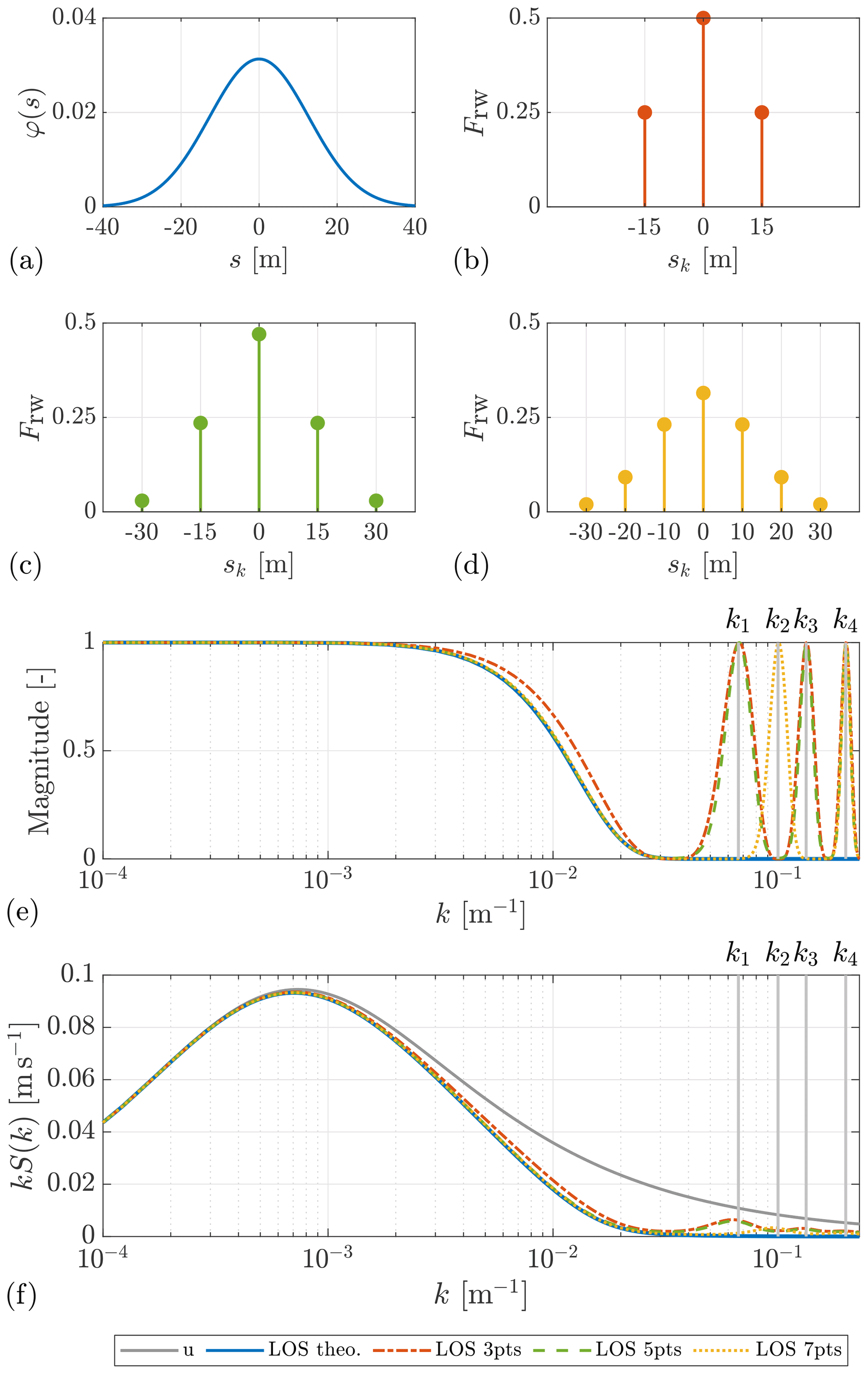
Figure 7 (a) Theoretical Gaussian-shape range weighting function with a full width at half maximum of 30 m for a pulsed lidar. (b–d) Three-point, five-point, and seven-point normalized discrete approximations of the range weighting function, with steps Δs_k of 15, 15, and 10 m, respectively. (e) Magnitudes of the FFTs of the different discretizations of the range weighting function. Critical wavenumbers: $k_{\mathrm{1}}=\mathrm{1}/\mathrm{15}{\mathrm{m}}^{-\mathrm{1}}$, $k_{\mathrm{2}}=\mathrm{1}/\mathrm{10}{\mathrm{m}}^{-\mathrm{1}}$, $k_{\mathrm{3}}=\mathrm{2}/\mathrm{15}{\mathrm{m}}^{-\mathrm{1}}$, and $k_{\mathrm{4}}=\mathrm{1}/\mathrm{5}{\mathrm{m}}^{-\mathrm{1}}$. (f) Theoretical auto-spectra of the u component and the LOS measurements of the different discretizations of the range weighting function. The LOS measurements are assumed aligned to the wind direction.

3.4 Impact of interpolation methods

In practice, the lidar simulation points are not necessarily located on the grid points of the simulated wind fields. To tackle this issue, one may consider using interpolation to approximate the values of the desired points for lidar simulations. In this section, we discuss the impact of interpolation on the auto-spectrum of the u component with two examples: nearest-neighbor interpolation and linear interpolation.

For simplicity, we consider a 2-by-2 square grid on the yz plane with a width of 5 m as shown in Fig. 8. The four vertices are defined as p₁(y₁,z₁), p₂(y₁,z₂), p₃(y₂,z₁), and p₄(y₂,z₂), for which the u components u_i (i=1 … 4) are simulated. The point to be interpolated is the center point of the square grid p₀(y₀,z₀).

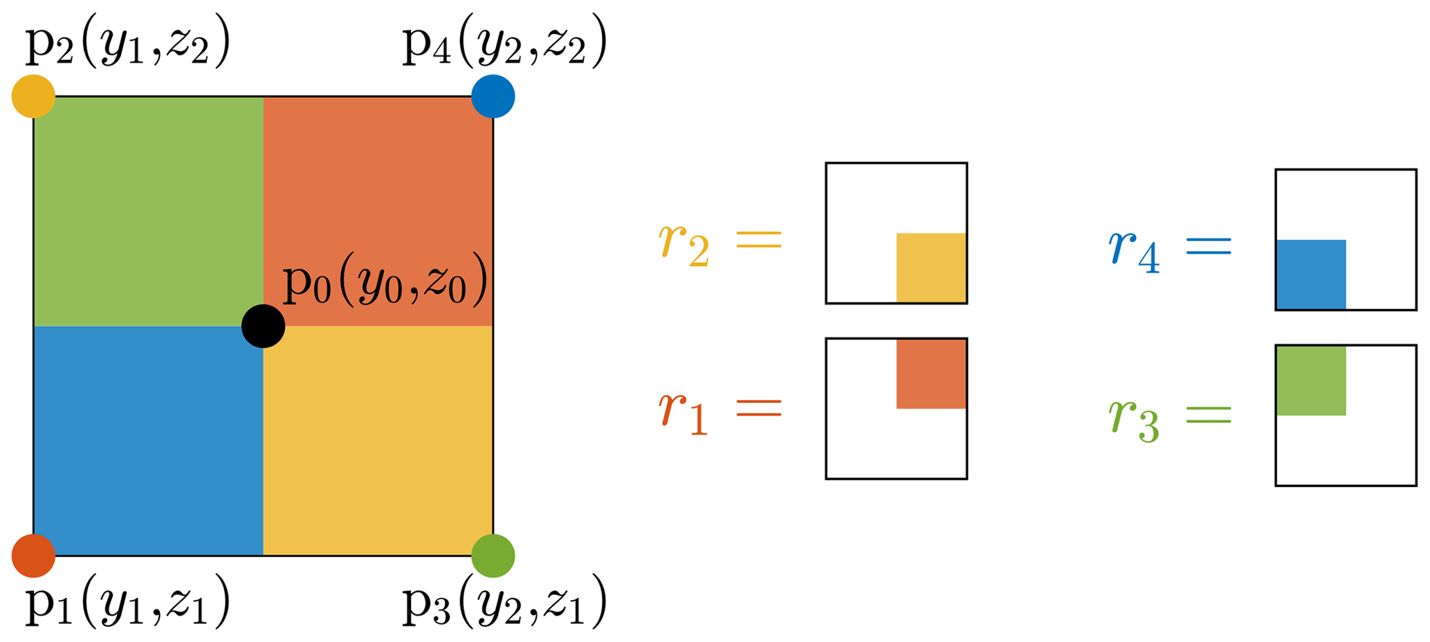
Figure 8 Visualization of 2D linear interpolation. The interpolated value at p₀ is calculated by the weighted mean of the values at neighboring grid points. The weighting factor r_i for the value at the point p_i is calculated according to the proportion of the partial area diagonally opposite the point p_i to the whole area, which is shown with corresponding colors.

Nearest-neighbor interpolation takes the value of the nearest point. In this example, u_0,nearest is approximated by u₁, and thus

$$\begin{array}{}\text{(42)}& S_{u_{\mathrm{0},\mathrm{nearest}}}=S_u.\end{array}$$

Apparently, using nearest-neighbor interpolation will not change the auto-spectrum.

Two-dimensional linear interpolation calculates u₀ by the weighted mean of the values neighboring grid points (Press et al., 2007):

$$\begin{array}{}\text{(43)}& u_{\mathrm{0},\mathrm{linear}}=\sum _{i=\mathrm{1}}^{\mathrm{4}}{r}_i{u}_i.\end{array}$$

The weighting factor r_i is calculated according to the proportion of the partial area diagonally opposite the point p_i to the whole area as illustrated in Fig. 8 with corresponding colors (Press et al., 2007):

$$\begin{array}{}\text{(44)}& \begin{array}{r}{r}_{\mathrm{1}}={\displaystyle \frac{(y_{\mathrm{2}}-y_{\mathrm{0}})(z_{\mathrm{2}}-z_{\mathrm{0}})}{(y_{\mathrm{2}}-y_{\mathrm{1}})(z_{\mathrm{2}}-z_{\mathrm{1}})}},r_{\mathrm{2}}={\displaystyle \frac{(y_{\mathrm{0}}-y_{\mathrm{1}})(z_{\mathrm{2}}-z_{\mathrm{0}})}{(y_{\mathrm{2}}-y_{\mathrm{1}})(z_{\mathrm{2}}-z_{\mathrm{1}})}},\\ r_{\mathrm{3}}={\displaystyle \frac{(y_{\mathrm{2}}-y_{\mathrm{0}})(z_{\mathrm{0}}-z_{\mathrm{1}})}{(y_{\mathrm{2}}-y_{\mathrm{1}})(z_{\mathrm{2}}-z_{\mathrm{1}})}},r_{\mathrm{4}}={\displaystyle \frac{(y_{\mathrm{0}}-y_{\mathrm{1}})(z_{\mathrm{0}}-z_{\mathrm{1}})}{(y_{\mathrm{2}}-y_{\mathrm{1}})(z_{\mathrm{2}}-z_{\mathrm{1}})}}.\end{array}\end{array}$$

The sum of the weighting factors equals one. Similar to Eq. (28), the auto-spectrum is computed by

$$\begin{array}{}\text{(45)}& \begin{array}{rl}{S}_{u_{\mathrm{0},\mathrm{linear}}}& =\mathcal{F}\left\{\sum _{i=\mathrm{1}}^{\mathrm{4}}{r}_i{u}_i\right\}{\mathcal{F}}^{*}\left\{\sum _{j=\mathrm{1}}^{\mathrm{4}}{r}_j{u}_j\right\}\\ & =\sum _{i=\mathrm{1}}^{\mathrm{4}}\sum _{j=\mathrm{1}}^{\mathrm{4}}{\mathit{\gamma }}_{u,yz,i,j}{r}_i{r}_j{S}_u,\end{array}\end{array}$$

with ${\mathit{\gamma }}_{u,yz,i,j}$ the coherence of the u component between the points i and j in the grid. Knowing the fact that

$$\begin{array}{}\text{(46)}& \begin{array}{rl}& {\mathit{\gamma }}_{u,yz,i,j}<\mathrm{1}\mathrm{and}{r}_i<\mathrm{1},\\ & S_{u_{\mathrm{0},\mathrm{linear}}}<S_u,\end{array}\end{array}$$

when the point to be interpolated does not overlap any existing grid points. Equation (45) means that using linear interpolation will decrease the auto-spectrum.

Figure 9 confirms that nearest-neighbor interpolation does not alter the auto-spectrum, while linear interpolation filters out the auto-spectrum especially in the high-frequency range because the coherence decays more for high frequencies. In fact, according to Eqs. (45) and (46), all interpolation methods based on weighted averaging of the values at neighboring grid points will reduce the auto-spectrum because the weighting factors must be multiplied with the coherence between the interpolated point and the corresponding neighboring points, which is always less than one. Consequently, we believe that nearest-neighbor interpolation is preferable in terms of maintaining the auto-spectrum.

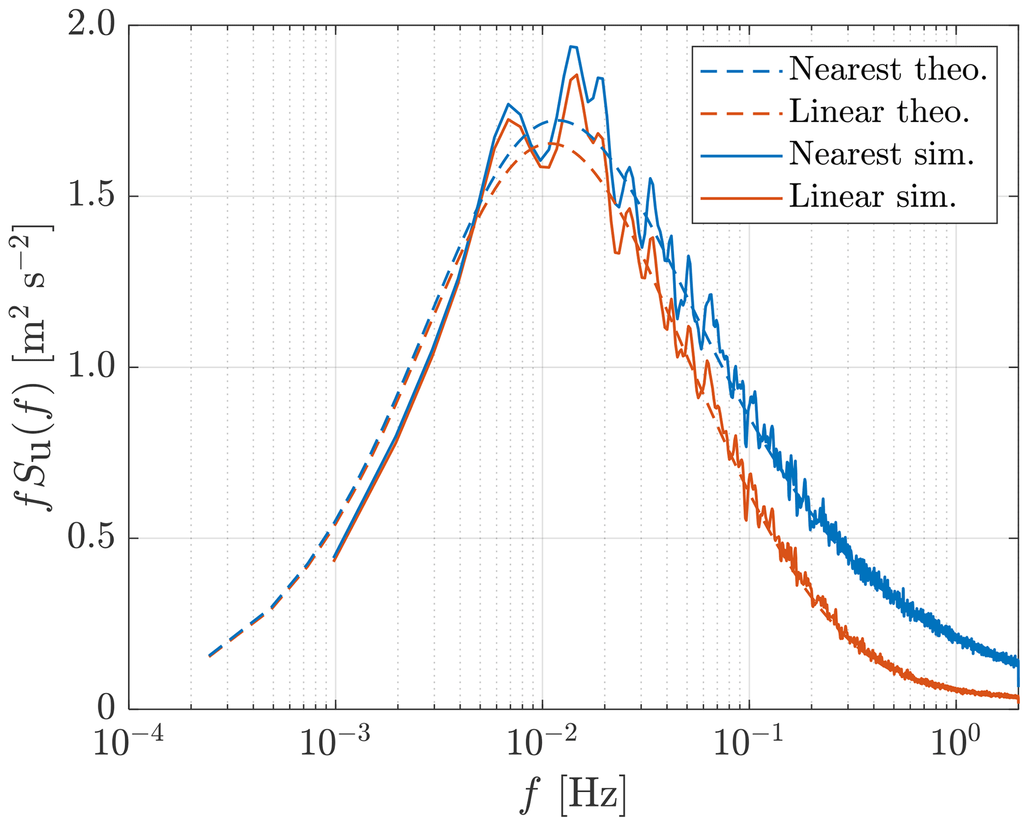
Figure 9 Comparison of the impact of nearest-neighbor interpolation and linear interpolation on the auto-spectrum of the u component. A 2-by-2 square grid on the yz plane with a width of 5 m is considered, and the point to be interpolated is the center point of the square grid. The auto-spectra are averaged with 16 samples.

3.5 Discussion about simulation grids

As discussed in Sect. 3.3, lidar simulations require a sufficiently dense grid of wind fields to avoid the effect of spatial discretization on the simulated auto-spectrum of LOS measurements. However, a dense grid makes 4D wind field generation computationally intensive according to its principle presented in Sect. 2. Given this situation, we attempt to propose an approximate method with a sparse grid – the “semi-frozen grid” – and compare it with two typical grids – the “direct grid” and the “full grid”. The definitions of these three types of simulation grids are introduced below.

If the position and the measuring trajectory of the lidar to be simulated are fixed, we can directly generate wind speeds at all the points required for lidar simulations, including the discrete points for modeling the volume averaging effect of lidars. We define this type of grid as the direct grid (see Fig. 10a). It is worth noting that because the direct grid is irregular, the method presented in Sect. 2.2 (see Eq. (8) should be applied to generate 4D wind fields. However, the direct grid is not applicable to simulations of a nacelle-mounted lidar because its position moves with the nacelle of a wind turbine in aeroelastic simulations. In this section, the direct grid actually serves as a reference for comparison because it does not require interpolation of wind speeds.

Figure 10 Illustration of three types of grids for lidar simulations. (a) Direct grid. (b) Full grid. (c) Semi-frozen grid.

To simulate a nacelle-mounted lidar, the grid of wind fields must cover all the range gates of the lidar and the space in their vicinity so that LOS measurements can be properly modeled when the required points constantly change due to the nacelle motion. For this purpose, we define the grid consisting of the vertical planes (perpendicular to x axis) with regular grid points at the x positions of the focus points and the discrete volumes of all range gates as the full grid (see Fig. 10b).

With the full grid method, the overall effects of both discrete ranging weighting functions (taking three-point and five-point cases as an example) and interpolation methods (linear or nearest) are illustrated in Fig. 11. The wind field is generated using the Kaimal model with the parameters listed in Table 1. The grid width on the y and z axes for the full grid is 5 m. A four-beam pulsed lidar with parameters listed in Table 2 is considered for the lidar simulations. The motion of lidar position is not taken into account in this comparison, and thus the lidar is assumed fixed at the coordinate system origin. Figure 11a shows that the auto-spectrum in high-frequency range of the three-point case slightly exceeds the theoretical curve when compared to the five-point case shown in Fig. 11b. Moreover, in both Fig. 11a and b, using linear interpolation slightly reduces the auto-spectrum in the range after the peak. As observed in Fig. 11c, both discrete ranging weighting functions and interpolation methods seem to have no influence on the coherence between the REWS and the lidar-estimated REWS.

Table 2 Parameters of the simulated pulsed lidar system.

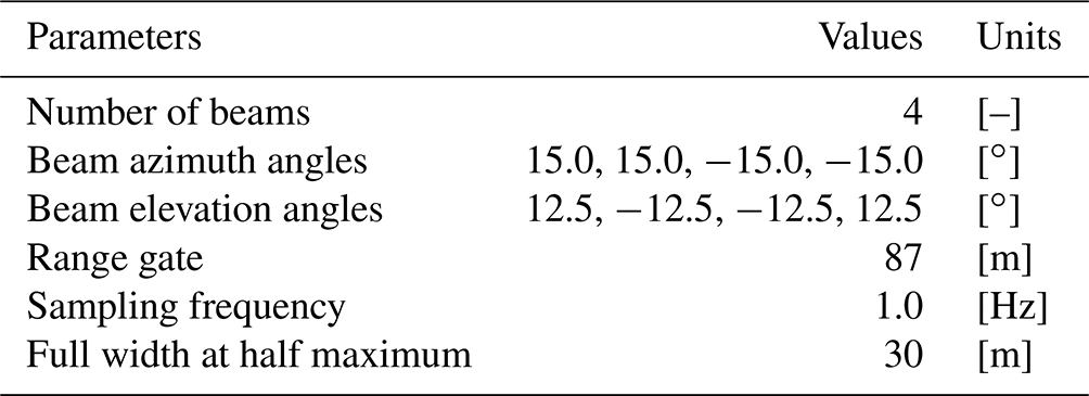
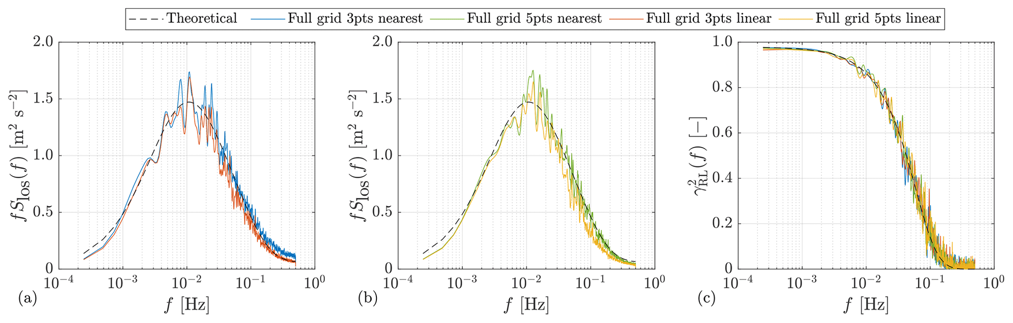
Figure 11 Comparison of the simulated lidar spectral properties with different discrete weighting functions and interpolation methods. (a, b) Auto-spectra of LOS measurements. (c) Coherence between rotor effective wind speed (REWS) and lidar-estimated REWS. The discrete weighting functions: three-point and five-point cases in accordance with Fig. 7. The interpolation methods: linear and nearest. The simulated auto-spectra are averaged with 16 samples.

However, using full grid for lidar simulations requires relatively high computational effort for the 4D wind field generation because it needs to generate the same number of 3D wind fields as the unique x positions required to simulate all discrete points of measurement gates. To reduce the computational effort of full grid, we propose an approximate method that combines 4D wind field generation and Taylor’s (1938) frozen hypothesis: a sparse grid which only contains the vertical planes with regular grid points at the x positions of the focus points of the lidar range gates is defined in the 4D wind field generation, and Taylor’s (1938) hypothesis is applied to the lidar probe volumes (which can be regarded as mini wind fields) to model the volume averaging effect. We define this method as the semi-frozen grid (see Fig. 10c). More specifically, Eq. (33) can be rewritten as

$$\begin{array}{}\text{(47)}& S_{u,i,j}={\mathit{\gamma }}_{\mathrm{s},i,j}{\mathit{\gamma }}_{x,i,j}{\mathit{\gamma }}_{yz,i,j}{S}_u\end{array}$$

following our previous assumptions in Sect. 2.3. The semi-frozen grid assumes frozen turbulence between i and j, i.e., the longitudinal coherence ${\mathit{\gamma }}_{x,i,j}=\mathrm{1}$ for any frequency.

To evaluate if the semi-frozen grid is a proper approximation, we compare these three grids by considering the auto-spectra of LOS measurements and the coherence between the REWS and the lidar-estimated REWS. Four-dimensional wind fields are generated in each of these three grids with the Kaimal model (for parameters, see Table 1). The grid width on the y and z axes for both the full grid and the semi-frozen grid is 5 m. For the lidar configuration, see Table 2. The motion of lidar position is not considered in this comparison. For simplicity, LOS measurements are simulated with three discrete points in the probe volumes. As shown in Fig. 12, the simulated auto-spectra and coherence in the three grids have no obvious difference, and they all match their theoretical curves given by the formulas derived in Sect. 3.2. Based on these results, we consider the semi-frozen grid to be a good compromise between the accuracy of lidar simulations and computational efforts of 4D wind field generation. However, because the simulation results depend on the properties of wind evolution and the lidar range weighting effect, the applicability of the semi-frozen grid to aeroelastic simulations of wind turbines should be verified according to specific conditions.

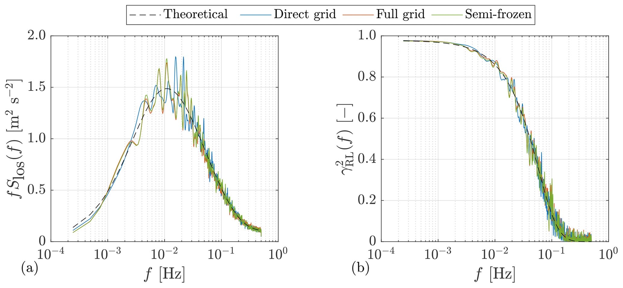
Figure 12 Comparison of the simulated lidar spectral properties with different grids. (a) Auto-spectra of LOS measurements. (b) Coherence between rotor effective wind speed (REWS) and lidar-estimated REWS. Direct grid: all the points required for lidar simulations are directly defined in the 4D wind field generation. Full grid: the vertical planes with regular grid points at the x positions of the focus points and the discrete volumes of the lidar range gates. Semi-frozen: the vertical planes with regular grid points at the x positions of the focus points of the lidar range gates. Beam azimuth angle: 15.0^∘. Beam elevation angle: 12.5^∘. Range gate: 87 m. The simulated auto-spectra are averaged with 16 samples.

4 Conclusions

Lidar-assisted control (LAC) of wind turbines is a control concept which takes advantage of a nacelle-mounted lidar (a remote sensing device) to measure upstream wind of a turbine to enable the turbine to preact to the incoming turbulence (see, e.g., Schlipf, 2015; Simley, 2015). The recent commercial certification of LAC has drawn more attention to this technology (Schlipf et al., 2018). Because LAC is a preview control strategy based on the upstream turbulence, an appropriate modeling of wind evolution is essential to evaluate the benefits of LAC for wind turbines in aeroelastic simulations. Therefore, the commonly used stochastic 3D wind field simulation methods (Veers, 1988; Mann, 1994), which do not consider wind evolution, are no longer sufficient for this propose.

Out of the need for a wind field generator capable of simulating wind evolution, in the first part of this paper, we present a general method for 4D (space–time) stochastic wind field generation based on the extension of the Veers method (Veers, 1988), which enables 4D wind field generation for arbitrary grids. To increase the applicability of the 4D method, we further propose a two-step Cholesky decomposition approach on the basis of the general method, which is applied to 4D wind field generation for regular grids under specific assumptions. The two-step Cholesky decomposition approach leads to the idea to generate a 4D wind field by combining multiple statistically independent 3D wind fields. Based on this concept, we have developed an open-access 4D wind field generator – evoTurb, which is coupled with TurbSim (specifically for the Kaimal model Kaimal et al., 1972) and Mann turbulence generator (MTG). This tool has two main advantages. (1) The modeling of wind evolution is introduced into the stochastic wind field generation without changing any other wind field properties generated by TurbSim or MTG, which is beneficial to integrating the 4D wind field generation with the current framework of the aeroelastic simulation of wind turbines. (2) Pre-generated 3D wind fields can be used to generate 4D wind fields, which significantly increases the computational efficiency of 4D wind field generation.

Because 4D wind field generation is supposed to be applied to simulations of LAC systems, in the second part of this paper, we study lidar simulations in 4D wind fields with respect to the following three aspects and provide corresponding suggestions.

1. Discrete lidar range weighting function. Because lidar simulations require a discrete lidar range weighting function, we analyze the impact of different spacing of the discrete range weighting function. It is found that the discretization will introduce an additional sinusoidal-shape coherence at the wavenumber of the reciprocal of the spacing into the auto-spectrum of the simulated lidar measurements but seems to have no influence on the coherence between the rotor effective wind speed (REWS) and the lidar-estimated REWS. Therefore, we suggest to choose the spacing of a discrete range weighting function according to the maximum relevant wavenumber in a specific application to prevent noise being introduced into the auto-spectrum in the relevant wavenumber range.

2. Interpolation methods. In practice, when the lidar simulation points are not exactly located on the grid points of the simulated wind fields, interpolation is used to approximate the values of the desired points for lidar simulations. Our analysis shows that nearest-neighbor interpolation does not affect the auto-spectrum, while interpolation methods based on weighted averaging of the values at neighboring grid points will filter out the auto-spectrum of the u component especially in the high-frequency range. The reason for the latter is that the weighting factors must be multiplied with the coherence between the neighboring points, which is always less than one. No obvious impact on the coherence between the REWS and the lidar-estimated REWS is observed for both interpolation methods. Consequently, we consider nearest-neighbor interpolation to be preferable in terms of maintaining the auto-spectrum.

3. Simulation grids. A sufficiently dense grid of wind fields is necessary for lidar simulations to avoid the negative effects of spatial discretization, but such a dense grid makes 4D wind field generation computationally expensive. This dilemma motivates us to propose an approximate method with a sparse grid – the semi-frozen grid. This method uses a sparse grid which only contains the vertical planes with regular grid points at the x positions of the focus points of the lidar range gates to generate 4D wind fields and applies Taylor’s (1938) hypothesis to the lidar probe volumes to model the volume averaging effect. It is confirmed that lidar simulations with the semi-frozen grid perform as well as the direct grid (the points required for lidar simulations are directly defined in the 4D wind field generation) and the full grid (the vertical planes with regular grid points at the x positions of the focus points and the discrete volumes of the lidar range gates). As a result, we believe that the semi-frozen grid is applicable to aeroelastic simulations of wind turbines under some conditions.

There is still space to improve evoTurb. For example, the impact of assuming the identical longitudinal coherence for the u and w components for the Mann model (Mann, 1994) should be examined. Moreover, the longitudinal coherence of the v component can be added to evoTurb if it is relevant for other applications. Regarding simulations of LAC systems, it is necessary to interface evoTurb with aeroelastic simulation environments of wind turbines, e.g., OpenFAST. In addition, it is well worthwhile to investigate the probability of different degrees of wind evolution occurring in nature to provide a better reference for defining the simulation requirements. Last but not least, long-term field testing is desired for the validation of LAC simulations with different wind evolution conditions in the future.

Appendix A: Turbulence models

In the stochastic wind field generation, the wind velocity fluctuations are assumed to be statistically stationary Gaussian processes or Gaussian fields, which can be completely characterized by their mean, variance, auto-spectrum, and cross-spectra between any two spatial points (Pope, 2000). As evoTurb is made compatible with the TurbSim and Mann turbulence generator (MTG), the turbulence models deployed in both tools are briefly introduced in this section. For more details, please refer to ().

Before giving the formulas of both turbulence models, a general definition of the spatial coherence between the wind components i and j ($i,j=u,v,w$) at two spatially separated locations k and l is given as follows:

$$\begin{array}{}\text{(A1)}& {\mathit{\gamma }}_{ij,k,l}\left(f\right)={\displaystyle \frac{\left|S_{ij,k,l}\right(f\left)\right|}{\sqrt{S_{i,k}\left(f\right)S_{j,l}\left(f\right)}}},\end{array}$$

with f the frequency in hertz (Hz), S_i,k(f) and S_j,l(f) the respective auto-spectra, and $S_{ij,k,l}\left(f\right)$ the cross-spectrum.

The Kaimal spectral and exponential coherence model (Kaimal et al., 1972) is the most commonly used turbulence model in TurbSim. The non-dimensional auto-spectrum for the wind component i ($i=u,v,w$) is a function of the integral scale parameter L_i and wind speed at hub height V_hub:

$$\begin{array}{}\text{(A2)}& {\displaystyle \frac{f{S}_i\left(f\right)}{{\mathit{\sigma }}_i^{\mathrm{2}}}}={\displaystyle \frac{\mathrm{4}\cdot \frac{f{L}_i}{V_{\mathrm{hub}}}}{{\left(\mathrm{1}+\mathrm{6}\cdot \frac{f{L}_i}{V_{\mathrm{hub}}}\right)}^{\mathrm{5}/\mathrm{3}}}},\end{array}$$

with S_i the one-sided auto-spectrum and σ_i the standard deviation of the corresponding wind speed component.

In this model, only the spatial coherence for the u component on the same yz plane (indicated with the subscript “yz”) is considered using an exponential coherence model:

$$\begin{array}{}\text{(A3)}& {\mathit{\gamma }}_{u,yz}(d_{yz},f)=\exp \left[-\mathrm{12}\sqrt{{\left({\displaystyle \frac{f{d}_{yz}}{V_{\mathrm{hub}}}}\right)}^{\mathrm{2}}+{\left(\mathrm{0.12}\cdot {\displaystyle \frac{d_{yz}}{L_u}}\right)}^{\mathrm{2}}}\right],\end{array}$$

where d_yz is an entry of a matrix containing separations between any pair of points on the yz plane.

The Mann uniform (Mann, 1994) shear turbulence model is the model deployed in the MTG. The two-sided 1D (the x direction) spectra of Mann model can be computed with

$$\begin{array}{}\text{(A4)}& F_{ij}\left(k_{\mathrm{1}}\right)=\underset{-\mathrm{\infty }}{\overset{\mathrm{\infty }}{\int }}\underset{-\mathrm{\infty }}{\overset{\mathrm{\infty }}{\int }}{\mathrm{\Phi }}_{ij}(k_{\mathrm{1}},k_{\mathrm{2}},k_{\mathrm{3}})\mathrm{d}{k}_{\mathrm{2}}\mathrm{d}{k}_{\mathrm{3}},\end{array}$$

where Φ_ij is the spectral tensor defining the ensemble mean of the Fourier coefficient of the wind components ($i,j=\mathrm{1},\mathrm{2}$, or 3 stands for $u,v,w$) (see, e.g., Peña et al., 2017; Held and Mann, 2019). k₁, k₂, and k₃ are the spatial wavenumbers for the three wind component directions. For brevity, the spectral tensor ${\mathrm{\Phi }}_{ij}(k_{\mathrm{1}},k_{\mathrm{2}},k_{\mathrm{3}})$ is not explicitly given in this paper. Please refer to Mann (1994) or () for more details.

The magnitude coherence (no square) for spatial separations perpendicular to the longitudinal direction can be obtained by

$$\begin{array}{}\text{(A5)}& \begin{array}{rl}& {\mathit{\gamma }}_{ij,yz}(k_{\mathrm{1}},\mathrm{\Delta }y,\mathrm{\Delta }z)\\ & ={\displaystyle \frac{\left|{\int }_{-\mathrm{\infty }}^{\mathrm{\infty }}{\int }_{-\mathrm{\infty }}^{\mathrm{\infty }}{\mathrm{\Phi }}_{ij}(k_{\mathrm{1}},k_{\mathrm{2}},k_{\mathrm{3}}){\mathrm{e}}^{-\mathbf{\text{i}}{k}_{\mathrm{2}}\mathrm{\Delta }y}{\mathrm{e}}^{-\mathbf{\text{i}}{k}_{\mathrm{3}}\mathrm{\Delta }z}\mathrm{d}{k}_{\mathrm{2}}\mathrm{d}{k}_{\mathrm{3}}\right|}{\sqrt{F_{ii}\left(k_{\mathrm{1}}\right)F_{jj}\left(k_{\mathrm{1}}\right)}}},\end{array}\end{array}$$

where Δy and Δz are spatial separations for lateral and vertical directions, and i is the imaginary unit. The frequency spectra or coherence of the Mann model can be obtained using the conversion $k_{\mathrm{1}}=\mathrm{2}\mathit{\pi }f/V_{\mathrm{hub}}$ with the help of Taylor's frozen hypothesis (Mann, 1998).

Appendix B: Wind evolution models

Simley and Pao (2015)Chen et al. (2021)Kristensen (1979)

Table B1 Summary of the wind evolution models supported in evoTurb. d_x is the spatial separation on the wind direction. $\stackrel{\mathrm{‾}}{U}$ is the mean wind speed. σ is related to the total turbulent kinetic energy and can be calculated through $\sqrt{{\mathit{\sigma }}_u^{\mathrm{2}}+{\mathit{\sigma }}_v^{\mathrm{2}}+{\mathit{\sigma }}_w^{\mathrm{2}}}$. L_u is the integral length scale of the u component. 𝒢𝒫ℛ(⋅) denotes a Gaussian process regression model. For brevity, the predictors (i.e., input variables) are not explicitly listed in the table. For more details, please refer to the open-access tool evoTurb.

Wind evolution refers to the decorrelation of turbulence structures (eddies) dependent on evolution time. Following previous research (see, e.g., Pielke and Panofsky, 1970; Kristensen, 1979; Simley and Pao, 2015; Schlipf et al., 2015; Chen et al., 2021), wind evolution is measured by the longitudinal coherence between velocity fluctuations at different locations in the longitudinal direction. Its definition is analogous to the lateral–vertical coherence, but it corresponds to a lagged correlation, which means when calculating the longitudinal coherence, one of the wind speeds should be shifted by the corresponding time lag between both wind speeds.

Currently, only the longitudinal coherence of the u component γ_u,x is considered. To model γ_u,x, evoTurb supports different wind evolution models proposed in some previous studies (see Table B1). It is worth mentioning that these models are provided in the form of the magnitude-squared coherence ${\mathit{\gamma }}_{u,x}^{\mathrm{2}}$ in the literature, and thus the square root needs to be taken when applied to the 4D wind field generation. The models can be categorized as empirical and physical. The first two models are empirical models following a similar simple exponential form. They are all based on the same assumption that turbulent eddies decay exponentially but consider different model parameters (Simley and Pao, 2015; Chen et al., 2021). The last model is a physical deduced model which assumes that the coherence can be modeled with the square of the probability that an eddy observed at the first location can also be observed at the second location. This considers two probabilities: the probability that the eddy does not decay during its travel, which is also modeled with the exponential expression, and the probability that the eddy is carried towards the second location, which is modeled with the transversal diffusion of eddies (Kristensen, 1979). For more details regarding these wind evolution models, please refer to the corresponding references.

Appendix C: Mathematical proof for the Cholesky decomposition of the Kronecker product

The Kronecker product (Henderson et al., 1983) is a special multiplication operation on two matrices of arbitrary size, which gives a block matrix as a result. For an m-by-n matrix P and a p-by-q matrix Q, the Kronecker product P⊗Q is a pm-by-qn block matrix defined as

$$\begin{array}{}\text{(C1)}& \mathbf{P}\otimes \mathbf{Q}=\left[\begin{array}{ccc}{p}_{\mathrm{1},\mathrm{1}}\mathbf{Q}& \mathrm{\dots }& p_{\mathrm{1},n}\mathbf{Q}\\ \mathrm{⋮}& \mathrm{\ddots }& \mathrm{⋮}\\ p_{m,\mathrm{1}}\mathbf{Q}& \mathrm{\dots }& p_{m,n}\mathbf{Q}\end{array}\right].\end{array}$$

According to Schacke (2004), the Kronecker product has the following properties for the real matrices P, Q, M, and N:

$$\begin{array}{}\text{(C2)}& {\displaystyle }(\mathbf{\text{P}}\otimes \mathbf{Q}{)}^{\top }={\mathbf{P}}^{\top }\otimes {\mathbf{Q}}^{\top };\text{(C3)}& {\displaystyle }(\mathbf{P}\otimes \mathbf{Q})(\mathbf{M}\otimes \mathbf{N})=\left(\mathbf{PM}\right)\otimes \left(\mathbf{QN}\right).\end{array}$$

The Cholesky decomposition (Press et al., 2007) can decompose a real, symmetric, positive-definite matrix A into the product of a lower triangular matrix L_A, i.e., the Cholesky factor, and its transpose:

$$\begin{array}{}\text{(C4)}& \mathbf{A}={\mathbf{L}}_{\mathbf{A}}{\mathbf{L}}_{\mathbf{A}}^{\top }.\end{array}$$

The operation to obtain the Cholesky factor is defined as

$$\begin{array}{}\text{(C5)}& {\mathbf{L}}_{\mathbf{A}}=\text{chol}\left(\mathbf{A}\right).\end{array}$$

With the above-mentioned properties, we can extend the Kronecker product of two real, symmetric, positive-definite matrices A and B as

$$\begin{array}{}\text{(C6)}& \begin{array}{rl}\mathbf{A}\otimes \mathbf{B}& =\left({\mathbf{L}}_{\mathbf{A}}{\mathbf{L}}_{\mathbf{A}}^{\top }\right)\otimes \left({\mathbf{L}}_{\mathbf{B}}{\mathbf{L}}_{\mathbf{B}}^{\top }\right)\\ & =({\mathbf{L}}_{\mathbf{A}}\otimes {\mathbf{L}}_{\mathbf{B}})({\mathbf{L}}_{\mathbf{A}}^{\top }\otimes {\mathbf{L}}_{\mathbf{B}}^{\top })\\ & =({\mathbf{L}}_{\mathbf{A}}\otimes {\mathbf{L}}_{\mathbf{B}})({\mathbf{L}}_{\mathbf{A}}\otimes {\mathbf{L}}_{\mathbf{B}}{)}^{\top }\end{array},\end{array}$$

with L_A and L_B the Cholesky factors of A and B, respectively. By applying the Cholesky decomposition to Eq. (C6), we can prove that

$$\begin{array}{}\text{(C7)}& \begin{array}{rl}\text{chol}(\mathbf{A}\otimes \mathbf{B})& =\text{chol}\left(\right({\mathbf{L}}_{\mathbf{A}}\otimes {\mathbf{L}}_{\mathbf{B}}\left)\right({\mathbf{L}}_{\mathbf{A}}\otimes {\mathbf{L}}_{\mathbf{B}}{)}^{\top })\\ & ={\mathbf{L}}_{\mathbf{A}}\otimes {\mathbf{L}}_{\mathbf{B}}\\ & =\text{chol}\left(\mathbf{A}\right)\otimes \text{chol}\left(\mathbf{B}\right).\end{array}\end{array}$$