Wake properties and power output of very large wind farms for different meteorological conditions and turbine spacings: a large-eddy simulation case study for the German Bight

Germany's expansion target for offshore wind power capacity of 40 GW by the year 2040 can only be reached if large portions of the Exclusive Economic Zone in the German Bight are equipped with wind farms. Because these wind farm clusters will be much larger than existing wind farms, it is unknown how they will affect the boundary layer flow and how much power they will produce. The objective of this large-eddy simulation study is to investigate the wake properties and the power output of very large potential wind farms in the German Bight for different turbine spacings, stabilities and boundary layer heights. The results show that very large wind farms cause flow effects that small wind farms do not. These effects include, but are not limited to, inversion layer displacement, counterclockwise flow deflection inside the boundary layer and clockwise flow deflection above the boundary layer. Wakes of very large wind farms are longer for shallower boundary layers and smaller turbine spacings, reaching values of more than 100 km. The wake in terms of turbulence intensity is approximately 20 km long, in which longer wakes occur for convective boundary layers and shorter wakes for stable boundary layers. Very large wind farms in a shallow, stable boundary layer can excite gravity waves in the overlying free atmosphere, resulting in significant flow blockage. The power output of very large wind farms is higher for thicker boundary layers because thick boundary layers contain more kinetic energy than thin boundary layers. The power density of the energy input by the geostrophic pressure gradient limits the power output of very large wind farms. Because this power density is very low (approximately 2 W m⁻²), the installed power density of very large wind farms should be small to achieve a good wind farm efficiency.

1 Introduction

At present, the global installed wind power capacity from offshore wind farms is increasing rapidly. According to the expansion targets of the current leading offshore wind markets (the United Kingdom, Germany and China), the offshore wind power capacity will be subject to significant growth over the next decades. The German expansion target for offshore wind power capacity is 40 GW by the year 2040, which is more than the global installed offshore wind power capacity of 32.5 GW in the year 2020 (WindSeeG, 2020; Herzig, 2020). The otherwise undisturbed flow at offshore sites will be increasingly modified by wind farms, affecting the wind farm power output but also the meteorological conditions in the wake. For wind farms with a state-of-the-art size of approximately 100 turbines and a length of approximately 5 km, these effects have been extensively investigated experimentally and numerically and are generally well understood.

However, the size of future wind farms or clusters of wind farms will be 1 or 2 orders of magnitude larger than today's (see Fig. 1). Because no wind farms of this size exist currently, new insights into the behavior of the flow through wind farms and the resulting power output can only be provided by simulations. The most accurate method that resolves all the relevant processes such as the turbulent momentum and heat transport that is still computationally feasible is large-eddy simulation. In recent years many large-eddy simulations of wind farm flows have been carried out. A comprehensive review can be found in Porté-Agel et al. (2020). Some of the investigations consisted of an infinite wind farm setup with cyclic boundary conditions in the streamwise and crosswise directions (e.g., Lu and Porté-Agel, 2011; Calaf et al., 2011; Johnstone and Coleman, 2012). With these methods, the limiting case of an infinite wind farm can be investigated at relatively low computational cost due to the small domain size. Johnstone and Coleman (2012) used this method to compare a neutral boundary layer flow with and without wind turbines. The wind turbines increased the boundary layer height and the ageostrophic wind component inside the boundary layer, which led to a higher energy input by the pressure gradient. Simple one-dimensional models for the wind speed profile inside and above an infinite wind farm have been developed by, for example, Frandsen (1992), Calaf et al. (2010), and Abkar and Porté-Agel (2013).

Some authors used a semi-infinite wind farm setup with cyclic boundary conditions only in the crosswise direction (Stevens et al., 2016; Allaerts and Meyers, 2017; Wu and Porté-Agel, 2017). Allaerts and Meyers (2017) simulated a 15 km long wind farm in a conventionally neutral boundary layer (CNBL) with different heights. In the shallow boundary layer cases, the wind-farm-induced flow deceleration led to upward displacement of the inversion layer which triggered stationary gravity waves in the free atmosphere. These gravity waves can impose favorable and unfavorable streamwise pressure gradients upstream, inside and downstream of the wind farm, which can result in significant flow acceleration or deceleration.

Large-eddy simulations of existing wind farms have been carried out, e.g., the wind farms Horns Rev with eighty 2 MW turbines (Porté-Agel et al., 2013; Wu and Porté-Agel, 2015), Alpha Ventus with twelve 5 MW turbines, Lillgrund with 48 2.3 MW turbines (Churchfield et al., 2012; Nilsson et al., 2015) and EnBW Baltic 1 with twenty-one 2.3 MW turbines (Witha et al., 2014).

To date, there have been no studies of wind farms of finite size with variable meteorological conditions, nor have spatial and energy scales of future wind farms (on the order of 100 km and 10 GW) been investigated. With this study we want to fill this gap by performing large-eddy simulations of very large, finite size wind farms for different stabilities, turbine spacings and boundary layer heights. We provide new insights into the wake properties and power output of very large wind farms and how these depend on the varied parameters. Specifically we want to answer these questions.

1. How is the flow inside and above the boundary layer affected by very large wind farms?

2. How long is the wake in terms of speed deficit and turbulence intensity?

3. What physical processes drive the wake recovery?

4. How much power output or power density can be expected for very large wind farms?

5. What effect does the turbine spacing and the boundary layer height have on questions 1–4?

Instead of using an idealized wind farm shape, we investigate a potential future wind farm scenario in the German Bight, which is shown in Fig. 1. The scenario assumes that all priority areas for future wind farms are equipped with 15 MW wind turbines. This results in a total number of up to 2088 wind turbines with a total wind farm capacity of up to 31 GW. More than 7 billion grid points are required to fill the large domain with a turbine wake-resolving grid. The simulations were carried out on 5120 cores on one of the supercomputers of the North German Supercomputing Alliance (HLRN). A simulation required a wall-clock time of 25 to 50 h. To our knowledge, this large-eddy simulation case study exceeds other studies in terms of wind farm area and total wind turbine number by at least 1 order of magnitude.

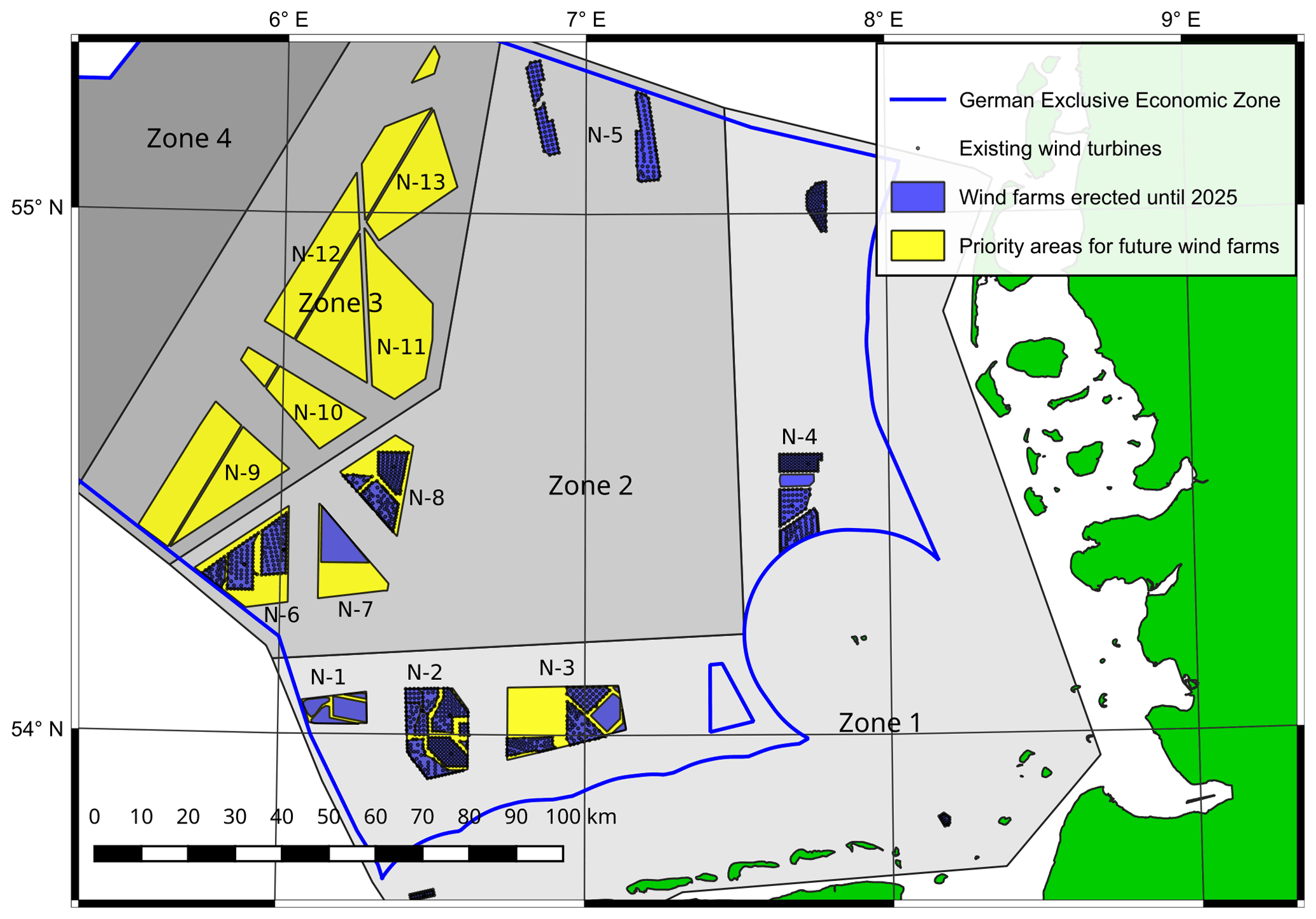
Figure 1 Existing wind farms and priority areas for future wind farms in the German Exclusive Economic Zone in the German Bight. The map is based on data that are publicly available at https://www.geoseaportal.de (last access: 4 March 2021).

The numerical model, setup and boundary conditions are described in Sect. 2. The simulation results regarding the wake properties and the power output are shown and discussed in Sect. 3. Section 4 concludes and discusses the results of the study.

2 Methods

2.1 Numerical model

The simulations were performed with the Parallelized Large-eddy Simulation Model (PALM) (Maronga et al., 2020), which is developed at the Institute of Meteorology and Climatology of Leibniz Universität Hannover, Germany. Several wind farm flow investigations have been successfully conducted with this code in the past (e.g., Witha et al., 2014; Dörenkämper et al., 2015). PALM solves the non-hydrostatic, incompressible Navier–Stokes equations in Boussinesq-approximated form. The equations for the conservation of mass, momentum and internal energy spatially filtered over a grid volume then read as follows:

$$\begin{array}{}\text{(1)}& {\displaystyle \frac{\partial u_j}{\partial x_j}}=\mathrm{0},\end{array}$$

$$\begin{array}{}\text{(2)}& \begin{array}{rl}{\displaystyle \frac{\partial u_i}{\partial t}}& =-{\displaystyle \frac{\partial u_i{u}_j}{\partial x_j}}-{\mathit{ϵ}}_{ijk}{f}_j{u}_k+{\mathit{ϵ}}_{i\mathrm{3}j}{f}_{\mathrm{3}}{u}_{g,j}\\ & -{\displaystyle \frac{\mathrm{1}}{{\mathit{\rho }}_{\mathrm{0}}}}{\displaystyle \frac{\partial {\mathit{\pi }}^{\ast }}{\partial x_i}}+g{\displaystyle \frac{\mathit{\theta }-\langle \mathit{\theta }\rangle }{\langle \mathit{\theta }\rangle }}{\mathit{\delta }}_{i\mathrm{3}}-{\displaystyle \frac{\partial }{\partial x_j}}(\stackrel{\mathrm{‾}}{u_i^{\prime \prime }{u}_j^{\prime \prime }}-{\displaystyle \frac{\mathrm{2}}{\mathrm{3}}}e{\mathit{\delta }}_{ij}),\end{array}\end{array}$$

$$\begin{array}{}\text{(3)}& {\displaystyle \frac{\partial \mathit{\theta }}{\partial t}}=-{\displaystyle \frac{\partial u_j\mathit{\theta }}{\partial x_j}}-{\displaystyle \frac{\partial }{\partial x_j}}\left(\stackrel{\mathrm{‾}}{u_i^{\prime \prime }{\mathit{\theta }}^{\prime \prime }}\right),\end{array}$$

where angular brackets indicate horizontal averaging, and a double prime indicates subgrid-scale (SGS) quantities, $i,j,k\in \mathit{\{}\mathrm{1},\mathrm{2},\mathrm{3}\mathit{\}}$, u_i, u_j, u_k are the velocity components in the respective directions (x_i, x_j, x_k), θ is potential temperature, t is time, $f_i=(\mathrm{0},\mathrm{2}\mathrm{\Omega }\cos (\mathit{\varphi })$, 2Ωsin (ϕ)) is the Coriolis parameter with the Earth's angular velocity $\mathrm{\Omega }=\mathrm{0.729}\times {\mathrm{10}}^{-\mathrm{4}}\mathrm{rad}{\mathrm{s}}^{-\mathrm{1}}$ and the geographical latitude ϕ. The geostrophic wind speed components are u_g,j, and the basic state density of dry air is ρ₀. The modified perturbation pressure is ${\mathit{\pi }}^{\ast }=p^{\ast }+\frac{\mathrm{2}}{\mathrm{3}}{\mathit{\rho }}_{\mathrm{0}}e$, where p^∗ is the perturbation pressure, and $e=\frac{\mathrm{1}}{\mathrm{2}}\stackrel{\mathrm{‾}}{u_i^{\prime \prime }{u}_i^{\prime \prime }}$ is the SGS turbulence kinetic energy. The gravitational acceleration is $g=\mathrm{9.81}\mathrm{m}{\mathrm{s}}^{-\mathrm{2}}$, and δ is the Kronecker delta.

The SGS model uses a 1.5-order closure according to Deardorff (1980), modified by Moeng and Wyngaard (1988) and Saiki et al. (2000). Recently, the modified version of Dai et al. (2021) has been implemented in PALM, which allows for coarser grid spacings in stable boundary layers due to reduced grid spacing sensitivity. This modified version is used for the simulation of wind farms in a stable boundary layer.

The following features of PALM are relevant for the performed simulations. It is possible to prescribe a surface heating or cooling rate instead of prescribing a surface heat flux. Stable boundary layers can also be generated by imitating warm air advection by using a large-scale forcing. Convective boundary layer growth can be compensated for by applying a large-scale subsidence to the potential temperature field. A Rayleigh damping layer can be used in order to avoid gravity wave reflection at the top of the domain.

The wind turbines are represented by an advanced actuator disc model with rotation (ADM-R) that acts as an axial momentum sink and an angular momentum source (inducing wake rotation). The ADM-R is described in detail by Steinfeld et al. (2015) and Wu and Porté-Agel (2011). The actuator disc is divided into several segments along the radial and tangential directions to allow for a non-uniform thrust distribution over the disc. The lift and thrust force of each segment f_l and f_d is projected on the axial (f_a) and tangential (f_t) directions:

$$\begin{array}{}\text{(4)}& f_{\mathrm{a}}=-f_{\mathrm{l}}\cos \mathrm{\Phi }-f_d\sin \mathrm{\Phi },f_{\mathrm{t}}=-f_{\mathrm{l}}\sin \mathrm{\Phi }-f_d\cos \mathrm{\Phi },\end{array}$$

where Φ is the angle between the local wind vector and the disc. The rotor thrust F and torque M are then calculated as the sum over all N segments at radius r_i:

$$\begin{array}{}\text{(5)}& F=\sum _{i=\mathrm{1}}^N{f}_{\mathrm{a},i},M=\sum _{i=\mathrm{1}}^N{f}_{\mathrm{t},i}{r}_i.\end{array}$$

The wind turbine power is calculated out of the rotational speed of the rotor n_rotor and the torque:

$$\begin{array}{}\text{(6)}& P=\mathrm{2}\mathit{\pi }{n}_{\mathrm{rotor}}M.\end{array}$$

To avoid numerical instabilities, the disc element forces are distributed to the neighboring grid points by a three-dimensional Gaussian smearing kernel, which is approximated by a computationally less expensive fourth-order polynomial. The smearing kernel has a default radius of 2Δx, reaching approximately 78 grid points. The otherwise two-dimensional actuator disc is enlarged in the axial and radial directions by the smearing, resulting in a power overestimation of 26.8 %. The power overestimation can be reduced to 12.5 % by setting the kernel radius to 1Δx, reaching approximately 10 grid points, without any numerical instabilities. The thrust coefficient is overestimated by 2 % for 2Δx and underestimated by 4 % for 1Δx. As a compromise, the smearing kernel radius is set to 1Δx for this study. The wind turbine power output is corrected for the power overestimation by a factor of $\mathrm{1}/\mathrm{1.125}$ before entering the wind farm power output analysis.

2.2 Case selection

To produce meaningful and relevant results, the simulations should represent the most common meteorological conditions in the German Bight. A climatology with frequency distributions of wind speed, wind direction, boundary layer (BL) height and stability information extracted from the COSMO-REA6 reanalysis dataset can be found in Appendix A. The analysis was provided by Thomas Spangehl (German Weather Service), and it is based on hourly data of a 24-year period (1995–2018) at 54^∘30^′ N, 6^∘00^′ E, which is located inside Zone 3 (see Fig. 1). Wind speed and direction are evaluated at 178 m height, which is the closest COSMO model level to the hub height of 150 m of the wind turbine used in the simulations.

Due to the high computational cost per simulation, only a limited number of simulations were carried out. This study consists of five simulations with varying stability, turbine spacing and BL height. An overview is given in Table 1. Two cases with a neutral boundary layer (NBL), two cases with a convective boundary layer (CBL) and one case with a stable boundary layer (SBL) are simulated.

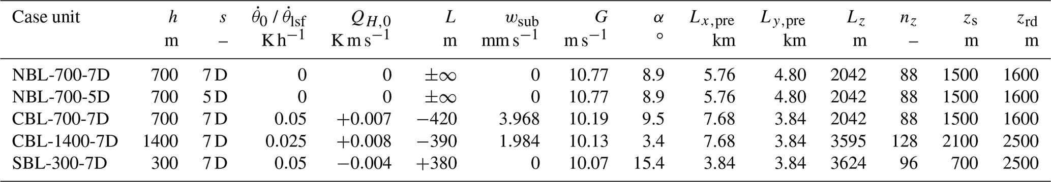
Table 1 Overview of simulated cases with boundary layer height h, turbine spacing s, surface heating rate ${\dot{\mathit{\theta }}}_{\mathrm{0}}$ or large-scale forcing advection tendency ${\dot{\mathit{\theta }}}_{\mathrm{lsf}}$ in the case of SBL-300-7D, surface heat flux Q_H,0, Monin–Obukhov length L, subsidence velocity w_sub, geostrophic wind speed G and direction α, length and width of the precursor domain L_x,pre and L_y,pre, domain height L_z, number of vertical grid points n_z, stretch level z_s, and Rayleigh damping level z_rd.

In the two NBL cases, NBL-700-5D and NBL-700-7D, the turbine spacing is set to s=5 D and s=7 D, where D is the rotor diameter of the turbine. The turbine spacing for all other cases is s=7 D. The NBL is capped by an inversion layer with a lapse rate of $\mathrm{\Gamma }=+\mathrm{1}$ K km⁻¹ to achieve a BL height of approximately 700 m, which is a very common BL height in the German Bight, according to the COSMO-REA6 climatology (see Figs. A3 and A4). The correct term for such an inversion-capped NBL is conventionally neutral boundary layer (CNBL). However, the cases are named NBL-700-7D and NBL-700-5D to avoid confusion with the CBL cases.

Because CBLs are more frequent and are generally thicker than SBLs in the German Bight, two CBL cases, CBL-700-7D and CBL-1400-7D, with a BL height of h≈700 and h≈1400 m, respectively, are simulated. This represents the spread of CBL heights in the German Bight (see Fig. A3). Note that a CBL is the only BL type for which the BL height can be controlled freely by the initial temperature profile without the need to change other parameters. The (steady-state) BL height of CNBLs and SBLs can not be controlled directly but is rather a function of friction velocity, Coriolis parameter, free atmosphere (FA) stratification and surface buoyancy flux (Zilitinkevich et al., 2007).

The BL height of the SBL case SBL-300-7D is h≈300 m so that the wind turbines with a rotor top height of 270 m are still within the BL and do not penetrate into the FA; 300 m is a small but still typical value for an SBL in the German Bight (see Fig. A4).

The wind speed at hub height is set to 10 m s⁻¹ for all cases. This wind speed is less than the mean wind speed in the German Bight (10.8 m s⁻¹, see Fig. A1) to stay below the rated wind speed of $v_{\mathrm{rated}}=\mathrm{10.59}\mathrm{m}{\mathrm{s}}^{-\mathrm{1}}$ of the IEA 15 MW reference wind turbine (Gaertner et al., 2020). Thus the turbine operates at a high thrust coefficient, and the turbine power is a function of the wind speed. The surface roughness length in all cases is z₀=1 mm. The wind direction at hub height is set to 225^∘ by tuning the geostrophic wind direction α appropriately (see Table 1). Southwest wind is one of the most common wind directions in the German Bight. Because the main axis of the wind farm clusters in Zone 3 has a southwest–northeast orientation, strong wake effects can be expected for this wind direction.

2.3 Setup, boundary conditions, domain and wind farm layout

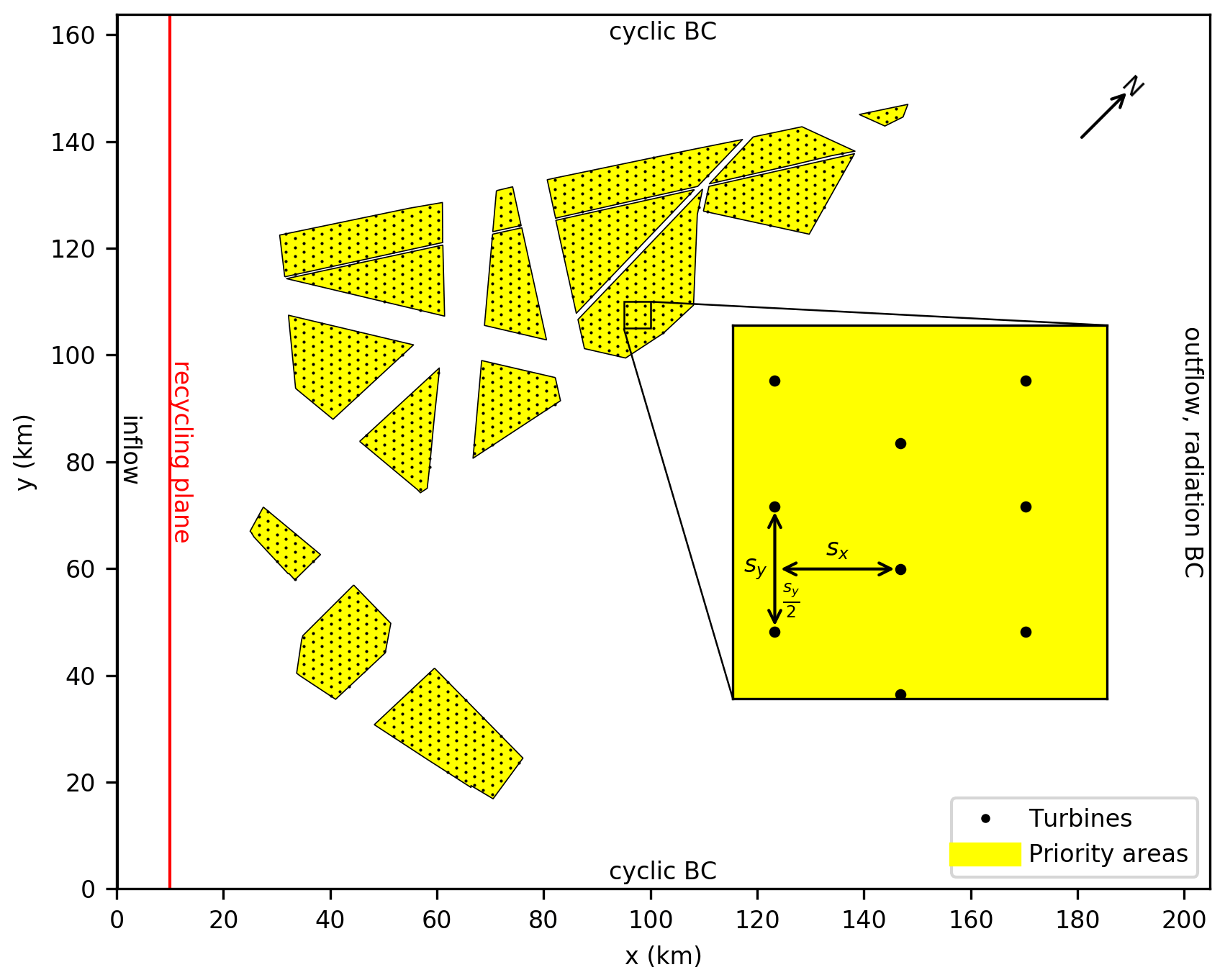
Figure 2 Domain and wind farm layout: inflow from left and turbulence recycling plane at x=10 km. Priority areas for future wind farms (see Fig. 1) are filled with a regular, staggered grid of wind turbines with a streamwise and crosswise turbine spacing of $s_x=s_y=\mathrm{7}$ D (shown here) or 5 D.

The domain and wind farm layout are shown in Fig. 2. The domain length and width are L_x=204.8 km and L_y=163.84 km, respectively. These lengths correspond to n_x=10 240 and n_y=8192 grid points in the x and y directions for isotropic grid spacings of $\mathrm{\Delta }x=\mathrm{\Delta }y=\mathrm{\Delta }z=\mathrm{20}$ m for all cases. These spacings yield a density of 12 grid points per rotor diameter, which is enough to resolve the most relevant eddies inside the wind turbine wakes. As Steinfeld et al. (2015) showed, even eight grid points per rotor diameter are sufficient to obtain a converged result for the mean wind speed profiles 5 D behind the turbine. Above the BL, where no turbulence must be resolved, the grid is stretched vertically to a maximum of Δz_max=50 m to save computational cost. The stretch factor is $f_{\mathrm{stretch}}=\mathrm{\Delta }z(k+\mathrm{1})/\mathrm{\Delta }z\left(k\right)=\mathrm{1.08}$ and the stretching starts at z_s (see Table 1). To damp gravity waves before they could be reflected at the domain top, Rayleigh damping is applied above the Rayleigh damping level z_rd with a Rayleigh damping factor of $f_{\mathrm{rd}}=\mathrm{0.01}/\mathrm{\Delta }t$, where Δt is the time step. The domain height L_z, number of vertical grid points n_z, the stretch level and the Rayleigh damping level are different for the five cases and are given in Table 1. The simulated time in all five cases is 10 h. The first 6 h are required to obtain a steady-state wind farm flow (6 h is approximately the time that the flow needs to pass the domain, i.e., 204.8 km$/$10 m s⁻¹ ≈ 5.7 h). The last 4 h are used for the evaluation, e.g., averaging and flux calculations.

At the crosswise lateral boundaries, cyclic boundary conditions are applied, and at the outflow plane, radiation boundary conditions are applied. Details about the radiation boundary condition can be found in Miller and Thorpe (1981) and Orlanski (1976). At the domain top a Neumann boundary condition is set for the perturbation pressure, and the vertical potential temperature gradient is kept constant. At the inflow plane, steady-state vertical profiles of a precursor simulation are prescribed (details about the precursor simulations are given in the next section). To have a turbulent and stationary inflow from the beginning of the main simulation, the flow field is initialized by the instantaneous flow field of the last time step of the precursor simulation. Because the precursor domain is much smaller than the main domain, the flow field is filled cyclically into the main domain. It is important to note that the width of the main domain is a non-integer multiple of the width of the precursor domain to trigger the break-up of the unnatural periodicity in the y direction of the flow field that is introduced by the cyclic fill method.

The turbulent state of the inflow is maintained by a turbulence recycling method that maps the turbulent fluctuations from the recycling plane at x=x_r onto the inflow plane at x=0 (Lund et al., 1998; Kataoka and Mizuno, 2002). The turbulent fluctuation ${\mathrm{\Psi }}^{\prime }(y,z,t)$ at each time step is defined as the difference between the absolute value $\mathrm{\Psi }(x_{\mathrm{r}},y,z,t)$ and the horizontal line average in the y direction $\langle \mathrm{\Psi }(x_{\mathrm{r}},z,t){\rangle }_y$ at that height:

$$\begin{array}{}\text{(7)}& {\mathrm{\Psi }}^{\prime }(y,z,t)=\mathrm{\Psi }(x_{\mathrm{r}},y,z,t)-\langle \mathrm{\Psi }(x_{\mathrm{r}},z,t){\rangle }_y,\end{array}$$

where Ψ can be a velocity component, the potential temperature or the subgrid-scale turbulent kinetic energy. The turbulent fluctuation is added to the mean inflow profile Ψ_inflow(z) at the inflow plane. Instead of adding it at the same y location, it can be added at y+y_shift:

$$\begin{array}{}\text{(8)}& \mathrm{\Psi }(\mathrm{0},y+y_{\mathrm{shift}},z,t)={\mathrm{\Psi }}_{\mathrm{inflow}}\left(z\right)+{\mathrm{\Psi }}^{\prime }(y,z,t).\end{array}$$

The application of the y shift effectively reduces the strength of streamwise elongated streaks in the mean wind speed of NBLs (Munters et al., 2016).¹ The otherwise inhomogeneous inflow with crosswise variations in wind speed of up to 10 % would hamper the evaluation of the wind farm power output and wake. A homogeneous inflow wind speed is of the utmost importance in wind energy studies because the wind turbine power is proportional to the third power of the wind speed. The y shift is chosen in such a way that the flow is recycled many times before reaching its initial y position, which is achieved if the least common multiple of the y shift and the domain width is a large number. The y shift is also applied to the non-NBL cases because it reduces crosswise variations in wind speed that are caused by wind-farm-induced flow blockage. The flow blockage leads to a reduced mean wind speed at some y locations of the recycling plane, which is “interpreted” as turbulent fluctuation and thus mapped onto the inflow. Test simulations without y shift showed that, due to the self-reinforcing behavior of this process, the crosswise variations in wind speed can build up to ±2 %.

The turbulence recycling is limited to a height just above the BL height so that potential BL growth between inflow and recycling plane will not affect the inflow BL height. The recycling plane is located 10 km downstream of the inflow plane, which gives the turbulent structures enough time to interact and decorrelate before becoming recycled. For the CBL cases, the absolute value of the potential temperature is recycled instead of its turbulent fluctuation so that the inflow temperature rises according to the increasing surface temperature. This method is not needed in the SBL case because the surface temperature is constant in time (details in the next section).

The priority areas of Fig. 1 are rotated 45^∘ clockwise so that the inflow at hub height is parallel to the x axis for a wind direction of 225^∘. The priority areas are filled with a regular array of the IEA 15 MW reference wind turbine that has a rotor diameter of D=240 m, a hub height of z_hub=150 m and a rated power of P_rated=15 MW (Gaertner et al., 2020). The wind turbines are staggered, i.e., every second column is shifted by half a turbine spacing in the y direction (see Fig. 2). The staggered configuration represents the real-world variation in wind directions better than the very special case of an aligned configuration. Additionally, power output and wake strength are less sensitive to potential wind direction changes (that might occur further downstream inside the wind farm) for the staggered configuration, as revealed by our own test simulations with smaller wind farms. The turbine spacing in the x and y directions is the same ($s_x=s_y=s$). The total number of wind turbines is n_wt=1063 for s=7 D and n_wt=2088 for s=5 D, resulting in a total installed wind farm capacity of 15.9 and 31.3 GW, respectively. With a total wind farm area of 3000 km², the resulting installed power density is $P_{\mathrm{7}\mathrm{D}}^{\prime \prime }=\mathrm{5.3}$ MW km⁻² and $P_{\mathrm{5}\mathrm{D}}^{\prime \prime }=\mathrm{10.4}$ MW km⁻². Note that s=7 D and $P^{\prime \prime }=\mathrm{5}$ MW km⁻² are typical values for currently existing wind farms in the German Bight but that even with s=5 D the total installed wind farm capacity stays below the 2040 expansion target of 40 GW. Note also that, for the sake of simplicity, all existing wind turbines in the priority areas are replaced by the much larger 15 MW wind turbine.

2.4 Precursor simulations

Steady-state inflow profiles and a turbulent flow field for each main simulation are obtained by a precursor simulation with cyclic boundary conditions in both lateral directions. In order to save computational time, the precursor domains are much smaller than the main domain (see Table 1). The domain sizes are different for the different cases in order to ensure that the largest structures of each BL type are covered several times. The number of vertical grid points, the stretching and Rayleigh damping levels are the same as in the corresponding main simulation. It is important that the turbulence and the mean flow are stationary at the end of the precursor simulation. If the mean flow that is prescribed at the inflow plane is not in steady state, it will try to reach it during its passage through the main domain, causing streamwise changes in mean quantities such as wind speed and direction. While steady-state turbulence is reached after only a few hours, achieving a steady-state mean flow can take several days due to the slow decay of the inertial oscillation, which has a period of 14.6 h at a latitude of 55^∘ N. Here, we declare the mean flow as steady if the oscillation amplitude of the hub height mean wind speed is less than 0.5 % and declare the turbulence as steady if the change in friction velocity is less than 2 % in 4 h. The physical simulation times of the precursor simulations are 96 h for the cases NBL-700-7D, NBL-700-5D and CBL-1400-7D, 48 h for the case CBL-700-7D, and 24 h for the case SBL-300-7D.

The initial velocity and potential temperature field is horizontally homogeneous. Horizontal velocity components u and v are set to the geostrophic wind components u_g and v_g at all heights. The geostrophic wind is adjusted so that the final wind speed at hub height is 10.0 m s⁻¹, and the wind direction at hub height is parallel to the x axis (see Fig 3). The onset of turbulence is triggered by small random perturbations in the horizontal velocity field below a height of 150 m for the case SBL-300-7D and below 250 m for all other cases.

The subgrid-scale model of Dai et al. (2021) is used for the case SBL-300-7D. Test simulations with 10 and 20 m grid spacing showed that a grid spacing of 20 m is sufficient if this SGS model is used (less than 1 % difference in wind speed maximum and less than 5 % difference in BL height), whereas the results are more grid spacing sensitive (2 % difference in wind speed maximum and 20 % difference in BL height) if the standard SGS model of PALM is used. For the SBL precursor run the ratio of SGS-TKE (turbulence kinetic energy) to total TKE and SGS momentum flux to total momentum flux is smaller than 10 %, except for the lowest grid point. Further setup details vary significantly between the different cases and hence are described separately in the following sections.

2.4.1 NBL

The initial potential temperature profile of the NBL cases is linear and has a vertical temperature gradient (lapse rate) of $\mathrm{\Gamma }=+\mathrm{1}\mathrm{K}{\mathrm{km}}^{-\mathrm{1}}$ from the surface to the domain top (see Fig. 3). At the surface, a Neumann condition for the potential temperature is applied and the surface heat flux is set to zero. Shear-driven turbulence production leads to the formation of a neutrally stratified BL that grows until it reaches a steady BL height of 780 m. The BL height is defined as the height at which the shear stress reaches 5 % of its surface value. The conventionally neutral boundary layer is separated from the FA by a capping inversion that has a stronger stratification than the FA.

Figure 3 Vertical profiles of potential temperature (θ), horizontal wind speed (v_h), wind direction (ϕ, clockwise positive) and total (resolved + subgrid-scale) kinematic vertical momentum flux. The thin lines are initial profiles. The thick lines represent quantities that are horizontally averaged (〈•〉) over the entire precursor domain and temporal averaged ($\stackrel{\mathrm{‾}}{•}$) over the last hour of the precursor simulation. $\stackrel{\mathrm{‾}}{\langle \mathit{\theta }\rangle }$, $\stackrel{\mathrm{‾}}{\langle v_{\mathrm{h}}\rangle }$ and $\stackrel{\mathrm{‾}}{\langle \mathit{\varphi }\rangle }$ are used as inflow profiles for the main simulations. BL heights of 700 and 1400 m, as well as rotor top (z=270 m), rotor bottom (z=30 m) and hub height (z=150 m), are marked on the vertical axis with horizontal grey lines.

2.4.2 CBL

The initial temperature profile of the CBL cases consists of a constant potential temperature between the surface and the desired BL height h=700 or h=1400 m for the cases CBL-700-7D and CBL-1400-7D, respectively. Above that height the potential temperature has a constant lapse rate of $\mathrm{\Gamma }=+\mathrm{3.5}$ K km⁻¹, which corresponds to the International Standard Atmosphere. A Dirichlet condition is applied for the surface temperature, and a constant surface heating rate of ${\dot{\mathit{\theta }}}_{\mathrm{0}}=+\mathrm{0.050}$ and ${\dot{\mathit{\theta }}}_{\mathrm{0}}=+\mathrm{0.025}$ K h⁻¹ is used to drive the CBL of the cases CBL-700-7D and CBL-1400-7D, respectively. The heating rates differ by a factor of 2 to achieve approximately the same surface heat flux Q₀ and Monin–Obukhov length L (see Table 1) so that only the effect of a changing BL height is seen in the results.

Boundary layer growth is avoided by applying a large-scale subsidence that acts only on the potential temperature field. The subsidence velocity is zero at the surface and increases linearly to its maximum value w_sub at the height h and is constant above. The subsidence velocity is chosen in such a way that the temperature increase in the FA exactly matches the surface heating rate: ${\dot{\mathit{\theta }}}_{\mathrm{0}}=\mathrm{\Gamma }{w}_{\mathrm{sub}}$. Thus the BL height can be kept precisely constant even for very long precursor simulations. Final BL heights, according to the definition given in Sect. 2.4.1, are 690 and 1400 m.

Large-eddy simulations of CBLs are usually driven by a constant heat flux, i.e., a Neumann condition for the surface temperature. However, we decided to use a Dirichlet condition because of two reasons.

• It allows for spatial variations in the surface heat flux which may be caused by enhanced mixing inside the wind farms. In reality, the resulting change in sea surface temperature (on the scale of hours) would be very small due to the good turbulent mixing inside the ocean mixed layer during strong winds and due to the high heat capacity of water in contrast to that of air. Thus, it is more realistic to prescribe a horizontal homogeneous surface temperature than a horizontal homogeneous heat flux.

• Driving the CBL with a constant surface heating rate has the advantage that the temperature evolution inside the BL is known in advance, and thus the subsidence velocity required for obtaining a constant BL height is also known in advance and does not have to be found iteratively.

2.4.3 SBL

The initial potential temperature profile of the SBL case is linear and has a vertical temperature gradient (lapse rate) of $\mathrm{\Gamma }=+\mathrm{3.5}$ K km⁻¹ from the surface up to the domain top. A Dirichlet condition is applied for the surface temperature because prescribing a surface heat flux can lead to unphysical results (Basu et al., 2008). Generating a steady-state SBL is not as simple as it is for the CBL. A straightforward method would be to use a surface cooling rate. However, due to the long simulation time required for the decay of the inertial oscillation, the elevated inversion at the top of the SBL would become unrealistically strong (Kosović and Curry, 2000). We developed a method to generate a steady-state SBL in which the potential temperature profile is constant in time and the strength of the elevated inversion can be freely adjusted.

The method uses the large-scale forcing functionality of PALM. Instead of changing the surface temperature, a positive temperature tendency of +0.05 K h⁻¹ is added at every grid point and at every time step. This added tendency imitates a large-scale advection of warm air and thus forms an SBL with steady heat flux and momentum flux profiles. The heat flux divergence results in a cooling tendency that exactly balances the positive large-scale advection tendency so that the temperature inside the BL stays constant. In the overlying inversion, the heat flux divergence decreases approximately linearly until it reaches zero at the transition to the FA. Consequently, the temperature in the FA increases further, and the overlying inversion becomes stronger. To prevent further strengthening of the overlying inversion, the large-scale advection tendency is set to zero in the FA at t=6 h . Inside the overlying inversion, the large-scale advection tendency increases linearly to its maximum value inside the BL so that it approximately compensates for the cooling tendency caused by the heat flux divergence. From that point on the potential temperature profile is steady, and the simulation can run until the inertial oscillation has decayed. Because the potential temperature in the FA changes over time, it is excluded from the Rayleigh damping. Despite the shallow BL, a large domain height of L_z=3624 m is used to capture gravity waves that are triggered by the wind farms. The final BL height, according to the definition given in Sect. 2.4.1, is 270 m.

2.5 Data analysis

Statistical data that are presented in the results section are obtained in the last 4 of the 10 h of the main simulations. Temporal averages are denoted by an overbar (e.g., $\stackrel{\mathrm{‾}}{v_{\mathrm{h}}}$) and horizontal averages by angled brackets (e.g., 〈θ〉). The temporal averaged horizontal wind speed $\stackrel{\mathrm{‾}}{v_{\mathrm{h}}}$ is calculated as the average of the absolute values of the wind vector:

$$\begin{array}{}\text{(9)}& \stackrel{\mathrm{‾}}{v_{\mathrm{h}}}=\stackrel{\mathrm{‾}}{\sqrt{u^{\mathrm{2}}+v^{\mathrm{2}}}}.\end{array}$$

Resolved turbulent fluxes of momentum are calculated with the eddy-correlation method. The correlation of two turbulent quantities (e.g., $u^{\prime }=u-\stackrel{\mathrm{‾}}{u}$ and $w^{\prime }=w-\stackrel{\mathrm{‾}}{w}$) can not be calculated directly during the simulation because the respective mean quantities are not known in advance. However, the resolved turbulent flux can be calculated after the simulation if the correlation of the absolute quantities is calculated during the simulation:

$$\begin{array}{}\text{(10)}& \begin{array}{rl}\stackrel{\mathrm{‾}}{w^{\prime }{u}^{\prime }}& =\stackrel{\mathrm{‾}}{(w-\stackrel{\mathrm{‾}}{w})(u-\stackrel{\mathrm{‾}}{u})}=\stackrel{\mathrm{‾}}{wu-\stackrel{\mathrm{‾}}{w}u-\stackrel{\mathrm{‾}}{u}w+\stackrel{\mathrm{‾}}{w}\stackrel{\mathrm{‾}}{u}}\\ & =\stackrel{\mathrm{‾}}{wu}-\stackrel{\mathrm{‾}}{w}\stackrel{\mathrm{‾}}{u}-\stackrel{\mathrm{‾}}{u}\stackrel{\mathrm{‾}}{w}+\stackrel{\mathrm{‾}}{w}\stackrel{\mathrm{‾}}{u}\\ \stackrel{\mathrm{‾}}{w^{\prime }{u}^{\prime }}& =\stackrel{\mathrm{‾}}{wu}-\stackrel{\mathrm{‾}}{w}\stackrel{\mathrm{‾}}{u}.\end{array}\end{array}$$

3 Results

The presentation and discussion of the results are divided into two sections: wake properties and power output. In the first section, the wake properties of very large wind farms and their effect on the BL flow is discussed. In the second section it is discussed how the power output of very large wind farms is affected by the variation in the turbine spacing and the meteorological conditions. To highlight the characteristics of very large wind farms some comparisons to small wind farms are made. However, the focus of this work lies on very large wind farms so that a systematic comparison between large and small wind farms is not conducted here but will be part of a follow-up study.

3.1 Wake properties

3.1.1 Wind speed and wind direction at hub height

The mean horizontal wind speed at hub height is shown in Fig. 4 for all cases. Streamlines indicate the wind direction.

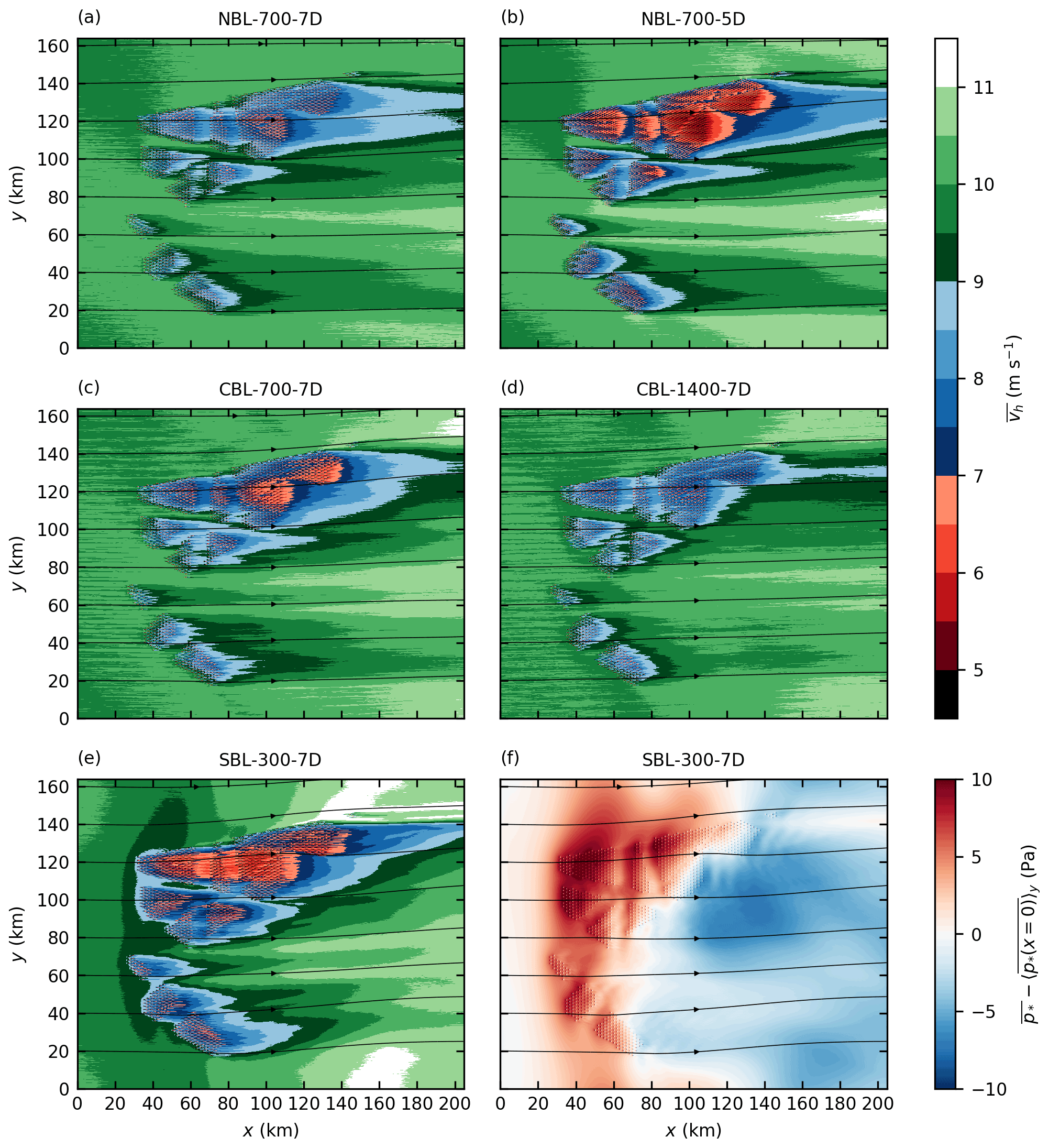
Figure 4 Mean horizontal wind speed $\stackrel{\mathrm{‾}}{v_{\mathrm{h}}}$ at hub height for all five cases (a–e) and perturbation pressure p_∗ at hub height relative to its value at the inflow for the case SBL-300-7D (f). Streamlines indicate the wind direction.

For the NBL cases, the wind speed is reduced from 10 to 7 m s⁻¹ for a turbine spacing of s=7 D and 5 m s⁻¹ for s=5 D inside the large wind farms in Zone 3. The wake length is defined as the distance between the wind farm trailing edge and the point at which the wind speed recovers to 90 % of its initial value, i.e., 9 m s⁻¹. For the small wind farms N-1, N-2 and N-3 (see Fig. 1), the wake length ranges from 1 to 20 km. However, the wake length of the large wind farms in Zone 3 is approximately 100 km for s=7 D, and the wake extends beyond the model domain for s=5 D.

The wake flow is deflected counterclockwise. The largest deflection angle of approximately 10^∘ is observed for the smaller turbine spacing (s=5 D). The counterclockwise wake deflection is consistent with the findings of Allaerts and Meyers (2016), who observed a counterclockwise deflection of 2–3^∘ for a 15 km long wind farm. A counterclockwise wind direction change (higher ageostrophic wind component) has also been observed by Abkar and Porté-Agel (2014) and Johnstone and Coleman (2012), who investigated infinitely large wind farms. The wake deflection is caused by a reduced Coriolis force, as is shown in the next section. Because the Coriolis force is proportional to the wind speed, the deflection angle is higher for the case with the greater speed deficit (NBL-700-5D). The reasons for the slow speed recovery and the wake deflection are discussed in detail in the next section.

The inflow wind speed has slight variations in the crosswise direction which are caused by the wind-farm-induced flow deceleration reaching the recycling plane (see Sect. 2.3). The variations have an amplitude of approximately 0.1 m s⁻¹, which is 1 % of the inflow wind speed.

For the CBL cases, the wind speed is reduced to 6.5 m s⁻¹ for h=700 m and 8 m s⁻¹ for h=1400 m inside the large wind farms in Zone 3. Also, the wake length of the large wind farms is much longer for the shallow BL than for the thick BL. This BL height dependency occurs because the turbulent vertical kinetic energy flux is greater for the case with the thicker BL (see Fig. 11c and d). The wind speed deficit and the wake length of small wind farms (e.g., N-1, N-2 and N-3) are relatively unaffected by the BL height because the wind-farm-induced internal BL does not reach the inversion layer (NBL cases) or only reaches it several tens of kilometers downstream of the wind farm trailing edge (CBL cases) (see Fig. 8). Consequently, the BL height only affects further wind speed recovery (e.g., to 9.5 m s⁻¹) in the far wake of small wind farms. For example, the wind speed recovery from 9 to 9.5 m s⁻¹ in the wake of N-2 takes longer for the case CBL-700-7D (40 km) than for the case CBL-1400-7D (15 km) (see Fig. 4c and d).

The wake is deflected counterclockwise in the CBL cases, as well. The deflection angle is approximately 5^∘ for the case with the shallow BL and 1–2^∘ for the case with the thick BL. The higher deflection angle for the case with the shallow BL is caused by a greater speed deficit compared to the case with the thick BL.

A comparison between the cases NBL-700-7D and CBL-700-7D shows that the speed deficit inside Zone 3 is greater for the CBL case. Also, the wakes of the small wind farms are longer for the CBL case. This is contradictory to the well-known fact that wind turbine and wind farm wakes are generally shorter in CBLs than in NBLs and SBLs (Porté-Agel et al., 2020, their Sects. 2.3 and 3.4.2). To achieve the same hub height wind speed for both cases, the geostrophic wind speed is 6 % greater for the NBL case (see Table 1) than for the case CBL-700-7D. Additionally, the wind speed is supergeostrophic in the upper half of the NBL, and thus the mean BL wind speed is approximately 10 % greater in the NBL case than in the CBL case. Stability likely has little-to-no effect because the stratification of the CBL case is only weakly unstable ($L=-\mathrm{420}$ m; see Table 1).

In the stable case SBL-300-7D, the wind speed is reduced to below 7 m s⁻¹ in the first 20 km of the large wind farms in Zone 3. The wind speed deficit is greater, and the wake is more than 20 km longer for the small wind farms compared to the other cases with s=7 D. The wake of the large wind farms in Zone 3, however, is not longer than in the cases NBL-700-7D and CBL-700-7D. This occurs because the speed recovery in the wake of this large wind farm is not driven by momentum flux divergence (which is stability dependent) but rather by a favorable pressure gradient (details are given in the next section). The case SBL-300-7D covers several flow features that are not as significant in the other cases. These features are namely flow blockage in front of the wind farms, flow deflection around the wind farms and flow acceleration beside the wind farms and/or wakes. These features are related to the pressure field inside and around the wind farms. The perturbation pressure $\stackrel{\mathrm{‾}}{p^{\ast }}$, relative to its value at the inflow, is shown in Fig. 4f. A high-pressure region in the upstream part of the large wind farms in Zone 3 leads to an adverse pressure gradient and thus flow deceleration in front of the wind farms. This effect is known as blockage effect or flow blockage (Wu and Porté-Agel, 2017). At a distance of 2.5 D upstream of the first wind turbine row of the wind farms in Zone 3, the wind speed is reduced by approximately 10 % relative to the inflow wind speed. For all other cases the speed reduction is approximately 2 %. Wu and Porté-Agel (2017) reported 11 % speed reduction 2.5 D upstream of the first turbine row of a 20 km long wind farm in a CNBL with a FA stratification of $\mathrm{\Gamma }=+\mathrm{5}$ K km⁻¹. However, for $\mathrm{\Gamma }=+\mathrm{1}$ K km⁻¹ they reported a speed reduction of only 1.2 % because the flow is supercritical (Froude number, Fr>1). Using the same definition² as in Wu and Porté-Agel (2017), the Froude number in the case SBL-300-7D is Fr=1.47, indicating a supercritical flow. This should, according to the reasoning of Wu and Porté-Agel (2017), result in a weak flow blockage, which does not correspond to the significant flow blockage observed in the case SBL-300-7D. The only case that is subcritical (and should thus show significant flow blockage) is CBL-1400-7D (Fr=0.81), but in this case the flow blockage is only very weak. Hence, for the cases that are investigated in this study, the Froude number, as defined by Wu and Porté-Agel (2017), is not an appropriate parameter for predicting flow blockage.

In the downstream part of the large wind farms, a favorable pressure gradient tends to accelerate the flow, counteracting the wind-turbine-induced flow deceleration. Consequently, the wind speed does not decrease further but remains nearly constant at approximately 6 m s⁻¹. In the wake, the pressure is more than 5 Pa smaller than the undisturbed pressure upstream of the wind farms. This results in a relatively fast speed recovery in the wake and in wind speeds well above the inflow wind speed beside the wakes. Note that this effect might be overestimated because the wind farms block a relatively large fraction of the domain width. The pressure perturbations are induced by large-scale gravity waves that are triggered by the wind farms. The observed pressure distribution in the streamwise direction is consistent with the findings of Allaerts and Meyers (2017) and Wu and Porté-Agel (2017), who investigated semi-infinite wind farms in CNBLs. The effect can only be seen in the case SBL-300-7D because it is most extreme if the BL height approaches the total height of the wind turbines. More details about wind-farm-induced gravity waves are provided in Sect. 3.1.4.

Because the wind farms in this study have a finite size also in the crosswise direction, it can be seen that the pressure perturbation also significantly affects the wind direction. Due to the streamwise reduction in wind speed, the flow diverges in the crosswise direction inside the wind farms. In the wake, where the flow accelerates, horizontal convergence can be observed.

3.1.2 Reasons for wake deflection and slow speed recovery

What is the reason for the slow speed recovery and the wake deflection inside and behind the large wind farms? In order to answer that question, Fig. 5 shows streamwise (parallel to streamlines) and crosswise (perpendicular to streamlines) components of the pressure gradient force³, the Coriolis force F_c and the resolved vertical turbulent momentum flux divergence, also called frictional force F_f, at z=150 m and y=120 km. The pressure gradient force can be divided into the geostrophic pressure gradient force F_gp, which is constant and is defined by the geostrophic wind, and the perturbation pressure gradient force F_pp, which can vary horizontally due to wind-farm-induced pressure perturbations. The forces are averaged over 1 turbine spacing along x and y in order to eliminate peaks in F_pp that are caused by single turbines. Thrust forces of the turbines are not included. The analysis is made from a Lagrangian frame of reference, examining the forces on an air parcel during its passage through the wind farms. From an Eulerian frame of reference, the sum of all forces, including the advection tendencies, would sum to zero because the flow is stationary.

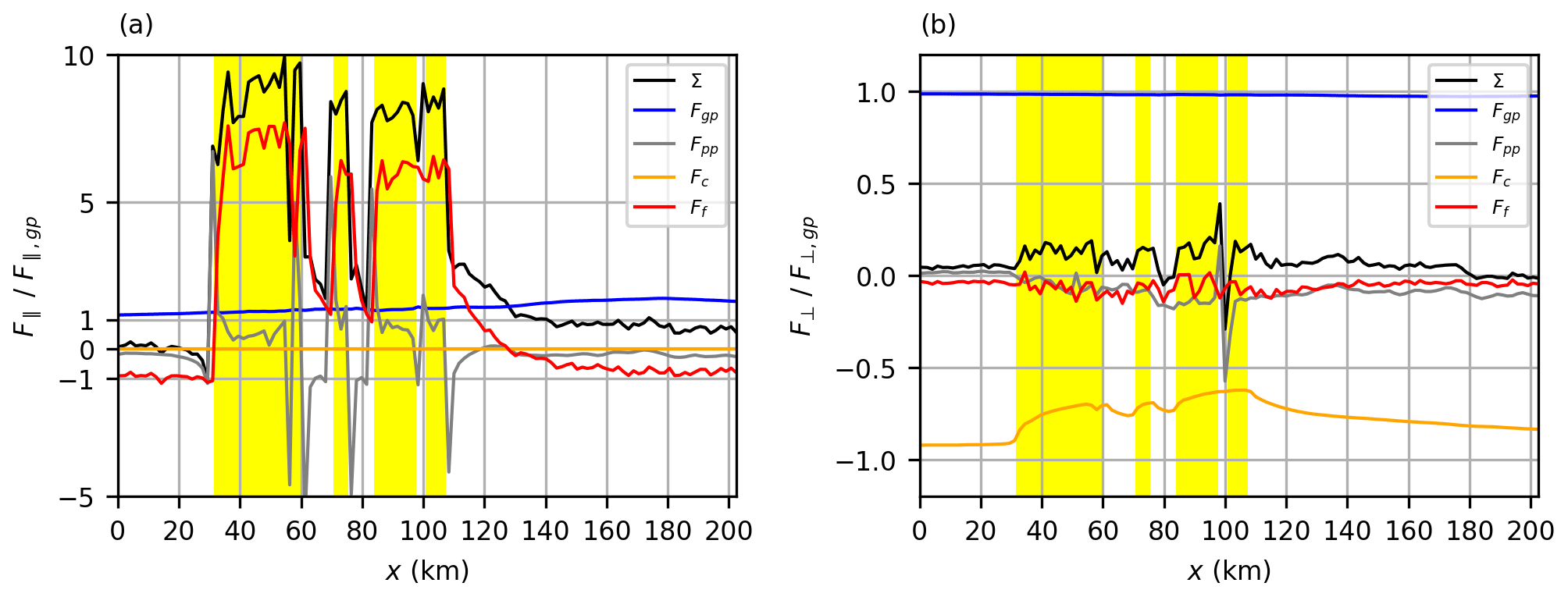
Figure 5 Streamwise and crosswise force components F_‖ (a) and F_⊥ (b) along a line at y=120 km and z=150 m for the case NBL-700-7D. Shown are the geostrophic pressure gradient force (F_gp), the perturbation pressure gradient force (F_pp), the Coriolis force (F_c), the frictional force (F_f, momentum flux divergence) and the sum of all forces (Σ). The forces are normalized by the respective geostrophic pressure gradient force component at the inflow and are horizontally averaged over one turbine spacing along x and y. The position of the wind farms is marked by yellow areas.

Streamwise force components in Fig. 5a show that the accelerating geostrophic pressure gradient force and the decelerating momentum flux divergence are in balance and sum to zero at the inflow. The streamwise component of the Coriolis force is zero because this force acts always perpendicular to the flow. Inside the wind farms, the momentum flux divergence is positive and thus is an accelerating component. It is the dominant driving force because it is more than 7 times greater than the geostrophic pressure gradient force.

An increasing perturbation pressure in front of the wind farm leads to a negative perturbation pressure gradient force and thus flow deceleration (often called blockage effect). However, inside the wind farms the perturbation pressure gradient force is positive due to a favorable pressure gradient (decreasing pressure). In the near wake the momentum flux divergence is high and leads to a fast speed recovery. The momentum flux divergence decreases fast until it becomes negative in the far wake so that the speed recovers slowly in the far wake. The only force that remains for driving the flow is the geostrophic pressure gradient force. At the inflow, this force is in balance with the momentum flux divergence, but in the wake this is not the case due to two reasons: first, the negative momentum flux divergence is weaker than at the inflow due to a lower wind speed and thus a reduced near-surface momentum flux; second, the streamwise component of the geostrophic pressure gradient force has increased by 80 % because the wake flow is deflected counterclockwise (i.e., to lower pressure). These results show that the wake deflection is an elementary feature of the wake that supports the wind speed recovery. They also show that mixing of momentum from the BL to the wind turbine level is not the dominant process that drives the speed recovery in the far wake of very large wind farms.

The wake deflection can be explained by examining the crosswise force components that are shown in Fig. 5b. Positive forces result in counterclockwise flow deflection, and negative forces result in clockwise flow deflection. At the inflow, the Coriolis force, the geostrophic pressure gradient force and the momentum flux divergence are in balance. Because the Coriolis force is proportional to the wind speed, it is reduced by approximately 30 % inside the wind farms and the wake. Consequently, the sum of all forces becomes positive and the flow is deflected counterclockwise. The momentum flux divergence and the perturbation pressure gradient force are negative inside the wind farm and inside the wake and are therefore opposing the wake deflection. The negative perturbation pressure gradient force is a result of the pressure distribution around the wind farms that is caused by the wind farm shape (see Fig. 4d).

The reason for the negative momentum flux divergence is the enhanced downward mixing of negative y momentum of the overlying flow, which veers to the right (see Fig. 3). For small wind farms this process can be dominant and may result in clockwise wake deflection (Van Der Laan and Nørmark Sørensen, 2017). However, for very large wind farms, as in this study, the effect of the reduced Coriolis force is dominant. An appropriate parameter for estimating the importance of Coriolis effects is the Rossby number. Coriolis effects become dominant for Rossby numbers close to or below 1. For the large wind farms in Zone 3 with a length of L_wf≈100 km at mid-latitudes (Coriolis parameter $f\approx {\mathrm{10}}^{-\mathrm{4}}$) and a wind speed of U≈10 m s⁻¹, the Rossby number becomes

$$\begin{array}{}\text{(11)}& Ro={\displaystyle \frac{U}{L_{\mathrm{wf}}f}}\approx \mathrm{1},\end{array}$$

indicating that Coriolis effects play an important role for flows in wind farms of this size.

3.1.3 Turbulence intensity at hub height

The turbulence intensity TI is defined as in Porté-Agel et al. (2013):

$$\begin{array}{}\text{(12)}& \mathrm{TI}={\displaystyle \frac{\sqrt{\frac{\mathrm{2}}{\mathrm{3}}\mathrm{TKE}}}{\stackrel{\mathrm{‾}}{v_{\mathrm{h}}}}},\end{array}$$

where TKE is the resolved turbulence kinetic energy defined as follows:

$$\begin{array}{}\text{(13)}& \mathrm{TKE}={\displaystyle \frac{\mathrm{1}}{\mathrm{2}}}(\stackrel{\mathrm{‾}}{{u^{\prime }}^{\mathrm{2}}}+\stackrel{\mathrm{‾}}{{v^{\prime }}^{\mathrm{2}}}+\stackrel{\mathrm{‾}}{{w^{\prime }}^{\mathrm{2}}}),\end{array}$$

where $\stackrel{\mathrm{‾}}{{u^{\prime }}^{\mathrm{2}}}$, $\stackrel{\mathrm{‾}}{{v^{\prime }}^{\mathrm{2}}}$ and $\stackrel{\mathrm{‾}}{{w^{\prime }}^{\mathrm{2}}}$ are the resolved-scale variances of u, v and w, respectively. The SGS-TKE is neglected because it is smaller than 10 % of the resolved TKE inside the wind turbine wakes at a distance of 3 D or more.

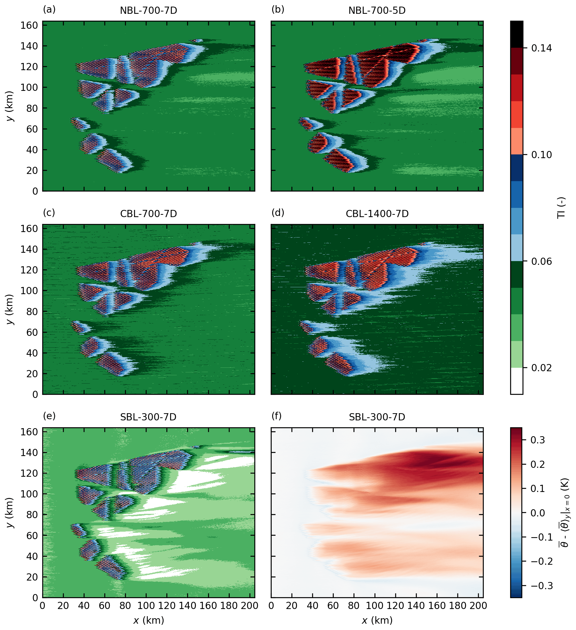
Figure 6 Turbulence intensity (TI) at hub height for all five cases (a–e) and potential temperature at hub height relative to the inflow temperature for the case SBL-300-7D (f).

The TI at hub height is shown in Fig. 6. Inside the wind farms, the TI reaches a fully developed state after approximately four rows and is constant farther downstream. A smaller turbine spacing leads to a greater TI inside the wind farms. For the case NBL-700-7D, a TI of 10 % is reached inside the wind farms, but more than 14 % is reached in the case NBL-700-5D. In the CBL cases, the TI inside the wind farms reaches 10 % in case CBL-700-7D and approximately 12 % in CBL-1400-7D. Although the ambient TI is only approximately 3 % for the case SBL-300-7D, the TI inside the wind farms reaches values similar to NBL-700-7D (approximately 10 %).

The wake in terms of TI is generally shorter than the wake in terms of wind speed (see Fig. 4). The shortest wakes occur in the shallow SBL (SBL-300-7D), and the longest wakes occur in the thick CBL (CBL-1400-7D). This is the opposite behavior than that of the wake in terms of wind speed. The wake length in terms of TI weakly depends on wind farm size with slightly longer wakes for larger wind farms. However, this effect is caused by the definition of the TI, in which the wind speed variances are normalized by the mean horizontal wind speed. The mean horizontal wind speed is smaller in the wake of the large wind farms than in the wake of the small wind farms, resulting in a higher TI in the wake of the large wind farms. The wind farm size dependency of the wake length vanishes if the TKE is used for measuring the wake length instead of the TI (not shown).

In the NBL cases and especially in the SBL case, the TI in the far wake drops below the ambient TI at the inflow. This effect is caused by the reduced wind speed in the far wake which leads to a reduction in the shear-driven turbulence production. In the CBL cases, there is also buoyancy-driven turbulence production, which is unaffected by the reduced wind speed in the wake and thus maintains the TI level. That buoyancy-driven turbulence production has a large impact on hub height TI is also verified by the fact that the ambient TI is greater in the CBL case with the thick BL (CBL-1400-7D) than in the case with the shallow BL (CBL-700-7D): the convective velocity scale $w^{\ast }=\left(\frac{g{z}_{\mathrm{i}}}{\stackrel{\mathrm{‾}}{\mathit{\theta }}}\right(\stackrel{\mathrm{‾}}{w^{\prime }{\mathit{\theta }}^{\prime }}{)}_{\mathrm{0}}{)}^{\mathrm{1}/\mathrm{3}}$ is greater in the case CBL-1400-7D than in the case CBL-700-7D, and hence also the buoyancy-generated velocity variances are greater. Because buoyancy acts as a TKE sink in the SBL case, it can not compensate for the reduction in shear-driven turbulence production, and thus the TI in the wake drops below 2 %. This effect is amplified by the entrainment of warm air into the BL that leads to a stabilization (increased lapse rate) at hub height and therefore stronger turbulence damping (see Figs. 6f and 9). The entrainment of warm air results in a temperature increase at hub height of approximately 0.3 K for the large wind farms and approximately 0.1 K for the small wind farms.

3.1.4 Boundary layer development

Figure 7 shows vertical cross sections of the horizontal mean wind speed for all cases. The cross sections are located at y=120 km and thus cross the large wind farms in Zone 3. The inversion layer height z_i is marked by lines at which the maximum vertical potential temperature gradient occurs. The wind-farm-induced internal boundary layer (IBL) is shown by a line at which the horizontal wind speed corresponds to 97 % of the inflow wind speed at that height.

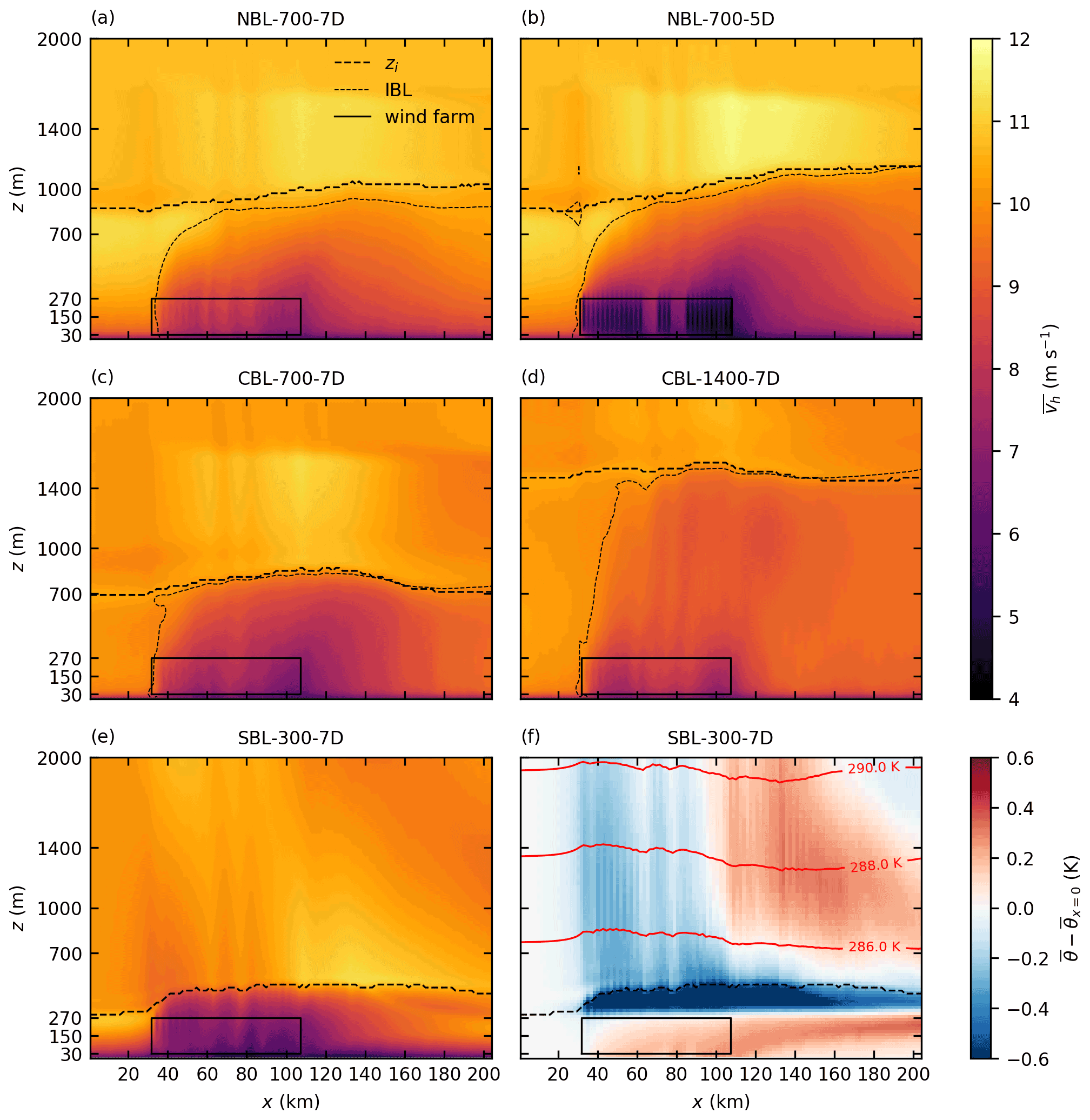
Figure 7 Vertical cross sections at y=120 km of wind speed v_h for all cases (a–e) and potential temperature deviation relative to the inflow temperature for the case SBL-300-7D (f). Also shown are the inversion layer height z_i (maximum vertical temperature gradient), the internal boundary layer IBL (97 % of inflow wind speed) and the extent of the wind farms in Zone 3.

The IBL is not shown for the case SBL-300-7D because the wind turbines are nearly as high as the BL. For all other cases the IBL grows up to the inversion layer (IL) within 40 km (NBL-700-7D and NBL-700-5D), 10 km (CBL-700-7D) and 20 km (CBL-1400-7D) behind the wind farm leading edge. The streamwise extent of the IBL goes beyond the model domain, indicating that the wind speed inside the entire BL does not recover to 97 % of the inflow wind speed.

The IL height is affected by the presence of the wind farms in all five cases. In the NBL cases the IL is displaced upwards by 200–300 m, whereas a larger displacement occurs for the smaller turbine spacing. The IL displacement is a result of the reduced wind speed in the bulk of the BL: to obtain a divergence-free flow inside the BL, the wind speed reduction (streamwise convergence) is compensated for by vertical divergence (IL displacement) and crosswise divergence (flow around the wind farms). The increase in IL height is not caused by entrainment of warm air into the BL (as can also be seen in the profiles of potential temperature in Fig. 9). This phenomenon has also been observed by Allaerts and Meyers (2017), who also stated that the mass flux conservation is the reason for the IL displacement. Abkar and Porté-Agel (2014) stated that a smaller turbine spacing results in a larger BL height for an infinite wind farm in a CNBL. The IL displacement causes an acceleration of the flow in the FA for the NBL and CBL cases. Details about this effect are described in the next section.

In the CBL cases, the IL height increases above the wind farms and decreases above the wake, reaching its initial value at approximately 70 km downstream of the last wind farm trailing edge. The IL displacement is larger for the shallower BL, i.e., the case CBL-700-7D.

The IL displacement is most significant for the case SBL-300-7D. The IL height increases from 300 to 500 m. Allaerts and Meyers (2016) also reported that larger IL displacements occur for shallower BLs (+60 % for h=250 m). In the case SBL-300-7D, the IL height increase is caused by vertical displacement due to mass conservation and also by entrainment of warm air into the BL (see Fig. 7f). The entrainment of warm air into the BL leads to a warming of the lower part of the BL. However, the temperature at the height of the original IL is reduced because the warm air in the IL is replaced by relatively cold air from the BL.

Because the laminar flow in the FA is adiabatic, the isotherms in Fig. 7f can be interpreted as streamlines. They show that gravity waves are excited by the wind farms. There are small-scale gravity waves with a wavelength that corresponds to the turbine spacing and a large-scale gravity wave with a wavelength that approximately corresponds to the wind farm length. The negative and positive temperature deviations in the wave crest and trough, respectively, cause a positive and negative deviation in the perturbation pressure at the surface, as is shown in Fig. 4f. A detailed analysis of the wind-farm-induced gravity waves goes beyond the scope of this study. However, it is noted that the qualitative pressure and temperature distributions correspond to the findings of Allaerts and Meyers (2017) and Wu and Porté-Agel (2017).

Additional test simulations have shown that the strength of the gravity waves is sensitive to the domain height. Allaerts and Meyers (2017) achieved good results (low wave reflection at the domain top) if the domain height corresponds to at least one vertical wavelength ${\mathit{\lambda }}_z=\mathrm{2}\mathit{\pi }U/N$, where U is the BL bulk wind speed, and N is the Brunt–Väisälä frequency in the FA. In the case SBL-300-7D, the domain height is set to 0.43λ_z (λ_z=5.9 km, L_z=3624 m) because larger domain heights lead to numerical instabilities at the inflow. Wu and Porté-Agel (2017) used a domain height of L_z=2.4 km for a FA stratifications of Γ=1 K km⁻¹ (resulting in L_z=0.22λ_z) and Γ=5 K km⁻¹ (resulting in L_z=0.49λ_z). It is not clear whether the vertical wavelength is the only relevant parameter for choosing the correct domain height or whether the wind farm length also has to be considered. Further research is needed to find setup guidelines that ensure that wind-farm-induced gravity waves are covered as realistically as possible.

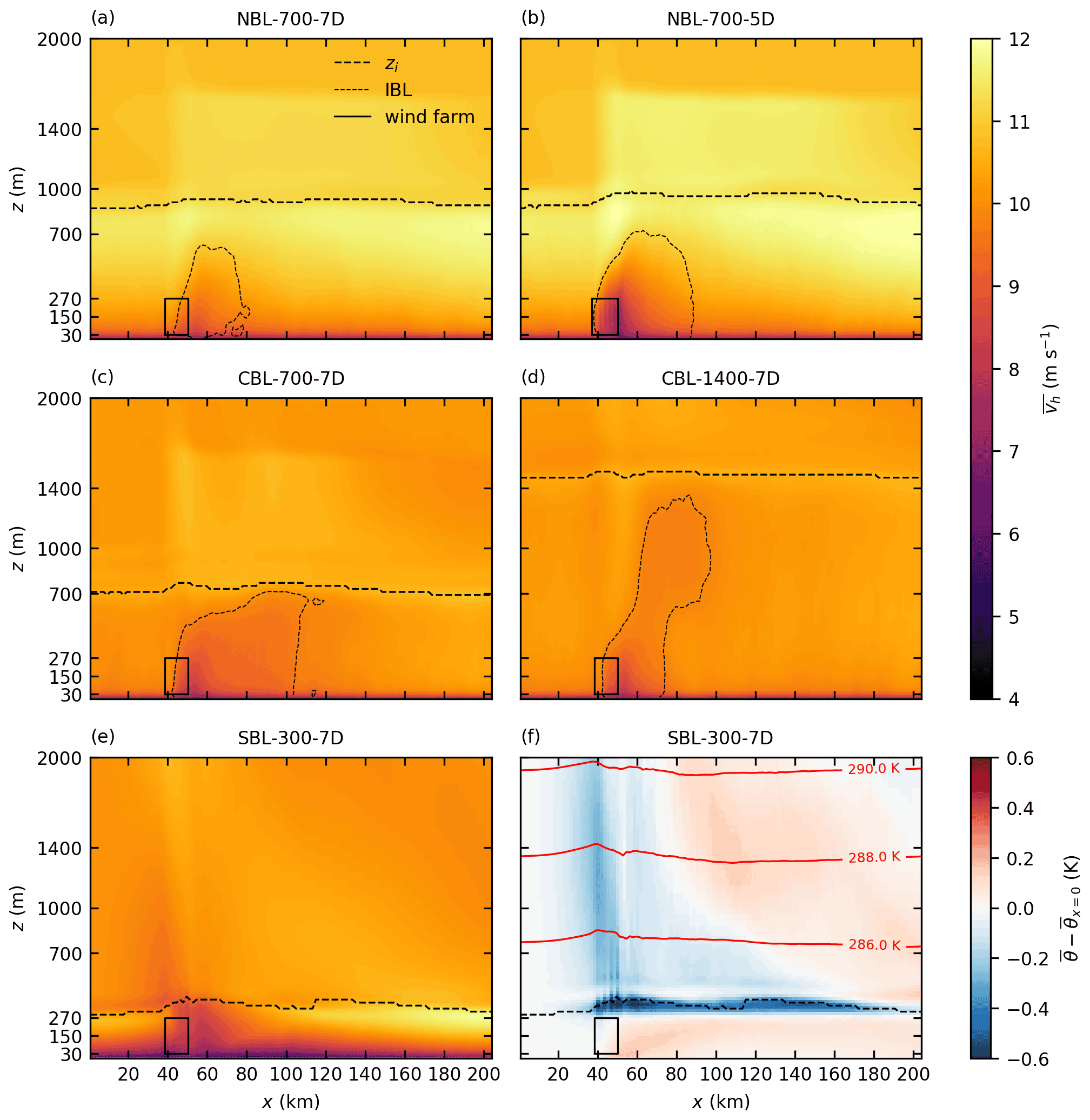
Figure 8 Vertical cross sections at y=50 km of wind speed v_h for all cases (a–e) and potential temperature deviation relative to the inflow temperature for the case SBL-300-7D (f). Also shown are the inversion layer height z_i (maximum vertical temperature gradient), the internal boundary layer IBL (97 % of inflow wind speed) and the extent of the wind farm N-2.

In order to compare the effects of small and large wind farms on the boundary layer, Fig. 8 shows vertical cross sections at y=50 km, crossing the small wind farm N-2. The IL displacement is much smaller compared to the displacement triggered by the large wind farms (i.e., 50–100 m for the small wind farm in contrast to 200–300 m for the large wind farms). For the NBL cases the IBL grows to approximately 700 m and thus does not reach the IL. For the case CBL-700-7D the IBL reaches the IL but only 40 km behind the wind farm trailing edge. The streamwise extent of the IBL shows that the wind speed recovery at hub height to 97 % of the inflow wind speed is reached 20 km (NBL-700-7D and CBL-1400-7D) and approx. 50 km (NBL-700-5D and CBL-700-7D) behind the wind farm trailing edge. For all 7 D cases, the IBL does not start at the wind farm leading edge but rather inside the wind farms. The reason for this effect is that the vertical cross section does not cross the rotor discs of the turbines, and no averaging occurs in the y direction. As Fig. 8f shows, the small wind farms also triggers gravity waves in the FA, but they are much weaker than the ones triggered by the large wind farms.

3.1.5 Profiles of wind speed, wind direction and potential temperature in the wake

To examine the effect of the wind farms on the BL in more detail, profiles of wind speed, wind direction and potential temperature are shown in Fig. 9. The profiles are evaluated at the inflow (x=0 km), in the near wake (x=120 km) and in the far wake (x=180 km) of the large wind farms in Zone 3 (y=120 km).

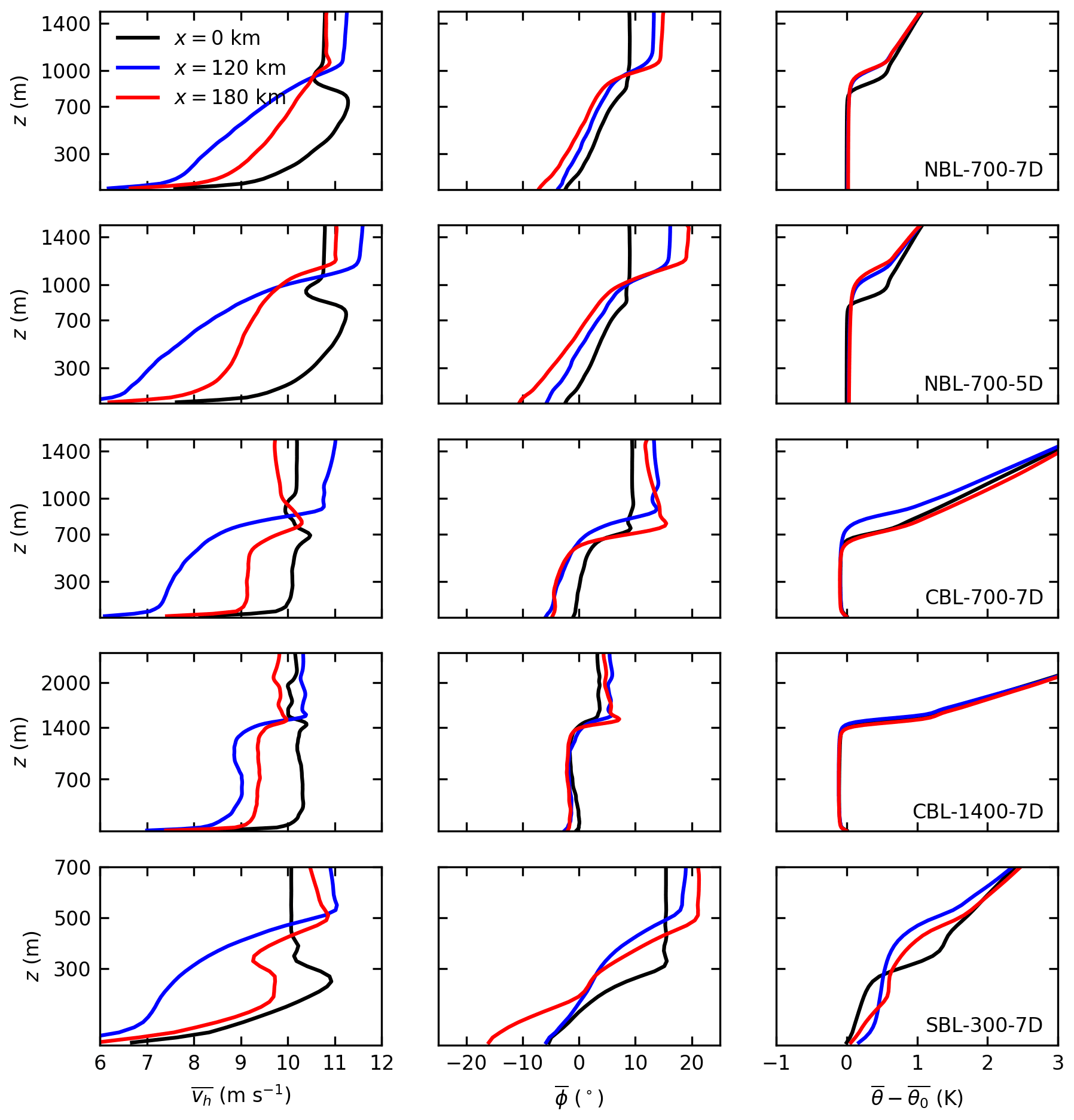
Figure 9 Vertical profiles of temporal averaged horizontal wind speed ($\stackrel{\mathrm{‾}}{v_{\mathrm{h}}}$), wind direction ($\stackrel{\mathrm{‾}}{\mathit{\varphi }}$, clockwise positive) and potential temperature ($\stackrel{\mathrm{‾}}{\mathit{\theta }}$) relative to surface temperature $\stackrel{\mathrm{‾}}{{\mathit{\theta }}_{\mathrm{0}}}$ at the inflow (x=0 km), in the near wake (x=120 km) and in the far wake (x=180 km) of the large wind farms in Zone 3 (y=120 km) for all five cases. The wind farm trailing edge is located at x=108 km.

The wind speed profiles show that the wind-farm-induced wind speed deficit spreads over the entire height of the BL. The effective vertical mixing in the CBL cases results in an approximately height-constant wind speed at the inflow and in the wake. In the case CBL-1400-7D, the wind speed in the upper part of the BL is even lower than in the lower part of the BL at x=120 km. In the NBL cases, the vertical mixing is not as effective, and thus a significant wind shear exists over the entire BL in the wake. The wind speed profiles of the case SBL-300-7D show that the BL has grown from 300 to 500 m and that the super-geostrophic maximum is eliminated completely. The IL displacement causes an increase in wind speed in the FA above the BL. The maximum increases (approximately 1 m s⁻¹) are observed for the cases with the greatest IL displacements. That suggests that the wind speed excess above the BL is also caused by the continuity constraint; i.e., the wind speed has to increase in order to maintain a constant mass flux between the IL and the domain top. For the CBL cases, in which the IL height decreases again behind the wind farms, the wind speed above the BL decreases to below-geostrophic in the far wake (x=180 km). Note that these effects could be overestimated because of the artificial boundary that is introduced by the Rayleigh damping layer that starts several hundred meters above the BL. The sensitivity of this effect on the Rayleigh damping height has not been investigated because the scope of this study is on BL-internal effects.

The wake deflection shown in the horizontal cross sections can also be seen in the wind direction profiles. The wind-farm-induced wind direction change is approximately constant over the entire height of the BL. The largest deflection angles of up to −10^∘ are observed for the cases with the greatest speed deficit (SBL-300-7D and NBL-700-5D) because the Coriolis force reduction is greatest in these cases. The smallest deflection angle is observed in the case CBL-1400-7D with no deflection in the upper half of the BL. All cases have in common that, in contrast to the counterclockwise deflection in the BL, the flow in the FA is deflected clockwise. As a result, the wind veer in the inversion layer increases to approximately 10^∘. The flow deflection in the FA is also a Coriolis effect. Because the wind speed in the FA is supergeostrophic, the Coriolis force is greater than the geostrophic pressure gradient force, and therefore the flow is deflected clockwise. The largest deflection angle of more than 10^∘ is observed for the case NBL-700-5D. Note that the highest wind speed excess occurs at x=120 km, but the highest deflection angle occurs at x=180 km. This effect can be interpreted as an inertia oscillation in space (along x), with the deflection angle being phase shifted 90^∘ relative to the wind speed excess. Note that this effect might also be overestimated due to the potentially overestimated wind speed excess. However, currently running investigations with much higher Rayleigh damping heights show the same behavior. In the case SBL-300-7D, the combination of clockwise deflection in the FA and counterclockwise deflection in the BL results in a total wind veer of approximately 40^∘ between the surface and the FA.

The effect of the wind farms on the potential temperature profiles is largest for shallow BLs (SBL-300-7D) and negligibly small for thick BLs (CBL-1400-7D). The potential temperature profiles inside the well-mixed BLs of the NBL and CBL cases are nearly unaffected by the wind farms. The greatest changes take place in the inversion layer, which is displaced upwards in order to maintain a constant mass flux in the BL, as already described in the previous section. The profiles show that the potential temperature inside the BL is unchanged, and thus BL warming due to entrainment of warm air from the FA is not the reason for the increased IL height. On the contrary, the temperature at the height of the original IL decreases by approximately 0.5 K because it is replaced by colder air from the underlying BL. The potential temperature profile of the SBL case is heavily modified by the wind farms. The temperature in the BL increases by approximately 0.5 K due to entrainment of warm air from the FA into the BL. The IL rises from 300 to 500 m due to the combined effect of BL warming and IL displacement. Because the surface temperature is constant, a new SBL forms in the far wake. This new SBL is shallower and more stably stratified than the original SBL at the inflow.

3.2 Power output

3.2.1 Wind turbine and wind farm efficiencies

The effect of different turbine spacings, BL heights and stabilities on the power output of very large wind farms is investigated here. This is done by comparing wind farm efficiencies of small and large wind farms for the five simulated cases. Here, the turbines in the area N-1 are defined as a small wind farm because this area has the size of a typical, currently existing wind farm in the German Bight. The turbines in Zone 3 are defined as a large wind farm because this area will be equipped with wind farms in the future (see Fig. 10f). The small wind farm consists of 27 wind turbines for s=7 D and 54 wind turbines for s=5 D, resulting in an installed wind farm capacity of 0.405 GW for s=7 D and 0.810 GW for s=5 D. The large wind farm consists of 636 wind turbines for s=7 D and 1260 wind turbines for s=5 D, resulting in an installed wind farm capacity of 9.54 GW for s=7 D and 18.90 GW for s=5 D.

The wind farm efficiency η_wf is defined as the total wind farm power P_wf normalized by the wind farm power that would be achieved if all wind turbines n_wt were operating in free-stream conditions, generating the reference power P_ref (all quantities are averaged over the last 4 h of the simulation):

$$\begin{array}{}\text{(14)}& {\mathit{\eta }}_{\mathrm{wf}}={\displaystyle \frac{P_{\mathrm{wf}}}{n_{\mathrm{wt}}{P}_{\mathrm{ref}}}}.\end{array}$$

For each of the five cases the reference power is obtained by an additional simulation of a single turbine using the same inflow profiles as for the respective main simulation. The reference powers for each case are given in Table 2. The wind farm efficiency can also be interpreted as the wind turbine efficiency averaged over all wind turbines of the wind farm. The wind turbine efficiency of a wind turbine generating P_wt is defined as follows:

$$\begin{array}{}\text{(15)}& {\mathit{\eta }}_{\mathrm{wt}}={\displaystyle \frac{P_{\mathrm{wt}}}{P_{\mathrm{ref}}}}.\end{array}$$

The wind farm efficiencies of the small and the large wind farm are listed in Table 2, and the wind turbine efficiencies are shown in Fig. 10.

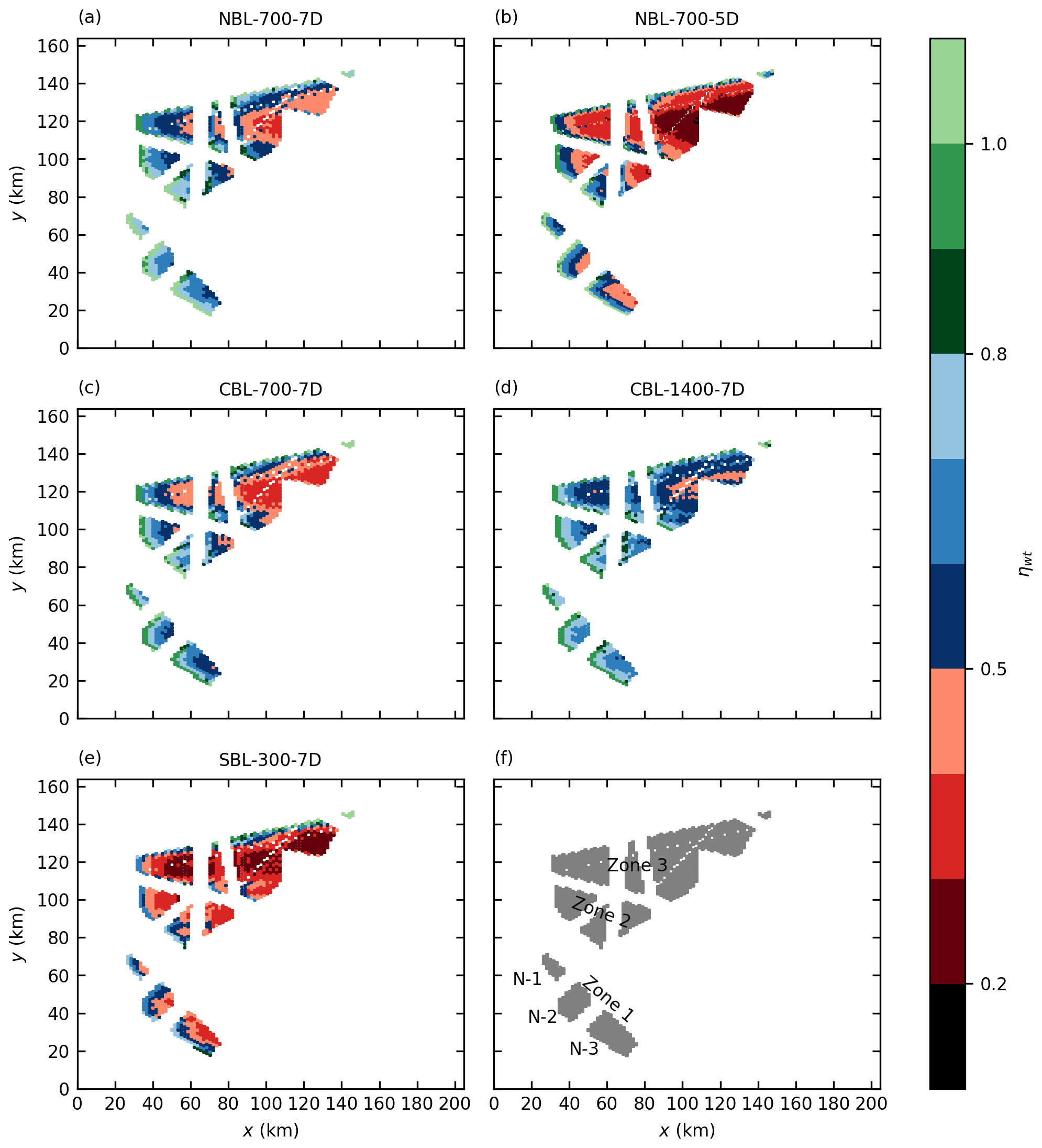
Figure 10 Wind turbine efficiencies η_wt for all five cases (a–e) and overview of wind farm names (f).

Table 2 Reference power of a single turbine in free-stream conditions and wind farm efficiencies for a small wind farm (N-1) and a large wind farm (Zone 3) for all five cases.

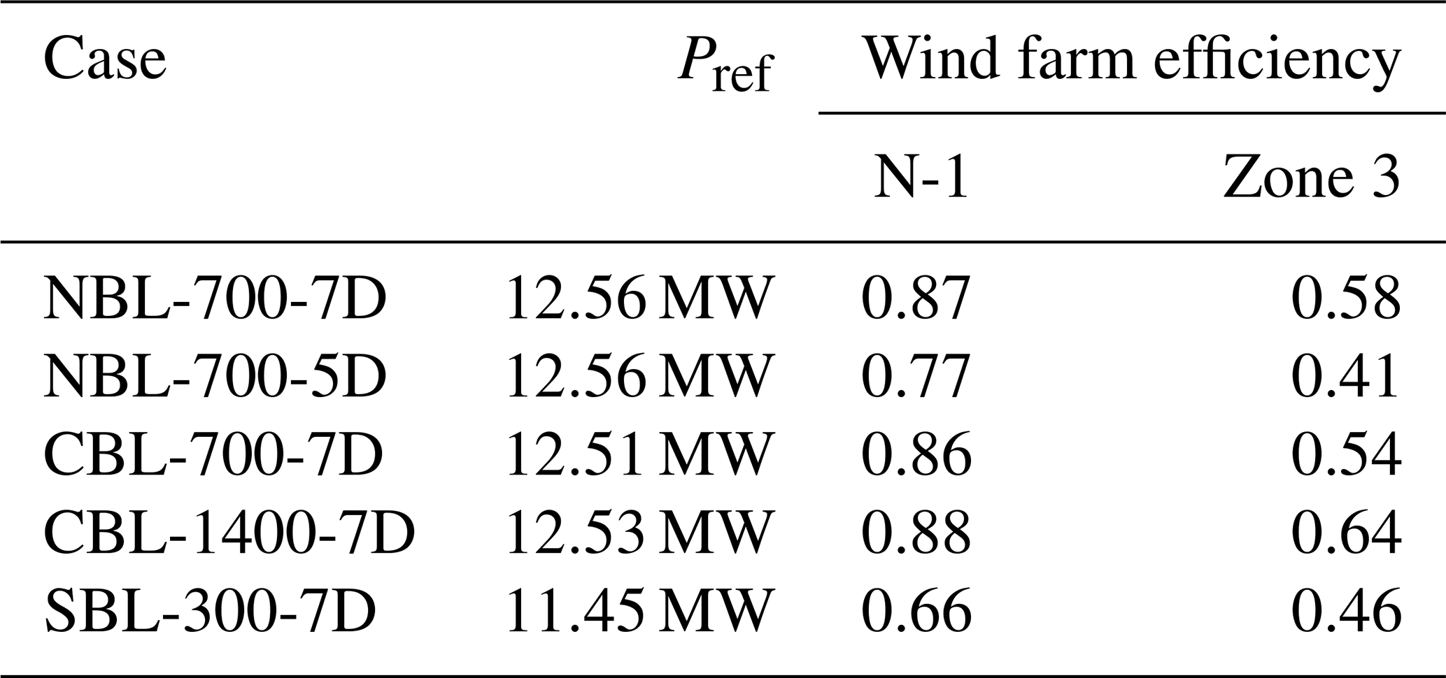
In general, the wind farm efficiency is significantly lower for large wind farms than for small wind farms. All 7D cases, except for the SBL case, show efficiencies of 0.86–0.88 for the small wind farm and efficiencies of 0.54–0.64 for the large wind farm. In the SBL case, the efficiency of the small wind farm is 0.66 because the wind farm is affected by the blockage effect of the sum of all wind farms. This is visible in Fig 10e, which shows that the efficiency of the wind turbines in the first row of N-1 is already below 0.8. The efficiency of the large wind farm is 30 % lower than that of the small wind farm for the SBL case. The blockage effect redistributes energy from upstream parts of the wind farm to downstream parts of the wind farm by a favorable pressure gradient, which has already been shown by Allaerts and Meyers (2017) for wind farms in shallow CNBLs. This effect can also be seen in the power distribution inside the farm: the turbine power is constant from approximately row 10 up to the trailing edge of the large wind farm in Zone 3 (see Figs. 10e and 11e). In all other cases the wind turbine power does not reach a steady state until the end of the wind farms.

A reduction of turbine spacing from s=7 D to s=5 D results in an efficiency reduction of 12 % (0.87 to 0.77) for the small wind farm but results in an efficiency reduction of 29 % (0.58 to 0.41) for the large wind farm. The low wind farm efficiency for the case NBL-700-5D can be explained by a fast drop in the turbine efficiencies to values below 0.4 only 20 km downstream of the leading edge. The low wind turbine efficiencies are caused by a reduction in the vertical kinetic energy flux, as shown in the next section.

A doubling of the BL height results in an efficiency increase of +2 % (from 0.86 to 0.88) for the small wind farm but in an efficiency increase of 19 % (from 0.54 to 0.64) for the large wind farm. The dependency of wind farm efficiency on the BL height has also been observed by Allaerts and Meyers (2016), who reported a 17.6 % increase in power deficit for a BL height reduction from 1000 to 250 m.

A comparison between the cases NBL-700-7D and CBL-700-7D shows that greater wind farm efficiencies are obtained for the NBL, although better efficiencies are expected for the CBL due to the better vertical mixing. Comparing the wind speed profiles of these cases (see Fig. 3) shows that the inflow wind speed in the bulk of the BL is higher for the NBL than for the CBL, which is probably the reason for the higher wind farm efficiencies. This result shows that it is important to consider not only the wind speed at hub height but also the wind profile inside the entire BL to make accurate wind farm performance predictions.

3.2.2 Energy source analysis

To examine the dependency of the wind farm efficiency on the turbine spacing and the BL height in more detail, an energy source analysis is made in this section. Here, an energy source is defined as an energy input to the flow, i.e., a process that drives the wake recovery. This can be one of the following:

1. vertical turbulent flux of kinetic energy at rotor top level, W_vkef;

2. work done by the geostrophic pressure gradient on the flow below rotor top level (bottom of the BL), W_gpg,wt;

3. work done by the perturbation pressure gradient on the flow below rotor top level, W_ppg,wt.

The analysis is a simplified version of the analyses made by Abkar and Porté-Agel (2014) and Allaerts and Meyers (2017) and does not claim to be a complete energy budget analysis. The intention of this analysis is to show which processes dominate the wake recovery and thus limit the achievable power density of very large wind farms. Thus the advection of upstream kinetic energy is not considered here. The above-named sources are calculated as follows.

The resolved downward turbulent flux of mean kinetic energy at rotor top level, averaged between $y=\mathrm{120}\mathrm{km}-s_y$ and $y=\mathrm{120}\mathrm{km}+s_y$, is calculated by multiplying the shear stress by the corresponding wind velocity component at that height:

$$\begin{array}{}\text{(16)}& W_{\mathrm{vkef}}\left(x_i\right)=\langle -\mathit{\rho }(\stackrel{\mathrm{‾}}{u}\stackrel{\mathrm{‾}}{w^{\prime }{u}^{\prime }}+\stackrel{\mathrm{‾}}{v}\stackrel{\mathrm{‾}}{w^{\prime }{v}^{\prime }}){|}_{z=z_t}{\rangle }_y.\end{array}$$

The power density of the energy input by the geostrophic pressure gradient on the flow below rotor top level z_t=270 m is calculated as follows:

$$\begin{array}{}\text{(17)}& W_{\mathrm{gpg},\mathrm{wt}}\left(x_i\right)=\underset{z=\mathrm{0}}{\overset{z_t}{\int }}\mathit{\rho }{f}_c\left(u_{\mathrm{g}}\stackrel{\mathrm{‾}}{v}\right(z)-v_{\mathrm{g}}\stackrel{\mathrm{‾}}{u}(z\left)\right)\mathrm{d}z{|}_{y=\mathrm{120}\mathrm{km}}.\end{array}$$

The work done by the geostrophic pressure gradient on the rest of the BL (between z_t and z_i) is calculated as follows:

$$\begin{array}{}\text{(18)}& W_{\mathrm{gpg},\mathrm{BL}}\left(x_i\right)=\underset{z=z_t}{\overset{z_{\mathrm{i}}}{\int }}\mathit{\rho }{f}_c\left(u_{\mathrm{g}}\stackrel{\mathrm{‾}}{v}\right(z)-v_{\mathrm{g}}\stackrel{\mathrm{‾}}{u}(z\left)\right)\mathrm{d}z{|}_{y=\mathrm{120}\mathrm{km}}.\end{array}$$

The power density of the energy input by the perturbation pressure gradient on the flow below rotor top level is calculated as follows:

$$\begin{array}{}\text{(19)}& W_{\mathrm{ppg},\mathrm{wt}}\left(x_i\right)=-\underset{z=\mathrm{0}}{\overset{z_t}{\int }}{\displaystyle \frac{\partial p^{*}\left(z\right)}{\partial x}}\stackrel{\mathrm{‾}}{u}\left(z\right)+{\displaystyle \frac{\partial p^{\ast }\left(z\right)}{\partial y}}\stackrel{\mathrm{‾}}{v}\left(z\right)\mathrm{d}z{|}_{y=\mathrm{120}\mathrm{km}}.\end{array}$$

The power densities of the wind turbines are defined as follows:

$$\begin{array}{}\text{(20)}& W_{\mathrm{wt}}={\displaystyle \frac{P_{\mathrm{wt}}}{s_x{s}_y}}.\end{array}$$

The power densities are shown in Fig. 11. For the case NBL-700-7D it can be seen that the first-row wind turbines operate at the reference power so that a high power density of $W_{\mathrm{wt}}=\mathrm{12.56}\mathrm{MW}/(\mathrm{7}\mathrm{D}{)}^{\mathrm{2}}=\mathrm{4.45}\mathrm{W}{\mathrm{m}}^{-\mathrm{2}}$ is achieved. The dominant energy source for the first turbine rows is the advection of kinetic energy. The advection is not included in Fig. 11 because it is larger than the other terms and would make the quantification of the smaller terms difficult. The power density of downstream wind turbines is determined by the vertical kinetic energy flux. Because the vertical kinetic energy flux decays from 3 W m⁻² at the beginning of the first wind farm to 2 W m⁻² at the end of the last wind farm, the power density of the wind turbines also decays to below 2 W m⁻². The good correlation between the wind turbine power density and the vertical kinetic energy flux has also been found by Stevens et al. (2016) for the fully developed regime in a 9 km long wind farm. The work done by the geostrophic pressure gradient on the flow below the rotor top level achieves a power density of approximately 0.6 W m⁻². It is thus not the dominating energy source inside the wind farms, but it still contributes approximately 20 % to the sum of all sources $W_{\mathrm{total}}=W_{\mathrm{vkef}}+W_{\mathrm{gpg},\mathrm{wt}}+W_{\mathrm{ppg},\mathrm{wt}}$. In the downstream half of the wind farms the ratio between the wind turbine power and W_total is approximately 70 %.

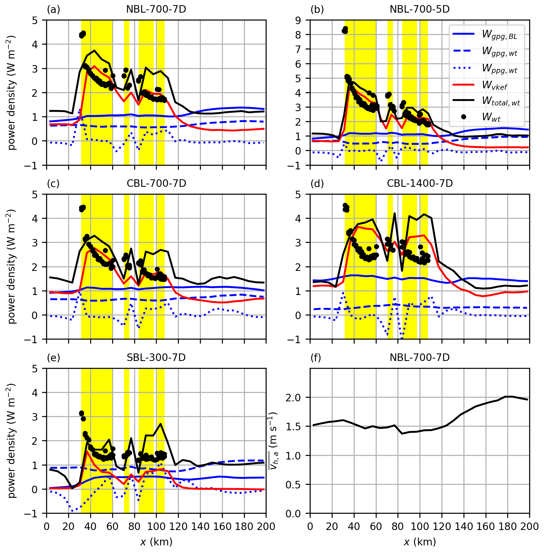
Figure 11 Comparison of power density provided by the geostrophic pressure gradient below rotor top level W_gpg,wt and above rotor top level W_gpg,BL, the perturbation pressure gradient below rotor top level W_ppg,wt, the vertical kinetic energy flux at rotor top level W_vkef, and W_total,wt as the sum of W_gpg,wt, W_ppg,wt and W_vkef. The power density of the wind turbines located between $y=\mathrm{120}-s_y$ and $y=\mathrm{120}+s_y$ is shown for comparison. Wind farm locations are marked by yellow areas. Panel (f) shows the ageostrophic wind speed component ($\stackrel{\mathrm{‾}}{v_{h,a}}$) at hub height for the case NBL-700-7D at y=120 km.

Although the vertical kinetic energy flux does not reach a constant value until the end of the wind farms, it is likely that it approaches the power density of the work done by the pressure gradient on the BL flow above the wind turbine level W_gpg,BL. Therefore, the flow approaches the fully developed regime of an infinite wind farm flow, in which all the energy extracted by the wind turbines is provided by the work done by the geostrophic pressure gradient on the BL flow (Johnstone and Coleman, 2012; Abkar and Porté-Agel, 2014).

The energy input by the geostrophic pressure gradient into the entire BL ($W_{\mathrm{gpg},\mathrm{wt}}+W_{\mathrm{gpg},\mathrm{BL}}$) achieves power densities of only 1–2 W m⁻², which is consistent with the geophysical limits to power densities of large wind farms found by Antonini and Caldeira (2021), who reported approximately 1.5 W m⁻² for a latitude of 46^∘ and a geostrophic wind speed of 12 m s⁻¹. This power density is much smaller than the power density achieved by the first-row wind turbines. As the case NBL-700-5D shows (Fig. 11b), a reduction of the turbine spacing from s=7 D to s=5 D approximately results in a doubling of the power density of the first-row wind turbines (from 4.5 to 8.5 W m⁻²), but the power density of the last-row wind turbines is as low as for s=7 D. This result indicates that the turbine spacing for very large wind farms should be chosen to be much larger than for small wind farms to achieve a good wind farm efficiency. That the wind farm power output is limited by the vertical kinetic energy flux has also been found by Badger et al. (2020), who investigated potential wind farm scenarios in the German Bight using a mesoscale weather forecast model (WRF) and a simple box model (KEBA, kinetic energy budget of the atmosphere). Nishino (2013) used a simple, theoretical approach to show that the power density of very large wind farms is limited by the energy input of the pressure gradient and that the power density is proportional to τ₀U_h, where τ₀ is the shear stress near the surface, and U_h is the mean wind speed at hub height for an undisturbed flow without wind farms. However, Nishino (2013) neglects the effect of the wind farm on the flow inside the BL. According to Abkar and Porté-Agel (2014) and Eq. (18), the energy input by the pressure gradient depends on the BL height and on the ageostrophic wind speed component averaged over the BL. The BL height increases due to the presence of the wind farms, and the ageostrophic wind speed component increases due to the counterclockwise wake deflection (see Fig. 11f). Consequently, the wind-farm-induced flow effects result in a significant increase in the energy input by the pressure gradient, as can be seen in Fig. 11a and b. This effect occurs only in the wake, although the BL height and wind direction already change inside the wind farms. The reason is the decrease in the absolute wind speed that tends to reduce the ageostrophic wind speed component and thus compensates for the increasing ratio of ageostrophic to geostrophic wind speed (counterclockwise wind direction change). In the wake, the wind speed recovers, and thus the ageostrophic wind speed component becomes larger than that upstream of the wind farms. The described effect is largest for the case with the small turbine spacing, NBL-700-5D, because the BL growth and the wake deflection angle are largest for this case.

Figure 11c and d show that a doubling of the BL height has approximately no effect on the energy input by the geostrophic pressure gradient ($W_{\mathrm{gpg},\mathrm{wt}}+W_{\mathrm{gpg},\mathrm{BL}}$) on the undisturbed inflow. The effect of the thicker BL is compensated for by a smaller ageostrophic wind speed component inside the BL. This is indicated by a much smaller angle between hub height wind and the geostrophic wind of $\mathit{\alpha }=\mathrm{3.4}{}^{\circ }$ for the case CBL-1400-7D than $\mathit{\alpha }=\mathrm{9.5}{}^{\circ }$ for the case CBL-700-7D (see Table 1 and Fig. 3). Consequently, the ageostrophic wind speed component inside the BL of the stationary inflow adjusts in such a way that the resulting energy input by the pressure gradient balances the energy extraction by TKE production near the surface. As stated earlier, the power output of infinitely large wind farms is determined by the energy input of the geostrophic pressure gradient, which does not depend on the BL height. Hence, the power output of infinitely large wind farms is expected not to depend on the BL height, at least for this idealized setup with a stationary CBL inflow. However, for very large but finite-sized wind farms, as in this study, the power output depends significantly on the BL height, as is shown in Fig. 11c and d. The vertical kinetic energy flux is greater and decays slower for the thicker BL (CBL-1400-7D), resulting in higher turbine power densities.

The case SBL-300-7D is very special because the rotor top level matches the BL height of the inflow. Thus, the energy input by the pressure gradient above the rotor top level, as well as the vertical kinetic energy flux at the rotor top level, is zero upstream of the wind farms. Both components become non-zero inside the wind farms due to the vertical displacement of the inversion layer (BL growth). For the first 10 km of the wind farms the vertical kinetic energy flux dominates, but further downstream, the energy input by the geostrophic pressure gradient below rotor top level is greater than or equal to the vertical kinetic energy flux. As stated earlier, the blockage effect redistributes energy from the wind farm leading edge into the wind farm, which results in a smaller power density of the first-row wind turbines compared to the other 7 D cases and in a constant power density from approximately row 10. This redistribution is done by a favorable perturbation pressure gradient inside the wind farms and reaches power densities of approximately 1 W m⁻². In the wake, the vertical kinetic energy flux at rotor top level drops to zero again, which is consistent with the very low TI in the wake (see Fig. 6).

These results show that the power output and the wake of very large wind farms behave very differently compared to small wind farms. The main findings and their implications are summarized in the next section.

4 Conclusions

This study investigates wake properties and power output of very large wind farms with different turbine spacings in boundary layers (BLs) of different stabilities and heights. Very large wind farms do not only change wind speed and turbulence intensity (TI) at wind turbine level but rather affect several flow quantities inside the entire BL and even above the BL. BL growth, counterclockwise flow deflection inside the BL and clockwise flow deflection above the BL are the main effects that distinguish large from small wind farm flows. Wake lengths of very large wind farms are longer for shallower BLs and smaller turbine spacings, reaching values of more than 100 km. Thus, very large wind farms in the German Bight have the potential to affect the wind farm performance of neighboring states such as Denmark or the Netherlands. The wake length in terms of TI is relatively independent of the wind farm size and is in general much smaller (approximately 20 km) than the wake length in terms of speed deficit. Longer TI wakes occur for convective BLs and shorter wakes for stable BLs due to the buoyancy-driven turbulence production or destruction.

For shallow, stable BLs very large wind farms trigger large-scale gravity waves in the free atmosphere that cause significant flow blockage, affecting also smaller wind farms that are nearby. Some tuning of the domain height and the boundary conditions was necessary to obtain stable simulation results. Because shallow BLs occur quite frequently in the German Bight, it is an important task to find best practice rules for simulation setups that capture this phenomenon as realistically as possible.

The wind speed recovery inside the wind farms is mainly driven by the turbulent vertical momentum flux, but the wind speed recovery in the wake of very large wind farms is mainly driven by the geostrophic pressure gradient force. Thus, it is expected that the wake recovery of very large wind farms depends rather on the ageostrophic wind speed component than on parameters that affect the turbulent momentum flux such as stability or TI. Further investigations are needed to prove this hypothesis.

The power output of very large wind farms is limited by the available kinetic energy inside the BL and the energy input by the geostrophic pressure gradient. The achieved power density of turbines in the upstream part of the wind farms is significantly affected by the BL height, whereas the power density of the downstream turbines approaches the power density given by the energy input of the geostrophic pressure gradient. Because this power density is only as small as 2 W m⁻², high wind farm efficiencies can only be achieved by large turbine spacings. BL growth and wake deflection towards lower pressure tend to increase the power input by the geostrophic pressure gradient, which could have a positive effect on the power output of downstream wind farms.

Overall, the results show that very large wind farms trigger much more complex flow effects than small wind farms do. It will be necessary to consider at least some of these effects in simple wake models in order to accurately predict the power output of very large wind farms. One of the next research tasks could be to derive empirical rules for predicting the power output of very large wind farms by performing a more systematic and idealized set of simulations.

Appendix A: COSMO-REA6 climatology

This Appendix includes histograms of wind speed (Fig. A1), wind direction (Fig. A2) and boundary layer height for convective boundary layers (Fig. A3) and stable boundary layers (Fig. A4) for a point at 178 m height at 54^∘30^′ N, 6^∘00^′ E, which is located inside Zone 3 in the German Bight. The histograms are obtained from the COSMO-REA6 dataset that contains hourly data from the years 1995 to 2018. The boundary layer height in COSMO-REA6 is defined as the height at which the bulk Richardson number reaches the critical Richardson number, which is 0.22 under convective conditions and 0.33 under stable conditions (personal communication with Eckhard Kadasch, German Weather Service, Offenbach, on 23 May 2019). The histograms were provided by Thomas Spangehl from the German Weather Service. Note that convective boundary layers occur 59.5 % of the time (n=12 5088, Fig. A3) and stable boundary layers occur 40.5 % of the time (n=85 247, Fig. A4).

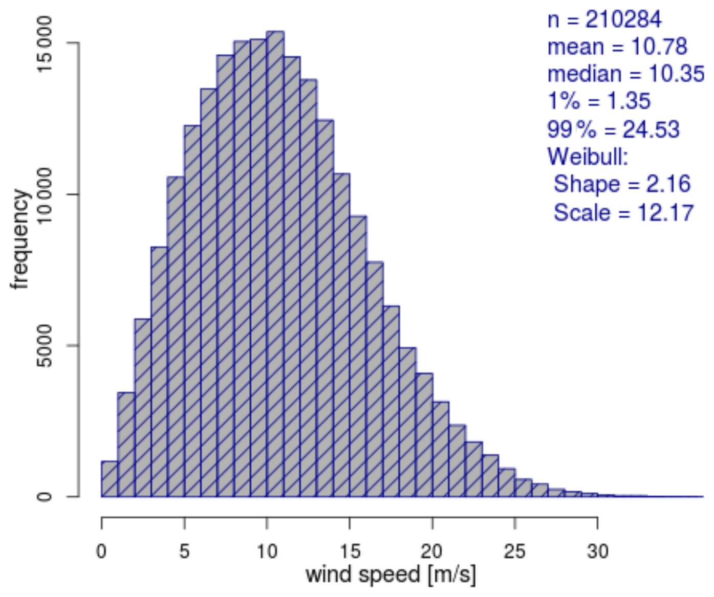
Figure A1 Wind speed histogram with total number of samples (n), mean wind speed, median wind speed, 1 % and 99 % percentiles, and Weibull shape and scale parameters.

Figure A2 Wind direction histogram. Wind speed bins are indicated by different colors.

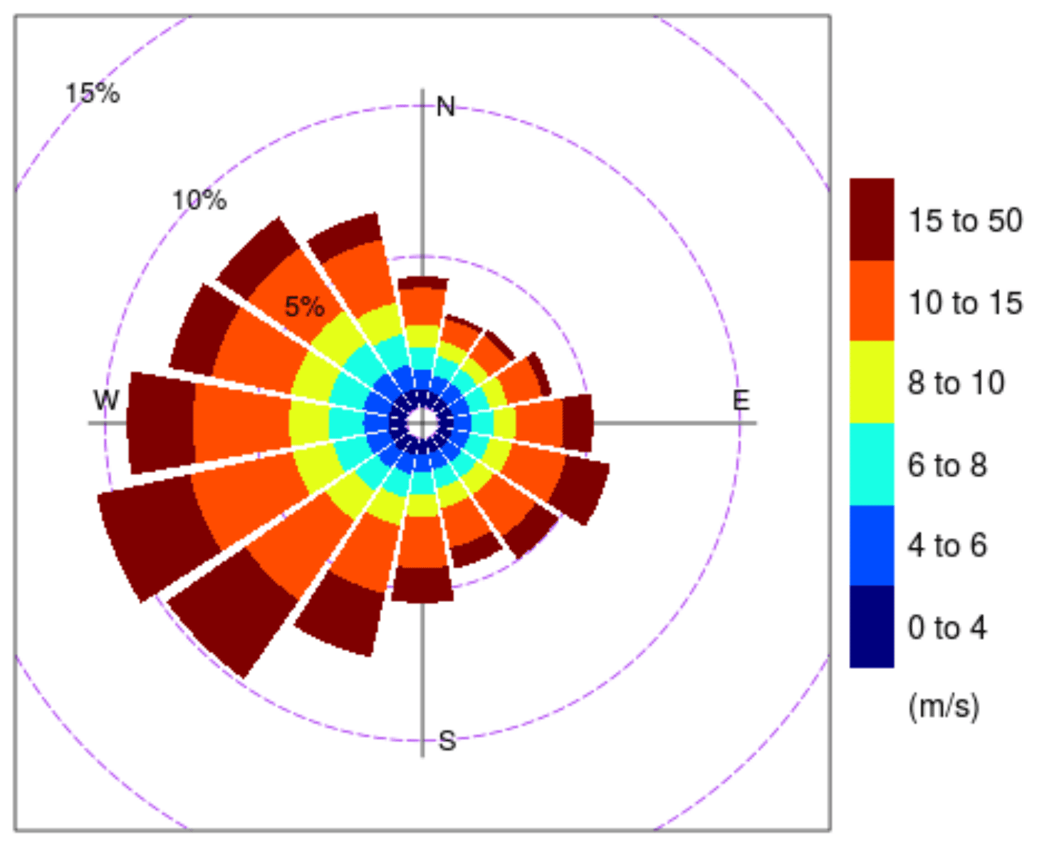
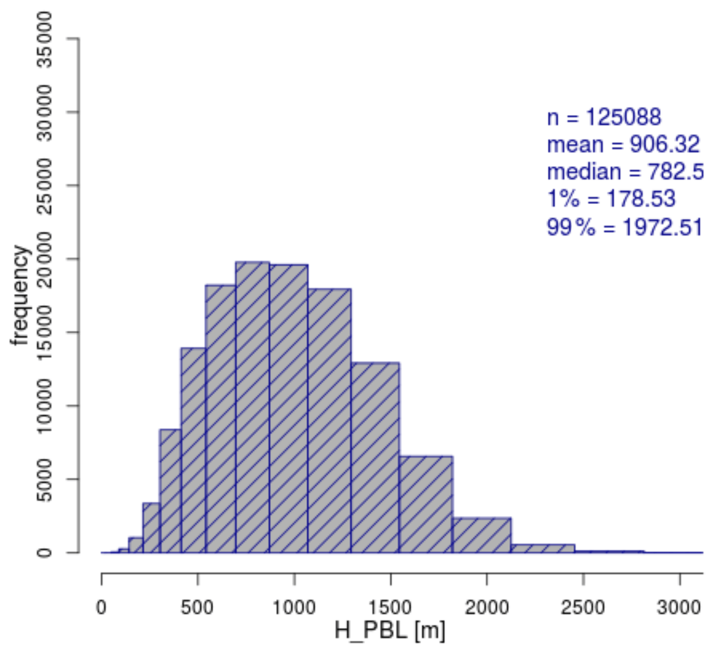
Figure A3 Boundary layer height histogram for convective boundary layers (surface temperature greater than 2 m temperature).

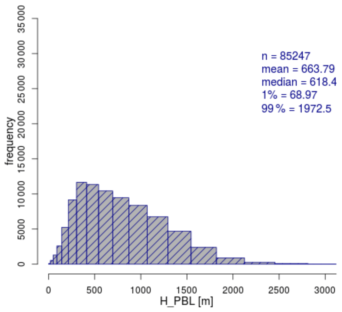
Figure A4 Boundary layer height histogram for stable boundary layers (surface temperature smaller than 2 m temperature).