the Creative Commons Attribution 4.0 License.
the Creative Commons Attribution 4.0 License.
 | 22 Apr 2022
A framework for simultaneous design of wind turbines and cable layout in offshore wind
Nicolaos Antonio Cutululis
An optimization framework for simultaneous design of wind turbines (WTs) and cable layout for a collection system of offshore wind farms (OWFs) is presented in this paper. The typical approach used in both research and practical design is sequential, with an initial annual energy production (AEP) maximization, followed then by the collection system design. The sequential approach is robust and effective. However it fails to exploit the synergies between optimization blocks. Intuitively, one of the strongest trade-offs is between the WTs and cable layout, as they generally compete; i.e. spreading out WTs mitigates wake losses for larger AEP but also results in longer submarine cables in the collection system and higher costs. The proposed optimization framework implements a gradient-free optimization algorithm to smartly move the WTs within the project area subject to minimum distance constraint, while a fast heuristic algorithm is called in every function evaluation in order to calculate a cost estimation of the cable layout. In a final stage, a refined cable layout design is obtained by iteratively solving a mixed integer linear programme (MILP), modelling all typical engineering constraints of this particular problem. A comprehensive performance analysis of the cost estimation from the fast heuristic algorithm with respect to the exact model is carried out. The applicability of the method is illustrated through a large-scale real-world case study. Results shows that (i) the quality of the cable layout estimation is strongly dependent on the separation between WTs, where dense WT layouts present better performance parameters in terms of error, correlation, and computing time, and (ii) the proposed simultaneous design approach provides up to 6 % of improvement on the quality of fully feasible wind farm designs, and broadly, a statistically significant enhancement is ensured in spite of the stochasticity of the optimization algorithm.
- Article
(4150 KB) - Full-text XML
- BibTeX
- EndNote


Offshore wind currently represents one of the main drivers towards power systems fully based on renewable energies. The rapid escalation of this technology has been evident in the last decade (GWEC, 2018), where from 2011 to 2019 the global installed capacity multiplied by a factor of 7, reaching the total of 29 GW worldwide as per the last official consolidated report (GWEC, 2020a). The projected compound annual growth rate of the global offshore wind market is at least 8 % for the starting decade, where yearly new installations are expected to surpass the figure of 20 GW (GWEC, 2020b). In the long term, the target set by the European Commission sees offshore wind providing 450 GW by 2050 (BVG Associates et al., 2019). The previous figures are telling of the development maturity of the offshore wind industry; however certainly the true global expansion has just started.
The massive global proliferation of offshore wind is backed up by the significant developments of wind turbine (WTs) technology, especially in terms of greater nominal power, enlarged production chain capacities, and application of modern installation practices (WindEurope, 2019). In general, projects are today much larger than a few years ago, in the range of 800 MW, with hundreds of WTs rated 6–8 MW (WindEurope, 2020). Apart from the WTs, the set of supporting and auxiliary components of the project (balance of plant, BoP) must be sized as well. This mainly includes submarine cables, offshore transformers, converter stations in case of direct current technology (DC), foundations, structures, and protection/control equipment. WTs alone account today for around 30 % of the overall levellized cost of energy (LCoE), while a similar figure is attributable to the BoP, with submarine cables particularly representing the most expensive component with around 11 % of the LCoE (ORE Catapult, 2020).
As a consequence of economies of scale, the LCoE has considerably decreased in the last decade. However, electrical integration system costs (capital expenses associated primarily with submarine cables and offshore substation) are not following the overall decreasing trend, mainly due to the lack of optimization techniques for designing this subsystem, and the need of longer and bigger submarine cables (Tennet, 2019).
Designing an offshore wind farm (OWF) is a complex and cross-disciplinary scientific task. Given the nature of the technology, a vast number of different disciplines and aspects (or optimization blocks) are involved, theoretically fostering exploitation of the synergies (and trade-offs) between them for the benefit of the system.
Wind farm design optimization is a rich research field that has evolved significantly over the last 2 decades (Ning et al., 2019; Herbert-Acero et al., 2014). Historically, both research and industry methods focused on maximizing the annual energy production (AEP), though more recently the focus has shifted to minimizing the LCoE (or any capital budget evaluation metric) accounting for key cost drivers as well.1 Wind farm optimization addresses the key elements of overall system design and their impacts on the major LCoE elements.
-
AEP. This is driven by the size of the overall turbines (rated power, rotor diameter) and their performance characteristics, as well as their interaction with each other through WT wakes that reduce production from downstream machines. Optimization of the turbine sizing, selection, number, and layout has been considered for the purposes of maximizing AEP. This problem has been studied broadly and intensively. The pioneering work of Mosetti et al. (1994) marked the initial endeavour, applying a genetic algorithm and implementing a similar version of the Katic–Jensen wake decay model (Katic et al., 1986). A plethora of works followed, in general proposing optimization heuristics divided into two categories: (1) gradient-free (heuristics and metaheuristics), such as in Marmidis et al. (2008) (monte carlo), Grady et al. (2005) (genetic algorithm), Wan et al. (2010) (particle swarm optimization), and Wagner et al. (2013) (local search), among others, and (2) gradient-based as in Thomas and Ning (2018), Stanley and Ning (2019a), and Brogna et al. (2020).
-
CAPEX for the BoP. BoP optimization is often done as a sub-optimization problem of the electrical system (a key cost component), though more detailed optimization has also been extensively studied (as will be discussed). Other costs for balance of systems such as the roads for land-based farms and even the installation and logistics strategies have been explored (Roscher et al., 2020).
-
CAPEX for WTs and foundations. While typically the WT itself is taken as fixed, there has been more recent research that even looks at integrated design of the WT and the wind farm (Stanley et al., 2018; Stanley and Ning, 2019a, c; Graf et al., 2016). In addition, for offshore sites with varied sea depths and soil conditions, the design of support structures has been considered either as a sub-optimization or in a sequential optimization (Sanchez Perez-Moreno et al., 2018).
-
OPEX. Reducing OPEX and ensuring site suitability of the WTs for a given layout is a more recent research topic that typically requires using surrogate models to include load models in the optimization (Riva et al., 2020).
While all of these elements are important to full LCoE analysis and optimization of OWFs, one of the strongest trade-offs from an overall cost metric perspective is the placement of WTs and the total length of submarine cables: the more spread out the WTs, the less flow interaction between them – and more AEP, at the expense of larger cable length. Given the theoretical strong dependency and interrelation between them, a coordinated design should bring the best outcome for the whole system.
However, on its own, the design of electrical systems for offshore wind defines a set of highly complex optimization problems. Among them, the cable layout problem for collection systems is defined as how to interconnect the fixed-positioned WTs towards the offshore substations (OSSs), given a set of available cables and engineering constraints (no crossing of cables, maximum number of main feeders, topology, etc.). The cable layout problem maps to standard computer science problems categorized as NP-Hard (Pérez-Rúa and Cutululis, 2019), implying the lack of efficient methods (polynomial running time algorithms), greatly affecting the tractability for large-scale projects. Proposed methods to approach this problem can be categorized as (1) heuristics (Hou et al., 2016a; Pérez-Rúa et al., 2019a), (2) metaheuristics (Hou et al., 2016b; Minguijón et al., 2019), and (3) global optimization (Fischetti and Pisinger, 2018; Pérez-Rúa et al., 2019b), where mixed integer linear programming (MILP) is the most used formulation. A survey and analysis of these methods can be found in Lumbreras and Ramos (2013) and Pérez-Rúa and Cutululis (2019).
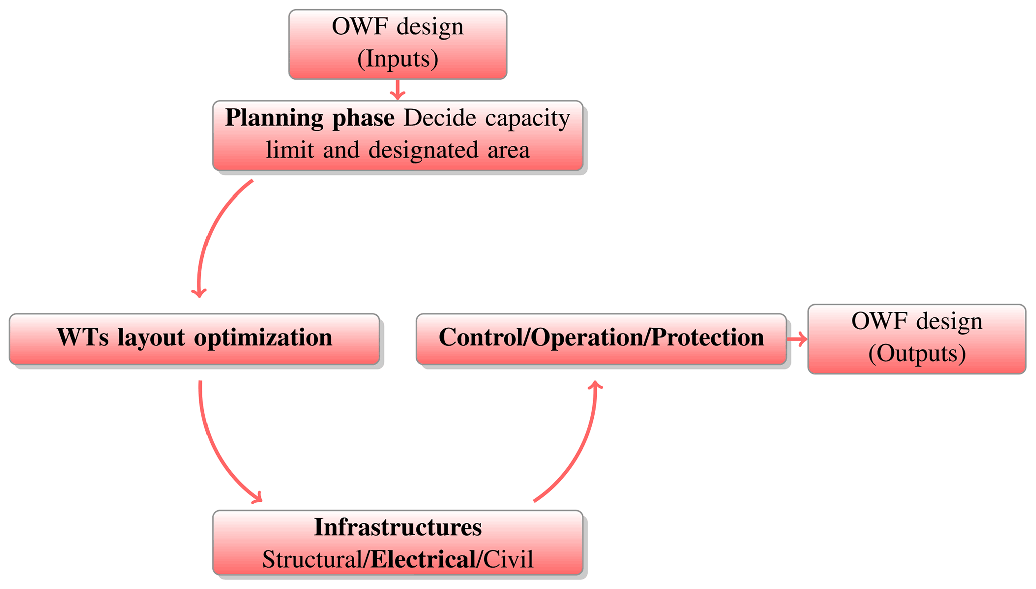
As mentioned before, the a priori strong dependency between WT layout and collection system optimization is a solid motivation to research simultaneous optimization, instead of the classical sequential approach popularly used in the industry (Pérez-Rúa and Cutululis, 2019) (see Fig. 1). The main challenge is developing formulations and methods with good properties: feasibility, numerical tractability, efficiency, effectiveness, and (reduced) complexity for implementation.
A few efforts towards simultaneous optimization of WT layout using gradient-free methods and implementing as cost component heuristic algorithms (incorporated in the objective function or as a constraint) for the cable layout have been identified in previous studies (Sanchez Perez-Moreno et al., 2018; Wade et al., 2019; Amaral and Castro, 2017; Fleming et al., 2016). These algorithms are in general fast, but their calculated cost may differ considerably from the global optimum of the cable layout cost function. Most importantly, feasible designs are not guaranteed using heuristics, therefore still needing a final stage to accurately optimize the cable layout in terms of investment (not addressed in the mentioned literature). Finite grid-based WT layouts have been pre-defined, and the cable layout optimized for each of them using MILP has been optimized in Marge et al. (2019); this procedure allows construction of spatial regression functions to estimate cost functions. However the search space is artificially biased towards a specific topology. A bi-level (nested) multi-objective optimization framework has been proposed in Tao et al. (2021) to address WT layout, cable layout, interaction with the power grid, and power quality, implementing a particle swarm optimization algorithm. Wind turbines and cable layout are solved separately with this metaheuristic algorithm, which potentially would imply a significant problem regarding tractability for large-scale instances. A similar method has been proposed in Wu et al. (2014), where an ant colony system concept is designed and implemented to design the cable layout, relaxing the model by neglecting typical engineering constraints.
In this sense, the main contribution of this article is the proposition of a framework for simultaneous design of WTs and cable layout, where a feasible design is obtained, in contrast to previous works (Sanchez Perez-Moreno et al., 2018; Wade et al., 2019; Fleming et al., 2016). This framework is benchmarked against the sequential approach commonly employed in the industry. The comparison is elaborated in terms of feasible design using high-level economic metrics. Aiming to study the underlying operating principles of the proposed framework, a systematic investigation of the performance of the heuristic for cable layout optimization is performed, having as reference the exact optimization model for the cable layout design (Pérez-Rúa et al., 2019b). Likewise, a sensitivity analysis for different OSS positions is presented, in order to quantify the effect over the performance comparison.
2.1 Engineering wind farm model, AEP calculation, and WT layout design
The engineering wind farm model implemented in this paper is the so-called IEA-37 Simple Bastankhah Gaussian available in PyWake (Pedersen et al., 2019). This model is composed of (i) a component to propagate the wake in the wind farm, performing a minimum of deficit calculations, by studying the effect of a particular WT over its downstream WTs. This procedure neglects upstream blockage effects but is computationally fast. The model also includes (ii) a component to compute the previously mentioned wake velocity deficits between pairs of WTs and (iii) a component to superpose the deficits for turbines placed in multiple wakes to obtain the total velocity deficit through a squared sum operation. Formulae of this model are available in IEA Wind Task 37 (2019).
Let X and Y be a set of abscissas and ordinates respectively of the nw WTs to install for the OWF to be optimized. The AEP for this particular layout is calculated taking into consideration the WT parameters (most importantly the power curve), the number of wind directional bins (fixed to 16 in this paper), and the site's wind rose. A valid layout represented by X and Y must satisfy two basic constraints: (i) WTs must be placed inside of the polygon that defines the OWF designated area, and (ii) a minimum distance of 2D between WTs, where D is the WT diameter, must be guaranteed.
2.2 Collection system cable layout
The aim is to design the cable layout of the collection system for an OWF, i.e. to interconnect the nw WTs to the available OSSs, no, using a list T of cables available, minimizing the total investment cost. The collection system cable layout optimization is represented as a static problem with respect to time, with the nominal power being generated by the WTs. This is to ensure robustness on the design given the uncertainty associated with real-time power profiles. For simplicity, only one OSS is considered; hence no=1. Let the WTs define the sets, and . The physical locations of points in N are correspondingly available in S as abscissas (x1 for OSS and X for Nw) and ordinates (y1 for OSS and Y for Nw) in the two-dimensional space. The Euclidean distance between the positions of the points i∈N and j∈N is denoted as dij. The complete weighted directed graph gathers all relevant graph-related parameters, where N represents the vertex set, A the set of arcs arranged as a pair set , and D the set of distances da.
Regarding cables, let the capacity of a cable t∈T be ut measured in terms of number of WTs connected downstream. Hence, let U be the set of capacities sorted as in T. Each cable type t has a cost per unit of length, ct∈C, in such a way that T, U, and C are all comonotonic.
Generally, a feasible collection system design includes the following engineering constraints.
- [C1]
-
A tree topology must be enforced. This means that there must be only one electrical path from each WT towards the OSS.
- [C2]
-
The capacity of cables must not be exceeded.
- [C3]
-
The number of main feeders, i.e. cables directly reaching the OSS, must be limited to a maximum ϕ.
- [C4]
-
Cables must not lay over each other (no crossing cables) due to practical installation aspects.
As explained in the introduction, the formally elucidated problem above can be tackled with methods classified into three groups: heuristics, metaheuristics, and global optimization. Section 2.2.1 focuses on a specific class of heuristics (two-steps), and Sect. 2.2.2 concentrates on an exact model based on a MILP formulation which brings along an optimality certificate. This allows assessment of how far away the best known solution is to the best known achievable objective value computed as a percentage gap. Both methods are applied in the proposed optimization framework. Metaheuristics are excluded from this work as their value is usually utilized when stand-alone solver-free robust methods are required for the cable layout optimization problem. It is considered a cumbersome endeavour to harmonize metaheuristic methods for both the cable and WT layout problem in either a nested or fully integrated fashion.
2.2.1 Heuristics optimization algorithms
Heuristics are defined in this application as solver-free polynomial running time algorithms, which, through a set of sequential steps, construct a (hopefully) feasible design or infeasible point with an associated cost. In either case, heuristics are useful in this context for obtaining a very fast estimation of the cost of the cable layout for given WTs and OSS position. This is required since during the iterative process of simultaneously solving the WTs and cable layout problem, function evaluations are repeatedly executed to compute the value of the high-level economic metric as part of the process to move throughout the search space. The faster the heuristics, the more iterations for a given computing time budget and thus the more exhaustive the design exploration.
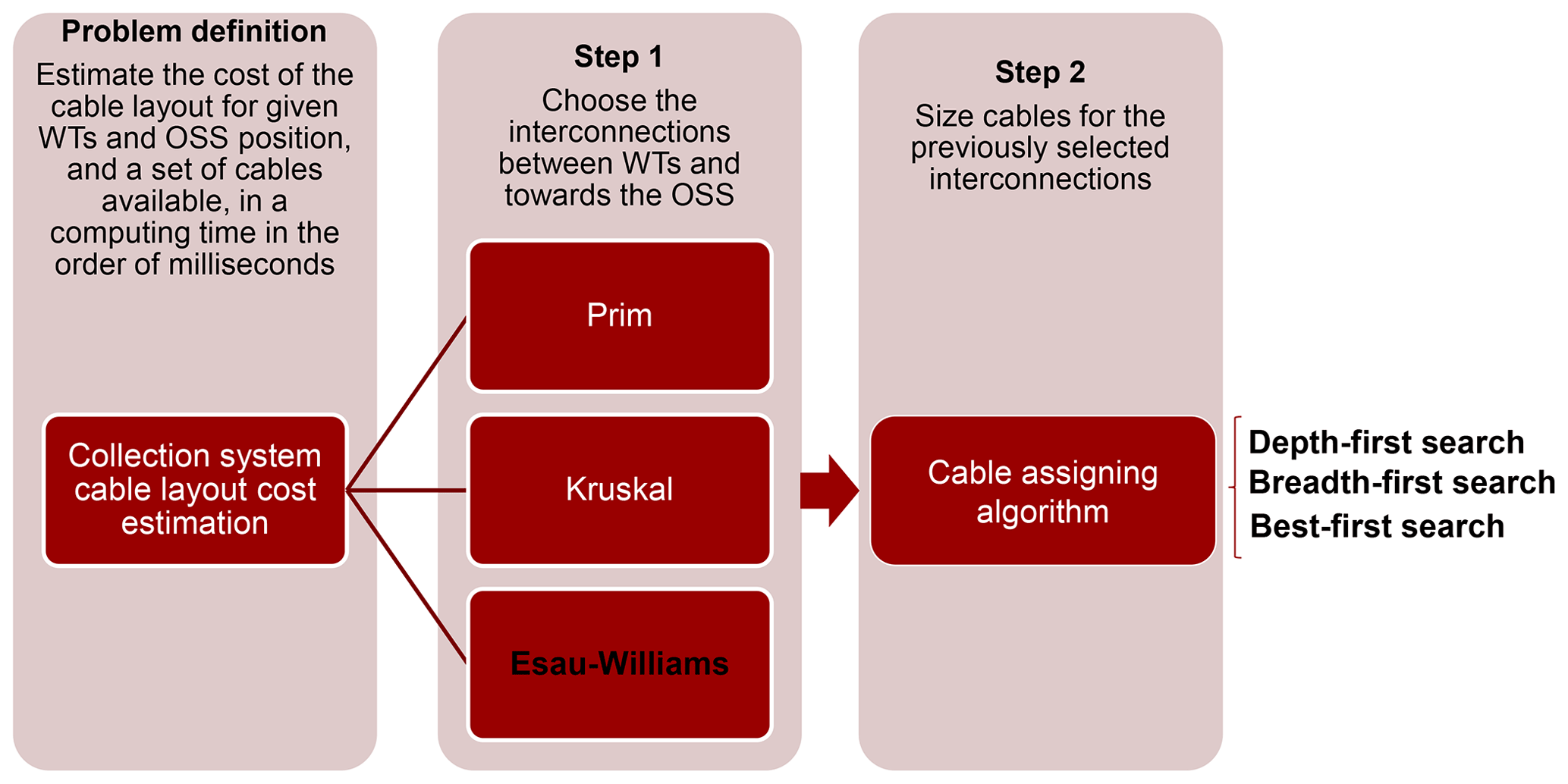
The flowchart of the heuristic implemented in this article is presented in Fig. 2. The algorithm consists of a two-step decision process, where the first step selects the arcs that connect WTs to each other and towards the OSS. As illustrated in Fig. 2, several capacitated minimum spanning tree (C-MST) greedy heuristic algorithms can cope with the first step, such as the Prim, Kruskal, Vogel, and Esau–Williams algorithms, among others. Although these algorithms have been proposed individually (Prim, 1957; Kruskal, 1956; Chandy and Russell, 1972; Esau and Williams, 1966), they intrinsically follow the same underlying rules during the design construction process (Kershenbaum, 1974; Kershenbaum and Chou, 1974), based on the generalization of trade-off cost functions updated correspondingly for each case.
The satisfiability of [C1], [C2], [C3], and [C4] is sought in Step 1. [C1] is fulfilled by means of avoiding the interconnection of elements in N belonging to different components at a given iteration, with subsequent updating of disjoint component sets after merging them if all other constraints are not violated. [C2] is guaranteed through the limitation of node number to of any maximal subgraph connected to the OSS with a single arc. [C3] is enforced by simply controlling the number of arcs reaching the OSS. Finally, [C4] is respected by checking at a given iteration the candidate arc with the cumulative set of selected arcs.
[C1] is deemed a fundamental constraint, considering that the problem is closely defined to generate trees, and any other topology would lead to a very unrealistic cost compared to the global minimum. Computational experiments carried out in a previous work (Pérez-Rúa et al., 2019a) showed that the coexistence of [C2] with [C3] (and by extension [C4]) frequently leads to infeasible points (i.e. a forest graph), as a result of backtracking inability. This means that one needs to prioritize the exclusive evaluation of these constraints. The relaxation of [C2] could harden the calculation of the cable layout cost estimation, considering that the cost vector C is bounded to the available set of cables T. Consequently, the reasoning to disregard [C3] and [C4] is twofold. First, the computational aspects related to the evaluation of these constraints are avoided, reducing the computing time for every function evaluation. Second, as the nature of these heuristics overestimates the cost of the cable layout (due to the two-step process), the relaxation of [C3] and [C4] could help decrease the gap with respect to the global minimum.
Ultimately, the Esau–Williams algorithm has consistently performed better in terms of feasible points and investment cost quality, when framed in the method of Fig. 2, than the other greedy heuristics (Pérez-Rúa et al., 2019a). On that account, a modified version of the Esau–Williams heuristic is solely implemented in this work. The pseudocode for Step 1 is presented in Algorithm 1.
The input of the algorithm is collected in the weighted directed graph. The first five lines initialize the useful sets. The most important is the trade-off set To using the weight parameters pi; note that due to the weight parameter definition, an arc and its inverse must be considered independently. The iteration process starts at line six and continues until a fully connected tree graph is obtained. In each iteration the arc with the lowest trade-off value is incorporated in the tree, as long as it satisfies [C1] and [C2] (lines seven to nine). According to the trade-off value, priority is given to the arcs located the farthest to the OSS for the same arc length, as the greater the pi, the lower the ta. In case constraints are met, the component sets (that include nodes i and j of the selected arc ao) are merged, and the trade-off values linked to the newly formed component are updated (lines 10 to 14). Otherwise, the arc ao and its inverse become completely banned from the design process, by equalizing their trade-off values to infinity (lines 16 to 17). The indirect graph Gd in line 19 contains the graph tree nullifying any directionality of arcs.
In Step 2, any algorithm for traversing or searching Gd can be applied with the purpose of determining the number of WTs connected downstream in each edge e∈Eo. Efficient algorithms are, for instance, depth-first search (Tarjan, 1972), breadth-first search (Zhou and Hansen, 2006), and best-first search (Dechter and Pearl, 1985).
Let β be the number of WTs connected through edge e∈Eo with length de. The following trivial optimization problem must be solved: , with being the -tuple binary set. The solution provides the cheapest cable t∈T able to support β WTs via binary variable , where each tuple defines an independent problem solved in linear running time.
Algorithm 1Step 1 of Fig. 2
2.2.2 Global optimization: MILP model
When a problem is formulated within the framework of a MILP paradigm, state-of-the-art solvers can be applied in search of high-quality solutions with a proven optimality certificate. MILP models are generally more efficient than mixed integer quadratic programming (MIQP) and mixed integer non-linear programming (MINLP); therefore they are the preferred choice for the nature of this problem. A challenge is then how to incorporate real-world engineering aspects into the optimization, such as quadratic power losses or other types of non-linearities. In the following, a basic model, stemming from Pérez-Rúa et al. (2019b), with the goal to design the cable layout to minimize total investment, while satisfying [C1] to [C4], is deployed.
Equation (2) defines the variables of the model. Binary variable xij is 1 if the arc (i,j) is selected in the solution and zero otherwise. Likewise, binary variable models the k number of WTs supported upstream (with respect to flow towards the OSS) from j, including the WT at node j (under the condition that xij=1). Function f(i), which allows for variable number reduction, maps from tail node i to the maximum number of WTs connectable km through an arc (i,j). If i=1 (i.e. the OSS), then , otherwise .
Equation (3) is the objective function. Cost parameter encodes the optimum cost to connect k WTs through arc (i,j) and is obtained similarly to Step 2 in Fig. 2. [C2] is enforced at this point as well. Equation (4) simultaneously ensures a tree topology, only one cable type used per arc, and the head (j)-tail (i) convention, while Eq. (5) is the flow conservation which avoids a forest graph; both Eqs. (4) and (5) guarantee [C1]. Equation (6) expresses the requirement of [C3]. The set χ stores pairs of arcs , which cross each other. Excluding crossing arcs ([C4]) in the solution is ensured by the simultaneous application of Eqs. (7) and (8). Finally, Eq. (9) defines a set of valid inequalities to tighten the mathematical model.
The MILP model from Eqs. (2) to (9) presents fewer variables and constraints than flow-based formulations (Pérez-Rúa et al., 2019b). The latter, in practical terms, facilitates the convergence of solvers in the matter of computing time and memory. Nevertheless, computational limitations are still conspicuous when solely applying the full model using state-of-the-art solvers, as for instance the branch-and-cut by CPLEX (IBM, 2021). As a way around this difficulty, an algorithmic framework wraps up the MILP model as a way around this difficulty, as shown in Fig. 3.
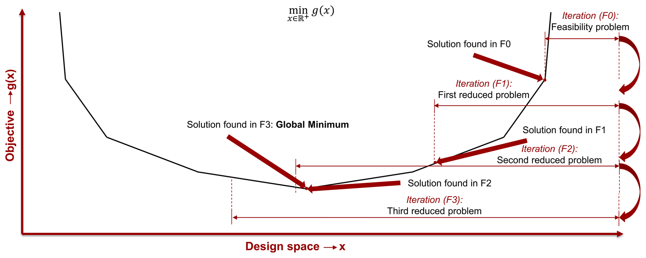
The algorithmic framework of Fig. 3 consists of a progressive enlargement of the design (search) space from a rather small size (feasibility problem F0) to a larger one (iteration F3) to (hopefully) reach the global minimum. The transition between iterations is given by a step size determined heuristically and defined as the number of candidate arcs from a WT towards neighbouring ones; this implies that in each iteration, model Eqs. (2) to (9) are reformulated, such as . Each iteration is warm-started with the incumbent solution for the sake of shortening the processing, resembling a hill-climbing approach. A compromise between computing time and likelihood to cover the global minimum must be accounted for within this optimization model. The stopping criterion is finding the same solution in two consecutive iterations, indicating that further enlarging the design space is not required, as represented between F2 and F3 in Fig. 3.
2.3 Optimization framework
The objective is to design an OWF that will maximize the internal rate of return (IRR) of the project. The IRR estimates the profitability of potential investments using a percentage value rather than a dollar amount (Investopedia, 2021), making it preferable by investors in many situations. IRR is often in agreement with other capital budget evaluation metrics as a net present value (NPV). The higher the value of IRR, the better a project from the investor's perspective, as it can cover higher values of weighted average cost of capital (WACC). The implemented IRR model (DTU Wind Energy, 2021) is comprehensive and takes into account a wide range of costs, like DEVEX (costs spent in the period from idea to development to design and planning), CAPEX (expenditures in the period of construction up to the date the OWF is commissioned), OPEX (costs in the operational period), and ABEX (costs related to abandonment of the OWF) (Megavind, 2021).
The AEP directly affects the cash flow along the project lifetime, while the collection system cable layout cost is reflected uniquely in the CAPEX. Therefore, IRR could implicitly favour AEP (annual cash flow) over cable layout cost (CAPEX). The comparison between AEP and cable costs may then be conservative within this framework and would challenge to a greater extent the benefits of a simultaneous design of these aspects. As per the results of Sanchez Perez-Moreno et al. (2018), the strongest trade-off is determined between the cables and the WT layout, which is further studied in this paper. Trade-offs between WT foundations and WT structures are deemed negligible for sites with a uniform seabed profile and topographically homogeneous available area.
The function to estimate the cost per metre for each element in C is presented in Eq. (10) (Lundberg, 2003). The cost function is scaled to take into consideration macroeconomic phenomena such as inflation and exchange rate.
where , , and are coefficients dependent on the nominal voltage of cable type t∈T, is the rated power of t in VA (also depending on the rated line to line voltage level, Vn), and ct is the cost of t in euros per kilometre. Note the exponential cost trend in function of the rated power.
2.3.1 Design approaches
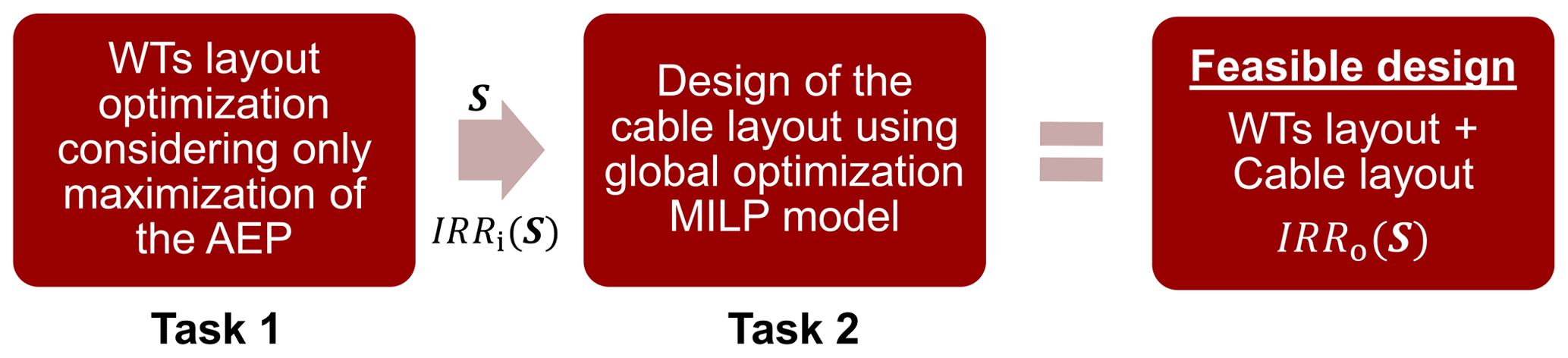
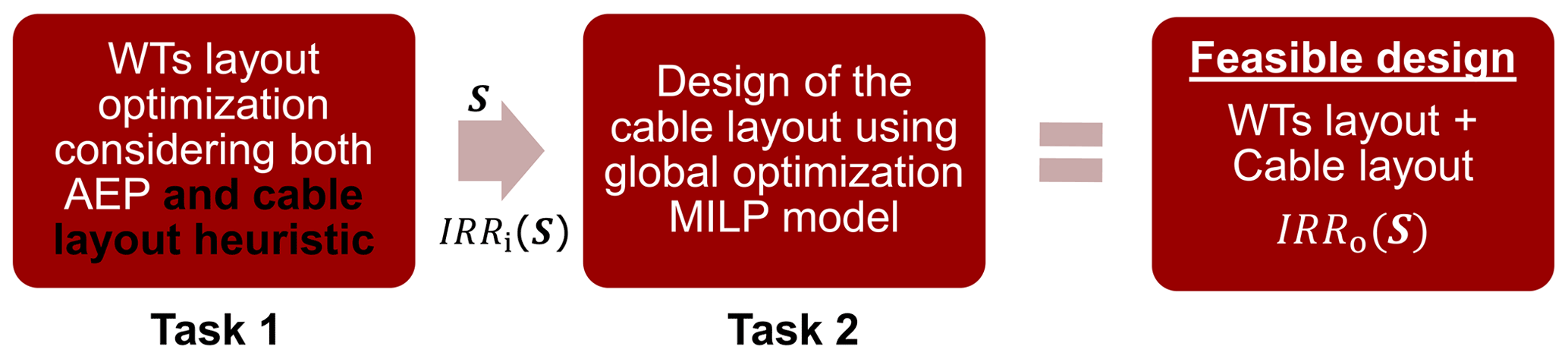
The classical sequential approach is presented in Fig. 4, where the WTs and cable layout optimization are completely decoupled. The simultaneous approach presented in this paper is shown in Fig. 5, incorporating an initial cable layout optimization (Fig. 2) in Task 1. For both approaches, Task 2 defines the final cable layout (based on the method of Sect. 2.2.2) given the position of WTs and OSS decided in Task 1, S. In the end, a feasible design is obtained for both cases, respecting all constraints of Sect. 2.1 and 2.2, with an associated objective function value for each.
2.3.2 Optimization algorithm: random search
The optimization algorithm for Task 1 of Fig. 4 (sequential, Approach 1) and Fig. 5 (simultaneous, Approach 2) is deployed in Fig. 6. The random search algorithm was first proposed by Feng and Shen (2015) as a tailor-made method for the WT layout problem using a gradient-free technique. This algorithm has been designed to maximize the AEP and according to computational experiments outperforms other gradient-based and gradient-free algorithms for OWFs with 20 to 80 WTs (Feng and Shen, 2015; Brogna et al., 2020). While for Task 1 of Fig. 4 gradient-based algorithms can be implemented, in the case of a simultaneous design of WTs and cable layout, the intrinsic discontinuous non-smooth nature of the cable layout cost function extremely hardens the computation of analytical or numerical derivatives. As a result of this condition, gradient-free, tree search, or local search solvers emerge as good alternatives to tackle a simultaneous design (Hutter et al., 2011).
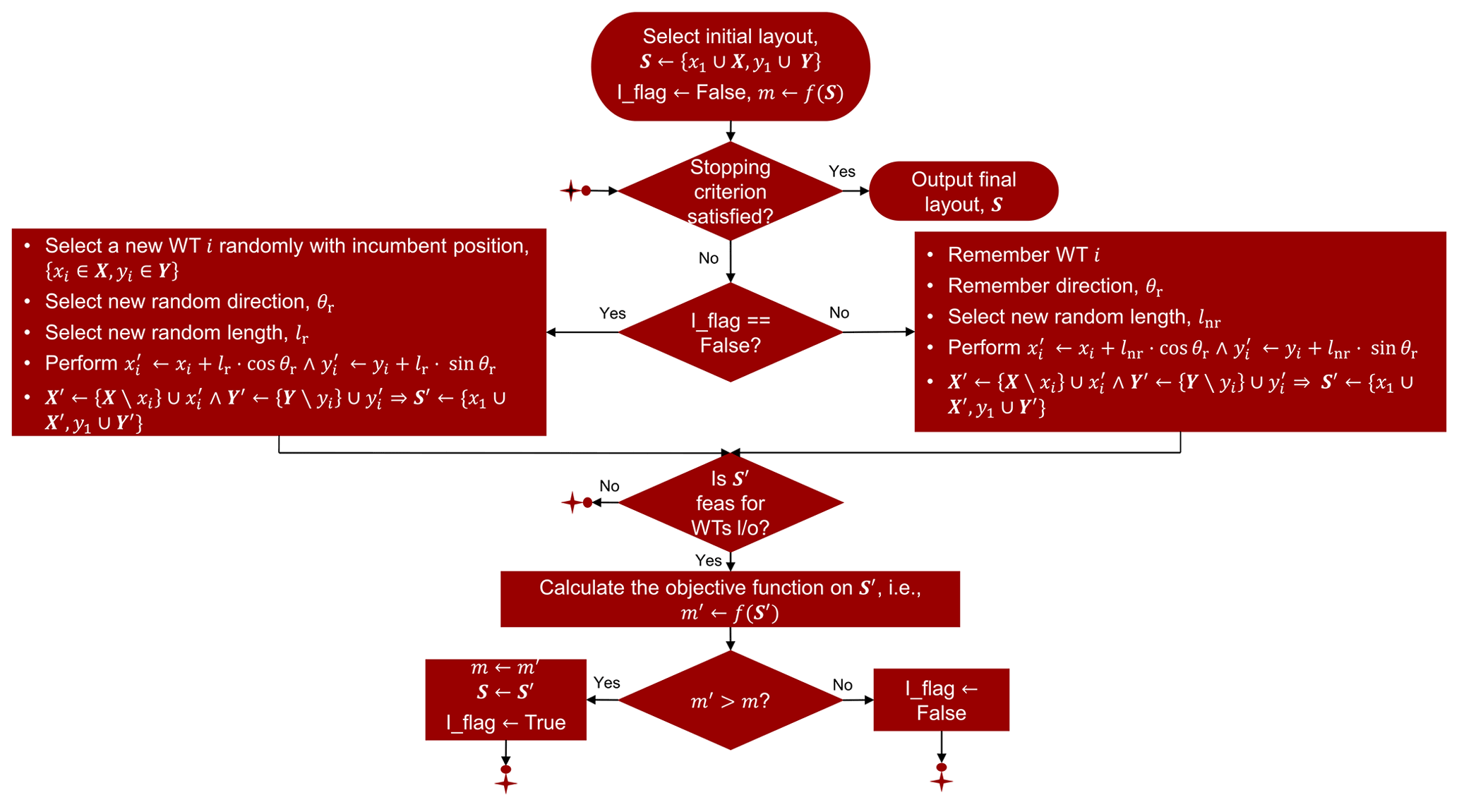
A generalization of the random search algorithm for generic objective function is diagrammed in Fig. 6. The coordinates set, S; the improvement flag, I_flag; and the incumbent value of the objective function m=f(S) (in this case as mentioned before, IRRi(S)) are initialized. When applied in Approach 1, m assumes a zero cost for the cable layout during the whole iterative process of computing IRRi(). In contrast, when implemented in Approach 2, m considers both the cash flow from the AEP and capital cost from the cable layout as estimated by the process of Fig. 2, for a given S.
Through the output of Task 2 in Figs. 4 and 5, the overall IRR, IRRo(S), in each case is computed accounting for the global minimum cost of the cable layout, a value that is used in the final comparison analysis.
Since, in theory, the location of the OSS, {x1,y1}, can take infinite values, a course of action is to fix the OSS location in the centroid of the WTs. However, only considering the project area centroid could lead to unrealistic designs, as presented in Fig. 7, where an overlapping between a WT and the OSS appears. In order to decrease the occurrence likelihood of this erratic design, a simple heuristic rule for the OSS location is presented in Fig. 7. The OSS is displaced to the centroid of the four nearest WTs, in case the original distance between the points denoted by the OSS and nearest WT is under a specific threshold. For the particular case of a square disposition of WTs, assuming a minimum distance between WTs of 2D, a minimum distance between OSS and WT of is ensured after this correction. This heuristic does not guarantee success in respecting the distance threshold for any WT arrangement; however, it represents a good compromise between effectiveness and computing burden.
Continuing with the flowchart of Fig. 6, after checking out the stopping criterion (computing time tr in this paper), the process carries on with either moving a random WT i across a random direction θr and length lr or continuing with picking up the same WT i as in the previous iteration, moving it towards the same direction θr with new random length lnr. A WT i is shifted towards the same direction θr, if improvement of the objective function has previously been gained in a feasible design in terms of the WT layout (constraints presented in Sect. 2.1). Otherwise a new WT prospect is evaluated as stated before. Note that the layout initially generated evolves during the running of the algorithm, where the incumbent layout S, objective function m, and current WT prospect i with direction θr are memorized and eventually used for learning purposes in subsequent iterations. This algorithm follows a hill-climbing path with stochasticity incorporated.
The simplicity and rather low computational burden of the algorithm are very important bright sides that ultimately play a major role in its favour concerning tractability and effectiveness, as gradient-free algorithms typically call a great number of function evaluations (Stanley and Ning, 2019b). These properties are notoriously important for large-scale problems (nw>70).
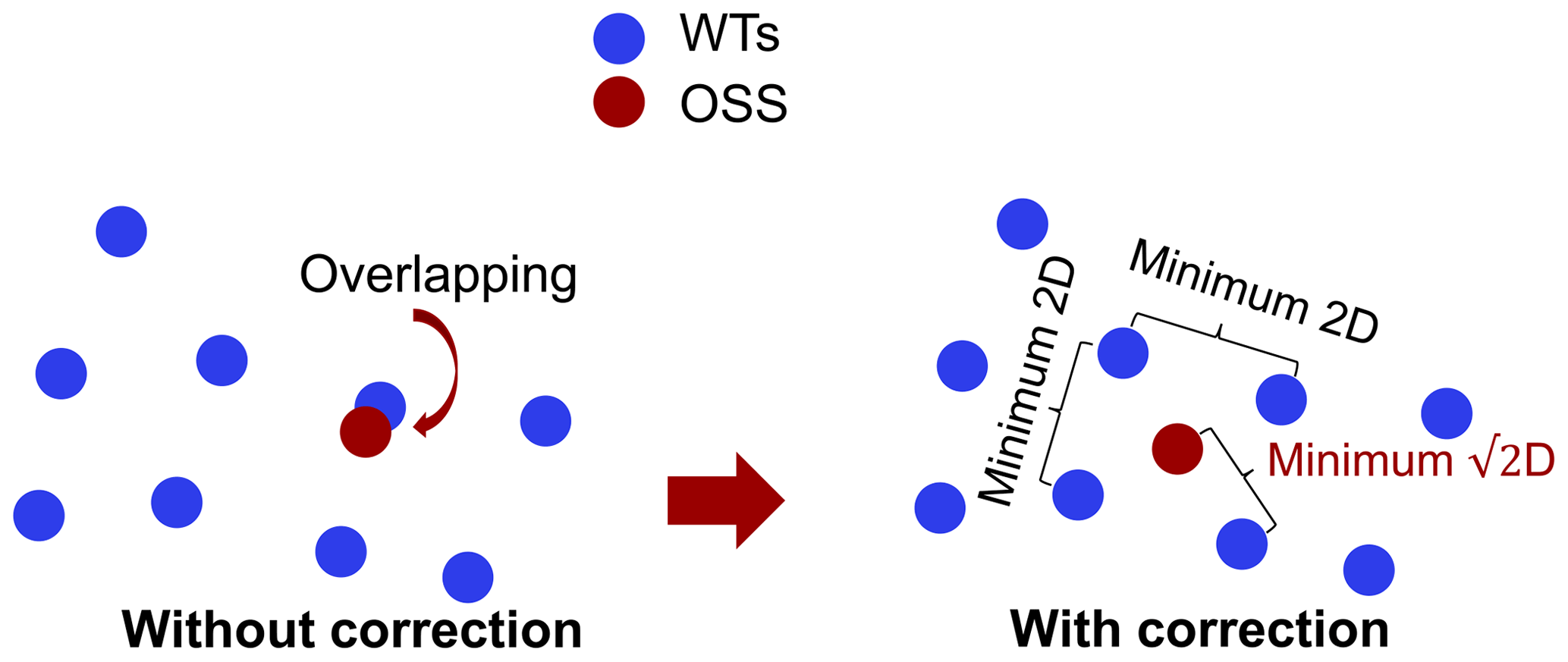
Figure 7Simple heuristic for relocation of the OSS at approximately the centroid of the WTs.
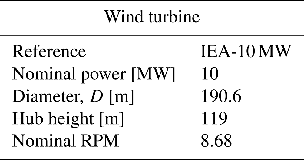
The methodology presented in Sect. 2 is applied to the reference OWF IEA-37 Borssele (Dykes et al., 2015), with the OWF designated area defined as the convex hull of the polygon vertices. The project consists of 74, 10 MW each, IEA Task 37 reference WTs (Bortolotti et al., 2019). The main input parameters for the OWF and WT are presented in Tables 1 and 2 respectively. The short distance to shore (10 km) permits focus on the collection system cable layout rather than in the export system (Pérez-Rúa et al., 2020). In turn, a uniform seabed profile sheds lights on the synergies between WTs and cable layout, as foundations and structures then have an unique design. The energy price of EUR 27 EUR per MWh corresponds to the minimum median of the hourly spot prices in the Nordic–Baltic–central western European (CWE) power markets so far in 2021 (Nord Pool, 2021).
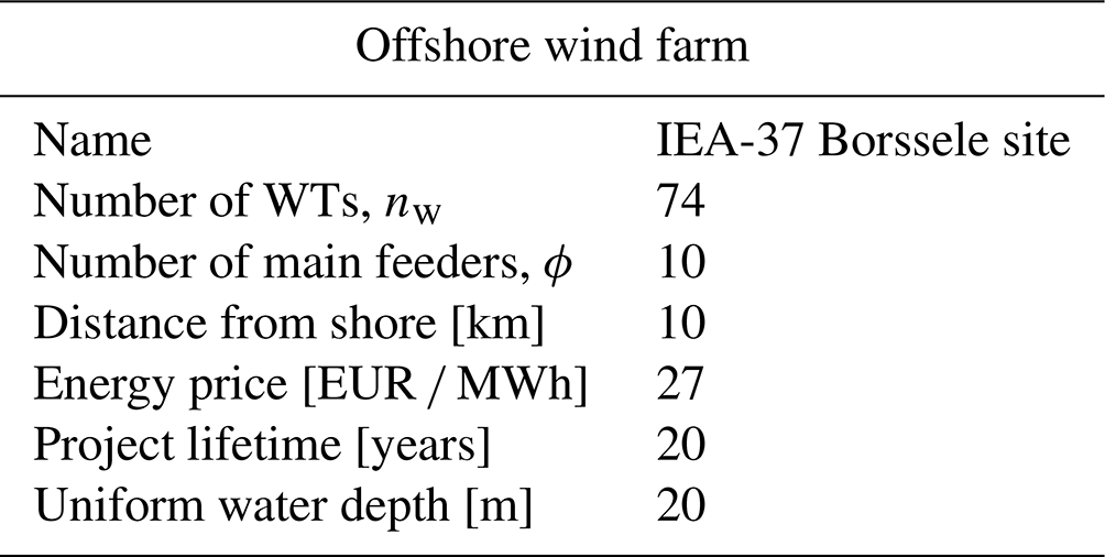
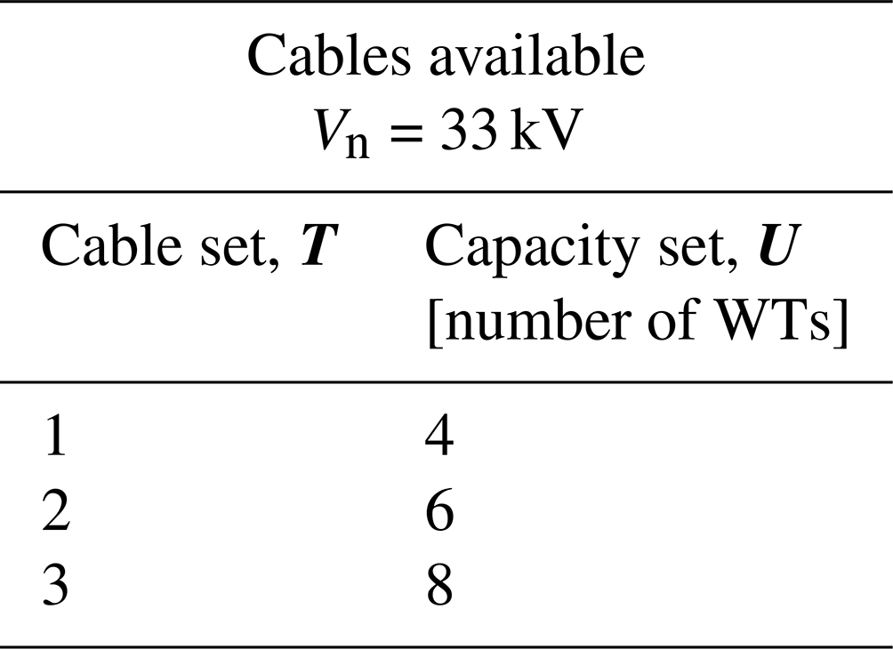
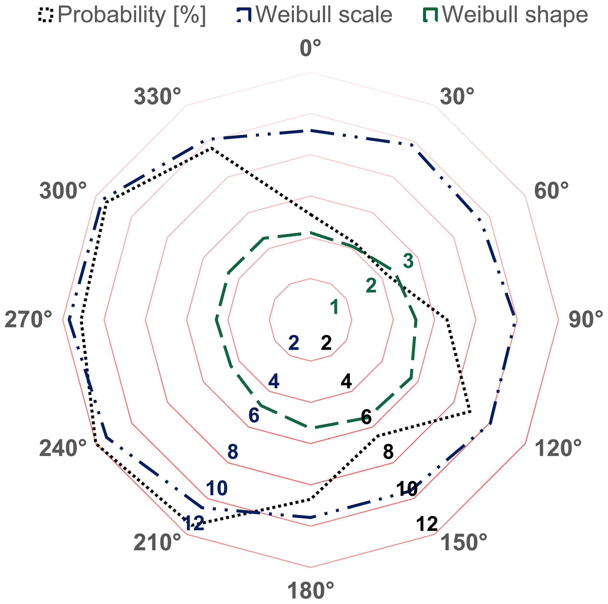
Table 2 deploys the data related to the set of cables available, rated at a voltage level of Vn=33 kV, and their thermal capacity as defined in Sect. 2.2; by means of the set U and Vn, the cost set C is calculated implementing Eq. (10). Finally, the site's wind rose in Fig. 8 shows that the prevailing winds come in the sector from 210 to 300∘ in the Cartesian reference plane.
The experiments have been carried out on an Intel Core i7-6600U CPU running at 2.50 GHz and with 16 GB of RAM. Workflows for Task 1 in Figs. 4 and 5 have been implemented in the TOPFARM framework (DTU Wind Energy, 2018). The chosen MILP solver for Task 2 is the branch-and-cut solver implemented in IBM ILOG CPLEX Optimization Studio V12.10 (IBM, 2021).
3.1 Performance analysis of the cable layout algorithms
One of the main hypotheses for the effectiveness of Approach 2 (Fig. 5) is the accuracy of the estimation of the cable layout cost by the heuristic of Fig. 2. The closer this cost estimation is to the global optimization model (Sect. 2.2.2), the better the results of the simultaneous WT and cable layout design.
Aiming at performing a systematic evaluation of the heuristic algorithm, a pool of WT layouts were generated through the implementation of Approaches 1 and 2, by varying the computing time tr of the random search algorithm from a few seconds up to 48 h (≈210 000 function evaluations). Two different location criteria of the OSS are simulated for both approaches; first, at approximately the centroid of the WTs with possible correction as presented in Fig. 7, and second, at a designated location outside the OWF area.
It is important to bear in mind that the purpose of this section is not to draw conclusions about the difference in the objective function value of both approaches, but to focus on the difference of costs obtained from the heuristic and the global optimization model for the cable layout associated with each of the generated WT layouts. Intuitively, by utilizing Approach 1, a larger distance between the WTs would be expected, maximizing the AEP, but the opposite is expected with Approach 2, as the cost of cables is taken into consideration. The stochasticity of the random search algorithm is advantageous for having a pool of realistic WT layouts with high diversity within the previously described behaviour.
The performance analyses of the cable layout algorithms are graphed in Figs. 9 and 10. For each WT layout from the generated pool, the average and standard deviation lengths between pairs of WTs are computed (in rotor diameters, D); both measures provide a quantitative indication of how spread out the WTs are from each other within the OWF designated area: the greater the average and deviation length, the more separated and scattered they are. In blue are displayed the results corresponding to WT layouts generated after Approach 2, and in red the ones after Approach 1 are shown. Triangle and circles are for OSS at approximately the centroid and at external location respectively.
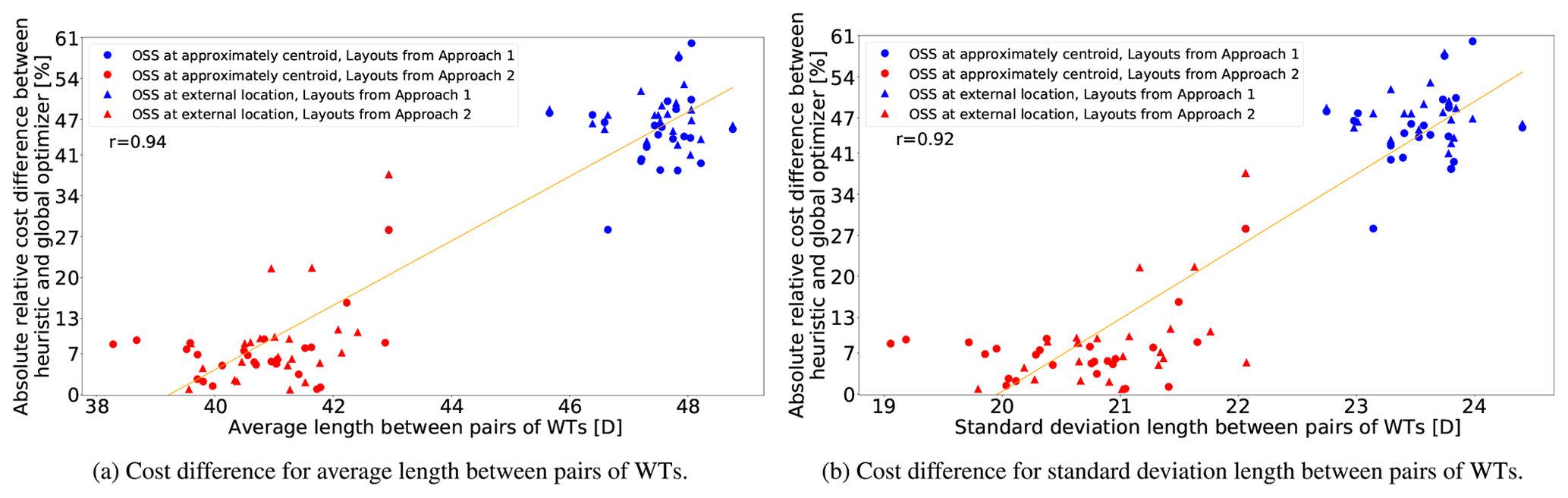
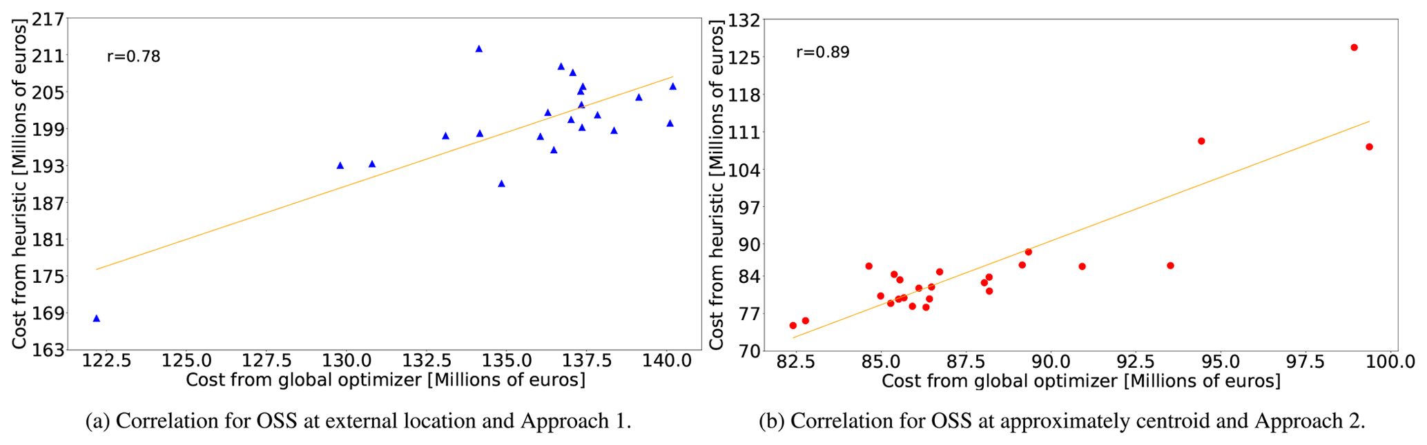
Figure 9a shows the absolute relative cost difference between methods with respect to the global optimization model vs. average length, and Fig. 9b shows the global optimization model vs. standard deviation length. This figure confirms the initial expectation regarding the placement of WTs in each approach; there are clearly two clusters of points, for average length greater than 45 D and standard deviation length greater than 22.7 D, the layouts from Approach 1 are placed, while for Approach 2 this is the case for values less than 43 D and 22.1 D respectively. Points at average 43 D and standard deviation 22.1 D correspond to tr≈0 (computing time of the random search algorithm; see Fig. 6), i.e. the initial layout which is in the centre of the scale approximately. This outcome reflects the effect of including the cable layout over the WT layout optimization process. It is also interesting to note that the clustering is independent of the OSS location. The second takeaway is the strong correlation between cost difference vs. average length (Pearson coefficient, r=0.94) and cost difference vs. standard deviation length (r=0.92). This means that the heuristic algorithm performs better at estimating for dense WT layouts. The average absolute relative cost differences are 46 % and 8 % for Approaches 1 and 2 respectively. This is a remarkably large difference in function of WT layout characteristic.
From another perspective, Fig. 10 displays the correlation between the costs from the heuristic and the global optimization models. Figure 10b evidences the good but not so strong correlation for those layouts associated with Approach 2. In Fig. 10a the correlation is even worse for data obtained from Approach 1. According to these results, the heuristic algorithm leads to worse results in terms of cost difference and cost correlation for less dense WT layouts. An ideal heuristic would have a cost difference of 0 %, correlation of 1, and very fast computing time (order of a few hundred milliseconds). The latter is confirmed, as for all presented results the heuristic takes between 100 ms and 300 ms, while the exact method can go up to 10 h for gaps lower than 2 %. More computing time (on average an order difference of hours to minutes) of the global optimization model is experienced for dense WT layouts than for spread ones.
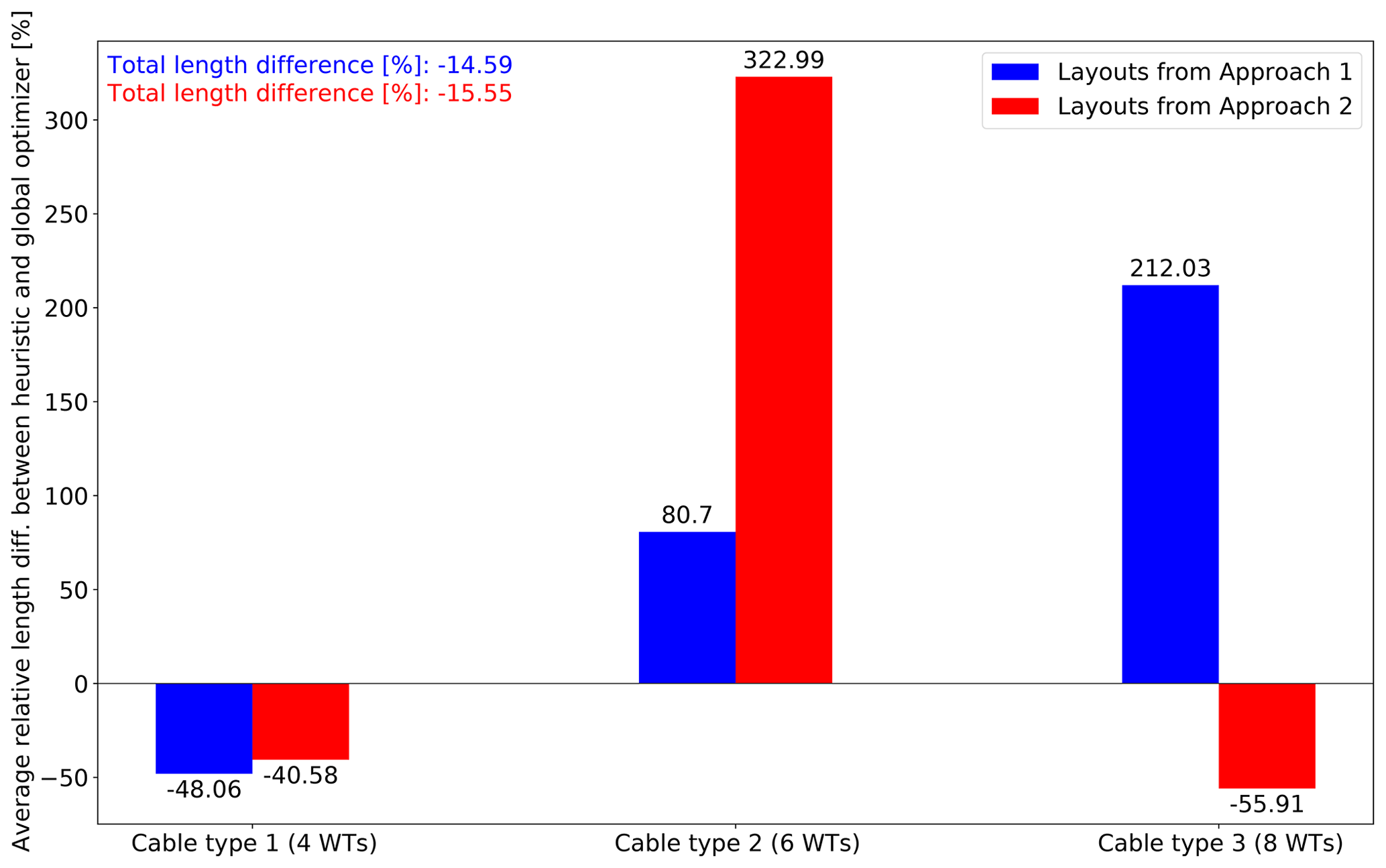
Figure 11Cable length comparison between cable layout algorithms for OSS at approximately the centroid.
The previous results suggest a compelling aspect: the initial layout impacts the overall optimization process, as the initial cost estimation from the heuristic would likely be inaccurate. The more spread in the initial layout, the greater the penalization of the cable layout cost during the first iterations. The degree of impact of this deviation is yet unclear and hard to predict, but a seemingly good hypothesis is that a detriment of the final solution could be caused due to a potential sizeable reduction of the AEP. The absolute relative cost difference and correlation linked to the initial layout, and to the layouts towards denser arrangements, are deemed good enough for this application.
To understand the underlying reason for the performance observed in Figs. 9 and in 10, the usage of available cables of Table 3 by Approach 1 and Approach 2 (with OSS at approximately the centroid) is shown in Fig. 11, where the average relative length differences with respect to the global optimization model are plotted for each cable type and approach. It can be noted that the heuristic designs cable layouts in Approach 1 using a disproportionately large amount of the most expensive cable (212 % of type 3), even though the designed total length of cables is shorter with 14.59 % on average. This trend is also noticeable for cable type 2 with an excess of 80.7 %. The cheapest cable (type 1), on the contrary, is used less by the heuristic. The exponential cost nature of cables (Eq. 10) causes this length disparity to be reflected even more sharply monetarily. Notwithstanding this issue, for Approach 2 the most pronounced difference is shifted to cable type 2, but with the other two cables used less. The results for layouts from Approach 2 point out that a better balance of cable usage allows for a smaller cost difference and stronger correlation between both cable layout design methods. This evidence can be understood due to the trade-off function of Algorithm 1, which causes bigger clusters of WTs to be formed when they are widely spread out, leading to main feeders to support more WTs. More dense WT layouts result in smaller groups of WTs and consequently more main feeders. This suggests that a WT-layout-dependent trade-off cost function could bring along benefits for the performance of the heuristic algorithm.
3.2 Statistical analysis between Approach 1 and Approach 2
After a sensitivity analysis, the computing time for the statistical study between both approaches is fixed to 36 h (≈170 000 function evaluations), a value regarded to be statistically sufficient to leverage the frameworks of Figs. 4 and 5 based on numerous computational experiments. Due to the rather high computational time, eight runs of the method in Fig. 6 are executed for Approaches 1 and 2 with both possible OSS locations.
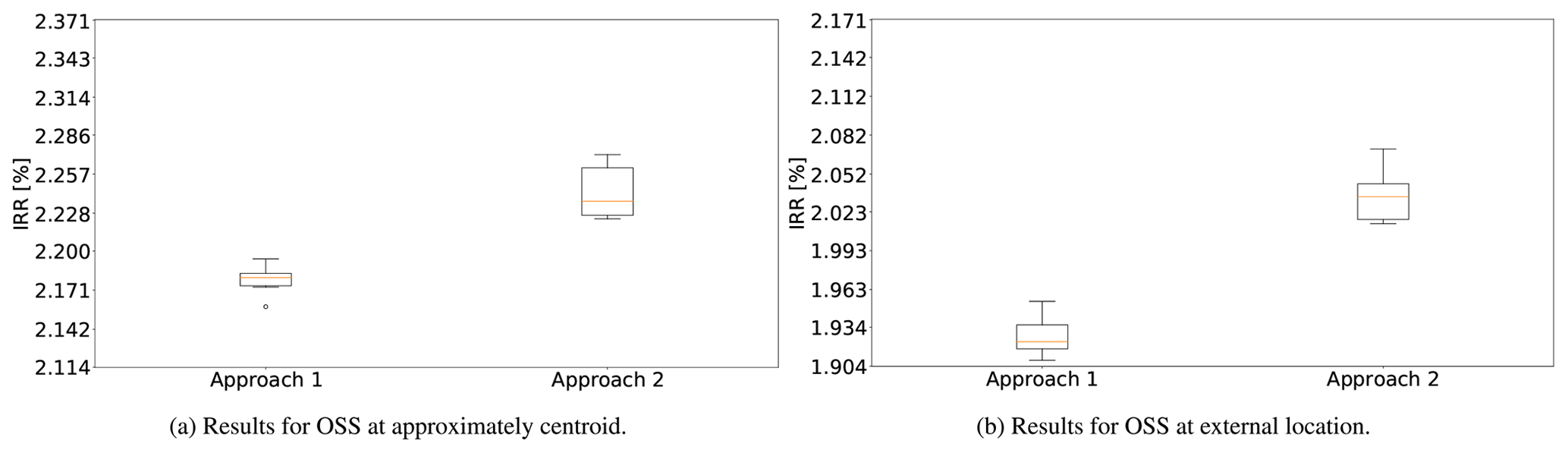
The graphical representation of IRR for the four cases (approaches × OSS locations) through box-and-whisker diagrams with an inclusive median is displayed in Fig. 12. For the centroid OSS, all realizations from Approach 2 result in a better IRR (Fig. 12a) than Approach 1, with an improvement between maximum values of 3.52 %. Less dispersion in the data linked to Approach 1 is noticed, with standard deviation of 0.011 % vs. a standard deviation of 0.020 % in Approach 2. An interpretation to this effect is that the heuristic introduces a high variability in function of the WT layout. The benefits from the simultaneous approach are visible in Fig. 12b, with an IRR improvement between maximum values growing to 6 % for the external OSS, also presenting a larger variability than the data from the sequential approach (0.020 % vs. 0.015 %). The larger improvement in the case of an externally located OSS is attributed to the higher cost of the cable layout (see Fig. 10), increasing the weight of this cost share in the overall economic metric (IRR). Approach 2 is hence able to exploit situations where submarine cables are extensively required, for example with different OSS locations, number of WTs, rated power, designated area, etc.
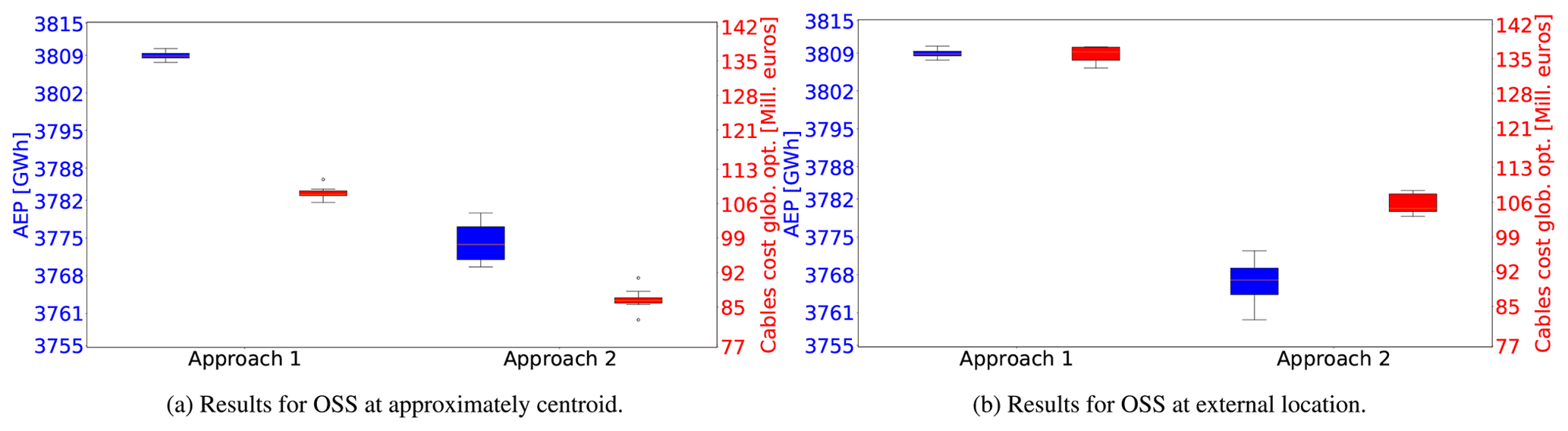
The observed differences of IRR between approaches presented in Fig. 12 are broken down in terms of AEP of cable layout cost in Fig. 13. Approach 1 consistently provides WT layouts with greater AEP than Approach 2 in both OSS locations, at the expense of more costly collection system networks; this illustrates the (most likely nonlinear) correlation between AEP and cable layout cost. The robustness of the AEP maximization process when neglecting the cable layout (Approach 1) is evidenced by the rather low standard deviation (0.79 MW, approximately 0.02 % of the average value). The previously elucidated variability of IRR in Approach 2 (Fig. 12) is also reflected in the AEP spread, which has a standard deviation of roughly 0.1 % of the average value for both OSS locations. Oppositely, the spread of the cable layout cost is not as marked as for the AEP, yet a larger variation between Approaches 1 and 2 is still observable.
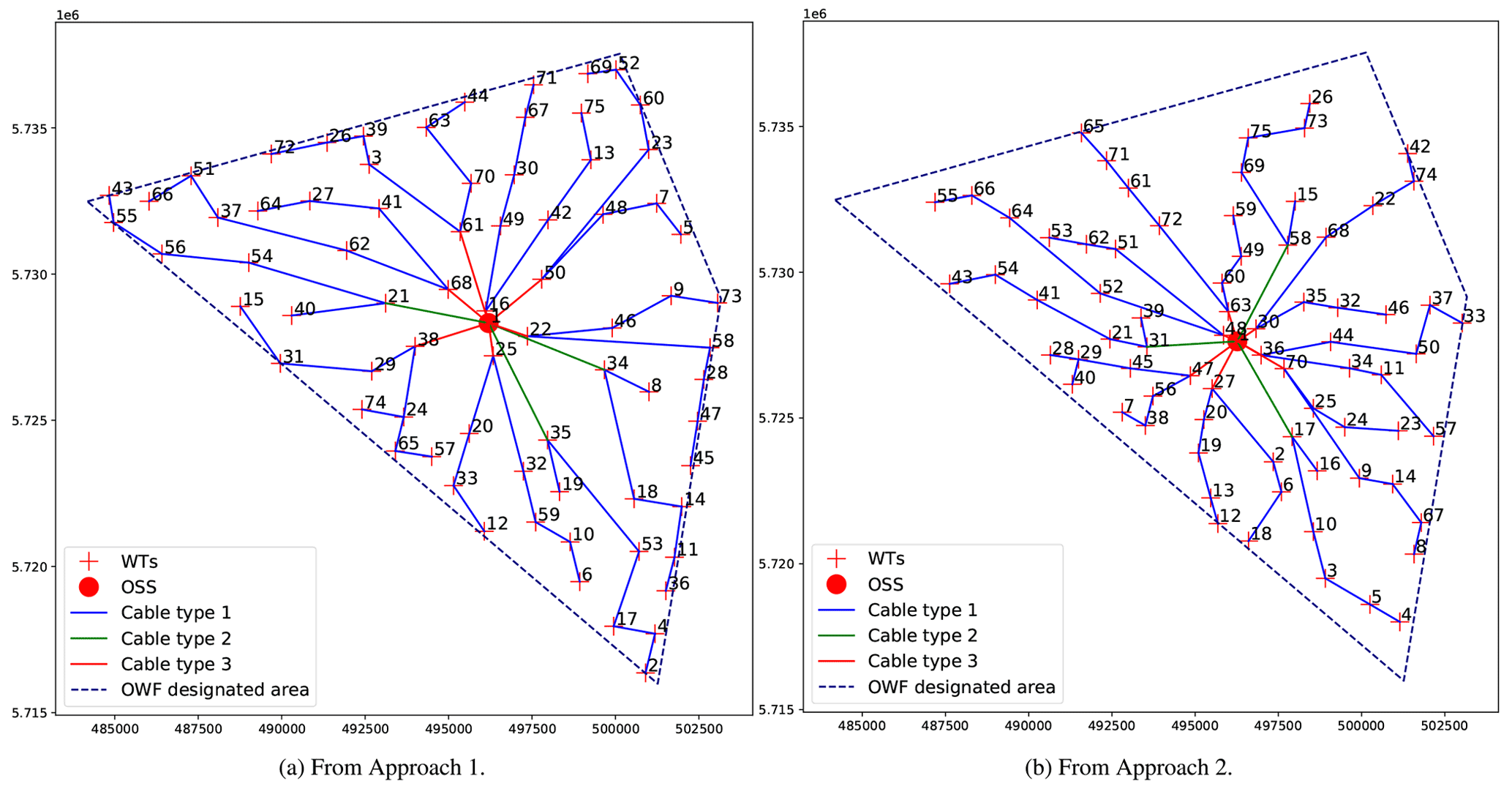
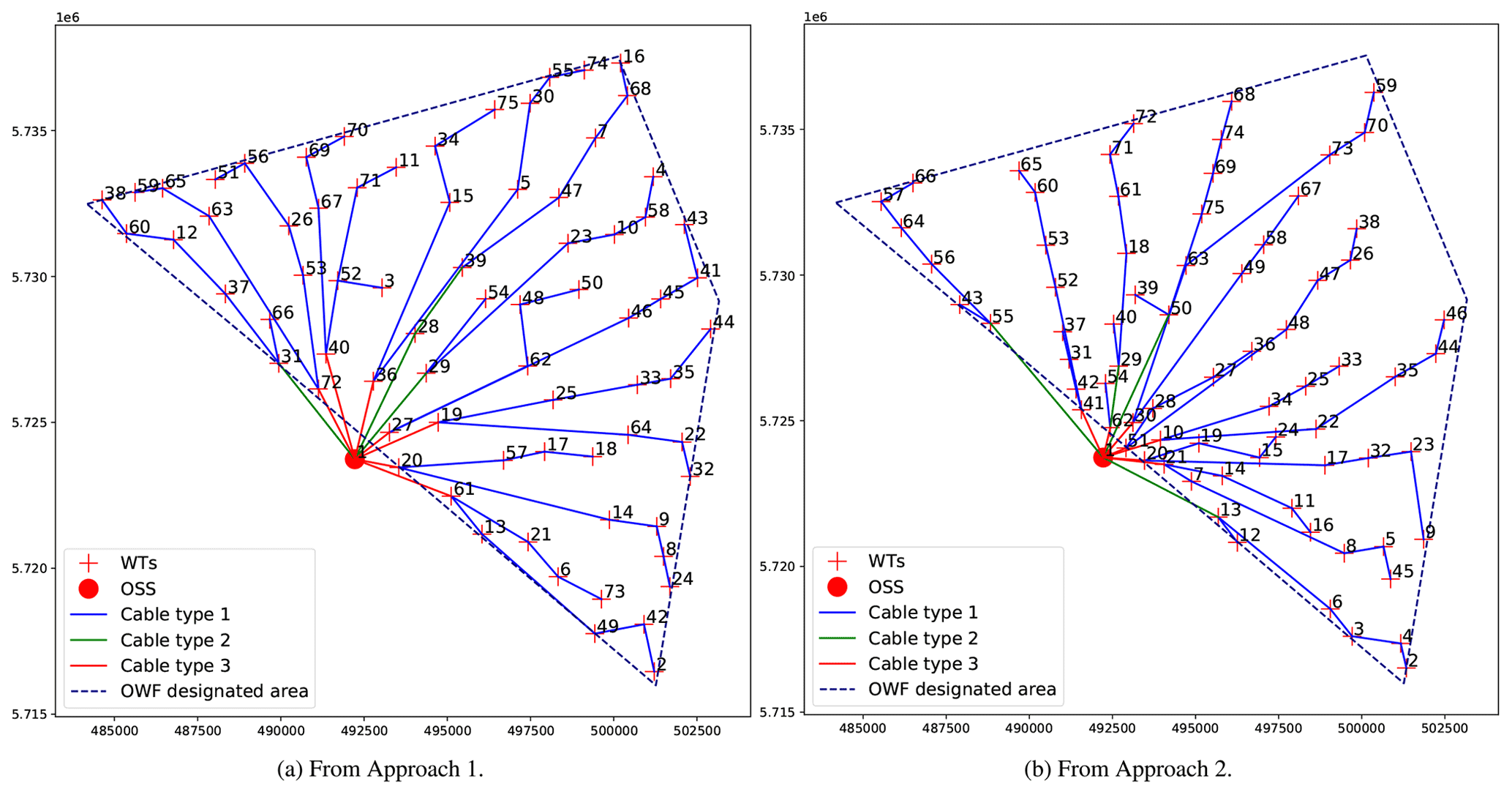
The best layouts obtained by each approach – for centroid and external OSS respectively – are shown in Figs. 14 and 15. It is evident that the main difference between the pairs of OWFs is the concentration of WTs within the OWF designated area. Note how both layouts from Approach 1 utilize the area more, with WTs highly concentrated at the OWF borders, in contrast to those from Approach 2 where the WTs are closer to each other. The impact of the site's wind rose (Fig. 8) is also clear, as WTs are mostly aligned towards the prevailing wind direction (third quadrant of the coordinate plane).
Beyond the improvement over the overall IRR in random finite realizations, the contribution of the simultaneous approach should also be assessed from a statistical perspective to prove a significant impact, considering the stochasticity of the optimization algorithm. A t test for independent samples is conducted with this in mind. The main assumption to validly perform this parametric test is that the populations linked to each sample set are normally distributed. Although the probability distributions of both approaches are unknown and inaccessible, the normal distribution is a good default choice in this case of absence of prior knowledge about the form of the function (Goodfellow et al., 2016). Two reasons which back up this supposition are, first, the central limit theorem and, second, the fact that a normal distribution encodes the maximum amount of uncertainty over the real numbers.
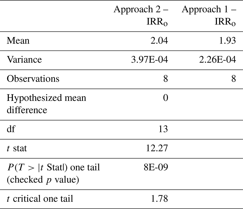
Tables 4 and 5 summarize the results of the t test assuming unequal variances for centroid and external OSS at approximately the centroid and externally located respectively. The null hypothesis is that the mean difference between feasible designs obtained from both approaches is equal to zero; i.e. Approach 2 does not improve Approach 1. Results are very clear: for both cases, the p value is almost 0 % (focus on the results of a one-tail distribution given that the directionality of average comparison is clearly defined), meaning that there is a statistically significant difference between the two approaches, with the simultaneous one providing on average feasible designs located in a subset of the objective function's domain with greater quality than those stemmed from the sequential approach.
The results suggest two points. First, that the objective function defined in Task 1 of Fig. 5, IRRi(), succeeds at having a good representation of the target function IRRo(), due to the good performance of the heuristic for cable layout design. An average absolute relative difference between IRRi and IRRo for several runs of Fig. 5 equal to 2.4 % and 3.89 % for OSS at centroid and outside respectively compared to the results of Fig. 4 of 50.69 % and 70.41 %, correspondingly, proves this aspect. Second, the ability of the simultaneous optimization framework to consistently find points which belong to a region of the target objective function with higher quality than the sequential counterpart is shown.
Table 4The t-test-independent two-sample distribution assuming unequal variances for OSS at approximately the centroid.
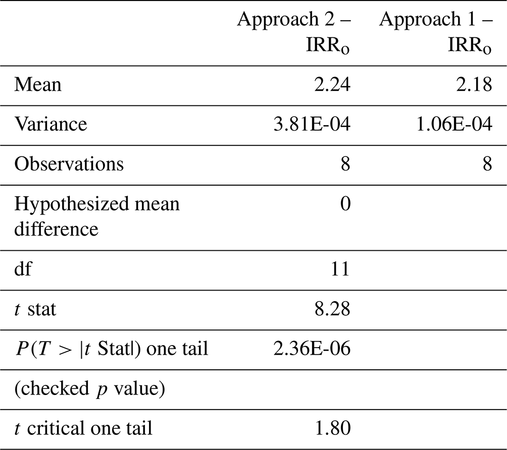
Table 5The t-test-independent two-sample distribution assuming unequal variances for OSS at an external location.
The presented results are project-dependent and therefore are vulnerable to variations in the set of input parameters. An increase in energy price would result in a heavier weighting of AEP during the optimization process, giving priority to a more spread-out WT layout. The cable costs are another important parameter, which in turn if they were greater could more strongly favour the cable layout design by bringing together the WTs; similar logic applies for OSS location further away from the WTs. The available area is also deemed key, since larger areas would give more room to exploit trade-offs between WT and cable layouts when applying Approach 2.
The proposed method provides an approach for simultaneous design of WTs and cable layout. The approach supports typical engineering constraints frequently used in this context, including OWF designated area, minimum distance between WTs, tree topology for cable layout, thermal limits of available cables, maximum number of main feeders, and no crossing of cables.
The main novelties of this paper are (i) proposition of the simultaneous optimization framework, harmonizing different algorithms (random search, heuristic for the cable layout, and global optimization model) and resulting in a formulation and method with good computational properties, such as tractability, efficiency, and effectiveness. (ii) Systematic performance assessment of the fast cost estimation from the cable heuristic compared to the global optimization model, identifying a connection between WT layouts and quality (relative difference, correlation, and computing time) of the estimation, which is considered fundamental for the full framework success is shown. (iii) Rigorous benchmark of the proposed method vs. the current practice using statistical tools is shown.
The proposed simultaneous methodology has been applied to a large-scale offshore wind farm, demonstrating its feasibility and superiority compared to the sequential counterpart (Approach 1). The heuristic algorithm for the cable layout performs reasonably well for layout arrangements with higher density, with an average absolute relative cost difference with respect to the global optimization model of 8 %. The heuristic informs the random search algorithm of this cost share during the iterative simultaneous optimization process. A sensitivity analysis for two different OSS locations (at approximately the centroid and external of the OWF) points out the high correlation between the benefits of the simultaneous approach (Approach 2) and the overall weight of the cable cost. For the OSS located at approximately the centroid, an improvement of the IRR of 3.52 % is achieved, while for the external OSS, the improvement is boosted to 6 %.
Finally, based on multiple runs of the optimization algorithm, it is possible to conclude that feasible points obtained after Approach 2 are located on average in a region of the objective function's domain with higher quality than those from Approach 1. This proves the effectiveness of the framework defined by Approach 2 in representing the complete objective function well, supporting both the WTs and cable layout (IRR), by means of the heuristic as a surrogate model, and at the same time, the capacity to obtain feasible points belonging to that domain region.
Typical values for the input parameters (energy price, cable costs, available area, and OSS location, among others) are utilized to set up the case study. However, the outperforming capacity of Approach 2 over Approach 1 is affected by variations in those conditions: more expensive energy prices can result in a better performance of a sequential design approach, while greater cable costs could have the opposite effect. A more detailed analysis of the impact of those parameters on the results of the optimization could constitute future work.
Code is available at https://doi.org/10.5281/zenodo.6470472 (Pérez-Rúa et al., 2022a).
Data generated from this research are available at https://doi.org/10.5281/zenodo.5913079 (Pérez-Rúa et al., 2022b).
JAPR designed the algorithms, approaches, and case studies with inputs from NAC. JAPR implemented the model and carried out the numerical experiments. JAPR and NAC analysed the results. JAPR prepared the manuscript with contributions from NAC.
The contact author has declared that neither they nor their co-authors have any competing interests.
Publisher’s note: Copernicus Publications remains neutral with regard to jurisdictional claims in published maps and institutional affiliations.
The authors thank Katherine Dykes for her support in setting up TOPFARM simulations, general discussions, and feedback on the manuscript and Mathias Stolpe for the discussions and inputs shaping the case studies.
This research has been supported by the Danmarks Frie Forskningsfond, DFF (grant no. 1127-00188B), under the project “Integrated Design of Offshore Wind Power Plants”.
This paper was edited by Michael Muskulus and reviewed by Michael Muskulus.
Amaral, L. and Castro, R.: Offshore wind farm layout optimization regarding wake effects and electrical losses, Eng. Appl. Artif. Intel., 60, 26–34, https://doi.org/10.1016/j.engappai.2017.01.010, 2017. a
Bortolotti, P., Tarrés, H. C., Dykes, K., Merz, K., Sethuraman, L., Verelst, D., and Zahle, F.: IEA Wind Task 37 on Systems Engineering in Wind Energy, WP2.1 Reference Wind Turbines, https://doi.org/10.2172/1529216, 2019. a
Brogna, R., Feng, J., Sørensen, J. N., Shen, W. Z., and Porté-Agel, F.: A new wake model and comparison of eight algorithms for layout optimization of wind farms in complex terrain, Appl. Eng., 259, 114189, https://doi.org/10.1016/j.apenergy.2019.114189, 2020. a, b
BVG Associates, Recognis, and WindEurope: Our Energy Our Future, Tech. rep., BVG Associates, edited by: Colin Walsh, WindEurope, https://windeurope.org/wp-content/uploads/files/about-wind/reports/WindEurope-Our-Energy-Our-Future.pdf (last access: 22 April 2022), 2019. a
Chandy, K. M. and Russell, R. A.: The Design or Multipoint Linkages in a Teleprocessing Tree Network, IEEE T. Comput., C-21, 1062–1066, https://doi.org/10.1109/T-C.1972.223452, 1972. a
Dechter, R. and Pearl, J.: Generalized best-first search strategies and the optimality of A*, J. ACM, 32, 505–536, https://doi.org/10.1145/3828.3830, 1985. a
DTU Wind Energy: TOPFARM, https://topfarm.pages.windenergy.dtu.dk/TopFarm2/index.html# (last access: 19 April 2022), 2018. a
DTU Wind Energy: DTU Cost Model, https://topfarm.pages.windenergy.dtu.dk/TopFarm2/api_reference/dtucost.html (last access: 19 April 2022), 2021. a
Dykes, K., Rethore, P., Zahle, F., and Merz, K.: IEA Wind Task 37 Final Proposal. Wind Energy Systems Engineering: Integrated RD&D, Tech. rep., International Energy Agency, 2015. a
Dykes, K., Hand, M., Stehly, T., Veers, P., Robinson, M., Lantz, E., and Tusing, R.: Enabling the SMART Wind Power Plant of the Future Through Science-Based Innovation, Tech. Rep. TP-5000-6812, NREL, https://doi.org/10.2172/1378902, 2017. a
Esau, L. R. and Williams, K. C.: On teleprocessing system design, Part II: A method for approximating the optimal network, IBM Syst. J., 5, 142–147, https://doi.org/10.1147/sj.53.0142, 1966. a
Feng, J. and Shen, W. Z.: Solving the wind farm layout optimization problem using random search algorithm, Renew. Energ., 78, 182–192, https://doi.org/10.1016/j.renene.2015.01.005, 2015. a, b
Fischetti, M. and Pisinger, D.: Optimizing wind farm cable routing considering power losses, Eur. J. Oper. Res., 270, 917–930, https://doi.org/10.1016/j.ejor.2017.07.061, 2018. a
Fleming, P. A., Ning, A., Gebraad, P. M. O., and Dykes, K.: Wind plant system engineering through optimization of layout and yaw control, Wind Energy, 19, 329–344, 2016. a, b
Goodfellow, I., Bengio, Y., Courville, A., and Bengio, Y.: Deep learning, vol. 1, MIT press Cambridge, ISBN 9780262035613, 2016. a
Grady, S., Hussaini, M., and Abdullah, M. M.: Placement of wind turbines using genetic algorithms, Renew. Energ., 30, 259–270, https://doi.org/10.1016/j.renene.2004.05.007, 2005. a
Graf, P. A., Stewart, G., Lackner, M., Dykes, K., and Veers, P.: High-Throughput Computation and the Applicability of Monte Carlo Integration in Fatigue Load Estimation of Floating Offshore Wind Turbines, Wind Energy, 19, 861–872, https://doi.org/10.1002/we.1870, 2016. a
GWEC: Global Wind Report, Annual Market Update 2017, Tech. rep., GWEC, https://www.researchgate.net/publication/324966225_GLOBAL_WIND_REPORT_-_Annual_Market_Update_2017 (last access: 19 April 2022), 2018. a
GWEC: Global Wind Report 2019, Tech. rep., GWEC, https://gwec.net/global-wind-report-2019/ (last access: 19 April 2022), 2020a. a
GWEC: Global Offshore Wind Report 2020, Tech. rep., GWEC, https://gwec.net/wp-content/uploads/2020/12/GWEC-Global-Offshore-Wind-Report-2020.pdf (last access: 19 April 2022), 2020b. a
Herbert-Acero, J., Probst, O., Réthoré, P.-E., Larsen, G., and Castillo-Villar, K.: A Review of Methodological Approaches for the Design and Optimization of Wind Farms, Energies, 7, 6930–7016, https://doi.org/10.3390/en7116930, 2014. a
Hou, P., Hu, W., Chen, C., and Chen, Z.: Optimisation of offshore wind farm cable connection layout considering levelised production cost using dynamic minimum spanning tree algorithm, IET Renew. Power Gen., 10, 175–183, https://doi.org/10.1049/iet-rpg.2015.0052, 2016a. a
Hou, P., Hu, W., and Chen, Z.: Optimisation for offshore wind farm cable connection layout using adaptive particle swarm optimisation minimum spanning tree method, IET Renew Power Gen., 10, 694–702, https://doi.org/10.1049/iet-rpg.2015.0340, 2016b. a
Hutter, F., Hoos, H. H., and Leyton-Brown, K.: Sequential model-based optimization for general algorithm configuration, in: Learning and Intelligent Optimization, LION 2011, Lecture Notes in Computer Science, 507–523, Springer, https://doi.org/10.1007/978-3-642-25566-3_40, 2011. a
IBM: IBM ILOG CPLEX Optimization Studio CPLEX User Manual, Tech. rep., IBM, https://www.ibm.com/docs/en/icos/20.1.0 (last access: 19 April 2022), 2021. a, b
IEA Wind Task 37: Wake Model Description for Optimization Only Case Study, Tech. rep., International Energy Agency, https://github.com/byuflowlab/iea37-wflo-casestudies/blob/master/cs1-2/iea37-wakemodel.pdf (last access: 19 April 2022), 2019. a
Investopedia: Capital budgeting, https://www.investopedia.com/ask/answers/05/irrvsnpvcapitalbudgeting.asp (last access: 19 April 2022), 2021. a
Katic, I., Højstrup, J., and Jensen, N. O.: A simple model for cluster efficiency, in: European wind energy association conference and exhibition, edited by: Palz, W. and Sesto, E., vol. 1, A. Raguzzi, 407–410, 1986. a
Kershenbaum, A.: Computing capacitated minimal spanning trees efficiently, Networks, 4, 299–310, https://doi.org/10.1002/net.3230040403, 1974. a
Kershenbaum, A. and Chou, W.: A Unified Alporithm for Designing Multidrop Teleprocessing Networks, IEEE T. Commun., 22, 1762–1772, https://doi.org/10.1109/TCOM.1974.1092123, 1974. a
Kruskal, J. B.: On the Shortest Spanning Subtree of a Graph and the Traveling Salesman Problem, P. Am. Math. Soc., 7, 48–50, https://doi.org/10.1090/S0002-9939-1956-0078686-7, 1956. a
Lumbreras, S. and Ramos, A.: Offshore wind farm electrical design: a review, Wind Energy, 16, 459–473, https://doi.org/10.1002/we.1498, 2013. a
Lundberg, S.: Configuration study of large wind parks, PhD thesis, Chalmers University of Technology, 2003. a
Marge, T., Lumbreras, S., Ramos, A., and Hobbs, B. F.: Integrated offshore wind farm design: Optimizing micro-siting and cable layout simultaneously, Wind Energy, 22, 1684–1698, https://doi.org/10.1002/we.2396, 2019. a
Marmidis, G., Lazarou, S., and Pyrgioti, E.: Optimal placement of wind turbines in a wind park using Monte Carlo simulation, Renew. Energ., 33, 1455–1460, https://doi.org/10.1016/j.renene.2007.09.004, 2008. a
Megavind: Megavind LCOE Model Guidelines and documentation, https://hvlopen.brage.unit.no/hvlopen-xmlui/bitstream/handle/11250/2679327/Megavind%20LCOE%20Model%20Guidelines%20and%20documentations.pdf?sequence=2 (last access: 19 April 2022), 2021. a
Minguijón, D. H., Pérez-Rúa, J.-A., Das, K., and Cutululis, N. A.: Metaheuristic-based Design and Optimization of Offshore Wind Farms Collection Systems, in: 2019 IEEE Milan PowerTech, 1–6, IEEE, https://doi.org/10.1109/PTC.2019.8810583, 2019. a
Mosetti, G., Poloni, C., and Diviacco, D.: Optimization of wind turbine positioning in large wind farms by means of a genetic algorithm, J. Wind Eng. Ind. Aerod., 51, 105–116, https://doi.org/10.1016/0167-6105(94)90080-9, 1994. a
Ning, A., Dykes, K., and Quick, J.: Systems engineering and optimization of wind turbines and power plants, Institution of Engineering and Technology, London, edited by: Veers, P., https://digital-library.theiet.org/content/books/po/pbpo125g (last access: 19 April 2022), 2019. a
Nord Pool: Nord pool market data, https://www.nordpoolgroup.com/Market-data1/#/nordic/table (last access: 15 March 2021), 2021. a
ORE Catapult: Wind farm costs, https://guidetoanoffshore-windfarm.com/wind-farm-costs (last access: 19 April 2022), 2020. a
Pedersen, M. M., van der Laan, P., Friis-Møller, M., Rinker, J., and Réthoré, P.-E.: DTUWindEnergy/PyWake: PyWake, Zenodo [code], https://doi.org/10.5281/zenodo.2562662, 2019. a
Pérez-Rúa, J.-A. and Cutululis, N. A.: Electrical Cable Optimization in Offshore Wind Farms – A review, IEEE Access, 7, 85796–85811, https://doi.org/10.1109/ACCESS.2019.2925873, 2019. a, b, c, d
Pérez-Rúa, J.-A., Minguijón, D. H., Das, K., and Cutululis, N. A.: Heuristics-based design and optimization of offshore wind farms collection systems, J. Phys. Conf. Ser., 1356, 012014, https://doi.org/10.1088/1742-6596/1356/1/012014, 2019a. a, b, c
Pérez-Rúa, J.-A., Stolpe, M., Das, K., and Cutululis, N. A.: Global Optimization of Offshore Wind Farm Collection Systems, IEEE T. Power Syst., 35, 2256–2267, https://doi.org/10.1109/TPWRS.2019.2957312, 2019b. a, b, c, d
Pérez-Rúa, J.-A., Stolpe, M., and Cutululis, N. A.: Integrated Global Optimization Model for Electrical Cables in Offshore Wind Farms, IEEE T. Sustain. Energ., 11, 1965–1974, https://doi.org/10.1109/TSTE.2019.2948118, 2020. a
Pérez-Rúa, J.-A. and Cutululis, N. A.: Code for research article: A framework for simultaneous design of wind turbines and cable layout in offshore wind (v1.0.0), Zenodo [code], https://doi.org/10.5281/zenodo.6470472, 2022a. a
Pérez-Rúa, J.-A. and Cutululis, N. A.: Data generated for study of simultaneous design of wind turbines and cable layout in offshore wind (Version 0), Zenodo [data set], https://doi.org/10.5281/zenodo.5913079, 2022b. a
Prim, R. C.: Shortest Connection Networks And Some Generalizations, AT&T Tech. J., 36, 1389–1401, https://doi.org/10.1002/j.1538-7305.1957.tb01515.x, 1957. a
Riva, R., Liew, J., Friis-Møller, M., Dimitrov, N., Barlas, E., Réthoré, P.-E., and Beržonskis, A.: Wind farm layout optimization with load constraints using surrogate modelling, J. Phys. Conf. Ser., 1618, 042035, https://doi.org/10.1088/1742-6596/1618/4/042035, 2020. a
Roscher, B., Mortimer, P., Schelenz, R., Jacobs, G., and Baseer, A.: Optimizing a wind farm layout considering access roads, J. Phys. Conf. Ser., 1618, 042014, https://doi.org/10.1088/1742-6596/1618/4/042014, 2020. a
Sanchez Perez-Moreno, S., Dykes, K., Merz, K., and Zaaijer, M.: Multidisciplinary design analysis and optimisation of a reference offshore wind plant, J. Phys. Conf. Ser., 1037, 042004, https://doi.org/10.1088/1742-6596/1037/4/042004, 2018. a, b, c, d
Stanley, A. P. J. and Ning, A.: Coupled wind turbine design and layout optimization with nonhomogeneous wind turbines, Wind Energ. Sci., 4, 99–114, https://doi.org/10.5194/wes-4-99-2019, 2019a. a, b
Stanley, A. P. J. and Ning, A.: Massive simplification of the wind farm layout optimization problem, Wind Energ. Sci., 4, 663–676, https://doi.org/10.5194/wes-4-663-2019, 2019b. a
Stanley, A. P. J. and Ning, A.: Coupled wind turbine design and layout optimization with nonhomogeneous wind turbines, Wind Energ. Sci., 4, 99–114, https://doi.org/10.5194/wes-4-99-2019, 2019c. a
Stanley, A. P. J., Ning, A., and Dykes, K.: Benefits of Two Turbine Rotor Diameters and Hub Heights in the Same Wind Farm, in: Proceedings of the 2018 Wind Energy Symposium at the AIAA SciTech Forum, Kissimmee, Florida, 8–12 January 2018, https://doi.org/10.2514/6.2018-2016, 2018. a
Tao, S., Xu, Q., Feijóo, A., and Zheng, G.: Joint Optimization of Wind Turbine Micrositing and Cabling in an Offshore Wind Farm, IEEE T. Smart Grid, 12, 834–844, https://doi.org/10.1109/TSG.2020.3022378, 2021. a
Tarjan, R.: Depth-First Search and Linear Graph Algorithms, SIAM J. Comput., 1, 146–160, https://doi.org/10.1137/0201010, 1972. a
Tennet: North Sea Energy Infrastructure: Status and outlook, Tech. rep., Tennet, https://www.sintef.no/globalassets/project/eera-deepwind-2019/presenta-tions/opening_piepers_tennet_new.pdf (last access: 15 March 2021), 2019. a
Thomas, J. J. and Ning, A.: A method for reducing multi-modality in the wind farm layout optimization problem, J. Phys. Conf. Ser., 1037, 042012, https://doi.org/10.1088/1742-6596/1037/4/042012, 2018. a
Wade, B., Pereira, R., and Wade, C.: Investigation of offshore wind farm layouts regarding wake effects and cable topology, J. Phys. Conf. Ser., 1222, 012007, https://doi.org/10.1088/1742-6596/1222/1/012007, 2019. a, b
Wagner, M., Day, J., and Neumann, F.: A fast and effective local search algorithm for optimizing the placement of wind turbines, Renew. Energ., 51, 64–70, https://doi.org/10.1016/j.renene.2012.09.008, 2013. a
Wan, C., Wang, J., Yang, G., and Zhang, X.: Optimal micro-siting of wind farms by particle swarm optimization, in: International Conference in Swarm Intelligence, 198–205, Springer, https://doi.org/10.1007/978-3-642-13495-1_25, 2010. a
WindEurope: Offshore Wind in Europe: Key trends and statistics 2018, Report, GWEC, Brussels, Belgium, https://windeurope.org/members-area/statistics/offshore-wind-in-europe-2018/ (last access: 15 March 2021), 2019. a
WindEurope: WindEurope statistics 2020, https://bit.ly/3sGjYBa (last access: 15 March 2021), 2020. a
Wu, Y. K., Lee, C. Y., Chen, C. R., Hsu, K. W., and Tseng, H. T.: Optimization of the wind turbine layout and transmission system planning for a large-scale offshore wind farm by AI technology, IEEE T. Ind. Appl., 50, 2071–2080, https://doi.org/10.1109/TIA.2013.2283219, 2014. a
Zhou, R. and Hansen, E. A.: Breadth-first heuristic search, Artificial Intelligence, 170, 385–408, https://doi.org/10.1016/j.artint.2005.12.002, 2006. a
The basic equation for LCoE is
where FCR is the fixed-charge rate, CAPEX represents the capital expenditures, and OPEX represents the operational expenditures. See Dykes et al. (2017) for a detailed breakdown of LCoE calculations.