the Creative Commons Attribution 4.0 License.
the Creative Commons Attribution 4.0 License.
 | 24 Aug 2023
Assessing lidar-assisted feedforward and multivariable feedback controls for large floating wind turbines
David Schlipf
We assess the performance of two control strategies on the IEA 15 MW reference floating wind turbine through OpenFAST simulations. The multivariable feedback (MVFB) control tuned by the toolbox of the Reference OpenSource Controller (ROSCO) is considered to be a benchmark for comparison. We then tune the feedback gains for the multivariable control, considering two cases: with and without lidar-assisted feedforward control. The tuning process is performed using OpenFAST simulations, considering realistic offshore turbulence spectral parameters. We reveal that optimally tuned controls are robust to changes in turbulence parameters caused by atmospheric stability variations. The two optimally tuned control strategies are then assessed using the design load case 1.2 specified by the IEC 61400 standard. Compared with the baseline multivariable feedback control, the one with optimal tuning significantly reduced the tower damage equivalent load, leading to a lifetime extension of 19.7 years with the assumption that the lifetime fatigue is only caused by the design load case 1.2. With the assistance of feedforward control realized using a typical four-beam lidar, compared with the optimally tuned MVFB control, the lifetime of the tower can be further extended by 4.6 years.
- Article
(7501 KB) - Full-text XML
- BibTeX
- EndNote


In recent years, more and more floating wind projects have been emerging, such as Hywind Scotland, WindFloat Atlantic (Portugal), Kincardine (Scotland), Hywind Tampen (Norway), Sanxia Yinling Hao (China), and Fuyao (China). One thing these projects have in common is that all of them use floating offshore wind turbines (FOWTs) with rotor diameters above 150 m. Similar to the bottom-fixed wind turbine, using large wind turbines with a higher capacity is the key driver in reducing the levelized cost of energy for floating wind projects (Catapult, 2021).
Floating wind turbines have extra degrees of freedom (DOFs) compared with bottom-fixed turbines. Both the aerodynamic forces from the wind and the hydrodynamic forces from the wave can excite the structural motions of the FOWT, resulting in fatigue loads. At the same wind speed, the rotor-swept area of the turbine increases quadratically when the rotor radius increases, and the aerodynamic thrust on the rotor increases accordingly. As the rotor becomes larger, the inertia of the FOWT system also increases, leading to a smaller natural frequency of most structural motions (Wu and Kim, 2021). Typically, the platform of an FOWT is designed to have a natural frequency in the platform pitch motion lower than the range where the variation in wave height has most of the energy. However, there are more large-scale coherent variations in turbulent wind at lower-frequency ranges (Knight and Obhrai, 2019; Bachynski and Eliassen, 2019; Nybø et al., 2020; Guo et al., 2023; Rivera-Arreba et al., 2022); therefore, the most important motions such as platform surge and pitch are dominated by the turbulent wind for large FOWTs. The platform pitch fore–aft motion causes changes in the relative wind speed and imposes the tower bottom bending moment. In addition, the platform surge causes tension changes in the mooring system (Somoano et al., 2021). Thus, the aerodynamic-driven pitch and surge motions of FOWTs are significant for mechanical loads, and they lead to a challenging control system design (Lemmer, 2018; Lemmer et al., 2020).
The lidar system can measure the line-of-sight (LOS) wind speed remotely, which is the wind velocity vector projected onto the laser beam direction. A lidar-assisted control (LAC) system processes the LOS speed measurements and provides a preview of the incoming turbulent wind, namely the lidar-estimated rotor-effective wind speed (REWS), for feedforward control of wind turbines. Currently, lidar-assisted collective pitch feedforward (LACPF) control has been applied commercially for bottom-fixed turbines, and it has been revealed by several authors to be able to improve rotor speed regulation and reduce structural loads (e.g., (Bossanyi et al., 2014; Schlipf, 2015; Lio et al., 2022; Meng et al., 2022; Guo et al., 2023)). In terms of applying LACPF to floating turbines, Schlipf et al. (2015) found better rotor speed regulations and lower structural loads for a floating spar-type 5.0 MW turbine. In the above-mentioned studies, the LAC system is designed to compensate for aerodynamic torque changes caused by wind and therefore aims to improve rotor speed regulation. On the other hand, Schlipf et al. (2020) designed a lidar-assisted pitch control algorithm that offsets the aerodynamic thrust force variation owing to the turbulent wind and that utilizes the generator torque to compensate for the aerodynamic torque change resulting from blade pitch actions. This algorithm improves rotor speed regulation and reduces tower and blade fatigue loads for the DTU 10 MW Triple Spar floating turbine (Bredmose et al., 2017), but it requires a high level of variability in the generator torque. A more detailed review of lidar-assisted control applications for offshore wind turbines has been conducted by Russell et al. (2022).
In addition, the multivariable feedback (MVFB) control is also considered beneficial for stabilizing the fore–aft pitch motion and reducing structural loads on FOWTs. Compared with the conventional single-variable (generator speed) feedback control, variables associated with fore–aft motion, such as tower top position (van der Veen et al., 2012), velocity (Abbas et al., 2022), or platform pitch angle (Fleming et al., 2019), are also fed back into a multivariable feedback control. These signals provide additional blade pitch signals through a feedback loop that, if properly adjusted, can increase the damping of the floating platform.
Currently, there is a lot of literature available on optimizing the parameters of floating wind turbine controls. Many of these optimizations aim for control parameters that minimize turbine fatigue loads while staying within safe operating boundaries. For example, in the studies by Sandner et al. (2014), Lemmer et al. (2017), and Lemmer et al. (2020), the reduced-order model is applied to find optimized gains for the conventional proportional–integral (PI) control. There are also studies that use nonlinear aeroelastic simulations to find optimized parameters for a multivariable feedback control. For example, Zalkind et al. (2022) use the optimization solvers provided by the Wind Energy with Integrated Servo-control (WEIS) software (https://github.com/WISDEM/WEIS, last access: 8 August 2023) to find the optimal control parameters for a floating wind turbine. In terms of re-tuning and optimizing feedback gains with LAC, Schlipf et al. (2018) used a sequential approach to improve the benefits of LAC for onshore turbines, considering a reduced-order nonlinear turbine model.
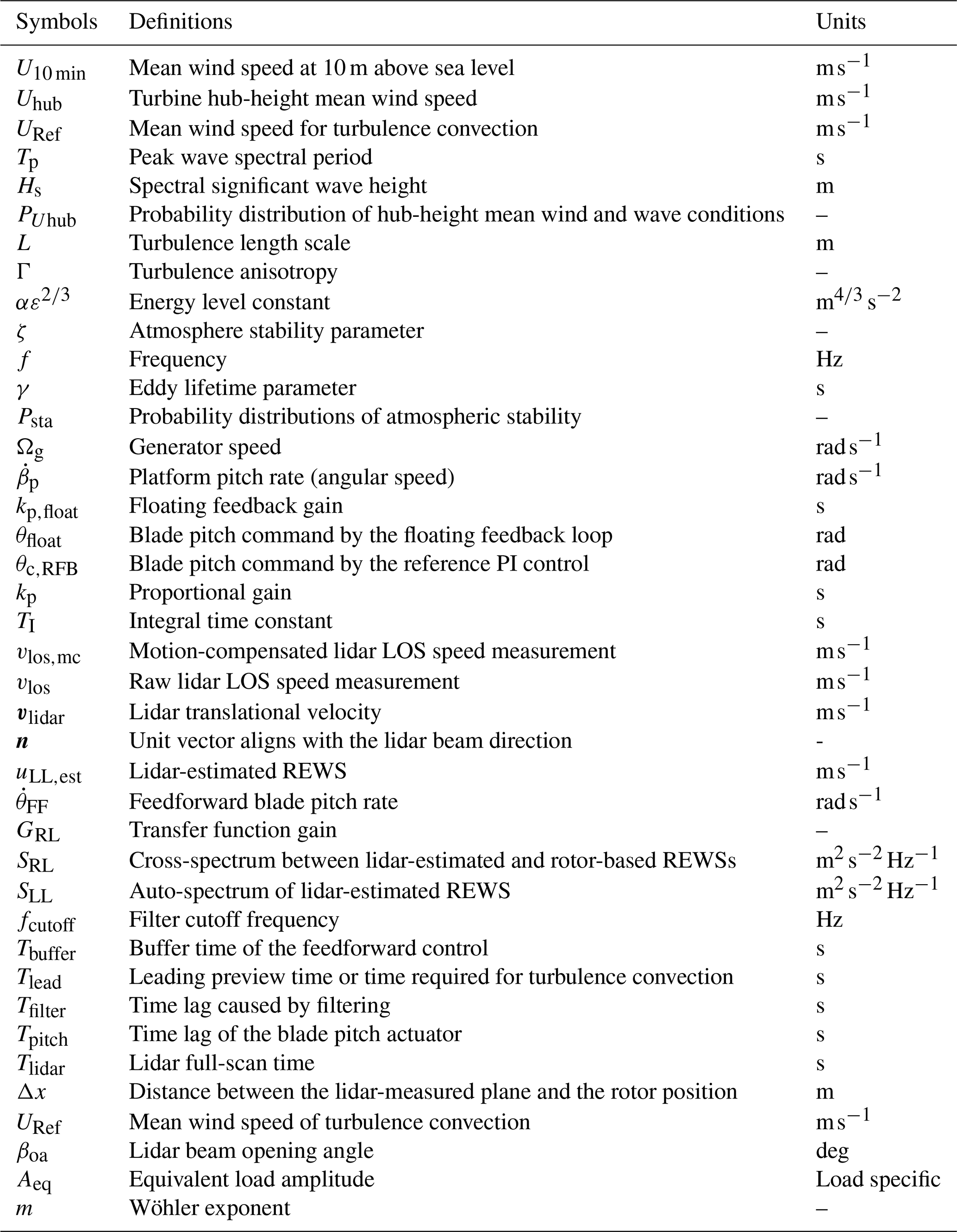
In this work, we perform optimizations of feedback gains for an MVFB control and an LACPF + MVFB control using nonlinear OpenFAST simulations. Instead of using optimization solvers as Zalkind et al. (2022) did, our optimizations rely on the simple brute-force algorithm. After optimizing control parameters, the control performances are assessed using realistic offshore turbulence characteristics and considering the variability in turbulence parameters related to atmospheric stability conditions. The main contributions of this work include (a) providing guidance towards the baseline design of lidar-assisted feedforward controls for floating turbines, (b) making comparisons between the MVFB and LACPF + MVFB controls of the optimal control tuning parameters, and (c) assessing the performance of the two controls using realistic offshore turbulence characteristics. A nomenclature of symbols used in this paper is provided in Table 1.
The rest of this paper is structured as follows: Sect. 2 provides some background on the floating turbine model, environment conditions, and lidar system; Sect. 3 illustrates the design of the MVFB and LACPF + MVFB controls; Sect. 4 presents the tuning of the feedback gains; Sect. 5 assesses the optimally tuned controls; and lastly, Sect. 6 concludes this paper and proposes further work.
This section provides background on the FOWT, wind and wave conditions, and the lidar system.
2.1 Floating wind turbine model
The IEA 15 MW semi-submersible floating wind turbine, developed collaboratively by NREL, DTU, and UMaine (Gaertner et al., 2020), is considered in this work. This reference floating turbine has a rotor diameter of 240 m and a hub height of 150 m. It uses a steel semi-submersible floating structure designed by UMaine (Allen et al., 2020). The turbine model has been made openly available on the IEA Wind Task 37 GitHub repository. The latest FOWT model built for OpenFAST version 3.0 is used in this research (https://github.com/IEAWindTask37/IEA-15-240-RWT/tree/ed7e726062a1355fd0355cdb4fba739fb682ff9e last access: 8 August 2023). A diagram of the reference turbine and the inertial coordinate system is shown in Fig. 1. The longitudinal direction (along the x axis) is considered the mean wind direction. The directions of platform motions in this work follow the right-hand rule according to the inertial coordinate system.
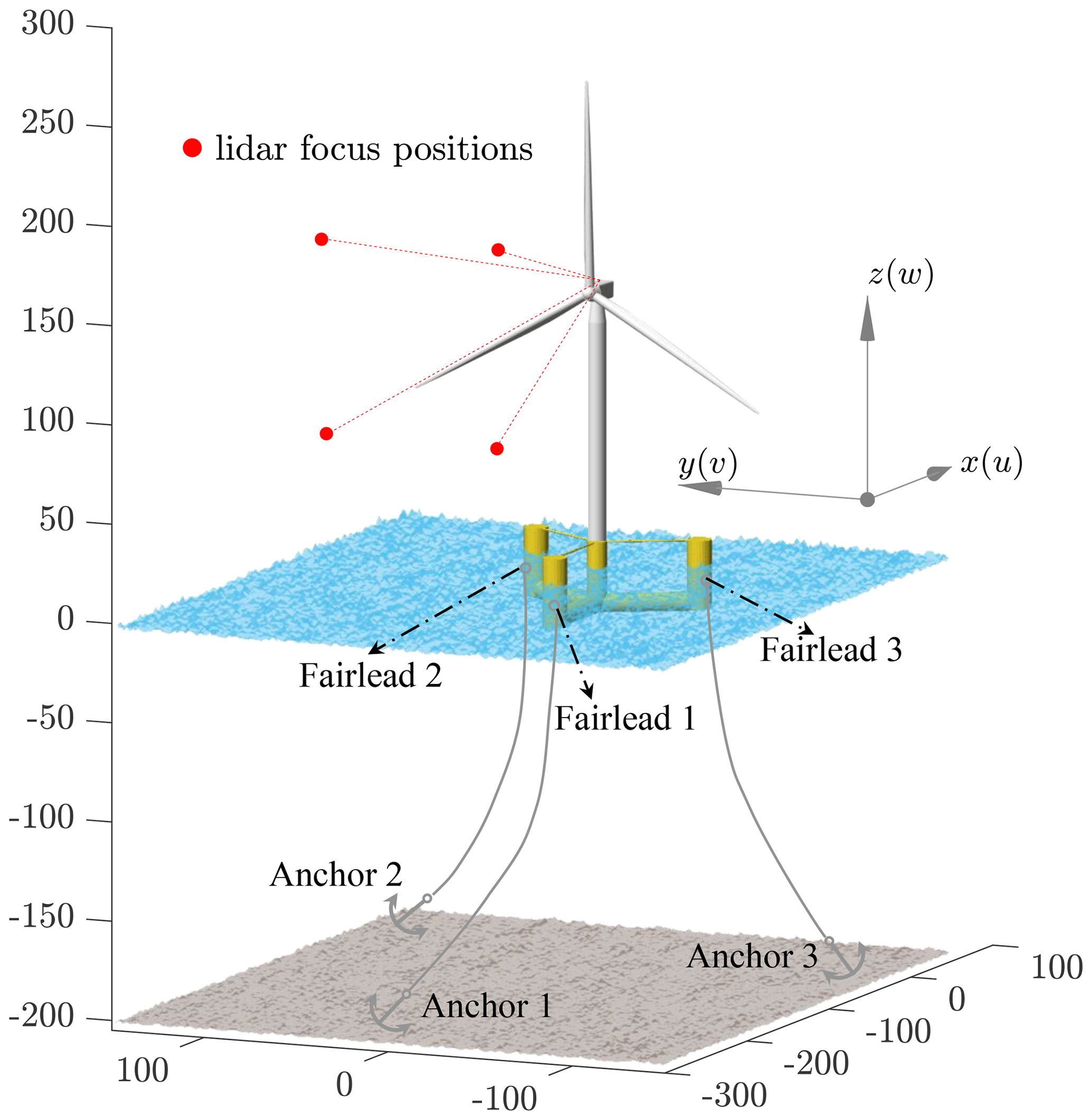
Figure 1A diagram of the investigated IEA 15 MW reference turbine equipped with a four-beam nacelle lidar system and a UMaine semi-submersible floating platform, made using the computer-aided design (CAD) data provided by the IEA Wind Task 37 GitHub repository (https://github.com/IEAWindTask37, 8 August 2023). The coordinate system follows the right-hand rule (with a unit in m) and is applicable to the full paper. Note that the positions of the anchors are not true values due to the limitations of the figure frame.
2.2 Wind and wave
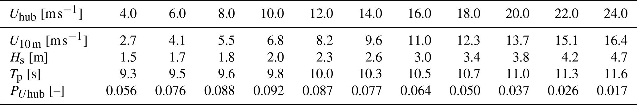
To assess the control performances using realistic offshore environmental conditions, we consider the wind and wave joint distribution, according to the study by Bachynski and Eliassen (2019). The data were selected by Bachynski and Eliassen (2019) according to the analysis of hindcast data by Li et al. (2013). The selected site corresponds to site no. 14, which is located in the North Sea and is 30 km away from the western Norwegian coast. The water depth of this site is 202 m, which is close to the design depth (200 m) of the FOWT model (Allen et al., 2020). This site data are also used by Bachynski and Eliassen (2019) to analyze the fatigue loads of FOWTs. According to Li et al. (2013), the probability distribution of the 1 h mean wind speed at 10 m above sea level (U10 m) follows a Weibull distribution with shape and scale parameters equivalent to 2.02 and 9.41, respectively. We use these Weibull parameters and assume a power log shear exponent of 0.14, as specified by the IEC 61400-1 (2019) standard, to obtain the probability distribution (PUhub) of turbine hub-height mean wind speed (Uhub), which is summarized in Table 2. The second and third rows correspond to the peak wave spectral period Tp and the spectral significant wave height Hs, respectively. For a specific mean wind speed, these are the most representative conditions (Bachynski and Eliassen, 2019). The stochastic irregular waves are generated using these two wave parameters, according to the JONSWAP spectra (IEC 61400-3, 2009).
Table 2Distributions of mean wind and wave characteristics used for aeroelastic simulations.
The extended four-dimensional (4D) Mann turbulence model (Guo et al., 2022a) is considered to model turbulent wind fields, which considers turbulence evolution. The 4D Mann model assumes stationary stochastic turbulence fields, meaning that the statistics of both upstream and downstream turbulence fields follow the statistics described by the Mann spectral tensor (Mann, 1994). The main reason for using the extended Mann model for the assessment in this work is that the lidar system needs to measure at a far distance in front of the rotor for LAC (as discussed in Sect. 3.2.2); therefore, it is not realistic to assume Taylor's frozen hypothesis (Taylor, 1938) with which the turbulence structures are assumed to be unchanged when propagating from upstream to downstream positions. More details about the 4D Mann turbulence model can be found in the work of Guo et al. (2022a).
As studied by several authors (de Maré and Mann, 2014; Cheynet et al., 2017; Peña, 2019; Putri et al., 2022), the turbulence spectral parameters can vary from the values specified in the IEC 61400-1 (2019) standard, and they change with atmospheric stability. Thus, we fit the Mann turbulence parameters, length scale L and anisotropy parameter Γ, according to the spectral analysis results of offshore FINO1 site1 data provided by Cheynet et al. (2018). The fitting process relies on minimizing the root mean square error between the FINO1 data- and the Mann-model-based spectra (see Guo et al., 2023, for the detailed fitting process). Another concern with considering the offshore turbulence spectral parameter is that these parameters are related to the lidar wind preview for turbine control (Guo et al., 2023), and the platform motion is primarily linked to the turbulence length scale for a certain turbulence intensity (TI) level. With a larger length scale, there are larger coherent turbulent eddies, and they have greater potential to excite the low-frequency platform modes more severely, resulting in higher structural loads (Bachynski and Eliassen, 2019). The three most frequent stability classes from the study by Cheynet et al. (2018) are considered in this paper. These stability classes are characterized by a stability parameter ζ related to the reference height and Obukhov length (Obukhov, 1971). Table 3 summarizes the fitted Mann parameters and the probability distribution (Cheynet et al., 2018) of the three stability classes in each mean wind speed range. In terms of the energy level constant , it is scaled to follow a TI level corresponding to the Class-C turbine specified by IEC 61400-1 (2019). The equations provided by the offshore standard IEC 61400-3 (2009) are used to calculate the standard deviations of the wind velocity components. Figure 2 shows the fitted spectra of longitudinal velocity components, where the fitted spectra generally agree with the estimated spectra from the FINO1 measurement site. Note that we only consider the frequency range with 0.001 < f<2 Hz in the fitting process and ignore the turbulence fluctuations of lower frequencies because they are less significant for the turbine motions and loads.
Table 3The Mann model parameters under different atmospheric stability conditions fitted using the spectral analysis of FINO1 data by Cheynet et al. (2018) and their probability distributions Psta [−] at different mean wind speeds. The atmospheric stability is classified by the stability parameter ζ. The energy level constant [] is scaled to follow a TI level corresponding to the Class-C turbine specified by IEC 61400-1 (2019).
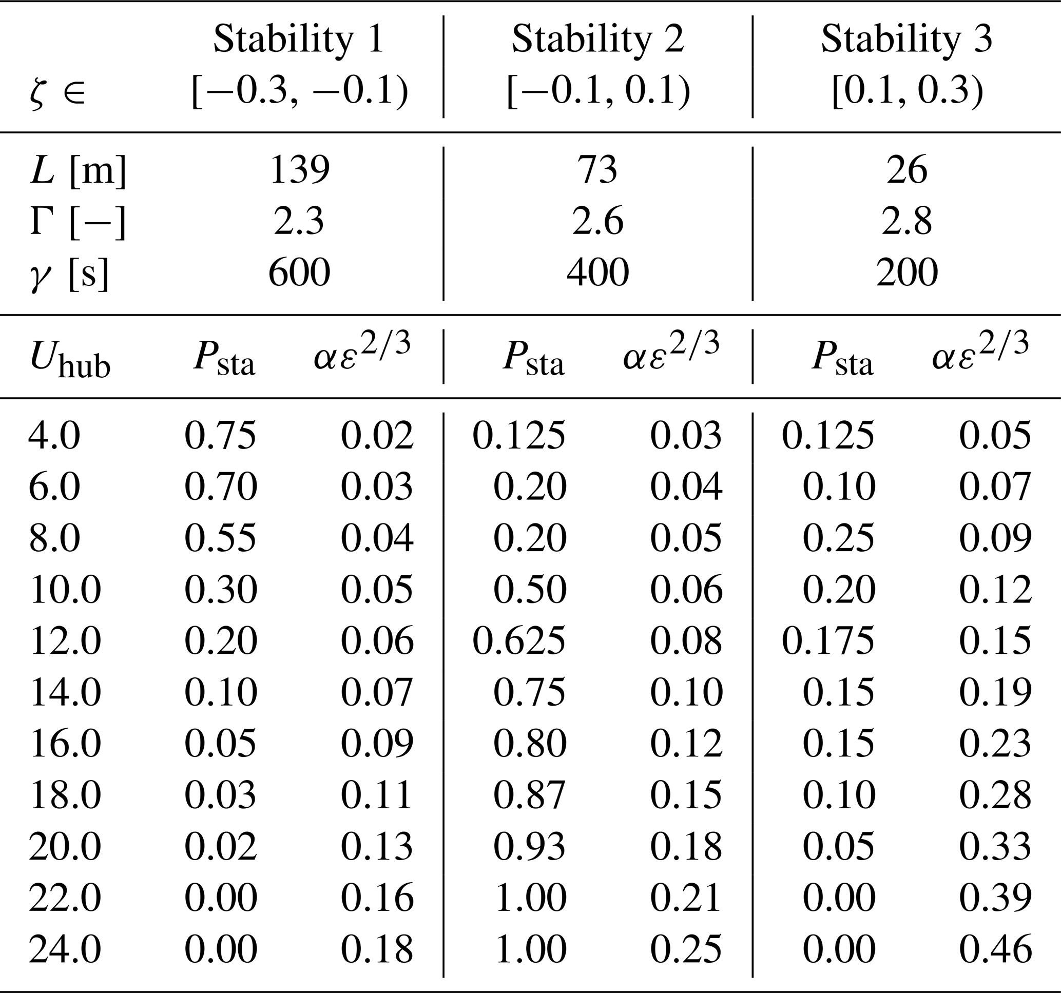
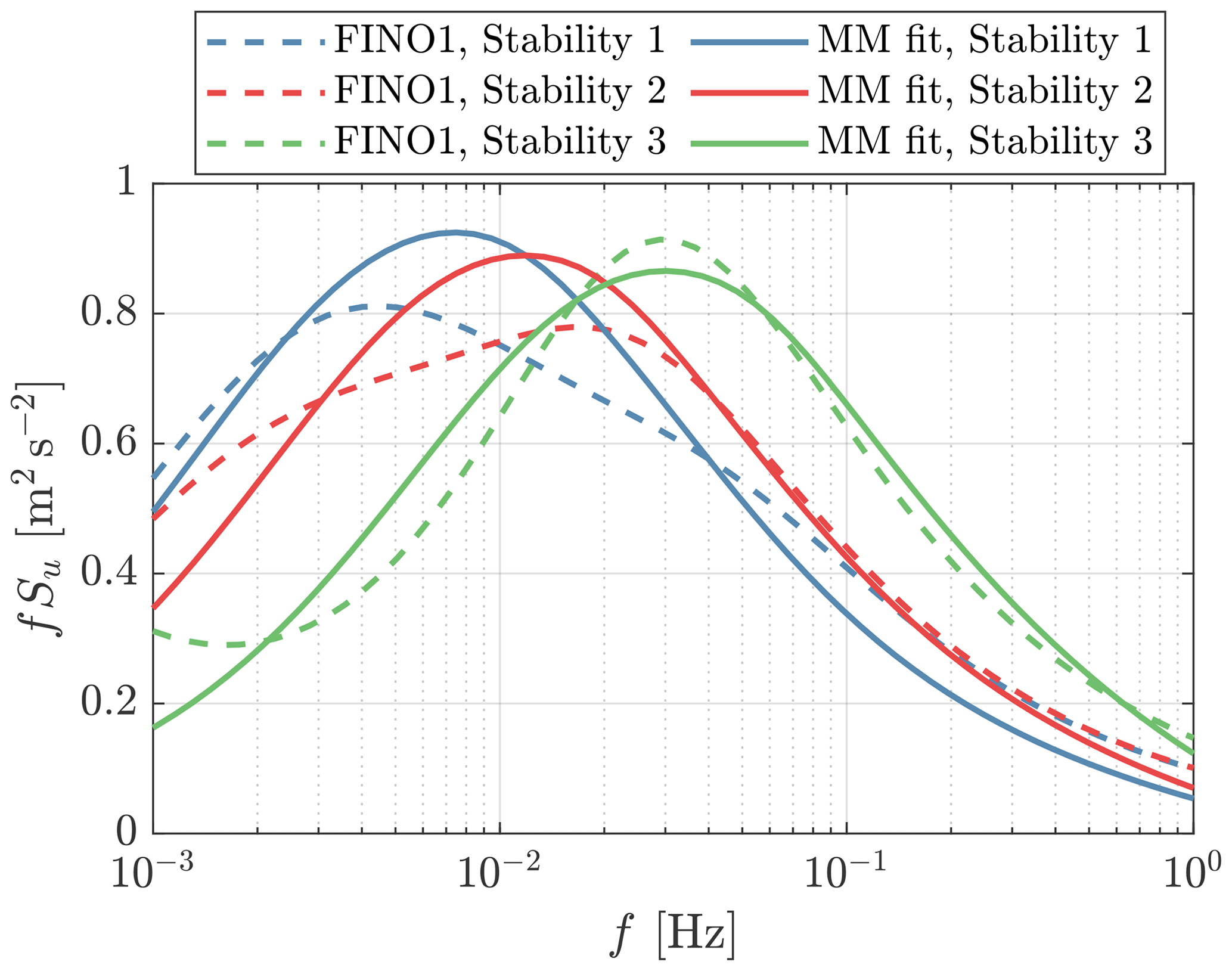
Figure 2The estimated spectra using FINO1 measurement data by Cheynet et al. (2018) and the fitted Mann-model-based spectra (indicated as MM fit in the legend). The spectra shown here are calculated assuming a mean wind speed of 16 m s−1. The spectra are normalized to have the standard deviations correspond to TI = 12 %.
In the 4D Mann turbulence model, there is an additional parameter that defines the severity of turbulence evolution, namely, the eddy lifetime γ. Thus far, there has been limited literature that has studied the distribution of this parameter under different atmospheric stability classes in an offshore environment. We chose this parameter according to the study by Guo et al. (2023), which is a summary of several works that studied turbulence evolution by onshore measurements (coastal, flat terrain). In this work, the eddy lifetimes of unstable, neutral, and stable atmospheric conditions used by Guo et al. (2023) are used for Stabilities 1, 2, and 3, respectively, because of the high similarity of the stability parameter ζ.
To perform aeroelastic simulations using OpenFAST, we generate turbulence boxes using the 4D Mann turbulence generator.2 Each 4D turbulence box has dimensions of grid points, corresponding to the time and the x, y, and z directions. The lengths in the y and z directions are both 288 m. Note that the original turbulence boxes have a dimension of 128 grid points in both the y and the z directions, but they are cropped to avoid the periodicity inherited from the 3D inverse Fourier transform (Mann, 1998). The two y–z planes in the x direction are used for simulating lidar measurements and turbine aerodynamics, respectively. Since the total number of time steps is 2048, we chose a time step of 0.293 s for the turbulence field, which leads to a total time length of 600 s. Note that the simulation time length of 600 s is selected according to the IEC 61400-3-2 (2019) standard. Similarly, the irregular waves are generated using the same time step and length as the turbulent wind. Both wind fields and waves are assumed to be periodic in time.
2.3 Lidar system
We consider a typical, commercially available four-beam pulsed lidar configuration for this study. In practice, the pulsed lidar system is able to provide measurements from different range gates along the laser direction. We only consider one measurement range gate in this work. As a result, this lidar system only relies on a simple lidar data-processing algorithm for feedforward control. Before implementing the LAC system, the lidar measurement trajectory optimization is presented in Sect. 3.2.2, which aims to find optimal opening angles of laser beams and upstream-focused distance.
To simulate a realistic lidar system in the OpenFAST environment, we use the lidar module-integrated OpenFAST version 3.0, in which a realistic lidar simulation module is updated by Guo et al. (2022b). The updated lidar module considers realistic lidar measurement properties, including the probe volume-averaging effect along the LOS direction, the contribution of the nacelle movement to the LOS measurement, laser beam blockage caused by turbine blade passing, the turbulence evolution, and the adjustable measurement availability. Under some special weather conditions, such as extreme fog, heavy rain, and an extremely clear sky, the lidar system does not always provide reliable measurements due to a low carrier-to-noise ratio caused by low backscattering. However, in this work, we ignore the low availability caused by special weather conditions and only consider the remaining three characteristics in the simulations.
In this section, we first describe the MVFB control and then discuss the design of the lidar-assisted control.
3.1 Multivariable feedback control
Apart from the generator speed Ωg, the MVFB control additionally feeds back the fore–aft-motion-related signals. Currently, ROSCO, developed by NREL, supports the MVFB control for floating turbines. A detailed description and the source code of NREL's ROSCO can be found in the work of Abbas et al. (2022) and NREL (2021). As suggested by Fleming et al. (2019), the MVFB control shows a better performance if the platform pitch angle is used in the floating feedback loop. Thus, in this work, we modified the lidar-integrated OpenFAST 3.0 and ROSCO 2.6.0 (NREL, 2021) to be able to use the platform pitch rate for the floating feedback loop, as shown in Fig. 3. In the floating feedback loop, the blade pitch angle θfloat is simply determined by
where is the band-pass-filtered platform pitch rate, and kp,float is a constant gain. Depending on the sign of the floating feedback gain kp,float, the floating feedback loop can compensate for the relative wind speed change caused by platform motion or provide damping effects to the platform pitch motion. Based on the coordinate system used in this work, a positive gain that aims for platform damping is selected. For example, a positive platform pitch motion means that the rotor is pushed backwards, which leads to an increase in blade pitch and eventually a decrease in aerodynamic thrust on the rotor.
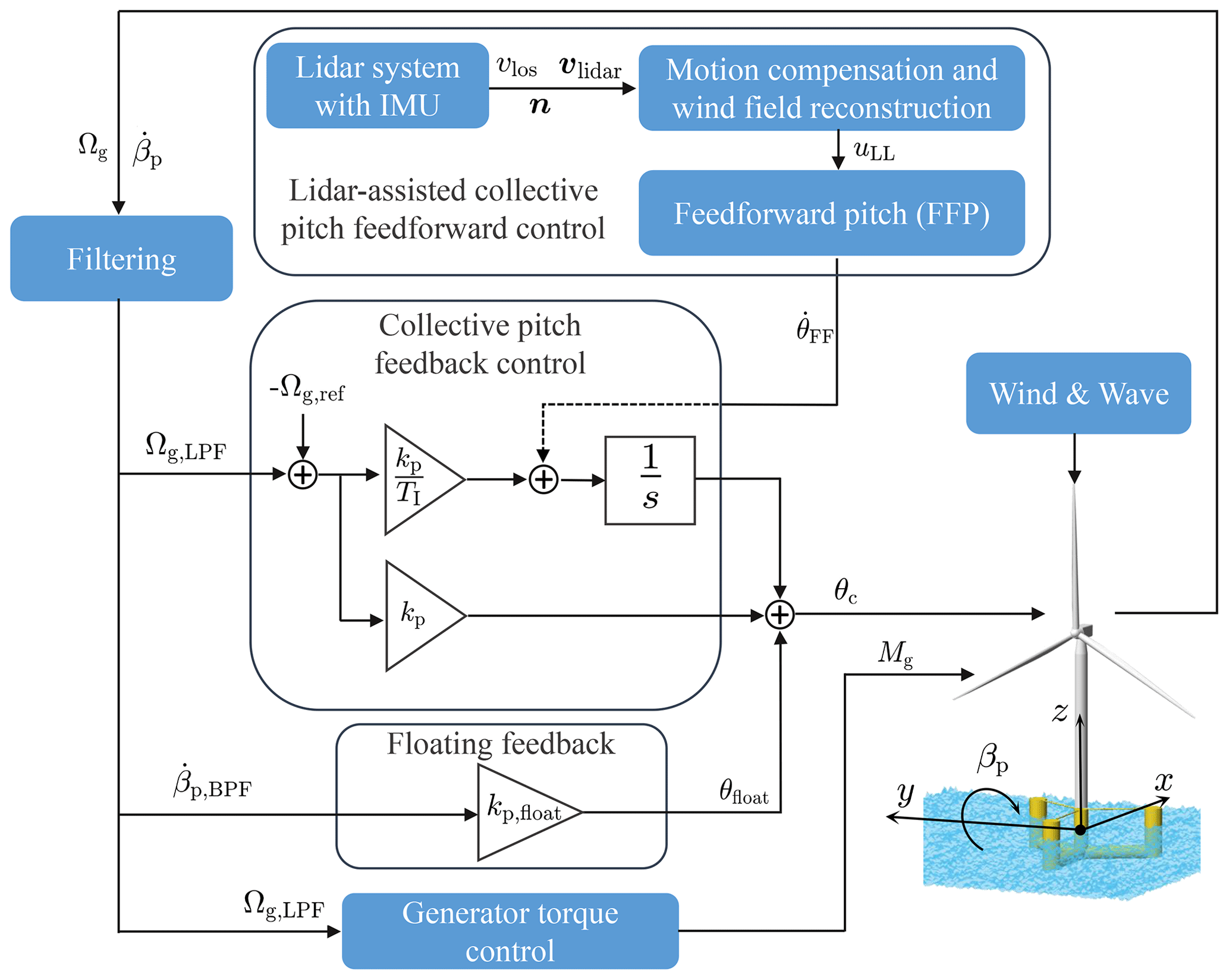
Figure 3The overall control diagram for a floating wind turbine. Note that the measured blade pitch angle (θ) signal is also used in the generator torque control and collective blade pitch feedback control modules (Abbas et al., 2022; NREL, 2021), but the lines are omitted.
As for the regular collective blade pitch feedback loop, we use the PI control already developed in ROSCO; i.e.,
where . Here, θc,RFB is the pitch command of the reference feedback-only control (without LAC), kp is the proportional gain, TI is the integral time constant, Ωg,ref is the generator speed control reference, Ωg,LPF is the low-pass-filtered generator speed, and s is the complex frequency.
Figure 4 shows the response of the IEA 15 MW floating turbine to an extreme operating gust (EOG) defined by the IEC 61400-1 (2019) standard. Here, no wave disturbance is considered in order to emphasize the response to wind disturbance. The open-loop results mean that both the blade pitch angles and the generator torque are kept constant (steady-state value). It can be observed that the open-loop system is stable after the EOG. However, with the baseline single-variable (generator speed) feedback control, the system is not stable due to the well-known “negative damping” problem of floating turbines (Jonkman, 2008; Ward et al., 2019). The system becomes stable again by introducing the floating feedback loop into the MVFB control.
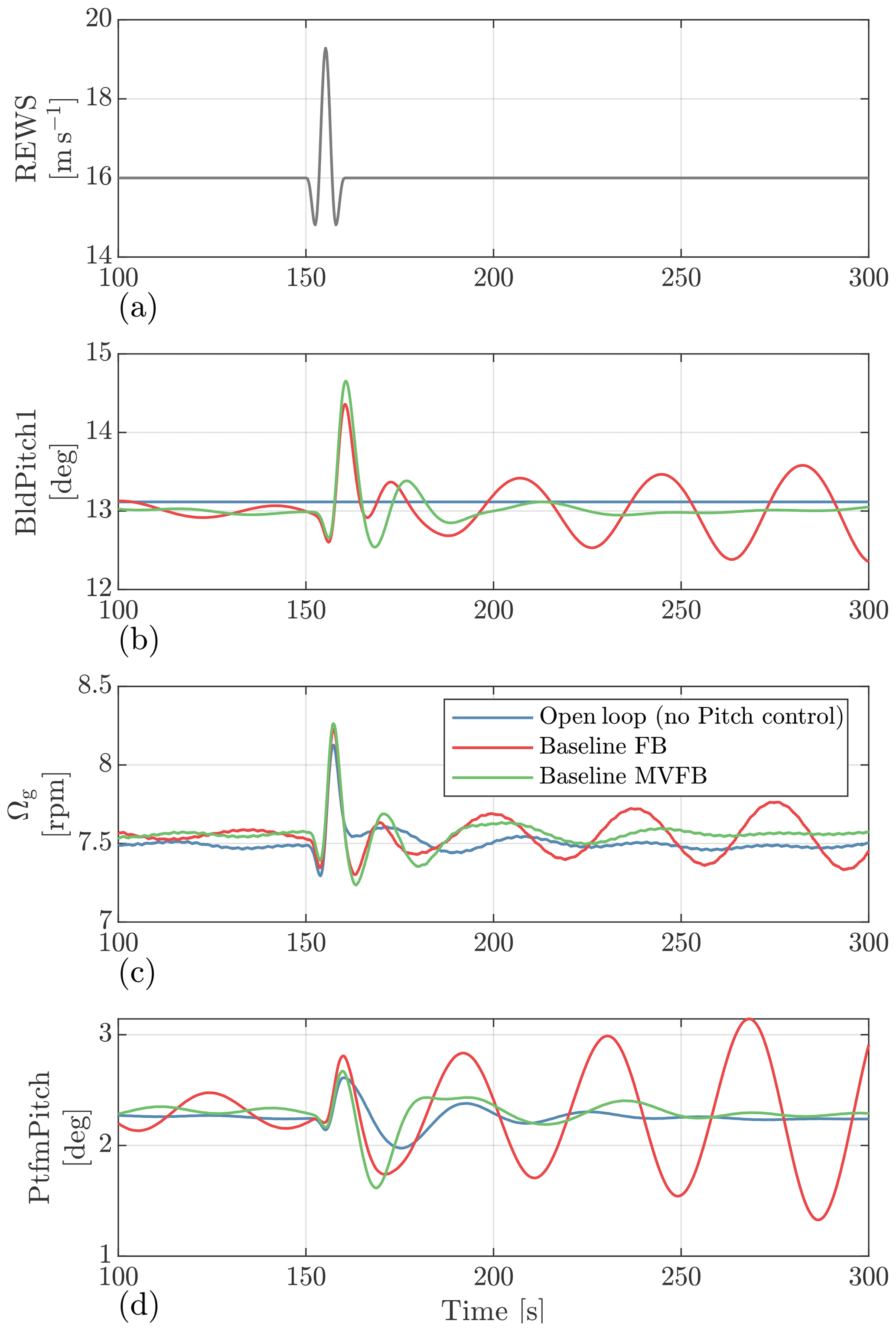
Figure 4Time series of the OpenFAST simulation responses to an extreme operating gust defined by the IEC 61400-1 (2019) standard. The baseline FB is the single-variable (generator speed) feedback control.
3.2 Lidar-assisted control
3.2.1 Control implementation
The LAC system in this work is designed for feedforward rotor speed regulation, mainly based on the work of Schlipf (2015). An open-source LAC implementation for onshore turbines has been developed by Guo et al. (2023). In this open-source LAC framework, a wrapper dynamic link library (DLL) first calls a lidar data-processing (LDP) module, then a feedforward pitch (FFP) module, and lastly the ROSCO module. All these modules are written following the Bladed-style DLL data exchange interface (DNV-GL, 2016). Compared with the onshore version of LAC, only two updates have been made for the LAC of floating turbines; therefore, we only point out the differences in this work. For a more detailed description of LAC, see the work by Guo et al. (2023) and Schlipf (2015).
First, the lidar LOS measurements are deteriorated by the nacelle motion, and the motion is much more significant in the coupled-frequency ranges close to the natural frequency of the platform fore–aft pitch mode. Therefore, the LOS measurement needs to be motion-compensated for floating turbines (Schlipf et al., 2020). For onshore turbines, the nacelle motion is mainly caused by excitation of the tower's natural frequency, which lies in the frequency range above the cutoff frequency of the low-pass filter implemented in LAC. The amplitudes of tower top motions in the onshore cases are smaller than those of the floating cases; therefore, it may not be necessary to have a compensation algorithm. Oppositely, the natural frequencies of platform modes of floating turbines are in the low-frequency range, and they are not necessarily or completely filtered out by a standard filter design of LAC. If not compensated for, the contribution of nacelle motions becomes unnecessary pitch actuation in LAC and can result in undesired control behavior. Thus, we implement a compensation algorithm assuming a perfect inertial measurement unit (IMU); i.e.,
Here, vlos is the LOS measurement at the lidar system, vlidar is the lidar translational velocity vector provided by the IMU, is a unit vector aligned with the lidar beam direction, and vlos,mc is the LOS speed after motion compensation. The unit vector n can simply be calculated after knowing the azimuth angle ϕ and elevation angle β of the lidar beam. We assume the positive x axis has zero azimuth, and the positive z axis has 90∘ elevation. After motion compensation, the identical wind field reconstruction algorithm used by Guo et al. (2023) is applied in this work to obtain the lidar-estimated REWS uLL,est.
Second, in the previous FFP module by Guo et al. (2023), only a low-pass filter was applied to the lidar-estimated REWS. In this work, a notch filter is additionally introduced into the FFP module for the LAC of floating turbines. The main reason for the notch filter is to avoid conflict with the floater damping control in the MVFB control. The floater damping is tuned to add a damping effect to the floater's fore–aft pitch motion by changing the rotor thrust force, but the LAC aims to compensate for the change in aerodynamic torque. In the above-rated operation of typical turbine rotors, when the blade pitch is adjusted, both aerodynamic torque and rotor thrust increase or decrease together so that only one control objective can be achieved. Therefore, the notch filter is designed to have a cutoff frequency of 0.029 Hz, which is the natural frequency of the floating pitch motion. After low-pass and notch filtering the lidar-estimated REWS, the FFP module sends a blade pitch rate signal to the integrator of the collective pitch control, as shown in Fig. 3. Thus, the overall pitch command of the lidar-assisted feedforward multivariable feedback control becomes
3.2.2 Lidar trajectory optimization
Due to several inherent characteristics, such as the misalignment to the longitudinal direction, turbulence evolution, and non-continuously available measurements, the lidar system does not provide a perfect estimation of the REWS (Guo et al., 2022a). However, with a reasonable lidar data-processing algorithm, it is able to provide a REWS that estimates the low-frequency variation in the actual effective wind speed acting on the rotor well. The quality of lidar preview can be defined by the following transfer function (Schlipf, 2015; Simley and Pao, 2013; Guo et al., 2023):
where SLL is the auto-spectrum of lidar-estimated REWS, and SRL is the cross-spectrum between lidar-estimated and rotor-based REWSs. An analytical solution of SRL and SLL for specific Mann turbulence parameters, turbine rotor size, and lidar trajectory configuration has been derived by, e.g., Mirzaei and Mann (2016), Held and Mann (2019), and Guo et al. (2022a, 2023). In practice, a first-order linear low-pass filter is designed to have a cutoff frequency fcutoff, which corresponds to the frequency where the transfer function reaches −3 dB (Schlipf, 2015; Simley et al., 2018). A higher value of fcutoff indicates that more frequency components in the lidar-estimated REWS can be used for feedforward pitch control.
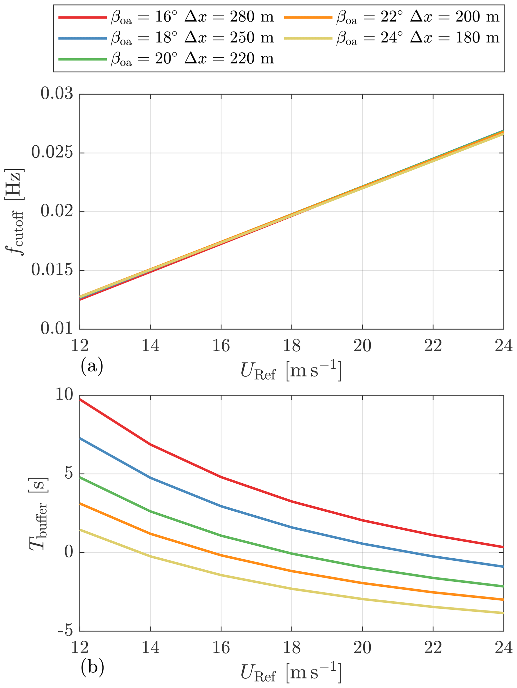
Once the cutoff frequency of the low-pass filter is determined, a buffer time Tbuffer can further be determined, which ensures the feedforward pitch command is activated at the proper time. Tbuffer can be calculated by (Schlipf, 2015; Guo et al., 2023)
where Tlead is the time required by turbulence fields to propagate the lidar-focused position to the rotor plane (also called leading time), Tpitch is the time delay of the pitch actuator, Tlidar is the lidar full-scan time, and Tfilter is the time delay caused by low-pass and notch filtering. For the four-beam lidar considered here, Tlidar equals 1 s because each beam direction takes 0.25 s to finish measurement. Tlead can be approximated by , where Δx is the distance between the lidar-measured plane and the rotor position, and URef is the mean wind speed of turbulence convection (usually assumed to be Uhub). The time delays of the pitch actuator and filter can both be calculated using the frequency responses of their transfer functions as
where θfilter and θactuator are the lagging-phase responses of the filters and pitch actuator transfer functions in degrees, respectively. They are both functions of frequency, and the values at 0.025 Hz are chosen for the IEA 15 MW turbine because this is the critical frequency near where the rotor has higher fluctuations. In the used ROSCO (version 2.6.0), the pitch actuator of the 15 MW turbine is modeled as a second-order system with a natural frequency of 0.25 Hz and a damping ratio of 0.7 (Abbas et al., 2022).
Because Stability 2 in Table 3 has a dominant probability of occurrence, we choose its turbulence parameters and consider the IEA 15 MW turbine rotor with a four-beam pulsed lidar to calculate fcutoff under different lidar trajectory configurations. The four lidar beam directions are assumed to have an identical opening angle βoa with the negative x-axis direction, and their projections on the y–z plane have angles of 45, 135, 225, and 315∘ to the positive y axis. The optimization variables are the opening angle of the four beams and the focused upstream distance Δx. With the discussion above, the lidar trajectory optimization problem can be formulated as
To find an optimal trajectory defined by the opening angle βoa and the focused distance Δx, several discrete configurations are considered. For each above-rated wind speed from 12 to 24 m, we calculate fcutoff and Tbuffer, considering βoa varying from 16 to 24∘ with a step of 2∘ and Δx varying from 120 to 300 m with a step of 10 m. Figure 5 shows the cutoff frequencies of low-pass filters under various lidar measurement trajectories for a mean wind speed of 16 m s−1. It can be seen that the maximum cutoff frequency for a smaller opening angle βoa appears at a farther focused distance Δx. The maximum cutoff frequency of different opening angles is generally similar.
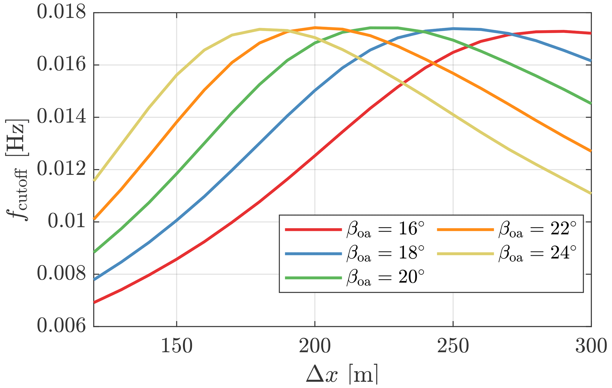
Figure 5The cutoff frequencies of low-pass filters for lidar-assisted control under various lidar measurement trajectories, calculated with a mean wind speed of 16 m s−1.
In Fig. 6, we show the cutoff frequency and buffer time as a function of the mean wind speeds to further help us select the optimal trajectory. Here, we only select the lidar trajectories that have a peak cutoff frequency in Fig. 5. In Fig. 6a, it can be seen that the cutoff frequencies vary linearly with the mean wind speed, and there are no observable differences in the compared lidar trajectories. However, in Fig. 6b, there are obvious differences in the buffer time. When the buffer time is negative, it means that the lidar-estimated REWS is too late in time after data processing and filtering such that it contradicts the feedforward control concept; therefore, trajectories with a negative buffer time at the above-rated wind speeds should be avoided in principle. In the end, the trajectory with and Δx=280 m is chosen as the optimal for our analysis later in this paper.
In this section, we perform aeroelastic simulations with various feedback gains to find the optimized values. The optimal gains bring a lower tower base fore–aft bending load, do not lead to rotor overspeed under extreme turbulence conditions, and do not lead to a significant increase in the load on other turbine components.
4.1 Rotor speed feedback gains
To find the optimized gains for the PI control in the above-rated conditions, we consider the Stability 2 condition with Uhub values varying from 10 to 24 m s−1 listed in Table 3 and perform simulations with different kp and TI values. Although the rated wind speed of the IEA 15 MW turbine (Gaertner et al., 2020) is 10.59 m s−1, the Uhub = 10 m s−1 condition is considered to find the initial gains for gain scheduling. For each mean wind speed condition, the value of kp is varied from 0.2 to 1.4 s with a step of 0.2 s, and the value of TI is varied from 5 to 20 s with a step of 5 s. We selected the variation ranges of these gains following the studies by Lemmer et al. (2020) and Zalkind et al. (2022). As for the step size selection, we consider the time consumption of the simulation and make some compromises. The overall number of simulation cases and, hence, the time required, will increase dramatically if a smaller step size is chosen. However, Fig. 7 shows that the step size we chose clearly indicates trends in tower loads. The floating feedback loop gain kp,float is considered to be 10 s in these simulations, which is further optimized in the next section. Also, the feedback gains only depend on the mean wind speed in these simulations.
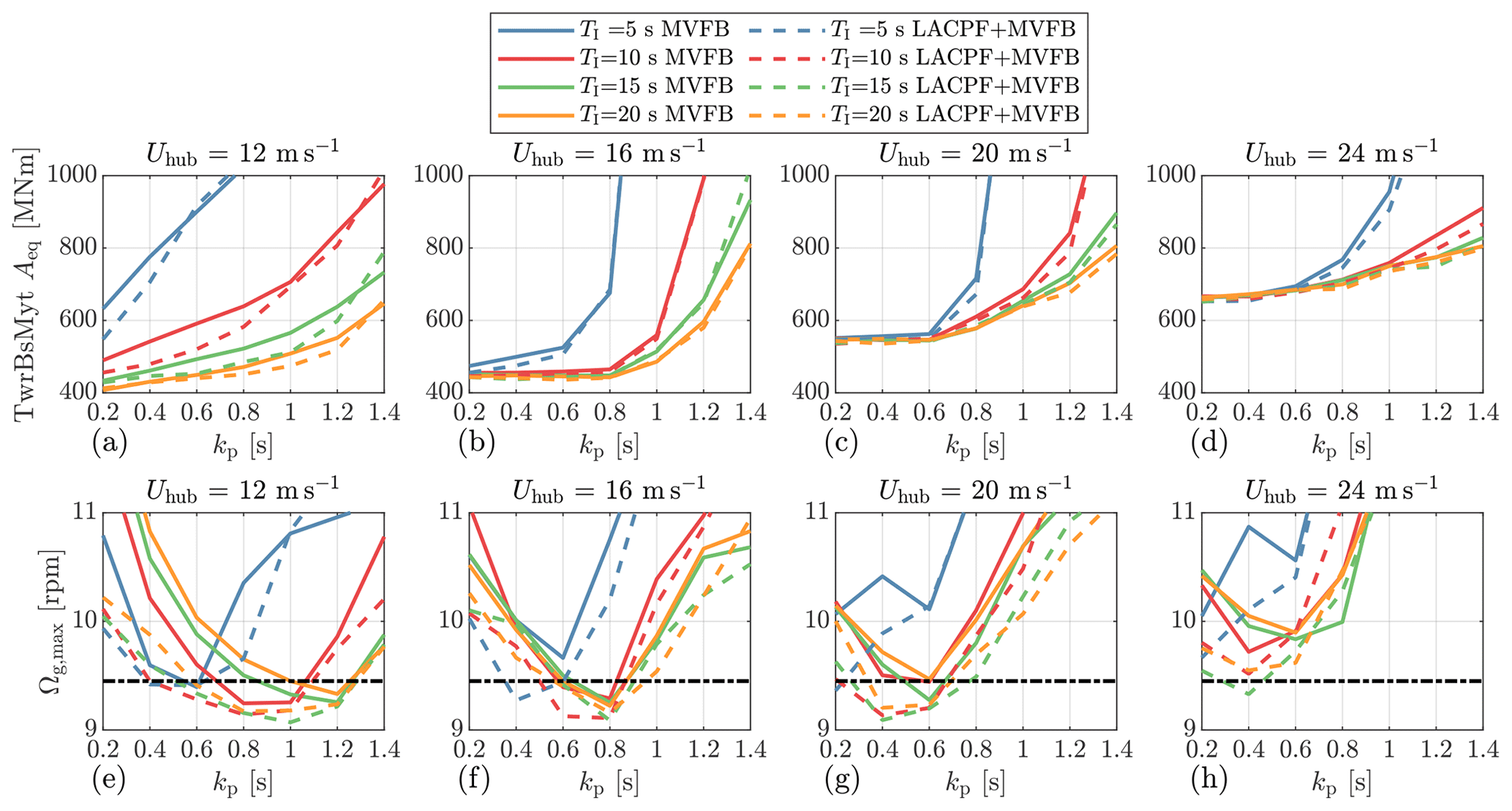
Figure 7Comparisons of equivalent tower base fore–aft bending moment amplitudes and maximum generator speeds under different gains of the PI control, simulated using turbulence spectral parameters from Stability 2. The dashed, dark line indicates an overspeed threshold. Only four representative mean wind speed conditions are shown.
For each mean wind speed with specific kp and TI values, six independent simulations are performed that have different random seed numbers for generating turbulence and waves. Also, we perform simulations for design load cases (DLCs) 1.2 and 1.3 (IEC 61400-1, 2019). For each DLC with the variations discussed above, there are 1344 simulation cases in total. Each simulation case is executed for 700 s using the periodic turbulence fields and waves, and the initial 100 s results are ignored.
For the results of DLC 1.2, we collect the time series and apply the rainflow-counting method (Matsuishi and Endo, 1968) to get load amplitudes (Ai) and the numbers of cycles (ni). After that, the equivalent load amplitude is calculated by
according to the Palmgren–Miner linear damage hypothesis, where m is the Wöhler exponent. In this work, m=4 is considered for the tower and shaft loads, m=10 is considered for the blade loads, and m=3 is considered for the mooring chain loads (Barrera et al., 2020). The average value of Aeq by six random seeds is eventually calculated and used as an indication for selecting the optimized gains. The definition of Aeq is that if a stress with an amplitude of Aeq is applied to the material once, the resulting damage is equivalent to that caused by the stochastic load. As for the results of DLC 1.3, we collect the maximum values of the results of different seeds.
Figure 7 shows the equivalent load amplitudes of tower base fore–aft bending moments (TwrBsMyts) and maximum generator speeds by different PI gains under three mean wind speeds as examples. Here, the dashed, dark line indicates an overspeed threshold, which should be avoided during turbine operation and is chosen to be 125 % of the rated generator speed (Zalkind et al., 2022). In general, a higher kp results in higher tower load amplitudes because the proportional control is more aggressive in regulating the rotor speed by adjusting blade pitch angles; therefore, the rotor thrust force varies more. For a lower mean wind speed, a larger kp is required to avoid rotor speed exceeding the 125 % threshold, which is similar to the observations by Zalkind et al. (2022). A smaller integral time constant also results in higher loads since the integral control is more sensitive under the same proportional gain. It would be preferred to use a larger TI for load reduction.
Comparing the solid and dashed lines, using LACPF control leads to lower load amplitudes and smaller maximum values of generator speed than using the MVFB control. With the MVFB control, it is observed that none of the gains satisfies the rotor speed maximum limit for a very high mean wind speed of 24 m s−1. However, when kp= 0.4 s and TI= 15 s, introducing the LACPF control limits the maximum generator speed within the selected threshold.
Overall, we select the gains according to the following criteria: (a) the maximum rotor speed is smaller than the threshold, and (b) the gains result in the smallest load amplitude, and they satisfy (a). In the case of the MVFB control, where (a) can not be satisfied, the gains that result in the smallest maximum rotor speed are selected. Figure 8 shows the selected optimal gains, the corresponding scheduled gains by interpolation, and the baseline gain scheduling provided by the ROSCO toolbox (https://github.com/NREL/ROSCO, last access: 8 August 2023) (Abbas et al., 2022) developed by NREL. Note that the blade pitch angle is used for gain scheduling in the baseline ROSCO MVFB control, and the mean wind speed is used for the optimally tuned MVFB and LACPF + MVFB controls. The baseline gain scheduling is compared with the optimal gain scheduling in Sect. 5. With the LACPF control, it is clear that the PI control can be less aggressive, especially in the range slightly above the rated wind speed.
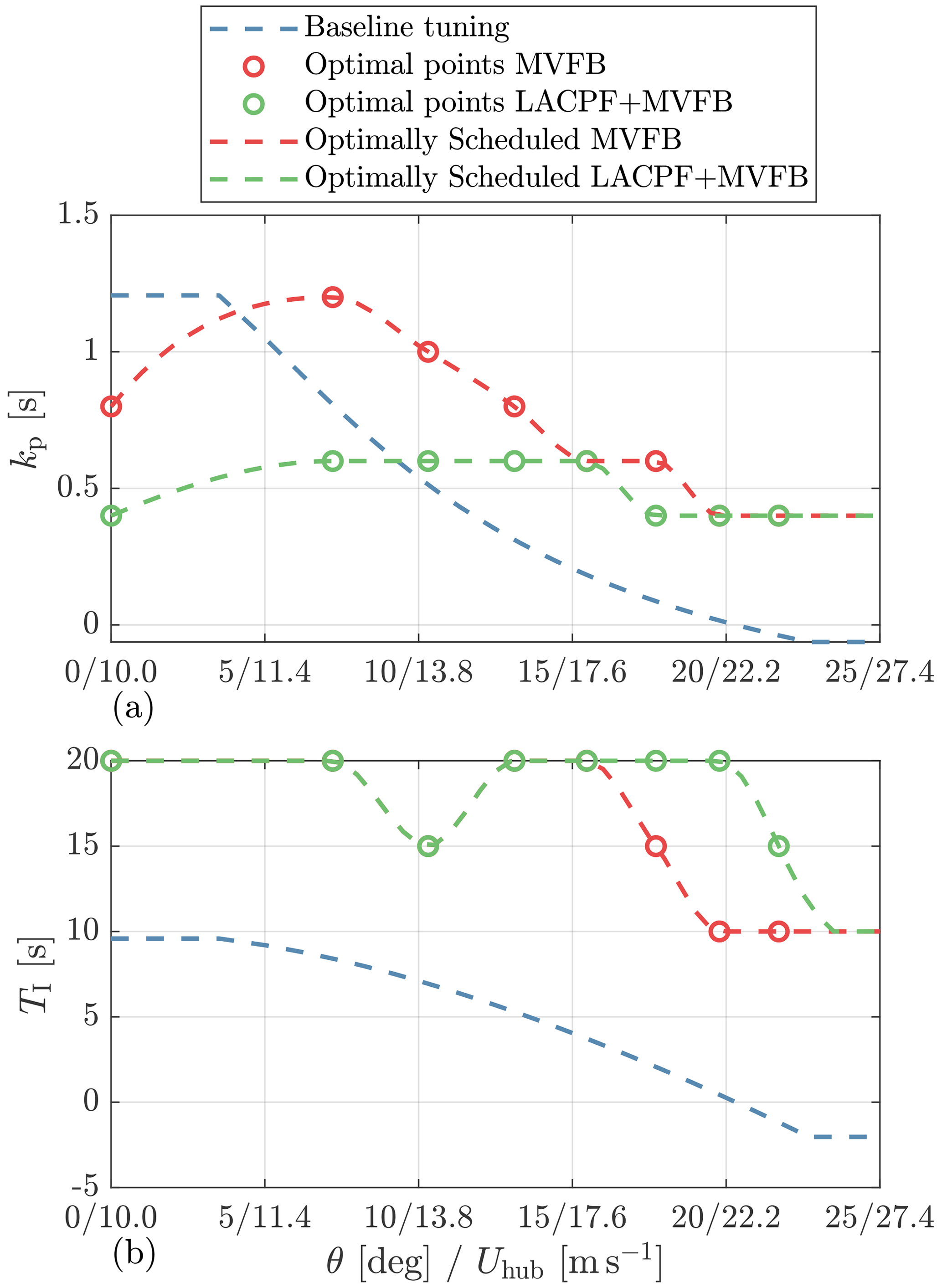
Figure 8The selected optimal gains and the gain scheduling curve for the PI control are shown. The baseline tuning is provided by the ROSCO toolbox. In the baseline ROSCO tuning, the gains are scheduled according to the measured and low-pass-filtered blade pitch angle. In the optimally tuned MVFB and LACPF + MVFB controls, the gains are scheduled by the hub-height mean wind speed.
4.2 Platform feedback gain
In this section, the floating platform pitch feedback gain is further optimized.
We perform simulations for DLC 1.2 using the PI gains obtained from Sect. 4.1, with kp,float ranging from 0 to 30 s or 20 s with a step of 2 s. The kp,float values above 20 s are not considered for very high mean wind speeds because they result in a significantly high blade pitch rate. Here, only the DLC cases with a mean wind speed above 10 m s−1 are considered. The Aeq, standard deviation (SD), and energy production (EP) are calculated and then compared. Similarly to the calculation of Aeq, the average value of standard deviations and energy productions by six random seeds is computed.
To clearly show the control performances of different kp,float values, we calculate the relative change from the case 0 s, which means no floating feedback is considered. The considered variables are some of the most important ones for a floating turbine, i.e., the tower base fore–aft bending moment, the low-speed shaft torque (LSShftTq), the blade 1 root out-of-plane bending moment (RootMyb1), the collective blade pitch velocity (BldPitchRate), and the platform fore–aft pitch motion (PtfmPitch). The blade pitch rate is considered because it is related to the damage to the blade pitch gear and bearing (Guo et al., 2023).
Figure 9a–d show the results simulated using the MVFB control with optimal PI control tuning. In general, the SDs of blade pitch rates show parabolic patterns. At the bottom of the parabolic, the blade pitch rate is minimal, meaning the reduction in the blade pitch activities is the best. As kp,float increases, the tower load and platform motion generally tend to be lower, except for the case with a mean wind speed of 14 m s−1. However, their gradients become very small for high values of kp,float. As for the blade and shaft loads, there are also valley points at which the kp,float values are close to the kp,float at the trough of the blade pitch rate. Except in the case with a mean wind speed of 14 m s−1, there is negligible dependence of EP on different floating feedback gains.
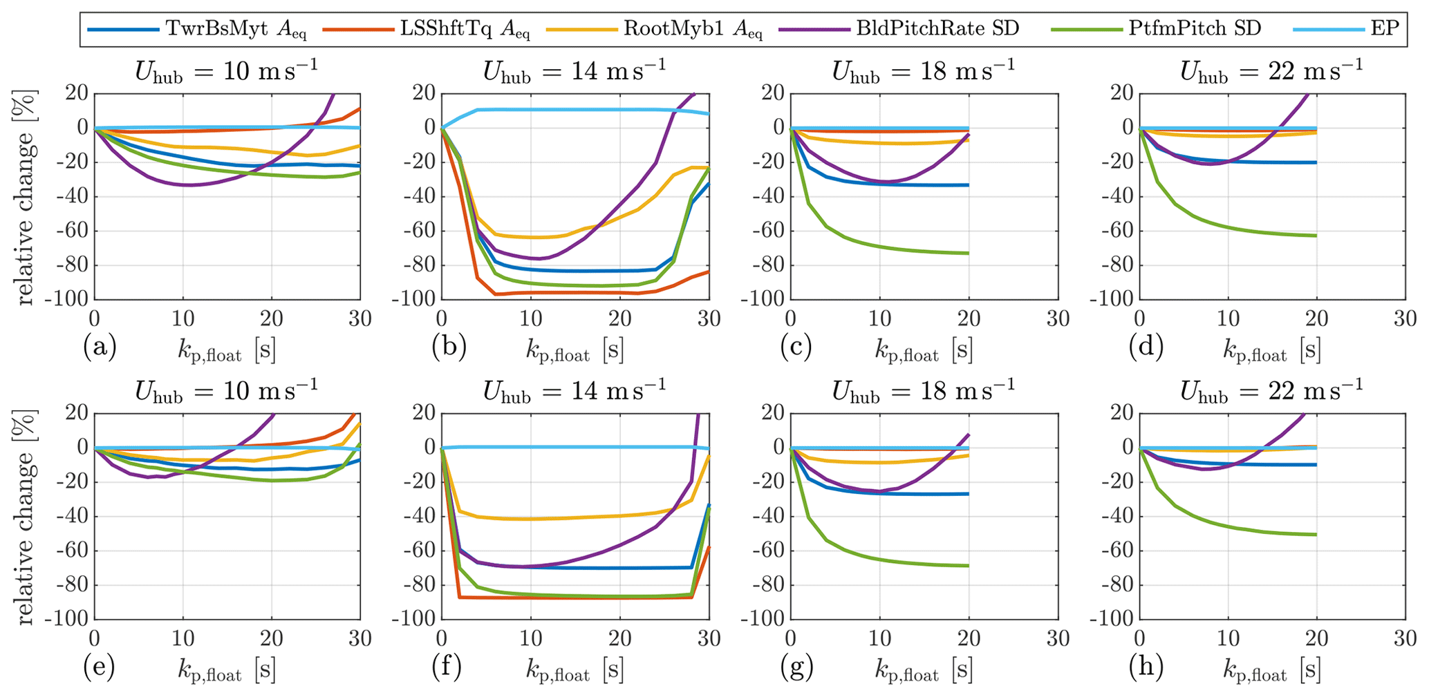
Figure 9Relative changes in equivalent load amplitudes, standard deviations, and energy production under different gains of the platform feedback loop, simulated using turbulence spectral parameters from Stability 2 on the basis of DLC 1.2. Only four representative mean wind speed conditions are shown. (a–d) The MVFB control using optimal PI control tuning. The results are relative to the case 0 s. (e–h) The LACPF + MVFB control using optimal PI control tuning. The results are relative to the case 0 s.
Figure 9e–h show the results simulated using the LACPF + MVFB control with optimal PI control tuning. In general, the relative changes show a similar trend to that simulated using the MVFB control. For a mean wind speed equal to 10 m s−1, the main difference is that the trough of the blade pitch rate appears at a smaller kp,float value in the LACPF + MVFB control than in the MVFB control.
For both MVFB and LACPF + MVFB controls, at a mean wind speed of 14 m s−1, it can be observed that the reductions in all variables are especially significant if the floating feedback gain is considered. The floating feedback loop, in particular, increases the EP in the MVFB control scenario. The above phenomena are caused by the fact that at this mean wind speed, instability occurs if kp,float = 0 s. For this special case, some examples of time series from one of the six random simulations are provided in Appendix A. In this mean wind speed condition, the control performances of both MVFB and LACPF + MVFB controls are better with kp,float between 10 and 20 s. When the floating feedback gain is too aggressive (> 25 s), the control performance reduces, which might be caused by the fact that the fore–aft motion is more sensitive to the blade pitch changes at this operating point.
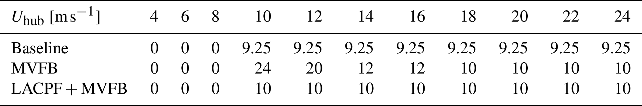
Therefore, based on the discussions above, it is preferable to select kp,float where all the structural loads and blade pitch rates are small. The corresponding kp,float values fulfilling the criteria above are those close to the trough of the blade pitch rate. Although a very high kp,float helps to reduce the platform pitch further, this is undesirable because the structure loads can be higher or marginally reduced, while the blade pitch rate becomes much higher. Table 4 summarizes the optimally selected floating gains that are scheduled as a function of the mean wind speed. In addition, the value provided by the ROSCO toolbox (Abbas et al., 2022) is used for the baseline control configuration.
Table 4The baseline and optimal (MVFB and LACPF + MVFB) floating platform feedback gains kp,float for three control configurations.
In this section, we assess the performances of the three controls: (a) the baseline MVFB control with ROSCO tuning, (b) the MVFB control with optimal tuning, and (c) the LACPF + MVFB control with optimal tuning. Three different groups of turbulence spectral parameters representing realistic offshore turbulence characteristics are considered in the fatigue assessment of DLC 1.2, as listed in Table 3. The spectral parameters for Stability 2 with a higher probability are considered for maximum value evaluations of DLC 1.3.
5.1 Performance under different environmental conditions
The maximum generator speed, platform pitch, platform surge, and blade tip out-of-plane deflection simulated by the three control configurations are shown in Fig. 10. These results are obtained from the DLC 1.3 simulations. Compared with the baseline tuning of the MVFB control, the optimally tuned MVFB control generally has a lower maximum generator speed overshoot. However, the maximum values at very high wind speeds (> 20 m s−1) are above the defined threshold (dashed, dark line). The observations here agree with the optimizations in Fig. 7. It is also observed that the optimal PI gains chosen to limit the generator speed generally have lower values of the maximum platform pitch and blade deflection than the results of the baseline gains. As for the maximum surge, the values obtained by optimal tuning are similar to those obtained by baseline tuning. The maximum values obtained by introducing the LACPF control into the MVFB control are overall similar to that resulting from the optimally tuned MVFB control. Especially for very high wind speeds, the maximum generator speed, platform pitch, and blade tip out-of-plane deflection simulated using the optimally tuned LACPF + MVFB control are slightly lower than those simulated using the optimally tuned MVFB control. The generator speed threshold is not surpassed with the assistance of lidar systems.
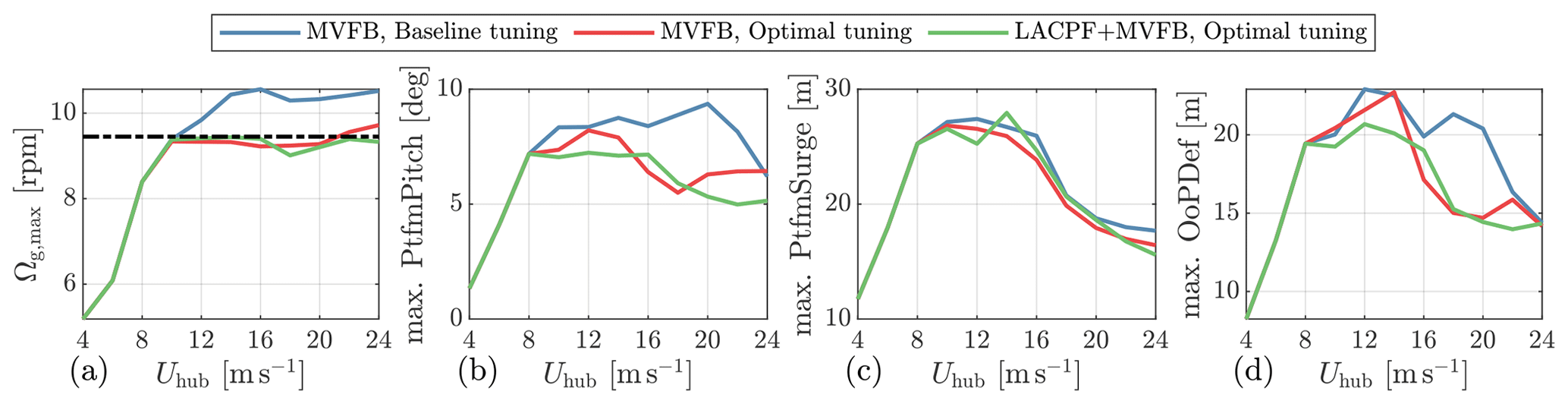
Figure 10The maximum values of some key variables for secure operation collected from DLC 1.3, simulated using the turbulence spectra parameters of Stability 2.
Figure 11 shows the relative changes in some important variables by optimally tuned MVFB and LACPF + MVFB controls relative to the baseline-tuned MVFB control. As for stability classes 1 and 3, the simulations are executed excluding the cases with mean wind seeds higher than 20 m s−1 due to their very low probability of occurrence. Note that the first fairlead tension (FAIRTEN1) is selected for comparison.
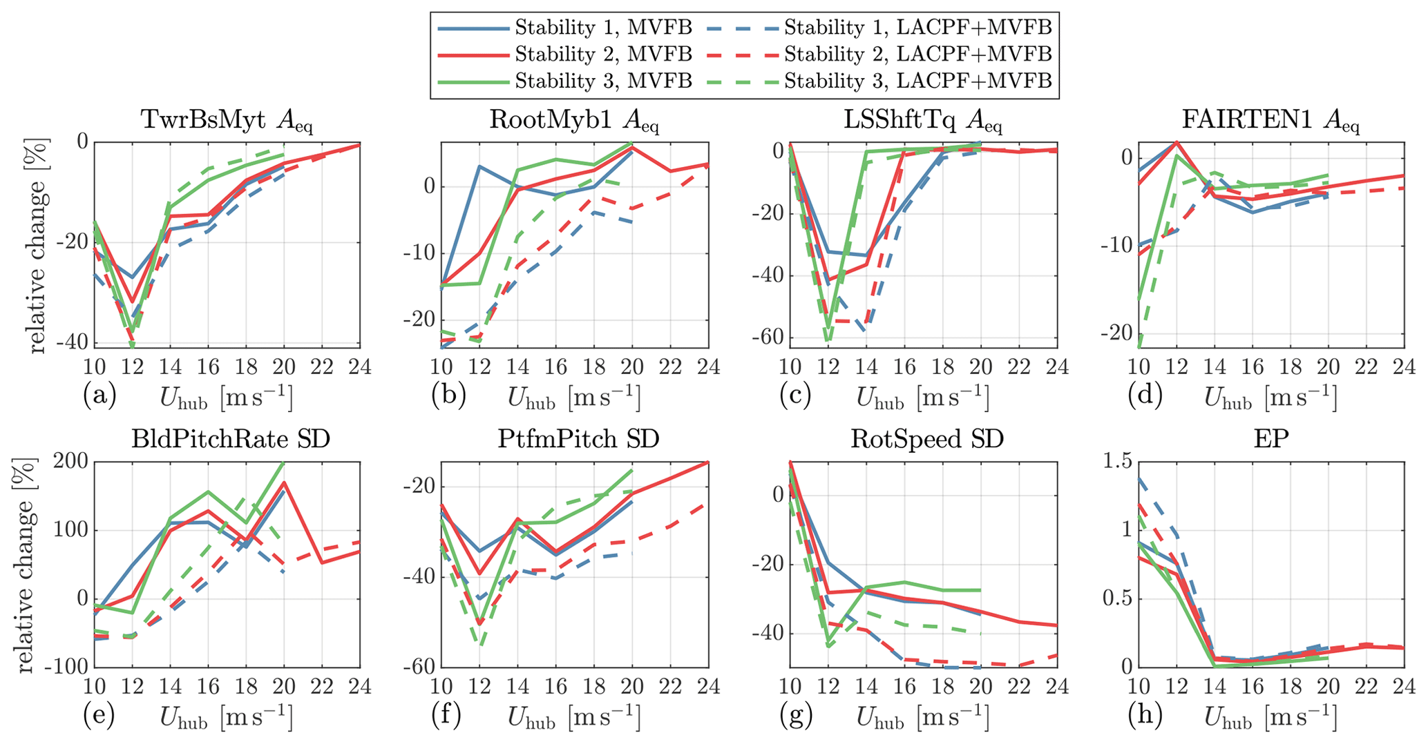
Figure 11Relative changes in equivalent load amplitudes, standard deviations, and energy productions under different mean wind speeds obtained from the DLC 1.2 simulations. The relative changes are calculated using the results of the optimally tuned MVFB and LACPF + MVFB controls relative to those of the MVFB control with baseline tuning.
Considerable load reductions are achieved in the tower, shaft, and mooring fairlead using the optimally tuned controls. However, a small increment in fairlead tension load is observed for the optimally tuned MVFB control. Decrements in platform pitch and rotor speed are also significant with optimal tuning. On the contrary, the EPs are slightly increased, and the increments are more observable closer to the rated wind speed. In terms of the blade pitch activities, the optimally tuned MVFB control gives higher blade pitch rates, which are even doubled for very high mean wind speed ranges.
Comparing the performances between the optimally tuned LACPF + MVFB and MVFB controls, LACPF + MVFB generally surpasses MVFB controls. More load reductions, higher EP increments, and lower blade pitch consumption are observed in the LACPF + MVFB control. Although the LACPF control module is designed using the turbulence spectra parameters from Stability 2, these benefits are generally observed in other stability conditions as well. In particular, the tower load at the LACPF + MVFB control is slightly higher than at the MVFB control in Stability 3 but only at very high wind speeds, where the probability of Stability 3 is much lower than that of Stability 2. Also, using the LACPF + MVFB control clearly reduces the blade pitch rate SD close to the rated mean wind speed. In addition, the increment in blade pitch rate by the LACPF + MVFB control is much lower than that by the MVFB-only control.
5.2 Evaluating lifetime performance
For a clearer indication of the control performances, we calculate the lifetime damage equivalent load (DEL) and annual energy production (AEP) as
and
Here, i and j are index numbers for mean wind speeds and stability classes. The number is the number of 10 min durations per year, and Nref is a reference cycle number chosen to be 26 (Schlipf, 2015). The designed turbine lifetime is considered to be 20 years.
When comparing different DELs, it is convenient to use the extended lifetime (EL),
where i and j are the indexes of different controls. Here, we use a definition that is slightly different from the existing literature, e.g., the study by Simley et al. (2020). In the work by Simley et al. (2020), the term , which is the ratio of lifetimes between two controls, is considered to quantify the benefits of the LAC system.
Table 5The DEL (in MNm unless specified), EL (in years), and AEP (in MWh) in the three control configurations.
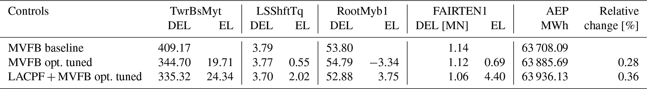
Table 5 summarizes the DEL, EL, and AEP of the three controls. Here, it is assumed that the lifetime fatigue loads only result from DLC 1.2. Note that the EL and the relative change are both calculated relative to the baseline MVFB control. In comparison with the baseline control, with the optimally tuned MVFB control, the DEL of the tower is obviously reduced, leading to an extended lifetime of 19.7 years. In addition, the loads on the shaft and fairlead are slightly reduced. However, the blade root load is clearly increased; therefore, the lifetime is reduced by 3.3 years. In terms of the AEP, there is a slight increment of about 0.28 %. Introducing feedforward control supported by lidar further improves the overall control performance. With the LACPF + MVFB control, the further reduction in the tower base load corresponds to a lifetime extension of 4.6 years. Also, the shaft and blade root loads are reduced slightly. As a consequence, the negative impact of the optimally tuned MVFB control on the blade root load is avoided. The AEP increment under the LACPF + MVFB control is also slightly higher than that under the MVFB-only control. Furthermore, using the LACPF control results in a clear load reduction in the fairlead of the mooring system.
This paper assesses lidar-assisted collective pitch feedforward (LACPF) and multivariable feedback (MVFB) controls for the IEA 15.0 MW reference turbine. The main contributions of this work include the following: (a) optimizing a four-beam pulsed lidar for controlling a large floating turbine, (b) optimal tuning of speed regulation gains and platform feedback gains for the MVFB and LACPF + MVFB controls; and (c) assessing the benefits of the two control strategies using realistic offshore turbulence spectral characteristics.
The IEC 61400-3 (2009) standard for offshore turbine design does not specify turbulence spectral parameters for offshore conditions. The typical parameter listed in IEC 61400-1 (2019) tends to underestimate the occurrence of large-scale coherent turbulent eddies. In the time domain, these eddies are reflected as low-frequency and spatially correlated turbulence. We define realistic turbulence parameters representative of an offshore site based on the literature, which are further used for load and extreme-value assessments.
A four-beam, single-range pulsed lidar is optimized for control. For the large-rotor floating turbine, it is found that a lidar focusing on a further distance can estimate the rotor-effective wind speed better. A notch filter is necessary for floating turbines to avoid conflict between the LACPF control and the MVFB control. Because of the notch filter, additional time delays are introduced by the filtering. A further focusing distance for the lidar system helps to avoid the LACPF command reacting too late.
The speed-regulating proportional–integral controls are re-tuned, aiming to minimize the tower loads and to avoid overspeed. When tuning with LACPF, the optimal values for the proportional gains are found to be lower than those tuned without LACPF. In very high wind speed ranges, the tuning results with or without LACPF are similar. The optimal integral time constants are found to be generally similar, whether considering LACPF or not. The floating feedback gains are also optimized. The optimal values are found to be close to the valley where the blade pitch rates are the lowest. After the valley, increasing the floating feedback gains has marginal reductions in tower load but amplifies the blade pitch actions significantly.
The control performances of the optimally tuned controls are assessed and compared with those of a baseline control provided by NREL's Reference OpenSource Controller toolbox. It is observed that the re-tuning of the gains clearly reduces the maximum generator speed, while with the optimally tuned MVFB control, there are still some overshoots of the generator speed that are higher than the selected threshold (125 % of the rated speed) when the mean wind speed is higher than 20 m s−1. The overspeed is not present in the simulation results using the LACPF + MVFB control. Significant reductions in the maximum values of the blade tip deflection and platform pitch are observed using the optimally tuned MVFB and LACPF + MVFB controls as well. In terms of the fatigue load resulting from DLC 1.2, the most significant improvement from re-tuning the feedback loops with the MVFB control is the extension of the tower lifetimes by 19.7 years. If a lidar-assisted control system is deployed, the tower lifetime can be extended by 24.3 years, and the fairlead lifetime can be 4.4 years longer. There are also extensions of shaft and blade lifetimes of 2.0 and 3.8 years, respectively.
For both MVFB and LACPF + MVFB controls, there is clearly an increase in blade pitch activities at very high wind speeds, which can potentially cause more damage to the gear and bearing of the pitch actuator. For the LACPF + MVFB control, there are decrements in the pitch activities close to the rated wind speed. Because the mean wind speed has a higher probability here, it could be possible that the LACPF + MVFB control overall does not cause more damage to the pitch actuator. However, a more detailed assessment can be made by more complete modeling of the pitch actuator damage. In addition, the fatigue analysis of the mooring system can be further extended. The potential of LACPF to reduce the load in mooring systems can further be explored by other feedforward control strategies.
An example time series of the OpenFAST simulations is shown in Fig. A1. For the three control configurations, the results are simulated using the turbulence fields generated by the identical random seed. Figure A1a shows the raw line-of-sight measurement provided by the LidarSim module. The measurements are performed at different beam directions; therefore, there are considerable high-frequency fluctuations caused by the uncorrelated high-frequency components in the turbulence field. The missing and unconnected points are unavailable line-of-sight measurements due to blade blockage. Figure A1b shows the lidar-estimated and filtered REWS, which is the coherent low-frequency component in the turbulence.
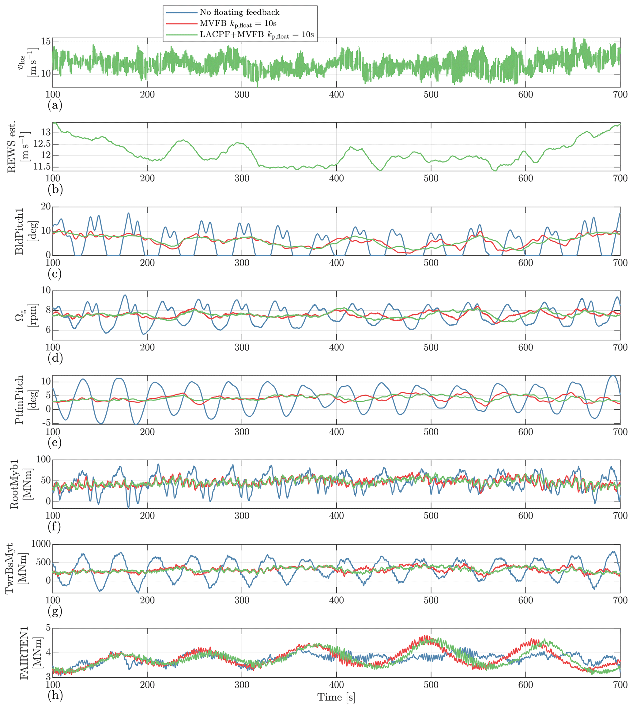
Figure A1Example time series of the OpenFAST simulations, simulated with a mean wind speed of 12 m s−1.
OpenFAST version 3.0 with an integrated lidar simulator can be accessed via https://doi.org/10.5281/zenodo.7594971 (fengguoFUAS, 2023a). The 4D Mann turbulence generator can be found at https://doi.org/10.5281/zenodo.7594951 (fengguoFUAS, 2023b). The source codes of the wrapper DLL, baseline lidar data processing DLL, pitch feedforward DLL, and modified ROSCO DLL are all available from https://doi.org/10.5281/zenodo.7594961 (fengguoFUAS, 2023c).
The turbine data used for this research are available from https://doi.org/10.5281/zenodo.8070464 (Barter et al., 2023). Simulation data of this paper are available upon request from the corresponding author.
FG conceived the concept, performed the simulations, and prepared the paper. DS provided support with respect to the verifification of the simulation results, contributed to editing, and provided general guidance.
The contact author has declared that neither of the authors has any competing interests.
Publisher’s note: Copernicus Publications remains neutral with regard to jurisdictional claims in published maps and institutional affiliations.
This research has been supported by the European Union’s Horizon 2020 research and innovation program under the Marie Skłodowska-Curie grant with agreement no. 858358 (LIKE – Lidar Knowledge Europe).
This paper was edited by Irene Eguinoa and reviewed by two anonymous referees.
Abbas, N. J., Zalkind, D. S., Pao, L., and Wright, A.: A reference open-source controller for fixed and floating offshore wind turbines, Wind Energ. Sci., 7, 53–73, https://doi.org/10.5194/wes-7-53-2022, 2022. a, b, c, d, e, f
Allen, C., Viscelli, A., Dagher, H., Goupee, A., Gaertner, E., Abbas, N., Hall, M., and Barter, G.: Definition of the UMaine VolturnUS-S Reference Platform Developed for the IEA Wind 15-Megawatt Offshore Reference Wind Turbine, Tech. Rep. NREL/TP-5000-76773, NREL, https://doi.org/10.2172/1660012, 2020. a, b
Bachynski, E. E. and Eliassen, L.: The effects of coherent structures on the global response of floating offshore wind turbines, Wind Energy, 22, 219–238, https://doi.org/10.1002/we.2280, 2019. a, b, c, d, e, f
Barrera, C., Battistella, T., Guanche, R., and Losada, I. J.: Mooring system fatigue analysis of a floating offshore wind turbine, Ocean Eng., 195, 106670, https://doi.org/10.1016/j.oceaneng.2019.106670, 2020. a
Barter, G., Bortolotti, P., Gaertner, E., Abbas, N. J., dzalkind, Rinker, J., Zahle, F., T-Wainwright, Branlard, E., Wang, L., Padrón, L. A., and Hall, M.: IEAWindTask37/IEA-15-240-RWT: v1.1.6: HAWC2 monopile, VolturnUS-S CAD model, Zenodo [data set], https://doi.org/10.5281/zenodo.8070464, 2023.
Bossanyi, E. A., Kumar, A., and Hugues-Salas, O.: Wind turbine control applications of turbine-mounted LIDAR, J. Phys. Conf. Ser., 555, 012011, https://doi.org/10.1088/1742-6596/555/1/012011, 2014. a
Bredmose, H., Lemmer, F., Borg, M., Pegalajar-Jurado, A., Mikkelsen, R., Larsen, T. S., Fjelstrup, T., Yu, W., Lomholt, A., Boehm, L., and Armendariz, J. A.: The Triple Spar campaign: Model tests of a 10MW floating wind turbine with waves, wind and pitch control, Enrgy. Proced., 137, 58–76, https://doi.org/10.1016/j.egypro.2017.10.334, 2017. a
Catapult, O.: Floating Offshore Wind: Cost Reduction Pathways to Subsidy Free, Tech. rep., Catapult, Offshore Renewable Energy, https://ore.catapult.org.uk/wp-content/uploads/2021/01/FOW-Cost-Reduction-Pathways-to-Subsidy-Free-report-.pdf (last access: 12 August 2023), 2021. a
Cheynet, E., Jakobsen, J. B., and Obhrai, C.: Spectral characteristics of surface-layer turbulence in the North Sea, Enrgy. Proced., 137, 414–427, https://doi.org/10.1016/j.egypro.2017.10.366, 2017. a
Cheynet, E., Jakobsen, J. B., and Reuder, J.: Velocity spectra and coherence estimates in the marine atmospheric boundary layer, Bound.-Lay. Meteorol., 169, 429–460, https://doi.org/10.1007/s10546-018-0382-2, 2018. a, b, c, d, e
de Maré, M. and Mann, J.: Validation of the Mann spectral tensor for offshore wind conditions at different atmospheric stabilities, J. Phys. Conf. Ser., 524, 012106, https://doi.org/10.1088/1742-6596/524/1/012106, 2014. a
DNV-GL: Bladed theory manual: version 4.8, Tech. rep., Garrad Hassan & Partners Ltd., Bristol, UK, 2016. a
Fleming, P. A., Peiffer, A., and Schlipf, D.: Wind turbine controller to mitigate structural loads on a floating wind turbine platform, J. Offshore Mech. Arct., 141, 061901, https://doi.org/10.1115/1.4042938, 2019. a, b
Gaertner, E., Rinker, J., Sethuraman, L., Zahle, F., Anderson, B., Barter, G. E., Abbas, N. J., Meng, F., Bortolotti, P., Skrzypinski, W., Scott, G. N., Feil, R., Bredmose, H., Dykes, K., Shields, M., Allen, C., and Viselli, A.: IEA Wind TCP Task 37: Definition of the IEA 15-Megawatt Offshore Reference Wind Turbine, Technical Report, https://doi.org/10.2172/1603478, 2020. a, b
Guo, F., Mann, J., Peña, A., Schlipf, D., and Cheng, P. W.: The space-time structure of turbulence for lidar-assisted wind turbine control, Renew. Energ., 195, 293–310, https://doi.org/10.1016/j.renene.2022.05.133, 2022a. a, b, c, d
Guo, F., Schlipf, D., Zhu, H., Platt, A., Cheng, P. W., and Thomas, F.: Updates on the OpenFAST Lidar Simulator, J. Phys. Conf. Ser., 2265, 042030, https://doi.org/10.1088/1742-6596/2265/4/042030, 2022b. a
Guo, F., Schlipf, D., and Cheng, P. W.: Evaluation of lidar-assisted wind turbine control under various turbulence characteristics, Wind Energ. Sci., 8, 149–171, https://doi.org/10.5194/wes-8-149-2023, 2023. a, b, c, d, e, f, g, h, i, j, k, l, m, n
Held, D. P. and Mann, J.: Lidar estimation of rotor-effective wind speed – an experimental comparison, Wind Energ. Sci., 4, 421–438, https://doi.org/10.5194/wes-4-421-2019, 2019. a
IEC 61400-1: Wind energy generation systems – Part 1: Design requirements, 2019. a, b, c, d, e, f, g, h
IEC 61400-3: Wind turbines – Part 3: Design requirements for offshore wind turbines, 2009. a, b, c
IEC 61400-3-2: Wind energy generation systems – Part 3-2: Design requirements for floating offshore wind turbines, 2019. a
fengguoFUAS: MSCA-LIKE/OpenFAST3.0_Lidarsim: Open-FAST3.0_Lidarsim (OpenFAST3.0_Lidarsim_v1), Zenodo [code], https://doi.org/10.5281/zenodo.7594971, 2023a.
fengguoFUAS: MSCA-LIKE/4D-Mann-Turbulence-Generator: 4D-Mann-Turbulence-Generator (4D_MannTurbulence_v1), Zenodo [code], https://doi.org/10.5281/zenodo.7594951, 2023b.
fengguoFUAS: MSCA-LIKE/Baseline-Lidar-assisted-Controller: Baseline-Lidar-assisted-Controller (Baseline-Lidar-assisted-Controllerv_1), Zenodo [code], https://doi.org/10.5281/zenodo.7594961, 2023c.
Jonkman, J.: Influence of Control on the Pitch Damping of a Floating Wind Turbine, 46th AIAA Aerospace Sciences Meeting and Exhibit, Reno, Nevada, 7–10 January 2008, https://doi.org/10.2514/6.2008-1306, 2008. a
Knight, J. M. and Obhrai, C.: The influence of an unstable turbulent wind spectrum on the loads and motions on floating Offshore Wind Turbines, IOP C. Ser. Mat. Sci., 700, 012005, https://doi.org/10.1088/1757-899X/700/1/012005, 2019. a
Lemmer, F.: Low-order modeling, controller design and optimization of floating offshore wind turbines, PhD thesis, Unversity of Stuttgart, 2018. a
Lemmer, F., Müller, K., Yu, W., Schlipf, D., and Cheng, P. W.: Optimization of floating offshore wind turbine platforms with a self-tuning controller, in: International Conference on Ocean, Offshore and Arctic Engineering, Trondheim, Norway, 25–30 June 2017, https://doi.org/10.1115/omae2017-62038, 2017. a
Lemmer, F., Yu, W., Schlipf, D., and Cheng, P. W.: Robust gain scheduling baseline controller for floating offshore wind turbines, Wind Energy, 23, 17–30, https://doi.org/10.1002/we.2408, 2020. a, b, c
Li, L., Gao, Z., and Moan, T.: Joint environmental data at five european offshore sites for design of combined wind and wave energy devices, in: International Conference on Offshore Mechanics and Arctic Engineering, Nantes, France, 9–14 June 2013, https://doi.org/10.1115/OMAE2013-10156, 2013. a, b
Lio, W. H., Meng, F., and Larsen, G. C.: On LiDAR-assisted wind turbine retrofit control and fatigue load reductions, J. Phys. Conf. Ser., 2265, 032072, https://doi.org/10.1088/1742-6596/2265/3/032072, 2022. a
Mann, J.: The spatial structure of neutral atmospheric surface-layer turbulence, J. Fluid Mech., 273, 141–168, 1994. a
Mann, J.: Wind field simulation, Probabilist. Eng. Mech., 13, 269–282, 1998. a
Matsuishi, M. and Endo, T.: Fatigue of metals subjected to varying stress, Japan Society of Mechanical Engineers, Fukuoka, Japan, 68, 37–40, 1968. a
Meng, F., Lio, W. H., and Larsen, G. C.: Wind turbine LIDAR-assisted control: Power improvement, wind coherence and loads reduction, J. Phys. Conf. Ser., 2265, 022060, https://doi.org/10.1088/1742-6596/2265/2/022060, 2022. a
Mirzaei, M. and Mann, J.: Lidar configurations for wind turbine control, J. Phys. Conf. Ser., 753, 032019, https://doi.org/10.1088/1742-6596/753/3/032019, 2016. a
NREL: ROSCO, Version 2.6.0, https://github.com/NREL/ROSCO (last access: 12 August 2023), 2021. a, b, c
Nybø, A., Nielsen, F. G., Reuder, J., Churchfield, M. J., and Godvik, M.: Evaluation of different wind fields for the investigation of the dynamic response of offshore wind turbines, Wind Energy, 23, 1810–1830, https://doi.org/10.1002/we.2518, 2020. a
Obukhov, A.: Turbulence in an atmosphere with a non-uniform temperature, Bound.-Lay. Meteorol., 2, 7–29, https://doi.org/10.1007/BF00718085, 1971. a
Peña, A.: Østerild: A natural laboratory for atmospheric turbulence, J. Renew. Sustain. Ener., 11, 063302, https://doi.org/10.1063/1.5121486, 2019. a
Putri, R. M., Cheynet, E., Obhrai, C., and Jakobsen, J. B.: Turbulence in a coastal environment: the case of Vindeby, Wind Energ. Sci., 7, 1693–1710, https://doi.org/10.5194/wes-7-1693-2022, 2022. a
Rivera-Arreba, I., Wise, A. S., Hermile, M., Chow, F. K., and Bachynski-Polić, E. E.: Effects of atmospheric stability on the structural response of a 12 MW semisubmersible floating wind turbine, Wind Energy, 25, 1917–1937, https://doi.org/10.1002/we.2775, 2022. a
Russell, A. J., Collu, M., McDonald, A., Thies, P. R., Mortimer, A., and Quayle, A. R.: Review of LIDAR-assisted Control for Offshore Wind Turbine Applications, J. Phys. Conf. Ser., 2362, 012035, https://doi.org/10.1088/1742-6596/2362/1/012035, 2022. a
Sandner, F., Schlipf, D., Matha, D., and Cheng, P. W.: Integrated Optimization of Floating Wind Turbine Systems, Ocean Renewable Energy of International Conference on Offshore Mechanics and Arctic Engineering, San Francisco, California, USA, 8–13 June 2014, https://doi.org/10.1115/OMAE2014-24244, 2014. a
Schlipf, D.: Lidar-Assisted Control Concepts for Wind Turbines, Ph.D. thesis, University of Stuttgart, https://doi.org/10.18419/opus-8796, 2015. a, b, c, d, e, f, g
Schlipf, D., Simley, E., Lemmer, F., Pao, L., and Cheng, P. W.: Collective pitch feedforward control of floating wind turbines using Lidar, Journal of Ocean and Wind Energy, 2, 223–230, https://doi.org/10.17736/jowe.2015.arr04, 2015. a
Schlipf, D., Fürst, H., Raach, S., and Haizmann, F.: Systems engineering for lidar-assisted control: a sequential approach, J. Phys. Conf. Ser., 1102, 012014, https://doi.org/10.1088/1742-6596/1102/1/012014, 2018. a
Schlipf, D., Lemmer, F., and Raach, S.: Multi-Variable Feedforward Control for Floating Wind Turbines Using Lidar, in: International Ocean and Polar Engineering Conference, Shanghai, China, 11–16 October 2020, https://doi.org/10.18419/opus-11067, 2020. a, b
Simley, E. and Pao, L. Y.: Reducing LIDAR wind speed measurement error with optimal filtering, in: Proceedings of the American Control Conference, Washington, DC, USA, 17–19 June 2013, https://doi.org/10.1109/ACC.2013.6579906, 2013. a
Simley, E., Fürst, H., Haizmann, F., and Schlipf, D.: Optimizing lidars for wind turbine control applications results from the IEA wind task 32 workshop, Remote Sens., 10, 863, https://doi.org/10.3390/rs10060863, 2018. a
Simley, E., Bortolotti, P., Scholbrock, A., Schlipf, D., and Dykes, K.: IEA Wind Task 32 and Task 37: Optimizing Wind Turbines with Lidar-Assisted Control Using Systems Engineering, J. Phys. Conf. Ser., 1618, 042029, https://doi.org/10.1088/1742-6596/1618/4/042029, 2020. a, b
Somoano, M., Battistella, T., Rodríguez-Luis, A., Fernández-Ruano, S., and Guanche, R.: Influence of turbulence models on the dynamic response of a semi-submersible floating offshore wind platform, Ocean Eng., 237, 109629, https://doi.org/10.1016/j.oceaneng.2021.109629, 2021. a
Taylor, G. I.: The spectrum of turbulence, P. Roy. Soc. Lond. A Mat., 164, 476–490, https://doi.org/10.1098/rspa.1938.0032, 1938. a
van der Veen, G., Couchman, I., and Bowyer, R.: Control of floating wind turbines, in: Proceedings of the American Control Conference, Montreal, Canada, 27–29 June 2012, https://doi.org/10.1109/ACC.2012.6315120, 2012. a
Ward, D., Collu, M., and Sumner, J.: Reducing Tower Fatigue through Blade Back Twist and Active Pitch-to-Stall Control Strategy for a Semi-Submersible Floating Offshore Wind Turbine, Energies, 12, 1897, https://doi.org/10.3390/en12101897, 2019. a
Wu, J. and Kim, M.-H.: Generic Upscaling Methodology of a Floating Offshore Wind Turbine, Energies, 14, 8490, https://doi.org/10.3390/en14248490, 2021. a
Zalkind, D., Abbas, N. J., Jasa, J., Wright, A., and Fleming, P.: Floating wind turbine control optimization, J. Phys. Conf. Ser., 2265, 042021, https://doi.org/10.1088/1742-6596/2265/4/042021, 2022. a, b, c, d, e
FINO1 is an offshore research platform located in the North Sea at a water depth close to 30 m: https://www.fino1.de/de/standort.html (last access: 8 August 2023).
The 4D Mann turbulence generator is accessible from https://github.com/MSCA-LIKE/4D-Mann-Turbulence-Generator (last access: 8 August 2023).