the Creative Commons Attribution 4.0 License.
the Creative Commons Attribution 4.0 License.
 | 09 Feb 2023
Evaluation of lidar-assisted wind turbine control under various turbulence characteristics
David Schlipf
Po Wen Cheng
Lidar systems installed on the nacelle of wind turbines can provide a preview of incoming turbulent wind. Lidar-assisted control (LAC) allows the turbine controller to react to changes in the wind before they affect the wind turbine. Currently, the most proven LAC technique is the collective pitch feedforward control, which has been found to be beneficial for load reduction. In literature, the benefits were mainly investigated using standard turbulence parameters suggested by the IEC 61400-1 standard and assuming Taylor's frozen hypothesis (the turbulence measured by the lidar propagates unchanged to the rotor). In reality, the turbulence spectrum and the spatial coherence change by the atmospheric stability conditions. Also, Taylor's frozen hypothesis does not take into account the coherence decay of turbulence in the longitudinal direction. In this work, we consider three atmospheric stability classes, unstable, neutral, and stable, and generate four-dimensional stochastic turbulence fields based on two models: the Mann model and the Kaimal model. The generated four-dimensional stochastic turbulence fields include realistic longitudinal coherence, thus avoiding assuming Taylor's frozen hypothesis. The Reference Open-Source Controller (ROSCO) by NREL is used as the baseline feedback-only controller. A reference lidar-assisted controller is developed and used to evaluate the benefit of LAC. Considering the NREL 5.0 MW reference wind turbine and a typical four-beam pulsed lidar system, it is found that the filter design of the LAC is not sensitive to the turbulence characteristics representative of the investigated atmospheric stability classes. The benefits of LAC are analyzed using the aeroelastic tool OpenFAST. According to the simulations, LAC's benefits are mainly the reductions in rotor speed variation (up to 40 %), tower fore–aft bending moment (up to 16.7 %), and power variation (up to 20 %). This work reveals that the benefits of LAC can depend on the turbulence models, the turbulence parameters, and the mean wind speed.
- Article
(9955 KB) - Full-text XML
- BibTeX
- EndNote


Traditionally, wind turbine control only relies on the feedback (FB) control strategy. For the above-rated wind operations, the generator speed change caused by the turbulence wind is measured, and the blade pitch is adjusted to maintain the rated rotor/generator speed. This means that the turbine reacts to the wind disturbance only after it has been affected. A nacelle lidar scanning in front of the turbine can provide a preview of the incoming turbulence. Based on the preview, a rotor-effective wind speed (REWS) can be derived and used to provide a feedforward pitch signal. The feedforward pitch signal can be simply added to the conventional feedback controller (Schlipf, 2015), which is often referred to as lidar-assisted collective pitch feedforward control (CPFF). Apart from CPFF, there are other lidar-assisted control (LAC) concepts that have been presented in the literature, e.g., the works by Schlipf et al. (2013b), Schlipf (2015), Schlipf et al. (2020). However, CPFF is so far the most promising technology, and it has been deployed in commercial projects (Schlipf et al., 2018b). Thus, we focus on assessing the benefits of CPFF in this work.
To utilize the lidar measurement for LAC, a correlation study is necessary to determine how much the lidar-estimated REWS is correlated with the actual REWS that acts on the turbine rotor. Some facts that could have an impact on the measurement correlation are listed below:
- a.
Lidar measurement positions. A typical lidar system has fewer measurement points within the rotor-swept area compared to the rotational sampling rotor. Thus, the lidar-estimated REWS is less spatially filtered.
- b.
Line-of-sight (LOS) wind speed vlos measurement. This is the cumulative projection of longitudinal (u), lateral (v), and vertical (w) components in the lidar beam direction. The turbine's aerodynamic performance is mainly driven by the u component, and lidar is expected to measure the u component for control purposes. In reality, the lidar measurements can be contaminated by lateral and vertical wind speed components (Held and Mann, 2019), because of the beam opening angles, the nacelle movement, or the turbine yaw misalignment.
- c.
Lidar probe volume. The lidar measurement is the weighted average of the LOS along the lidar beam (Peña et al., 2013, 2017).
- d.
Turbulence spectrum and coherence. The lidar measurement coherence is mathematically derived based on the spectrum and coherence (Schlipf, 2015; Held and Mann, 2019; Guo et al., 2022a), which will be further discussed in Sect. 3.
- e.
Atmospheric stability. The turbulence spectrum and coherence have been shown to vary by atmospheric stability conditions (Peña, 2019; Guo et al., 2022a).
According to the IEC standard, two turbulence models are commonly used for wind turbine design as provided by the IEC 61400-1:2019 (2019) standard; one is the Mann (1994) uniform shear model, and another one is the Kaimal et al. (1972) spectra combined with exponential coherence model (hereafter referred to as the Mann model and the Kaimal model, respectively). The derivation of lidar measurement coherence based on a specific turbulence model has been studied in the literature. For example, Schlipf et al. (2013a) and Schlipf (2015) show the derivation by the Kaimal model. Mirzaei and Mann (2016), Held and Mann (2019), and Guo et al. (2022a) demonstrate the solution for the Mann model. Based on the two turbulence models, several authors investigated the lidar measurement coherence considering different lidar measurement trajectories and turbine sizes, e.g., the works by Simley et al. (2018), Held and Mann (2019), and Dong et al. (2021). Specifically, in work by Dong et al. (2021), the lidar measurement coherence by the two turbulence models is compared, assuming Taylor’s frozen hypothesis. In this paper, we also consider two turbulence models and include turbulence evolution in our analysis.
Once the lidar measurement coherence is analyzed, a filter needs to be designed to filter out uncorrelated information in the lidar-estimated REWS. Because the filter introduces a certain time delay (Schlipf, 2015), a timing algorithm is necessary to ensure the turbine feedforward pitch acts at the correct time. Usually, the time that turbulence requires to propagate from upstream to downstream, the time delay in the pitch actuator, the time delay by averaging sequential lidar measurements of a full scan, and the time delay caused by filtering should all be considered. In this work, we will contribute by providing a reference lidar-assisted controller. It includes (1) a lidar data processing module that provides the lidar-estimated REWS, (2) a feedforward blade pitch rate provider, and (3) a modified Reference Open-Source Controller (ROSCO) with the capability to accept feedforward pitch rate signal. ROSCO (Abbas et al., 2022) is an open, modular, and fully adaptable baseline wind turbine controller with industry-standard functionality.
When evaluating the benefits of LAC, Schlipf (2015) uses the Kaimal model with the turbulence spectral parameters provided by the IEC standard through FAST (Jonkman and Buhl, 2005) (the previous version of OpenFAST NREL, 2022) aeroelastic simulation. With a circular scanning lidar, LAC is found to bring a noticeable reduction in the lifetime damage equivalent load (DEL) in the tower base fore–aft bending moment, the low-speed shaft torque, and the blade root out-of-plane moment. However, the variations of turbulence parameters have not been considered.
The recent developments in turbulence simulation tools, evoTurb by Chen et al. (2022) and the 4D Mann Turbulence Generator by Guo et al. (2022a), have made it possible to integrate turbulence evolution into aeroelastic simulation. With the updated OpenFAST lidar simulator (Guo et al., 2022b), the 4D turbulence field can be imported into OpenFAST, and the upstream lidar measurement can be simulated using the upstream turbulence fields.
The variation of turbulence parameters from the standard values given by IEC 61400-1:2019 (2019) can be interesting for wind energy. Turbulence parameters under different atmospheric stability classes are investigated and summarized by, e.g., Cheynet et al. (2017), Peña (2019), and Nybø et al. (2020). For example, Fig. 1 shows how the turbulence structure changes by the turbulence length scale L. A larger coherent eddy structure is observed in the unstable stability, and the eddy structure is much smaller in size under the stable stability. In the neutral case, the eddy structure is somewhere between the two cases. The length scale can have an impact on the power spectrum and turbulence spatial coherence (as later discussed in Sect. 2.4). Further, the spectrum and coherence can have potential impacts not only on the lidar measurement coherence but also on the turbine loads because the turbulence spectrum peaks can distribute at different frequency ranges, and different frequencies can produce different excitations for the turbine structure motions.
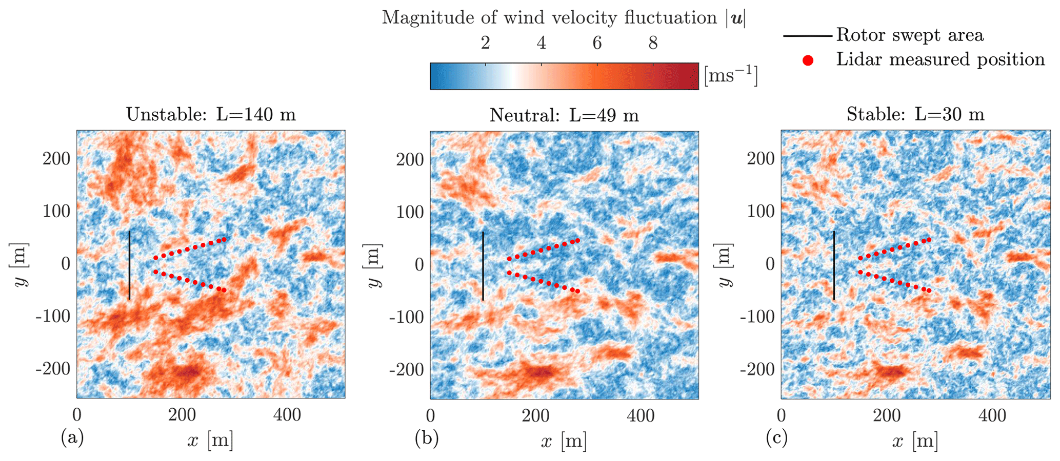
Figure 1Top view of a turbulence field showing the eddy structures under different atmospheric stability, simulated using the 4D Mann Turbulence Generator with parameters listed in Table 1. The lidar measured positions are plotted based on a typical four-beam pulsed lidar. The rotor-swept area is drawn based on the NREL 5.0 MW reference wind turbine which has a rotor diameter of 126 m. The length scales L are chosen based on studies by Peña (2019) and Guo et al. (2022a).
In this work, we summarize how the turbulence spectrum and spatial coherence can vary by atmospheric stability from literature. Three atmospheric stability classes, unstable, neutral, and stable, are considered. For each atmospheric stability class, the Mann model parameters are collected, and then the Kaimal model parameters are fitted to have similar spectra and coherence compared to the Mann model. Then the four-dimensional stochastic turbulence fields are generated using the 4D Mann Turbulence Generator (Guo et al., 2022a) and evoTurb (Chen et al., 2022). The benefits of LAC are then assessed using a typical four-beam commercial lidar configuration and the 5 MW reference wind turbine by NREL (Jonkman et al., 2009) through the lidar simulator-integrated aeroelastic simulation tool: OpenFAST. To compare CPFF with the traditional feedback-only controller, ROSCO is considered to be the baseline feedback controller.
This paper is organized as follows: Sect. 2 gives the background about turbulence modeling, Sect. 3 discusses the correlation between the REWS and the lidar-estimated REWS, Sect. 4 introduces the design of lidar-assisted controller, Sect. 5 presents and discusses the simulation results, and Sect. 6 draws conclusions for this research.
In this section, we first introduce the Mann (1994) model and the Kaimal et al. (1972) spectrum and exponential coherence model (Davenport, 1961) used in this work. Then, the methods to include turbulence evolution in the two turbulence models are discussed. Lastly, we show the turbulence spectra and coherence under different atmospheric stability classes.
2.1 The Mann turbulence model
The Mann (1994) model is a spectral tensor model recommended by the IEC 61400-1:2019 (2019) standard for wind turbine load calculations. It applies the rapid distortion theory (Hunt and Carruthers, 1990) to an isotropic spectral tensor based on the von Kármán (1948) energy spectrum, to model the shear stretched eddy structures.
At a certain moment, the velocity field can be described by , with the position vector in space (Cartesian coordinate). After applying Taylor's frozen hypothesis (Taylor, 1938) and Reynolds' decomposition, the fluctuation part of the turbulence about the mean flow is assumed homogeneous in space, and it can be computed from the Fourier transform
where is the Fourier coefficient of the velocity field, i is the imaginary unit, and means the integration over all the wavenumber vectors . Conversely,
with . The Fourier coefficients are connected to the elements in the spectral tensor (denoted as Φ) by
where 〈 〉 means the ensemble average, * denotes the complex conjugate, and δ() is the Dirac delta function. k′ is also the wavenumber vectors, and it is used to differentiate with k. Equation (3) implies that the ensemble averages of the Fourier coefficients of non-identical wavenumber vectors are all zero. are indexes that stand for u, v, and w components, i.e., . The detailed expression of Φij(k) can be found from the work by Mann (1994). Note that the spectral tensor Φ is a 3 by 3 matrix for any wavenumber vector k, and Φij(k) denotes an element in the matrix. Except for the wavenumber vector, there are three other parameters in the model. They are as follows:
-
[] is an energy level constant valid in the inertial subrange, composed by the spectral Kolmogorov constant α and the rate of viscous dissipation of specific turbulent kinetic energy ε (Mann, 1998). This constant actually acts as a proportional gain to the spectral tensor and it is often adjusted to obtain a specific turbulence intensity (TI).
-
L [m] is a length scale related to the size of the eddies containing the most energy (Held and Mann, 2019).
-
Γ [–] is a non-dimensional anisotropy due to shear effect in near-surface boundary layer. When Γ=0, the turbulence is isotropic (Mann, 1994, 1998).
Mann (1994) uses Γ to calculate the eddy lifetime by
where 2F1() is a hypergeometric function and is the mean vertical shear profile. The eddy lifetime τ actually distorts the wavenumber k3 (corresponds to the z direction) from the initial shearless state k30 by . Here, is a non-dimensional distortion factor (Mann, 1994). The effect of the hypergeometric function 2F1() is to have
where b1 and b2 are two constants standing for the slopes of τ in logarithmic scale. Instead of using the hypergeometric function, Guo et al. (2022a) proposed another equation for the eddy lifetime
which is straightforward to adjust the slopes of the eddy lifetime. They found that adjusting the slope constant b1 for stable atmospheric stability tends to give better agreements of spectra and coherence between the model and the measurements from a lidar and a meteorological mast. We will use Eq. (6) for the rest of this paper.
The one-dimensional (along the longitudinal wavenumber) cross-spectra of all velocity components with separations Δy and Δz can be obtained by
where . Specifically, when i=j and , it becomes the auto-spectrum of one velocity component at one point, usually written as Fii(k1). The magnitude-squared coherence between two points in the same yz plane is often interesting, which can be calculated by (Mann, 1994)
And the yz plane co-coherence and quad-coherence are defined by
and
where ℜ and ℑ are the real and imaginary number operators, respectively.
2.2 Kaimal spectra and exponential coherence model
The Kaimal model given by IEC 61400-1:2019 (2019) uses the following formula to determine the auto-spectra of velocity components:
where f is the frequency, Li is the integral length scale, σi is the standard deviation, and Uref is the reference wind speed equivalent to hub-height mean wind speed. The coherence (with square) of the u components of two points in the yz plane is described as
with the separation distance, ayz the coherence decay constant, and Lc the coherence scale parameter. Note that the coherence without square is used in IEC 61400-1:2019 (2019). The yz plane coherence for the v and w components is not given by the IEC 61400-1:2019 (2019), and they are ignored in this work.
2.3 Modeling of turbulence evolution
The turbulence evolution refers to the phenomenon that the eddy structure changes when the turbulence propagates from upstream to downstream. It is often represented using longitudinal coherence.
2.3.1 Extending the Mann model to include evolution
A space–time tensor that extends the three-dimensional Mann spectral tensor Φ to count for the temporal evolution of the turbulence field has been proposed by Guo et al. (2022a). The space–time tensor is evaluated to provide good agreements on the turbulence spectra and coherence including the spectra of all velocity components and the coherence with longitudinal, vertical–lateral, and all combined spatial separations. The validation has been made using measurement from a pulsed lidar and a meteorological mast. Details of the model validation can be found in the work by Guo et al. (2022a). The space–time tensor is written as
which defines the ensemble average
where denotes the Fourier coefficients of the turbulence field at time t0+Δt. τe is another eddy lifetime (different from τ) that defines the temporal evolution of the turbulence field. The expression
was found to predicts the longitudinal coherence well as investigated by Guo et al. (2022a). Here, γ is a parameter that determines the strength of turbulence evolution.
In the space–time tensor, the turbulence field is assumed to travel with a mean reference wind speed Uref. After time Δt, the field moves downstream in the positive x direction by UrefΔt. Thus, for two points with a longitudinal separation of Δx, the longitudinal coherence (magnitude-squared) of u component can be calculated from
where
is the auto-spectrum of u component. In practice, the wavenumber-based spectra or coherence is converted to the frequency-based ones using conversion , assuming Taylor (1938)'s frozen hypothesis.
2.3.2 Exponential longitudinal coherence model
On the other hand, Simley and Pao (2015) adjusted the exponential coherence model listed in the IEC 61400-1:2019 (2019) by replacing the transverse and vertical separations with longitudinal separations, which gives the following expression for the longitudinal coherence
where ax and bx are two parameters, and f is the frequency. Specifically, ax determines the decay effect of the coherence, and bx determines the intercept (value at 0 frequency) (Chen et al., 2021). Simley and Pao (2015) validated Eq. (19) using large eddy simulations (LESs) of different atmospheric stability classes. Besides, Davoust and von Terzi (2016) and Chen et al. (2021) verified the exponential evolution model using lidar measurement, showing that the expression by Simley and Pao (2015) agrees well with the measurement. In their study, they found possible ax and bx by fitting the coherence calculated from measurement data to the model. As a result, was observed, and bx was found in the order of magnitude .
To include the exponential longitudinal coherence model into the analysis of lidar measurement correlation, a general “direct product” approach is used to combine the lateral-vertical coherence and the longitudinal coherence (Laks et al., 2013; Simley, 2015; Bossanyi et al., 2014; Schlipf et al., 2013a), which means the overall coherence
As shown by Chen et al. (2022), the direct product approach allows an efficient algorithm to generate the Kaimal-model-based 4D stochastic turbulence field using statically independent 3D turbulence fields using evoTurb.
2.4 Turbulence under different atmospheric stability classes
Atmospheric stability indicates the buoyancy effect on the turbulence generation, and it is usually related to the temperature gradient by height. It is interesting to investigate its impact on the filter design of LAC since the turbine will experience different atmospheric stability conditions during operation. The filter is necessary to filter out the uncorrelated frequencies in the REWS estimated by lidar, as will be discussed later in Sect. 3. In the rest of this paper, we use the Mann turbulence parameter sets representative of unstable, neutral, and stable conditions based on the study by Peña (2019) and Guo et al. (2022a), as listed in Table 1. It is worth mentioning that the parameter is scaled such that the TI corresponds to the IEC 61400-1:2019 (2019) class 1A definition. Actually, the turbulence intensity is related to the atmospheric conditions. Usually, TI is generally high in unstable stability, moderate in neutral stability, and low in stable stability (Peña et al., 2017). In this work, we emphasize analyzing the impact of turbulence length scale and anisotropy on turbine loads and LAC benefits. Therefore, the same TI level is assumed for the three stability classes. This assumption tends to be not realistic, but it helps to identify the impact of length scale on turbine load, as later analyzed in Sect. 5.2.
Table 1The Mann model parameters under different atmospheric stability classes (based on the work of Peña, 2019) and the fitted Kaimal model parameters, calculated using a mean wind speed of 16 m s−1. is scaled such that the TI corresponds to the IEC 61400-1:2019 (2019) class 1A definition.
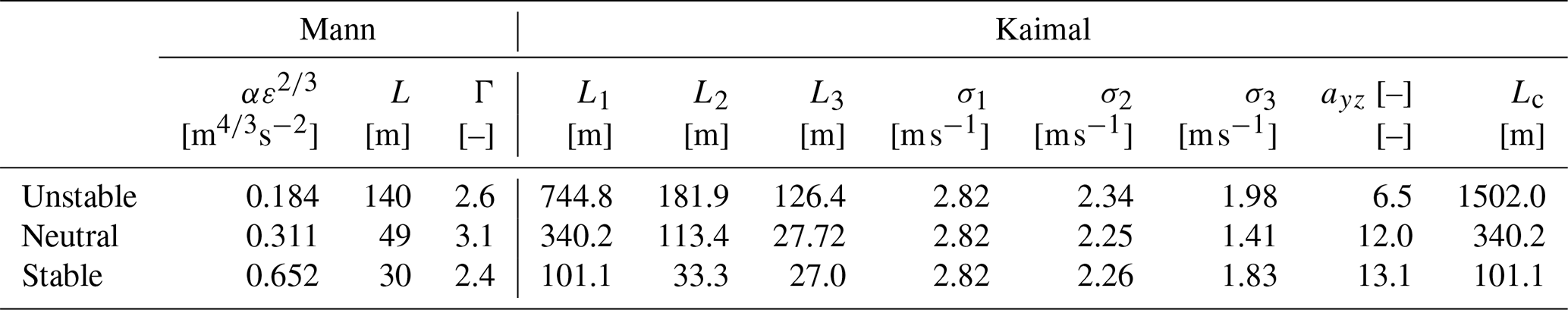
As for the Kaimal model, we chose the parameters listed by the IEC 61400-1:2019 (2019) for the neutral stability because these parameters were already found to give similar spectra and coherence compared to the Mann model with neutral stability parameters. Also, keeping these parameters allows readers to compare the results with those from existing literature, e.g., Schlipf (2015), Simley et al. (2018), and Dong et al. (2021). For unstable and stable stability classes, we fit the Kaimal spectra by the Mann-model-based spectra using the following optimization process:
Here, n is the index of the discrete frequency vector fn and wavenumber vector k1,n, N is the size of the discrete vector, and s.t. denotes “subject to”. Note that the Mann model spectra Fii(k1,n) are multiplied by 2 since they are the two-sided spectra, while the Kaimal spectra are single-sided. Similarly, we fit the yz plane exponential coherence for the Kaimal model by the Mann model using
where the fitting uses the co-coherence and ignores the quad-coherence. We fit the co-coherence instead of the magnitude-squared coherence, because the exponential coherence model (Eqs. 13 and 19) only includes the real co-coherence, whereas the coherence of the Mann model includes both co-coherence and quad-coherence. The medium separation m has been chosen for the optimization problem. For both optimization equations, the squared error in each discrete vector is divided by k1,n to ensure equivalent weighting of the optimization function at a different frequency or wavenumber ranges. The fitted spectra and yz plane coherence are shown by Fig. 2a and b, and the turbulence parameters are summarized in Table 1.
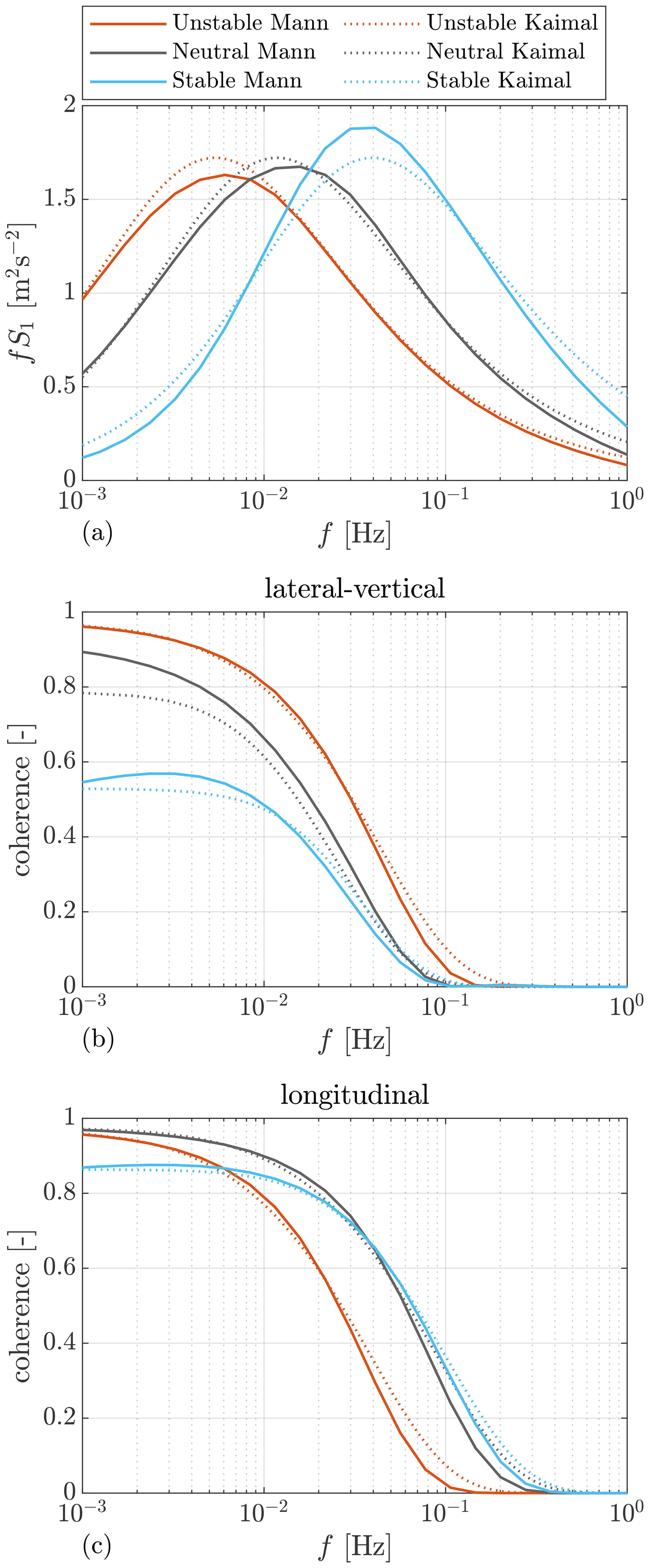
Figure 2(a) The auto-spectra of the longitudinal velocity component under different stability classes. (b) Lateral–vertical coherence of the longitudinal velocity component calculated using the Mann spectral tensor and fitted by the exponential coherence model. Note the co-coherence is shown for the Mann spectral tensor. (c) Longitudinal coherence of the longitudinal velocity component calculated using the space–time tensor and fitted by the exponential coherence model. The results are calculated with a mean wind speed of 16 m s−1.
Except for the spectra and yz plane coherence, Guo et al. (2022a) showed that the longitudinal coherence is related to the atmospheric stability based on measurement. In their study, a smaller intercept was found for a more stable class. Also, Simley and Pao (2015) studied the turbulence evolution under different stability classes using LES, and the smaller intercept was also observed in stable atmospheric (as shown in Fig. 2). In order to compare the longitudinal coherence under different atmospheric stability, we use three sets of , and 600 s to calculate the longitudinal coherence based on the space–time tensor Θ. The reason for choosing these values for γ is that they result in coherence close to observations in existing literature, as will be discussed later at the end of this section. Afterward, we fit the exponential coherence (Eq. 19) using the following optimization process:
Here we chose to fit the separation at Δx=100 m, which is the medium separation for a commercial lidar measuring in front of the turbine (Simley et al., 2018; Guo et al., 2022b). The fitted coherence is shown in Fig. 2c. The fitted exponential coherence parameters ax and bx are summarized in Table 2, and they show similar trend as the observation by Simley and Pao (2015) using LES. For an unstable atmosphere, ax is generally larger, and bx is in a very small order close to zero. In the neutral condition, ax lies in a medium value, and bx is also a small order close to zero. As for the stable case, ax is the smallest, meaning a weaker coherence decay, while bx is larger, resulting in a smaller intercept.
Table 2The fitted parameters for the exponential longitudinal coherence model.
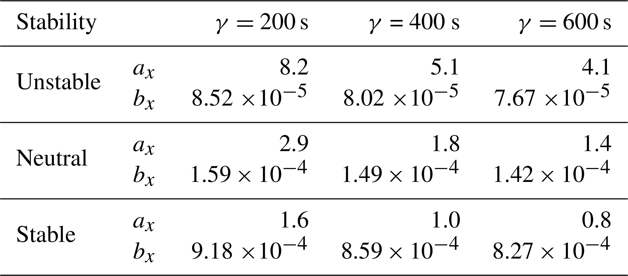
Based on the study by Guo et al. (2022a), γ was found to be 430 and 207 s for neutral and stable stability classes, respectively, while the value of γ in the unstable scenario has not been derived due to a lack of samples from measurement. Chen et al. (2021) performed a probability study of the coherence parameter ax based on lidar measurement, and it is found to appear between one and two with a higher probability. According to the analysis by Simley and Pao (2015), ax tends to be the largest in an unstable condition compared to that in a neutral or stable condition. Based on the previous observations by these authors, and since γ= 200 or 400 s gives unrealistically large values of ax in the unstable atmosphere that are less likely to happen, we decided to choose γ= 600 s for the unstable condition, which results in ax=4.1. And γ= 400 and γ= 200 are used for neutral and stable stability classes, respectively. In addition, it is worth mentioning that we do not consider the dependence of the turbulence evolution parameters on TI level. The selection of turbulence evolution parameters is based on relevant studies, and typical values are chosen. As studied by Simley and Pao (2015), the TI values can be different for the same atmospheric stability, and the evolution parameters show some dependence on the TI values. In the future, a joint probabilistic study on the turbulence spectral parameters, TI levels, and evolution parameters is necessary for defining more realistic simulation scenarios for LAC.
In this section, the definitions of REWS and the REWS estimated by lidar will first be discussed. Then the auto-spectra of these two signals and the cross-spectrum between them will be presented. In the end, we summarize the wind preview quality of the investigated four-beam lidar for the NREL 5.0 MW reference turbine under different atmospheric stability classes.
3.1 Rotor-effective wind speed
As discussed by Schlipf (2015), one way of defining the rotor-effective wind speed for control purpose is the mean longitudinal component u over the turbine rotor-swept area:
where D denotes the integration over the rotor area defined by rotor radius R.
For the Mann model, as derived by Held and Mann (2019), the auto-spectrum of the REWS uRR can be calculated using the spectral tensor by
with and J1 the Bessel function of the first kind. The detailed derivation of the auto-spectrum can be found in the works by Held and Mann (2019) and Mirzaei and Mann (2016).
As for the Kaimal model, the spectrum is derived by Schlipf et al. (2013a) and Schlipf (2015), i.e.,
where Δyzij is the separation distance between point i and j in the same yz plane, and nR is the total number of points in the rotor area. The detailed derivation of the auto-spectrum can be found in Schlipf (2015).
3.2 Lidar-estimated rotor-effective wind speed
Lidar utilizes the Doppler spectrum contributed by the aerosol backscatters within the probe volume to determine wind measurement. It is necessary to include the probe volume averaging effect. Mann et al. (2009) show that the lidar LOS measurements at a focus position can be approximated by
where is a unit vector aligned in the direction of a lidar beam that can be simply calculated after knowing the azimuth angle ϕ and elevation angle β (see Fig. 3 for the definition). r is the displacement along the lidar beam direction from the focused position x. φ(r) is the weighting function due to the lidar volume averaging. In this work, a typical pulsed lidar is considered whose weighting function is modeled by a Gaussian-shape function (Schlipf, 2015)
where the full width at half maximum WL is about 30 m.
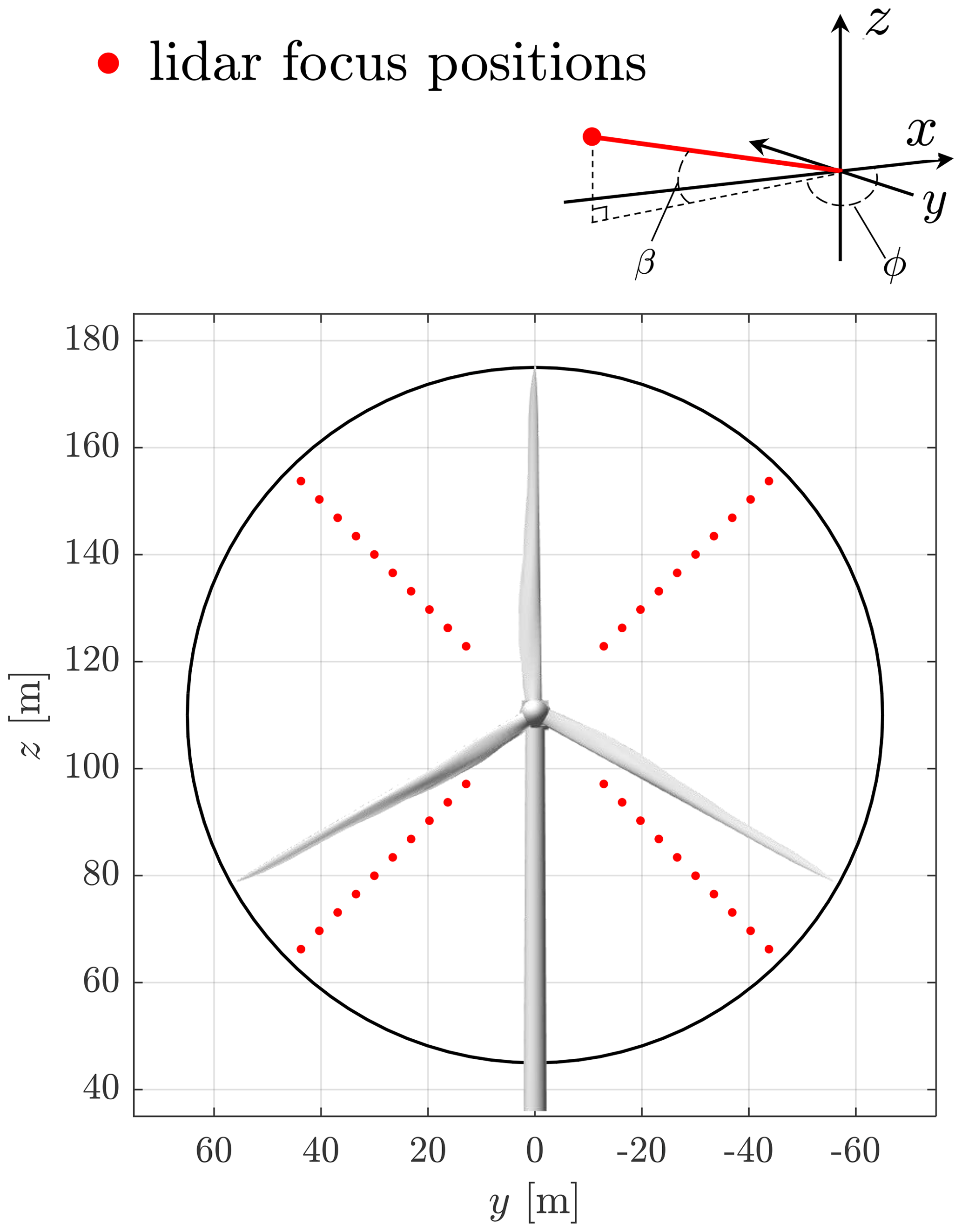
Figure 3The front view of the NREL 5.0 MW turbine and the optimized four-beam trajectory. A reference coordinate system for the lidar system is also shown, where the positive x direction is the mean wind flow direction.
Since lidar only provides the wind speed in the LOS direction, the u component is needed to be reconstructed from LOS speed. A simple algorithm is used to assume zero v and w components because they usually contribute much less than the u component to the LOS speed. In fact, this is true if lidar beam misalignment to the longitudinal direction is small. Based on this assumption, the lidar-estimated rotor-effective wind speed is often obtained by (see Schlipf, 2015)
where nL is the total number of lidar measurement positions, vlos,i(x) denotes the ith lidar measurement position, ϕi is the azimuth angle of the ith measured position, and βi is the elevation angle of the ith measured position.
Guo et al. (2022a) suggested calculating the auto-spectrum of the lidar-estimated REWS (uLL) from the Mann-model-based space–time tensor by
where xi and ni denote the focus position vector and the unit vector of the ith lidar measurement, respectively, nil is the lth element in the unit vector ni,
is the Fourier transform (non-unitary convention) of the weighting function of lidar, and is the time required for turbulence to propagate from position xi to xj. A more detailed derivation of Eq. (30) can be found in the works by Mirzaei and Mann (2016), Held and Mann (2019), and Guo et al. (2022a). In practical lidar data processing for wind turbine control, as discussed in Sect. 4.2, the lidar measurement data from different measurement gates are phase shifted to the nearest used measurement range gate using Taylor (1938)'s frozen hypothesis. This means that vlos,i(t) in Eq.( 29) should be shifted in time according to the mean wind speed and the longitudinal separation, i.e.,
where xnrg is the longitudinal position of the used measurement range gate nearest to the rotor plane. As a consequence, the phase shifts contributed by longitudinal separations (xi−xj) in Eq. (30) are always zero.
For the Kaimal model, the auto-spectrum can be derived based on the Fourier transform:
where ℱ{ } denotes the Fourier transform. The Fourier transform of the ith LOS speed vlos,i is quite lengthy and thus is not extended here. The detailed expression can be found in the work by Chen et al. (2022).
3.3 Cross-spectrum between rotor and lidar
When turbulence evolution is considered with the Mann model, Guo et al. (2022a) show that the cross-spectrum between REWS uRR and the lidar-estimated one uLL can be calculated using the space–time tensor by
where Δti is the time required for the turbulence field to move from the ith lidar measurement position to the rotor plane, which can be approximated by . Here, Δxi is the longitudinal separation between the rotor plane and the ith lidar measurement position and , with xR being the rotor plane position on the x axis. For LAC, the lidar measurement data from different range gates are phase shifted to the rotor plane using Taylor (1938) frozen hypothesis; therefore, this assumption is also made when deriving Eq. (34).
Similarly, following Schlipf (2015), the cross-spectrum for the Kaimal model is
with ui the ith longitudinal wind component in the rotor swept area. See Chen et al. (2022) for detailed derivation of the Fourier transform of vlos,j, where the main algorithm is to loop over the Fourier transform of all velocity components included in ui and vlos,j.
3.4 Lidar wind preview and filter design: case analysis
To evaluate the preview quality of lidar measurement, one can calculate the lidar–rotor coherence by
Then, a measurement coherence bandwidth (the wavenumber at which the coherence drops to 0.5, noted as k0.5) can be found. Note that , where f0.5 is the frequency at which the coherence drops to 0.5. k0.5 and is usually used as the optimization criteria for the LAC-oriented lidar measurement trajectory (Schlipf et al., 2018a).
In this work, we chose the medium-size NREL 5.0 MW reference wind turbine with a rotor diameter of 126 m (Jonkman et al., 2009) and a typical four-beam pulsed lidar trajectory (e.g., WindCube Nacelle and Molas NL). The lidar trajectory is firstly optimized following the method proposed by Schlipf et al. (2018a) using the space–time tensor-based lidar–rotor coherence γRL. The turbulence parameters corresponding to the neutral stability in Table 1 are considered in the optimization process. The optimized trajectory parameters of the used lidar are given in Table 3. A front view of the lidar and turbine geometry is shown in Fig. 3.
Table 3Parameters of the optimal four-beam pulsed lidar system. Optimized according to the measurement coherence bandwidth using the space–time tensor model. The definitions of the angles are shown in Fig. 3.

With the optimized lidar trajectory, we show the coherence γRL under different stability classes in Fig. 4a. It can be seen that the coherence using the Mann-model-based space–time tensor is generally better than that using the Kaimal model. For both models, the coherence in neutral and stable stability classes is higher than that in the unstable stability, which can be caused by stronger turbulence evolution in the unstable situation. The coherence in the unstable case is especially lower using the Kaimal model, which can be caused by the direct product method. Based on the investigation by Simley (2015) using LES, combining coherence using the direct product can underestimate the overall coherence.
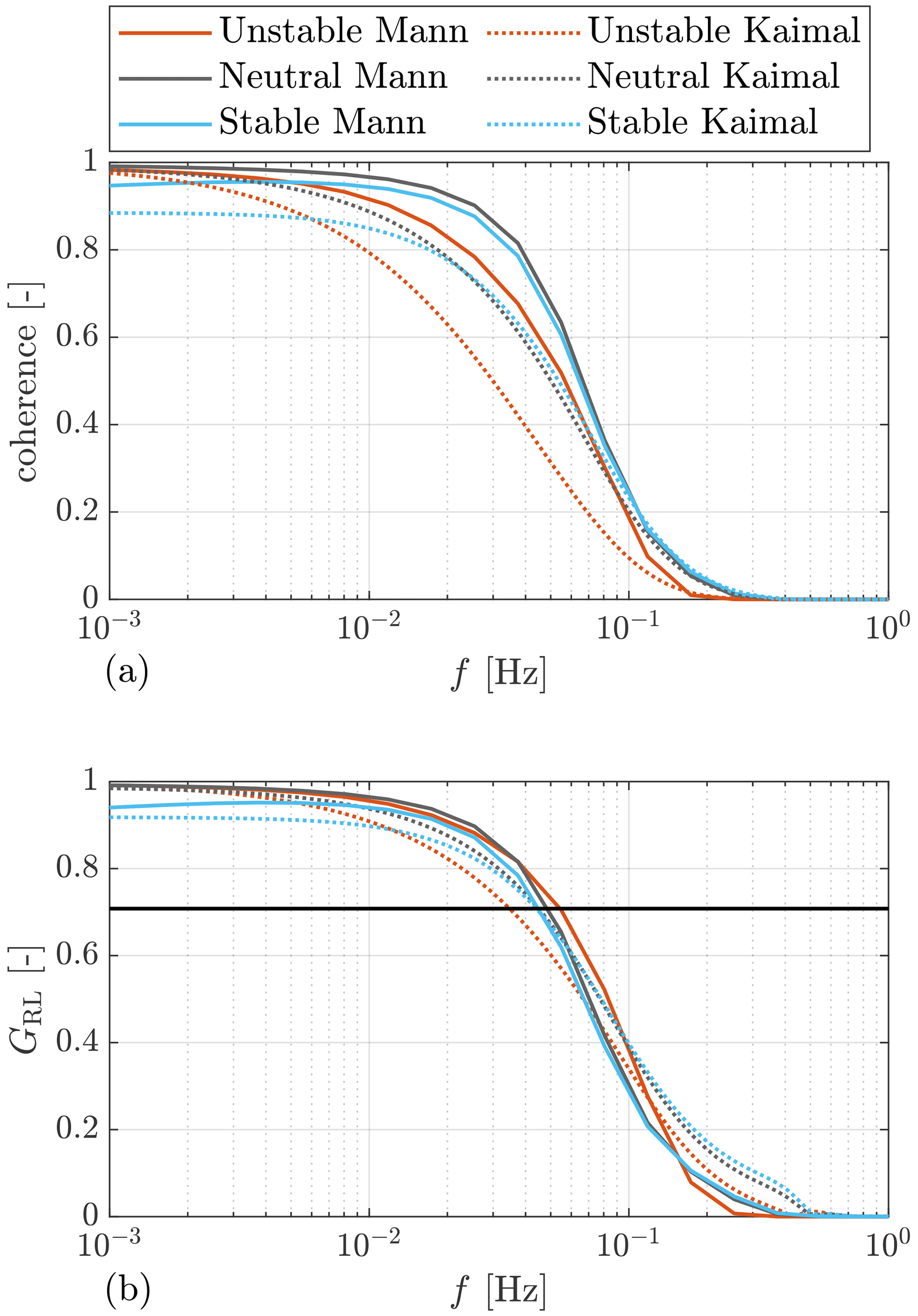
Figure 4(a) Coherence between lidar-estimated REWS and the turbine based REWS. (b) The optimal transfer function gain. The black dot line corresponds to the −3 dB magnitude. The results are calculated with a mean wind speed of 16 m s−1.
Except for the coherence, another indicator of how well the lidar predicts the REWS can be the following transfer function (Schlipf, 2015; Simley and Pao, 2013):
If a filter is designed to have a gain of GRL(f), it turns out to be an optimal Wiener filter (Simley and Pao, 2013; Wiener, 1964), which produces an estimate of a desired or target signal (here the uRL). The Wiener filter minimizes the mean square error between the target signal and the estimate of the signal. When used for LAC, if the system is modeled as a system with two inputs, REWS and lidar-estimated REWS, and one output, rotor speed, the Wiener filter leads to minimal rotor speed variance as formulated by Simley and Pao (2013). At a certain frequency, the larger gain means that less information needs to be filtered out before the signal is used. So, it indicates how much information measured by the lidar is usable for feedforward control.
The transfer functions under the three investigated stability classes are shown in Fig. 4b. The transfer function gains are similar in the three stability classes for the space–time tensor-derived results. As for the results by the Kaimal model, the transfer function gain is lower in unstable stability but similar in neutral and stable stability classes.
By the turbulence spectral model, which represents the mean spectral properties, we can obtain the expected Wiener transfer function gain. However, in real operation, the Wiener filter design is more complicated and requires a higher-order filter. In contrast, a linear filter that has similar damping as the Wiener filter can also provide a similar filtering effect as the Wiener filter. The linear filter is usually designed to have a cutoff frequency at −3 dB of the Wiener filter (see Schlipf, 2015, and Simley et al., 2018). The cutoff frequencies as a function of mean wind speed are calculated by fitting the GRL and are shown in Fig. 5. Note that the TI value is also adjusted using the mean wind speed according to the IEC 61400-1:2019 (2019) standard. Firstly, both turbulence models indicate that the cutoff frequencies depend on the mean wind speed linearly. Therefore, the cutoff frequency of the filter can be scheduled based on this linearity. Generally, the cutoff frequencies by the Mann-model-based space–time tensor are generally larger than those by the Kaimal model. For the same turbulence model, the resulting cutoff frequency does not change significantly by the analyzed turbulence stability conditions. The largest difference appears at the highest mean wind speed 24 m s−1, where the difference of cutoff frequency between unstable and stable conditions is about 0.02 Hz. As for lower mean wind speed (≤ 18 m s−1), it can be seen that the turbulence parameters of different atmospheric stability classes do not influence the cutoff frequency very much, and the difference is smaller than 0.01 Hz. This also indicates that, for mean wind speed ≤ 18 m s−1, the filter design is not very sensitive to the change in turbulence parameters related to atmospheric stability, and a constant filter design is robust. In the rest of this work, we will use the constant cutoff frequency derived from neutral stability for both the Mann-model-based and the Kaimal-model-based simulations. For example, 0.0490 and 0.0449 Hz will be used, respectively, for the Mann model and the Kaimal-model-based simulations with a mean wind speed of 16 m s−1. However, for a mean wind speed above 20 m s−1, using the cutoff frequency derived from neutral stability is relatively biased from the cutoff frequency derived for unstable conditions. The impact of this non-ideal filtering should be analyzed further in future works.
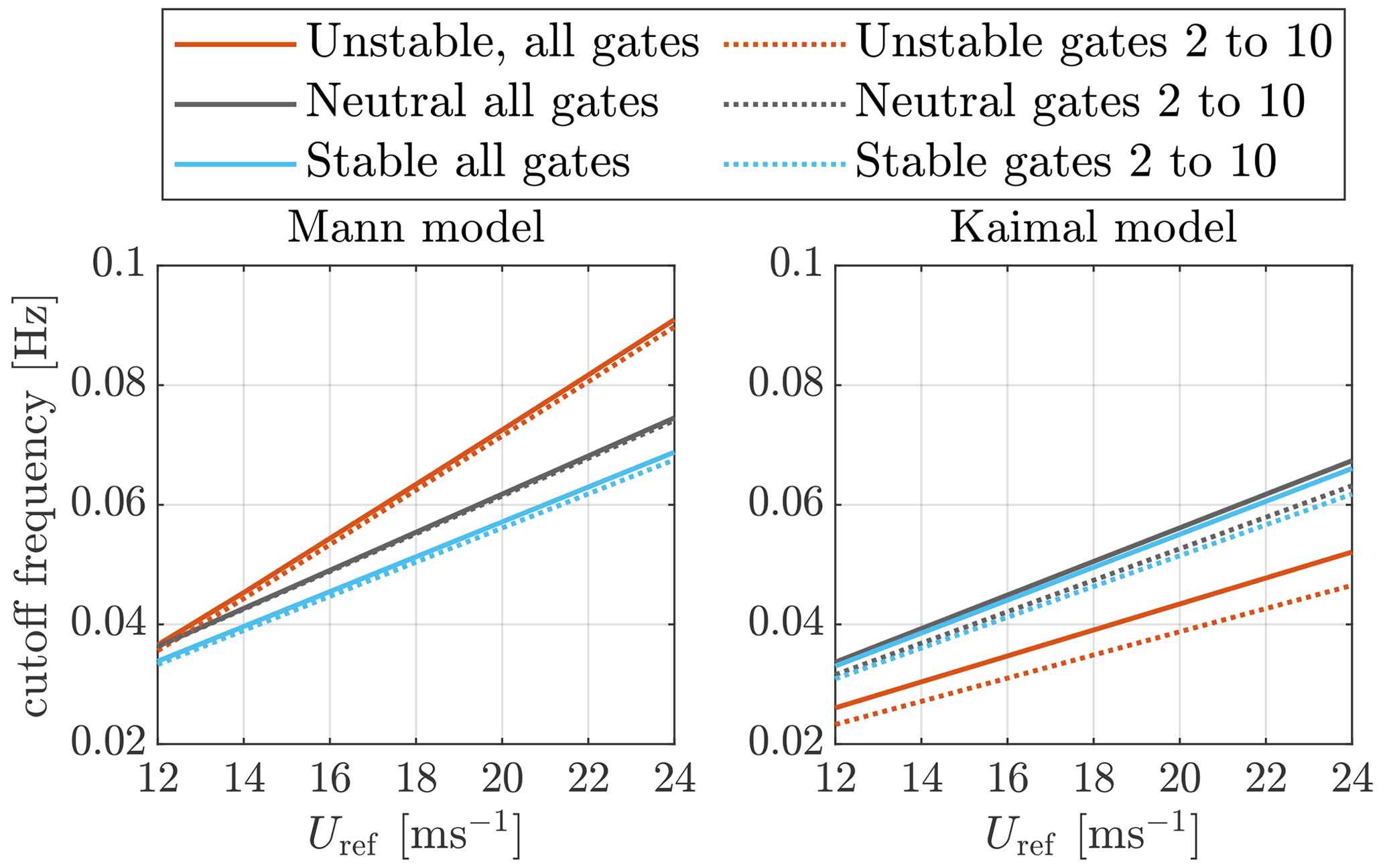
Figure 5The dependency of cutoff frequencies in hertz on the mean wind speed. The cutoff frequency corresponds to −3 dB at the GRL magnitude. In “all gates” the lidar measurement gates from 1 to 10 are considered. In “gates 2 to 10” the lidar measurement gates from 2 to 10 are considered.
Apart from the case that all measurement gates (see the caption of Fig. 5) are considered, another case, where nine lidar measurement gates are considered, is also shown in Fig. 5. It can be clearly seen that the cutoff frequencies are only slightly reduced when the first measurement gate is ignored. The reason for considering nine measurement gates is that the leading time of the lidar-estimated REWS needs to be larger than the time delays caused by filtering, by time-averaging over the full lidar scan, and by the pitch actuator. The leading time of the first measurement gate can be insufficient for very high wind speed, and it must be ignored. A more detailed discussion about the leading time and time delay will be discussed in Sect. 4.4.
In this section, we introduce the lidar-assisted turbine controller theory and its integration into OpenFAST aeroelastic simulation.
4.1 Data exchange framework
To configure LAC in the OpenFAST aeroelastic simulation, we chose to use the Bladed-style interface (DNV-GL, 2016). The interface is responsible for exchanging variables between the OpenFAST executable and the external controllers compiled as a dynamic link library (DLL). To make each controller as modular as possible, we programmed an open-source main DLL (written in FORTRAN), namely the “wrapper DLL”. The main function of the wrapper DLL is to call the sub-DLLs by a specified sequence. Note that all the sub-DLLs work based on the same variable exchange pattern specified by the Bladed-style interface. This means each sub-DLL can also be called by OpenFAST independently and directly. Or, several sub-DLLs can be called by the wrapper DLL together. An overview of the LAC and OpenFAST interface is shown in Fig. 6. Three sub-DLLs will be called by the wrapper DLL following the sequence from up to below in the figure. The source code of a baseline version of these DLLs has been made openly available (see “Code availability”).
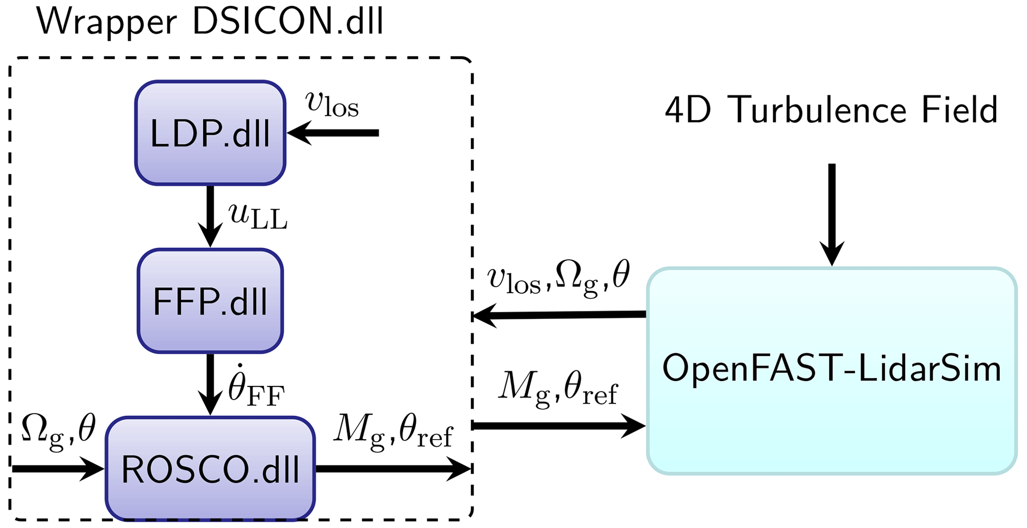
Figure 6The overall OpenFAST and LAC interface. LDP: lidar data processing. FFP: feedforward pitch. ROSCO: the reference FB controller.
4.2 Lidar data processing
As mentioned before, the lidar measurement data need to be processed before they can be used for control. The first sub-DLL is the lidar data processing (LDP) which calculates the lidar-estimated REWS from the lidar LOS speed.
In reality, the lidar usually does not measure all beam directions simultaneously. Instead, it sequentially measures from one direction to the next direction. This sequential measurement property is later simulated using the lidar module in the aeroelastic simulation (see Sect. 5.1.1). Therefore, a time-averaging window needs to be applied to estimate the REWS from a full LOS scan. For the four-beam lidar used in this work, the averaging window is chosen to be 1 s, which is the time required to finish a full scan by four beams. To apply the averaging window, the LDP module also needs to record the leading time of the successful measurement. The leading time can be approximated by . When estimating the REWS, only the LOS measurements whose leading times are within the time-averaging window will be chosen, and then Eq. (32) is applied to estimate the REWS. Besides, the blade blockage effect is considered in the simulation, and this phenomenon is included in the updated OpenFAST lidar module (Guo et al., 2022b). Due to the blade blockage, the LOS measurements for a certain lidar beam are not always available. Therefore, the LDP module estimates the REWS only using all the available LOS measurements.
4.3 Feedback-only controller
A typical variable-speed wind turbine is controlled by a blade pitch and generator torque controller. A baseline collective feedback blade pitch control is achieved by a proportional-integral (PI) controller (Jonkman et al., 2009):
where θFB is the feedback pitch reference value, Ωg,ref is the generator speed control reference, Ωgf is the measured and low-pass-filtered generator speed, kp is the proportional gain, TI is the integrator time constant, and s is the complex frequency. The pitch controller is only active in the above-rated wind speed, and kp and TI are scheduled to have a constant closed-loop behavior through gain scheduling (Abbas et al., 2022). For the NREL 5.0 MW wind turbine, the desired damping and angular frequency are tuned to be 0.7 and 0.5 rad s−1, respectively.
For better code accessibility, the recently developed open-source reference controller, ROSCO (v2.6.0) by Abbas et al. (2022), is used as the reference FB-only controller. ROSCO uses a PI controller for the pitch control in the above-rated wind speed operation. In terms of generator torque control in the above-rated operation, we have chosen the option of constant power mode in our simulations, with which the generator torque is set according to the filtered generator speed to keep the electrical power close to its rated value. The generator torque (Mg) is set according to the low-pass-filtered generator speed, the rated electrical power (Prated), and the generator efficiency (η) by . See the work by Abbas et al. (2022) for a more detailed description of the reference controller. We have modified the ROSCO source code to allow it to accept the feedforward pitch rate signal. The feedforward pitch rate (see next section) is added before the integrator of the PI controller.
4.4 Combined feedforward and feedback controller
The collective feedforward pitch control proposed by Schlipf (2015) is used in this work where the feedforward pitch reference value is obtained by
with uLLf the filtered REWS estimated by lidar and θss the steady-state pitch angle as a function of the steady-state wind speed uss. The steady-state pitch curve can usually be obtained by running aeroelastic simulations using uniform and constant wind speed. Figure 7 shows the general control diagram with the lidar-assisted pitch feedforward signal θFF. In practice, the pitch time derivative of the pitch feedforward signal is fed into the integral block of the feedback PI controller. This gives the overall collective pitch control reference as
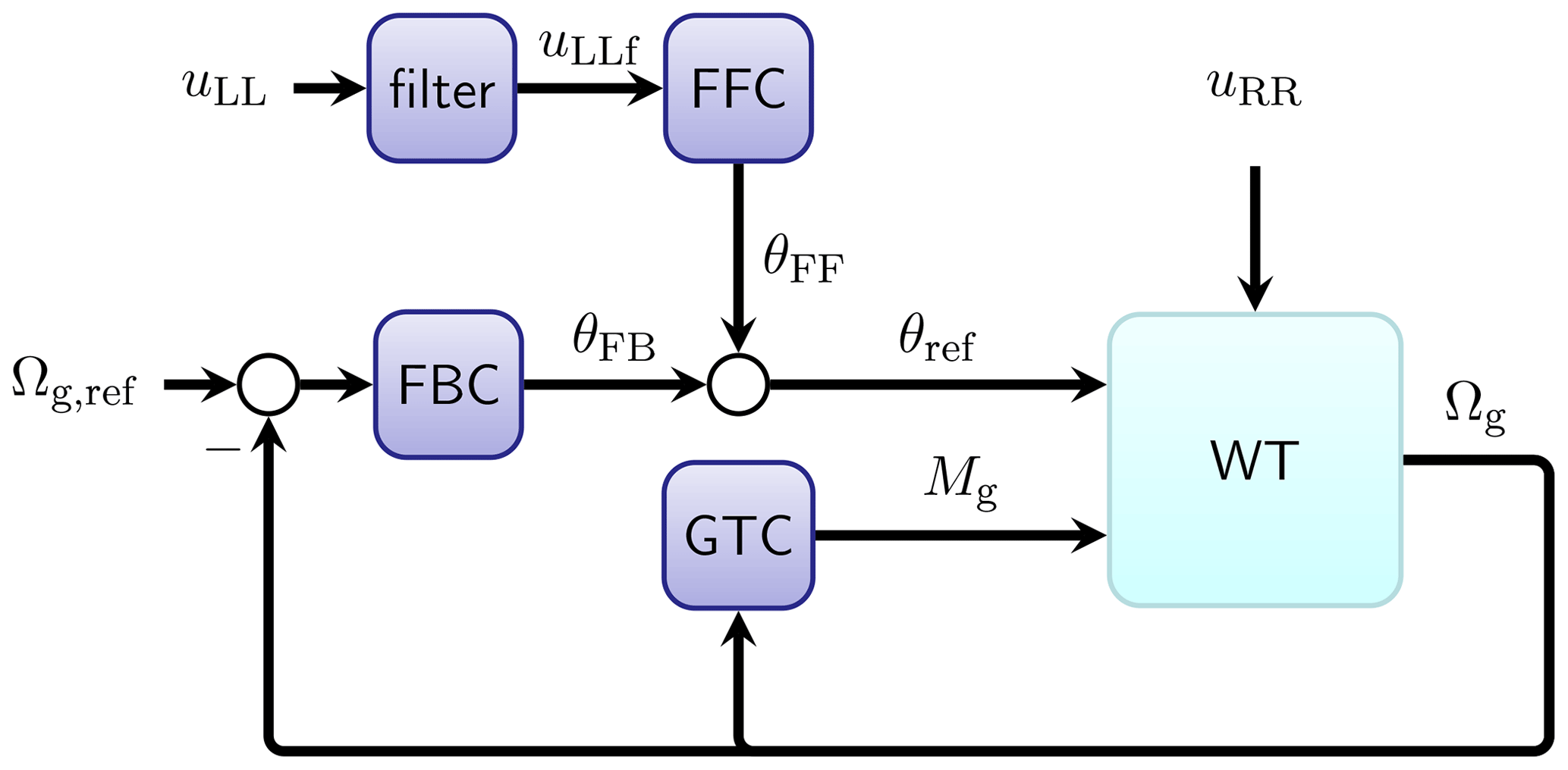
Figure 7The overall control diagram. FFC: feedforward pitch controller; FBC: collective feedback pitch controller; GTC: generator torque controller. Note that the real-time pitch angle (θ) signal is also used in the FBC and GTC for controller scheduling.
A feedforward pitch (FFP) sub-DLL is programmed to be responsible for filtering the lidar-estimated REWS and provide feedforward pitch rate at correct time. A first-order low-pass filter with the following transfer function:
where fc is the cutoff frequency, as discussed in Sect. 3.4, that is applied to filter the uLL signal. Based on the filter cutoff frequency, the time delay introduced by the low-pass filtering of lidar-estimated REWS (Tfilter) can be estimated (see Schlipf, 2015, for detailed calculation). The pitch feedforward signal is then sent to ROSCO after accounting for the pitch actuator delay (Tpitch), the filter delay, and the half of the time-averaging window (Twindow). That is, the signal recorded in the timing buffer that has a time close to the buffer time is activated. The buffer time is defined as
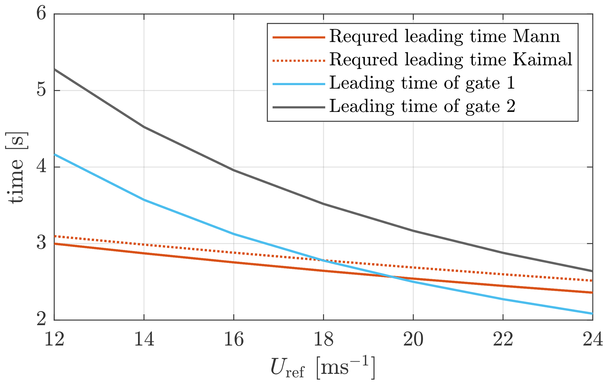
Here, Twindow= 1 s is the time-averaging window equivalent to one full scan time of the lidar. It is multiplied by in Eq. (42), because of the phase delay property of the time-averaging filter (Lee et al., 2018). The actuator delay is chosen to be Tpitch=0.22 s based on the phase delay of the pitch actuator. The actuator is modeled as a second-order system with a natural frequency of 1 Hz and a damping ratio of 0.7 (Dunne et al., 2012). Figure 8 shows the leading time (Tlead) by the first two measurement gates and the required leading time (). For the mean wind speed range where the leading time of gate 1 is lower than the required leading time, we only use the lidar measurement gates from 2 to 10 for estimating the REWS. The leading time of gate 2 is sufficient to provide enough leading time for all the considered mean wind speeds.
Another point for the feedforward pitch command is that it is only activated when the REWS is above 14 m s−1. The reason for setting this threshold value is that the pitch curve has much higher gradients with respect to wind speed in the range between 12 and 14 m s−1 (Schlipf, 2015), where the turbine thrust is the highest. If the feedforward pitch is activated only depending on the lidar-estimated REWS, a short interval of wind rise or drop in this range can cause a relatively large pitch rate and change in thrust force. Then the benefits of LAC are offset by the additional load caused by these pitch actions.
In this section, we use the open-source aeroelastic simulation tool OpenFAST to further evaluate the benefits of LAC. The simulation results will be presented and discussed.
5.1 Simulation environment
5.1.1 Lidar simulation
Previously, OpenFAST (v3.0) was modified to integrate a lidar simulation module (Guo et al., 2022b). The lidar simulation module includes several main characteristics of nacelle lidar measurement: (a) lidar probe volume, (b) turbulence evolution (lidar measures at the upstream wind field), (c) the LOS wind speed affected by the nacelle motion, (d) lidar beam blockage by turbine blade, and (e) adjustable measurement availability. Based on the study by Guo et al. (2022b) the blade blockage does not have an impact on the lidar measurement coherence for above-rated wind speed operation, but special treatment needs to be made to process the invalid measurement caused by the blade blockage effect. In this work, a similar algorithm discussed by Guo et al. (2022b) is used to process the invalid measurement data. Also, the data unavailability caused by low back scatters is not considered. Therefore, the unavailable data are only caused by the blade blockage.
5.1.2 Stochastic turbulence generation
To include the turbulence evolution for the aeroelastic simulation, four-dimensional stochastic turbulence fields are required. We use the newly developed 4D Mann Turbulence Generator (Guo et al., 2022a) and evoTurb (Chen et al., 2022) to generate the Mann-model- and Kaimal-model-based 4D turbulence fields, respectively. The turbulence parameters representative for three atmospheric stability classes are used (see Table 1 in Sect. 2).
For the turbulence field generated by the 4D Mann turbulence generator, since it only contains the fluctuation part of the turbulence, we add the mean field (only for u component) considering a power law shear profile with a shear exponent of 0.2. Each 4D turbulence field has a size of grid points, corresponding to the time and the x, y, and z directions. The lengths in the y and z directions are both 310 m, which is much larger than the rotor size. The reason for choosing this size is to avoid the periodicity of the turbulence field in y and z directions (Mann, 1998).
For the Kaimal-model-based 4D wind fields, evoTurb is used, which calls on Turbsim (Jonkman, 2009) to generate statistically independent 3D turbulence field and then composite 4D turbulence with the exponential longitudinal coherence discussed in Sect. 2. Only the coherence of the u component is considered, and the rest of the velocity components are not correlated. Similarly, the mean field (only for u component) is considered to be a power law shear profile with a shear exponent of 0.2. Each turbulence field has a size of grid points, corresponding to the time and the x, y, and z directions. The lengths in the y and z directions are both 150 m, which are enough to simulate the aerodynamic of the 126 m rotor of the NREL 5.0 MW turbine. Note that the Kaimal-model-based wind fields do not have the issue of periodicity so that the field size is not as large as that of the Mann-model-based fields.
For both types of 4D turbulence fields, the time step is chosen to be 0.5 s, and the hub height mean wind speed from 12 to 24 m s−1 with a step of 2 m s−1 is considered. The turbulence parameters are chosen based on Table 1. However, , σ1, σ2, and σ3 are adjusted according to the mean wind to reach the TI corresponding to class 1A, as specified in IEC 61400-1:2019 (2019). The positions in the x direction both contain the rotor plane position and the lidar range gate positions (see Table 3). Taylor (1938)'s frozen theory is applied within the probe volume, which has been shown not to influence the lidar measurement spectral properties by Chen et al. (2022). For example, the lidar measurement gate at x=50 m is calculated using the yz plane wind field at x=50 m, which is then shifted with Taylor's frozen theory to count for the lidar probe volume averaging. The time length of each field is 2048 s.
5.1.3 Simulation setup
For each stability class, we generate 4D turbulence fields with 12 different random seed numbers. For each turbulent wind field, the OpenFAST simulation is executed with the following configurations: (a) FB control using ROSCO only and (b) feedforward+feedback (FFFB) control using lidar measurements. All the degrees of freedom for a fixed-bottom turbine except for the yawing are activated. Each simulation is executed for 31 min. For each simulation, we remove the initial 60 s time series, which contains the initialization.
5.2 Results and discussion
5.2.1 Time series
In Fig. 9, we take the one simulation (with a mean wind speed of 16 m s−1) using the 4D Mann turbulence generator with the neutral stability condition as an example to show the time series.
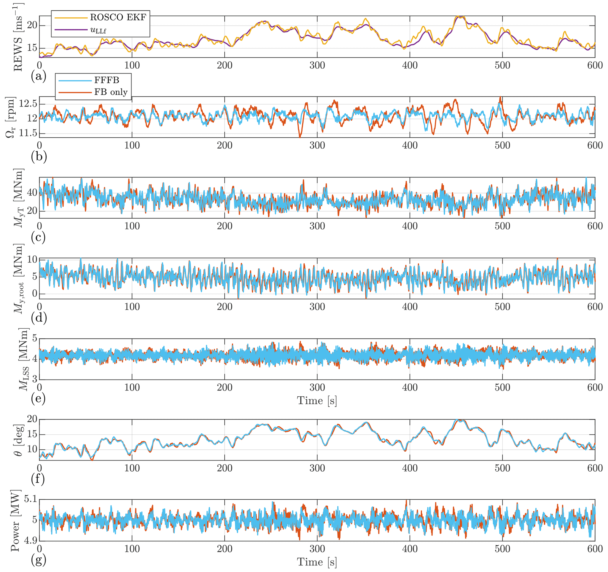
Figure 9The time series collected from OpenFAST simulation. The case with the Mann model and neutral stability parameters is shown. Note the same 3D wind field is applied to the rotor when performing simulations with the FFFB control and the FB-only control. Simulated with a mean wind speed of 16 m s−1. EKF: extended Kalman filter.
Panel (a) compares the REWS estimated by the lidar data processing algorithm and that estimated by the extended Kalman filter (EKF) (Julier and Uhlmann, 2004) implemented in ROSCO. The lidar-estimated REWS is shifted according to the time buffer by the FFP module so that it does not show any time lag in the plot. The lidar-estimated REWS shows good agreement with that estimated by the Kalman filter. It can be seen that some additional fluctuations with higher frequency appear in the time series of ROSCO-based REWS. This can be caused by the fact that ROSCO only uses a model with 1 degree of freedom containing the rotor rotational motion and all the other structural motions affecting the rotor speed can be “mistakenly” estimated as wind speed.
Panel (b) shows that the rotor speed obviously fluctuates less using FFFB control compared to that using FB control only. Also, the peak values with FFFB control are smaller.
The tower fore–aft bending moment MyT is compared in panel (c), where it is generally less fluctuating with the help of LAC. Further, the blade root out-of-plane bending moment (My,root) is shown by panel (d), in which FFFB slightly reduces the fluctuation compared to FB-only control. The low-speed shaft torques (MLSS) are compared in panel (e). Again it is clear that the fluctuation with FFFB control is a bit lower than that with FB-only control.
In panel (f), we show the pitch action between the two control strategies. The pitch angles in the FFFB control generally lead that by the FB-only control in time, as expected. The pitch angle trajectories are overall similar between the FFFB and FB-only controls.
Lastly, the generator power is shown in panel (g). Here, we can see that the generator power fluctuates even though the constant power torque control mode is activated. The reason is that ROSCO uses low-pass-filtered generator speed to calculate the generator torque command by , as mentioned previously in Sect. 4.3. If we do not consider the fact that the turbine might have a short interval to reach below-rated operation during a wind speed drop, the formula above ensures that the electrical power is constant if the electrical power is calculated using the filtered generator speed. However, the actual electrical power is determined by the non-filtered generator speed, and the difference between the filtered and non-filtered generator speeds determines the power fluctuation. Because the difference is mainly the generator speed fluctuations of high frequencies, we can see that the electrical power contains fluctuations of high frequencies. By comparing FFFB and FB-only controls, it can be seen that reduced low-frequency rotor speed fluctuations are observed in FFFB control. Because the low-frequency power fluctuation is highly coupled with the rotor speed fluctuation (see panel b), less fluctuating power can be expected from the less low-frequency rotor speed fluctuation in FFFB control.
5.2.2 Spectral analysis
We estimate the spectra from the collected time series using the Welch (1967) method. The spectra are averaged by different samples. Each sample is the aeroelastic simulation result produced by a turbulence field generated by a specific random seed number.
Before comparing the OpenFAST outputs spectra, the spectra of the REWS by the input turbulent wind fields are first compared in Fig. 10. Here, the simulated REWS is calculated by averaging the u components within the rotor-swept area from the discrete turbulent wind field. We show that the simulated spectra follow the theoretical ones well, which validates the turbulence simulation. In Sect. 2, the single-point u component spectrum by the two models is fitted. Also, the yz plane coherence is fitted using a single separation. Here, it can be seen that the REWS spectra by the two models show a similar trend in different atmospheric stability classes. In the unstable case, the REWS spectrum does not reduce a lot compared to a single-point u spectrum, and the spectrum peak appears at a lower frequency. This is because the turbulence field has more large-scale coherent structures in the unstable atmosphere, as depicted in Fig. 1. In the stable case, everything is opposite to the unstable case where the REWS spectrum is much lower compared to the single-point u spectrum because of the low-level coherence and the spatial filtering effect of the rotor. In addition, the neutral stability shows a medium spatial filtering effect, and the spectrum peak is between that of unstable and stable conditions. For each stability class, it can be seen that the Kaimal-derived REWS generally has a higher spectrum compared to that derived by the Mann model. This can be caused by the fact that the yz plane coherence by the Mann model is more complicated than the exponential coherence model used in the Kaimal model. Fitting the coherence using one separation is insufficient to represent all possible separations. By comparing the spectra by mean wind speeds of 16 and 18 m s−1, we observe that the spectral peaks are shifted to a higher-frequency side in all stability classes.
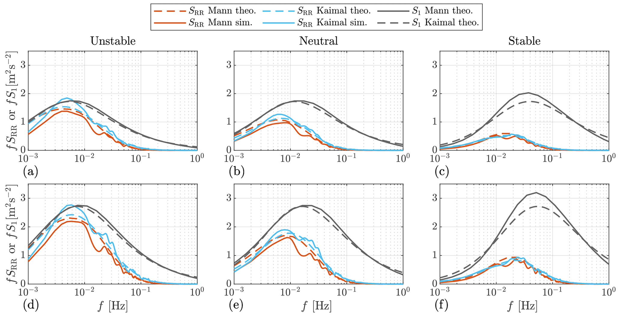
Figure 10The auto-spectra of REWS. “theo.”: theoretical spectra by the models discussed in Sect. 3, i.e., Eqs. (25) and (26). “sim.”: the spectra estimated from the time series of the turbulent wind fields in OpenFAST simulations, using the Welch (1967) method. S1: the auto-spectra of a single-point u component. Panels (a)–(c) have a mean wind speed of 16 m s−1. Panels (d)–(f) have a mean wind speed of 18 m s−1.
In Figs. 11 and 12, the auto-spectra of some of the most interesting output variables by FB-only control and FFFB control are compared. Figure 11 shows the results using the Mann model, and Fig. 12 shows the results using the Kaimal model.
Panels (a), (b), and (c) compare the rotor speed spectra between FFFB and FB controls under three stability classes. The FFFB control generally reduces the rotor speed spectrum in the frequency range from 0.01 to 0.1 Hz. It can also be seen that the spectra using the Mann model and the Kaimal model show some differences, which can be summarized as higher spectra of the rotor motion by the Kaimal model than that by the Mann model. However, the spectra estimated from simulated time series using the two models generally have similar shapes.
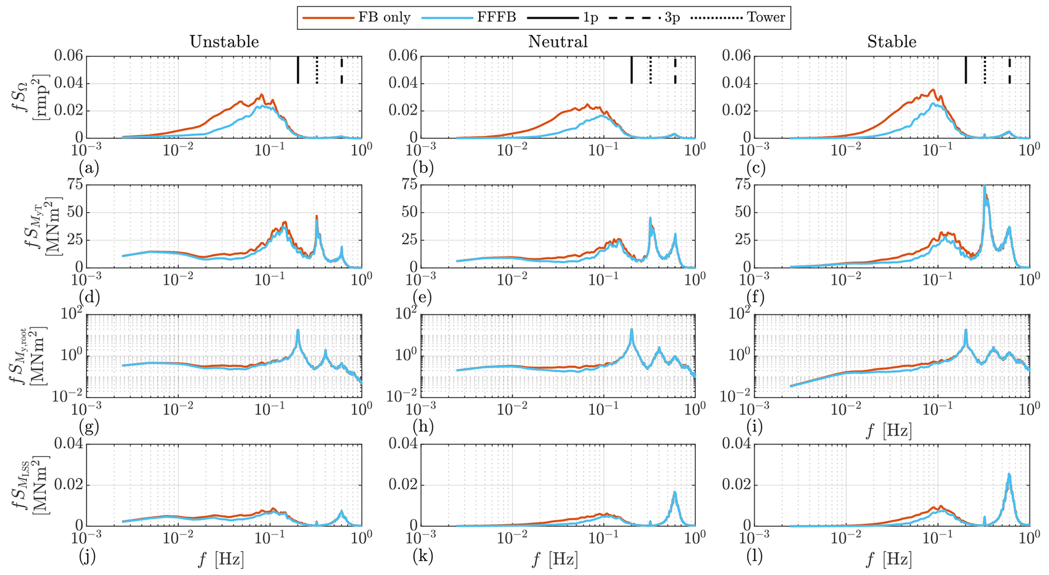
Figure 11The auto-spectra estimated from OpenFAST output time series. The simulation results are obtained using the Mann model. The mean wind speed is 16 m s−1. Note that the y axis of the blade root bending moment is set to logarithmic for better readability.
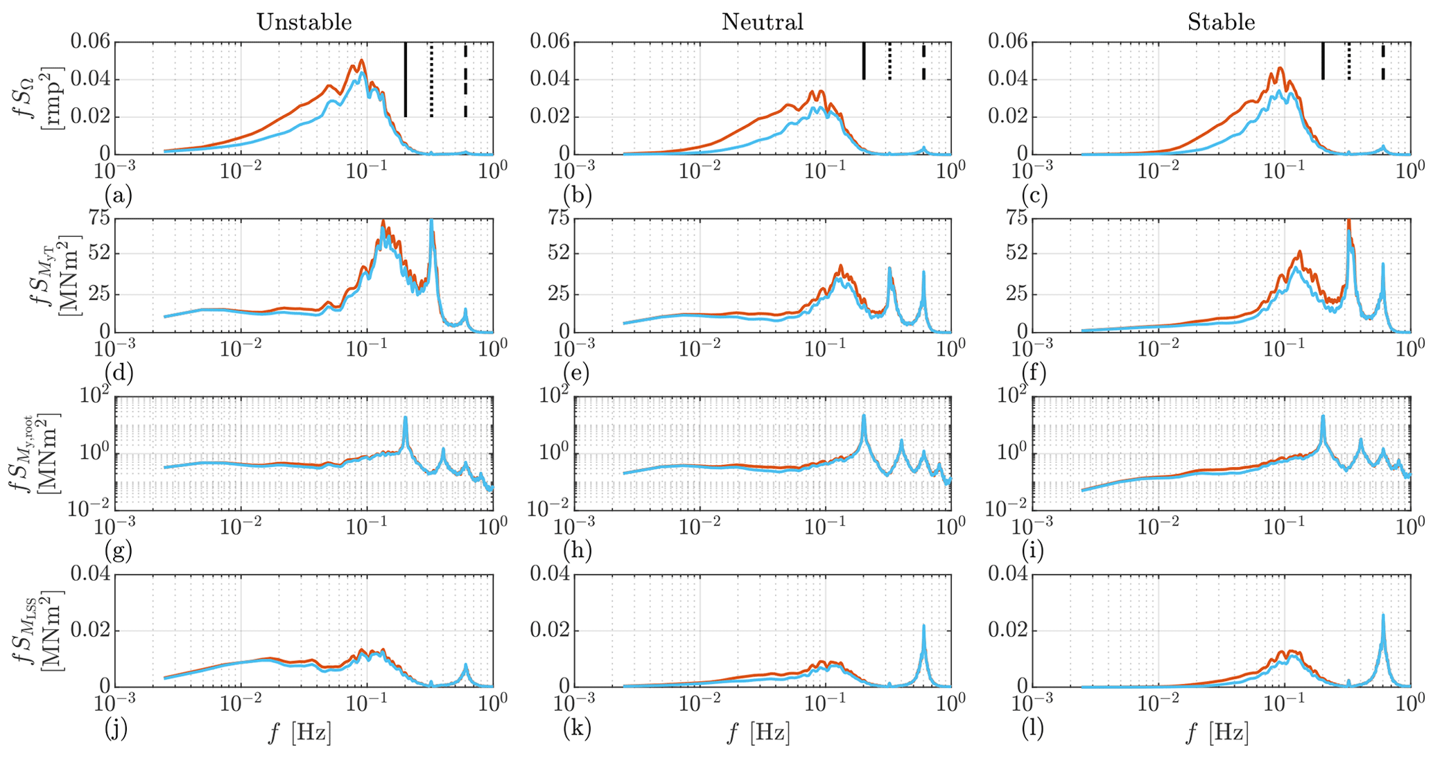
Figure 12The auto-spectra estimated from OpenFAST output time series. The simulation results are obtained using the Kaimal model. The mean wind speed is 16 m s−1. Note that the y axis of the blade root bending moment is set to logarithmic for better readability.
The comparison of the tower fore–aft bending moment is shown in panels (d), (e), and (f). In neutral and stable cases, the main benefits bought by FFFB control are the reductions in the frequency range from 0.01–0.2 Hz, which is as expected since the lidar–rotor transfer function (Eq. 37) becomes zero close to 0.2 Hz. Below 0.01 Hz, there are not many differences between FB-only and FFFB controls, because the tower fore–aft mode is naturally damped well in this frequency range.
Panels (g), (h), and (i) show the blade root out-of-plane moment of blade one. There are slight reductions in the blade root out-of-plane moment in the frequency range from 0.02 to 0.1 Hz contributed by LAC. It can also be seen that the spectrum is mainly composited by the excitation at the 1 p (once per rotation) frequency.
The comparison of low-speed shaft torque is shown by the panels (j), (k), and (l). Using FFFB control brings some benefits in the frequency range from 0.01 to 0.1 Hz, which is similar to the reduction range of the rotor speed.
Overall, the relative reductions in the spectra bought by adding FF control mainly lie in the frequency range where the lidar–rotor transfer function is above zero. For very low-frequency ranges, the turbine motions are naturally damped; thus, no obvious benefits are brought by adding the pitch feedforward signal. Based on the spectral analysis, we found reductions significantly in rotor speed, some in tower fore–aft moment, and slightly in low-speed shaft torque. Also, the reductions are observed by both turbulence models in three different atmospheric stability classes.
5.2.3 Simulation statistic
To further evaluate the benefits of LAC, we calculate the DEL using the rainflow counting method (Matsuishi and Endo, 1968) with 2 × 10⁶ as a reference number of cycles and a lifetime of 20 years. The Wöhler exponent of 4 is used for the tower fore–aft bending moment and the low-speed shaft torque, and the Wöhler exponent of 10 is used for the blade root out-of-plane bending moment. The averaged DEL is calculated from the results by different random seed numbers. The overall statistics are compared and shown in Figs. 13 and 14. For rotor speed, pitch rate, and electrical power (Pel) signals, the standard deviation of time series of each simulation sample is calculated, and then the mean value is calculated from all samples. We use the standard deviation of pitch rate (speed) to assess the impact of different control methods on the pitch actuator (also used by Chen and Stol, 2014; Jones et al., 2018), because pitch speed causes damping torque in the pitch gear and is related to the friction torque of the pitch bearing (Shan, 2017; Stammler et al., 2018).
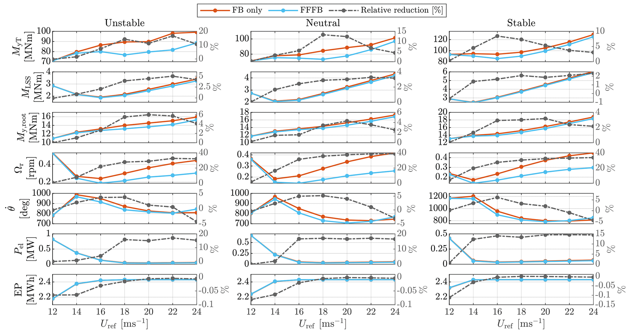
Figure 13Comparison of DEL (MyT, MLSS, My,root), SD (Ωr, , Pel), and EP, simulated using the Mann model. Note that the value of the relative reduction are reflected by the right-side y axis. Relative reduction: (FB-only–FFFB)/(FB-only).
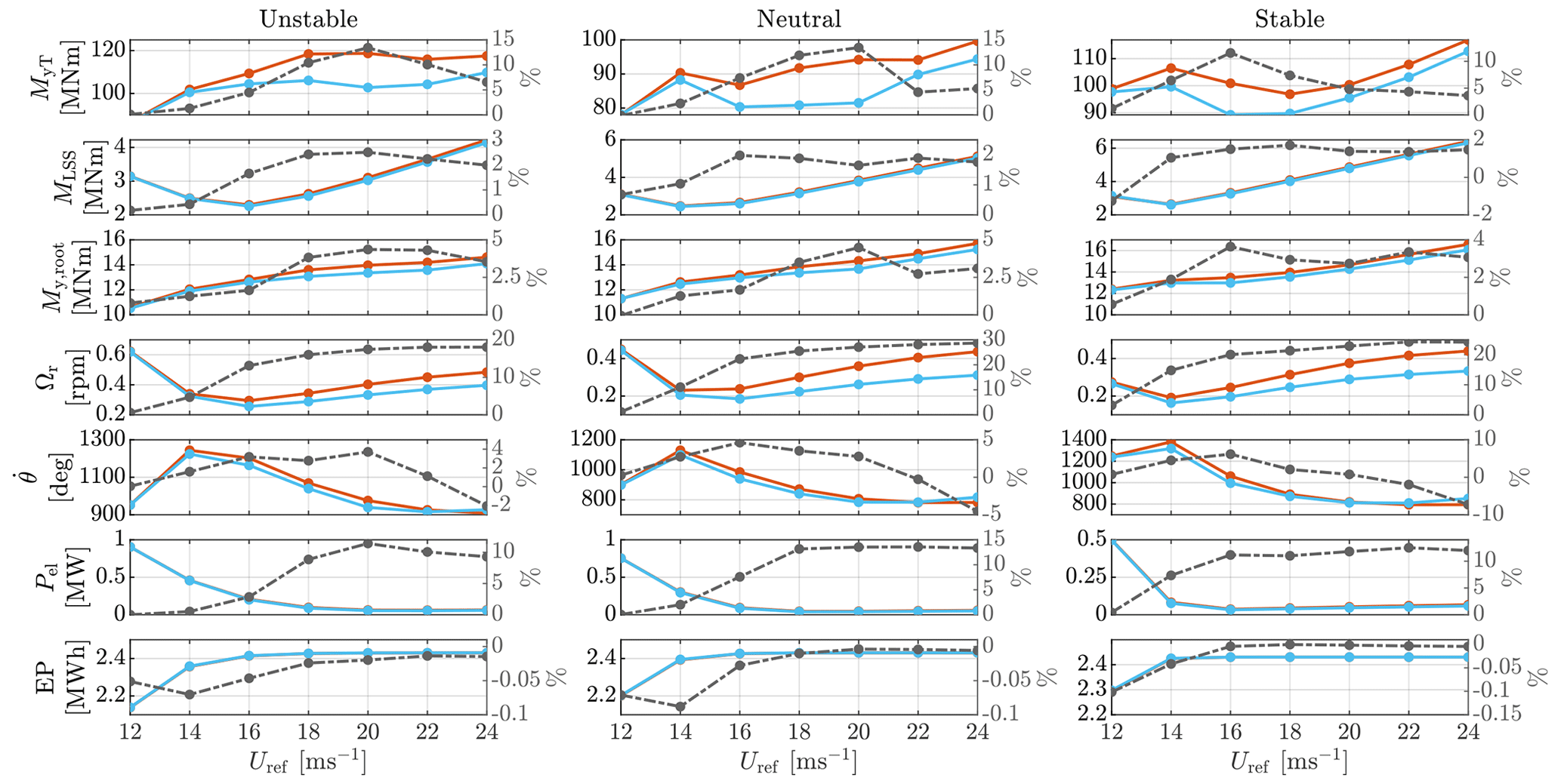
Figure 14Comparison of DEL (MyT, MLSS, My,root), SD (Ωr, , Pel), and EP, simulated using the Kaimal model. Note that the value of the relative reduction are reflected by the right-side y axis. Relative reduction: (FB-only–FFFB)/(FB-only).
Mann-model-based results
Figure 13 compares the DEL, standard deviation (SD), and energy production (EP) results by the Mann model. The relative reductions (see the figure caption) between FB-only and FFFB controls are plotted by the grey lines.
There are overall obvious reductions of the tower fore–aft bending moment DEL in all the investigated atmospheric stability classes. The largest reduction is found to be 16.7 % by a mean wind speed of 22 m s−1 and under an unstable atmosphere. In the unstable case, it can be seen that the reduction is more clear with a higher wind speed. On the opposite, for the stable stability, the reduction is larger at 16 and 18 m s−1, and it reduces as wind speed increases. As for the neutral case, the benefits are the greatest close to 18 m s−1. However, with the mean wind speeds below 14 m s−1 and in the unstable and neutral cases, the FFFB benefits become marginal. This can be caused by a higher possibility to pass the wind speed range where the feedforward pitch is inactivated, as discussed in Sect. 4.4.
As for the low-speed shaft torque, the DEL is reduced by more than 4.0 % under the unstable case for wind speed above 18 m s−1. In addition, the reduction is about 1.5 %–3.3 % and 1.4 %– 2.3 % under neutral and stable cases, respectively.
The DEL of the blade out-of-plane moment is reduced by introducing LAC. More benefits (about 2.7 %–6.0 %) are found under the unstable case. In the neutral stability, the reduction is better at 20 m s−1, where the value is close to 4.3 %, and it drops to 2.5 % by higher wind speeds and to 1.3 % by lower wind speeds. As for stable atmosphere, the reduction is more obvious (around 3.0 %) at wind speeds between 16 and 20 m s−1.
The SD of rotor speed is found to be reduced significantly using FFFB control. The reductions are more than 20 % and up to 40 %. Also, it can be seen that the reductions are more significant under higher mean wind speeds, which is similar in all the three atmosphere stability classes.
Introduction of the FF pitch also generally helps to reduce the standard deviation of pitch rate (speed) . Among the three stability classes, the standard deviations of pitch rate are reduced clearly (varying from 2.0 % to 6.1 %) from 14 to 20 m s−1. However, the reduction stops at the mean wind of 24 m s−1 for unstable and neutral conditions. In the stable atmosphere, the pitch rate SD only reduces with mean wind speeds smaller than 20 m s−1.
As for the electrical power SD, it is reduced obviously by about 16 % in the unstable case for wind speed above 18 m s−1, by about 17 % in the neutral case for wind speed above 16 m s−1, and by 13 % in the stable case for wind speed above 14 m s−1.
With the same mean wind speed but under different stability cases, the electricity productions are similar either using LAC or not. For all the stability conditions, the electricity productions are lower at wind speeds below 14 m s−1 because there is a higher probability that the REWS goes below the rated value, and the electrical power does not reach the rated power.
Kaimal-model-based results
The results using the Kaimal model are shown in Fig. 14. Generally, under different stability classes and mean wind speeds, the statistics show a similar trend to the results obtained by the Mann model. However, the values show some differences.
In terms of tower fore–aft bending moment, the reductions of DEL are from 10.4 % to 13.4 % with a mean wind speed from 18 to 20 m s−1 under unstable and neutral conditions. In the stable case, the reduction is close to 11.5 %, with the mean wind speed of 16 m s−1, and it drops with the higher mean wind speeds.
The results of low-speed shaft DEL show a similar trend to that using the Mann model. On average, for wind speed above 16 m s−1, the shaft load is reduced by around 2.3 %, 1.9 %, and 1.7 %, respectively, under the three investigated stability classes.
Generally, the reduction of the blade root load simulated using the Kaimal model is similar to that based on the Mann model. On average, for wind speed above 16 m s−1, the blade root DEL is reduced by around 4.1 %, 3.0 %, and 3.0 %, respectively, under the three investigated stability classes.
The SD of rotor speed is found to be reduced obviously using FFFB control. The reductions are more than 15 % and are up to 30 %. The result shows a similar trend to that of the Mann-model-based result. However, we can also see the reduction is less than that shown by the Mann model.
The pitch actions show high similarity with that simulated using the Mann model. At mean wind speeds from 16 to 20 m s−1, the reductions in pitch rate SD are about 3.0 % to 3.5 % under unstable and neutral stability classes, and they become less in other mean wind speeds. For the stable case, the reduction is higher at 16 m s−1, reaching 6.2 %, but decreases rapidly as the mean wind speed increases. For very high mean wind speeds above 22 m s−1, the pitch rate SD is increased using LAC.
Since the variation in electrical power is highly linked with the rotor speed, the reductions in the SD of power lie around 10 %, 13 %, and 11 %, respectively, under the three investigated stability classes. These values are smaller than those observed using the Mann model.
The electricity production shows very similar results to those simulated by the Mann model. Using LAC has a marginal impact on electricity production.
In general, the benefits of LAC in load reduction by a four-beam lidar are clear. However, we also show that there are some uncertainties and differences when assessing LAC by different IEC turbulence models. Among the compared turbine loads, LAC has the most significant load reduction effect in the tower base fore–aft bending moment. There are also considerable reductions in speed and power variations. The electrical power generation is not significantly affected by introducing LAC. The load reductions also show differently under different turbulence parameters represented by different atmosphere stability classes. For different stability conditions but the same mean wind speed, it can be seen that the LAC benefits for the load reduction are overall highest in the unstable, medium in neutral, and lowest in stable atmospheric classes. The reason could be the difference in turbulence length scales. The turbulence length scale is lower under a stable condition, which means the peak of the turbulence spectrum appears at a higher wavenumber/frequency (based on the conversion ). The turbine's structural loads are mainly excited by frequency above 0.1 Hz, e.g., the tower natural frequency, the shaft natural frequency (above 1 Hz), the 1 p frequency, and the 3 p (three times per rotation) frequency. If the spectrum has a higher peak frequency, the load will be more dominated by the higher-frequency parts due to the higher excitation of the natural modes. Then the LAC benefits become less significant because it mainly reduces the loads below 0.1 Hz (for the lidar and turbine we used). When considering different mean wind speeds, the discussions above indicate that a higher mean wind speed shifts the spectral peak frequency to be a higher value; therefore, the LAC benefits become less. For the stable condition, the spectral peak frequency is naturally high due to the smaller turbulence length scale, so it is more sensitive to the changes in the mean wind speed. For unstable and neutral cases, the spectrum peak frequency is naturally lower than that in the stable condition; thus the LAC benefits do not decrease as fast as that in the stable condition.
This paper evaluates lidar-assisted wind turbine control under various turbulence characteristics using a four-beam liar and the NREL 5.0 MW reference turbine. The main contributions of this work include (a) summarizing the turbulence spectra and the coherence under various atmosphere stability conditions, (b) analyzing the requirement of filter design for lidar-assisted wind turbine control under various turbulence characteristics, (c) developing a reference lidar-assisted control package, and (d) evaluating the benefits of lidar-assisted wind turbine control using two turbulence models through aeroelastic simulations.
Currently, two turbulence models (the Mann model and the Kaimal model) are provided by the IEC standard for turbine aeroelastic simulation. The recent research has made it possible to generate 4D stochastic turbulence fields in aeroelastic simulation for both the Mann model and the Kaimal model, which allows for simulating lidar measurements more realistically and assessing the potential benefits by lidar-assisted control more reasonably. When evaluating the benefits of lidar-assisted control, previous research uses the Kaimal model with fixed-turbulence spectral parameters provided by the IEC standard (Schlipf, 2015). Thus, the variations of turbulence characteristics by atmospheric stability have not been considered. In this study, we defined three turbulence cases whose characteristics are summarized from unstable, neutral, and stable atmospheric stability conditions. The turbulence spectrum and spatial coherence with separations in all directions are derived.
Based on the defined three turbulence cases, we analyzed the coherence between the rotor-effective wind speed and the one estimated by lidar. The NREL 5.0 MW reference wind turbine and a four-beam pulsed lidar system are taken into consideration. It is found that some differences appear between the results of the Mann model and that of the Kaimal model. The coherence using the Mann model is generally higher in all atmospheric stability classes than the coherence using the Kaimal model. We further analyzed the optimal transfer function, which is important to design a filter that removes the uncorrelated content in the lidar-estimated rotor-effective wind speed signal for lidar-assisted control. For most of the above-rated wind speeds, the analysis revealed that the difference for the transfer function between using different turbulence models or different stability classes is not very significant. This also means a simple linear filter design for lidar-assisted control is sufficient for various atmospheric stability conditions. However, for wind speed above 20 m s−1, the cutoff frequency of unstable condition is about 0.02 Hz higher than that in the neutral stability. The non-ideal filtering should be further analyzed, which is caused by using the cutoff frequency derived from neutral stability for unstable stability. Also, the conclusions in this paragraph may not be applied to turbines of other sizes and lidars with other trajectories. The analysis of coherence and transfer function study can be extended for larger rotor turbines and other lidars with different trajectories.
To further analyze the impact of atmospheric stability for lidar-assisted control, a reference lidar-assisted control package is developed and used in this work. The lidar-assisted control package includes several DLL modules written in FORTRAN: (1) a wrapper DLL that calls all sub-DLLs sequentially, (2) the lidar data processing DLL that estimates the REWS and records the leading time of the REWS, (3) a feedforward pitch module that filters the REWS and activates the feedforward rate at the correct time, and (4) a modified reference FB controller (ROSCO) which can receive a feedforward command.
The benefits of lidar-assisted control are evaluated using both the Mann model and the Kaimal-model-based 4D turbulence. The simulations are performed for the mean wind speed level from 12 to 24 m s−1, using the NREL 5.0 MW reference wind turbine and a four-beam lidar system. For the results with the Mann model, using lidar-assisted control reduces the variations in rotor speed, blade pitch rate, and electrical power significantly. Among the three investigated stability classes and above the mean wind speed of 16 m s−1, the load reductions for the tower bending moment, blade root bending moment, and low-speed shaft torque are observed to be approximately 3.0 % to 16.7 %, 1.5 % to 6.0 %, and 1.7 % to 5.0 %, respectively. The greatest potential of lidar-assisted control in load reduction is found in the tower base loads, and the benefits are found to vary by turbulence spectral properties and mean wind speeds. For the results of the Kaimal model, using lidar-assisted control also clearly reduces the variation in rotor speed, blade pitch rate, and electrical power. The load reduction of the tower bending moment is found in all stability classes for wind speed above 16 m s−1, and it varies from 3.6 % to 13.4 %. The load reduction for the blade root bending moment is between 1.6 % to 4.5 % and for the low-speed shaft torque between 1.6 % to 2.5 %. Besides, with the help of lidar-assisted control, for both turbulence models, the standard deviation of pitch rate (speed) can be reduced (up to 6 %,) for most of the mean wind speed range (below 20 m s−1) and for all stability classes. The pitch rate standard deviation reduction can bring potential load alleviation for the pitch bearings and gears. Overall, we found the benefits of lidar-assisted control by the Kaimal model are slightly different from the results obtained using the Mann model. The benefits of lidar-assisted control simulated using the Mann model are slightly better than those using the Kaimal model, which can be caused by differences in the turbulence spatial coherence between the two models. The lidar preview quality modeled using the Mann model is generally superior to that modeled using the Kaimal model. For both turbulence models, there are clear trends that the benefits of lidar-assisted control in load reduction are the highest in unstable stability, medium in neutral stability, and lowest in a stable atmosphere.
With this work, we show that the mean wind speed, the turbulence spectrum, coherence, and the used turbulence models all have certain impacts on the results of evaluating lidar-assisted control. In this paper, the same turbulence intensity level is assumed for different atmospheric conditions. However, in reality, the turbulence intensity depends on the stability conditions of the atmosphere. In the future, we recommend assessing the benefits of lidar-assisted control depending on site-specific turbulence characteristics and statistics. Also, it is necessary to consider the uncertainties in turbulence models when performing load analysis using aeroelastic simulations.
The OpenFASTv3.0 version with a lidar simulator integrated can be accessed via https://github.com/MSCA-LIKE/OpenFAST3.0_Lidarsim (last access: 1 February 2023; https://doi.org/10.5281/zenodo.7594971, fengguoFUAS, 2023a). The 4D Mann turbulence generator can be found by https://github.com/MSCA-LIKE/4D-Mann-Turbulence-Generator (last access: 1 February 2023; https://doi.org/10.5281/zenodo.7594951, fengguoFUAS, 2023b). The source codes of the wrapper DLL, baseline lidar data processing DLL, pitch feedforward DLL, and modified ROSCO DLL are all available from https://github.com/MSCA-LIKE/Baseline-Lidar-assisted-Controller (last access: 1 February 2023; https://doi.org/10.5281/zenodo.7594961, fengguoFUAS, 2023c).
Simulation data of this paper are available upon request from the corresponding author.
FG conceived the concept, performed the simulations, and prepared the paper. DS supported by verifying the simulations, provided general guidance, and reviewed the paper. PWC provided suggestions and revised and reviewed the paper.
The contact author has declared that none of the authors has any competing interests.
Publisher’s note: Copernicus Publications remains neutral with regard to jurisdictional claims in published maps and institutional affiliations.
This research received financial support from the European Union's Horizon 2020 research and innovation program under the Marie Skłodowska-Curie grant agreement no. 858358 (LIKE – Lidar Knowledge Europe).
This research has been supported by the European Commission, Horizon 2020 Framework Programme (LIKE (grant no. 858358)).
This paper was edited by Jan-Willem van Wingerden and reviewed by Eric Simley and one anonymous referee.
Abbas, N. J., Zalkind, D. S., Pao, L., and Wright, A.: A reference open-source controller for fixed and floating offshore wind turbines, Wind Energ. Sci., 7, 53–73, https://doi.org/10.5194/wes-7-53-2022, 2022. a, b, c, d
Bossanyi, E. A., Kumar, A., and Hugues-Salas, O.: Wind turbine control applications of turbine-mounted LIDAR, J. Phys.-Conf. Ser., 555, 012011, https://doi.org/10.1088/1742-6596/555/1/012011, 2014. a
Chen, Y., Schlipf, D., and Cheng, P. W.: Parameterization of wind evolution using lidar, Wind Energ. Sci., 6, 61–91, https://doi.org/10.5194/wes-6-61-2021, 2021. a, b, c
Chen, Y., Guo, F., Schlipf, D., and Cheng, P. W.: Four-dimensional wind field generation for the aeroelastic simulation of wind turbines with lidars, Wind Energ. Sci., 7, 539–558, https://doi.org/10.5194/wes-7-539-2022, 2022. a, b, c, d, e, f, g
Chen, Z. and Stol, K.: An assessment of the effectiveness of individual pitch control on upscaled wind turbines, J. Phys.-Conf. Ser., 524, 012045, https://doi.org/10.1088/1742-6596/524/1/012045, 2014. a
Cheynet, E., Jakobsen, J. B., and Obhrai, C.: Spectral characteristics of surface-layer turbulence in the North Sea, Energ. Proced., 137, 414–427, https://doi.org/10.1016/j.egypro.2017.10.366, 2017. a
Davenport, A. G.: The spectrum of horizontal gustiness near the ground in high winds, Q. J. Roy. Meteor. Soc., 87, 194–211, https://doi.org/10.1002/qj.49708737208, 1961. a
Davoust, S. and von Terzi, D.: Analysis of wind coherence in the longitudinal direction using turbine mounted lidar, J. Phys.-Conf. Ser., 753, 072005, https://doi.org/10.1088/1742-6596/753/7/072005, 2016. a
DNV-GL: Bladed theory manual: version 4.8, Tech. rep., Garrad Hassan & Partners Ltd., Bristol, UK, 2016. a
Dong, L., Lio, W. H., and Simley, E.: On turbulence models and lidar measurements for wind turbine control, Wind Energ. Sci., 6, 1491–1500, https://doi.org/10.5194/wes-6-1491-2021, 2021. a, b, c
Dunne, F., Schlipf, D., Pao, L., Wright, A., Jonkman, B., Kelley, N., and Simley, E.: Comparison of two independent lidar-based pitch control designs, in: 50th AIAA Aerospace Sciences Meeting Including the New Horizons Forum and Aerospace Exposition, Nashville, Tennessee, January 2012, https://www.osti.gov/biblio/1047948 (last access: 1 Februrary 2023), p. 1151, 2012. a
fengguoFUAS: MSCA-LIKE/OpenFAST3.0_Lidarsim: OpenFAST3.0_Lidarsim (OpenFAST3.0_Lidarsim_v1), Zenodo [code], https://doi.org/10.5281/zenodo.7594971, 2023a. a
fengguoFUAS: MSCA-LIKE/4D-Mann-Turbulence-Generator: 4D-Mann-Turbulence-Generator (4D_MannTurbulence_v1), Zenodo [code], https://doi.org/10.5281/zenodo.7594951, 2023b. a
fengguoFUAS: MSCA-LIKE/Baseline-Lidar-assisted-Controller: Baseline-Lidar-assisted-Controller (Baseline-Lidar-assisted-Controllerv_1), Zenodo [code], https://doi.org/10.5281/zenodo.7594961, 2023c. a
Guo, F., Mann, J., Peña, A., Schlipf, D., and Cheng, P. W.: The space-time structure of turbulence for lidar-assisted wind turbine control, Renew. Energ., 195, 293–310, https://doi.org/10.1016/j.renene.2022.05.133, 2022a. a, b, c, d, e, f, g, h, i, j, k, l, m, n, o, p, q
Guo, F., Schlipf, D., Zhu, H., Platt, A., Cheng, P. W., and Thomas, F.: Updates on the OpenFAST Lidar Simulator, J. Phys.-Conf. Ser., 2265, 042030, https://doi.org/10.1088/1742-6596/2265/4/042030, 2022b. a, b, c, d, e, f
Held, D. P. and Mann, J.: Lidar estimation of rotor-effective wind speed – an experimental comparison, Wind Energ. Sci., 4, 421–438, https://doi.org/10.5194/wes-4-421-2019, 2019. a, b, c, d, e, f, g, h
Hunt, J. C. and Carruthers, D. J.: Rapid distortion theory and the “problems” of turbulence, J. Fluid Mech., 212, 497–532, https://doi.org/10.1017/S0022112090002075, 1990. a
IEC 61400-1:2019: Wind energy generation systems – Part 1: Design requirements, Standard, International Electrotechnical Commission, Geneva, Switzerland, 2019. a, b, c, d, e, f, g, h, i, j, k, l
Jones, B. L., Lio, W., and Rossiter, J.: Overcoming fundamental limitations of wind turbine individual blade pitch control with inflow sensors, Wind Energy, 21, 922–936, https://doi.org/10.1002/we.2205, 2018. a
Jonkman, B. J.: TurbSim user's guide: Version 1.50, Tech. rep., National Renewable Energy Lab. (NREL), Golden, CO (United States), https://doi.org/10.2172/965520, 2009. a
Jonkman, J. and Buhl, M. L.: FAST User's Guide, Tech. Rep. EL-500-38230, NREL, https://doi.org/10.2172/15020796, 2005. a
Jonkman, J., Butterfield, S., Musial, W., and Scott, G.: Definition of a 5-MW reference wind turbine for offshore system development, Tech. rep., National Renewable Energy Lab. (NREL), Golden, CO (United States), https://doi.org/10.2172/947422, 2009. a, b, c
Julier, S. J. and Uhlmann, J. K.: Unscented filtering and nonlinear estimation, P. IEEE, 92, 401–422, https://doi.org/10.1109/JPROC.2003.823141, 2004. a
Kaimal, J. C., Wyngaard, J. C., Izumi, Y., and Coté, O. R.: Spectral characteristics of surface-layer turbulence, Q. J. Roy. Meteor. Soc., 98, 563–589, https://doi.org/10.1002/qj.49709841707, 1972. a, b
Laks, J., Simley, E., and Pao, L.: A spectral model for evaluating the effect of wind evolution on wind turbine preview control, in: 2013 American Control Conference,Washington, DC, USA, 17–19 June 2013, IEEE, 3673–3679, https://doi.org/10.1109/ACC.2013.6580400, 2013. a
Lee, K., Shin, H., and Bak, Y.: Control of Power Electronic Converters and Systems, Academic Press, 392 pp., https://doi.org/10.1016/C2015-0-02427-3, 2018. a
Mann, J.: The spatial structure of neutral atmospheric surface-layer turbulence, J. Fluid Mech., 273, 141–168, https://doi.org/10.1017/S0022112094001886, 1994. a, b, c, d, e, f, g, h
Mann, J.: Wind field simulation, Probabilist. Eng. Mech., 13, 269–282, https://doi.org/10.1016/S0266-8920(97)00036-2, 1998. a, b, c
Mann, J., Cariou, J.-P. C., Parmentier, R. M., Wagner, R., Lindelöw, P., Sjöholm, M., and Enevoldsen, K.: Comparison of 3D turbulence measurements using three staring wind lidars and a sonic anemometer, Meteorol. Z., 18, 135–140, https://doi.org/10.1127/0941-2948/2009/0370, 2009. a
Matsuishi, M. and Endo, T.: Fatigue of metals subjected to varying stress, Japan Society of Mechanical Engineers, Fukuoka, Japan, 68, 37–40, 1968. a
Mirzaei, M. and Mann, J.: Lidar configurations for wind turbine control, J. Phys.-Conf. Ser., 753, 032019, https://doi.org/10.1088/1742-6596/753/3/032019, 2016. a, b, c
NREL: OpenFAST Documentation, Tech. Rep. Release v3.3.0, National Renewable Energy Laboratory, https://openfast.readthedocs.io/en/main/ (last access: 1 January 2023), 2022. a
Nybø, A., Nielsen, F. G., Reuder, J., Churchfield, M. J., and Godvik, M.: Evaluation of different wind fields for the investigation of the dynamic response of offshore wind turbines, Wind Energy, 23, 1810–1830, https://doi.org/10.1002/we.2518, 2020. a
Peña, A., Mann, J., and Dimitrov, N.: Turbulence characterization from a forward-looking nacelle lidar, Wind Energ. Sci., 2, 133–152, https://doi.org/10.5194/wes-2-133-2017, 2017. a, b
Peña, A.: Østerild: A natural laboratory for atmospheric turbulence, J. Renew. Sustain. Ener., 11, 063302, https://doi.org/10.1063/1.5121486, 2019. a, b, c, d, e
Peña, A., Hasager, C. B., Lange, J., Anger, J., Badger, M., and Bingöl, F.: Remote Sensing for Wind Energy, Tech. Rep. DTU Wind Energy-E-Report-0029(EN), DTU Wind Energy, Roskilde, Denmark, https://orbit.dtu.dk/files/55501125/Remote_Sensing_for_Wind_Energy.pdf (last access: 1 February 2023), 2013. a
Schlipf, D.: Lidar-Assisted Control Concepts for Wind Turbines, Dissertation, University of Stuttgart, https://doi.org/10.18419/opus-8796, 2015. a, b, c, d, e, f, g, h, i, j, k, l, m, n, o, p, q, r, s
Schlipf, D., Cheng, P. W., and Mann, J.: Model of the Correlation between Lidar Systems and Wind Turbines for Lidar-Assisted Control, J. Atmos. Ocean. Tech., 30, 2233–2240, https://doi.org/10.1175/JTECH-D-13-00077.1, 2013a. a, b, c
Schlipf, D., Schlipf, D. J., and Kühn, M.: Nonlinear model predictive control of wind turbines using LIDAR, Wind Energy, 16, 1107–1129, https://doi.org/10.1002/we.1533, 2013b. a
Schlipf, D., Fürst, H., Raach, S., and Haizmann, F.: Systems Engineering for Lidar-Assisted Control: A Sequential Approach, J. Phys.-Conf. Ser., 1102, 012014, https://doi.org/10.1088/1742-6596/1102/1/012014, 2018a. a, b
Schlipf, D., Hille, N., Raach, S., Scholbrock, A., and Simley, E.: IEA Wind Task 32: Best Practices for the Certification of Lidar-Assisted Control Applications, J. Phys.-Conf. Ser., 1102, 012010, https://doi.org/10.1088/1742-6596/1102/1/012010, 2018b. a
Schlipf, D., Lemmer, F., and Raach, S.: Multi-variable feedforward control for floating wind turbines using lidar, in: The 30th International Ocean and Polar Engineering Conference, OnePetro, Virtual, 11–16 October 2020, https://doi.org/10.18419/opus-11067, 2020. a
Shan, M.: Load Reducing Control for Wind Turbines: Load Estimation and Higher Level Controller Tuning based on Disturbance Spectra and Linear Models, PhD thesis, Kassel, Universität Kassel, Fachbereich Elektrotechnik/Informatik, https://kobra.uni-kassel.de/handle/123456789/2017050852519 (last access: 1 February 2023), 2017. a
Simley, E.: Wind Speed Preview Measurement and Estimation for Feedforward Control of Wind Turbines, ProQuest Dissertations & Theses, Ann Arbor, https://www.proquest.com/docview/1719284807 (last access: 1 February 2023), 2015. a, b
Simley, E. and Pao, L.: Reducing LIDAR wind speed measurement error with optimal filtering, in: 2013 American Control Conference, Washington, DC, USA, 17–19 June 2013, 621–627, https://doi.org/10.1109/ACC.2013.6579906, 2013. a, b, c
Simley, E. and Pao, L.: A longitudinal spatial coherence model for wind evolution based on large-eddy simulation, in: 2015 American Control Conference (ACC), IEEE, Chicago, IL, USA, 1–3 July 2015, 3708–3714, https://doi.org/10.1109/ACC.2015.7171906, 2015. a, b, c, d, e, f, g
Simley, E., Fürst, H., Haizmann, F., and Schlipf, D.: Optimizing Lidars for Wind Turbine Control Applications – Results from the IEA Wind Task 32 Workshop, Remote Sensing, 10, 863, https://doi.org/10.3390/rs10060863, 2018. a, b, c, d
Stammler, M., Schwack, F., Bader, N., Reuter, A., and Poll, G.: Friction torque of wind-turbine pitch bearings – comparison of experimental results with available models, Wind Energ. Sci., 3, 97–105, https://doi.org/10.5194/wes-3-97-2018, 2018. a
Taylor, G. I.: The spectrum of turbulence, P. R. Soc. A, 164, 476–490, https://doi.org/10.1098/rspa.1938.0032, 1938. a, b, c, d, e
von Kármán, T.: Progress in the statistical theory of turbulence, P. Natl. Acad. Sci. USA, 34, 530, https://doi.org/10.1073/pnas.34.11.530, 1948. a
Welch, P.: The use of fast Fourier transform for the estimation of power spectra: a method based on time averaging over short, modified periodograms, IEEE Trans. Audio, 15, 70–73, https://doi.org/10.1109/TAU.1967.1161901, 1967. a, b
Wiener, N.: Extrapolation, interpolation, and smoothing of stationary time series: with engineering applications, vol. 8, MIT press Cambridge, MA, ISBN 9780262730051, 1964. a
- Abstract
- Introduction
- Turbulence modeling
- Correlation between lidars and turbines
- Lidar-assisted controller design
- Simulation, results, and discussion
- Conclusions
- Code availability
- Data availability
- Author contributions
- Competing interests
- Disclaimer
- Acknowledgements
- Financial support
- Review statement
- References