A new base of wind turbine noise measurement data and its application for a systematic validation of sound propagation models

Extensive measurements in the area of wind turbines were performed in order to validate a sound propagation model which is based on the Crank–Nicolson parabolic equation method. The measurements were carried out over a flat grass-covered landscape and under various environmental conditions. During the measurements, meteorological and wind turbine performance data were acquired and acoustical data sets were recorded at distances of 178, 535 and 845 m from the wind turbine. By processing and analysing the measurement data, validation cases and input parameters for the sound propagation model were derived. The validation includes five groups that are characterised by different sound propagation directions, i.e. downwind, crosswind and upwind conditions in varying strength. In strong upwind situations, the sound pressure levels at larger distances are overestimated because turbulence is not considered in the modelling. In the other directions, the model reproduces the measured sound propagation losses well in the overall sound pressure level and in the third octave band spectra. As in the recorded measurements, frequency-dependent maxima and minima are identified, and losses generally increase with increasing distance and frequency. The agreement between measured and modelled sound propagation losses decreases with distance. The data sets used in the validation are freely accessible for further research.

1 Introduction

From 2009 to 2020, the global capacity of onshore wind turbines increased from 157 to 707 GW. Further growth of 399 GW is expected in the years 2021 to 2025 (Lee and Zhao, 2021). With the expansion of wind energy and the decreased distance between turbines and local residents, the noise emission from wind turbines and its propagation have come into focus. This paper addresses the latter issue – the sound propagation of wind turbines.

Various analytical and numerical modelling techniques have been applied to predict the outdoor noise propagation (Bérengier et al., 2003). The most well-known physically based sound propagation models are the ray-tracing and the parabolic equation (PE) methods. With a focus on low-level sources, most of the models are verified using the benchmark of Attenborough et al. (1995) and are partially validated with measured data. Performing and evaluating acoustic measurements requires a lot of effort and cost, especially for high-level sources such as wind turbines. As a result, numerical models for high-level sources have often been verified by analytical results (e.g. Lee et al., 2016; Cotté, 2019) or engineering models (e.g. Bolin and Boué, 2009; Kaliski and Wilson, 2011) in the past but are less validated by measured data.

In addition to analytical solutions, Lee et al. (2016) compared numerical results with far-field acoustic measurements to validate the PE method. For this, two loudspeakers were placed at 20 and 80 m height on a meteorological mast, and seven microphones were positioned at 2 m height and at a 500 to 1700 m distance from the mast. Single tone frequencies (125, 250, 500 and 1000 Hz) were used as sources. In the downwind direction, good agreement between measurements and the model was observed for both speaker heights. Since no turbulence was taken into account in the model, the sound level in the upwind direction was greatly overestimated by the PE method.

Shen et al. (2020) carried out measurements with a loudspeaker including the detection of fluid and acoustic quantities to validate four different propagation models, namely the PE-based WindSTAR (Barlas et al., 2017a) and the ray-tracing-based Nord2000 (Plovsing, 2014), as well as the ISO 9613-2 (1996) and DK-BEK513 (2019) standards. The loudspeaker was placed at a height of 109 m, the atmospheric conditions were recorded by a meteorological mast and the acoustic measurements were performed with 11 microphones placed at different distances to the turbine. White noise and band-limited white noise were applied as signals. For two different wind shears, the measured and modelled one-third octave spectra (125 to 1000 Hz) were compared and the average difference of the overall sound pressure level was determined. Depending on the microphone position and propagation model, the difference of measured and modelled data was between −3.43 and 2.45 dB. The comparison was performed for one wind direction.

In Prospathopoulos and Voutsinas (2005), a sound propagation model based on ray tracing was validated by acoustic measurements in the area of one wind turbine. For this purpose, the sound pressure level was recorded somewhere between 70 and 88 m and at a 530 m distance from the turbine. Validating the model, the measured and modelled propagation losses between $\mathrm{70}/\mathrm{88}$ and 530 m were compared in one-third octave bands. Using one scenario as an example, i.e. for downwind conditions and flat land, good agreement was shown. However, as the focus of the paper was the investigation of different propagation effects, no further validation cases were presented. Moreover, with a hub height of 60 m, the investigated wind turbine does not correspond to the current scales, which are typically between 80 and 120 m.

As part of the project “Noise and energy optimisation of wind farms”, extensive measurements were carried out to validate the Nord2000 propagation model for the use of wind turbine noise (Søndergaard and Plovsing, 2009). This ray-tracing-based model was validated by several field measurements with different sources – namely with two loudspeakers, a single wind turbine and a whole wind farm. Data from a 100 m meteorological mast were used to determine sound speed profiles. In general, good agreements were obtained for simple and also complex conditions regarding meteorology and landscape. For the loudspeaker test in flat terrain, distances of up to 1500 m were considered. Showing an average deviation of 0.1 dB and a standard deviation of 0.7 dB, very good results were achieved in the downwind direction. With an average deviation of 4.3 dB and a standard deviation of 1.9 dB, higher differences of measured and modelled data were examined in the upwind direction. Herein, the predicted propagation losses were 4 dB lower than the measured ones. Note that turbulence constants were taken into account in the model. For the validation with a single wind turbine, only downwind conditions were considered. The results show differences between −3.8 and 1.3 dB, which correspond to an average deviation of −1.0 dB with a standard deviation of 2.3 dB. Moreover, the measured and predicted one-third octave spectra differ to some extent.

As in Shen et al. (2020), Nyborg et al. (2022) use the sound propagation models ISO 9613-2 (1996), Nord2000 (Plovsing, 2014) and WindSTAR (Barlas et al., 2017a). The models are validated with two data sets derived from loudspeaker and wind turbine measurements. Hereby, measured and modelled one-third octave spectra are compared for three cases with different propagation directions (downwind, crosswind and upwind). The modelled values agree well with the loudspeaker measurements. With increasing frequency, the deviations from the measured values become larger. In comparison with the measured data at a wind turbine, Nord2000 and WindSTAR show good results in the crosswind and upwind directions. Downwind, less good agreements are obtained. In the paper of Nyborg et al. (2022), the modelling of the wind turbine as a sound source is also addressed, as discussed in Sect. 4.1.

For various reasons, the data provided by the literature are not suitable for validating sound propagation models applied to wind turbines. Firstly, loudspeakers do not reflect the spatial and time-dependent sound characteristics of a wind turbine. Second, although atmospheric conditions are often measured, the specific measured values are not available to the reader. Consequently, some of the input parameters for a sound propagation model cannot be derived and the findings cannot be used to validate further models. In order to validate and to improve sound propagation models for wind turbines, open-source measurement data are helpful. For this purpose, a detailed presentation, processing and analysis of the acoustic and meteorological measurement data as well as a subsequent data publication are necessary. For this reason, the objectives of this paper are

1. to introduce comprehensive measurements of acoustic and atmospheric quantities close to a real multi-MW turbine;

2. to prepare, combine and analyse acoustic, atmospheric and wind turbine measurement data for the validation of sound propagation models;

3. to apply prepared data sets for the systematic validation of a numerical sound propagation model based on the PE method, taking into account different propagation directions; and

4. to provide validation data of wind turbine sound propagation for further research purposes.

The paper is structured as follows. In Sect. 2, the methodology is described in detail. The measurements, the PE-based sound propagation model applied and the modelling of a representative sound source of a wind turbine are presented. The focus of the section is in particular on the derivation of input parameters from measurement data for the model. All results are given in Sect. 3. The acoustic and atmospheric measurement data are analysed, and the measurement- and model-based propagation losses are compared using one-third octave bands and total sound pressure levels. Moreover, the validity of model prediction is addressed. In Sect. 4, the results are discussed considering the source model, the impact of ground properties and measurement aspects.

2 Methodology

In this section, an overview of the modelling approach is given first. Then the focus is on the measurements; they are presented in detail, and the derivation of input parameters is discussed extensively. Finally, the validation process is described.

2.1 Modelling

In this work, extensive wind turbine noise measurement data are used to validate a propagation model with a simplified wind turbine sound source. In general, the sound propagation is essentially determined by the geometric attenuation. In addition, sound propagation is influenced by the ground and by atmospheric aspects such as air absorption, refraction and scattering. According to Salomons (2001), the sound pressure level L_p at the place of emission can be calculated as a function of the frequency f:

$$\begin{array}{}\text{(1)}& \begin{array}{rl}{L}_{\mathrm{p}}^n\left(f\right)& =L_W^n\left(f\right)\\ & -\underset{\mathrm{Attenuation}\mathrm{terms}}{\underbrace{\mathrm{10}\cdot \log \mathrm{4}\mathit{\pi }(R^n{)}^{\mathrm{2}}-{\mathit{\alpha }}_L(f)\cdot R^n+\mathrm{\Delta }{L}^n(f)}},\end{array}\end{array}$$

with the sound power level $L_W^n$ of the source n, the distance to the source Rⁿ, the atmospheric air coefficient α_L and the term ΔLⁿ, which describes additional attenuation due to further propagation effects. In this work, the subscript n is also added, referring to the point source number. In Eq. (1), attenuation terms are subtracted from the sound power level. The attenuation terms include the geometrical spreading (first term) and air absorption (second term), which are both dependent on the distance from the source Rⁿ. Furthermore, the air absorption also depends on the atmospheric coefficient α_L, which is calculated as a function of frequency, temperature and humidity according to Bass et al. (1995). The last attenuation term ΔLⁿ describes the sound propagation loss due to ground effects as well as atmospheric refraction and scattering. In this work, ΔLⁿ is determined using the Crank–Nicolson parabolic equation (CNPE) method.

The CNPE method is an efficient methodology for the calculation of sound propagation over large distances, because backscattering is neglected, and the calculations are only performed in the propagation direction (Salomons, 2001). As a result, it is a common approach for predicting the propagation of wind turbine noise (Lee et al., 2016; Barlas et al., 2017a, b; Zhu et al., 2018; Cotté, 2019). The propagation model of this work follows the descriptions in West et al. (1992) and in Salomons (2001) and is shortly introduced in the following. Therefore, the CNPE method is simplified into a two-dimensional form on the basis of an axisymmetric approximation. The two-dimensional Helmholtz equation is given as

$$\begin{array}{}\text{(2)}& {\displaystyle \frac{{\partial }^{\mathrm{2}}q}{\partial r^{\mathrm{2}}}}+{\displaystyle \frac{{\partial }^{\mathrm{2}}q}{\partial z^{\mathrm{2}}}}+k_{\mathrm{eff}}^{\mathrm{2}}\cdot q=\mathrm{0},\end{array}$$

where the sound field q is dependent on the cylindrical coordinates r and z and is associated with the complex pressure amplitude p by $q=p\sqrt{r}$. Moreover, the local effective wavenumber $k_{\mathrm{eff}}=\mathit{\omega }/c_{\mathrm{eff}}$ with the angular frequency ω and the effective sound speed c_eff is considered in Eq. (2). Calculating the sound pressure field q, a wide-angle parabolic equation is solved using the Crank–Nicolson method in the r direction and central finite differences in the z direction. In the simulations of this work, a discretisation equal to $\mathrm{1}/\mathrm{10}$ of the wavelength λ is chosen in both the vertical and horizontal direction (i.e. $\mathrm{\Delta }r=\mathrm{\Delta }z=\mathit{\lambda }/\mathrm{10}$), providing sufficient accuracy. To simulate free-field conditions in the z direction, a perfectly matched layer is used at the upper boundary of the computational domain. The lower boundary is defined by the acoustic ground impedance. For the characterisation of those ground impedances, the Delany–Bazley–Miki model (Miki, 1990) is used accounting for specific ground properties. This model is based on an empirical ground model by Delany and Bazley (1970). Since the site of the measurements was predominantly grass-covered, a flow resistance of 200 kPa s m⁻² is chosen for the Delany–Bazley–Miki model. This, according to various publications, is a typical value for grassland. Moreover, in view of the measurements, a flat terrain is assumed.

The present CNPE model uses a second-order starting field described in Salomons (2001) by

$$\begin{array}{}\text{(3)}& q_{\mathrm{0}}=\sqrt{i{k}_a}(A_{\mathrm{0}}+A_{\mathrm{2}}{k}_a^{\mathrm{2}}{z}^{\mathrm{2}})\exp \left(-{\displaystyle \frac{k_a^{\mathrm{2}}{z}^{\mathrm{2}}}{B}}\right),\end{array}$$

with A₀=1.3717, $A_{\mathrm{2}}=-\mathrm{0.3701}$ and B=3. The starting field represents a monopole sound source.

However, to represent a wind turbine as a source, the approach from Barlas et al. (2017b) is adopted. In this approach the wind turbine is reduced to three point sound sources, which are located at the rotor blade tips, more precisely at 85 % of the rotor length, in the three-dimensional field. According to Oerlemans et al. (2007), the sound radiation of wind turbines is dominant at this position. Transferred to a two-dimensional field, the point sound sources are located at hub height h and at ±85 % of the rotor length l:

$$\begin{array}{}\text{(4)}& h_s=h\pm \mathrm{0.85}l.\end{array}$$

For this simplified representation of a wind turbine, one simulation is performed for each sound source (Barlas et al., 2017b). In the context of this work, the simulation results are subsequently logarithmically summed. As in Nyborg et al. (2022), it is assumed that the point sources are incoherent. Moreover, the sound power level is assumed to be equally distributed among all sources. In this way, the sound power level of the source n is given by

$$\begin{array}{}\text{(5)}& L_W^n=L_W-\mathrm{10}\cdot {\log }_{\mathrm{10}}\left(i\right),\end{array}$$

where i is the total number of sources. As a result of the assumptions, the term of the sound source is cancelled when calculating the sound propagation losses. However, in reality, not all point sources have the same strength, and, in general, the sound propagation loss is only defined for one point source. The method used allows the propagation loss to be adjusted for several point sources and is discussed in Sect. 4.1.

2.2 Measurements

The data sets selected for the validation originate from one of five measurement campaigns, which are described in detail in Martens et al. (2020). In this work, only a very brief overview is given in order to provide the reader with a rough understanding of the measurements. The measurement data used originate from a measurement campaign performed close to a turbine in a wind farm in northern Germany. The landscape of the measurement site is characterised as flat and homogeneous and is predominantly covered with grass. Acoustic and meteorological data as well as turbine-specific parameters of the wind farm, i.e. supervisory control and data acquisition (SCADA) data, were recorded synchronously over a period of several months.

The measurement environment as well as the position of the measurement instruments and turbines are shown in Fig. 1. As can be recognised, several wind turbines are located in the area of the acoustic measurements. It is important to point out that the investigations of this work refer to a single turbine. For validation, only periods where the specific turbine under investigation is on while the surrounding turbines are off are selected.

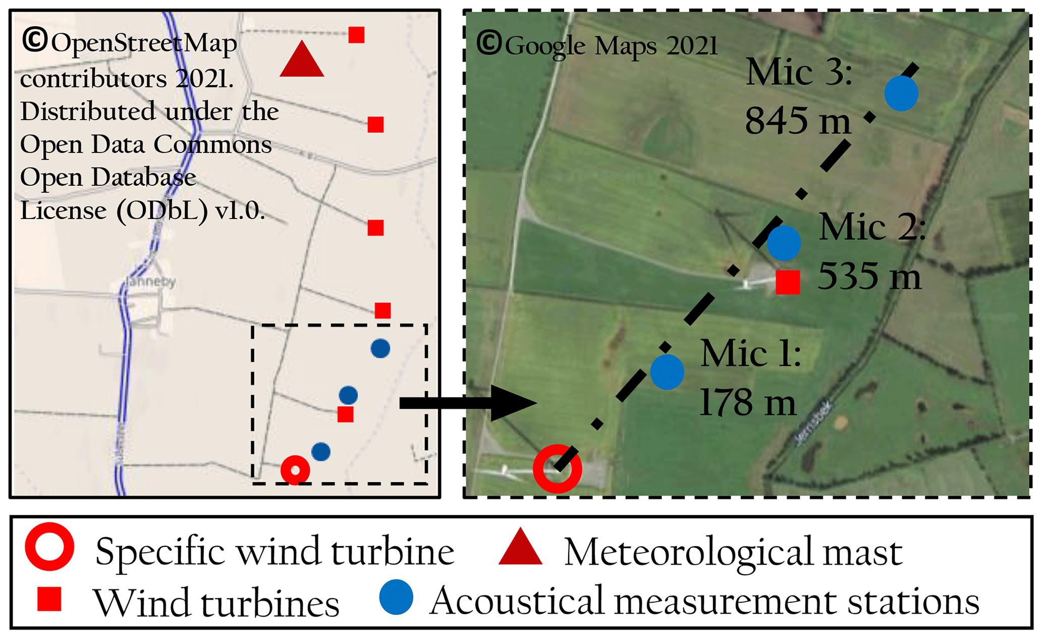
Figure 1 Overview map of the wind farm and detailed measurement plan including the position of a specific wind turbine, acoustical measurement stations and a meteorological mast.

During the campaign, three acoustic measurement stations recorded sound pressure levels, one-third octave bands and audio at a sampling rate of 51 kHz. The distances from the wind turbine to the acoustic stations are summarised in Table 1. To avoid additional extraneous noise from natural sources, the acoustic measurement devices were positioned at least 10 m from possible disturbances. A challenging task for acoustic measurements in the free field is the reduction of wind-induced noise at the microphone. These noises can strongly distort measurement data, especially in the low-frequency range. Using a combination of a nose cone, a 90 mm standard windscreen and an in-house developed 220 mm secondary windscreen, the wind-induced noise at the microphones was effectively reduced during the measurements. The development and further investigations concerning the in-house developed windscreens are described in Martens et al. (2019). An example of an acoustic measurement station with windscreens is shown in Fig. 2. Generally, the height of each sound level meter was 1.70 m. Moreover, the systems were powered by solar panels and an additional external battery during the time of measurements.

Table 1 Horizontal distances from wind turbine to acoustic measurement stations.

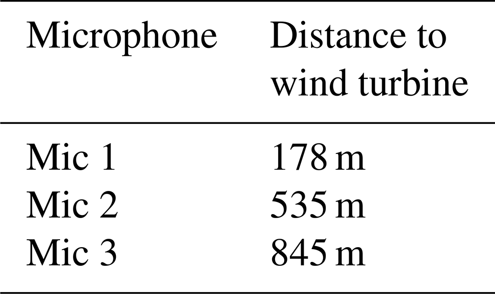
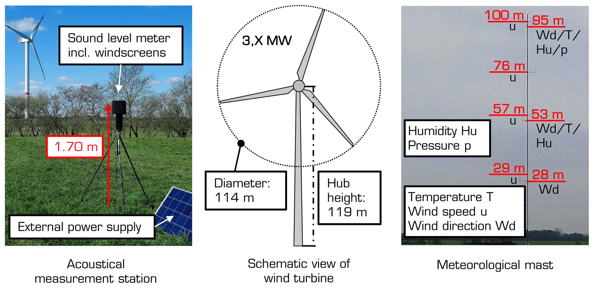
Figure 2 Overview of measurement systems and wind turbine.

Synchronously to the acoustic recordings, extensive meteorological measurements were performed describing the lower atmosphere. A 100 m high measuring mast is permanently positioned in the wind farm, which records temperature and humidity as well as wind speed and wind direction at different heights. These data are available averaged over 10 min. The data of the wind speed are also available at 1 Hz, which is important for the determination of the sound speed profile. The corresponding measurement setup is illustrated in Fig. 2, and the position of the measurement mast is given in Fig. 1. According to this, the meteorological mast is located in the centre of the wind farm. In addition to acoustic and meteorological parameters, the operational data of all wind turbines in the wind farm were detected, such as rotor speed and electrical power. Herein, the data are provided at a resolution of 10 min.

2.3 Determination of input parameters

As mentioned above, sound propagation in the atmosphere is influenced by air absorption, turbulence and atmospheric refraction. The parameters for estimating the air absorption are derived directly from the measurements. Temperature and humidity at 53 m are used to calculate the atmospheric coefficient α_L and, hence, the air absorption using the approach of Bass et al. (1995).

Regarding the atmospheric refraction, the vertical profile of the sound speed is essential. Generally, the sound speed c is calculated by

$$\begin{array}{}\text{(6)}& c_{\mathrm{0}}=\sqrt{\mathit{\kappa }R{T}_{\mathrm{0}}}=\mathrm{20.05}\sqrt{T_{\mathrm{0}}},\end{array}$$

with the specific heat capacity κ set to 1.4 and the gas constant R of dry air to 287 ${\mathrm{Jkg}}^{-\mathrm{1}}{\mathrm{K}}^{-\mathrm{1}}$.

In the moving atmosphere, the speed of sound is superimposed with the prevailing wind speed, which results in the effective sound speed:

$$\begin{array}{}\text{(7)}& c_{\mathrm{eff}}=c_{\mathrm{0}}+u_{\mathrm{comp}}.\end{array}$$

Here, the second term describes the wind component in the sound propagation direction, which is determined using the wind speed u and the angle γ between the wind direction and the sound propagation direction:

$$\begin{array}{}\text{(8)}& u_{\mathrm{comp}}=-\left|u\right|\cdot \cos \left(\mathit{\gamma }\right).\end{array}$$

Consequently, the direction of sound propagation corresponds to the angular relationship between the turbine and the microphones. Note that the sound propagation direction is defined as opposite to the wind direction. The wind direction is the compass direction from which the wind comes. The sound propagation direction is the compass direction in which the sound propagates. Eqs. (6) and (7) are used to calculate the effective sound speed c_eff at the measurement heights illustrated in Fig. 2, i.e. at 29, 57, 76 and 100 m. On the basis of the measured data, it was verified that the wind direction does not change significantly with height (see Sect. 4.3).

However, a high discretisation of the c_eff profile is required for the CNPE method. To determine c_eff from the ground to the maximum height of the computational domain, the log-linear approach introduced in Heimann and Salomons (2004) is followed. Accordingly, at the height z, c_eff can be described as a function of the coefficients a₀, a_log and a_lin and the roughness length z₀ using

$$\begin{array}{}\text{(9)}& c_{\mathrm{eff}}=a_{\mathrm{0}}+a_{\log }\ln {\displaystyle \frac{z+z_{\mathrm{0}}}{z_{\mathrm{0}}}}+a_{\mathrm{lin}}z.\end{array}$$

A value of 0.05 m is chosen as the roughness length, which is considered to be representative of the site according to available turbine reports. The coefficient a₀ corresponds to the speed of sound and is calculated via Eq. (6) using the measured temperature at a height of 53 m. The logarithmic and linear coefficients a_log and a_lin are determined using a pseudo inverse (see Golan, 1995, for foundations).

The accuracy of the fitted vertical profile of c_eff is given by the root mean square error (RMSE) values. A comparison between the original value of c_eff at sensor heights and the estimated vertical profile of the sound speed is shown in Sect. 3.1.

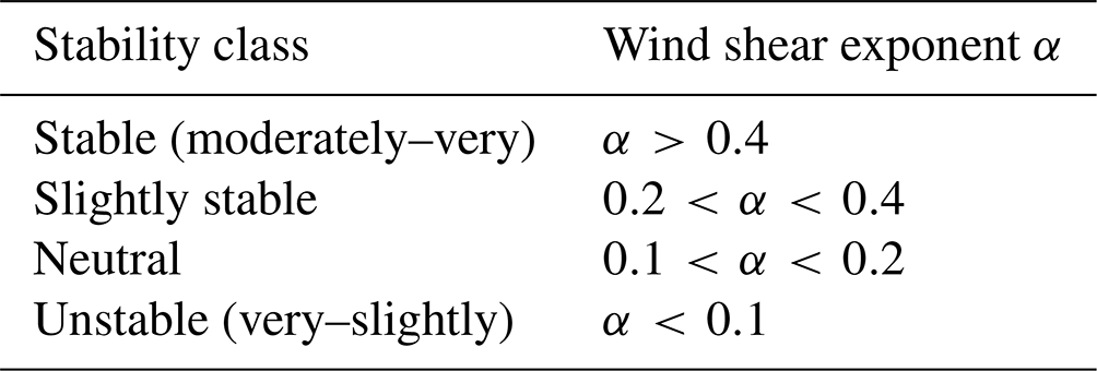
Lately, information on atmospheric stability is needed to classify different propagation conditions and thus to derive diverse validation cases. In this work, the stability conditions are described on the basis of the dimensionless wind shear exponent α. For each 10 min averaging period, α is determined by the power-law expression:

$$\begin{array}{}\text{(10)}& {\displaystyle \frac{u_{z_{\mathrm{2}}}}{u_{z_{\mathrm{1}}}}}={\left({\displaystyle \frac{z_{\mathrm{2}}}{z_{\mathrm{1}}}}\right)}^{\mathit{\alpha }},\end{array}$$

where the mean horizontal wind speeds u in metres per second (m s⁻¹) at the heights z₁ and z₂ are applied. Calculating α, the measured wind speed at z₁=29 and z₂=100 m is used. Subsequently, the stability is divided into the five classes which are specified in many publications (e.g. van den Berg, 2008) and are listed in Table 2.

Table 2 Criteria for stability classes as a function of the wind shear exponent α according to van den Berg (2008).

2.4 Validation procedure

The scheme for validating the sound propagation model with the measurement data is shown in Fig. 3. The procedure is divided into five steps.

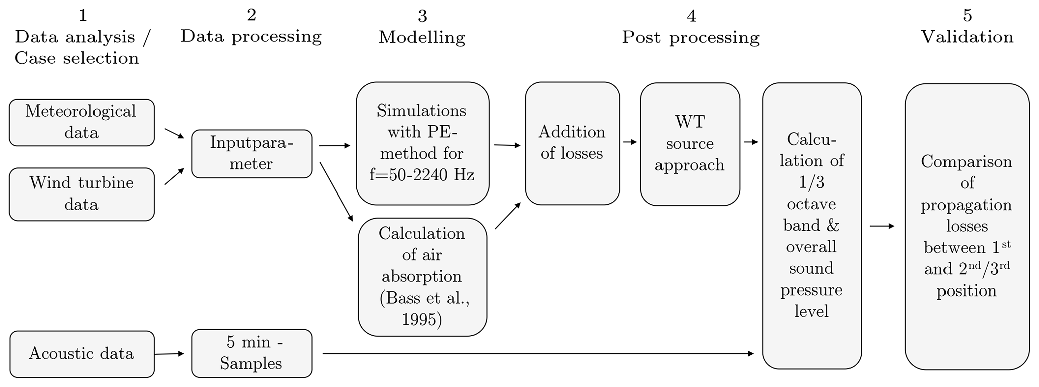
Figure 3 Scheme for validating a sound propagation model with wind turbine noise measurement data.

In the first step, the validation cases are selected based on a data analysis. When selecting the validation cases, it was guaranteed that homogeneous atmospheric conditions were present. For this purpose, the approach described in Argyle and Watson (2014) was adopted. Accordingly, the atmospheric data sets used were compared with data sets recorded within 20 min before and after. The atmosphere was classified as inhomogeneous if in this period of 50 min the wind speed varied by more than 20 %, wind direction by 15^∘ or temperature by 0.5 ^∘C. In addition to that approach, it is assumed that no particular atmospheric phenomena prevailed during the recording of the selected data sets. For example, it was ensured that no low-level jets were present. Thus, the measured wind speed increases steadily with height and no local wind maxima are shown in the vertical profile. This analysis is based on the measurements between altitudes of 27 and 100 m. Hence, low-level jets located above 100 m cannot be noted. Besides homogeneous conditions, it was ensured that the data did not deviate from the power curve of the turbine and that the noise of the wind turbine was dominant.

In the second step of the validation, the measured data are processed. Based on the meteorological and wind turbine data, the input parameters for the sound propagation model are derived. Hub height and rotor length of the wind turbine are considered for the representation of the source. Moreover, the receiver height in the model is set equal to the microphone height during the measurements. Consequently, the same receiver positions relative to the wind turbine are examined in measurements and simulations. In addition to the measurement geometry and the wind-turbine-related parameters, the calculated profile of the effective sound speed, which occurred during the measurement time, is implemented (see Sect. 2.1). Acoustic data samples of 5 min are processed for the comparison of modelled data. In order to guarantee a high level of wind turbine noise, the acoustic data sets were analysed and checked by listening tests (see Sect. 3.1).

In the third step, simulations are performed for one-third octave bands with centre frequencies (f_i) from 80 to 2000 Hz. Higher one-third octave bands have been neglected because of the typical emission spectra of wind turbines and especially because of the atmospheric absorption. Due to measurement inaccuracies caused by wind-induced noise at the microphone, bands lower than 80 Hz are also excluded. Within the one-third octave bands, a sampling rate of Δf=5 Hz is chosen for the simulations, which proved to give sufficient accuracy. The simulations with the PE method are performed for point sound sources at three wind-turbine-related heights, i.e. at hub height h and at ±85 % of the rotor length l. In addition, the air absorption is calculated for the same frequency range.

In the post-processing of the modelled data (step 4), the sound pressure level per frequency is calculated according to Eq. (1). Moreover, the wind turbine source approach is applied to the calculated relative sound pressure level. Between lower and upper limit frequencies of the one-third octave bands, the modelled results at the receiver location m are summed logarithmically:

$$\begin{array}{}\text{(11)}& L_{\mathrm{p},i}\left(f\right)=\mathrm{10}\cdot {\log }_{\mathrm{10}}\left({\mathrm{10}}^{\frac{L_{\mathrm{p},\mathrm{1}}}{\mathrm{10}}}+{\mathrm{10}}^{\frac{L_{\mathrm{p},\mathrm{2}}}{\mathrm{10}}}+\mathrm{\dots }+{\mathrm{10}}^{\frac{L_{\mathrm{p},n}}{\mathrm{10}}}\right),\end{array}$$

where L_p,i(f) is the calculated relative sound pressure level with the band number i. For the same frequency range, the measured data are also processed to one-third octave bands averaged over 5 min with dominant wind turbine noise. Besides one-third octave bands, the overall sound pressure level between 80 and 2000 Hz is determined analogously for measured and modelled data.

In the last step, a comparison of measured and simulated results is performed. Since the sound source cannot be accurately reproduced in either the simulation or the measurements, the first receiver is used as a reference to calculate the propagation loss in both cases. In this way, additional error impacts due to inaccurate representation of the wind turbine can be reduced. The propagation loss is therefore estimated between the first microphone and other microphone positions by

$$\begin{array}{}\text{(12)}& \mathrm{\Delta }{L}_{\mathrm{p}}=L_{\mathrm{p},\mathrm{1}}-L_{\mathrm{p},m},\end{array}$$

where L_p,m is the relative sound pressure level at the receiver position m. Hence, L_p,1 is the relative sound pressure level at the first microphone position.

3 Results

For the comparison of measured and simulated data, different validation cases were derived. In all cases, the wind turbine is characterised by a hub height of 119 m and a rotor diameter of 114 m. The receiver positions are at a height of 1.70 m and at distances of 178, 535 and 845 m from the turbine. The selected validation cases are summarised in Table 3 and are grouped in terms of the propagation direction. They are grouped into light downwind (case 1, 2), crosswind–downwind (case 3, 4), crosswind–upwind (case 5, 6), light upwind (case 7, 8) and strong upwind (case 9, 10). In the figures of the paper, the different groups are colour-coded in red (downwind, case 1) through orange and green to blue (upwind, case 10). Each group contains two validation cases that have very similar propagation characteristics. The data acquisition within a group took place in the same night and within 2 h.

Table 3 Overview of validation cases.

In this section the different validation cases are first analysed in terms of environmental conditions and acoustic properties. Subsequently, the validation is performed by comparing measured and modelled propagation losses per one-third octave band and overall sound pressure levels. Afterwards, the validation results are discussed regarding model assumptions and the effect of input parameters.

3.1 Analysis of measured data

3.1.1 Environmental conditions

Since wind direction and wind speed are key determinants of the sound speed profile, these parameters are particularly important for sound propagation and are described using Fig. 4. The wind speed and direction measured respectively at 100 and 95 m at the time of validation cases are shown in Fig. 4a. In Fig. 4b, the calculated profiles and the measured values of the effective sound speed are also given. The different groups of propagation direction are clearly seen. The cases of each group provide similar characteristics regarding wind direction, wind speed and effective sound speed profile. Since the data were recorded within the same 30 min, the cases in the strong upwind direction show almost the same effective sound speed profile.

The accuracy of the calculated sound speed profiles is assessed by the root mean square error (RMSE). This value indicates the average deviation of the profile from the measured values. The RMSE values were calculated for the fitting of sound speeds over all cases. The averaged RMSE value of all cases is 0.04 m s⁻¹ so that in general a very good fitting of the sound speed profile is concluded. This assessment is based on a comparison with literature values, where values of about 0.15 m s⁻¹ are described as sufficiently accurate (Heimann and Salomons, 2004). The worst fit is seen for case 9 with an RMSE of 0.14 m s⁻¹. The best fit is achieved for case 4 with RMSE = 0.0017 m s⁻¹.

Figure 4 (a) Distribution of measured wind speed and wind direction at 100 and 95 m height respectively. (b) Derived profiles of effective sound speed (lines) based on measured data at four heights (markers), normalised with the effective sound speed at 1 m. The wind directions are related to the microphone positions so that a direction of 0^∘ indicates upwind conditions, whereas a direction of 180^∘ represents downwind conditions. For both graphs the legend on the right side is used.

The profile of the effective sound speed generally displays the different atmospheric stabilities. However, a better measure for the stability is the wind shear exponent, which, calculated according to Eq. (10), is listed for all cases in Table 4. With an exponent of over 0.6, cases are assigned to a very stable atmosphere, while the values between 0.2 and 0.4 belong to a slightly stable atmosphere. The cases of each group have very similar values for the exponent. In general, no validation cases are presented for neutral and unstable atmospheres, which would show wind shear exponents below 0.2. This is related to the fact that measuring at unstable situations provides lower signal-to-noise ratios. Stable atmospheres are predominantly developed at night, where extraneous and ambient noise is low compared to daytime activities. Moreover, in comparison to an unstable atmosphere, the wind speed on the ground is low, which reduces the wind-induced noise. This refers to wind-induced noise at the microphone and to natural wind-induced noises such as leaf rustling. Consequently, the signal-to-noise ratio is greater with stable stratification, and thus the quality of the measurement data is higher than with unstable or neutral stratification. The atmospheric values of temperature and relative humidity significantly determine the air absorption, whereas they have a subordinate effect on the sound speed profiles. The averaged values as well as the standard deviation over 10 min are visualised for temperature and relative humidity in Fig. 5a. As before, the pairs have similar values. With about 1 ^∘C difference, cases 5 and 6 have the largest temperature discrepancy. Humidity differs the most between cases 1 and 2, amounting to 10 %. In both cases, the high standard deviations of the humidity values of up to 45 % are remarkable. A high standard deviation of the humidity might indicate frequent rainfall so that in these cases explicit attention must be paid to the quality of the measurement data. Lastly, the calculated values of the atmospheric air coefficient α_L (dB km⁻¹) for the mid-frequencies of the one-third octave bands are visualised in Fig. 5b for three selected cases. As expected, the coefficient and thus the sound absorption increase with increasing frequency and decrease with increasing temperature and humidity. Case 3 is characterised by low values of humidity and temperature and has a sound absorption of 13 dB km⁻¹ at 2000 Hz. As a result of higher humidity and temperature, case 10 has a lower sound absorption of 9 dB km⁻¹ at the same frequency.

Table 4 Calculated wind shear exponent at the time of the validation cases.

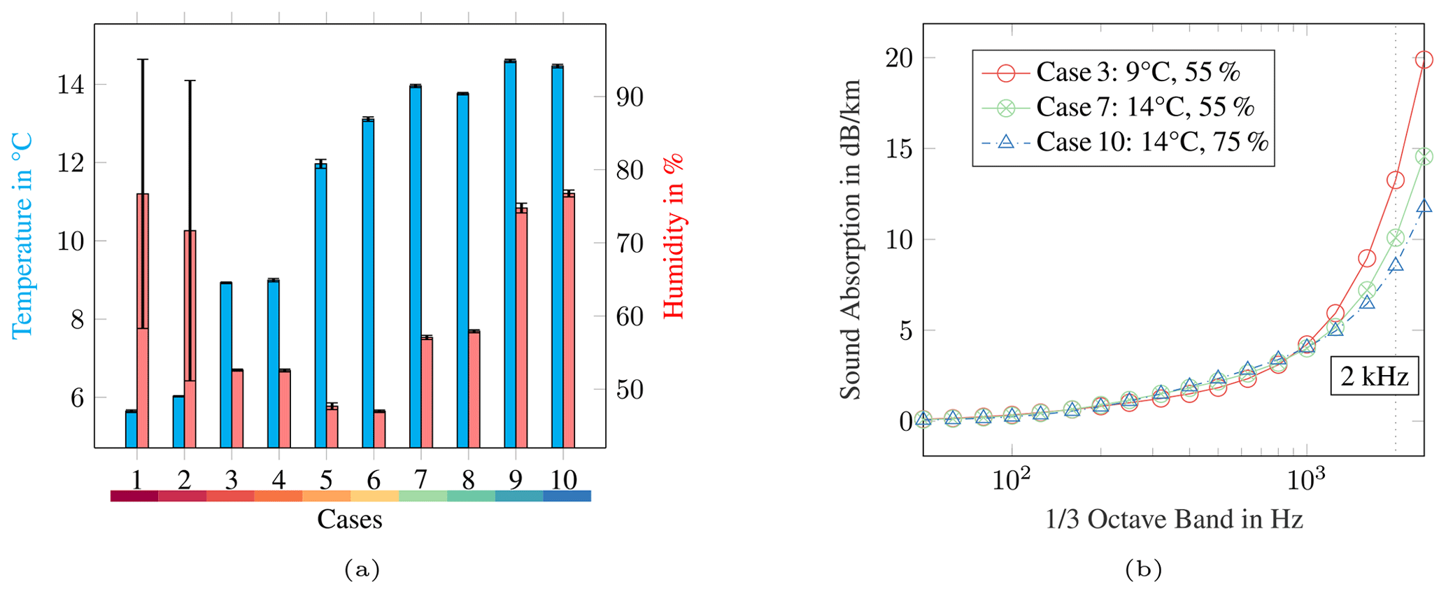
Figure 5 Parameters describing the atmospheric air absorption for the validation cases. (a) Measured values and standard deviation of 10 min data for temperature and relative humidity at 53 m. (b) Calculated sound absorption for selected cases having similar values of temperature and relative humidity.

3.1.2 Acoustic data

The signal-to-noise ratio (SNR) is of particular importance for the quality of the acoustic data. It represents the difference between the desired sound and background noise, i.e. in the present case the difference between the noise of the wind turbine and extraneous noise. In general, the latter includes all types of background noise, such as noise from traffic or animals, which have a significant influence on the measurements. In order to select validation cases without these significant extraneous noises, frequency-dependent selections and listening tests were performed. Frequency-dependent selection is a common methodology in which the frequency spectrum of the wind turbine is compared with spectra including extraneous noise (van den Berg, 2004; Larsson and Öhlund, 2014; Conrady et al., 2018; Martens et al., 2020).

In order to assess the background noise, recordings were conducted at the beginning of the measurement campaign during wind turbine shutdown. Here, the background noise was measured with the same measurement setup at comparable wind conditions. The measured background noise is considered to be representative of the background noise that occurred during the measurement of the validation cases. It should be mentioned that the wind turbine operations (on/off) were regulated by the power production management system. This means that the authors did not control the operational conditions of the wind turbines – neither for the turbine under investigation nor for the surrounding turbines (see Fig. 1). In times of high energy production within the whole energy system, however, the management system deliberately shuts down turbines so that recordings of background noise are possible even at operating wind speeds. Following the measurements of background noise, the authors benefited from the fact that the wind farm is also a test site. Even if surrounding turbines were switched off by the management system, the turbine under investigation continued to operate in test mode. As a result, measurements for the individual turbine were possible.

In Fig. 6 the measured background noise per one-third octave band is shown for different wind speeds at the three microphone positions.

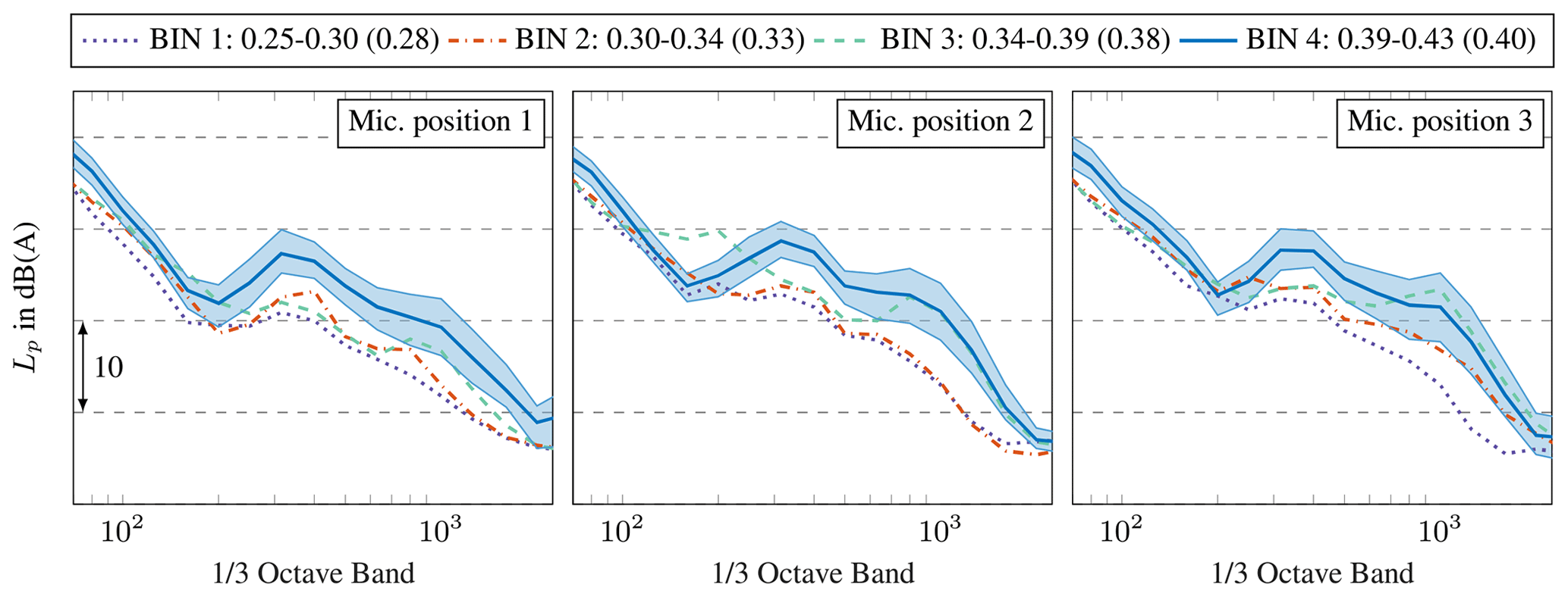
Figure 6 Measured background noise per one-third octave band for different wind speed bins at three microphone positions. The wind speeds were recorded at a height of 100 m and are divided into bins of 1 m s⁻¹. The bins are normalised to the cut-off wind speed of the turbine. The average normalised wind speed during the background noise measurements is given in parentheses. The measured sound levels in the bins are energetic averages over the corresponding measurement period. Representative of all bins, the standard deviation of the measurements is given for bin 4, which includes the data at the highest wind speed during the background measurements.

A similar tendency is noticeable at all microphones. With increasing wind speed, the background noise increases. This trend is already known from the literature and is due to the wind-induced noises that depend on the wind speeds. High extraneous noise in the low-frequency range is due to wind-induced noise at the microphone, which cannot be completely eliminated even with effective windscreens. In Fig. 6, a local peak at approximately 300 Hz is also observed. This is assumed to be wind-induced vegetation noise, such as the rustling of grasses. The peak at 1000 Hz is due to a combination of vegetation noise and the A-weighting of the sound level. In general, the standard deviation of the background measurements is higher than for the wind turbine noise. As seen in Fig. 6, the highest value is at the local level maxima with approximately 2.5 dB. Wind-induced sounds from vegetation are known to vary greatly. Consequently, it is assumed that this variation is responsible for the comparatively high standard deviations. Since the recordings were conducted before the measurement campaign, it should be noted that the background noise can change in the course of the measurement campaign depending on the vegetation. Due to prevailing wind conditions and the management system, no measurements of background noise could be taken at the end of the measurement campaign.

After all, in Fig. 7 the calculated SNR is shown per one-third octave band at the three microphones for five selected cases, i.e. one case per group. To consider the most critical condition, the background noise at bin 4 is used for the determination of SNR. In the guideline IEC 61400-12 (2012), three quality levels are stated. An SNR of more than 8 dB is very good and between 3 and 8 dB is sufficient. If the difference is less than 3 dB, it is recommended not to use the measurements.

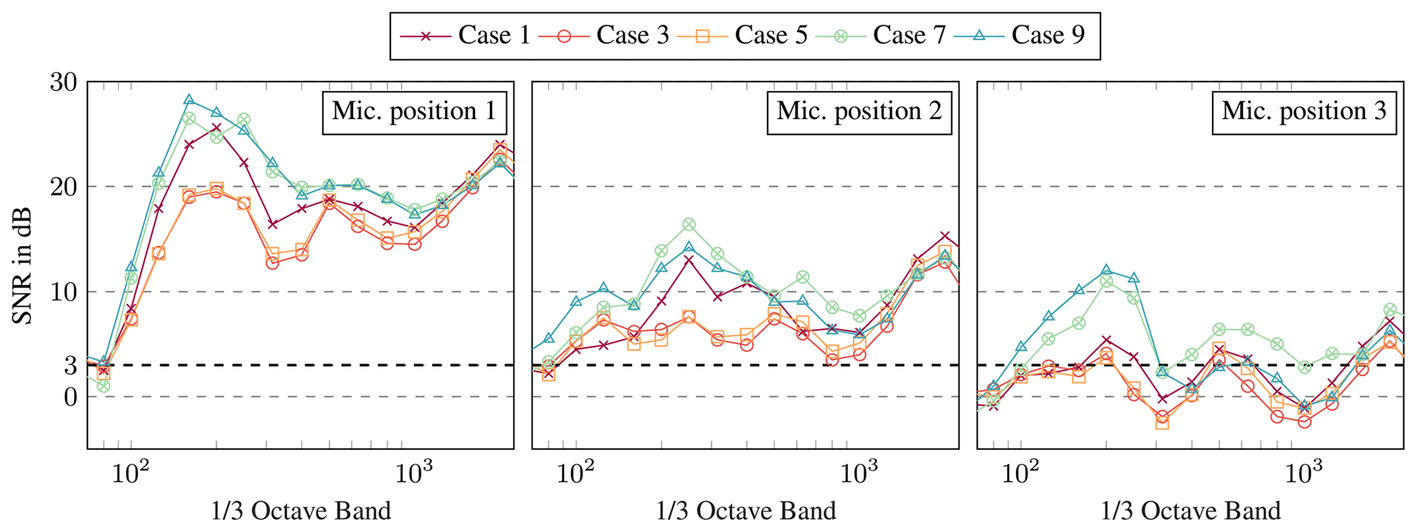
Figure 7 Signal-to-noise ratio per one-third octave band for selected cases at three microphone positions. The background noise at bin 4 is used for the determination.

In general, the SNR decreases with increasing distance, which is due to the quieter wind turbine noise. While a sufficient SNR is usually achieved at Mic 1 and Mic 2, the SNR at the third microphone is critical. Here the values for crosswind conditions, in particular, are below 3 dB and are partly in the negative range. Moreover, Mic 1 indicates that very low frequencies below 100 Hz, in particular, are also classified as critical. Wind-induced noise at the microphone is considered in these low-frequency ranges. In addition, compared to other cases, a low SNR is calculated with the cases in crosswind conditions at the first microphone position. This tendency is also observed at positions two and three. The comparatively low SNR in the crosswind condition is due to the source characteristics of the turbine. Because of the dipole characteristic of the trailing edge noise, a wind turbine radiates less sound in the crosswind direction. Consequently, the difference to the background noise is lower in this direction.

Especially at Mic 3 at a distance of 845 m from the wind turbine, the SNR is critical. However, to extend the database those data are also used for the validation. By carefully listening to the recordings of the validation cases, a negligible influence of the background noise on the useful signal is ensured. It should be stated that the highest wind speed bin (bin 4) was chosen in the analysis of SNR – even though some of the validation cases were recorded at lower wind speeds. That means the worst scenario was investigated. In addition, only two measurements over a period of 5 min were available for bin 4. It can be expected that the wind turbine noise is dominant at the third microphone for all cases.

3.2 Validation

The measurement data are used to validate the sound propagation model presented in Sect. 2.1. The measured and modelled sound propagation losses between the first and the second as well as between the first and the third microphone position are compared using one-third octave bands and overall sound pressure levels. For assessing the accuracy and for quantifying the validity of the model prediction, the mean difference between measured and modelled propagation loss over frequencies is introduced. The modelled propagation losses include all attenuation terms introduced in Sect. 2.1, i.e. attenuation due to geometric scattering, air absorption and other aspects such as ground effects and atmospheric refraction.

3.2.1 Comparison of one-third octave band

The comparison of measured and modelled sound propagation losses per one-third octave band is shown using Fig. 8. For a better overview, the standard deviations of the measured data are only given for one case of each group. In addition to the sound propagation losses, the corresponding profiles of effective sound speed are given. Since cases 5 and 6 show similar results to cases 3 and 4 and provide no new findings, their results are given in the Appendix. In the following, the differences within the groups are presented first. Subsequently, cases 1 to 10 (Fig. 8) are discussed in detail.

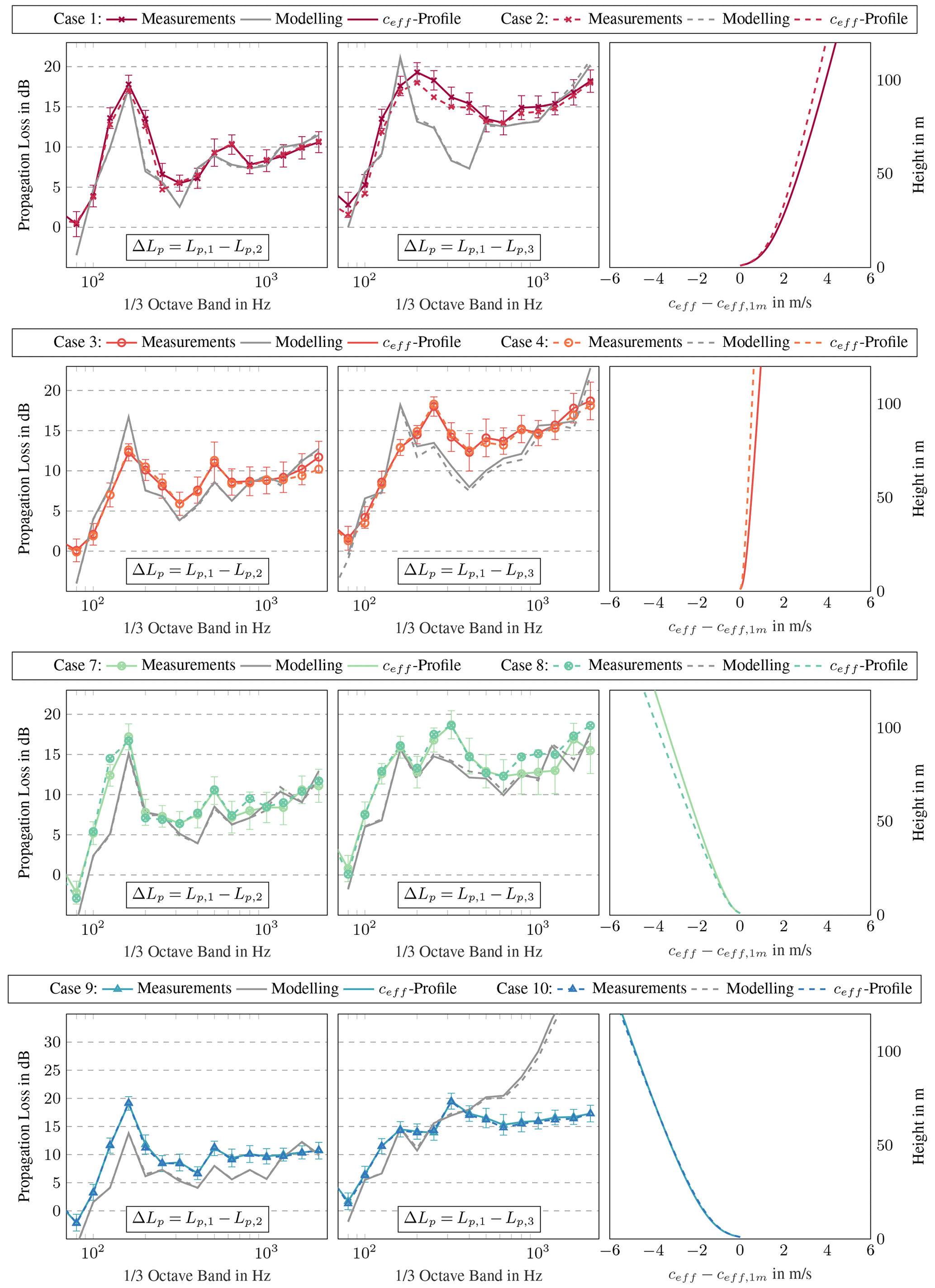
Figure 8 Comparison of measured and modelled sound propagation losses per one-third octave band for cases 1 to 4 and 7 to 10. Left: propagation losses between Mic 1 (178 m) and Mic 2 (535 m) including standard deviation for one measurement case. Middle: propagation losses between Mic 1 (178 m) and Mic 3 (845 m) including standard deviation for one measurement case. Right: normalised profiles of effective sound speed.

In general, the difference within the groups is very small. In groups of similar propagation conditions, very similar sound propagation losses are measured or modelled. For example, the averaged difference in the measured values of cases 1 and 2 (group 1) is only 0.28 dB between Mic 1 and Mic 2. The averaged difference of the modelled data is 0.24 dB. Consequently, it is assumed that the accuracy within the measurements and the modelling is sufficient.

For cases 1 to 8, the measured and modelled sound propagation losses between the first and second microphone positions agree well. In all cases, the propagation losses are at similar levels. Moreover, the peak of the losses is reproduced in the modelling. In both the measurements and the modelling, maximum sound propagation losses are obtained at frequencies of 160 and 630 Hz. This is due to ground reflections and the subsequent interference. In all cases, the measured and modelled losses increase significantly with higher frequency at greater distances, e.g. between the first and third microphone. This is caused by the frequency-dependent air absorption.

With higher distances, i.e. for losses between 178 and 845 m, a more pronounced discrepancy between measured and modelled values is observed. Here, the curve characteristics between 160 and 400 Hz differ. Those differences are further addressed in the following.

In the downwind direction (cases 1 and 2), the measured peak is observed over a broader frequency spectrum when compared to the modelled spectrum. At the band with a centre frequency of 400 Hz, the difference between measured and modelled values is approximately 7 dB. This difference could be due to changed ground properties. Due to the large standard deviation of humidity (see Sect. 3.1), an increased probability of rainfall is present during the period of cases 1 and 2. The propagation attributes and correspondingly the losses change with wet grass. The influence of different ground conditions on sound propagation is shown in Sect. 4.2.

For crosswind conditions (cases 3 and 4), for the measured losses between 178 and 845 m, the peak is shifted to 250 Hz, which corresponds to a shift of two bands. In the modelling, the peak is still very pronounced at 160 Hz, although a local maximum is identified at 250 Hz. However, this is much less pronounced than in the measurements.

For upwind conditions (cases 7 and 8), two peaks at 160 and 250/315 Hz are evident in the measured and modelled losses for larger distances. With increasing distance, the refraction effects, which depend in particular on the effective sound speed profile, become more important. The sound is refracted upward in upwind conditions, while it is refracted downward in downwind conditions. Accordingly, especially at long distances, the incidence angles to the ground and thus the frequency-dependent ground reflections change in terms of the sound speed profile. As a result, the curve characteristics change depending on sound speed profiles and, hence, sound direction.

Cases 9 and 10 are characterised by strong upwind conditions. In Fig. 8, modelled results are presented without turbulence. The effect of turbulence is clearly seen in the modelled sound propagation losses between 178 and 850 m. Due to the upward refraction, a shadow zone is created in strong upwind conditions. Since sound waves cannot enter the shadow zone directly, the propagation losses modelled without turbulence increase significantly at high-frequency ranges. The propagation losses reach up to 50 dB. In reality, the sound waves are scattered at turbulent eddies and consequently enter the shadow zone. Hence, these strong losses are not present in the measurements. However, the measured sound pressure levels also become lower in the shadow zone. In addition, the background noise in the high-frequency range is critical so that the identification of the wind turbine noise is difficult above 1000 Hz. While the model overestimates the sound levels at a greater distance, an underestimation is observed at a smaller distance. Here, the modelled losses are about 4 dB lower than the measured ones.

3.2.2 Comparison of overall sound pressure level

The overall sound pressure levels are calculated considering the examined frequency bands (80 to 2000 Hz). The differences between measured and modelled propagation losses in overall sound pressure levels between 178 and 535 and between 178 and 845 m are shown in Fig. 9. A negative value implies an overestimated and a positive value an underestimated prediction of the propagation losses. For directions other than strong upwind, the model generally predicts the propagation losses in overall sound pressure level well. The differences between model and measurements are less than 2 dB. Due to the neglect of turbulence scattering in the simulations, the differences in the strong upwind direction exceed 20 dB at 845 m. Because of shadow zones, turbulence effects become more important with increasing distance.

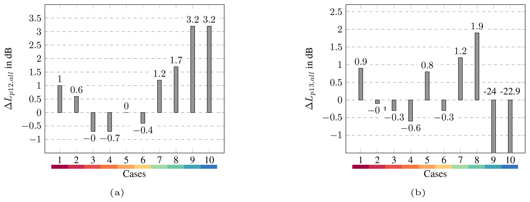
Figure 9 Difference of measured and modelled overall propagation losses between (a) Mic 1 (178 m) and Mic 2 (535 m) and between (b) Mic 1 (178 m) and Mic 3 (845 m).

3.3 Validity of model prediction

To evaluate the validity of the model prediction in one-third octave bands, the mean of the absolute difference between measured and modelled propagation losses is calculated over the frequency band i:

$$\begin{array}{}\text{(13)}& \mathrm{\Delta }{L}_{\mathrm{p},\mathrm{mean}}={\displaystyle \frac{\mathrm{1}}{N}}\sum _i^N\left|\mathrm{\Delta }{L}_{\mathrm{p},\mathrm{modell}}\left(f_i\right)-\mathrm{\Delta }{L}_{\mathrm{p},\mathrm{meas}.}\left(f_i\right)\right|.\end{array}$$

Calculated ΔL_p,mean is shown in Fig. 10. Between 178 and 535 m, ΔL_p,mean is between 1.6 dB (case 2) and 3.2 dB (case 9). For all cases, ΔL_p12,mean increases with greater distance. ΔL_p13,mean is between 2.2 and 8.3 dB. Since turbulence is not taken into account in the simulations, the measured and modelled one-third octave spectra differ the most in the strong upwind direction. For the other wind directions, ΔL_p13,mean smaller then 3.2 dB is obtained. The difference for case 1 (3.2 dB) is due to the broad measured peak in the middle-frequency range (see Fig. 8).

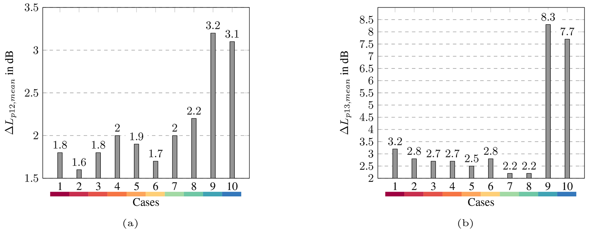
Figure 10 Difference of measured and modelled overall propagation losses between (a) Mic 1 (178 m) and Mic 2 (535 m) and between (b) Mic 1 (178 m) and Mic 3 (845 m).

4 Discussion

Discrepancies between measured and modelled one-third octave spectra are observed, especially at greater distances. To discuss these discrepancies, the modelling of the sound source and the ground effects will be addressed in the following. In addition, the homogeneity of the atmospheric parameters and the influence of time-averaging the measured data are addressed. Accordingly, the discussion in this paper focuses on the essentials. General limitations of the PE method, which are described in detail in Salomons (2001), are not presented.

4.1 Source modelling

The chosen method representing a wind turbine as a sound source is simplified. As in Nyborg et al. (2022), three incoherent sound sources with equal source strength are assumed. This simplification is necessary due to insufficient information about the individual point sources and the source distribution over height. Verification of the validity of these assumptions is beyond the scope of this work. However, many prediction models and guidelines assume that the sound source of a wind turbine is a monopole source located at the hub height of the turbine (e.g. ISO 9613-2, 1996; Lee et al., 2016). Ecotière (2015) shows that this assumption is not suitable for spectral analysis, as effects of ground reflections are not well represented using one point source. Nyborg et al. (2022) determine that the agreement with measured spectra was significantly improved with three distributed point sources. With increasing distance, the difference between the results of one source and three sources decreases.

Figure 11 Schematic illustration of the setup with 1, 3 and 10 point sources.

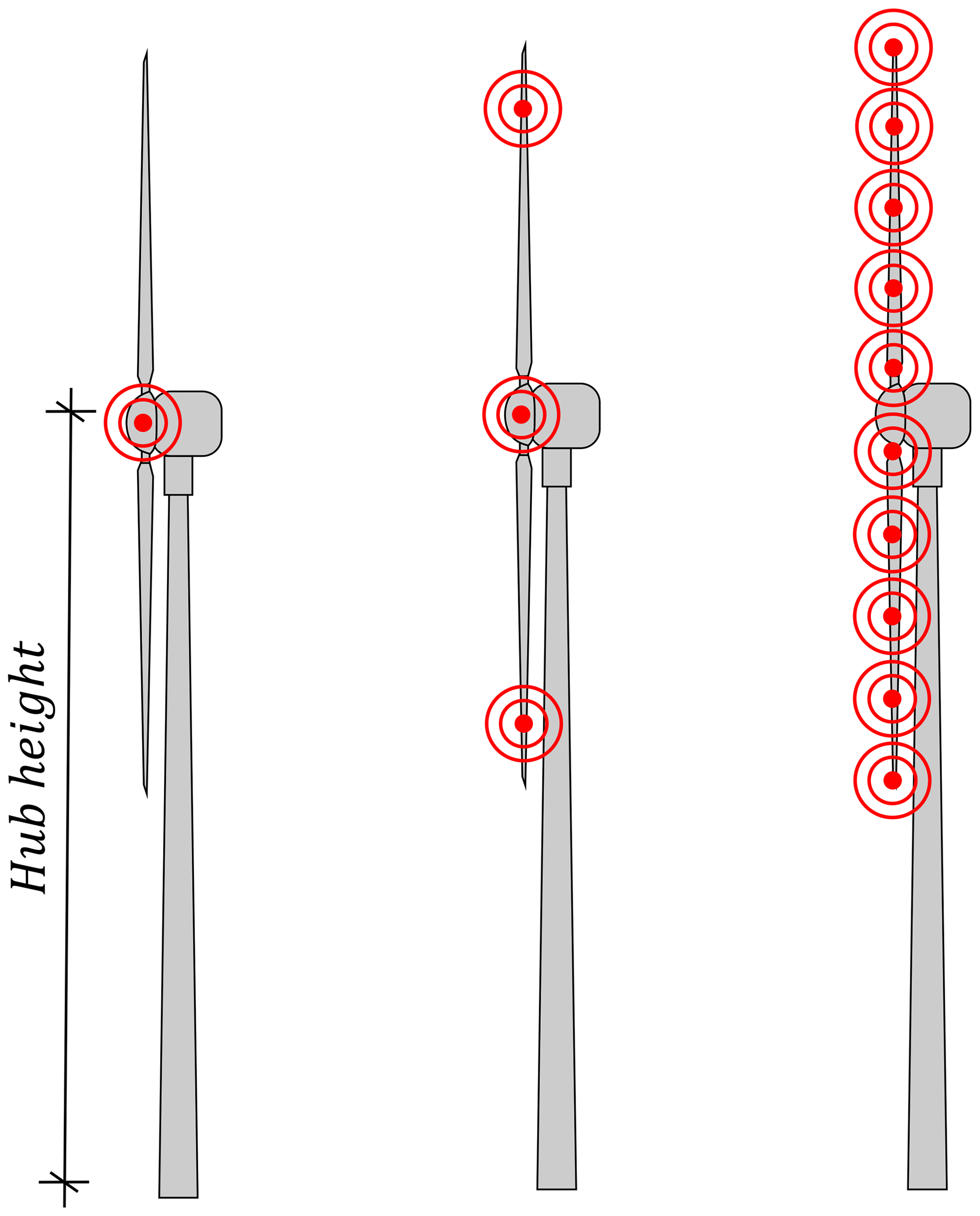
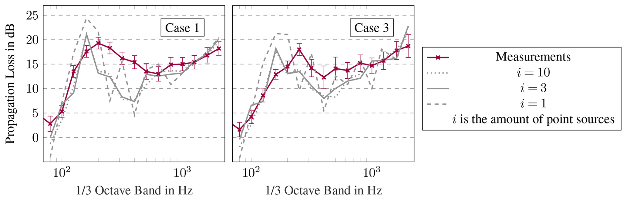
Figure 12 Comparison of measured and modelled sound propagation losses between 178 and 845 m with different numbers of sound sources i per one-third octave band.

To investigate the influence on the sound spectrum, simulations with 1, 3 and 10 point sources are compared. In the latter case, 10 point sources are distributed over the rotor diameter. In Fig. 11, the setup of 1, 3 and 10 point sources is illustrated schematically. The results of the first and the third validation cases between 178 and 845 m are shown in Fig. 12. Several peaks and valleys are observed in the one-third octave spectrum with one point source. They are due to interference effects and are smoothed in reality by superimposing the interference patterns of multiple sources. This is also shown in Heutschi et al. (2014), Cotté (2019) and Nyborg et al. (2022). Compared to multiple sources, the monopole model results reproduce the one-third octave spectrum of the sound propagation losses less well and deviate more from the measurements. The results with 3 and 10 monopole sources are very similar to each other.

Simply increasing the number of sources beyond three does not improve the accuracy. The possibility that the discrepancies in the one-third octave spectrum are at least partly due to the assumptions in the source modelling cannot be excluded.

4.2 Ground properties

For various reasons, such as a changes in soil humidity, the ground property can vary between cases. Since the cases with the same wind direction are close in time (see Table 3) and have similar measured spectra (see Fig. 8), it is assumed that they have similar soil conditions. However, the soil conditions can vary between cases with different wind directions, which can have a significant impact on the one-third octave spectra and may explain the discrepancies between modelled and measured data at 845 m. In addition, the soil conditions can change along the propagation path. As the model used assumes constant ground conditions along the propagation path, this cannot be investigated in this paper.

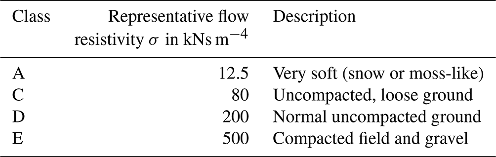
In the Delany–Bazley model, the ground impedances are only related to the flow resistivity. Hence, the influence of ground properties on the one-third octave band is examined by selected representative values of flow resistivity, which are based on the classification given in Plovsing and Kragh (2000). The classification including the values of flow resistivity and a description are summarised in Table 5. Accordingly, values from 12.5 kNs m⁻⁴ (very soft) to 500 kNs m⁻⁴ (compacted field) are considered and discussed. As before, this discussion is representatively performed on the example of the first and the third validation case and for the larger distance of 845 m. The measured and simulated losses at different ground impedances are plotted per one-third octave band in Fig. 13.

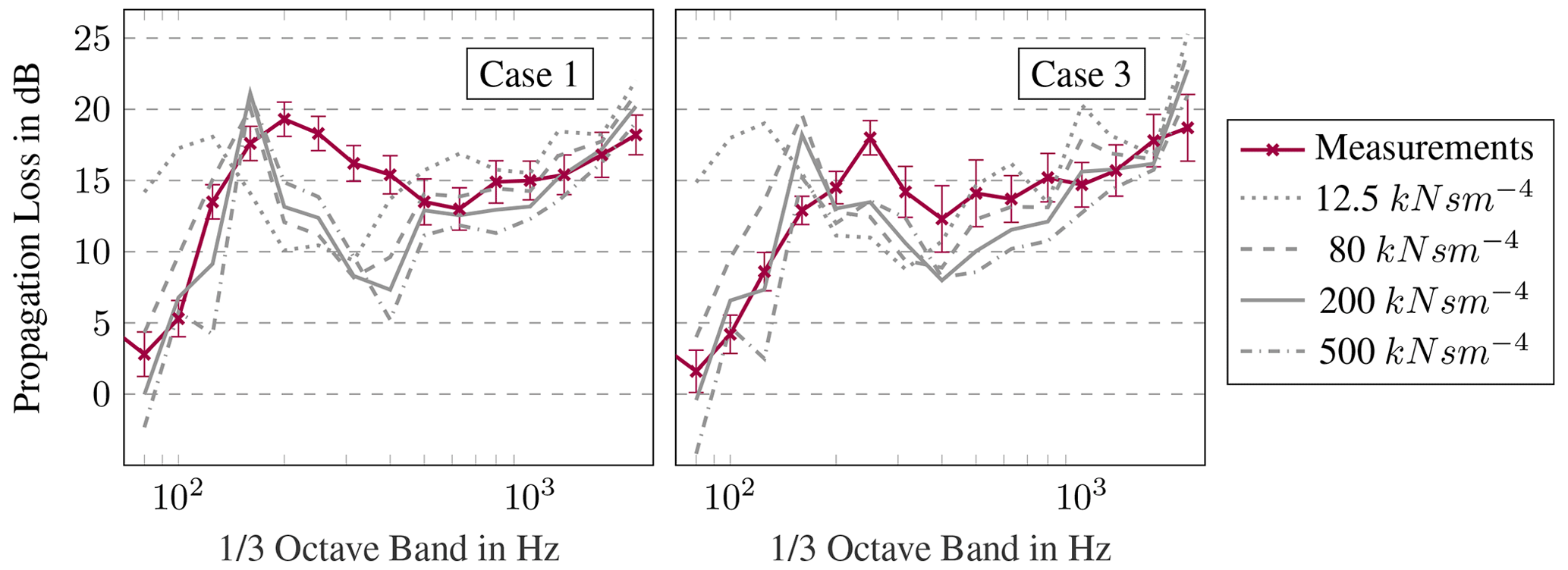
Figure 13 Comparison of measured and modelled sound propagation losses between 178 and 845 m, with representative values of flow resistivity per one-third octave band.

Table 5 Classification of selected ground impedance types, i.e. values of flow resistivity according to Plovsing and Kragh (2000).

For both cases, the selected ground impedances have an impact on the level of propagation losses as well as on the position and width of the propagation peak. Generally, lower flow resistivity results in higher propagation losses. This is due to the increased absorption and/or decreased reflections at the ground for lower values of flow resistivity. Consequently, higher propagation losses are modelled with moss-covered ground (12.5 kNs m⁻⁴) than with compacted fields (500 kNs m⁻⁴). In addition, a broader propagation peak with decreasing values is observed in Fig. 13. This phenomenon is not caused by the increasing absorption but by a phase shift between the incident and the reflected wave. At very low values, like 12.5 kNs m⁻⁴, the peak is broader and also shifted towards lower frequencies. Evidently, the soil conditions have a significant impact on the sound propagation loss. Simply changing the flow resistance does not clarify the cause of the discrepancies in one-third octave spectra and does not lead to better validation results.

4.3 Homogeneity of atmospheric parameters

In general, the atmospheric parameters are affected by the topography of the wind farm. As described in Sect. 2.2, the terrain of the wind farm is flat. The area consists mainly of meadows, agricultural land and single ditches. Isolated trees with a height of 10 to 20 m and buildings are only present at the edge of the wind farm at a distance of about 1 km. Therefore, the influence of the topography on the measured data is considered insignificant.

To analyse the homogeneity of the atmospheric parameters, the wind turbine SCADA data are compared with the data from the 100 m mast. The 100 m mast is located approximately 2 km north-west of the wind turbine. It should be noted that the turbine operation can affect the meteorological measurements at the hub height. The comparison between the data is shown in Fig. 14. Measured values of temperature and wind direction as well as profiles of wind speed and normalised effective sound speed are presented.

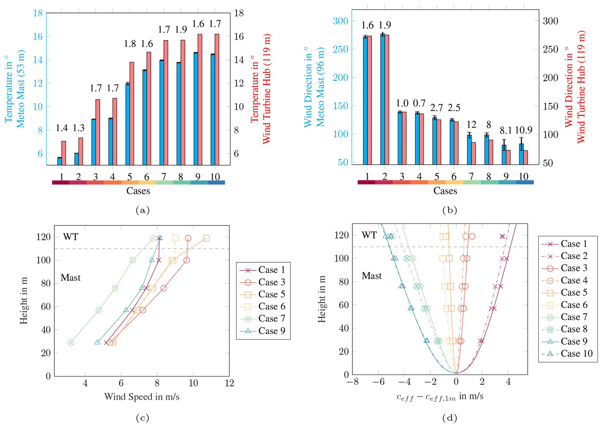
Figure 14 Comparison of atmospheric data measured at the 100 m mast and at the wind turbine (119 m). (a) Temperature measured at 53 m on the meteorological mast and at the wind turbine hub (119 m). (b) Wind direction measured at 96 m on the meteorological mast and at the wind turbine hub (119 m). In panels (a) and (b), the differences between the data are written above the bar, and the standard deviations are given for the mast measurements. (c) Wind speed measured at various heights on the meteorological mast and at the wind turbine hub (119 m). (d) Profiles of effective sound speed (lines) based on measured data (markers), normalised with the effective sound speed at 1 m.

In Fig. 14a, the measured temperatures at the meteorological mast (53 m) and at the wind turbine (119 m) are compared. As the temperature measurements at the mast height of 95 m are erroneous, a direct comparison is not possible. In all validation cases, the temperature measured at the hub height of the turbine is 1–2 ^∘C higher than the temperature measured at 53 m height on the meteorological mast. Accordingly, the temperature increases with height, indicating a stable atmosphere and an inversion situation.

Figure 14b shows the measured wind directions at a height of 95 m (meteorological mast) and 119 m (wind turbine). With differences of more than 8^∘ and relatively high standard deviations, the measured data particularly differ in the upwind direction (cases 7 to 10). Herein, case 7 (12^∘) and case 10 (11^∘) are prominent. Similar wind directions were measured for the other cases. The differences are less than 3^∘.

In Fig. 14c, the measured wind speeds at the mast (29, 57, 76, 100 m) and at the hub height of the wind turbine (119 m) are plotted against height for the selected cases. In most cases, slightly higher wind speeds are measured at 119 m than at 100 m. For case 5, for example, the wind speed increases by about 2 m s⁻¹ from 100 to 119 m. For case 1, the wind speed at 119 m is slightly lower than at 100 m.

For sound propagation, the profiles of the effective sound speed are essential. The calculated profiles and the values of the effective sound speed determined with the measured data are shown in Fig. 14d. While the temperature has a negligible effect on the effective sound speed, the differences in measured wind direction and wind speed are reflected in the effective sound speed. Due to the large differences in the measured wind directions, the calculated values at 119 m deviate from the profile in case 7. The deviation is approximately 1 m s⁻¹. Similar deviations can be seen for case 1. These deviations are due to the difference in wind speed. For cases 1, 7 and 8, the profile of the effective sound speed could be changed slightly when the SCADA data were included. This is expected to have a negligible impact on the validation results.

4.4 Effect of time-averaging the measured data

As short-term fluctuations of the meteorological parameters can affect the measured acoustic data, the influence of averaging meteorological and acoustic quantities on the validation results is examined. The first case is taken as an example, and four averaging time periods are considered: 1, 3, 5 and 10 min.

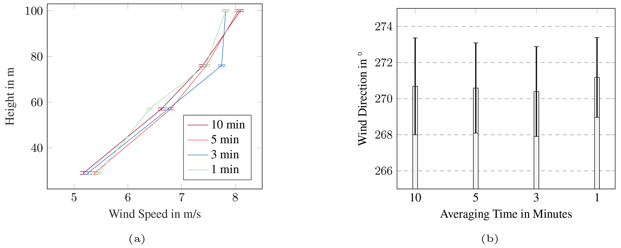
Figure 15 Measured wind speed and wind direction averaged over 10, 5, 3 and 1 min and its standard deviation. (a) Measured wind speeds at different heights on the meteorological mast. (b) Measured wind direction at 96 m on the meteorological mast.

In Fig. 15a and Fig. 15b the height-dependent averaged wind speeds and the measured wind directions at 96 m are shown for the analysis periods respectively. The standard deviations are also included and additionally listed in Table 6. For averaging periods of 3, 5 and 10 min, similar wind profiles and wind direction values are observed. When averaging over 1 min, deviations occur in the wind profile. Due to fluctuations, the wind profile does not show the usual logarithmic curve. These short-term fluctuations disappear when averaging over a longer period of time. The standard deviation of the height-dependent wind speed is between 0.33 and 0.59 m s⁻¹. Except for the 1 min averaging, the standard deviation of the wind speed decreases with increasing height and decreasing averaging period. The standard deviation of the wind direction for all periods is similar and is approximately 2.5^∘. Thus, in this case, the wind direction does not depend significantly on the averaging period.

Table 6 Standard deviations of measured wind speed and wind direction for averaging periods of 1, 3, 5 and 10 min.

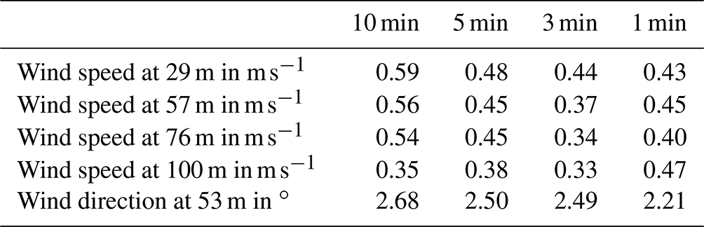
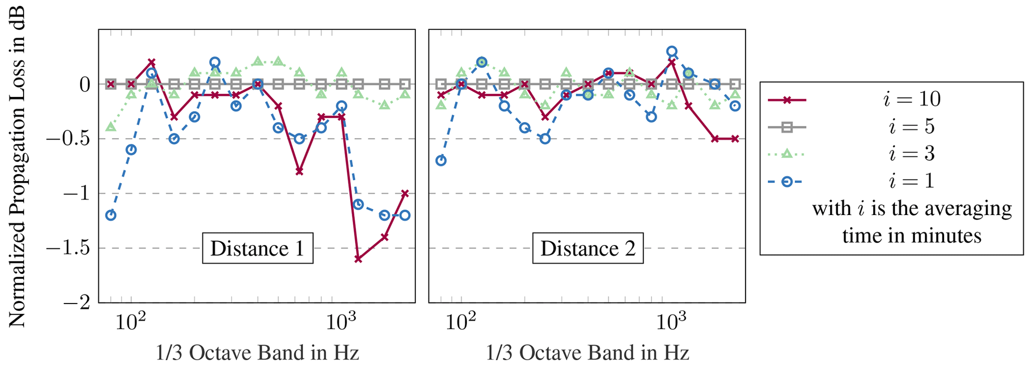
Figure 16 Comparison of measured sound propagation losses between 178 and 535 m and between 178 and 845 m for the different averaging times i per one-third octave band. The data are normalised to the results averaged over 5 min.

Dependent on the four averaging periods, the calculated sound propagation losses between 178 and 535 m and between 178 and 845 m are shown in Fig. 16. Thereby, the losses are related to the propagation losses obtained with an averaging period of 5 min. The measured losses with an averaging period of 3 and 5 min are at a similar level and differ only between −0.4 and 0.2 dB. Losses averaged over 1 and 10 min show more deviations. The maximum deviations are observed in the lower and upper frequency bands. For the sound propagation losses between 178 and 535 m, the maximum difference is 1.6 dB. Between 178 and 845 m, the maximum deviation is smaller (−0.7 dB). Hence, for a few frequencies, the averaging period has an influence on the validation results.

Based on the findings presented, an averaging period of 3 to 5 min is recommended when using the data for validation purposes. This period is long enough to neglect the short-term fluctuations in the meteorological variables, which may differ along the propagation path and cannot be described by the model used in this work. An averaging period of 10 min is not recommended due to the acoustic evaluation. Here, a dominant noise of the wind turbine has to be guaranteed.

5 Conclusion and outlook

The objectives of this paper were to introduce, to prepare, to apply and to provide comprehensive wind turbine noise measurement data for the systematic validation of sound propagation models. Extensive measurement campaigns were carried out in the area of wind turbines, which involved the acquisition of meteorological, acoustic and turbine-specific data. Meteorological quantities, such as wind speed, temperature and humidity, were collected at different heights on a 100 m measurement mast. For the recording of acoustic data, autarkic acoustic measuring stations were positioned at 178, 535 and 845 m from the wind turbine.

The atmospheric and the acoustic quantities were processed and analysed. On this basis, a total of 10 validation cases were identified, which were divided into five groups depending on the direction of sound propagation. Based on the meteorological measurements as well as the SCADA data of the turbine, relevant input parameters for the sound propagation model were derived. In addition to the measurement geometry and information on the determination of air absorption, these also include sound speed profiles.

In this paper, the processed measurement data are used to validate a sound propagation model that applied the Crank–Nicolson parabolic equation method. The validation was performed by comparing the measured and modelled sound propagation losses per one-third octave spectrum and overall sound pressure levels between 178, 535 and 845 m. In general, the agreement between measured and modelled data is not satisfactory in strong upwind conditions, where turbulence is not considered in the model. In the other wind directions, the measured spectrum is well reproduced. In both measurements and modelling, losses increase with increasing frequency due to air absorption. Because of interferences, peaks and valleys of the sound propagation losses exist in the frequency band and are identified in the measured and modelled data. At greater distances, for some cases broader peaks and/or a shift of peaks towards higher frequencies are measured. This is not reproduced by the model, which could be explained by inadequate source and ground modelling. However, the exact cause of these discrepancies could not be identified within the scope of this paper and is, thus, part of future investigations. The comparison between the measured and modelled sound propagation losses in the overall sound pressure level shows good agreement, with the exception of the strong upwind situation.

To assess the validity of the model prediction, the mean of the absolute difference between modelled and measured losses is introduced. For directions other than strong upwind, the mean of the absolute difference is between 1.6 and 3.2 dB.

This paper provides the first step towards the publication of measurement and simulation data in the field of wind turbine sound propagation. The data sets used for the validation are provided as openly accessible for further research purposes. Further data sets will be added in future work. A comprehensive structured data repository will be created, containing anonymised research data on wind turbine sound emission under various atmospheric and operational conditions.

Appendix A: Validation results – comparison of one-third octave band for cases 5 and 6

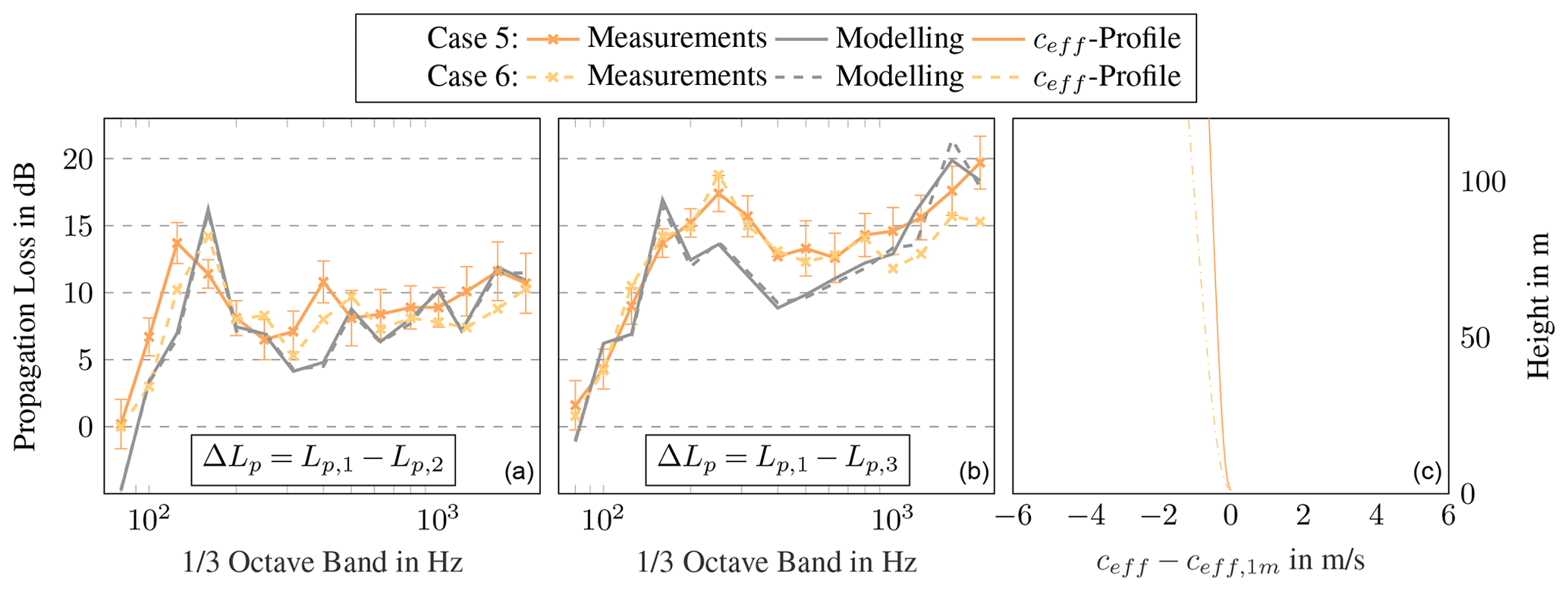
Figure A1 Comparison of measured and modelled propagation losses per one-third octave band for cases 5 and 6. (a) Propagation losses between Mic 1 (178 m) and Mic 2 (535 m), including standard deviation for measurement in case 5. (b) Propagation losses between Mic 1 (178 m) and Mic 3 (845 m), including standard deviation for measurement in case 5. (c) Normalised profiles of effective sound speed.