the Creative Commons Attribution 4.0 License.
the Creative Commons Attribution 4.0 License.
 | 01 Jun 2023
A comparison of eight optimization methods applied to a wind farm layout optimization problem
Nicholas F. Baker
Paul Malisani
Erik Quaeghebeur
Sebastian Sanchez Perez-Moreno
John Jasa
Christopher Bay
Federico Tilli
David Bieniek
Nick Robinson
Andrew P. J. Stanley
Wesley Holt
Andrew Ning
Selecting a wind farm layout optimization method is difficult. Comparisons between optimization methods in different papers can be uncertain due to the difficulty of exactly reproducing the objective function. Comparisons by just a few authors in one paper can be uncertain if the authors do not have experience using each algorithm. In this work we provide an algorithm comparison for a wind farm layout optimization case study between eight optimization methods applied, or directed, by researchers who developed those algorithms or who had other experience using them. We provided the objective function to each researcher to avoid ambiguity about relative performance due to a difference in objective function. While these comparisons are not perfect, we try to treat each algorithm more fairly by having researchers with experience using each algorithm apply each algorithm and by having a common objective function provided for analysis. The case study is from the International Energy Association (IEA) Wind Task 37, based on the Borssele III and IV wind farms with 81 turbines. Of particular interest in this case study is the presence of disconnected boundary regions and concave boundary features. The optimization methods studied represent a wide range of approaches, including gradient-free, gradient-based, and hybrid methods; discrete and continuous problem formulations; single-run and multi-start approaches; and mathematical and heuristic algorithms. We provide descriptions and references (where applicable) for each optimization method, as well as lists of pros and cons, to help readers determine an appropriate method for their use case. All the optimization methods perform similarly, with optimized wake loss values between 15.48 % and 15.70 % as compared to 17.28 % for the unoptimized provided layout. Each of the layouts found were different, but all layouts exhibited similar characteristics. Strong similarities across all the layouts include tightly packing wind turbines along the outer borders, loosely spacing turbines in the internal regions, and allocating similar numbers of turbines to each discrete boundary region. The best layout by annual energy production (AEP) was found using a new sequential allocation method, discrete exploration-based optimization (DEBO). Based on the results in this study, it appears that using an optimization algorithm can significantly improve wind farm performance, but there are many optimization methods that can perform well on the wind farm layout optimization problem, given that they are applied correctly.
- Article
(5885 KB) - Full-text XML
- BibTeX
- EndNote


Wind farm layout design presents a challenging and complex problem due to the variable nature of the wind and complex interactions between turbines through their wakes. Finding a good layout is critical because even relatively small improvements in energy conversion can translate to significant gains in revenue. Because the wind farm layout design problem is so complex, optimization algorithms are often used to help designers find good layouts. Wind farm developers and members of the academic community alike understandably struggle when attempting to select a wind farm layout optimization method: the numerous available methods differ in many ways, but the differences, affordances, and constraints of each method can be difficult to determine. The varying case studies, objectives, metrics, and author expertise between individual studies add enough variability that direct comparisons between methods in different papers are very difficult to make and yield uncertain results. To facilitate more objective comparisons between wind farm layout optimization methods, we provide algorithm comparisons where a common objective function was provided and each algorithm was managed by researchers with previous experience using them. These comparisons should aid wind farm developers and the academic community in selecting an appropriate optimization algorithm for their specific wind farm layout optimization applications. In the following few paragraphs we provide a high-level overview of optimization, present the types of algorithms available, and discuss each type's typical strengths and weaknesses, particularly as related to the wind farm layout optimization problem.
Optimization algorithms are intended to improve a design or process. At a minimum, they rely on receiving feedback in the form of a function output or real-time data set to control a set of inputs to the system that affect change in the output. For complex systems, such as a wind farm, the optimal design is difficult to determine because the design space is too large for exhaustive exploration using available methods. Therefore, designers use optimization algorithms to find good, if not globally optimal, designs efficiently, without an exhaustive search. There are many different optimization methods, but they fall into three general categories: gradient-based, gradient-free, and convex. Because wind farm layout optimization problems are not generally convex, convex methods are not applicable. We will discuss only gradient-based and gradient-free methods in the remainder of this work.
As their name implies, gradient-based methods rely on some knowledge of the slope, or derivatives, of the objective function (Belegundu and Chandrupatla, 2011). Gradient-based methods are often considered to be only local-search algorithms because, in their simplest form, they often just follow the slope to the nearest local optima. However, gradient-free methods are not limited to local search as they can be combined with global-search techniques. Gradient-based methods also scale very well to complex problems with many variables and constraints without an excessive increase in computational cost. Besides relying on derivatives, gradient-based methods also require that the objective function be smooth enough (Martins and Ning, 2021). These requirements make applying gradient-based methods to many black-box objective functions undesirable because the derivatives of black-box functions can only be obtained through finite differences. If finite differences are used, then the computational cost of calculating the derivatives can be high and the derivatives may have significant error (Gray et al., 2014). Determining the derivatives symbolically can be difficult or even impossible depending on the objective (Martins and Hwang, 2013). Algorithmic differentiation (AD) is a common and efficient solution to the problem of obtaining derivatives. In AD, the source code is differentiated line by line algorithmically and the resulting derivatives are exact (Griewank and Walther, 2008).
By contrast, gradient-free methods rely only on the objective function (Koziel and Yang, 2011), which makes applying gradient-free methods to black-box objective functions very simple. However, these methods must work without the knowledge of the shape of the design space that is available through gradients. Gradient-free methods may be either deterministic or heuristic. They may also be either global- or local-search algorithms (though even global-search algorithms often fail to find the true global optimum for complex and high-dimensional problems; Arnoud et al., 2019). Many gradient-free methods use multiple function evaluations (sets, points, populations, etc.) at each step to provide the information needed to determine the next step(s) in the optimization. Due in part to using a population or set of solutions at each iteration, gradient-free methods are often preferable for problems with many local optima (multimodal problems). However, gradient-free methods may require more function calls than gradient-based methods and do not usually scale well to problems with more than 30 design variables (Rios and Sahinidis, 2013).
To reduce the number of design variables and constraints, optimization algorithms may use re-parameterization (Serrano González et al., 2017; Stanley and Ning, 2019) or discretization (Mosetti et al., 1994; Grady et al., 2005; Turner et al., 2014). To help overcome the problem of local optima, optimization algorithms may be paired with global-search techniques, including (but not limited to) multi-start approaches (Guirguis et al., 2016), continuation methods (Mobahi and Fisher, 2015), or both (Thomas et al., 2022a). Occasionally, multiple optimization algorithms are combined in a hybrid approach to globalize the search of the design space with a global-search method and then speed up the refinement of the solution using a local-search method. A hybrid approach may combine gradient-free and gradient-based algorithms (as in the work of Réthoré et al., 2014) or two algorithms of the same type (as done by Yang et al., 2021). There is no one best optimization algorithm (Press et al., 2007). The choices of optimization algorithm(s) and peripheral method(s) are highly dependent on the problem and situation.
The characteristics of the wind farm layout optimization problem further complicate algorithm selection. The wind farm layout optimization problem has a highly multimodal design space (Stanley and Ning, 2019), which may lead us to use gradient-free methods. On the other hand, wind farm layout optimization problems may also have hundreds of design variables and thousands of constraints, which may lead us to choose a gradient-based optimization method with AD derivatives. In addition to these general considerations, each optimization method and wind farm design problem has unique characteristics that must be considered.
Numerous studies have applied various optimization algorithms to the wind farm layout optimization problem (see the comprehensive review by Herbert-Acero et al., 2014). Some of these studies try to provide a meaningful optimization algorithm comparison by comparing results on the same scenarios as previous studies, such as in Grady et al. (2005), Turner et al. (2014), and Zergane et al. (2018). However, correctly re-creating the objective function and other elements of previous studies is very difficult and prone to error. Exact duplication may even be impossible. Tracking the chains of studies to compare algorithms is also fairly difficult. Very few studies have directly compared multiple optimization algorithms in a single study (Brogna et al., 2020). The following few paragraphs provide a brief review of studies that have compared more than two optimization algorithms on a single wind farm layout optimization problem in a single paper.
Fischetti and Monaci (2016) compared three heuristic optimization algorithms (a subset of gradient-free methods). They used one commercial algorithm from IBM (IBM ILOG Cplex 12.5.1) with two different tunings, a self-made local-search procedure, and a self-made mixed-integer programming method. They tested on farms that were 3000 m by 3000 m with 1000–10 000 uniformly random potential turbine locations. They found that their self-made mixed-integer programming method outperformed the others in most cases.
Guirguis et al. (2016) compared a genetic algorithm (GA) (gradient-free), a hybrid algorithm made of a GA followed by a sequential quadratic programming algorithm (gradient-based), and an interior-point nonlinear programming algorithm (gradient-based). These algorithms were tested on farms with 10, 20, and 30 turbines with three different wind resources. The first wind resource had a single wind state, the second had multiple directions but a single wind speed, and the third had a distribution of both wind speed and direction. All algorithms were run 10 times for each problem with different random seeds. They found that the interior-point method outperformed both the GA and the hybrid method for all cases.
Baker et al. (2019) presented the results of a first set of wind farm layout optimization case studies under the International Energy Association (IEA) Task 37 Work Package 3. This was a blind study; participants did not see others' results prior to submission. Two separate studies were performed. The first consisted of three round farms, with 16, 32, and 64 wind turbines, for which the objective function was provided but participants in the studies applied whatever optimization algorithm they chose. The study included 10 submissions representing 9 optimization methods. Six of the submissions used gradient-based approaches, and the other four used gradient-free methods. At least the top four optimization algorithms for each wind farm were gradient-based methods. Resulting improvements from the provided baseline layout ranged from 2.93 % to 17.05 %. The second study consisted of a single wind farm with only nine turbines, but participants were free to use whatever wake and other models they chose and to select their optimization algorithm. Results of the second study were compared using a round-robin. The second study included five submissions, only one of which was gradient-free. The gradient-free method ranked at or just below the middle of the five for all cross-comparisons of the round-robin.
Brogna et al. (2020) compared eight different optimization algorithms on a single wind farm as an extension of their work presenting a wake model for use with complex terrain. The algorithms were applied to a wind farm in complex terrain with 25 turbines. Two of the algorithms in this study were gradient-based, and two of the remaining six were implemented by the researchers. The off-the-shelf algorithms were all from the MATLAB toolbox. A total of 10 runs were completed with each algorithm on 10 randomly generated starting points. The researchers tried doing a single-stage optimization using the final objective function, as well as a double-stage optimization where wake effects were ignored during the first stage and included during the second stage. Gradient-free algorithms dominated. The gradient-based algorithms performed near the bottom for the single-stage and worst for the double-stage. They found that their self-implemented algorithms performed the best on this problem.
Kunakote et al. (2022) compared 12 meta-heuristic algorithms (a sub-set of gradient-free algorithms) for wind farm layout optimization. They compared the meta-heuristic methods on four cases, all with the same 2 km by 2 km wind farm. The first case divided the farm into a 10 by 10 grid and allowed the final result to have 1 to 100 wind turbines and an extremely simple wake model. The second case was the same but with more accurate wake effects included. The third case set the number of turbines to 39 but kept the same placement grid and used the simpler wake model. The final study used 39 turbines on the same grid with the more accurate wake model. They found that the real-coded ant colony optimization performed the best on cases 1 and 2. The moth-flame optimization algorithm performed the best on cases 3 and 4.
While all of the above studies are useful and contribute to a deeper understanding of how various algorithms and types of algorithms perform on the wind farm layout optimization problem, they exemplify some of the difficulties of comparing algorithms for wind farm layout optimization. In some cases the same researchers managed all of the algorithms (Fischetti and Monaci, 2016; Guirguis et al., 2016; Brogna et al., 2020; Kunakote et al., 2022). While having the same people running each algorithm is helpful in some respects, many algorithms have unique attributes that may only be understood by people who have used them often and studied them deeply. It is hard to know whether the algorithms performed better or worse due to the users' experience or the algorithms themselves. In particular, it is interesting that in Fischetti and Monaci (2016), Guirguis et al. (2016), Baker et al. (2019), and Brogna et al. (2020), the authors found algorithms they either developed or coded themselves to perform the best. This is not to imply there was bias in the analysis. The problem formulation may have an impact on which algorithms perform well, and applying a range of algorithms well to the same problem requires a significant amount of work and expertise, sometimes even requiring restructuring the problem formulation. Two of the five studies discussed in detail (Guirguis et al., 2016; Kunakote et al., 2022) only investigated heuristic and meta-heuristic algorithms. Gradient-based algorithms have historically been discredited by researchers for application to the wind farm layout optimization (Herbert-Acero et al., 2014). All of the studies mentioned dealt with fairly simple wind farms in terms of size and constraints, though Brogna et al. (2020) took a great step toward realistic wind farm design by working with complex terrain. None of the studies done to date compare optimization algorithms on wind farm layout optimization problems with multiple discrete boundary regions or concave boundaries, and only one drew on different researchers to run the optimizations for each optimization algorithm.
The need for clear comparisons of optimization methods as applied to more complex and realistic wind farm design problems was part of the motivation for IEA Wind Task 37 to start a work package focused on collaborative case studies of wind farm design problems (IEA, 2021). The first set of wind farm design case studies (case studies 1 and 2) under this work package, and discussed previously, was published in Baker et al. (2019). These first case studies were designed to be introductory such that anyone could use them to get started in the field of wind farm layout optimization. The first two case studies were simple, mostly smaller, round farms for which all methods were relatively easy to apply. The second set of case studies, including case study 4 whose results are presented in this paper, are based on the Borssele III and IV wind farms. Among the additional complications of these case studies are non-convex boundaries, discrete regions rather than a single boundary, and more wind turbines (81 wind turbines in case study 4). The original request for submissions for case studies 3 and 4, and all accessory files, can be found in Baker et al. (2021).
In this work we describe eight different wind farm layout optimization methods and compare their performance using a relatively complex optimization scenario (IEA 37 WP 3, case study 4). While the original intent of the case studies was to run a blind study, with participants separate from the authors, the number of participants was fairly low, so the participants agreed to work together as co-authors on this paper. Each of the author-participants selected an optimization method so that they could work with, and focus on, methods in which they had the requisite experience and expertise. In several cases the methods were applied, or their application was directed, by the methods' originators. Our objective is to help the reader make a more informed optimization method selection by clearly comparing the pros and cons of a range of methods and presenting results from each method on a shared wind farm layout optimization case study with reasonable complexity and a provided objective function. We also hope to provide a set of high-quality wind farm layout optimization results to serve as benchmarks for other optimization methods. In the remainder of this paper we present our methods, including a description of the case to be optimized, the wind farm simulation approach, and a detailed description of the eight optimization methods included. We then provide results of the case study and optimization method analysis. We conclude with a brief summary and discussion of future work.
As mentioned in the Introduction, this paper describes eight different strategies used to optimize the same wind farm layout. The objective of this case study was to maximize the annual energy production (AEP) of a wind farm, based on the Borssele III and IV wind farms, by optimizing the placement of 81 wind turbines. The turbines are 10 MW machines with 198 m rotor diameters based on the IEA 10 MW reference wind turbine (Bortolotti et al., 2018). The wind farm boundary for this case study was split into five discrete regions, shown in Fig. 1. The presence of unconnected regions in the wind farm boundary can be challenging when an algorithm requires a continuous objective function or derivatives. The wind turbines can be placed in any of the five regions of the wind farm, but not between them, making the problem inherently discontinuous and non-differentiable.
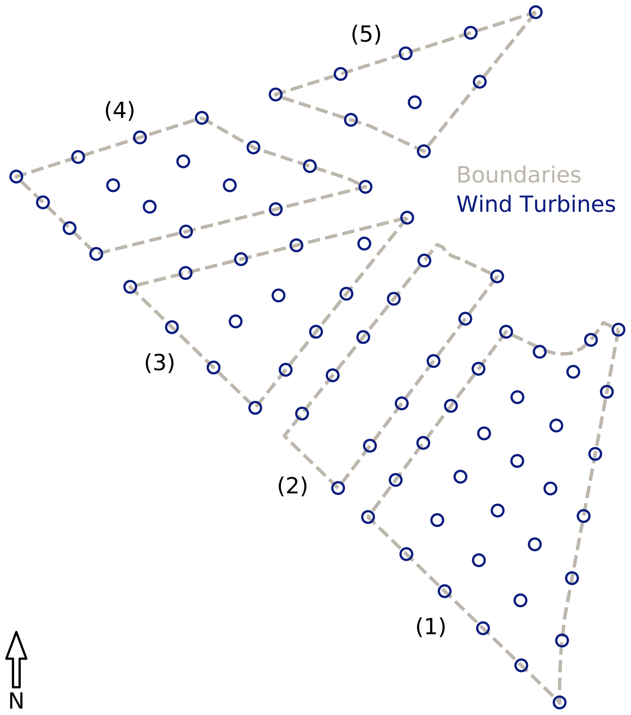
Figure 1An overhead view of the wind farm used for the case study, including the provided example wind farm layout. Numbers in parentheses indicate region numbers. Wind turbine markers' diameters are the rotor diameters.
We used a simple Gaussian wake model based on Bastankhah's Gaussian wake model (Bastankhah and Porté-Agel, 2016), and presented in the IEA case study 3 and 4 announcement documents (Baker et al., 2021), to calculate wind speeds at each turbine in the wind farm.
where ΔV is the velocity deficit, V∞ is the wind velocity without wake losses, is the constant thrust coefficient, d=198 is the rotor diameter, Δy is the distance from the center of the wake to the point of interest perpendicular to the wind direction, Δx is the distance from the turbine generating the wake to the point of interest in the wind direction, and σy controls the width of the wake. The value of σy is calculated as
where ky is a tuned variable based on turbulence intensity. We used ky=0.0324555 based on a turbulence intensity of 0.075 (Niayifar and Porté-Agel, 2016; Baker et al., 2021). The individual wake calculations were combined using the square-root-of-the-sum-of-the-squares method (Katic et al., 1986).
where NT is the number of wind turbines.
We chose AEP as the merit figure for the optimizations, with AEP defined as
where the power of each turbine k for each wind direction i and speed j is represented by Pijk, the probability of a given wind speed and wind direction combination is given by fij, and ND and NS represent the number of wind directions and wind speeds, respectively. The objective function can then be defined as
where Sij represents the spacing between turbine i and turbine j, [xi,yi] is the location of each turbine, and Ω is the set of all points in the defined boundary regions (see Fig. 1).
The objective function code was provided in the Python programming language, but some authors chose to re-implement the code in a different language. The wind resource, shown in Fig. 2, was divided into 360 different wind direction bins, and the wind speeds were assumed to follow a Weibull distribution, with 20 speed samples per wind direction. We increased the number of wind directions from the wind rose given in the original case study documents to make the problem more realistic. The wind speed probability distributions were unique in each direction. The complete wind rose definition is available in the supplemental data repository (see “Code and data availability” at the end of the paper). A more complete description of the case study prompt can be found in Baker et al. (2021).
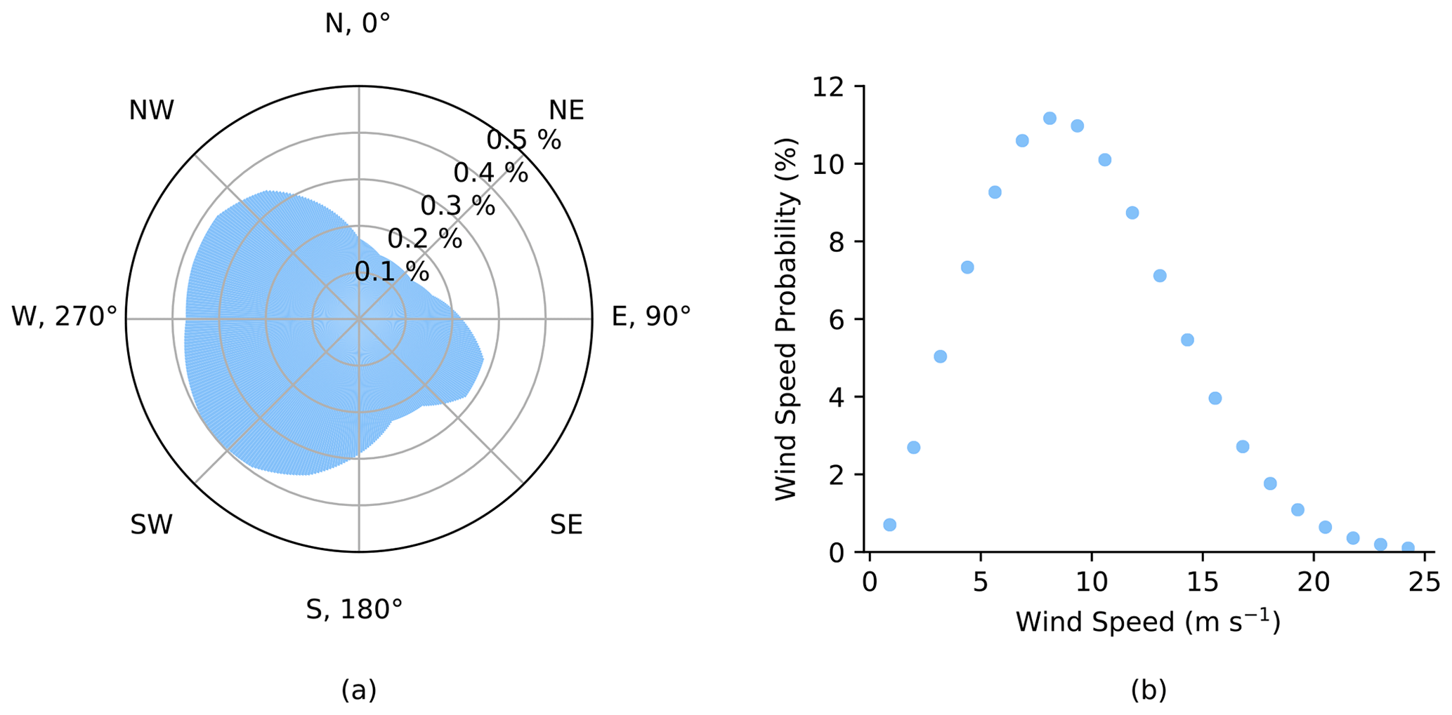
Figure 2The full wind resource used for evaluating the final wind farm layouts. (a) The wind direction probability (360 bins). (b) A representative wind speed probability distribution (20 bins). The wind speed probability distributions were based on a Weibull distribution and represent the probability of wind at each speed in a given wind direction.
We compared the results of the optimization algorithms using a range of metrics in an attempt to capture some of the trade-offs between the algorithms. The simplest comparison was based on the objective merit figure, AEP. We also compared the layouts using wake loss, a common metric that indicates how much potential energy conversion was missed due to wake effects. We calculated wake loss, Lw, as
where AEP* represents the ideal AEP that would exist if all of the wind turbines were exposed to the freestream wind. Because most of the algorithms were run on different hardware, we do not compare run time. However, to provide some comparison of computational cost, we report the number of function calls run during the optimization. There are many trade-offs in the wind farm layout optimization problem that cannot be captured in a measurable way. We have also provided pro and con lists to help the reader understand some of the more qualitative comparisons of the algorithms.
Although the objective was the same for all, each participant in this case study approached the problem from a unique perspective and with different methods. The rest of the Methods section includes brief explanations of the problem formulations and optimization techniques that each participant used to solve this wind farm layout optimization study. The included methods are as follows: sparse nonlinear optimizer with wake expansion continuation (SNOPT + WEC), discrete exploration-based optimization (DEBO), generalized pattern search (GPS), covariance matrix adaptation evolutionary strategy (CMA-ES), genetic- and gradient-based hybrid algorithm (GA-GB), add–remove–move greedy (ADREMOG), pseudo-gradient optimization (PG), and the discrete perturbation algorithm (DPA).
2.1 Sparse nonlinear optimizer with wake expansion continuation (SNOPT + WEC)
Despite the inherently multimodal nature of the wind farm layout optimization problem, gradient-based methods have been shown to provide excellent results (Fleming et al., 2015; Guirguis et al., 2016; Gebraad et al., 2017; Baker et al., 2019; Thomas et al., 2017, 2019, 2022a). One such method, particularly developed to overcome the local optima problem in the wind farm layout optimization problem, is called wake expansion continuation, or WEC (Thomas et al., 2022a). Because WEC is a higher-level process rather than a complete optimization algorithm, it relies on other optimization algorithms to function. We used the sparse nonlinear optimizer (SNOPT) because it is designed for nonlinear problems with many design variables and constraints (Gill et al., 2005). We will refer to this complete optimization method as SNOPT + WEC.
WEC was originally proposed by Thomas and Ning (2018), was refined and further tested by Thomas et al. (2022a), and has been shown by Baker et al. (2019) to perform well as compared with other approaches. WEC is a continuation method that requires a series of optimizations, similar to Gaussian continuation optimization as discussed by Mobahi and Fisher (2015). The WEC method makes use of the inherently Gaussian shape of the wake cross sections, as modeled using simple wake models like the one in this study. If the widths of the many Gaussian curves representing the wakes behind each turbine in each direction are increased while keeping the wake deficit (peak of the Gaussian curve) the same, the curves will combine in such a way that the Gaussian curves with lower peaks will essentially disappear, causing a smoothing effect on the overall design space that reduces the number of local optima. For WEC to work, a small adjustment must be made to the wake model that allows the user to manipulate the width of the wake cross section without directly impacting the wake deficit in the center of the wake. To use WEC with the wake model in this study we added a single coefficient, ξ, to the denominator of the exponential term of Eq. (1) as follows:
Values of ξ greater than unity provide a smoothing effect, which removes some local optima; when ξ equals unity, it no longer impacts the model. The first optimization uses a high value of ξ, and then ξ is decreased for each optimization in the series until ξ gets to 1. We used the values of ξ suggested by Thomas et al. (2022a) for our WEC series: 3.0, 2.6, 2.2, 1.8, 1.4, and 1.0. An example using a simple wind farm to demonstrate the impact of WEC on the design space is shown in Fig. 3. With fewer local optima, the gradient-based optimization algorithm is free to progress toward better layouts without getting stuck.
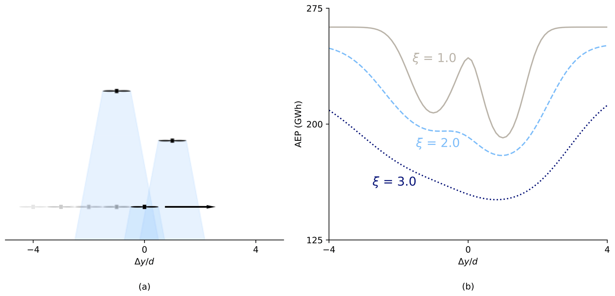
Figure 3The local optimum between the wakes disappears as the WEC factor increases. (a) Simple wind farm with three turbines, seen from above. Wind is from the top. Shaded regions represent the wakes but are not drawn according to any wake model. (b) The AEP for the wind farm in (a) as calculated using the provided simple Gaussian model with different values of the WEC factor, ξ, while moving the most downstream turbine in (a) across the wakes of the other two turbines.
We implemented a completely continuous and gradient-based version of the optimization problem. The model was developed and optimized in the Julia language (Bezanson et al., 2017), using algorithmic differentiation provided by the ForwardDiff.jl package (Revels et al., 2016) to calculate the derivatives. We set up and ran the optimization problem using SNOW.jl (https://github.com/byuflowlab/SNOW.jl, Ning, 2021). We scaled all partial derivatives to be ±1 with the exception of the boundary constraint derivatives, which we scaled to be between to reduce the impact of the boundary on the turbine locations while still ensuring that the boundary constraints were met.
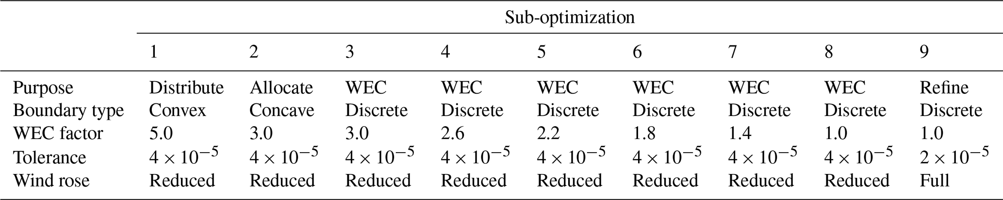
To determine how many turbines should be placed in each region, we used an initial boundary made of the convex hull of the provided boundaries to encourage even turbine distribution in the design space (see Fig. 4a). We used a higher WEC factor value for this initial sub-optimization to encourage rapid turbine distribution in the farm area. Following the optimization with the convex hull, we ran an optimization using an approximation of the concave hull to push turbines closer to feasible points (see Fig. 4b). The concave hull approximation used the following boundary points: (9361.5, 126.9), (10 363.8, 6,490.3), (6054.7, 8925.3), (7048.3, 9531.5), (8953.7, 11 901.5), and (107.4, 9100.0). At the completion of the optimization using the concave hull, turbines were assigned to their nearest region. Turbine-to-region assignments were kept constant for the rest of the sub-optimizations in the series. We used a relatively coarse wind rose discretization with the average wind speed in each of 100 directions for the initial sub-optimizations and WEC series. Once the WEC optimization series was complete, we ran a final optimization with the full wind rose (360 wind directions with 20 wind speeds in each direction as shown in Fig. 2) and ξ=1. The sub-optimization step purpose, boundary, WEC factor values, convergence tolerance, and wind rose discretization for each sub-optimization in the series are shown in Table 1.
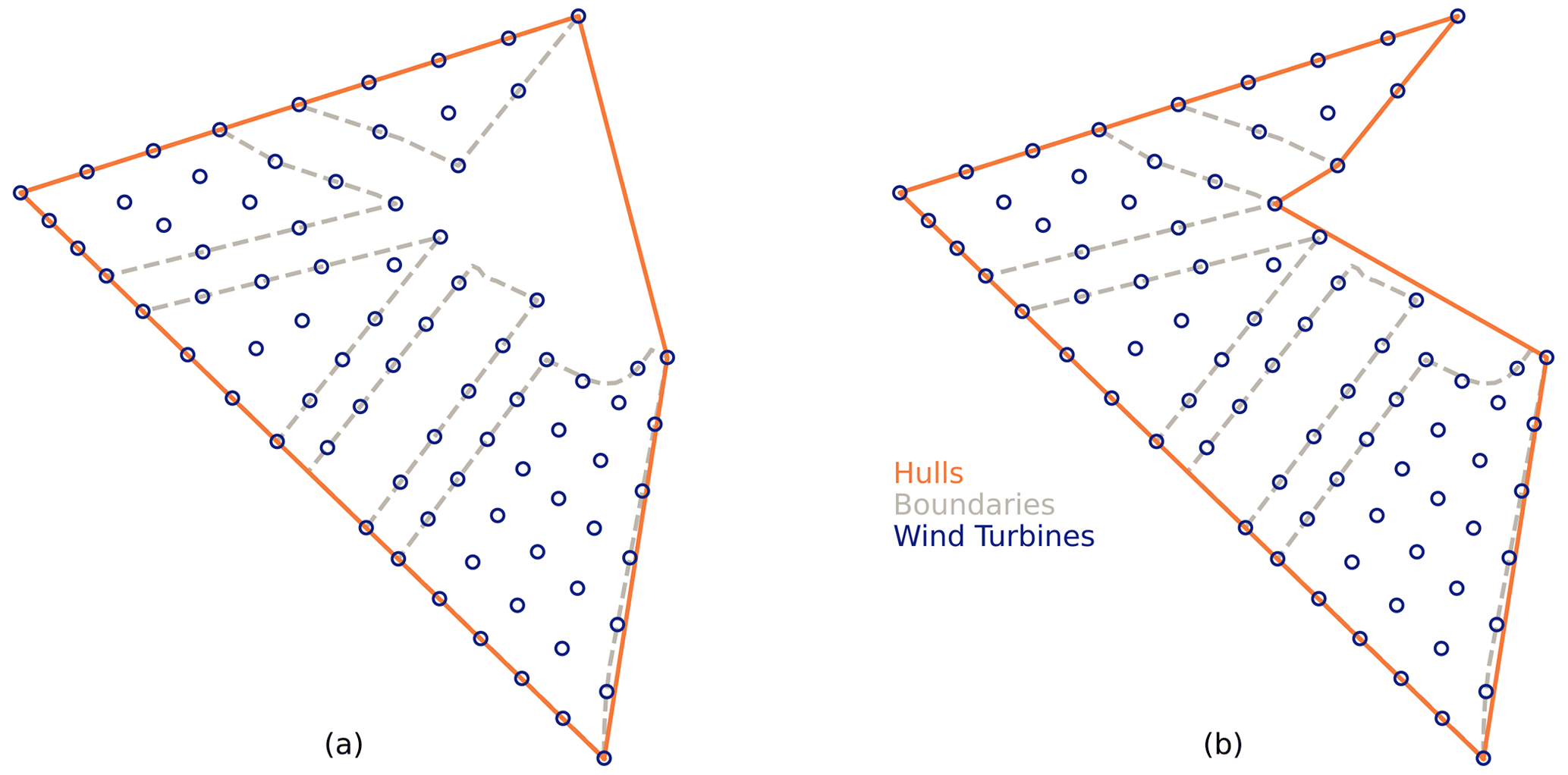
Figure 4The convex and concave hulls used for the SNOPT + WEC method. (a) The convex hull as used in sub-optimization step 1. (b) The concave hull as used in sub-optimization step 2. The labels apply to both (a) and (b).
Table 1Description of each sub-optimization for the SNOPT + WEC method.
Boundary and turbine spacing constraints were enforced using inequality constraints. The sign of the boundary constraint for each turbine represents whether the turbine is inside (negative) or outside (positive) of its assigned region. The sign is determined with a ray-casting algorithm based on the Jordan curve theorem (Press et al., 2007). For each turbine, a vertical ray is drawn and the number of intersections with its region's boundaries is counted. If the number of intersections is odd, then the turbine is within the boundary; if it is even, then the turbine is outside the boundary. The magnitude of a turbine's constraint value is equal to the distance from the turbine to the nearest point on the boundary of its assigned region. Thus, the larger the constraint value for a turbine is, the farther away from a feasible region it is. In order for this constraint method to be compatible with gradient-based optimization, it must be differentiable at every possible turbine location. To accomplish this, we used a soft-max function (instead of a traditional max and min function) when determining the magnitude of the constraint value.
We used the provided layout as a starting point and generated additional starting layouts loosely based on the approach taken by Stanley and Ning (2019). We evenly distributed about 45 % of the turbines on the boundary of the convex hull. Next we placed a regular grid of turbines with a row and column spacing of 4.25 rotor diameters in the farm centered inside the convex hull and rotated to a random angle between 0 and radians. Finally, we randomly removed turbines from the grid until there were only 81 wind turbines in the farm.
Some of the pros and cons of the SNOPT + WEC method are given in the following lists. Similar lists are provided for each algorithm. These lists are intended to help the reader understand why they may or may not want to use each method, but the lists are not exhaustive.
- Pros
-
- 1.
WEC allows local-search algorithms to move out of some local optima to achieve more globally optimal results than standard gradient-based optimization.
- 2.
WEC + SNOPT is scalable to large problems (especially when using exact derivatives).
- 3.
WEC + SNOPT is easily globalized through multi-start to improve search breadth and further avoid local minima.
- 4.
WEC + SNOPT requires relatively few function calls for optimization.
- 5.
WEC + SNOPT is free-form (no grid or other parameterization required).
- 6.
Open-source software is available with WEC already implemented in the wake models.
- 7.
WEC can be used with other optimization algorithms besides SNOPT.
- 8.
SNOPT works with linear and nonlinear functions and constraints.
- 9.
SNOPT has fast execution due to being in Fortran, with wrappers in Python and Julia for easy interface.
- 1.
- Cons
-
- 1.
WEC is invasive (requires simple edits to the wake model and its interface).
- 2.
WEC requires domain knowledge and testing due to possible negative interactions with some simulation models.
- 3.
SNOPT is limited to local search, even though WEC helps make it more global, so a multi-start approach is recommended.
- 4.
SNOPT is best used with exact derivatives, which can be challenging to obtain.
- 5.
SNOPT requires a license.
- 6.
Gradient-based optimization requires some expertise due to sensitivity to derivative scaling, starting points, parameters, constraint formulation, function smoothness, etc.
- 1.
2.2 Discrete exploration-based optimization (DEBO)
Discrete exploration-based optimization (DEBO) is a new algorithm developed specifically for this case study. DEBO aims to overcome two of the major difficulties of wind farm layout optimization. First, the 2D domain where turbines can be placed, Ω∈ℝ2, consists of unconnected regions. This feature makes the overall layout optimization problem both continuous and discontinuous. The problem is discontinuous because the optimization algorithm has to find the best way to divide the turbines among the different regions of Ω. The problem also has continuous characteristics because once the turbine division is made, the turbines may be placed continuously within their respective regions to optimize the AEP. Second, some of the regions are not convex, and the function to be minimized has many local optima throughout the search space. This last feature suggests that we should not rely solely on local methods because local methods alone may converge to poor local optima. Taking into account the combination of discontinuous and continuous characteristics, as well as the large number of local optima present in the wind farm layout optimization problem, we have developed a purely discrete exploration-based algorithm (DEBO) that includes both a greedy initialization procedure and a local-search refinement process.
-
Greedy initialization. The greedy procedure sequentially places the N turbines in an a priori defined domain where the wake losses can be minimized. This domain includes the boundaries of the different admissible domain. When the right number of turbines has been placed, the initialization stops.
-
Local search. The local-search method sequentially, and in random order, places each turbine in its discrete neighborhood until the AEP converges. The local-search method is inspired by classical stochastic gradient methods (Wasan, 1969)1. A stochastic gradient step consists of modifying only one randomly chosen coordinate of the parameters while the other coordinates are fixed. The DEBO method relies on the same principle; one, and only one, randomly chosen turbine is moved at each iteration. However, the DEBO method differs from classical stochastic gradient methods since DEBO is not gradient-based but relies on a discrete exploration region with a varying radius. The radius of the discrete exploration method is reduced each time the layout reaches a local minimum, i.e., when no discrete turbine displacement can improve the AEP. The DEBO method's local-search part also differs from the random search algorithm presented in Feng and Shen (2015). In Feng and Shen (2015), each turbine is moved randomly while it provides an increase in AEP, and then another turbine is randomly selected and moved randomly. This differs from DEBO because each turbine displacement is not required to belong to a particular neighborhood. Therefore, unlike the DEBO method, the random search algorithm presented in Feng and Shen (2015) has no guarantee to eventually stop. In addition, the presented version of the DEBO algorithm is highly parallelizable.
2.2.1 Formulation of the problem
We first define the layout of a wind farm F to be a sequence of turbine coordinates, (x,y), such that
where Nmax is the maximal number of turbines to be placed within the admissible domain Ω, and . We note that ⊕, the operation of concatenation between two sequences such as F, is defined as
We next define the power production of farm F for wind speed ws and wind direction wd as . The problem of interest, maximizing the expected power production of the wind farm (𝔼Wind), can then be formulated as
The proposed algorithm relies on a discretization of Ω in squares of dimension (dx,dy). The initial value of the meta-parameters (dx,dy) are set by the user. Using these parameters, we discretize the domain by defining Nx as
and Ny as
where , , , and represent the maximal and minimal values of x and y, respectively, in Ω. Using this discretization, we can define the discrete set of admissible positions, AΩ, as
where (nx,ny) represents a discrete point. To account for the turbine spacing constraint, we use the definition of a well-designed layout as shown in Definition 1.
Definition 1 (Well-designed layout). A layout F is dmin-well-designed if all its turbines are at least at a distance dmin apart from each other. Mathematically, a layout F is dmin-well-designed if the following mapping, WD, returns a true value, shown as ⊤. A false value is represented by ⊥.
Using Definition 1 and Eqs. (11), (12), and (13), we are able to state the combinatorial optimization problem as shown in Problem 1.
Problem 1 (Discrete problem). The discrete exploration-based optimization problem finds the 2Nmax variables corresponding to the locations of the Nmax turbines we want to place. This means solving the following problem:
such that
and
We are now ready to present the general method to compute an optimal layout using DEBO.
2.2.2 Presentation of the greedy part of the algorithm
The greedy part of the algorithm sequentially places the turbines in the admissible domain. To present the algorithm we introduce the definition of the interior border of the discrete admissible domain in Definition 2.
Definition 2 (Border). We represent the interior border of the admissible domain as ∂AΩ. A discrete point (nx,ny) of AΩ belongs to ∂AΩ if it is in AΩ and at least one of its neighbors is not. First, let us define the discrete neighborhood DN(nx,ny) of (nx,ny):
Using this definition of discrete neighborhood DN(nx,ny) of (nx,ny), we can define AΩ as the interior border of the admissible domain:
The greedy algorithm uses two sets.
-
First is a set of all the possible locations, LΩ, where a turbine can be placed. Therefore, at the beginning of the algorithm this set is equal to AΩ.
-
Second is a set of all potential locations, PΩ, where the next turbine can be placed. This set is a subset of LΩ.
The algorithm consists of initializing PΩ to ∂AΩ, placing the first turbine in the upper right side of the admissible domain, and repeating the following procedure:
-
updating the set LΩ by removing the points located at a distance inferior to dmin of the already placed turbines;
-
updating the set PΩ by removing its elements not in LΩ (i.e., the points located too close to the placed turbines) and by adding to this set all the points in LΩ located at a distance between dmin and the maximal turbine distance (dmax) of the last placed turbine;
-
placing a turbine in PΩ maximizing the AEP of the wind farm;
-
starting over until or until PΩ is empty: in the latter case, the algorithm failed to place the required number of turbines, and therefore, the algorithm starts over and this time PΩ is initialized as an empty set.
The complete greedy placement algorithm is presented in Algorithm 1, where card(F) is the current number of turbines in F.
Algorithm 1GreedyInitialization.
2.2.3 Discrete local-search exploration
The discrete local-search method starts from the layout obtained after the greedy algorithm. The greedy algorithm provided a reasonably good layout based on a not-so-coarse discretization of the domain, allowing the computations to be numerically tractable. The local-search part of the algorithm aims at getting closer to a continuous approach while keeping the discrete part of the algorithm tractable. To describe the local-search method, we define a neighborhood as in Definition 3. This neighborhood divides a square of length L centered at (x,y) into squares of size located in the admissible domain Ω.
Definition 3 (Neighborhood). We note that is the neighborhood of the point coordinate (x,y) defined as follows:
We are now ready to describe the principle of the local-search algorithm. The local-search method randomly moves each turbine in its discrete neighborhood in order to maximize AEP. The local displacements of the turbines are computed until convergence; that is to say, each turbine is located at the best possible spot of its discrete neighborhood. When convergence is reached, the length L of the neighborhood is decreased and we start the next set of sequential turbine displacements. The algorithm stops when L is small enough. The complete description of the local-search algorithm is given in Algorithm 2.
Algorithm 2LocalSearch.
At this point, it is important to emphasize that this local-search algorithm always converges. Indeed, for a given L, any turbine initially placed at p0 can only be moved to a position in the set . The admissible domain Ω being bounded, this set contains a finite number of elements. Therefore, for a given L, the set of all possible layouts is also a finite set corresponding to the Cartesian product of Nmax finite sets. Moreover, a turbine displacement is performed only if the resulting AEP is strictly greater than the current one. Therefore, in the worst case, the algorithm will test all possible layouts by always finding a turbine to move that increases the AEP. However, because this set is finite the algorithm will eventually stop. In practice, convergence is met in a few iterations.
2.2.4 Complete algorithm applied
The complete algorithm consists of using the greedy part to find a first reasonably good layout and then using the local-search algorithm with the output of the greedy algorithm as the initial layout. The complete DEBO algorithm as used in the presented case study is given in Algorithm 3. Visualizations of each part of the DEBO algorithm are provided in Fig. 5.
Algorithm 3Layout optimization algorithm.
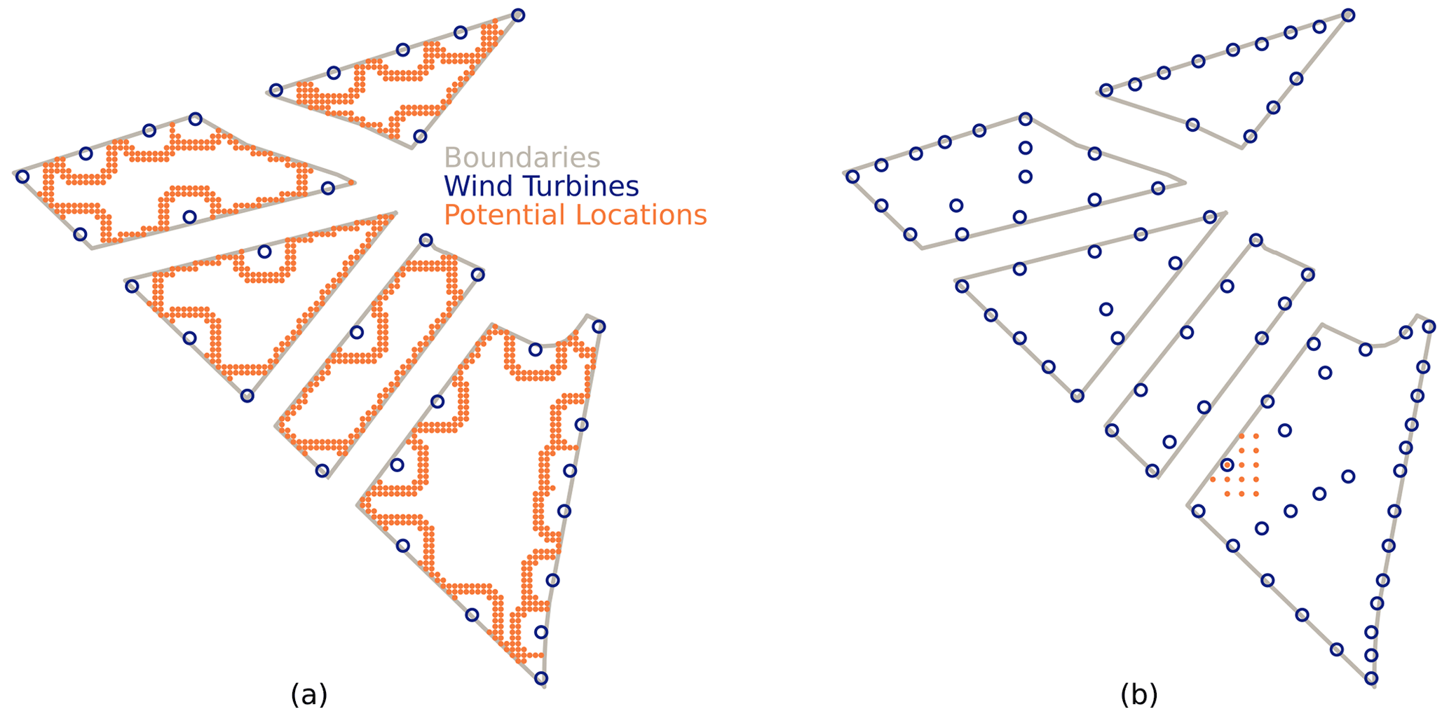
Figure 5Visualization of the two phases of the DEBO algorithm. (a) An iteration of the greedy part of the DEBO algorithm. Potential locations are candidates for the next turbine's location. (b) Part of an iteration of the local-search portion of the DEBO algorithm for refining the position of one turbine. Potential locations are the discrete neighborhood of the turbine to be moved. Labels in (a) also apply to (b). Turbine markers are to scale with diameter equal to the turbine rotor diameter.
Some pros and cons of DEBO are as follows.
- Pros
-
- 1.
No gradients are required (i.e., wake model can be considered as a black box).
- 2.
It can handle unconnected and non-convex boundary constraints.
- 3.
There is no strong dependence on the initialization, so it can be run just once. The exploration procedure is random enough to efficiently explore the search space.
- 4.
It is easy to parallelize.
- 5.
Parameterization is quite simple and does not require much optimization theory knowledge.
- 1.
- Cons
-
- 1.
It requires fast AEP computation due to the high number of AEP evaluations.
- 2.
It is a new method, made specifically for layout optimization, so there is little known about its general performance.
- 3.
There is no documentation yet outside of this work.
- 1.
2.3 Generalized pattern search (GPS)
Generalized pattern search (GPS) is a common gradient-free deterministic optimization algorithm. Versions of this algorithm are typically found within commercial wind farm software, but the results generated here are based on MATLAB’s pattern search (part of the Global Optimization toolbox; MathWorks, 2020), which is one implementation of the GPS method.
The GPS algorithm moves each of the NT turbines individually based on a set of pattern vectors that represent unity vectors for each of the 2NT dimensions of the search space. The step size is changed iteratively throughout the optimization. Initially, larger step sizes are tested. Step sizes are decreased later in the optimization, resulting in minimal turbine movements at the end.
The site boundaries and minimum turbine spacing requirements are implemented using a combination of linear and nonlinear equality and inequality constraint formulations and a pre-made binary (0 for feasible, 1 for infeasible) penalty grid with a resolution of 5 m. This allows the turbines to move between the discrete boundary regions but results in a strong enforcement of all constraints right from the start of the optimization. The binary constraint approach can be more practical and faster than other methods (e.g., a ray-casting algorithm) when the site has a complicated (i.e., many vertices in the boundary), non-convex shape or many small exclusion zones (which may result from unexploded ordinance and other sources). In each iteration, a penalty value is interpolated for each turbine location. The sum of the penalties is used as an equality constraint (i.e., the sum should be equal to zero to indicate a feasible layout). In addition, if the sum is not zero, a fixed energy yield penalty of 50 % of the average production of a single turbine is applied to assure that infeasible layouts are also characterized by a poor performance.
The initial layout used for the optimization is a manual adaptation of the baseline layout, where more turbines are moved to the boundaries to increase the number of turbines with freestream conditions given the site-specific wind rose. Such “perimeter” style layouts are generally expected to yield a higher energy production for single wind farms and reflect common practices in wind farm layout design.
Some pros and cons of GPS are as follows.
- Pros
-
- 1.
It is a simple algorithm that is well documented and quickly implemented.
- 2.
No gradients are required (i.e., wake model can be considered as a black box).
- 3.
There is no need to modify the wake model implementation.
- 4.
It can handle multi-parcel net areas with non-convex site boundaries where turbines can move between discrete regions throughout the optimization.
- 5.
Internal separation of objective and nonlinear penalty function evaluations reduces the number of objective function calls.
- 1.
- Cons
-
- 1.
The MATLAB implementation used here requires a license (including an additional license to use parallel features).
- 2.
Some experience in wind farm layout design is required to provide a good initial layout to ensure algorithm performance.
- 3.
Lower performance is expected when starting from a random initial layout given the simple but hard penalty implementation used here.
- 1.
2.4 Covariance matrix adaptation evolutionary strategy (CMA-ES)
The covariance matrix adaptation evolutionary strategy (CMA-ES) implementation discussed in this paper is based on the publicly available pyCMA library (Hansen et al., 2019). CMA-ES is a gradient-free stochastic optimization algorithm that works by adaptively increasing or decreasing the search space for the next generation, changing the means and standard deviations of a multivariate normal distribution (the covariance matrix) where new solutions (layouts) are sampled (Ha, 2017). Pairwise dependencies between the variables in the distribution are represented by the covariance matrix.
The problem is formulated as the maximization of a fitness function that results from subtracting penalties from the net annual energy yield. The penalties are directly proportional to the sum of the distances between wind turbines and their closest feasible point (observing the minimum inter-turbine spacing and being within the boundaries of a parcel). Analytical functions are used to calculate the distances to the closest feasible point for both constraints. Furthermore, each penalty value is multiplied by a dynamic scaling factor that is a function of the iteration number. The scaling factors resemble logistic functions of time. These functions enable the constraints to be slowly enforced. The algorithm is then free at the beginning to explore infeasible solutions to maximize AEP and converge toward feasible solutions afterward. This formulation enables the algorithm to find the best distribution of turbines among the different site parcels and minimize wake effects simultaneously.
Some pros and cons of CMA-ES are as follows.
- Pros
-
- 1.
It is available in an open-source library.
-
It is an easy-to-use API to configure and customize the optimization algorithm.
- 2.
No gradients are required.
- 3.
It is easy to parallelize, as multiple solutions are evaluated in every iteration.
- 4.
It has a good design space exploration ability, likely to get close to global optimum.
- 5.
It can handle complex multi-region non-convex site boundaries.
- 6.
All runs from random initial layouts converge to layouts with similar AEPs (i.e., consistently finds comparably optimal layouts).
- 7.
Population size is independent of problem size (number of design variables).
- 8.
Fitness function acts as a black box with inputs and outputs.
- 1.
- Cons
-
- 1.
Nonlinear constraints have to be handled with penalty functions.
- 2.
There are no guidelines to scale penalty functions against energy yield.
- 3.
Requires many (≈104) function evaluations (or relatively fast fitness functions).
- 1.
2.5 Genetic- and gradient-based hybrid algorithm (GA-GB)
For the genetic- and gradient-based hybrid algorithm (GA-GB), the optimization problem was formulated using a sequential hybrid approach implemented in Python. This hybrid approach uses both a gradient-free genetic algorithm and a gradient-based sequential quadratic programming algorithm, as shown in Fig. 6. This figure shows the optimizers in rounded blue boxes, which feed and receive the data shown in off-diagonal gray boxes to the analysis components in the on-diagonal green boxes.
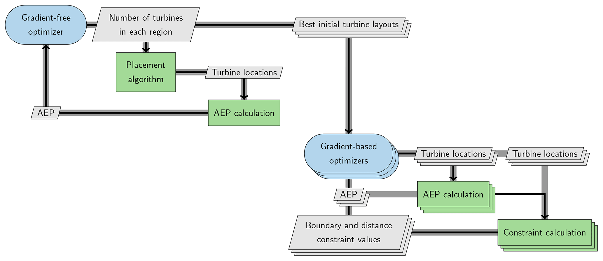
Figure 6Extended design structure matrix (Lambe and Martins, 2012) for the GA-GB optimization problem.
We first use a genetic algorithm (GA) implemented in OpenMDAO (Gray et al., 2019) to find the best initial layouts. The number of turbines in each region is a design variable exposed to the GA (i.e., in this case there are five design variables controlled by the GA). Then, a placement algorithm is used, which places most of the turbines for that region equidistantly along its border, with the remainder of the turbines inside the region, offset from the boundary. After 200 GA iterations with a population size of 30, we take the 20 turbine layouts with the highest AEP values and use each one of those layouts as the starting point for individual gradient-based optimizations. We use the SNOPT (Gill et al., 2002) optimization algorithm wrapped in pyOptSparse (Wu et al., 2020) to locally maximize AEP while controlling the turbine locations subject to boundary and spatial constraints, though any gradient-based optimizer can be used. Derivatives were obtained using finite differences. The resulting layout with the highest AEP value from these local optimizations is taken as the globally optimal layout.
A conventional gradient-based optimizer would have trouble exploring the discontinuous and multimodal design space created by the multiple discrete regions. This hybrid approach solves that issue by resolving those discontinuities using the GA. Smoothing the local design space and implementing analytic derivatives could greatly reduce the computational cost, but this increases developer time cost. Users of this method can choose to spend additional computational expense to fine-tune results at the local optimization level or they can explore the global design space more by increasing the number of iterations taken by the gradient-free method.
Some pros and cons of GA-GB are as follows.
- Pros
-
- 1.
GA-GB requires no modifications to the wake or farm calculations.
- 2.
Users can customize how much computation time to use on both the gradient-free and gradient-based processes.
- 3.
The method makes no assumptions about the number of parcels or turbines.
- 4.
GA-GB fully separates the discrete and continuous problems to remove optimizer complexity required for mixed-integer problems.
- 5.
The method can run on a personal computer and does not require supercomputing resources.
- 6.
GA-GB is agnostic of the wake modeling type used in that it does not require modification or knowledge of the wake model.
- 7.
Arbitrary linear and nonlinear constraints can be handled by the gradient-based optimization process.
- 8.
Both the gradient-free and separate instances of the gradient-based processes are embarrassingly parallelizable.
- 1.
- Cons
-
- 1.
The method does not directly take advantage of any physical relationships of the wakes, wind directions, or parcel orientation.
- 2.
Reaching multiple locally optimal layouts is straightforward using GA-GB, but finding the global optimum is not guaranteed.
- 3.
The sequential nature of the hybrid optimization approach means we cannot realize gains found by simultaneously changing the number of turbines in the regions and moving the turbine layout.
- 4.
SNOPT is best used with exact derivatives, which can be challenging to obtain.
- 5.
SNOPT requires a license.
- 1.
2.6 Add–remove–move greedy (ADREMOG)
Add–remove–move greedy (ADREMOG) is a discrete, heuristic greedy approach to wind farm layout optimization (Tilli, 2019). It makes use of a surrogate model, the pre-averaged model (PAM), to qualitatively assess the AEP, thereby speeding up optimization algorithms.
The PAM is a function that represents the expected power loss due to the wake of a turbine at given points in its surroundings. Figure 7 shows the PAM used in this case study. To derive the expected power loss at some point, we assume that a fictitious turbine is placed at the point. The fictitious turbine then experiences a wake loss due to the presence of another turbine at the center of PAM. PAM computes the expected loss of the target turbine by averaging over the wind resource. This approach can be used to estimate the quality of a layout in terms of energy yield. First, the expected power loss of each turbine in a given layout is obtained by summing up the individual contribution of the surrounding turbines. Next, the total AEP estimate is calculated by removing the energy loss of all the turbines from the theoretical energy production in the absence of wakes.
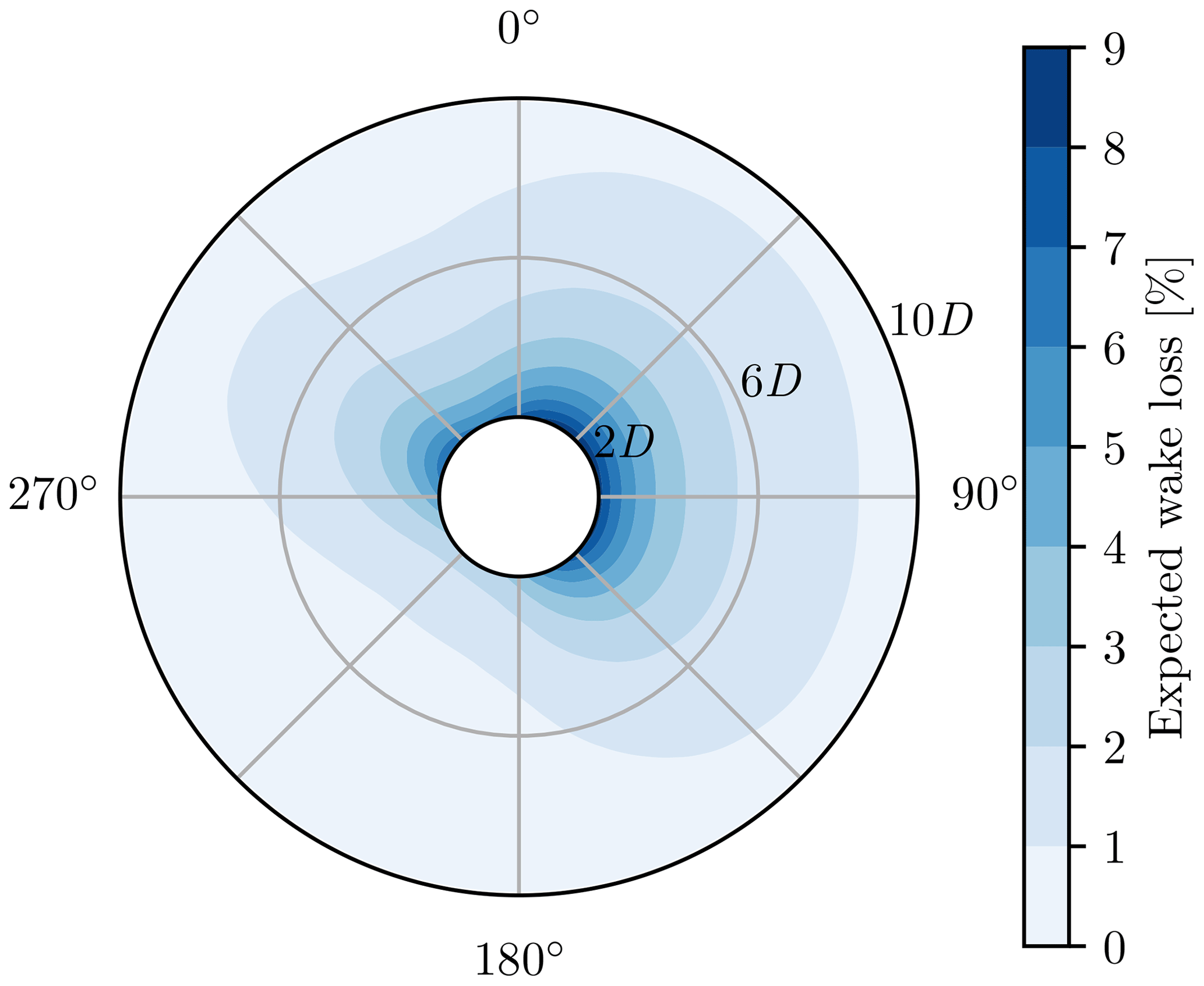
Figure 7Representation of the PAM calculated using the case study inputs. In this figure, D represents the rotor diameter.
The correlation between the AEP calculated by the PAM and by the traditional assessment methods is not exact. The PAM relies on the superposition of power losses, whereas traditional methods rely on the superposition of wake deficits. Nevertheless, the PAM is suitable for assessing relative AEP differences between layouts. Furthermore, the PAM allows us to run wake simulations and average the turbines' power output over the wind rose only once during the whole optimization procedure. Using the PAM, we can model wake-mixing effects by superposition of the power losses, which opens up the possibility of precomputing expected power losses among turbines. We can then use that information to generate layouts.
To precompute wake losses, we first create a finite set of possible positions within the wind farm boundaries. Afterward, we generate the PAM on a coarse polar grid. PAM is then centered in each possible position to obtain by interpolation the expected wake loss at the other spots.
To generate layouts, we feed ADREMOG with the precomputed power losses. The optimization procedure begins with a constructive stage. During this phase, ADREMOG iteratively adds a turbine to the layout where the loss associated with that added turbine is minimized. This stage starts by randomly placing the first turbine in one of the possible spots, and it terminates when the desired number of turbines is reached. The constructive stage is followed by the readjustment stage, where each turbine is removed from the layout and moved to a greedier position if it exists. ADREMOG terminates when a stable layout is reached.
ADREMOG solves an unconstrained optimization problem. The possible positions are selected before ADREMOG is launched, which ensures that all the turbines are enclosed within the wind farm boundaries. Also, compliance with proximity constraints is guaranteed by a static penalty. In particular, if a turbine does not respect the minimum distance, its expected power loss is replaced with an infinite loss. This ensures that ADREMOG selects a feasible spot when changing the layout.
As the placement of the first turbine impacts the quality of the final layout, multiple initial positions are investigated, which results in the creation of different layouts. The number of initial placements tested is chosen empirically. Because the AEP estimate from the PAM is only an approximation, each layout created is assessed with the traditional AEP calculation method to determine the best one found.
Some pros and cons of ADREMOG are as follows.
- Pros
-
- 1.
Combining PAM with ADREMOG results in a fast algorithm that allows
- 1.
exhaustive multi-start if desired,
- 2.
rapid preliminary layout generation, and
- 3.
cheap preprocessing.
- 1.
- 2.
PAM can be combined with optimization methods other than ADREMOG to speed them up.
- 3.
ADREMOG is easy to implement; it is simple.
- 4.
ADREMOG greedily selects the best position for turbines irrespective of the wind farm region. Therefore, it is particularly suitable for distributing the turbines among disconnected boundary regions.
- 1.
- Cons
-
- 1.
ADREMOG gets trapped easily in local optima. Therefore, a multi-start approach is suggested.
- 2.
PAM is a surrogate model. Therefore, final layouts need to be evaluated with a standard AEP calculation method to determine their actual wake energy loss.
- 3.
ADREMOG does not fully reach local optima due to the use of a surrogate model and space discretization. Nevertheless, improvements obtained when postprocessing the final layouts with pseudo-gradients (see Sect. 3.7) are minimal, suggesting that ADREMOG gets close.
- 4.
ADREMOG is too time-demanding if not employed in combination with PAM.
- 1.
2.7 Pseudo-gradient optimization (PG)
The pseudo-gradient (PG) optimization method is a heuristic technique for continuous optimization. The technique is described in detail by Quaeghebeur et al. (2021). Essentially, quantities similar to gradients are calculated from the basic quantities that need to be calculated for AEP calculations anyway, such as velocity deficits for a given wind direction and wind speed. These are then used as gradients would be, in a gradient-following-style approach.
The concept of pseudo-gradients is illustrated in Figs. 8 and 9. Figure 8 shows four types of pseudo-gradients for a simple case with a single wind direction and a disc-shaped site. Note their mostly parallel or perpendicular orientation relative to the wind direction. The first three types of pseudo-gradients try to reduce wake effects by moving waking and waked turbines away from each other, whereas the last type tries to reduce wake effects by moving turbines perpendicular to wind directions to get turbines outside of the wake(s) impacting them. Figure 9 shows the same four types of pseudo-gradients but now for a nontrivial wind rose. These are obtained by averaging the pseudo-gradients over all wind speeds and directions.
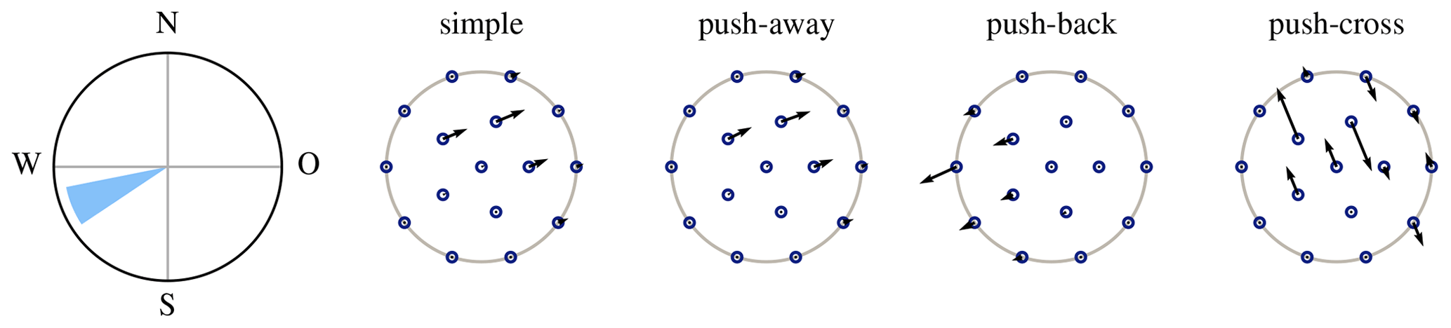
Figure 8Pseudo-gradient vectors associated with a single wind direction for the IEA Wind Task 37 case study 1 initial layout. (Reproduced from Quaeghebeur et al., 2021, which contains further details.)
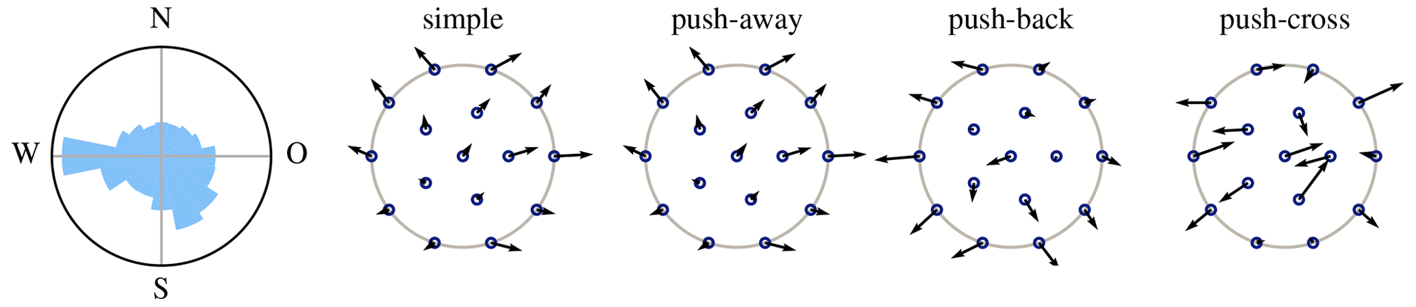
Figure 9Pseudo-gradient vectors for the IEA Wind Task 37 case study 1 initial layout and wind rose. (Reproduced from Quaeghebeur et al., 2021, which contains further details.)
The algorithm needs to start from an existing, initial layout. We have tested two approaches for determining an initial layout. The first, based on a hexagonal grid, is described below. The second uses the ADREMOG algorithm described in Sect. 2.6. The hexagonal-grid approach generates a hexagonal grid of turbines, with inter-turbine spacing maximized while fitting the number of turbines required in the site. The orientation and offset of the grid was determined by random sampling. From experience, it became clear that a sufficient number of turbines on the border is necessary to obtain a well-optimized layout. Therefore, the site was enlarged when determining the inter-turbine spacing. The turbines that fell outside of the actual site boundaries were moved to the closest point on the boundary. Any turbine distance constraint violations were then fixed by moving affected turbines away from each other. The site enlargement factor is an algorithm parameter, which can be used to influence the proportion of boundary vs. site-internal turbines.
The PG optimization itself tests three pseudo-gradient types and two step sizes (“smaller” and “larger”) concurrently. All are evaluated and the one with the lowest wake loss percentage (highest AEP) is selected to be used in the next iteration. If the “smaller” (“larger”) step size is chosen, the step size will be scaled down (up) for the next iteration. This scaling introduces an adaptive element to the algorithm that aids convergence. The initial step size multiplier and scaling factors are parameters of the algorithm.
It is possible that the wake loss percentage increases in this setup if the layout resulting from all three layouts is worse than the layout the update step is applied to. Therefore, the best layout encountered over the optimization run is chosen. There are two stopping criteria.
-
A maximum number of iterations can be set.
-
The wake loss percentage of the currently selected layout cannot exceed the best value encountered by a certain factor. This factor decreases with the number of iterations, making the criterion stricter over time.
Some pros and cons of PG are as follows.
- Pros
-
- 1.
On a per-run basis, the presented approach is computationally efficient relative to gradient-based approaches (no need to calculate analytical or numerical gradients) or meta-heuristic-based approaches (only a single or a few solutions are tracked every iteration). This efficiency creates specific possibilities.
- 1.
Use a shotgun approach to optimization: apply the algorithm for a relatively huge number of starting layouts.
- 2.
Use it when studying the impact of other considerations such as robustness studies, which typically require a large number of repeated optimization runs.
- 3.
Use it as a cheap pre- or postprocessor for other optimization approaches.
- 4.
Use it for interactive human-in-the-loop design.
- 1.
- 2.
It does not require discretization of the design space.
- 3.
Its simplest variant can be used for any wake model (including computational fluid dynamics models), and the other variants can be used whenever wake effects can be attributed to individual waking turbines (such as with typical engineering wake models).
- 4.
The concept behind it is flexible in the following ways.
- 1.
The steps moving turbines used in the pseudo-gradient-based approach can also be used as steps in meta-heuristic approaches, replacing the typically more random steps used there.
- 2.
Appropriate pseudo-gradients can be formulated for other concerns and aspects, such as the impact of bathymetry on substructure cost and cable layout.
- 1.
- 5.
An open-source implementation exists with a Python interface and efficient vectorized code.
- 1.
- Cons
-
- 1.
The approach is prone to getting trapped in local optima. Therefore, it is suggested to use a multi-start approach or combine it with techniques such as wake expansion continuation (e.g., Sect. 2.1).
- 2.
The heuristic nature of the approach “throws away” information available to true gradient-based approaches. Therefore we generally expect that, starting from an identical starting layout, gradient-based approaches will find better optimized layouts. (PG optimization is capable of investigating more starting layouts for equal computational cost.)
- 3.
While the adaptive nature of the algorithm lessens the need for semi-manual parameter tuning (initial step size and step multipliers), the quality of the optimized layouts can be substantially affected by parameter selection.
- 1.
2.8 Discrete perturbation algorithm (DPA)
The discrete perturbation algorithm (DPA) is a simple but effective gradient-free optimization method used in industry. The algorithm is based on a discretization of the design space with turbine locations tested by both directed and random perturbations from existing turbine locations. The algorithm proceeds as follows.
- 1.
Determine the smallest bounding rectangle that can contain all possible locations of the turbines (i.e., a rectangle containing the site boundary) and any wind resource information.
- 2.
Create a grid at a user-defined resolution, usually between 10 and 50 m.
- 3.
Determine whether each point in the grid is a legal turbine position (i.e., is it inside the site boundary and away from houses, roads, etc. as specified in the geographic information system layers). If the point is legal, add it to a 1D list of legal turbine positions for the current turbine layout.
- 4.
Using the wind resource information, order the list from highest wind speed to lowest. This creates a continuous 1D sorted list of turbine positions for the optimizer to work with rather than a 2D, fragmented, unsorted search space. In the unlikely case that the wind resource is uniform across the wind farm, this sorting step will not do anything. The purpose of sorting by wind resource is merely to avoid turbines jumping to positions which are significantly worse than their current position in terms of free-stream wind minus wake effects.
- 5.
Repeat steps 1 to 4 for each turbine layout so that there is a sorted list of legal positions for each turbine layout.
- 6.
Make sure the starting layout is legal. If it is not legal then make a legal layout from scratch (one way is to loop through the sorted list going from windiest to least windy while respecting the various constraints listed in step 8 – this means that the starting layout is already as windy as it can be but needs to be spaced out to find the optimal trade-off between wakes and resource).
- 7.
Test starting layout (for energy including wakes and all other losses) and keep a record of the net energy per turbine.
- 8.
Perturb the layout so that each turbine has a new legal position that respects the geographic information system constraints as well as noise, visual, shadow flicker, and inter-turbine spacing constraints (circular, elliptical, or sector-wise as defined by the user). Two types of perturbation are available.
- 1.
The priority is to jump to a better location from our sorted list of legal positions. However, we only jump to places that are higher in the list or whose wind speed is greater than the turbine’s current waked wind speed plus some small tolerance (a different but similar heuristic is used for the levelized cost of energy but from now on we will just talk about energy optimization). We make a few dozen attempts to jump to a new location, but if that is not working out (due to spacing, noise, etc.), then we try perturbation approach 8b.
- 2.
Random perturbations of the order of the grid spacing are used to sample legal positions. The aim of this is to allow the turbines to fine-tune once they find there are no big jumps to be made. However, if a position opens up, there is no reason why this turbine cannot go back to making big jumps. Sometimes there is another turbine already in the way for this iteration. If a successful random perturbation was made in the last step, then the same vector is used for this one to allow momentum in moving to a better location.
- 1.
- 9.
Test the perturbed layout. If the net energy is higher, then accept the perturbed layout as the new starting layout and go to step 8 (this almost never happens but can happen right at the start of an optimization).
- 10.
Look at the net energy results for each turbine. If the net energy given by the perturbed position is lower, then move this turbine back to its unperturbed position. If all turbines get moved back, then go to step 8.
- 11.
Test the layout again. It is possible that turbine 1 may have only appeared to be doing better because turbine 2 had been perturbed to a worse location. With the return of turbine 2, the last move of turbine 1 may no longer be a good move.
- 12.
Loop through steps 9 to 11 a maximum of three times before giving up and going to step 8.
- 13.
Repeat steps 8 to 11 for as long as patience or time allow; the algorithm has no good stopping condition and tends to continue improving indefinitely.
Some pros and cons of DPA are as follows.
- Pros
-
- 1.
It is simple to use and implement.
- 2.
It can be easily adapted to a wide range of constraints and objective functions.
- 3.
It can be used with any wake model, given sufficient resources.
- 1.
- Cons
-
- 1.
It requires discretization of the design space.
- 2.
There are no clear stopping criteria.
- 3.
There is no publicly available implementation, documentation, or publication outside of this work.
- 1.
Final layout metrics are provided in Table 2. The optimized AEP values of the best layouts found with each algorithm range from 2905.646 to 2913.221 GW h, representing improvements over the provided layout of 1.91 % to 2.18 %. The wake loss for the optimized layouts range from 15.486 % to 15.694 %. The total number of function calls used by each algorithm ranged from 97 930 to about 1 000 000. However, the function call comparison is tenuous at best due to the use of surrogate models, which run much more quickly than the regular model, by ADREMOG, as well as the use of a reduced wind resource during optimization by SNOPT + WEC. PAM runs much more quickly than the provided objective function. The function call counts reported for ADREMOG are estimated based on the relative run time for function calls of PAM as compared with the provided objective function. The actual function call counts to PAM were much higher. The run times are not included in this section to avoid confusion because the run times are not very comparable due to different hardware, different numbers of cores, and different programming languages used for some methods. Run time is discussed in each subsection on algorithm-specific results.
Table 2Optimization method comparison on a range of metrics and attributes.
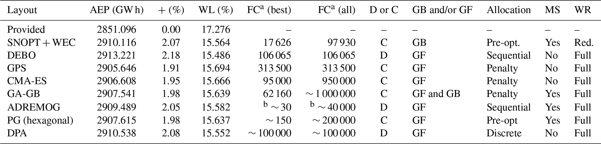
a Function calls are not directly comparable due to the use of a reduced wind rose, alternate implementations, surrogate models, etc. b Estimated equivalent function calls based on relative time required for the PAM surrogate model. Note: + signifies AEP increase from the provided layout, WL signifies wake loss, FC signifies function calls, C signifies continuous, D signifies discrete, GB signifies gradient-based, GF signifies gradient-free, pre-opt. signifies pre-optimization, MS signifies multi-start, WR signifies wind resource, and red. signifies reduced.
Some optimization method attributes are also provided in Table 2. Three of the methods used a discrete problem formulation, meaning that the potential wind turbine locations were limited to predetermined locations (though DEBO does adjust the resolution of the discretization during the optimization). The other five methods used continuous formulations, allowing wind turbines to be placed anywhere within the wind farm boundaries. Most of the methods are gradient-free algorithms. Only one, SNOPT + WEC, used a strictly gradient-based approach, and one, GA-GB, used a hybrid approach beginning with a gradient-free method and refining the resulting layout with the gradient-based SNOPT algorithm. Four types of allocation methods were used to assign turbines to boundary regions: (1) pre-optimization with only the outer boundaries, with turbines then being assigned to the nearest region; (2) sequential approaches where turbines were added to the initial layout according to various heuristics; (3) penalty approaches that slowly increased penalties for infeasible layouts during the optimization so turbines could move freely about the full wind farm space at the beginning; and (4) leveraging a discrete formulation so that turbines could move freely about the farm, even jumping between regions, throughout the optimization. To help avoid the problems of local optima, half of the algorithms used a multi-start approach. To reduce computational costs, one method (SNOPT + WEC) used a reduced wind rose with only a single wind speed in each of 100 wind directions, and one method (ADREMOG) used the PAM surrogate model.
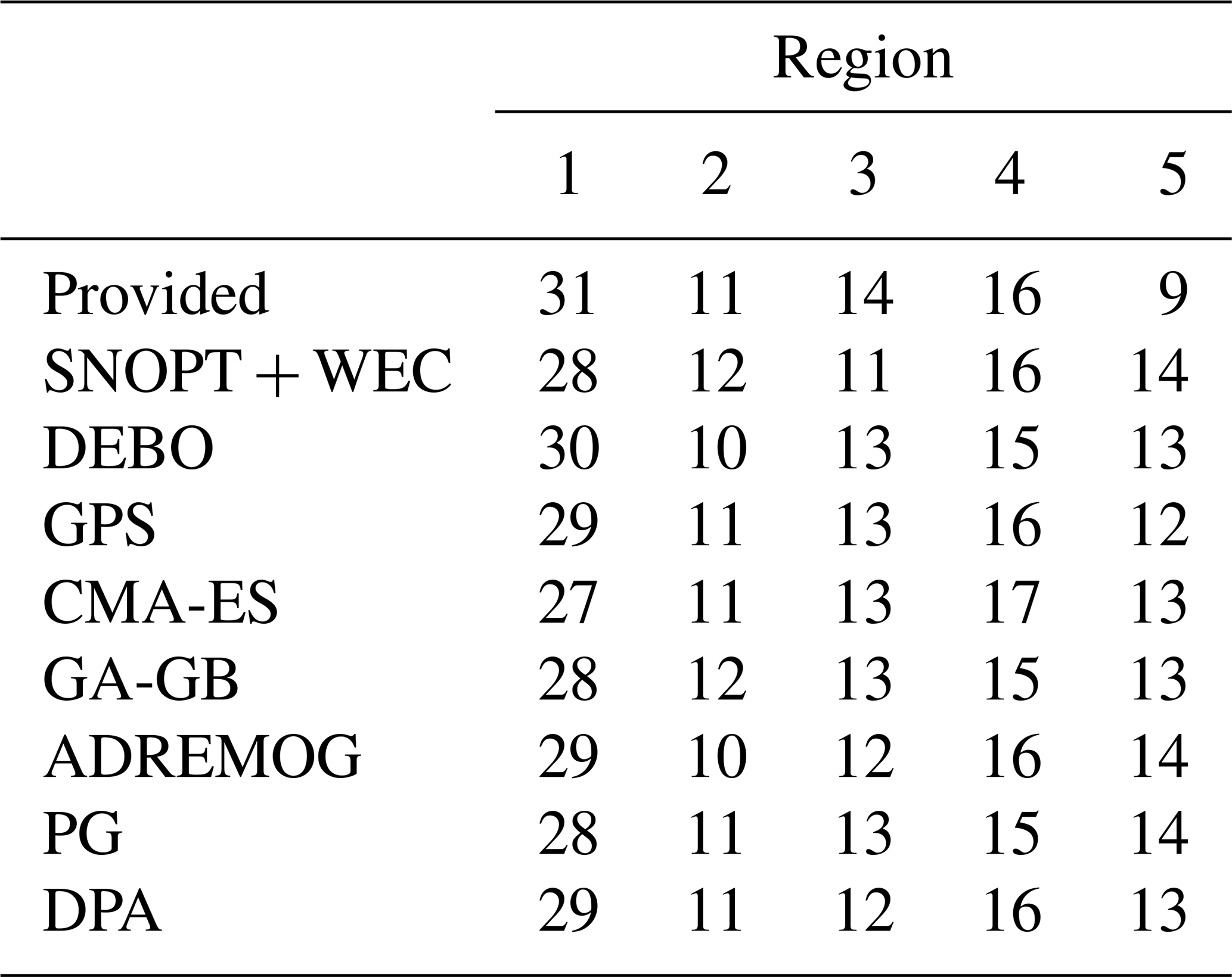
The optimized layouts found by each optimization method are shown in Fig. 10. All of the optimized layouts show similar characteristics. Most notably, all algorithms placed many turbines, with close spacing, along the outside boundaries of the wind farm where freestream wind is available. All the algorithms also provided a large space between the turbines on the boundary and the turbines placed on the inside areas. Turbines in the inner area are also much more spread out than the turbines on the edges. The number of turbines allocated by each optimization method to each region is shown in Table 3. All the optimization methods adjusted the number of turbines in at least some of the regions. All methods reduced the number of turbines in region 1 by at least one. The number of turbines in regions 2 and 4 were increased or decreased by one at the most. The number of turbines in region 3 was reduced by one to three by each method. The number of turbines in region 5 was increased by three to five by every optimization method. The methods all agreed on the number of turbines in each region to within three turbines for region 1 and within two turbines for regions 2 to 5. The following subsections present algorithm-specific results.
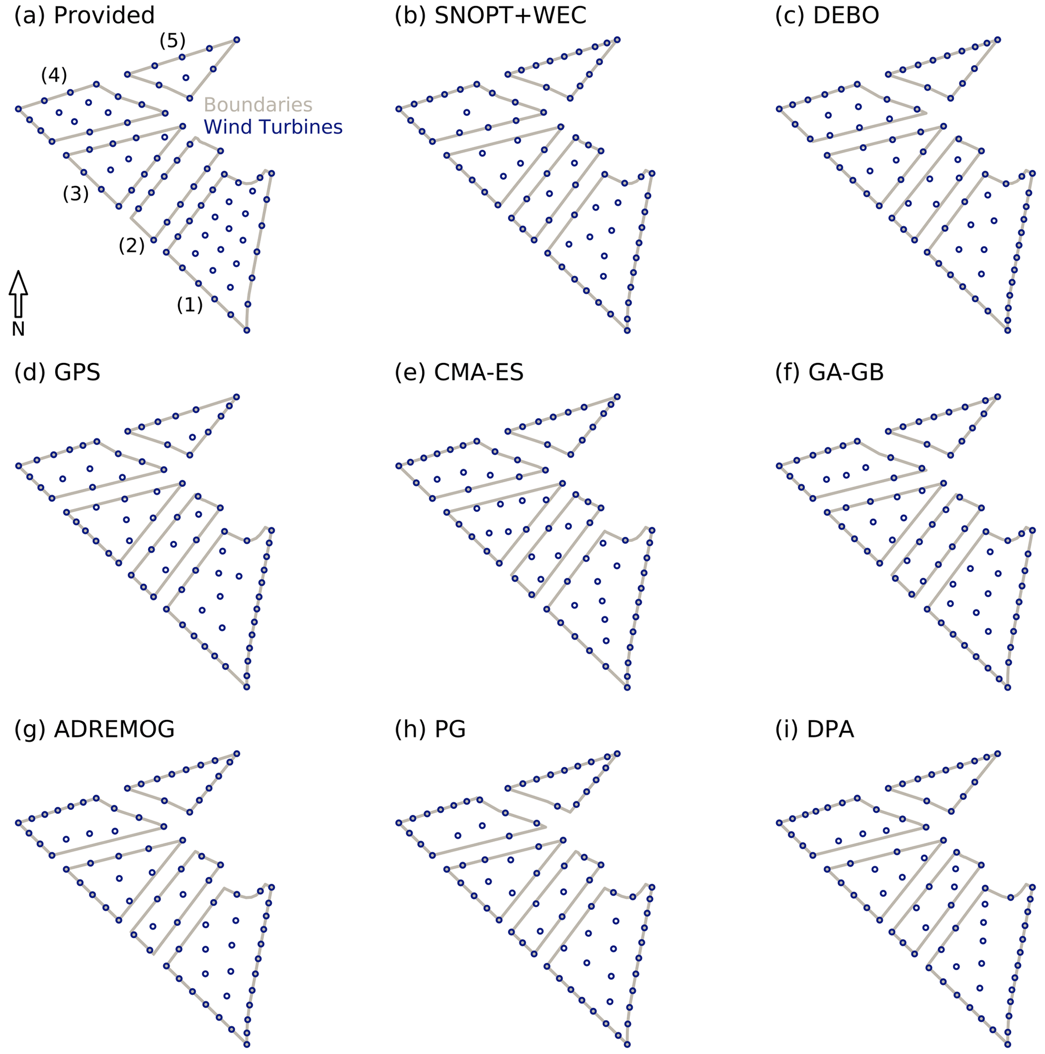
Table 3Turbine-to-region allocation for each algorithm's best layout. All layouts have a total of 81 turbines.
3.1 Sparse nonlinear optimizer with wake expansion continuation (SNOPT + WEC) results
We ran the SNOPT + WEC method with 10 different starting layouts (nine as described in Sect. 2.1 and one using the provided layout). We ran the optimizations using a single core on a MacBook Pro laptop with a 2 GHz Dual-Core Intel Core i5 processor. Run times ranged from 1.85 min to 31.33 min, with an average run time of 16.50 min. The AEP values for the SNOPT + WEC results ranged from 2898.841 to 2910.116 GW h with an average AEP of 2906.321 GW h. A total of 6 of the 10 optimized AEP values were in the range of the best layouts found by the other optimization algorithms. The best layout found by the SNOPT + WEC approach is shown in Fig. 10b.
While larger than many of the wind farm layout optimization problems presented in the literature, the problem presented here is still relatively small compared to many real-world problems. Because gradient-based methods scale well to problems with many variables and constraints, SNOPT + WEC would likely still perform well on larger problems without excessive computational cost.
3.2 Discrete exploration-based optimization (DEBO) results
The DEBO method found the best layout across all algorithms in terms of the objective function. The only layout found with DEBO is shown in Fig. 10c. While DEBO followed the same general trends as the other algorithms in turbine placement, it placed more turbines in region 1 than any of the other methods. DEBO was run in parallel using 10 Intel(R) Xeon(R) Gold 5120 2.20 GHz cores. Because there is little randomness associated with the DEBO algorithm, only one run was needed. The run took about 111 min.
3.3 Generalized pattern search (GPS) results
The best layout found by GPS is shown in Fig. 10d. While the initial layout does not change the distribution of turbines among the discrete regions compared to the baseline layout, the GPS solver moved a few turbines between regions during the optimization. Turbines in the center of the site experienced larger shifts, whereas turbines on the boundaries were not moved much from their initial positions. This confirms the initial expectation that perimeter-heavy layouts offer improved energy production.
The total improvements result from two separate steps in the GPS algorithm. First, the described adaptation of the initial layout reduces the total wake loss percentage to 16.386 % (approximately 56 % of the total reduction). The subsequent optimization with the GPS solver then yields the remaining 44 % of the wake loss reduction. The optimization included approximately 313 500 function calls and ran for approx. 6.2 h on a standard desktop PC. Most of the improvements in energy production were already achieved after half the time. Infeasible layouts result in a significant drop in the metric due to the applied energy yield penalty. The penalty magnitude depends on the number of invalid turbine locations.
3.4 Covariance matrix adaptation evolutionary strategy (CMA-ES) results
The AEP function used for optimization sampled the wind rose in 1∘ steps to avoid the artificial increase in AEP by aligning the wind turbines in wind directions not sampled. Wind speeds were sampled at every few meters per second from the Weibull distribution. The best layout found by CMA-ES is shown in Fig. 10e.
To assess the capability of the optimization algorithm alone and avoid influencing the search, a random infeasible initial layout is generated at every run. This initial layout packs turbines very closely together at the center of the site. The initial mean standard deviation of the search is small, so wind turbines begin moving slowly around their initial position. As the search evolves, the turbines move away from each other to minimize wake losses and find a good spatial distribution of turbines within the whole site, including locations outside the boundary of the whole site. Once convergence is achieved and an infeasible layout that maximizes AEP is found, inter-turbine spacing and corridor constraint penalties kick in, leading to turbines self-accommodating to find a feasible layout. Afterward, only feasible layouts are explored to maximize AEP again. The fitness function is equal to the AEP in the fourth stage, when all constraint penalties are zero. The results reported required approximately 5000 iterations. Each iteration evaluates 19 layouts; thus, the AEP function is called 95 000 times. Each optimization run takes approximately 1 h using 12 parallel threads at 3.2 GHz.
The layout was optimized 10 times, with the best wake loss ranging from 15.88 % to 15.67 %. The best layout found across 10 optimization runs places 49 turbines at the outer boundaries of the site and the remaining 32 turbines within (see Fig. 10e). The best locations found within the outer boundary seem to roughly fall into a grid. A quick analysis demonstrated that the wind turbines placed within 6 rotor diameters of other neighbors align with them at directions between 330 and 360∘, between 80 and 95∘, and between 37 and 60∘ wind directions, and no neighbors aligned in the 96 to 147∘ direction range. These directions are consistent with the highest-frequency wind directions in the wind rose, demonstrating that the method can find the most beneficial alignments for energy capture.
3.5 Genetic- and gradient-based hybrid algorithm (GA-GB) results
The AEP calculations used in the GA-GB optimizations were preformed with the full 1∘ resolution wind rose, using all the provided wind information. In reality, a coarser wind rose could be used to still achieve comparable results, but due to the relatively small computational burden, the full wind rose was used. We reduce the overall computational cost of this hybrid approach by only starting the gradient-based optimizations from the initial layouts with the highest AEP values. Using a laptop with a 2.6 GHz quad-core processor and 16 GB of ram, each iteration of the GA takes about 3 s, which results in the full GA run taking about 10 min. Each major iteration of SNOPT takes 1 to 2 min due to the finite-differencing required to obtain the gradient information of the model; we get a converged layout in about 1 h. About 2800 function calls were used in the GA placement algorithm, and approximately 25 000 function calls were used for each gradient-based optimization. Because there were 20 gradient-based optimizations performed, the total number of function calls for this study is approximately 500 000. Each gradient-based optimization took a different number of function calls due to them reaching the convergence criteria at different optimization iterations.
The best layout found with the GA-GB method is shown in Fig. 10f. The optimized turbine placement, although not regular, is generally feasible. There is some relatively close spacing along some of the boundaries of the wind energy areas, but with the availability of dedicated transit ways through the farm, this is not necessarily a concern for shipping traffic and transportation. Additionally, turbines are more spaced out along internal boundaries. Based on the NW–W–SW bias of the wind rose, direct lines of interior turbines that align with these directions are minimized, and when they do exist, the spacing between the turbines in these directions appears to be maximized while being balanced with neighboring edge turbines. This behavior follows results of other optimization algorithms.
3.6 Add–remove–move greedy (ADREMOG) results
The best layout found using ADREMOG is shown in Fig. 10g. ADREMOG has important trade-offs between the quality of the layouts and the time of execution. ADREMOG benefits from fine discretization. The median efficiency value of the layouts improves as the number of possible positions increases, as does the quality of the best-encountered layout. The best outcome corresponds to a wake loss efficiency of 15.582 %; the majority of the ADREMOG results fall within a range of 0.3 percentage points of the best outcome. Additionally, PAM overestimates power losses compared to the traditional AEP calculation approach. Nevertheless, the use of PAM does not compromise the ability of ADREMOG to build efficient layouts, as the correlation between the two assessment methods is strong.
Furthermore, this surrogate model allows us to avoid from 3 985 200 to 6 013 800 regular function calls that ADREMOG would have required to generate one layout for 8200 possible positions. The advantage is even more substantial, considering that a multi-start approach is necessary for identifying the best local minimum. The PAM needs to be generated only once for the whole process. Figure 11 presents the time demanded by the optimization procedure, to which it contributes the creation of the PAM and, after, the execution of ADREMOG for each initial position investigated. The data refer to a common PC with 16GB RAM running in serial.
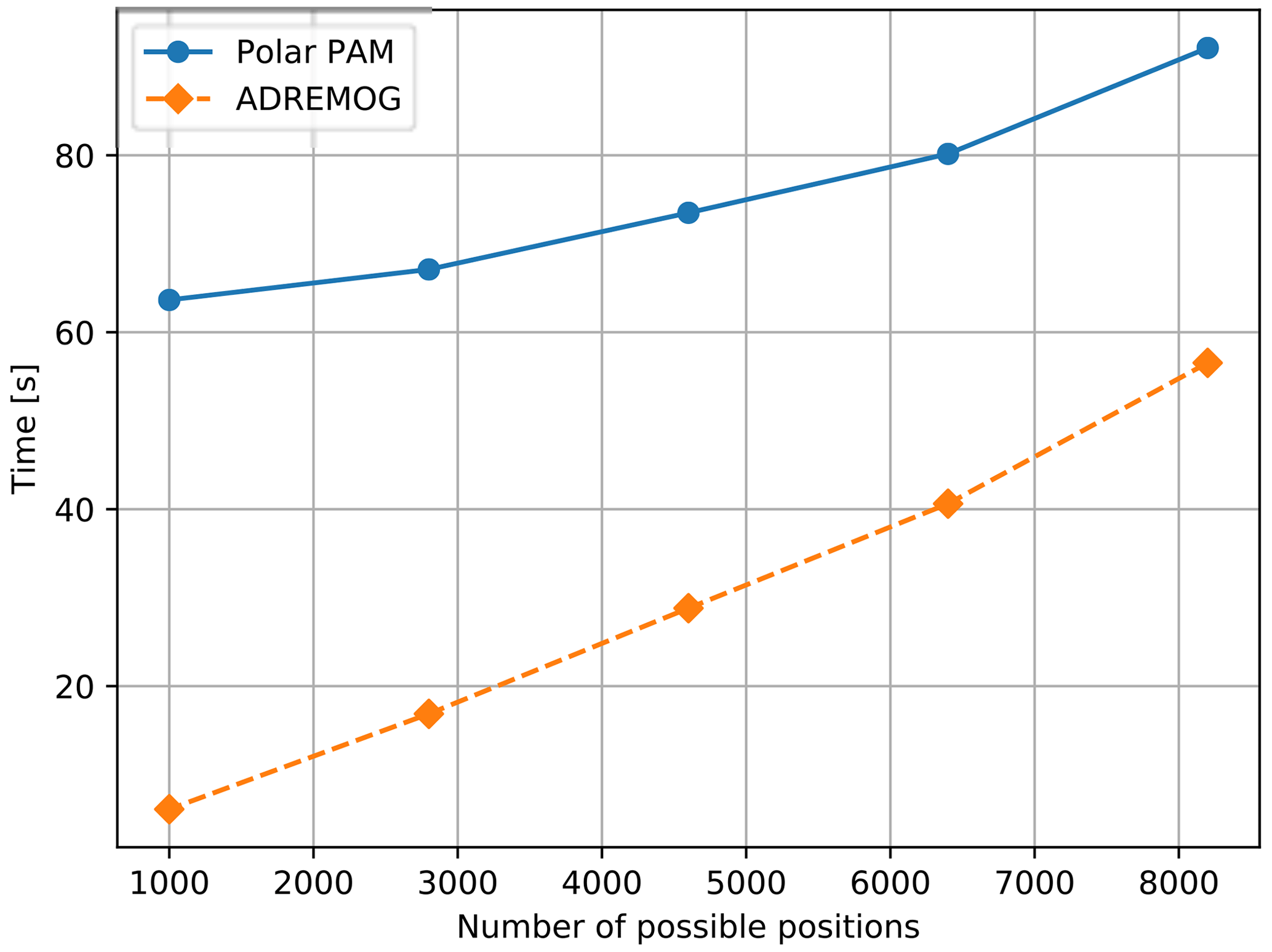
3.7 Pseudo-gradient optimization (PG) results
To test pseudo-gradient-based optimization, 1980 initial layouts were generated for both the hexagonal (random initial orientation) and ADREMOG (random position first turbine) approaches. Each of the initial layouts was then optimized with the same optimizer parameters. The best layout found by PG optimization starting from a hexagonal layout is shown in Fig. 10h.
Figure 12 shows the results for the hexagonal initial layouts as a scatter plot. On the horizontal (vertical) axis the wake loss percentage of the initial (optimized) layout is shown. Each layout is represented by a dot, the color of which indicates the number of pseudo-gradient (PG) iterations of the corresponding optimization run. Both initial and optimized wake loss percentages span about 0.8 percentage points, and the average improvement due to PG is about the same (cf. diagonal lines), albeit with a large variance. Nevertheless, because of the low computational cost of PG optimization (relative to most other approaches), it is reasonable to use it to slightly improve any layout, as was done in the analysis with the ADREMOG starts. For this problem, the magnitude of improvement achieved is significant. The number of iterations required for each optimization run is small, and most gains are made in the first 10 iterations. This means that the computational requirements are relatively light.
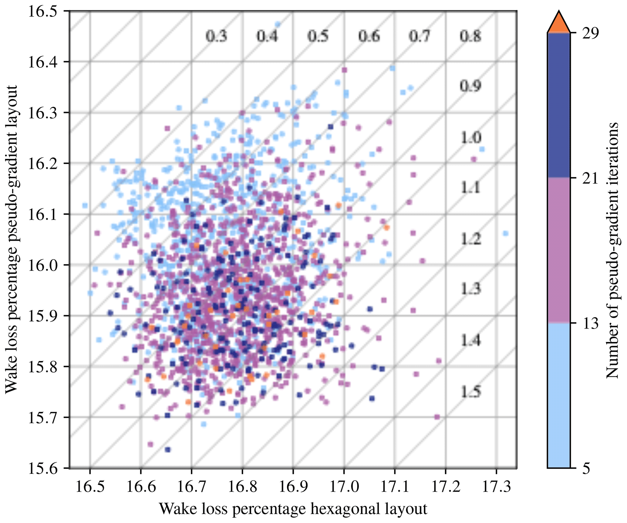
Figure 12Wake loss percentage of 1980 optimized layouts starting from random hexagonal layouts. Diagonal lines indicate the improvement due to PG.
It is interesting to note in Fig. 12 that the initial hexagonal layouts in general already provide improved performance over the provided layout. Roughly, an average improvement of 0.5 to 0.7 percentage points is obtained as compared to the manual layout provided. The hexagonal layout generation procedure can therefore be seen as a computationally very cheap random-search-type optimization algorithm that does not use any wake model calls.
Figure 13 shows the results for the ADREMOG-generated initial layouts as a scatter plot. On the horizontal axis the wake loss percentage of the optimized layout is shown. On the vertical axis, the wake loss percentage point improvement due to PG is given. Each layout is represented by a dot, the color of which indicates the number of ADREMOG iterations used to generate the initial layout. The number of PG iterations generally remained below 10. The wake loss percentages span almost 0.4 percentage points, but the improvement due to PG is small, up to 0.05 percentage points but typically around 0.01. So the PG-based algorithm manages to squeeze a little more efficiency out of the layouts, but the amount is not significant. There is no clear correlation between the number of ADREMOG iterations and the quality of the initial or optimized layouts.
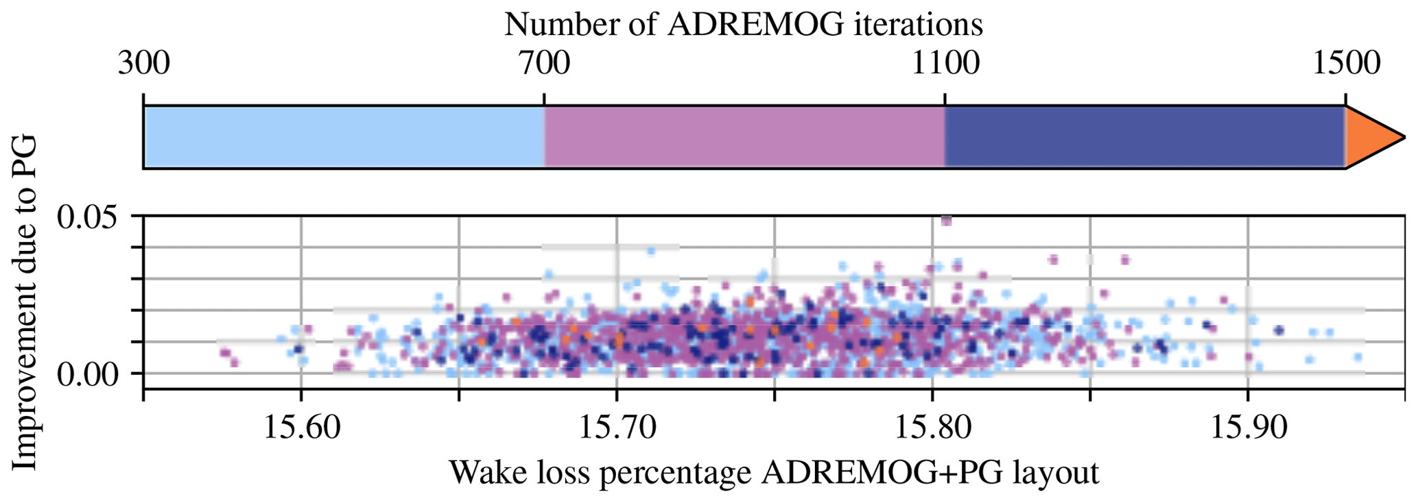
A general conclusion about the use of the PG optimizer is that while it can provide significant gains for non-optimized initial layouts (e.g., hexagonal grid starts), this is not the case for optimized ones (e.g., ADREMOG starts). Nevertheless, because of the low computational cost of PG optimization (relative to most other approaches), there is little reason to not use it to try and improve any layout slightly, as was done in the analysis with the ADREMOG starts.
3.8 Discrete perturbation algorithm (DPA) results
The DPA method found the second best layout across all algorithms in terms of the objective function. The layout found with DPA is shown in Fig. 10i. While DPA followed the same general trends as the other algorithms in turbine placement, it placed the same number of turbines in each region as the DEBO method, except for one less turbine in region 1 and one more turbine in region 4. DPA was run only once and ran on a 3.5 GHz AMD Ryzen 9 3950X processor using between 16 and 32 cores. DPA was allowed to run for 24 h.
The resulting layouts and related metrics indicate that all of the algorithms included in this study performed at a similar level in terms of layout quality. Similar to previous findings by Stanley and Ning (2019), placing most of the turbines on the boundary is advantageous for energy production, even if the turbine spacing is closer than the typical rules of thumb. The existence of shipping and infrastructure lanes through the farm should ensure that the close spacing on the outer boundaries does not impede maintenance and other necessary activities.
The highly multimodal nature of the wind farm layout optimization problem is very apparent in the results. Each optimization method found a different layout, but all were similar in performance according to the AEP and wake loss. However, though the total spread in optimized AEP of 7.575 GW h is small in terms of total electricity generation, it represents a potential annual revenue difference of over USD 1 million assuming a price per kilowatt-hour of USD 0.15 (Eurostat, 2021). Thus, for large farms like the one in this study, even small energy gains can make a significant financial difference. However, the simple wake models used for layout optimization do not have high enough accuracy to be certain of the differences between the layouts found in this study, so we cannot conclusively say which layout will be the best or what the true performance differences would be in actual practice.
The computational cost of each of the methods is difficult to compare due to factors such as different hardware, wind resource discretization, gradient computation, and surrogate modeling. We have included function call information for the best layout found by each algorithm and the total number of function calls used across all runs. This information is helpful in assessing relative computational cost but should be used carefully. The PAM surrogate model significantly reduced the time required to optimize, but the ADREMOG approach required many multi-starts to find its best layout. Other methods also rely on some number of multi-starts to overcome the multimodality of the problem. Using a multi-start approach substantially increases the computational cost, but total cost may still be less for multi-start approaches than others if the algorithm itself is cheap enough. We found that multi-start approaches were not necessarily more costly than ones using a single run, and multi-start approaches represent half of the top four layouts by AEP.
The use of a discrete or continuous design space formulation can significantly impact the results. Although a discrete formulation limits which turbine locations are available, the two best layouts (DEBO and DPA) were found using discrete problem formulations. This indicates that the limitation on potential turbine locations does not necessarily preclude such methods from finding optimal layouts. Continuous formulations provide more options but suffer from having potentially too many options to explore effectively.
Because only one method was purely gradient-based, it is hard to draw many conclusions about the trade-offs between gradient-free and gradient-based algorithms. The gradient-based method, SNOPT + WEC, ranked third overall in terms of AEP and wake loss. SNOPT + WEC used relatively fewer function calls and had low CPU time. This seems to indicate that at least this gradient-based method can achieve comparable results in less time than many gradient-free methods on the wind farm layout optimization problem. More work could still be done to reduce the computational cost and further improve exploration.
Few clear trends were shown between turbine-to-region allocation and layout quality. Three of the four allocation method types showed up in the top four layouts. However, because all methods moved turbines between regions, especially adding many turbines to region 5, we can say that allocating the right number of turbines to each discrete region in the farm is critical to finding the best layouts. Optimization methods that used penalty methods for turbine-to-region allocation did not perform as well as those using the other allocation methods. The best layout by AEP was found using a sequential allocation method.
While it is important to weigh the quality of results and computational cost of each algorithm, the developer cost and level of expertise are also important to balance. Off-the-shelf algorithms, such as GPS and CMA-ES, may be well documented but may not perform as well as newer methods not yet available in standard code packages. Commercial code implementations, such as SNOPT and GPS, require a license, but they are well documented. Open-source-only methods may take a little more effort to run but may also have more recent algorithm developments. Newly developed algorithms, such as DEBO, WEC, ADREMOG, and PG, may be available through research codes or may need to be reimplemented. Implementations of industry methods like DPA may not be available but could be approximated, which may require substantial effort for development and fine-tuning. Also important to consider are the additional efforts involved for various peripherals such as discretizing the design space, altering the wake model to accommodate algorithmic differentiation or WEC, obtaining gradients, preparing and running a multi-start optimization, reducing the wind resource, defining initial layouts, or setting up a turbine-to-region allocation method. When selecting which algorithm to use, carefully weigh the requirements and available resources in order to select the most suitable algorithm for the given situation.
While Herbert-Acero et al. (2014) refer to the no-free-lunch theorem as “for all possible performance measures, no algorithm is better than another when its performance is averaged over all possible optimization problems” (see Wolpert and Macready, 1997, for more details on no-free-lunch theorems), Herbert-Acero et al. (2014) also point out that individual algorithms may be effectively tuned to perform well on specific optimization problems. In this work we found that none of the algorithms significantly outperformed the others and attribute this similar performance, in part, to the tuning of each algorithm to this problem by individual experts, which is one of the key differences between this and most of the previous comparative studies of optimization algorithms applied to wind farm layout optimization problems. The similarity may also be partly due to the problem being somewhat flat with many similar local optima. However, the DEBO algorithm was developed specifically for this case study, and it did find the layout with the highest AEP. It will be interesting to see how the DEBO method performs in future comparisons and other problems.
In this work we introduced eight optimization methods (including one new algorithm), applied them to the IEA case study 4 (with 81 turbines and 5 discrete boundary regions, including some concavities), and presented and discussed the results. We found that all eight algorithms performed well, both gradient-based and gradient-free, with optimized wake loss values between 15.48 % and 15.70 %. One of the key differences between this and previous studies is that each optimization method was managed by experts in that method. Thus, user error is less likely to have impacted the results. Having specialists in each method manage the optimizations likely contributed significantly to the fairly even performance of the various methods.
The most obvious similarity between the layouts found by all the optimization methods tested is that turbines were packed closely on the outer boundaries and much more spread out in the internal areas of the wind farm. All the methods placed similar numbers of turbines in each region, but methods that used penalty functions for constraints and turbine-to-region allocation resulted in lower optimized AEP values. The best layout in terms of wake loss was found using discrete exploration-based optimization (DEBO), a gradient-free method using a discrete problem formulation that was developed specifically for this case study. However, we also found that continuous formulations can also be effective.
While we believe the optimization method comparisons presented herein will be useful to the community, they are not perfect. It is important that more comparisons of algorithms on wind farm layout optimization problems be performed to better assess the performance trade-offs of the various algorithms and peripheral methods. Future studies will likely benefit from the collaborative model used here, enlisting experts in the various algorithms so that each algorithm is less likely to be negatively influenced by user error. However, carefully creating and following clear protocols for gathering and reporting information about the optimizations is critical, particularly when working with many researchers. Future comparisons should run all optimization methods on the same hardware and establish uniform criteria for estimating computation costs in terms of time and function evaluations. The standardized ontologies being created by the IEA Wind Task 37 (Dykes et al., 2017) will likely help significantly with performing future comparative studies of wind farm layout optimization methods.
Layout files, the provided physics model, some figure and table generation scripts, and other data are available at https://github.com/jaredthomas68/thomas2022-8-opt-algs-wflop (last access: 11 May 2023) or https://doi.org/10.5281/zenodo.7125349 (Thomas, 2022a).
The Julia implementation of the wake and farm model used for the SNOPT + WEC method (see Sects. 2.1 and 3.1) is available in FLOWFarm.jl at https://github.com/byuflowlab/FLOWFarm.jl/tree/develop (last access: 11 May 2023) at commit “ec5270203786d5bcf065fff8c80bd7710906a40e” and preserved with a DOI at https://doi.org/10.5281/zenodo.7125827 (Thomas et al., 2022b).
The code for pseudo-gradient-based optimization (see Sects. 2.7 and 3.7) is publicly available (Quaeghebeur, 2020) (https://doi.org/10.5281/zenodo.4072253). It also includes functionality for generating a pre-averaged model (see Sects. 2.6 and 3.6) and using a form of wake expansion (e.g., Sect. 2.1; called “wake spreading” in the code; not reported on in this paper).
JJT managed the collaborative efforts of the paper, led the combined analysis of the results, directed the use of one optimization method, and edited the full manuscript. He also wrote some of the algorithm-specific sections and all of the non-algorithm-specific sections of the paper. NFB led the case study preparation and wrote the related code and other documents, initiated collaborative work, and started the writing process. PM developed the DEBO algorithm specifically for this work, performed the DEBO optimization, and wrote the DEBO-specific sections. EQ revised the case study wind resource for this paper, performed optimizations for one algorithm and wrote the related algorithm-specific sections, supervised and supported FT, and contributed to the combined results analysis. SeS performed optimizations for one algorithm, wrote the related algorithm-specific sections, and contributed to the combined results analysis. JJ collaborated in performing optimizations for one algorithm and writing the related algorithm-specific sections. CB collaborated in performing optimizations for one algorithm and writing the related algorithm-specific sections. FT performed optimizations for one algorithm and wrote the related algorithm-specific sections. DB performed optimizations for one algorithm and wrote the related algorithm-specific sections. NR performed optimizations for one algorithm and wrote the related algorithm-specific methods section. APJS assisted in case study preparation, code development, and writing. WH performed optimizations and assisted in code development for one algorithm and assisted in writing the related algorithm-specific sections. WH also contributed to results synthesis and writing. AN acted as the principal investigator, providing direction, ideas, and feedback throughout the development of this work. All authors contributed conceptually to this work.
The contact author has declared that none of the authors has any competing interests.
Publisher’s note: Copernicus Publications remains neutral with regard to jurisdictional claims in published maps and institutional affiliations.
The authors would like acknowledge the valuable input of Katherine Dykes in the preparation of this work.
This work was authored in part by the National Renewable Energy Laboratory, operated by Alliance for Sustainable Energy, LLC, for the U.S. Department of Energy (DOE) under contract no. DE-AC36-08GO28308. Funding was provided by U.S. Department of Energy Office of Energy Efficiency and Renewable Energy Wind Energy Technologies Office. The views expressed in the article do not necessarily represent the views of the DOE or the U.S. Government. The U.S. Government retains and the publisher, by accepting the article for publication, acknowledges that the U.S. Government retains a nonexclusive, paid-up, irrevocable, worldwide license to publish or reproduce the published form of this work, or allow others to do so, for U.S. Government purposes.
A portion of the research was performed using computational resources sponsored by the U.S. Department of Energy Office of Energy Efficiency and Renewable Energy and located at the National Renewable Energy Laboratory.
A portion of the research was performed using computational resources managed by the Office of Research Computing at Brigham Young University.
Erik Quaeghebeur's contribution was part of the Dutch EUROS program, supported by the NWO domain Applied and Engineering Sciences and partly funded by the Dutch Ministry of Economic Affairs (grant no. 14187).
This research has been supported by the National Renewable Energy Laboratory (grant no. DE-AC36-08GO28308) and the Ministerie van Economische Zaken (grant no. 14187).
This paper was edited by Jonathan Whale and reviewed by two anonymous referees.
Arnoud, A., Guvenen, F., and Kleineberg, T.: Benchmarking Global Optimizers, Working Paper 26340, National Bureau of Economic Research, https://doi.org/10.3386/w26340, 2019. a
Baker, N. F., Stanley, A. P. J., Thomas, J. J., Ning, A., and Dykes, K.: Best Practices for Wake Model and Optimization Algorithm Selection in Wind Farm Layout Optimization, in: AIAA Scitech 2019 Forum, San Diego, CA, https://doi.org/10.2514/6.2019-0540, 2019. a, b, c, d, e
Baker, N. F., Thomas, J. J., Stanley, A. P. J., and Ning, A.: IEA Task 37 Wind Farm Layout Optimization Case Studies, Zenodo [code and data set], https://doi.org/10.5281/zenodo.5809681, 2021. a, b, c, d
Bastankhah, M. and Porté-Agel, F.: Experimental and theoretical study of wind turbine wakes in yawed conditions, J. Fluid Mech., 806, 506–541, https://doi.org/10.1017/jfm.2016.595, 2016. a
Belegundu, A. D. and Chandrupatla, T. R.: Optimization Concepts and Applications in Engineering, 2nd Edn., Cambridge University Press, ISBN 13:978-0521878463, 2011. a
Bezanson, J., Edelman, A., Karpinski, S., and Shah, V. B.: Julia: A fresh approach to numerical computing, SIAM Rev., 59, 65–98, https://doi.org/10.1137/141000671, 2017. a
Bortolotti, P., Dykes, K., Merz, K., Sethuraman, L., and Zahle, F.: IEA Wind Task 37 on System Engineering in Wind Energy, WP2 – Reference Wind Turbines, Tech. rep., National Renewable Energy Laboratory (NREL), Golden, CO, USA, https://doi.org/10.2172/1529216, 2018. a
Brogna, R., Feng, J., Sørensen, J. N., Shen, W. Z., and Porté-Agel, F.: A new wake model and comparison of eight algorithms for layout optimization of wind farms in complex terrain, Appl. Energ., 259, 114189, https://doi.org/10.1016/j.apenergy.2019.114189, 2020. a, b, c, d, e
Dykes, K. L., Zahle, F., Merz, K., McWilliam, M., and Bortolotti, P.: IEA Wind Task 37: Systems Modeling Framework and Ontology for Wind Turbines and Plants, https://www.osti.gov/biblio/1375625 (last access: 29 May 2023), 2017. a
Eurostat: Electricity prices by type of user, Eurostat [data set], https://ec.europa.eu/eurostat/databrowser/view/ten00117/default/table?lang=en (last access: 29 May 2023), 2021. a
Feng, J. and Shen, W. Z.: Solving the wind farm layout optimization problem using random search algorithm, Renew. Energ., 78, 182–192, https://doi.org/10.1016/j.renene.2015.01.005, 2015. a, b, c
Fischetti, M. and Monaci, M.: Proximity search heuristics for wind farm optimal layout, J. Heuristics, 22, 459–474, 2016. a, b, c
Fleming, P., Ning, A., Gebraad, P., and Dykes, K.: Wind Plant System Engineering through Optimization of Layout and Yaw Control, Wind Energy, 19, 329–344, https://doi.org/10.1002/we.1836, 2015. a
Gebraad, P., Thomas, J. J., Ning, A., Fleming, P., and Dykes, K.: Maximization of the Annual Energy Production of Wind Power Plants by Optimization of Layout and Yaw-Based Wake Control, Wind Energy, 20, 97–107, https://doi.org/10.1002/we.1993, 2017. a
Gill, P., Murray, W., and Saudners, M.: SNOPT: an SQP algorithm for large-scale constrained optimization, SIAM Rev., 47, 99–131, 2005. a
Gill, P. E., Murray, W., and Saunders, M. A.: SNOPT: An SQP algorithm for large-scale constrained optimization, SIAM Journal of Optimization, 12, 979–1006, https://doi.org/10.1137/S1052623499350013, 2002. a
Grady, S., Hussaini, M., and Abdullah, M.: Placement of wind turbines using genetic algorithms, Renew. Energ, 30, 259–270, https://doi.org/10.1016/j.renene.2004.05.007, 2005. a, b
Gray, J. S., Hearn, T. A., Moore, K. T., Hwang, J., Martins, J., and Ning, A.: Automatic Evaluation of Multidisciplinary Derivatives Using a Graph-Based Problem Formulation in OpenMDAO, in: 15th AIAA/ISSMO Multidisciplinary Analysis and Optimization Conference, 16–20 June 2014, Atlanta, GA, https://doi.org/10.2514/6.2014-2042, 2014. a
Gray, J. S., Hwang, J. T., Martins, J. R. R. A., Moore, K. T., and Naylor, B. A.: OpenMDAO: An Open-Source Framework for Multidisciplinary Design, Analysis, and Optimization, Struct. Multidiscip. O., 59, 1075–1104, https://doi.org/10.1007/s00158-019-02211-z, 2019. a
Griewank, A. and Walther, A.: Evaluating Derivatives: Principles and Techniques of Algorithmic Differentiation, Society for Industrial and Applied Mathematics, 2nd Edn., ISBN 978-0-89871-659-7, eISBN 978-0-89871-776-1, https://doi.org/10.1137/1.9780898717761, 2008. a
Guirguis, D., Romero, D. A., and Amon, C. H.: Toward efficient optimization of wind farm layouts: Utilizing exact gradient information, Appl. Energ., 179, 110–123, https://doi.org/10.1016/j.apenergy.2016.06.101, 2016. a, b, c, d, e, f
Ha, D.: A Visual Guide to Evolution Strategies, blog.otoro.net, https://blog.otoro.net/2017/10/29/visual-evolution-strategies/ (last access: 29 May 2023), 2017. a
Hansen, N., Akimoto, Y., and Baudis, P.: CMA-ES/pycma on Github, Zenodo [code], https://doi.org/10.5281/zenodo.2559634, 2019. a
Herbert-Acero, J., Probst, O., Rethore, P., Larsen, G., and Castillo-Villar, K.: A Review of Methodological Approaches for the Design and Optimization of Wind Farms, Energies, 7, 6930–7016, https://doi.org/10.3390/en7116930, 2014. a, b, c, d
IEA: IEA Wind Task 37, https://iea-wind.org/task37/ (last access: 29 May 2023), 2021. a
Katic, I., Højstrup, J., and Jensen, N.: A Simple Model for Cluster Efficiency, in: European Wind Energy Association Conference and Exhibition, European Wind Energy Association, Rome–Italy, 1986. a
Koziel, S. and Yang, X.-S. (Eds.): Computational Optimization, Methods and Algorithms, Studies in Computational Intelligence, Springer, Berlin, Heidelberg, ISBN 978-3-642-20858-4, https://doi.org/10.1007/978-3-642-20859-1, 2011. a
Kunakote, T., Sabangban, N., Kumar, S., Tejani, G. G., Panagant, N., Pholdee, N., Bureerat, S., and Yildiz, A. R.: Comparative Performance of Twelve Metaheuristics for Wind Farm Layout Optimisation, Arch. Comput. Meth. E., 29, 717–730, https://doi.org/10.1007/s11831-021-09586-7, 2022. a, b, c
Lambe, A. B. and Martins, J. R. R. A.: Extensions to the Design Structure Matrix for the Description of Multidisciplinary Design, Analysis, and Optimization Processes, Struct. Multid. O., 46, 273–284, https://doi.org/10.1007/s00158-012-0763-y, 2012. a
Martins, J. R. R. A. and Hwang, J. T.: Review and Unification of Methods for Computing Derivatives of Multidisciplinary Computational Models, AIAA J., 51, 2582–2599, https://doi.org/10.2514/1.J052184, 2013. a
Martins, J. R. R. A. and Ning, A.: Engineering Design Optimization, Cambridge University Press, https://doi.org/10.1017/9781108980647, 2021. a
MathWorks: MATLAB Direct search function, https://de.mathworks.com/help/gads/patternsearch.html (last access: 3 July 2020), 2020. a
Mobahi, H. and Fisher III, J.: A Theoretical Analysis of Optimization by Gaussian Continuation, in: Vol. 29, Proceedings of the AAAI Conference on Artificial Intelligence, https://doi.org/10.1609/aaai.v29i1.9356, 2015. a, b
Mosetti, G., Poloni, C., and Diviacco, B.: Optimization of wind turbine positioning in large windfarms by means of a genetic algorithm, J. Wind Eng. Ind. Aerod., 51, 105–116, https://doi.org/10.1016/0167-6105(94)90080-9, 1994. a
Niayifar, A. and Porté-Agel, F.: Analytical Modeling of Wind Farms: A New Approach for Power Prediction, Energies, 9, 741, https://doi.org/10.3390/en9090741, 2016. a
Ning, A.: Sparse Nonlinear Optimization Wrapper (SNOW), GitHub [code], https://github.com/byuflowlab/SNOW.jl (last access: 29 May 2023), 2021. a
Press, W. H., Teukolsky, S. A., Vetterling, W. T., and Flannery, B. P.: Numerical Recipes: The Art of Scientific Computing, 3rd Edn., Cambridge University Press, ISBN 13:978-0521880688, 2007. a, b
Quaeghebeur, E.: equaeghe/wflopg: Initial release, Zenodo [code], https://doi.org/10.5281/zenodo.4072253, 2020. a
Quaeghebeur, E., Bos, R., and Zaaijer, M. B.: Wind farm layout optimization using pseudo-gradients, Wind Energ. Sci., 6, 815–839, https://doi.org/10.5194/wes-6-815-2021, 2021. a, b, c
Réthoré, P.-E., Fuglsang, P., Larsen, G. C., Buhl, T., Larsen, T. J., and Aagaard Madsen, H.: TOPFARM: Multi-fidelity optimization of wind farms, Wind Energy, 17, 1797–1816, 2014. a
Revels, J., Lubin, M., and Papamarkou, T.: Forward-Mode Automatic Differentiation in Julia, arXiv [preprint], https://doi.org/10.48550/arXiv.1607.07892, 2016. a
Rios, L. M. and Sahinidis, N. V.: Derivative-free optimization: a review of algorithms and comparison of software implementations, J. Global Optim., 56, 1247–1293, https://doi.org/10.1007/s10898-012-9951-y, 2013. a
Serrano González, J., Trigo García, Á. L., Burgos Payán, M., Riquelme Santos, J., and González Rodríguez, Á. G.: Optimal wind-turbine micro-siting of offshore wind farms: A grid-like layout approach, Appl. Energ., 200, 28–38, https://doi.org/10.1016/j.apenergy.2017.05.071, 2017. a
Stanley, A. P. J. and Ning, A.: Massive simplification of the wind farm layout optimization problem, Wind Energ. Sci., 4, 663–676, https://doi.org/10.5194/wes-4-663-2019, 2019. a, b, c, d
Thomas, J.: jaredthomas68/thomas2022-8-opt-algs-wflop: Initial release (submission), Zenodo [code and data set], https://doi.org/10.5281/zenodo.7125349, 2022a. a
Thomas, J., Gebraad, P., and Ning, A.: Improving the FLORIS Wind Plant Model for Compatibility with Gradient-Based Optimization, Wind Engineering41, 313–329, https://doi.org/10.1177/0309524X17722000, 2017. a
Thomas, J. J. and Ning, A.: A Method for Reducing Multi-Modality in the Wind Farm Layout Optimization Problem, J. Phys.-Conf. Ser., 1037, 042012, https://doi.org/10.1088/1742-6596/1037/4/042012, 2018. a
Thomas, J. J., Annoni, J., Fleming, P., and Ning, A.: Comparison of Wind Farm Layout Optimization Results Using a Simple Wake Model and Gradient-Based Optimization to Large-Eddy Simulations, in: AIAA Scitech 2019 Forum, 7–11 January 2019, San Diego, California, https://doi.org/10.2514/6.2019-0538, 2019. a
Thomas, J. J., McOmber, S., and Ning, A.: Wake Expansion Continuation: Multi-Modality Reduction in the Wind Farm Layout Optimization Problem, Wind Energy, 25, 678–699, https://doi.org/10.1002/we.2692, 2022a. a, b, c, d, e
Thomas, J., Stanley, P. J., Lee, E., Holt, W., Baker, N. F., and Ning, A.: jaredthomas68/FLOWFarm.jl: For 8 algorithms WFLOP paper (thomas2022-8-algs-wflop), Zenodo [code], https://doi.org/10.5281/zenodo.7125827, 2022b. a
Tilli, F.: Greedy wind farm layout optimization using pre-averaged losses, Master's thesis, Delft University of Technology, http://resolver.tudelft.nl/uuid:4b118ae1-536d-4e0b-a30b-d88ba818c918 (last access: 11 May 2023), 2019. a
Turner, S., Romero, D., Zhang, P., Amon, C., and Chan, T.: A new mathematical programming approach to optimize wind farm layouts, Renew. Energ., 63, 674–680, https://doi.org/10.1016/j.renene.2013.10.023, 2014. a, b
Wasan, M. T.: Stochastic Approximation, in: Cambridge Tracts in Mathematics, Series Number 58, Cambridge University Press, ISBN 13:9780521073684, ISBN 10:0521073685, 1969. a
Wolpert, D. and Macready, W.: No free lunch theorems for optimization, IEEE T. Evolut. Comput., 1, 67–82, https://doi.org/10.1109/4235.585893, 1997. a
Wu, N., Kenway, G., Mader, C. A., Jasa, J., and Martins, J. R.: pyOptSparse: A Python framework for large-scale constrained nonlinear optimization of sparse systems, Journal of Open Source Software, 5, 2564, https://doi.org/10.21105/joss.02564, 2020. a
Yang, Q., Li, H., Li, T., and Zhou, X.: Wind farm layout optimization for levelized cost of energy minimization with combined analytical wake model and hybrid optimization strategy, Energ. Convers. Manageme., 248, 114778, https://doi.org/10.1016/j.enconman.2021.114778, 2021. a
Zergane, S., Smaili, A., and Masson, C.: Optimization of wind turbine placement in a wind farm using a new pseudo-random number generation method, Renew. Energ, 125, 166–171, https://doi.org/10.1016/j.renene.2018.02.082, 2018. a
The stochastic gradient mentioned here is not the same as the stochastic gradient used in the context of deep learning, although these methods do have the same name.