Investigation of blade flexibility effects on the loads and wake of a 15 MW wind turbine using a flexible actuator line method

This paper investigates the impact of blade flexibility on the aerodynamics and wake of large offshore turbines using a flexible actuator line method (ALM) coupled to the structural solver BeamDyn in large-eddy simulations. The study considers the IEA 15 MW reference wind turbine in close-to-rated operating conditions. The flexible ALM is first compared to OpenFAST simulations and is shown to consistently predict the rotor aerodynamics and the blade structural dynamics. However, the effect of blade flexibility on the loads is more pronounced when predicted using the ALM compared with using the blade element momentum theory. The wind turbine is then simulated in a neutral turbulent atmospheric boundary layer with flexible and rigid blades. The significant flapwise and torsional mean displacements lead to an overall decrease of 14 % in thrust and 10 % in power compared to a rotor with no deformation. These changes influence the wake through a reduced time-averaged velocity deficit and turbulent kinetic energy. The unsteady loads induced by the rotation in the sheared wind and the turbulent velocity fluctuations are also substantially affected by the flexibility and exhibit a noticeably different spectrum. However, the influence of these load variations on the wake is limited, and the assumption of rigid blades in their deformed geometry is shown to be sufficient to capture the wake dynamics. The influence of the resolution of the flow solver is also evaluated, and the results are shown to remain consistent between different spatial resolutions. Overall, the structural deformations have a substantial impact on the turbine performance, loads, and wake, which emphasizes the importance of considering the flexibility of the blades in simulations of large offshore wind turbines.

1 Introduction

Over the past few years, offshore wind energy has grown massively thanks to a drastic decrease in its levellized cost of energy. This significant reduction is primarily attributed to the increase in the rotor size, which tends to drive down both capital and operational expenditures. In fact, larger modern turbines typically exhibit a lower turbine cost per megawatt compared to their smaller counterparts. At the level of the wind farm, the decreased number of turbines also allows for reducing the cable requirements (Fingersh et al., 2006). The cost of maintenance per megawatt has also been reported to be a few percent lower per additional megawatt of rated power (Sørensen and Larsen, 2021). Furthermore, larger turbines typically have higher hub heights, which results in a more significant mean flow velocity across the rotor and hence an increased power extraction per unit area (Sørensen and Larsen, 2023). As a result, turbines with a rated power of 10–12 MW are now commonly used in offshore conditions, and the industry is rapidly developing 15–18 MW prototypes with blades much longer than 100 m.

However, as the rotor diameter increases, fundamental changes in design are necessary to constrain the total mass of the blades in order to reduce the centrifugal and gravitational loads acting upon them (Sieros et al., 2012). Therefore, recent blades are slender and made of lightweight composite materials, increasing their flexibility and potentially causing significant aeroelastic effects. The structural deformation of the blades modifies their aerodynamics by adding bending and twist, which can lead to substantial changes in the mean loads acting on the turbine. Additionally, the wind shear and turbulence create unsteady aeroelastic effects that impact the turbine lifetime. These variations can ultimately affect the flow past the turbine, modifying the wake evolution and recovery. A deeper understanding of the loads and wake of these large turbines is required to design reliable products and predict their interaction in a wind farm, which will allow for further reducing the cost of offshore wind energy.

The structural aspect is often neglected in simulations that use actuator line or disc methods to represent the flow past a turbine. While this approach was mostly valid for smaller turbines, the flow past large rotors is now noticeably affected by the changes in the aerodynamics. To evaluate these effects, some studies have considered the coupling of a flow solver to a structural solver using actuator methods as an interface. Storey et al. (2013) coupled OpenFAST to an actuator disc method to perform simulations of one or two turbines and to compare their results to measurements. Vitsas and Meyers (2016) used a modal structural model coupled to an actuator sector method to study two wind farm configurations. More recently, OpenFAST was also coupled to Nalu-Wind and PALM (Sprague et al., 2020; Krüger et al., 2022) to study the NREL 5 MW reference wind turbine. Hodgson et al. (2021) also performed validation of flexible actuator methods against high-fidelity blade-resolved simulations, highlighting the ability of the actuator line method (ALM) to accurately capture aeroelastic effects on rotors up to 5 MW (see also Sørensen et al., 2015; Hodgson et al., 2022). An elastic ALM based on the coupling between an ALM and an Euler beam model discretized using finite differences was also developed by Meng et al. (2018, 2020) and used for a pair of NREL 5 MW turbines and a wind farm. Spyropoulos et al. (2021) also developed a fluid–structure interaction framework based on the ALM in a flow solver for the compressible URANS equations. This framework uses a multi-body formulation with Timoshenko beam elements to solve the structural dynamics. It was compared in uniform flow against the blade element momentum (BEM) theory and a lifting line and was shown to accurately predict the blade deflections and the loads, also in yawed conditions. Della Posta et al. (2022, 2023) also considered a two-way coupling between a structural solver and an ALM, including the tower, for unsteady aerodynamics of the NREL 5 MW rotor. However, most of the aforementioned studies consider medium-scale rotors with simpler structural parameters than the new-generation turbines. Consequently, the effects of the nonlinearities induced by the large displacements are not considered. Additionally, the impact of the flexibility is rarely assessed by comparing the results to those obtained for rigid blades. Finally, most of the studies focus on the blade and rotor loads but do not assess the effect of the flexibility on the wake in depth.

This study investigates the effects of the deformation of the rotor on a very large reference wind turbine in realistic operating conditions. The open-source IEA 15 MW (Gaertner et al., 2020) turbine model is selected for its large rated power that is representative of modern large-scale offshore turbines and for its comprehensive documentation. Large-eddy simulations of the atmospheric boundary layer and the wake of the turbine are carried out using a flexible ALM coupled to the nonlinear structural solver BeamDyn from OpenFAST. Comparison between fully coupled aeroelastic simulations and simulations assuming rigid blades aims to provide a deeper understanding of the variation in the loads induced by the flexibility. Then, the effect of the blade displacement and load variation on the wake is assessed. The contribution of this study is therefore to provide further insights into the effect of the mean and unsteady deformations on the loads of the 15 MW turbine and to evaluate their impact on the wake.

This paper is structured as follows. The methodology is presented in Sect. 2, which describes the flow solver, the embedded flexible ALM, and the coupling with the structural solver. Then, Sect. 3 presents a comparison between results obtained with the flexible ALM and those obtained using OpenFAST simulations. Performed in both uniform and turbulent flows, this comparison also aims to verify the results obtained with the flexible ALM and assess the relevance of the various aerodynamic models for the simulation of large flexible wind turbines. The case of a wind turbine in realistic atmospheric conditions is then investigated in Sect. 4, where comparison between rigid and flexible rotors is carried out. Finally, the impact of the spatial resolution of the flow is also considered in Sect. 5.

2 Methodology

2.1 Flow solver

The large-eddy simulation (LES) of turbulent flow is performed by solving the incompressible Navier–Stokes equations supplemented by a subgrid-scale (SGS) model, using an in-house massively parallel code (Duponcheel et al., 2014; Moens et al., 2018). Centred fourth-order finite-difference schemes are used for the spatial discretization. The temporal integration is carried out using a second-order Adams–Bashforth scheme (AB2). The Smagorinsky SGS model (Smagorinsky, 1963) is used, with the asymptotic value of C_S=0.027 corresponding to a LES where the grid size is much larger than the Kolmogorov scale (Meneveau and Lund, 1997). For a simulation including the ground effect, the wall model developed in Thiry (2017) is used to handle the connection of the LES to the ground.

The turbulent inflow consists of either synthetic turbulent fluctuations generated using the Mann algorithm (Mann, 1998) (used in this study for the comparison to the aerodynamic models of OpenFAST) or a neutral atmospheric boundary layer obtained using a co-simulation (Moens, 2018) (used for the actual study of the loads and wake). In the latter case, a simulation of a half-channel flow is carried out with periodic boundary conditions in the streamwise and lateral directions and slip at the top boundary. The flow is driven by a constant pressure gradient, chosen in combination with the ground roughness to obtain the prescribed hub velocity and turbulence intensity (TI). This simulation runs until statistical convergence is reached. Then, it runs concurrently with the main simulation that contains the wind turbines. A vertical plane of velocity is sampled from the channel simulation and is used as inflow for the main simulation, providing a converged flow equivalent to a neutral atmospheric boundary layer. The influence of the wind turbine on the flow is modelled using an actuator line method described hereunder.

2.2 Actuator line method (ALM)

The actuator line method (ALM) represents the effect of the blades on the flow by adding a forcing term to the LES equations (Sorensen and Shen, 2002). Here, the ALM is used with 2D force distribution and integral velocity sampling (Mikkelsen, 2004; Jha and Schmitz, 2018; Churchfield et al., 2017). The blades of the turbine are first discretized into a series of segments, with a control point placed at the centre of each segment, coinciding with the aerodynamic centre of the corresponding airfoil profile. The components of the aerodynamic force acting on each cross-section are computed using the effective flow velocity associated with the control point and the lift and drag coefficients of that airfoil. This effective velocity is obtained in two steps. First, the velocity at the flow solver grid points is linearly interpolated to the nodes of a 2D template centred on the control point. The template is depicted in Fig. 1 and lies in the airfoil plane, which is perpendicular to the actuator line, and is divided into cells of size h, equal to the flow grid spacing. Then, the effective velocity is taken as a weighted average of the velocities on the template, using Gaussian weights. Here, the Gaussian weights are obtained using a 2D Gaussian kernel of width σ. Its value is taken relatively to the flow grid spacing h and is set to $\mathit{\sigma }/h=\mathrm{2}$, similarly to Troldborg (2008). This procedure requires many interpolations, yet its computational cost is limited by grouping the interpolated velocities into a single buffer and performing the Message Passing Interface (MPI) communication once. This velocity sampling is also conservative, as the template used is Gaussian, and the sum of its weights is unity. The distribution of the force is also performed in two steps. First, the force evaluated at the blade control point is distributed on the cells of the 2D template using the same Gaussian weights as those used for the velocity. Then, the force on each cell of the template is redistributed on the closest flow grid points using a linear distribution kernel (as this keeps the distribution as local as possible). It should be noted that the use of integral sampling leads to some smoothing of the high-frequency velocity fluctuations. This effect is discussed in Sect. 3.2. The position of the control points is also updated to follow the time evolution of the deforming configuration.

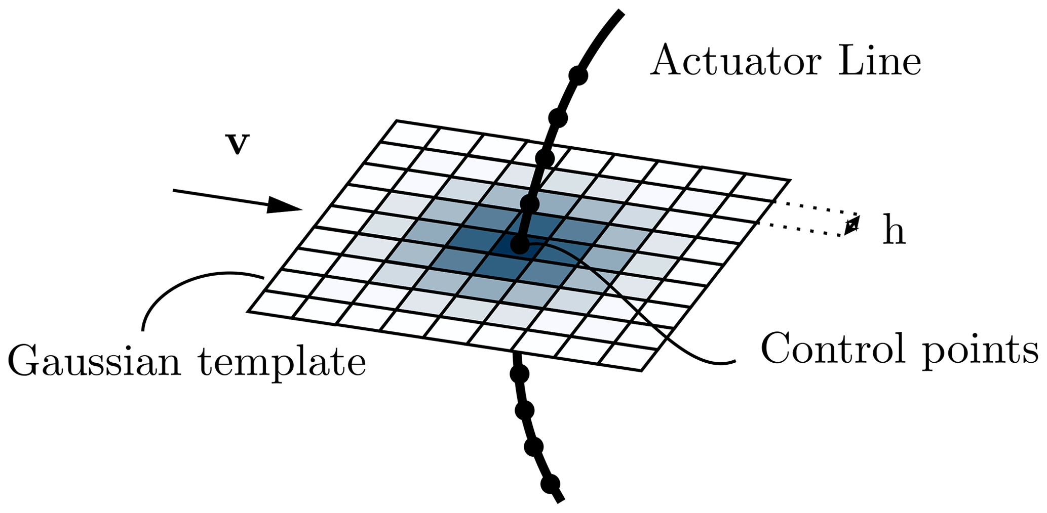
Figure 1 ALM with its associated template, with Gaussian weights used for the effective velocity sampling and the force distribution.

For aeroelastic simulations, the accuracy of the loads provided by the ALM is essential as they drive the structural dynamics. However, this accuracy is often questioned, especially at the blade tip, mostly due to the regularization of the forces that reduces the induced velocity. To mitigate this issue, it is possible to use either vortex-based smearing corrections (see Meyer Forsting et al., 2019; Dag and Sørensen, 2020; Martínez-Tossas and Meneveau, 2019; Kleine et al., 2023) or regularization kernels that lead to a more accurate prediction of the forces (Jha and Schmitz, 2018; Caprace et al., 2019). The second approach is employed here, using the 2D Gaussian regularization for both the evaluation of the effective velocity and the force distribution. This leads to a better estimation of the aerodynamic loads, hence decreasing the need for a smearing correction, especially when slender blades are considered. A more detailed description of the regularization used is provided in Trigaux et al. (2022), and its advantages over a 3D distribution are detailed in Caprace et al. (2019). Note that the shape of the tip vortices is affected by the type of mollification and that the use of a 2D mollification results in a sharp force gradient that can lead to numerical oscillations in some numerical methods. Here, these were verified to be of small amplitude and not to affect the flow dynamics away from these vortices and the loads on the blades. Here, the spatial resolution of the flow solver near the ALM is taken as 64 pts per turbine diameter D. Section 5 evaluates the influence of the resolution on the loads and the wake in the aeroelastic case.

2.3 Structural solver

The structural dynamics of the blades are simulated using the BeamDyn module from OpenFAST (Wang et al., 2017). BeamDyn implements nonlinear geometrically exact beam theory, which is particularly well suited to study slender blades made of composite materials as it accounts for the large displacements and allows for the coupling of degrees of freedom using full 6×6 cross-sectional mass and stiffness matrices. For the considered IEA 15 MW blade, this coupling mainly relates the flapwise and edgewise bending to the twist, which can substantially modify the angle of attack of the blade sections under classical loading conditions. The use of BeamDyn is justified by the importance of the nonlinear effects on large rotors (Manolas et al., 2015; Panteli et al., 2022). The structural data provided in Gaertner et al. (2020) are used. For this turbine, preliminary analysis indicates that the time step must be constrained by dt<0.005 s to correctly capture the dynamics of the first torsional mode. Each blade of the turbine is represented by one instance of the structural beam solver, for which the kinematics of the blade root is imposed. The simulations presented in this paper all consider a constant rotation speed, which decouples the blade root boundary condition from the other blades and drivetrain dynamics. The choice of a constant rotation speed is motivated by the need for exact comparison of the wake in different configurations, yet the absence of a model for the drivetrain dynamics impacts the rotor loads, as discussed in Sect. 4.2. Additionally, this approach allows us to use a larger time step than that typically used in OpenFAST simulations. BeamDyn is coupled to the ALM as described in the following section.

2.4 Coupling

The coupling scheme linking the flow and structural solvers is the second-order improved serial staggered (ISS) (Degroote, 2013), which is detailed in Fig. 2. This scheme evaluates the flow and the structural models at different time levels. The flow velocity is evaluated at time t and is used by the ALM to evaluate the aerodynamic forces based on the previous structural states $x(t-\mathrm{d}t/\mathrm{2})$ (the states include the blade deformation, position, and velocity). The structural response to these loads is then integrated in time, using sub-cycling (with constant forces) to meet the structural solver constraints on the time step. The forces are then re-evaluated by the ALM using the updated structural states and distributed on the flow mesh according to the deformed configuration.

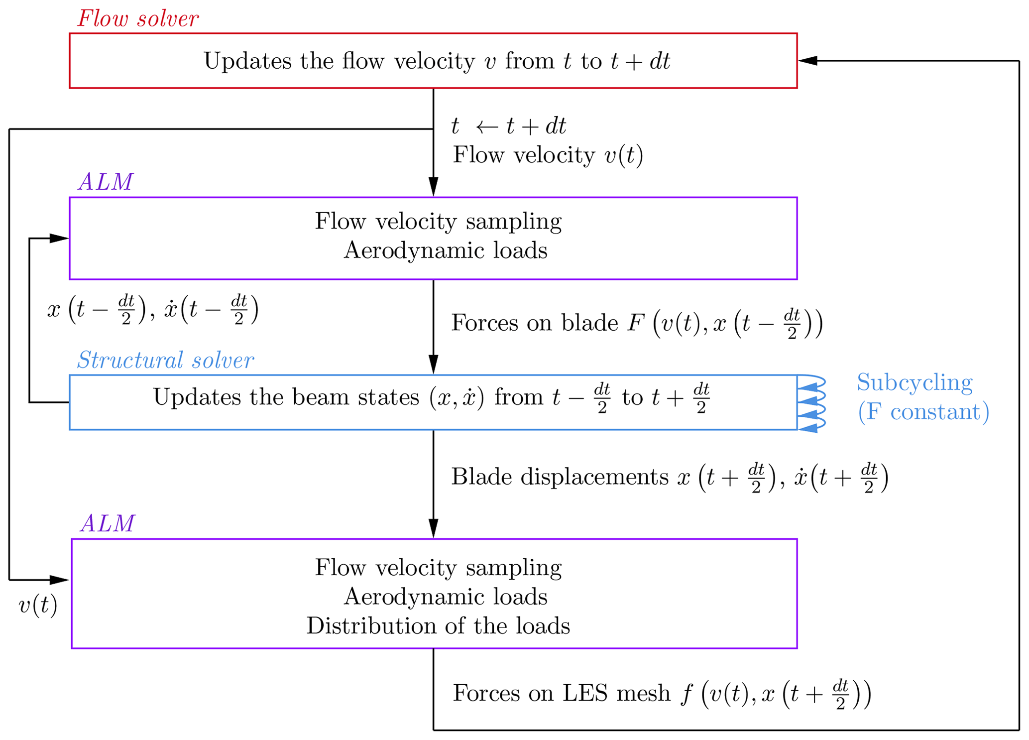
Figure 2 Schematic of the coupling between the flow and structural solver with the ALM as the interface.

The computational time required for solving the structural dynamics is much lower than that required by the flow solver. BeamDyn is very efficient thanks to the use of high-order spectral finite elements (Sprague and Geers, 2008). When the turbine operates at a constant rotation speed, the time step also remains relatively large, resulting in fewer necessary sub-steps. Additionally, here the structural dynamics of each blade is solved in parallel, leveraging the multiple CPUs dedicated to the flow solver that would otherwise remain in standby until the completion of the structural computation. As a result, the total overhead generated by using the structural solver is less than 5 % compared to simulations performed with rigid blades. More details on the implementation of the coupling between the ALM and the structural solver in parallel are provided in Appendix A.

The frames of reference in which the blade displacements, loads, and wake are presented are also defined according to Fig. 3. The global frame, in which the wake quantities are presented, is located at the tower bottom. The (${\widehat{\mathbf{e}}}_x$, ${\widehat{\mathbf{e}}}_y$, and ${\widehat{\mathbf{e}}}_z$) directions correspond to the streamwise, vertical, and lateral directions, respectively. The loads are presented in the blade root frame ${\widehat{\mathbf{e}}}_{\mathrm{b}}$. Its origin is located at the basis of the blade, and its orientation accounts for the shaft tilt angle, the blade rotation, and the cone angle. The displacements are also measured in the blade root frame and are considered to be the variation from the undeflected configuration. The torsion angle is defined along the ${\widehat{\mathbf{e}}}_{y,\mathrm{b}}$ axis such that a positive value of the angle corresponds to a nose-up rotation of the blade section.

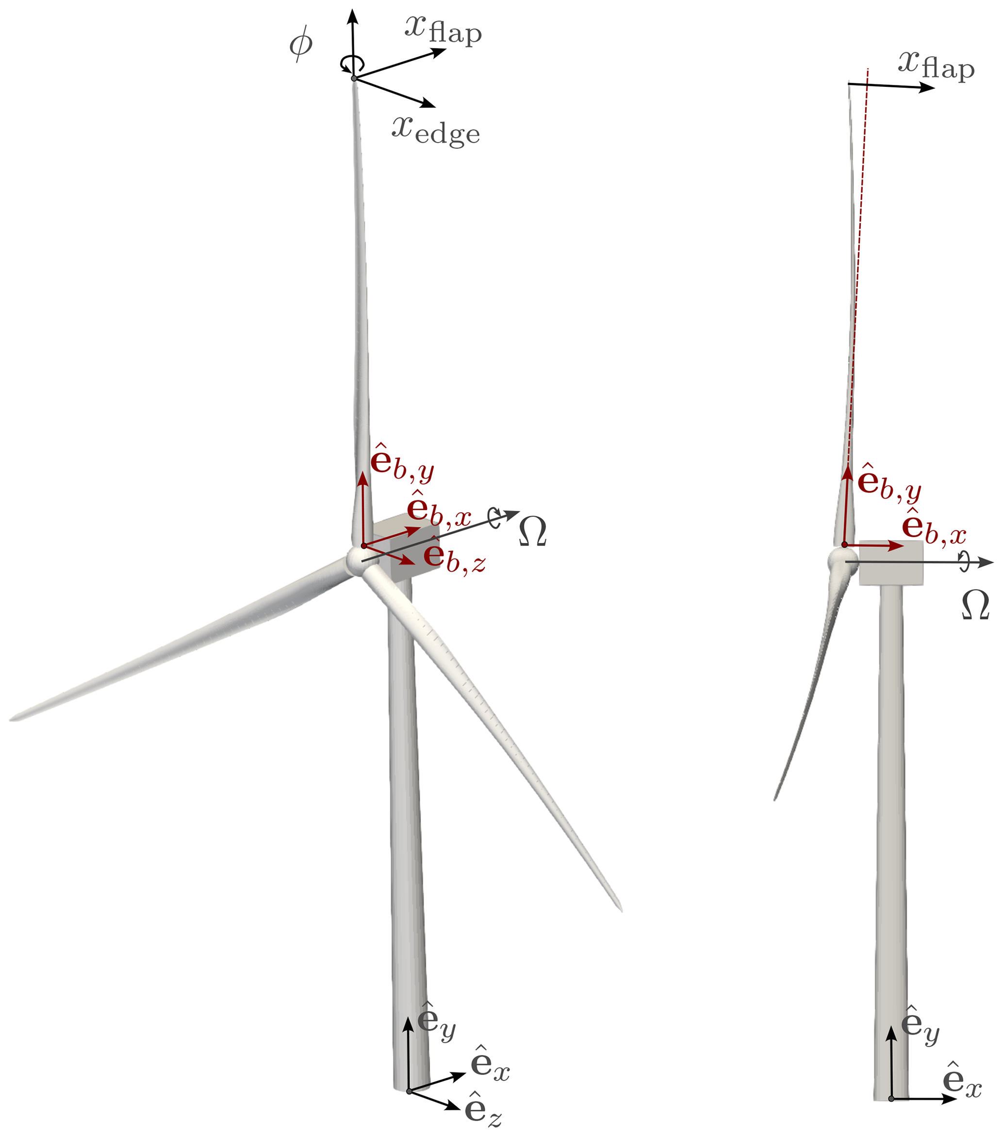
Figure 3 References frames: global frame (black arrow, $\widehat{\mathbf{e}}$) and blade root frame (red arrow, ${\widehat{\mathbf{e}}}_{\mathrm{b}}$). The rotor rotation vector Ω and the blade tip displacements (x_flap, x_edge, and ϕ) are also shown. The 3D turbine rendering is from OpenFAST.

The presented methodology allows us to simulate many rotations of wind turbines with flexible blades in LES at a reasonable computational cost (i.e. a few thousands of CPU hours for the simulations presented in the next section). In what follows, the methodology is compared to various aerodynamic models of OpenFAST before being applied to assess the effect of the flexibility on the IEA 15 MW turbine.

3 Comparison to the BEM theory and a free vortex wake model

The methodology developed in the previous section is tested and compared against the results obtained using different aerodynamic models available in OpenFAST (v3.5.0). OpenFAST is a publicly available modular framework that uses physics-based models to perform aero-servo-elastic simulations of wind turbines under various conditions (Jonkman, 2013). The presented comparison aims to verify our methodology and point out the limitations of some aerodynamic models for large wind turbines.

Here, the IEA 15 MW reference wind turbine is considered with the following parameters. The blades have a length of 117 m, and the hub radius is 3 m, leading to a total diameter D=240 m. To avoid tower strike, the blades are pre-bent by 4 m, the shaft is tilted by an angle of −6°, and the rotor has a cone angle of 4°. The gravity loads are also included. All the parameters used for this model are provided in the turbine definition, except for the structural torsional damping factor, which was increased to avoid torsional instabilities when the turbine operates in near-rated highly loaded conditions.

The following investigation compares the results obtained using the flexible ALM to those obtained using two aerodynamic models from OpenFAST: the blade element momentum (BEM) theory model and a free vortex wake model (cOnvecting LAgrangian Filaments, OLAF) (Jonkman et al., 2015; Shaler et al., 2020). BeamDyn is used for the blade structural dynamics in all the considered cases.

3.1 Comparison in uniform flow

First, the case of a uniform inflow is considered. The inflow wind speed is set to U_∞=9 m s⁻¹, which corresponds to the region of the controller where the optimal tip-speed ratio (TSR) of 9 is maintained. Consequently, the constant turbine rotation speed Ω is set to 6.45 rpm. The ALM and OpenFAST simulations run for 200 s, which corresponds to ≃21.5 rotations, and the results are averaged over the last four rotations. For the ALM simulations, the computational domain size is $\mathrm{12}D\times \mathrm{12}D\times \mathrm{12}D$ (in the streamwise, vertical, and transverse directions, respectively). The turbine is located at the position $(\mathrm{4},\mathrm{6},\mathrm{6}D)$ to ensure a sufficient distance from the domain boundaries. This way, the blockage ratio is ≃0.5 %, which allows us to compare the ALM simulations to the OpenFAST aerodynamic models that do not account for the presence of lateral boundaries. A uniform resolution of 64 flow grid points per diameter is used, and the time step is set to ≃0.025 s to obtain 360 time steps per turbine rotation. For the OLAF model, 50 blade nodes are used in the analysis, and the time step is set to 0.155 s, which corresponds to an azimuthal increment Δθ≃6° per time step, as suggested in the guidelines (Shaler et al., 2020). The circulation on the blade is obtained using the same airfoil polars as those used in the ALM. The near wake consists of 1024 vortex panels, which gives a wake length corresponding to approximately 17 rotations. There is no far-wake region. The last third of the wake is frozen to mitigate the effect of wake truncation. This wake length was verified to be sufficient in this case to provide a converged force distribution on the blades by comparing it to a simulation with a shorter near wake, using 600 panels extending for 10 rotations, which led to the same results. The vortex core is regularized using the Vatistas vortex model ¹ with the optimized parameter option, which corresponds to using r_c=2Δs, where Δs is the mean spanwise spacing between the aerodynamic nodes. The size of the regularization parameter can noticeably affect the force distribution, especially near the tip. The regularization also evolves with time using a viscous diffusion model (here with the parameter δ=1000). For the BEM, 50 radial locations are used. Prandtl's tip-loss factor is used to model the tip and the hub losses (Moriarty and Hansen, 2005). The tangential induction is accounted for in the BEM equations, and the effect of the drag term is considered in both the axial and the tangential induction. The OpenFAST cases have a very small time step of 0.0005 s, which is necessary to ensure the convergence of BeamDyn. Interested readers can refer to the IEA 15 MW definition that contains example cases with OLAF and the BEM (Gaertner et al., 2020).

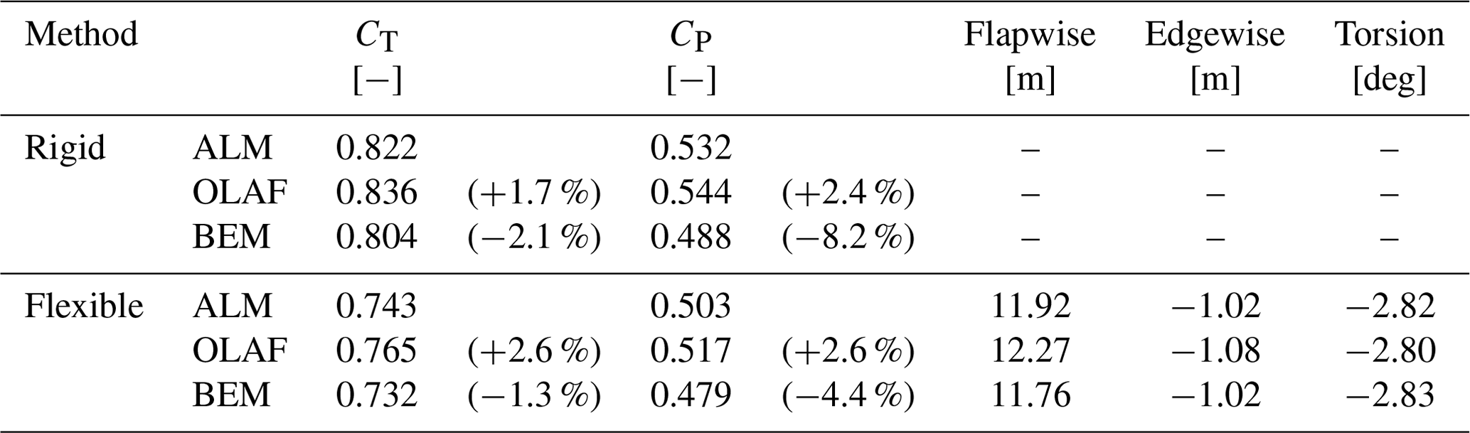
A comparison of the rotor thrust and power coefficients predicted by each method is provided in Table 1. For the rigid case, the thrust and power coefficients of the ALM and OLAF match well, whereas the BEM tends to predict a lower power coefficient. For the flexible case, the tip displacement is predicted similarly by all methods. These deflections are particularly significant in the flapwise direction, reaching a value of 12 m at the blade tip, which corresponds to around 10 % of the blade length. The torsion angle reaches −2.8° at the tip (corresponding to a nose-down rotation of the airfoil), which also significantly reduces the angle of attack of the blade section, resulting in a noticeable variation in the thrust and power coefficients when accounting for the blade flexibility. Specifically, all methods predict a 9 % decrease in the thrust coefficient. The variation in the power coefficient is closer to 5 % for the ALM and OLAF, whereas the BEM predicts a smaller reduction of 2 %. As a result, the difference in power coefficients between the methods is lower when flexibility is considered.

Table 1 Comparison of the time-averaged thrust coefficient (C_T), power coefficient (C_P), and tip deformation predicted by the various methods.

The aerodynamic forces acting on the rigid and flexible blade are displayed in Fig. 4. These forces are expressed in the blade root frame. For the rigid case, the forces obtained using OLAF and the ALM match very well. The only noticeable difference between the two methods is the small increase in the forces near the blade tip, which is more pronounced using OLAF. The latter is due to the regularization of the trailing vortex filaments, which decreases the induced velocity near the tip. To a smaller extent, the ALM also depicts a slight increase in the lateral forces (i.e. F_z, in the blade root frame) at the tip due to the mollification (i.e. the smearing of the shed vortices, Caprace et al., 2019). It is however less pronounced thanks to the use of the 2D mollification, without spanwise smearing. The force distribution predicted by the BEM is lower than for OLAF and the ALM, especially in the edgewise direction. This difference was also observed in other studies (Madsen et al., 2012; Perez-Becker et al., 2020) and can be explained by two factors. High thrust coefficients are somewhat challenging for the BEM as the limits of the validity of the theoretical model are reached, and the empirical Glauert correction is used. On the other hand, the mollification of the ALM and the regularization of the vortex core in OLAF also affect the induction, which can result in slightly higher forces (Caprace et al., 2019; Shaler et al., 2023).

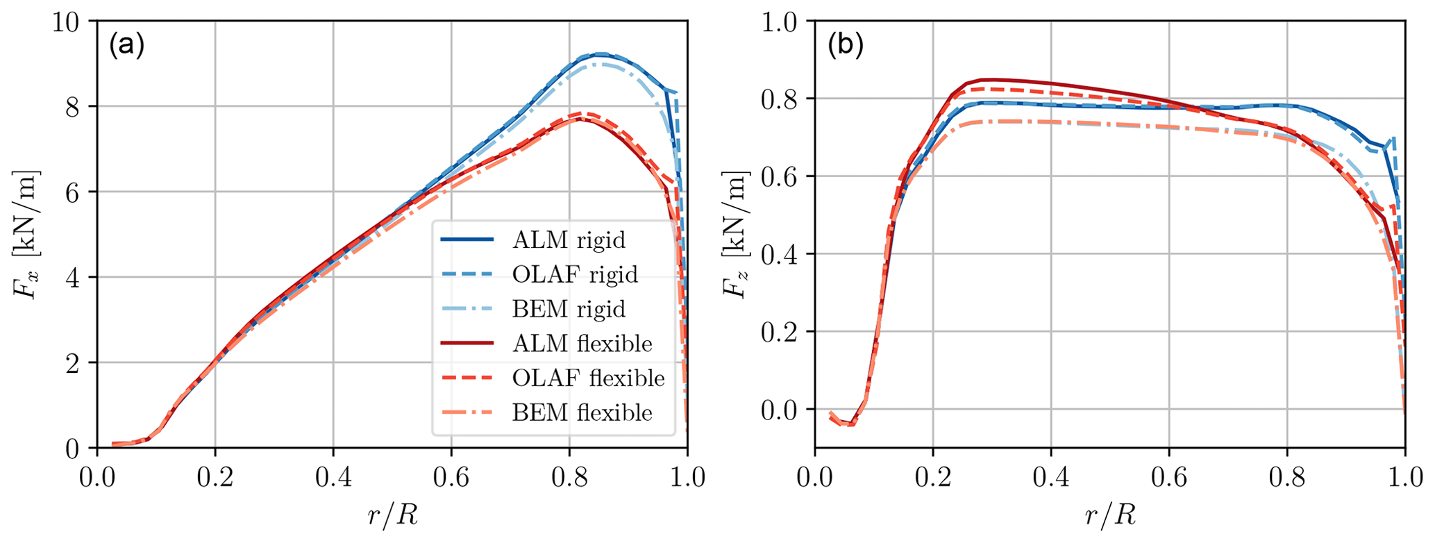
Figure 4 Steady-state aerodynamic loads in the blade root frame for the rigid (blue lines) and flexible (red lines) cases: ALM (dark solid line), free vortex wake model OLAF (dashed line), and the BEM (light dashed–dotted line) from OpenFAST. Normal (F_x, a) and lateral (F_z, b) forces (relative to the blade root frame).

When flexibility is considered, all methods predict a significant decrease in the loads on the outer part of the blade ($r/R>\mathrm{0.6}$). This decrease is more significant for OLAF and the ALM than for the BEM, especially in the edgewise direction. This difference arises from the fact that the BEM predicts less change in the axial induction due to the out-of-plane bending. Conversely, the effect of the torsion angle is captured similarly by all methods, which results in a similar load distribution in the flapwise direction. Additionally, on the inner part of the blade ($r/R<\mathrm{0.5}$), OLAF and the ALM show an increase in the loads. This phenomenon arises from the additional flapwise deformation of the blade, which modifies the location of the emission of the tip vortices, and was also observed to a smaller extent for the NREL 5 MW turbine (Dose et al., 2018; Trigaux et al., 2022). It is not captured by the BEM as the effect of the blade curvature on its aerodynamics is not modelled here (Fritz et al., 2022; Li et al., 2022). These findings are also consistent with the results predicted by the BEM and blade-resolved URANS simulation for the DTU 10 MW turbine presented in Sayed et al. (2019). This highlights the importance of using higher-fidelity methods when the aeroelasticity of large rotors is considered or at least considering the effect of out-of-plane bending on the blade aerodynamics (Fritz et al., 2022; Li et al., 2022), also for steady loads such as those presented in this section.

3.2 Comparison in turbulent flow

To verify the dynamic response of the structure under unsteady loads, a comparison between our framework and OpenFAST is also carried out with a turbulent inflow. The latter consists of the superposition of a uniform flow with U=9 m s⁻¹ and a turbulent field generated using the Mann algorithm (Mann, 1998). The parameters of the turbulent field are the integral length scale, here set to L=88.5 m; the anisotropy factor Γ=3.9; and the turbulence intensity, set to TI =6 %. The turbulent fluctuations are generated in a 3D domain of size $\mathrm{8}D\times \mathrm{2}D\times \mathrm{2}D$, with a spatial discretization of 32 points per D. In OpenFAST, the turbulent fluctuations are directly interpolated from the 3D domain to the turbine blade nodes and added to the upstream velocity value. In the case of the ALM, the turbulent fluctuations are interpolated to the inflow plane and are then convected to the turbine location. The OpenFAST cases are kept identical to the cases with a uniform inflow. Only the time step at which OLAF emits a new panel is decreased to 0.1 s to better account for the turbulent fluctuations. The ALM case also remains identical, except that the distance between the turbine and the inflow plane is reduced to 2 D to reduce the variation in the turbulent fluctuations that occurs during their convection from the inflow to the turbine. The cases are run for 400 s to converge the statistics.

The dynamic structural deformation of the blade is considered for this comparison to assess whether the flexible ALM correctly captures the variations in the displacements at the relevant frequencies. Figure 5 depicts the power spectral density (PSD) of the tip displacement for the flapwise and edgewise translations and for the torsion angle. The PSDs are computed using the Welch algorithm with segments of duration equal to 50 s that overlap by half their length (Welch, 1967). The blade natural frequencies are also depicted. These were obtained using the mass and stiffness matrices provided by BeamDyn in the rotating undeformed configuration, without accounting for the coupling with the aerodynamic loads. It should be noted that, for a nonlinear beam solver such as BeamDyn, the blade natural frequencies are slightly affected by the deformation. Here, this difference was verified to be negligible such that the natural frequencies do not need to be updated using the blade deformed configuration. Very good agreement is observed between OpenFAST and the ALM. All the methods predict the same magnitude for the peak occurring at the 1P frequency for all three components. Additionally, the peaks of displacement occurring at the edgewise natural frequencies (E1 and E2) are present and reach the same value for all three solvers. The structural response close to the first torsional frequency (T1) is also similar for all methods. All three solvers predict a similar decrease in the frequency at which this peak arises compared to the T1 frequency. This shift is due to the coupling between the aerodynamic forces (that increase linearly with the angle of attack) and the torsion angle. The amplitude of the peak is however slightly smaller for the ALM. Indeed, the values of the PSD at all the higher frequencies (larger than 20P) obtained using the ALM are smaller than those predicted using OpenFAST. This is mostly related to the use of integral velocity sampling for the ALM, which leads to some smoothing of the fluctuations as the velocity is obtained as a weighted average. In contrast, OpenFAST interpolates the velocity fluctuations directly to the nodes of the aerodynamic solver (BEM or OLAF). However, the amplitude of these differences is limited, and the value of the PSD at the affected frequencies is much smaller than at the lower frequencies, which are predominant. Some additional differences in the lower-frequency part of the spectrum are related to changes in the turbulent field during its convection from the inflow to the turbine location.

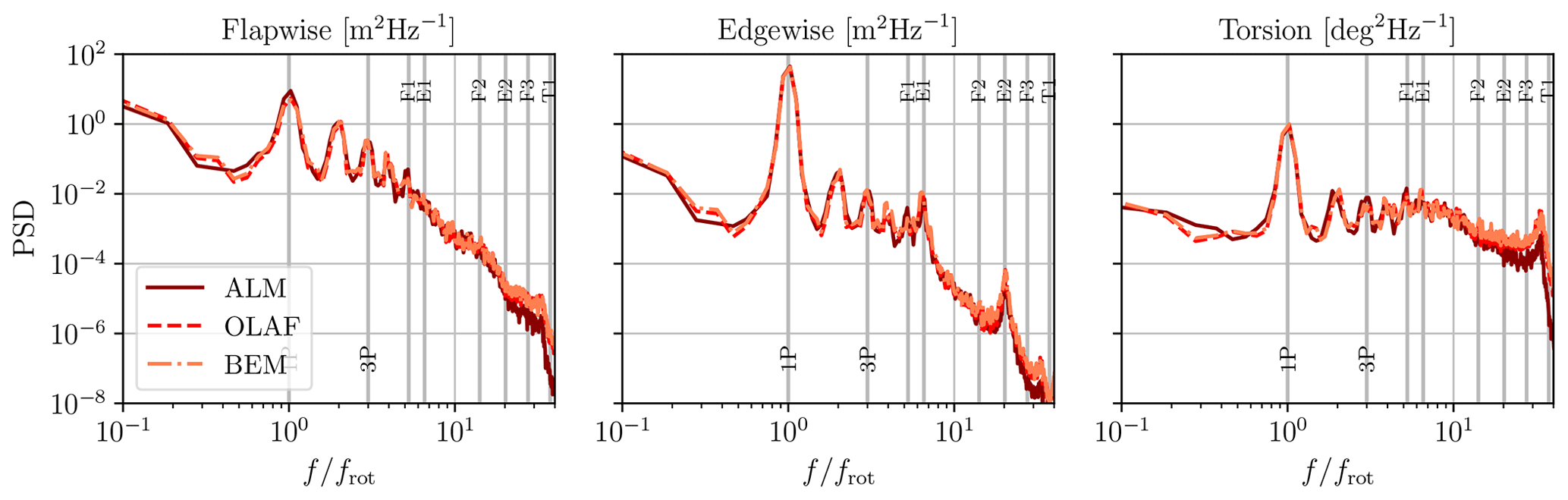
Figure 5 PSD of the tip displacement in the flapwise and edgewise directions and torsional deformation. Comparison between the ALM (dark solid line), OLAF (dashed line), and the BEM (light dashed–dotted line). The vertical lines denote the main frequencies of the system (1P and 3P), and the flapwise (F), edgewise (E), and torsional (T) natural frequencies.

4 Investigation of rigid and flexible rotors in atmospheric conditions

In this section, rigid and flexible rotors are studied with sheared turbulent wind as inflow to evaluate the unsteady aeroelastic effects on the aerodynamic loads and the wake. To this end, the numerical setup consists of a domain size of $\mathrm{12}D\times \mathrm{4}D\times \mathrm{4}D$, with a spatial resolution of 64 grid points per D. The location of the turbine hub is $(\mathrm{2}D,y_{\mathrm{hub}},\mathrm{2}D)$, where y_hub=150 m. Although the distance between the turbine and the inflow is small, it has been verified to have a very small effect on the loads (approximately 1 % difference in thrust and 3 % difference in power when the distance to the inflow is doubled). Moreover, the same distance to the inflow is used for each considered case such that the comparison is not affected. To ensure a valid comparison between the rigid and flexible cases, the rotation speed at the blade root is set to Ω=0.75 rad s⁻¹, which corresponds to the design TSR of 9. The time increment of the flow simulation is set to obtain 360 time steps per turbine rotation. Additionally, there are four structural sub-steps per flow time step. A total of 200 rotations are simulated for each case, which corresponds to a physical time of 1675 s.

The inflow is a neutral ABL generated using the co-simulation technique (as described in Sect. 2.1). The numerical setup is described in detail in Appendix B. It was designed to obtain a time-averaged velocity of U_hub=10 m s⁻¹ at hub height and with a TI close to 5 %. The obtained profiles of mean velocity and turbulence intensity are also provided in the Appendix, together with the methodology used to estimate the integral length scales, obtained as 106 m in the streamwise direction and 89.5 m in the lateral direction.

Three cases are compared in this section. The first case is the “rigid undeformed” rotor, which includes the upwind pre-bend of the blades. The second case is the flexible rotor, modelled using the flexible ALM that dynamically deforms based on the aerodynamic loads. The third case considers a rigid rotor that includes the mean deformation of the blades, noted as the “rigid deformed” case. The deformed geometry was obtained by time averaging the structural displacements obtained in the second case. This allows us to isolate the effect of the time-varying response of the blade on the rotor dynamics and wake.

This analysis is structured in three parts. First, the displacements of the blades are considered. Then, the distribution of the loads and their variation are presented. Understanding these aspects allows us to explain the differences observed in the wake, which are presented in the last part of the analysis.

4.1 Structural displacements

The PSD of the displacements is first considered in Fig. 6. In this section, the presented statistics of the blade displacements and loads are computed using the last 180 rotations of the simulations. The first 20 rotations are discarded as the wake induction has not yet converged. The power, thrust, and power spectra of the loads were verified to have reached statistical convergence after 20 rotations. The presented PSDs are computed using the Welch algorithm. The time series are divided into sub-segments of length equal to 22.5 rotations that overlap by half their length, resulting in a total of 15 segments. The PSDs are also computed for each blade and then averaged, resulting in smooth spectra. For all the components of the displacement, the 1P frequency is the most noticeable, as also noted for smaller turbines in Grinderslev et al. (2021). In the flapwise direction, the 1P frequency is excited by the rotation of the blade in the mean shear and in the spatially coherent turbulent structures. For the edgewise direction, the excitation of the 1P frequency is mostly attributed to gravity. In this direction, the spectrum reaches a much higher value at 1P than at the other frequencies, indicating the dominance of gravity over the aerodynamic loads. In the torsional direction, the peak at 1P is due to the coupling with the translational degrees of freedom and the effect of gravity on the deformed blade. The harmonics of the rotation frequency are also significant in all spectra, which is consistent with the results of Krüger et al. (2022). Concerning the blade structural frequencies, their excitation depends on the considered component. In the flapwise direction, the PSD exhibits no particular excitation at the flapwise (F1, F2, or F3) frequencies. Only a small peak is visible near the torsional frequency. The absence of a peak is explained by the high aerodynamic damping of the flapwise mode (Hansen, 2007). This damping is due to the fact that the blade flapwise displacement decreases the apparent streamwise velocity on the blade section, hence decreasing the angle of attack and the loads. In contrast, in the edgewise direction, distinguishable peaks of displacement occur at the edgewise natural frequencies (E1, E2) and close to the torsional frequency (T1). This is a result of the small aerodynamic damping in this direction, yet the amplitude of the peaks remains small compared to the one occurring at 1P. For the torsional direction, a peak occurs slightly below the T1 frequency, as observed in Sect. 3.2.

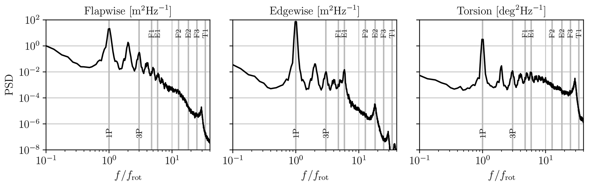
Figure 6 PSD of the tip displacement in the flapwise and edgewise directions and PSD of the tip torsion angle, for the IEA 15 MW turbine with flexible blades in atmospheric conditions. The vertical lines denote the main frequencies of the system (1P and 3P), and the flapwise (F), edgewise (E), and torsional (T) natural frequencies.

It is also interesting to consider the general shape of the displacement spectra. In the flapwise direction, the PSD follows a general downward slope that is constant throughout most of the spectrum. In the edgewise direction, a similar trend is noticeable before the 1P frequency and between the E1 and T1 frequencies. However, for the first harmonics of 1P, the general trend of the PSD remains constant. For the torsional direction, the general shape of the spectrum remains constant across the frequencies. Consequently, in this direction, some non-negligible high-frequency modes are observed in addition to the rotation frequency.

As the rotational frequency appears to be predominant, it is interesting to investigate the variation in the displacements along one rotation. The mean displacement and standard deviation are represented in Fig. 7 as a function of the azimuthal angle (with 0 representing the blade pointing upward). The values measured at each angle and over the simulated turbine rotations are also plotted; for each angle, they can be viewed as an approximation of the probability density function (PDF). In the flapwise direction, the minimal blade displacement is reached a few degrees after the blade's downward position. In this region, the PDF also has the smallest spread. Interestingly, the maximal mean flapwise displacement is not reached at the blade's upward position (i.e. 0°), where the flow velocity is maximal, but is rather constant from 0 to 90°. A similar behaviour was also observed for a 5 MW turbine by Santo et al. (2019). The PDF also exhibits a larger spread when the blade is in the upper-half region (i.e. between 270 and 90°). Overall, the flapwise deformation varies significantly along the rotation, oscillating between 12.4 and 13.6 m, primarily due to the mean shear of the flow. This displacement also represents more than 10 % of the rotor radius, which is quite significant, and illustrates the increased blade flexibility compared to smaller turbines. The PDF also reveals large variations around the mean displacement, attributable to the turbulent fluctuations. In contrast, the edgewise displacement presents a nearly perfect sinusoidal variation that is consistent with the gravity loads (Höning et al., 2024). The spread around the mean is also very limited, as the variation in the aerodynamic loads is small compared to that of the gravity. The torsional deformation follows the same phase as the edgewise displacement. This is due to the effect of the gravity loads and the flapwise deformation, which generates a torsion moment on the structural reference axis. Consequently, the torsion angle differs between the left and right parts of the rotor, which can lead to some additional load imbalance. The PDF also presents a larger width than for the edgewise displacement as a result of the higher sensitivity to the turbulent fluctuations.

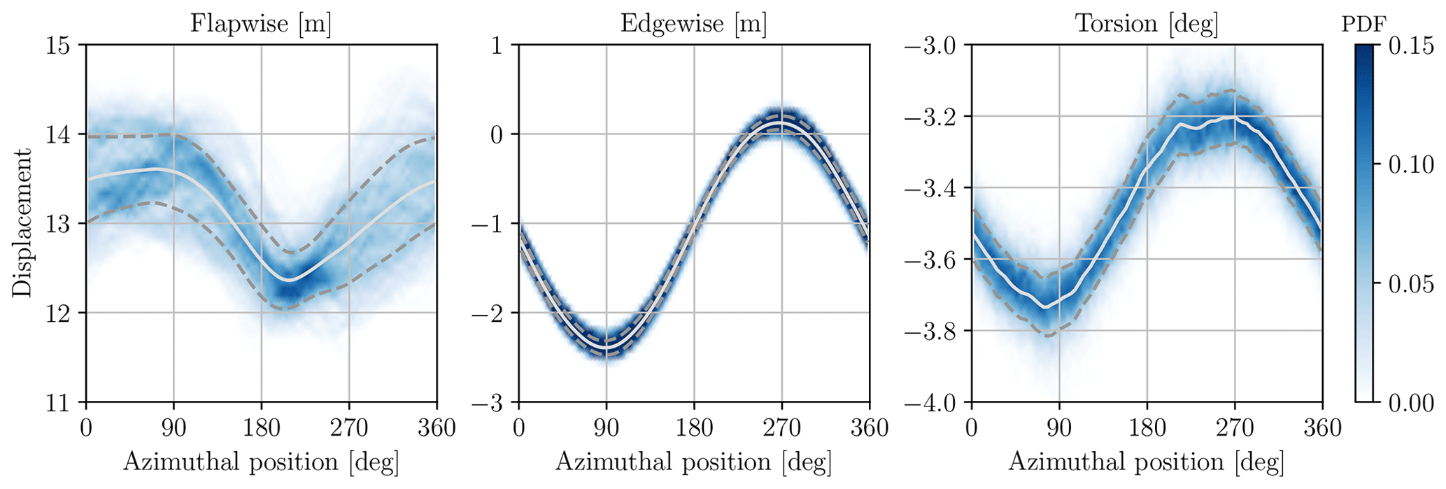
Figure 7 Tip displacement: mean (solid line), standard deviation (dashed line), and values encountered over the turbine rotations (blue shading, approximating a PDF) as a function of the blade azimuthal angle (as measured from the blade's upward position).

The flapwise structural velocity is also considered as it substantially affects the angle of attack and hence the aerodynamic forces. In fact, the angle of attack α of a section of the blade can be approximated using the flow and structural velocities expressed in the blade root frame by neglecting the effect of the blade curvature on the angle of attack,

$$\begin{array}{}\text{(1)}& \mathit{\alpha }\simeq \arctan \left({\displaystyle \frac{\left(v_x-v_{\mathrm{struct},x}\right)}{\left(v_{\mathrm{struct},z}-v_z\right)}}\right)+{\mathit{\varphi }}_{\mathrm{struct},y}+\mathit{\beta },\end{array}$$

where v_x and v_z are the local flow velocities in the x (streamwise) and z (azimuthal) directions, v_struct,x and v_struct,z are the local structural velocities in these directions, ϕ_struct,y is the local torsion angle, and β is the local twist angle. Here, all these variables are expressed in the blade root frame. In general, the structural velocity in the z direction mostly consists of the rotational velocity Ωr, and the flow velocity is also negligible in comparison, leading to $\left(v_{\mathrm{struct},z}-v_z\right)\simeq \mathrm{\Omega }r$. Additionally, since the normal velocity is also much smaller than the rotational velocity, $\arctan (\left(v_x-v_{\mathrm{struct},x}\right)/(\mathrm{\Omega }r\left)\right)\simeq \left(v_x-v_{\mathrm{struct},x}\right)/\left(\mathrm{\Omega }r\right)$. As a result, the expression for the angle of attack is simplified to

$$\begin{array}{}\text{(2)}& \mathit{\alpha }\simeq {\displaystyle \frac{\left(v_x-v_{\mathrm{struct},x}\right)}{\left(\mathrm{\Omega }r\right)}}+{\mathit{\varphi }}_{\mathrm{struct},y}+\mathit{\beta }.\end{array}$$

Consequently, the ratio $v_{\mathrm{struct},x}/\left(\mathrm{\Omega }r\right)$ has an effect on the angle of attack that is similar to that of the torsion angle. Figure 8 shows the mean flapwise velocity v_struct,x has a function of the blade azimuthal angle and the probability density function for each angle. The maximal positive velocity is 0.4 m s⁻¹ and is reached in the left region of the rotor. The minimal velocity is −0.7 m s⁻¹ and is reached when the blade is pointing downward. These values are more significant than those reported in Santo et al. (2019) for a 5 MW turbine in atmospheric conditions, which illustrates that the maximal flapwise velocity reached along the rotation likely increases with the rotor size. A large variation in the velocity occurs around the blade's downward position, which is attributed to the high mean vertical shear in the lower region of the rotor. The PDF of the flapwise velocity is also quite large around the mean, due to the turbulent fluctuations of the velocity. The figure also shows the contribution of the flapwise velocity ($-v_{\mathrm{struct},x}/\left(\mathrm{\Omega }r\right)$) to the variation in the angle of attack at the tip along a rotation. It is compared to the contribution of the torsional angle (${\mathit{\varphi }}_{\mathrm{struct},y}-{\stackrel{\mathrm{‾}}{\mathit{\varphi }}}_{\mathrm{struct},y}$). The two effects are similar in magnitude and can result in a small variation in the angle of attack of up to 0.4°. Their phase is shifted by a quarter rotation, as the effect on the flapwise velocity mostly depends on the vertical shear, whereas the variation in the torsion follows the same phase as the edgewise displacements (and hence the gravity loads).

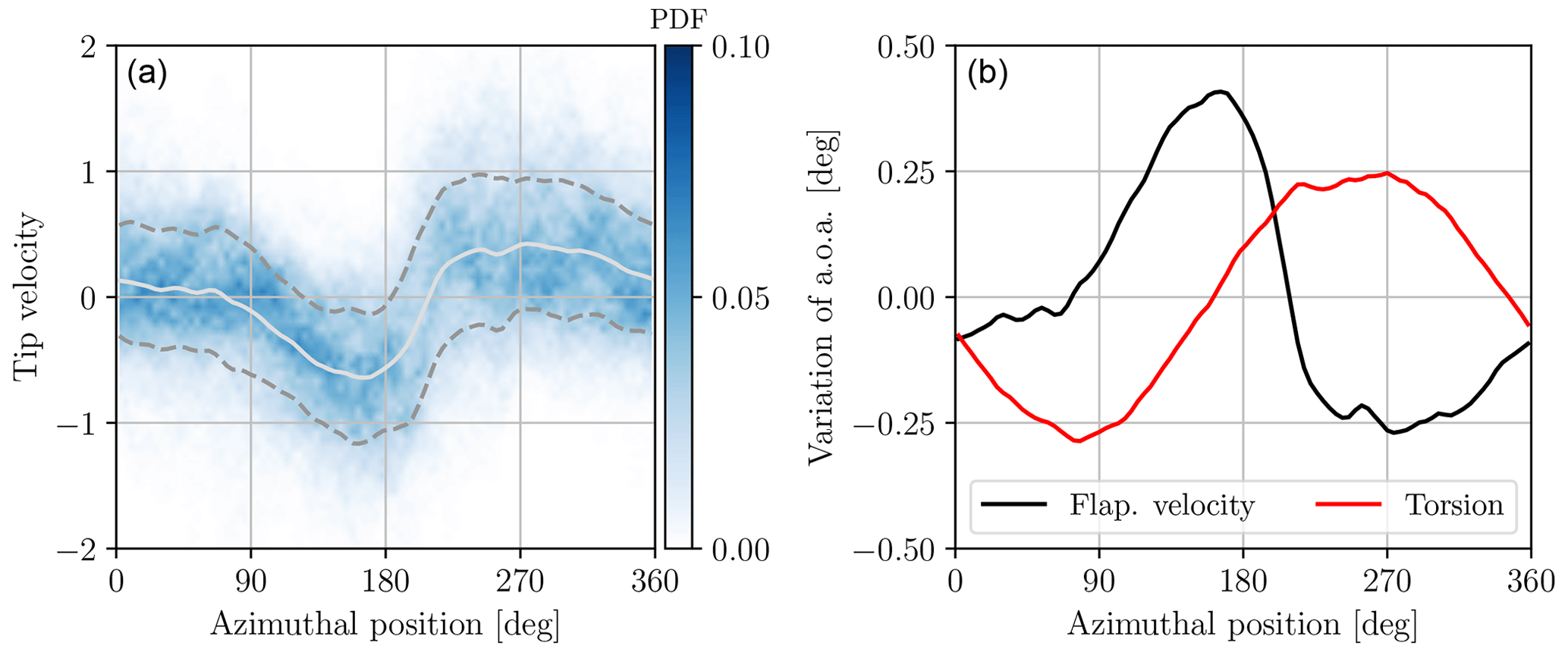
Figure 8 (a) Flapwise structural velocity at the tip: mean (solid line), standard deviation (dashed line), and values encountered over the turbine rotations (blue shading, approximating a PDF) as a function of the blade azimuthal angle. (b) Comparison of the impact of the flapwise velocity $-v_{\mathrm{struct},x}/\left(\mathrm{\Omega }r\right)$ and the torsion angle (${\mathit{\varphi }}_{\mathrm{struct},y}-{\stackrel{\mathrm{‾}}{\mathit{\varphi }}}_{\mathrm{struct},y}$) on the angle of attack.

These displacements are not without consequences for the loads acting on the turbine, which are presented in the next section.

4.2 Comparison of the blade loads

This section presents a comparison of the loads obtained with the flexible and rigid rotors. Here, the focus is on the blade loads, presenting both the aerodynamic loads due to their impact on the wake and the structural loads due to their effect on the structural integrity. This choice also follows from the decision to maintain a constant rotation speed, primarily to facilitate the comparison between the wakes. In real-world conditions, the turbine controller adjusts the rotation speed and the blade pitch angle, and the three blades are dynamically coupled by their rigid connection with the turbine shaft, which modifies the resulting rotor loads, especially the rotor torque. To assess the impact of these changes, the simulations were also conducted with the controller. The loads and displacements of the individual blades were not noticeably affected and neither was the wake. However, the spectrum of the rotor torque was modified due to the coupling between the blades and the generator. Consequently, we chose to present the simulation at a constant rotation speed and to focus on the individual blade dynamics and the wake, which were confirmed to remain mostly unaffected by the controller.

First, the mean load distribution along the blade, depicted for each case in Fig. 9, is examined. The load distribution on the undeformed rotor clearly differs from that of the two cases that include the deformation. In particular, a significant reduction in the mean loads and their standard deviation is induced by the structural displacement on the outer part of the blade. This results in a substantial reduction in the power and thrust coefficients. The thrust coefficient is reduced by ≃ 14 %, going from C_T=0.80 for the undeformed rotor to C_T=0.69 for the deformed cases. Similarly, the power coefficient is reduced by 10 %, from C_P=0.50 to C_P=0.45. As anticipated, the rigid deformed and flexible cases exhibit a nearly identical mean force distribution. However, in the flexible case, the standard deviation presents a slight reduction, attributable to the additional compliance of the blade.

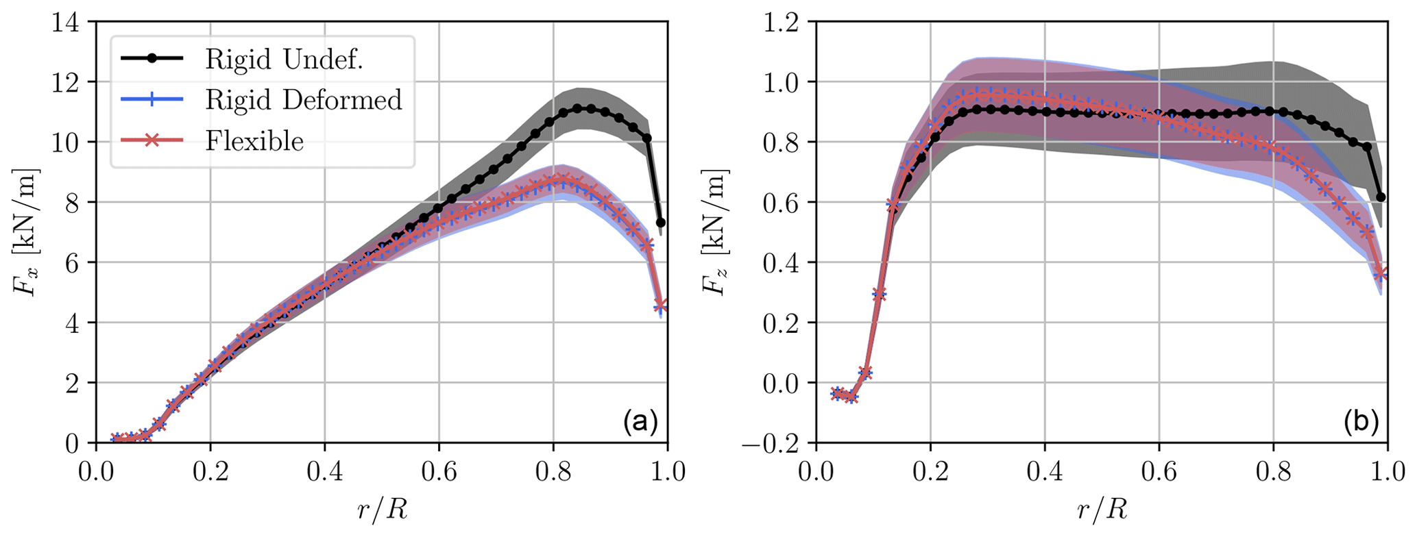
Figure 9 Distribution of the aerodynamic loads along the blade span for the rigid undeformed (black line), rigid deformed (blue line), and flexible (red line) cases. The shaded area represents the standard deviation. (a) Flapwise forces; (b) edgewise forces.

Although the radial distribution of the forces is the same for the rigid deformed and flexible cases, their distribution over the rotor plane varies. Figure 10 depicts the difference between the force distribution of the two cases. There is a notable difference at the bottom of the rotor in both the flapwise and the edgewise directions. In this region, the flexible rotor experiences more force due to the reduced flapwise deflection and the significant upstream blade velocity that increases the angle of attack, as observed in Fig. 8. In the normal direction, there is also a clear asymmetry between the left and right planes of the rotor. The flexible rotor presents higher forces compared to the rigid rotors on the left part of the plane due to the smaller torsion angle on this side. This asymmetry is not visible in the edgewise direction. The observed differences reach a maximum of around 10 % on the lower part of the rotor plane, which also results in a difference in the mean velocity deficit in the near wake, as discussed in the next section.

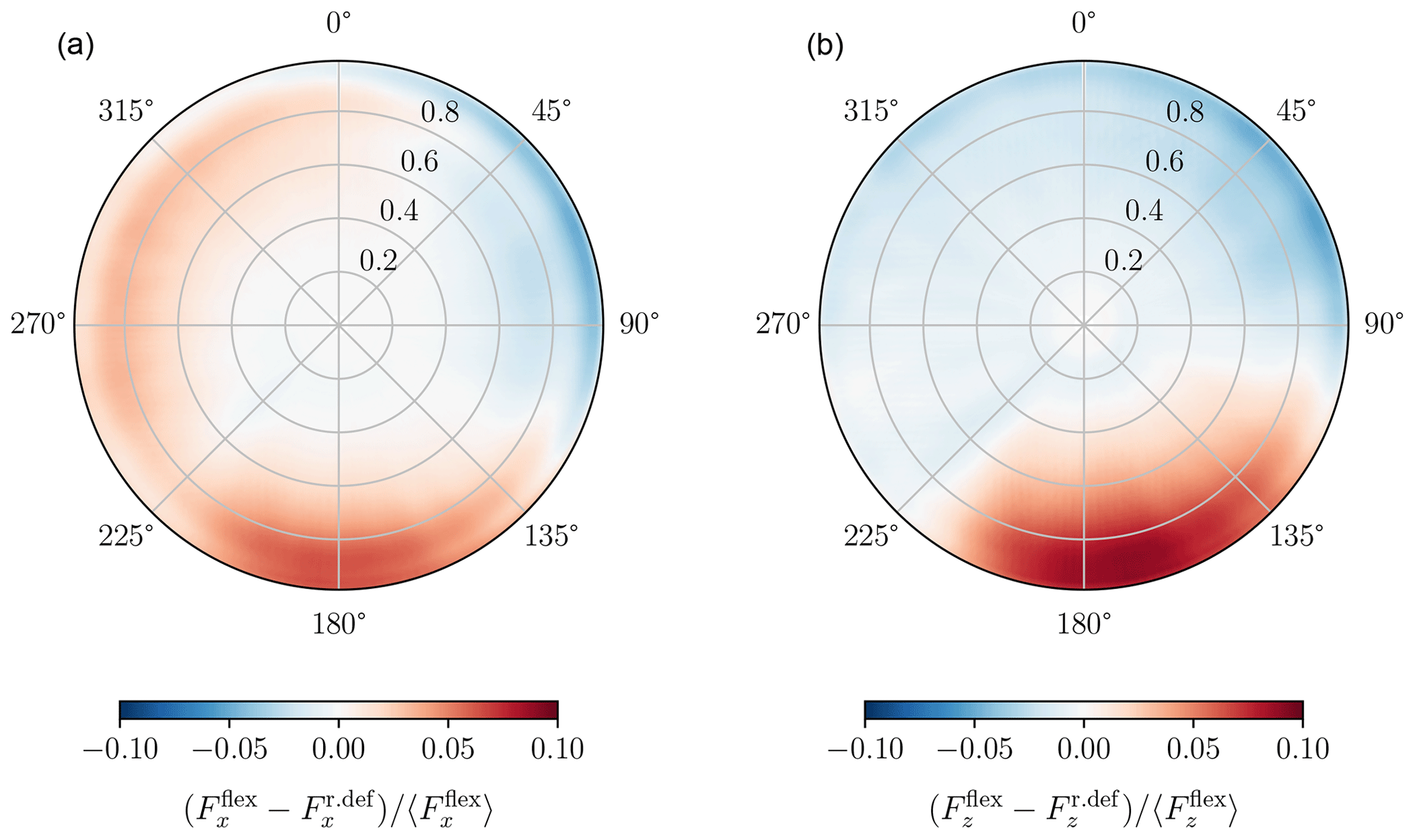
Figure 10 Difference between the aerodynamic force distribution of the flexible case (F^flex) and the rigid deformed case (F^r.def) on the rotor plane (front view), normalized by the mean force on the rotor. (a) Flapwise forces; (b) edgewise forces.

Figure 11 presents the PSD of the blade root moment in the two main directions. The spectra are given for the aerodynamic forces and the elastic structural response (which includes the inertia, centrifugal force, and gravitational force). Considering first the aerodynamic forces, one observes that the rotation frequency is still the most important component. The amplitude of the PSD at this frequency differs slightly between the cases, with the rigid undeformed case having the highest value and the flexible case the lowest. Large differences also appear close to the natural frequencies. The PSD is much lower close to the main bending frequencies (F1, E1) due to the dynamic response of the blade. In fact, at these frequencies, the blade responds significantly to the variations in the forces, and the resulting structural bending tends to smooth these changes. There is also a noticeable increase at the torsional frequency (close to T1) due to the subsequent modification of the angle of attack of the blade. The structural moment does not exhibit a decrease at the bending frequency, as the lower aerodynamic forces are compensated for by the inertial loads. In the flapwise direction, the spectrum of this moment is generally slightly smaller in the flexible case. There are also no specific peaks at the natural frequencies due to the high aerodynamic damping in this direction. In contrast, the edgewise root moment presents high peaks close to its natural frequencies. In this direction, the value of the PSD at the 1P frequency is also much higher than that of the aerodynamic loads, illustrating the importance of the gravity loads. The modification of the spectrum of the root moment can have a direct impact on the lifetime of the turbine and the damage equivalent load calculations, as also noted in Hodgson et al. (2021). It is therefore necessary to consider dynamic models when assessing the structural integrity of the rotor.

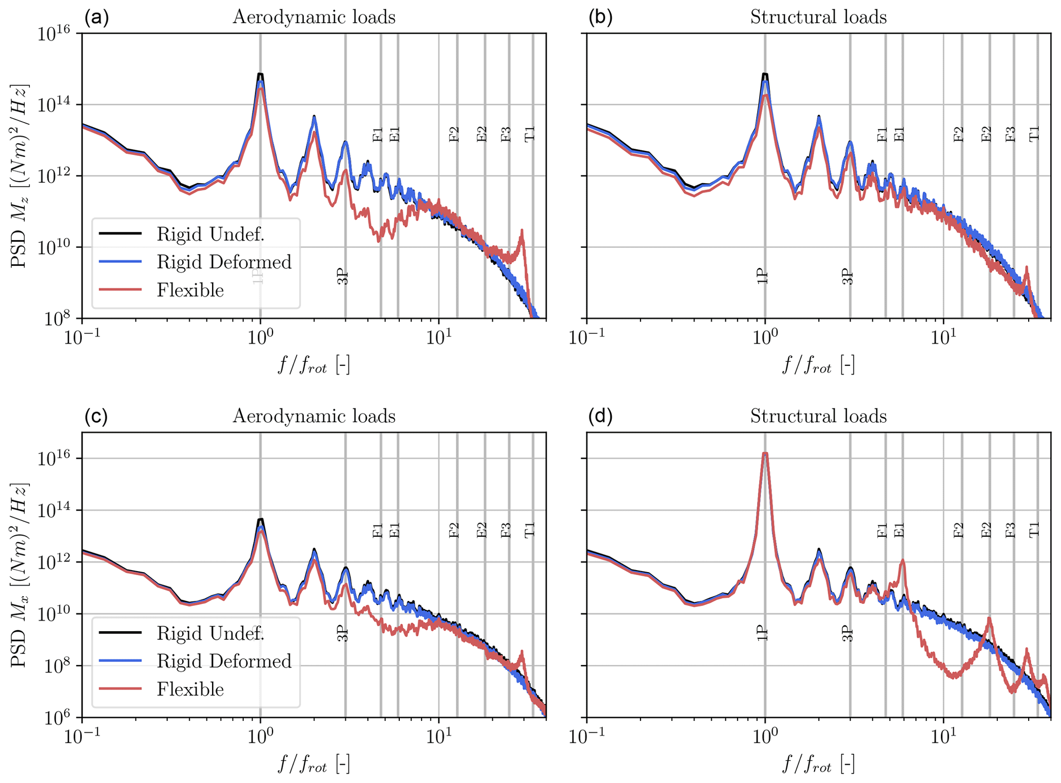
Figure 11 PSD of the blade root moment due to the flapwise forces (M_z, a, b) and edgewise forces (M_x, c, d). (a, c) PSD of the moment of the aerodynamic loads; (b, d) PSD of the structural root moment. Comparison between the rigid undeformed (black line), rigid deformed (blue line), and flexible (red line) cases.

Similarly to the displacement, the variation in the blade root moment of the aerodynamic forces along the rotation is further investigated, as the 1P frequency was shown to be the most significant. The latter is represented in Fig. 12. The aerodynamic forces, rather than the structural response, are considered to remove the influence of gravity, which would be dominant on the edgewise moment.

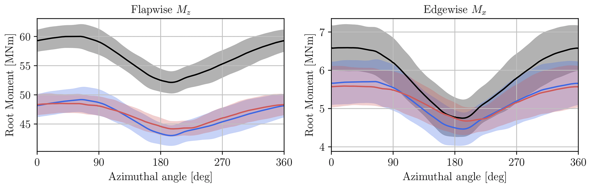
Figure 12 Blade root moment of the aerodynamic forces as a function of the azimuthal angle and averaged over the turbine rotations: mean value (solid line) and standard deviation (shaded area). Comparison between the rigid undeformed (black line), rigid deformed (blue line), and flexible (red line) cases.

The mean flapwise moment acting on the rigid turbine is 21 % higher than that obtained in the cases that include the deformation, which have a comparable mean value. The amplitude of the deviation along the rotation, defined as $(M_{\max }-M_{\min })/M_{\mathrm{mean}}$, is however similar in both rigid cases (14.0 % for the rigid undeformed case and 13.2 % for the rigid deformed case). This deviation is reduced to 9.3 % in the flexible case, mostly due to a higher minimal value when the blade is in its downward position. In the edgewise direction, the mean value of the root moment is 12 % higher in the rigid undeformed case. The deviation is 31.5 % in this case, compared to 23.7 % in the rigid deformed case and 17.5 % in the flexible case.

Interestingly, there is also a noticeable phase lag between the rigid and the flexible cases. While the rigid case predicts a minimal moment at around θ=195°, the flexible case predicts a minimum at θ=215°. This phase lag also applies to the rotor torque and ultimately to the power. It could also have an effect on load alleviation control strategies that use the root bending moment as input, such as individual pitch control.

4.3 Impact on the turbine wake

In this section, the impact of the flexibility on the wake is considered. The wake can be affected in three ways. Firstly, the changes in the thrust coefficient C_T affect the total velocity deficit behind the turbine. Secondly, the variation in the load distribution along the blade span, described in Sect. 4.2, changes the shape of the velocity deficit. If the loads decrease more smoothly near the tip, the strength of the tip vortices also decreases. Finally, the displacements of the blade, described in Sect. 4.1, affect the location of the emission of the tip vortices. Specifically, the tip vortices are generated further downstream due to the flapwise bending, and the flexibility affects the distance between individual tip vortices, potentially modifying their interaction. This section aims to understand whether these effects have a significant impact on the wake, its stability, and the resulting velocity deficit.

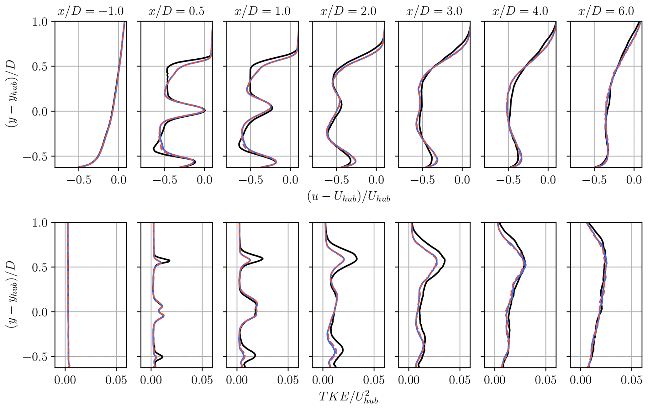
Figure 13 Profiles of mean velocity deficit (top) and turbulent kinetic energy (bottom) in the near wake of the turbine at various downstream locations: rigid undeformed (solid black line), rigid deformed (solid blue line), and flexible (dashed red line) cases.

First, the wake statistics are considered. The statistics are computed over the last 150 rotations to ensure that the wake is developed up to the end of the computational domain before averaging. The discarded first 50 rotations correspond to approximately 1.5 flow-through times, which was verified to be sufficient to reach a statistically converged flow. The averaging window of 150 rotations then corresponds to approximately 4.4 flow-through times. Figure 13 illustrates the time-averaged velocity deficit and turbulent kinetic energy (TKE) profiles. The differences between the profiles of the mean velocity deficit are comparable to the changes in the mean load distribution, which are the main source of differences between the wakes. Behind the tip of the turbine, the deficit is more pronounced in the rigid undeformed case compared to the deformed and flexible cases. Additionally, there is a steeper gradient of mean velocity behind the tip in this case. The TKE is also noticeably higher in the near-tip region, which results in a faster turbulent diffusion of the wake. For the rigid undeformed case, the velocity deficit observed 3 and 4 D behind the turbine is smaller but more diffuse than in the deformed cases. In the far wake (6 D behind the rotor), the velocity deficit and TKE profiles are almost equivalent. The time-averaged velocity deficit and TKE are very similar between the rigid deformed and flexible cases, which indicates that the unsteady variations around the mean deformation have a limited effect on the time-averaged wake statistics.

Some differences between the near wake of the rigid deformed and flexible cases can nevertheless still be observed. Figure 14 presents the difference in the mean velocity and TKE over vertical planes behind the rotor. The difference in the mean velocity behind the rotor ($x/D=\mathrm{0.5}$) is very close to that observed for the blade normal forces on the rotor area (see Fig. 10). The small changes in the local thrust result in differences in the mean velocity deficit that reach up to 2.5 % of the upstream velocity. The most substantial difference occurs behind the bottom of the rotor, where the velocity is significantly higher behind the rigid deformed turbine than behind the flexible turbine. Noticeable differences also exist behind the left and right parts of the rotor. At a distance $x/D=\mathrm{2}$, these differences start to vanish due to the wake destabilization that increases the turbulent mixing. The TKE exhibits a different behaviour, as it is globally lower in the rigid deformed case compared to the flexible case. The largest differences are observed for θ=90° and 270°, which also correspond to the angle with the highest variance of flapwise and torsional displacements. The increase in the TKE in the flexible case is attributed to the unsteady variations in the loads and position that further contribute to the fluctuations in the flow. However, these fluctuations remain moderate compared to the incoming turbulence of the wind and therefore have a limited impact on the wake behaviour.

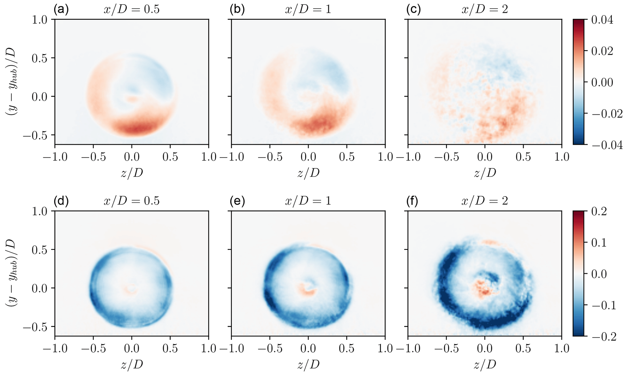
Figure 14 Difference in the mean velocity field (a, b, c, $(u_{\mathrm{r}.\mathrm{def}}-u_{\mathrm{flex}})/U_{\mathrm{hub}}$) and TKE (d, e, f, $({\text{TKE}}_{\mathrm{r}.\mathrm{def}}-{\text{TKE}}_{\mathrm{flex}})/{\text{TKE}}_{\mathrm{hub}}$) between the rigid deformed and the flexible cases over vertical planes at several locations behind the rotor.

A snapshot of an instantaneous out-of-plane vorticity field behind the rotor is depicted in Fig. 15 on a vertical plane. We stress that the turbulent inflow (provided by the co-simulation of the ABL) is at exactly the same time t for the three cases (i.e. it is synchronized), which allows us to compare fine details in the wake. The magnitude of the tip vortices behind the rigid rotors is significantly higher for the rigid undeformed rotor. This results from the higher gradient of the forces observed in the near-tip region for the undeformed blades. Additionally, these tip vortices are emitted further upstream compared to those of the deformed cases. As a result, the destabilization of the wake occurs at a smaller distance from the rotor. The rigid deformed and the flexible cases exhibit very similar vortical structures, even in the finer details. The wakes are almost identical, which further confirms the minimal influence of the unsteady fluctuations in the blade deformations on their mean deformation.

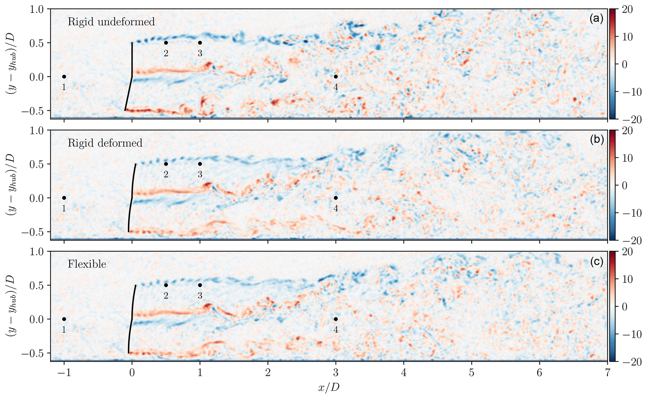
Figure 15 Snapshot of an instantaneous out-of-plane vorticity field (${\mathit{\omega }}_{z}D/U_{\mathrm{hub}}$) in the wake of the turbine for the rigid undeformed (a), rigid deformed (b), and flexible (c) cases. The inflow is identical for each case. The locations of the probes used for the velocity spectra are also shown.

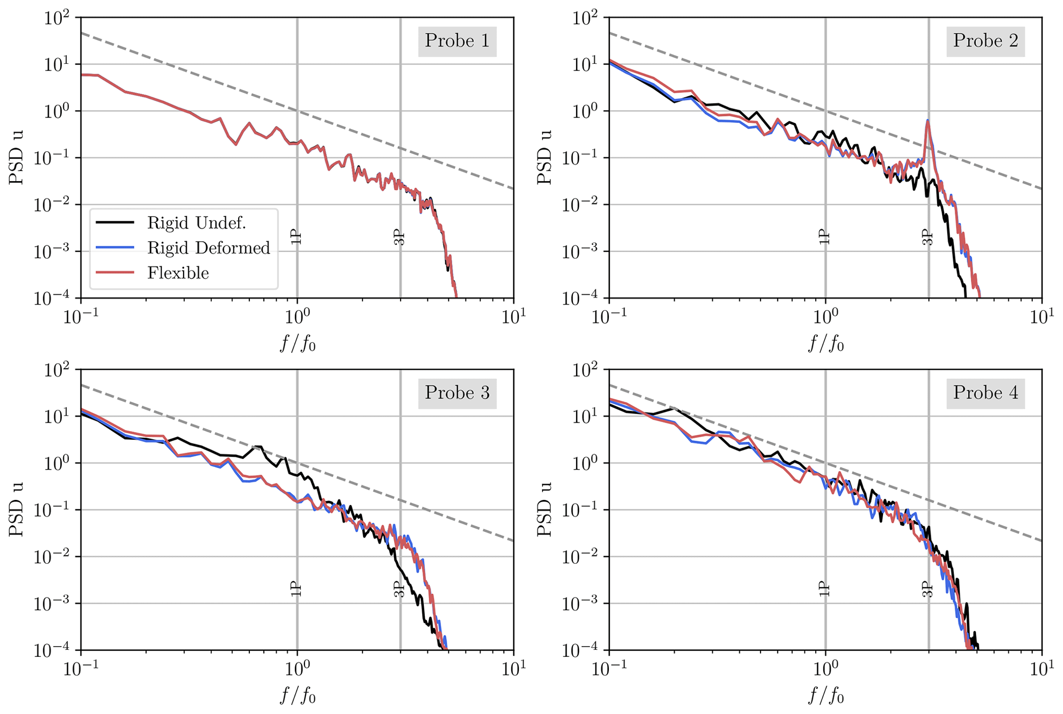
Figure 16 PSD of the streamwise velocity at various locations (as depicted in Fig. 15). The dashed line indicates the $(f/f_{\mathrm{0}}{)}^{-\mathrm{5}/\mathrm{3}}$ function.

The streamwise velocity is measured at various locations in the wake for each case to compare the flow statistics. Four locations are selected, as depicted in Fig. 15. The power spectral density of the streamwise velocity (obtained using the Welch algorithm) is then depicted for each case in Fig. 16. The first location is 1 D upstream of the hub in the induction zone (Probe 1), and the three PSDs are virtually identical, which confirms that the differences in the downstream flow can be fully attributed to the changes in the turbine aerodynamics. The flow velocity is also sampled behind the blade tip at two positions. In the very near wake (0.5 D behind the rotor, Probe 2), the blade passing frequency is clearly noticeable for the deformed and flexible cases, whereas it is not visible in the rigid undeformed case. This can be related to the fact that the tip vortices are well separated at this location in the deformed and flexible cases, while they already merged into a vortex sheet in the rigid undeformed case. Additional differences can be observed further in the wake (1 D behind the rotor, Probe 3), where the rigid undeformed case presents a much higher PSD at the frequencies lower than 1P. This increase is due to the destabilization of the vortex sheet, which results in lower-frequency velocity variations. In contrast, the rigid deformed and flexible cases do not exhibit such an increase, indicating that the wake remains stable at this location. Finally, the velocity is measured further downstream, 3 D behind the hub (Probe 4), where the influence of the hub vortices is minimal. At this location, the three PSDs are similar. For each location, the differences between the rigid deformed and the flexible case are small, confirming the limited impact of the unsteady variations on the wake.

The wake recovery rate is measured for each case by computing the power available in the flow P_w on the rotor-swept area A_rot. The latter is obtained as a function of the streamwise coordinate x as

$$\begin{array}{}\text{(3)}& P_{\mathrm{w}}\left(x\right)={\displaystyle \frac{\mathrm{1}}{\mathrm{2}}}\mathit{\rho }\underset{A_{\mathrm{rot}}}{\iint }{\stackrel{\mathrm{‾}}{u}}^{\mathrm{3}}(x,y,z)\mathrm{d}y\mathrm{d}z.\end{array}$$

The variation in the power (normalized by the power P₀ at the inflow) is depicted in Fig. 17. The available power in the wake of the rigid undeformed case is lower in the near wake due to the higher thrust coefficient. It also presents a faster recovery rate since it reaches the same level as the two other cases for $\mathrm{2}<x/D<\mathrm{6}$. However, in the far wake, it is also slightly lower than in the rigid deformed and flexible cases. These two cases again present almost identical statistics.

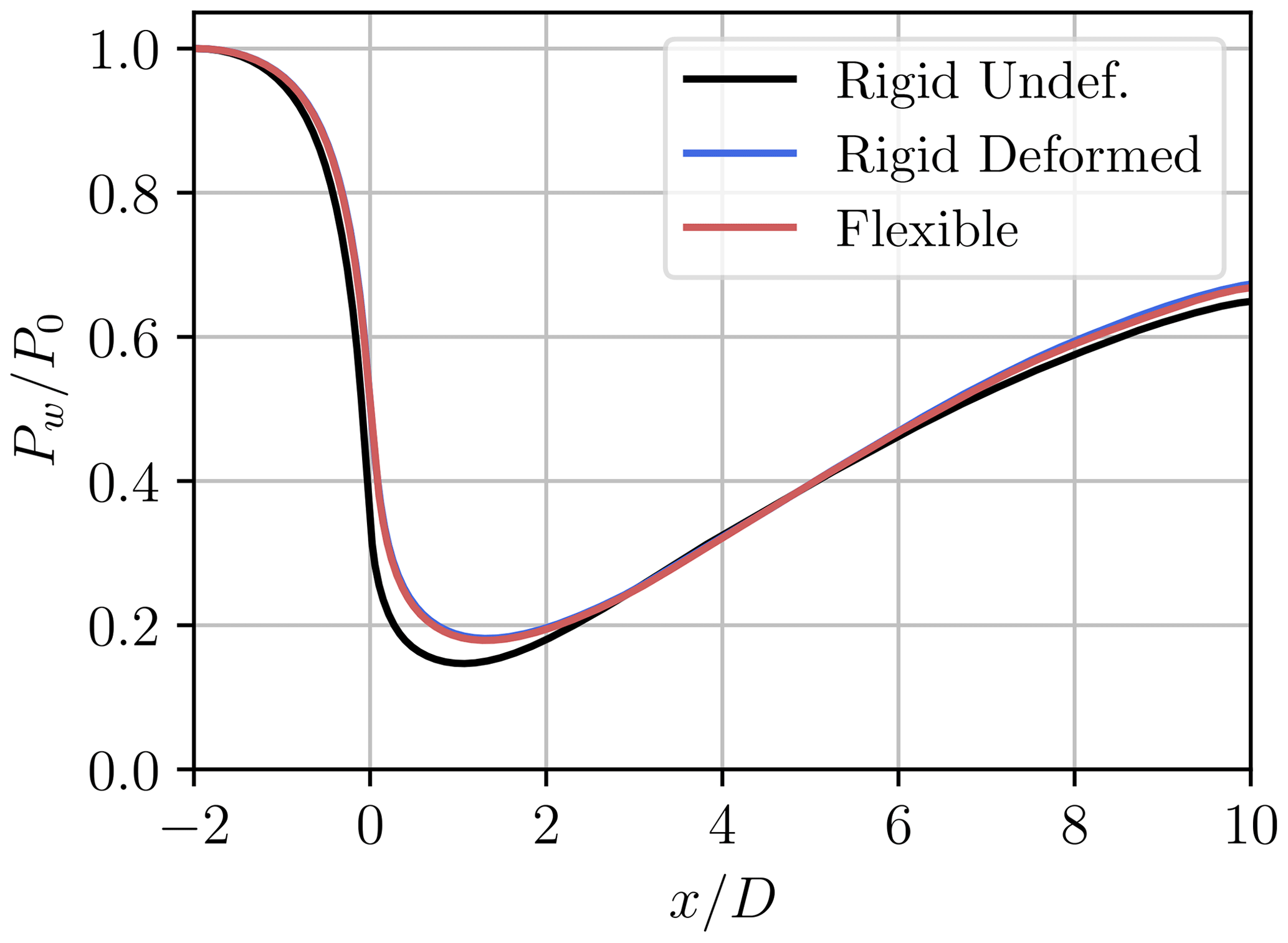
Figure 17 Available power in the wake (normalized by the power at the inflow), computed over the rotor-swept area at various streamwise locations.

This analysis shows the necessity of including the mean deformation to accurately capture the near wake but also predicts a minimal effect of the unsteady variations of the displacements and loads around their mean. The spatial resolution of the presented simulations is 64 points per D, corresponding to 3.75 m, which is larger than the variation in the displacements along the mean deformed configuration. To further assess the impact of the small variations, it is important to verify that the resolution of the flow simulations is sufficient. The next section therefore assesses the effect of the spatial resolution on the loads and near-wake dynamics.

Figure 18 Distribution of the aerodynamic loads along the blade span for the initial resolution (grey line) and the increased resolution (red line). The shaded area represents the standard deviation. (a) Flapwise forces; (b) edgewise forces.

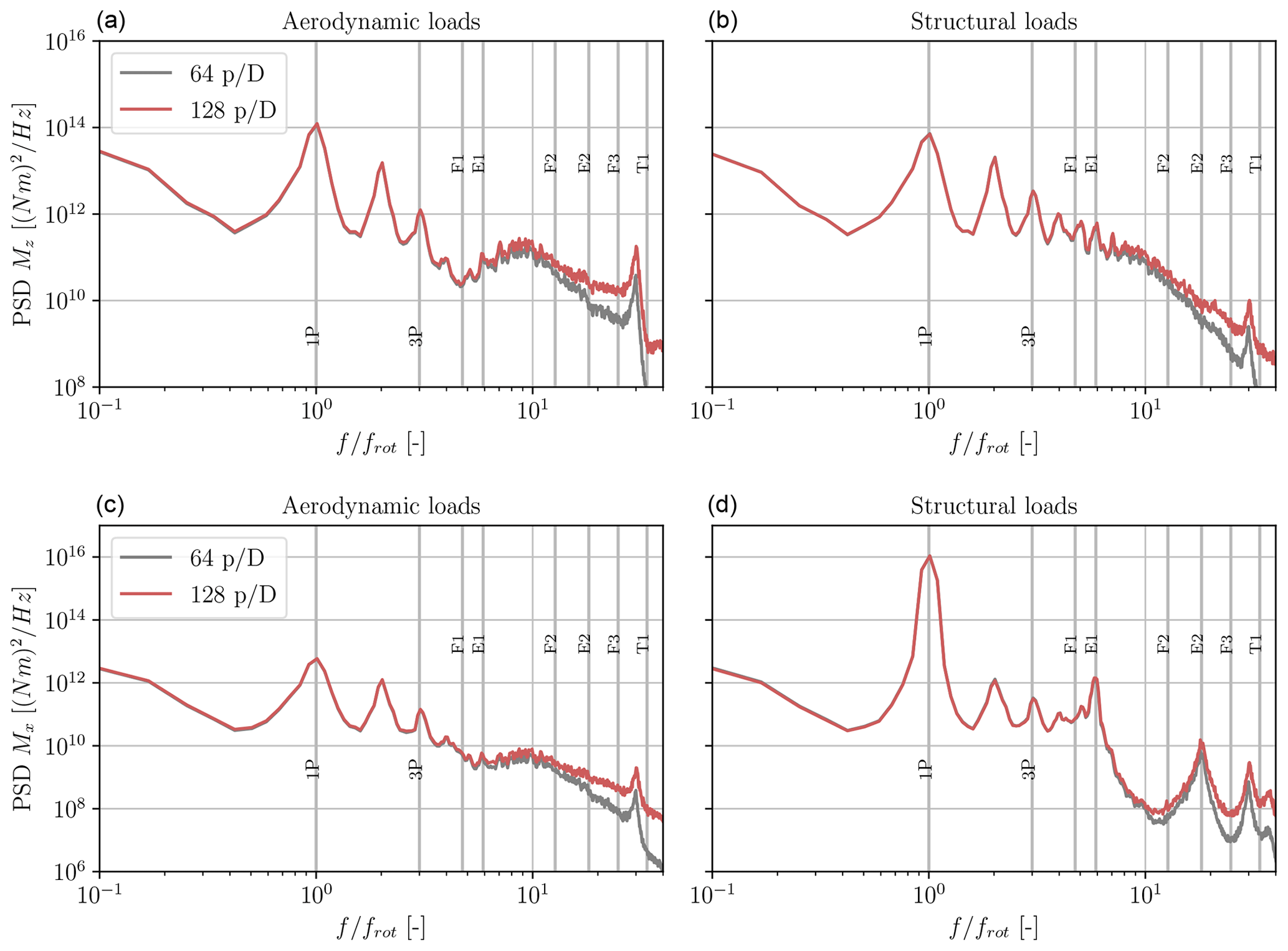
Figure 19 PSD of the blade root moment due to the flapwise forces (M_x, a, b) and edgewise forces (M_z, c, d). (a, c) PSD of the moment of the aerodynamic loads; (b, d) PSD of the structural root moment. Comparison between two resolutions: 64 points per D (grey line) and 128 points per D (red line).

5 Investigation of the impact of the spatial resolution

In this section, the results obtained with a spatial resolution of 64 grid points per diameter are compared to those of a higher-resolution simulation to assess whether the small deviations in loads and displacement around the mean are sufficiently resolved. The case of a flexible rotor is therefore reconsidered with a grid resolution twice as fine, corresponding to 128 grid points per D. The time step is also divided by 2 to maintain the Courant–Friedrichs–Lewy (CFL) number constant. The mollification of the ALM forces is kept constant relative to the grid size (i.e. $\mathit{\sigma }/h=\mathrm{2}$) and is thus 2 times smaller for the highest resolution. The resolution of the precursor simulation is similarly increased, and the smaller scales of the turbulence are obtained by restarting the ABL simulation at the new resolution and converging it during ≃25 flow-through times. The simulation with the resolution of 64 points per D is also performed using the same precursor simulation, which is interpolated to the coarser resolution at the inflow plane. This ensures a valid comparison between the two simulations.

The mean force distribution on the blades is depicted for both resolutions in Fig. 18. The two distributions and their variances are very close. The thrust coefficient C_T is 0.687 for the simulation with 64 points per D, and it increases slightly to 0.692 for 128 points per D (+0.7 %). Similarly, the power coefficient increases from 0.439 to 0.445 (+1.3 %). The general shape of the distribution remains consistent between the two simulations, also near the tip, which suggests a sufficient discretization of the blade and the wake.

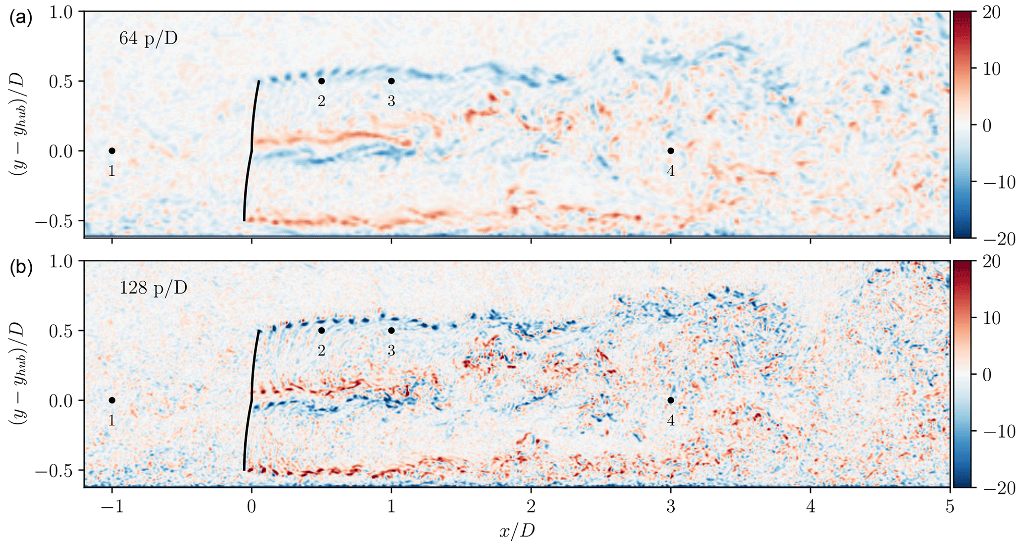
Figure 20 Snapshot of an instantaneous out-of-plane vorticity field (${\mathit{\omega }}_{z}D/U_{\mathrm{hub}}$) in the wake of the turbine for the 64 points per D resolution (a) and the 128 points per D resolution (b) cases. The inflow is identical for each case. The locations of the probes used for the velocity spectra are also shown.

The variations in the aerodynamic forces and structural root moment are also depicted in Fig. 19. The presented PSDs match perfectly until the E1 frequency. For higher frequencies, the loads predicted using 128 points per D are higher. This is due to the additional unsteadiness induced by the smaller turbulent scales that are resolved up to a higher frequency when at high resolution and the smaller mollification size that reduces the smoothing induced by the integral velocity sampling. The magnitude of the PSD at these high frequencies is however much lower than that of the small frequencies; hence it is unlikely that this additional part of the spectrum significantly affects the fatigue of the blades and the wake. The peaks of the PSD located at the E2 and T1 frequencies are also obtained in both cases, indicating that the main components of the structural response are not significantly impacted by the resolution.

Figure 20 presents the instantaneous vorticity field behind the rotor with the two resolutions. The same velocity fields obtained at a resolution of 128 points per D and at the same time t are used at the inflow of both simulations. The only difference is that the inflow is interpolated from 128 to 64 points per D at the inflow plane of the coarser simulation. At higher resolution, the tip vortices have a smaller core size and hence a higher vorticity at their centre (since they essentially have the same circulation in both cases). The hub vortices are also better resolved. The shed vortex sheet behind the outer part of the blade is also distinguishable. However, the larger structures of the wake are similar in both cases. This results in virtually identical velocity deficits as depicted in Fig. 21. The TKE has a higher value behind the hub and in the near-tip regions, which results from the sharper mollification and the smaller scales captured by the simulation. However, this does not affect the mean velocity deficit.

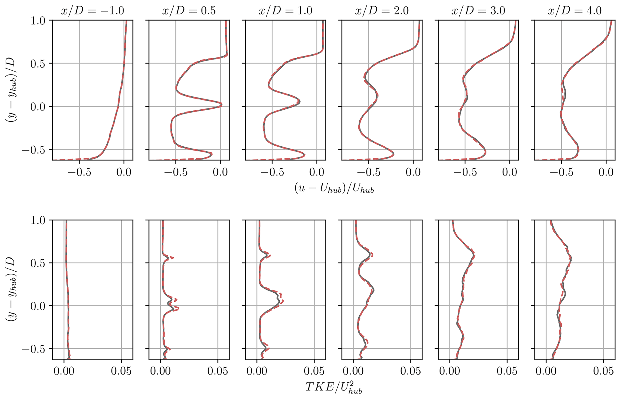
Figure 21 Profiles of mean velocity deficit (top) and turbulent kinetic energy (bottom) in the near wake of the turbine at various downstream locations. Comparison between the 64 points per D (grey line) and 128 points per D (dashed red line) resolutions.

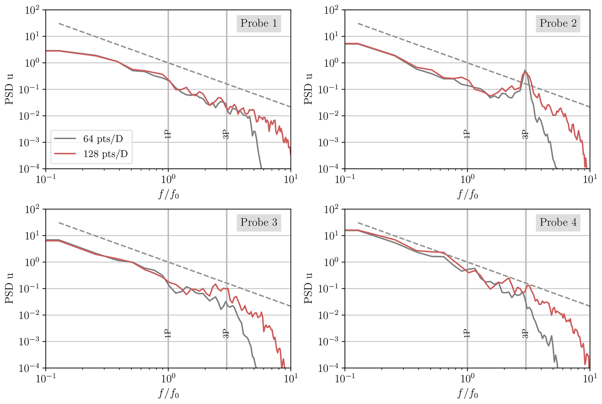
Figure 22 PSD of the streamwise velocity at various locations (as depicted in Fig. 20). Comparison between the 64 points per D (grey line) and 128 points per D (red line) resolutions.

The PSD of the streamwise velocity at various locations in the domain is also compared for both resolutions. The locations where the flow velocity is sampled are depicted in Fig. 20, and the obtained spectra are shown in Fig. 22. The first spectra are obtained using the streamwise velocity measured 1D upstream of the hub (Probe 1). At this location, the PSD obtained for the simulation with 64 points per D decreases much faster at higher frequencies, as expected from the smaller LES cut-off frequency. There are also some slight differences below the cut-off frequency due to the interpolation at the inflow from the ABL with 128 points per D resolution to the LES with 64 points per D resolution and the variation occurring during the convection of the turbulence between the inflow and the sampling location. In the near wake, the PSD of the velocity measured 0.5 D behind the blade tip (Probe 2) is very similar between the two resolutions (except at the highest frequencies). When measuring 1 D downstream of the blade tip (Probe 3), the peak of the PSD obtained for the simulation with 128 points per D is more pronounced near the 3P frequency due to the more distinct tip vortices, whereas the tip vortices have merged into a vortex sheet in the simulation with 64 points per D. Further in the wake, 3 D behind the hub (Probe 4), the spectra are in good agreement at the lower frequencies and only show deviations at the higher frequencies.

6 Conclusions

This work presented an investigation of the effect of the flexibility of the blades on the loads and the wake for the large IEA 15 MW reference wind turbine. A flexible actuator line method (ALM), coupled to the nonlinear structural solver BeamDyn, is used in large-eddy simulations (LES) to compute the unsteady aerodynamic forces exerted by the turbulent inflow on each blade and their influence on the flow. This methodology leverages the LES capabilities to realistically simulate the unsteadiness of the inflow and the wake produced by the turbine in order to quantify the effect of the structural blade deformations on the loads and the wake.

The results obtained using the flexible actuator line method are first compared to those obtained using OpenFAST. In uniform flow, the free vortex wake model of OpenFAST and the present flexible ALM predict very similar distributions for the forces, which are slightly higher than those predicted using a BEM in the tangential direction. The effect of the deformation of the blades on the time-averaged loads is also predicted similarly by OLAF and the ALM. The magnitude of this effect is larger than that predicted by the BEM, which indicates that higher-fidelity aerodynamic models are necessary to account for the effect of large displacements on the blade aerodynamics. Comparisons carried out using a turbulent inflow without mean shear (generated using the Mann algorithm) show that the power spectral densities (PSDs) of the blade displacements are very similar for all three methods, which confirms that the flexible actuator line model is able to correctly capture the structural dynamics.

The displacement and loads of the blades are then investigated in a turbulent atmospheric boundary layer (generated using a co-simulation). Notable flapwise and torsional displacements are observed, which significantly modify the aerodynamics of the blades. The resulting thrust coefficient decreases by 14 % and the power coefficient by 10 % compared to the rigid undeformed case. Including the mean deformation while keeping the rotor rigid allows us to correctly recover the mean load distribution along the blade, which leads to thrust and power coefficients equivalent to those obtained using the flexible actuator line method. However, the variation in the loads during the blade rotation is different, especially close to the blade's downward position, due to the high mean shear of the flow. Moreover, the aerodynamic loads and the structural response at the blade natural frequencies are noticeably affected by the flexibility. We also show that the variation in the angle of attack due to the flapwise blade velocity is significant and of the same order of magnitude as that due to the blade torsion.

The wake behind the turbine is then considered. The results show that it is essential to include the mean deformation of the blade to obtain the correct mean velocity deficit and profile of turbulent kinetic energy. Once the mean deformation is added, the differences between the rigid deformed and the flexible cases are limited. In the near wake, the time-averaged velocity obtained in the flexible case is up to 4 % slower at the bottom of the rotor-swept area than in the rigid deformed case. The turbulent kinetic energy is slightly higher over the rotor area, which results from the unsteady variations in the loads and displacements. However, these changes do not significantly affect the global wake behaviour.

Finally, the effect of the LES flow solver resolution on the wake is investigated by increasing the spatial discretization to 128 grid points per diameter. The mean load distribution is comparable to that obtained using the resolution with 64 grid points per diameter. The PSD of the root moment is also identical up to the first edgewise frequency. For the higher frequencies, a difference in magnitude is observed due to the higher-frequency fluctuations captured by the LES (due to the twice higher cut-off wavenumber of the grid). A snapshot of the wake vorticity field shows tip vortices with a smaller core size, and hence a higher vorticity at their centre, and smaller turbulent scales in the flow. However, the time-averaged velocity deficits are largely similar between the two simulations. The TKE is higher behind the blade root and tip at high resolution, yet this does not impact the turbulent wake diffusion rate. As a result, it is unlikely that a higher resolution would significantly increase the impact of the unsteady displacements and load variations on the wake. It would however be necessary if the spectrum of the loads must be obtained at high frequencies.

The impact of the structural deformations on the loads and wake of a large 15 MW turbine is thus significant. These effects consist of a reduction in the thrust and power coefficients, a variation in the load distribution over the blade, and a modification of the spectrum of the blade root moments. These changes, in turn, substantially affect the near wake by altering the profiles of the velocity deficit and turbulent kinetic energy. In the relatively steady operating conditions considered in this paper (i.e. constant time-averaged wind velocity, turbulence intensity, and rotation speed), the proper mean load distribution and wake behaviour can be obtained using rigid blades but only when adjusting their geometry to incorporate their mean structural deformation. Here, the latter was obtained by time averaging the structural deformation produced by our fully coupled unsteady simulations, but it could also be obtained in a preprocessing step, using alternative aeroelastic simulation tools. This then removes the need for the unsteady coupling of the structural solver and the actuator line of the LES solver, thereby reducing the computational cost slightly. However, the unsteady variations in the mean would still differ compared to those of the fully coupled simulation, resulting in a different spectrum of the loads. It is hence recommended to include the structural dynamics of the blades if the unsteady variation in the loads is of interest, particularly for a blade structural integrity assessment or to assess the benefits of load alleviation control methods.

Appendix A: Parallel implementation of the ALM and structural solver

Figure A1 Schematic of the structural coupling.

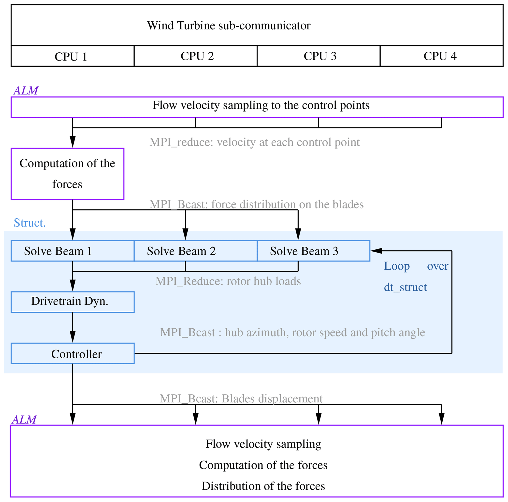
The following Appendix describes in more detail the strategy employed for parallelizing the computations related to the ALM and the structural solver. A separate subcommunicator is defined for each wind turbine, which is split from the main communicator based on the turbine location. Any process containing a grid point closer to the hub than a distance D is included in the turbine communicator. As the subcommunicators of each turbine generally comprise a distinct set of processors, the tasks related to the ALM and the structural solver can be performed concurrently for each turbine. The different steps performed on the local set of processes are shown in Fig. A1. The subcommunicator is first used to sample the velocity within a restricted region of the physical domain, thereby decreasing the communication overhead. The aerodynamic forces are computed on the root processor using the sampled velocities. Subsequently, the forces are broadcasted to the structural solver, which executes one instance of BeamDyn per blade on different processors. The time integration of the blade dynamics is therefore performed in parallel, and the resulting root moments of each blade are sent to the root process. The latter computes the drivetrain dynamics and the controller commands at each structural sub-step. The beam solver only takes the hub azimuth and the pitch angle (and their time derivatives) as input and only needs to provide the forces and moments on the hub as output. Consequently, the overhead of the added communications required to solve the blade dynamics in parallel is largely overcome by the benefits of the parallelization. After completion of the sub-steps, the blade displacements are broadcasted to all the processors of the subcommunicator to be used for the re-evaluation of the forces and their distribution. The following parallelization allows us to keep the computational cost of the ALM and its coupling to BeamDyn reasonably low and provide an efficient scaling in the case of multiple turbines.

Appendix B: Statistics of the simulated atmospheric boundary layer

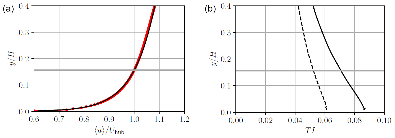
Figure B1 (a) Profile of the obtained mean streamwise velocity (dotted red line) and its comparison to a logarithmic profile (solid black line). (b) Profile of the turbulence intensity based on the streamwise velocity (solid line) and the three velocity components (dashed line). The horizontal grey line indicates the hub height.

This section presents the statistics of the neutral ABL that is used as inflow for the wind turbines. It is obtained by simulating a turbulent half-channel flow of height H=4 D; hence H=960 m. The flow is driven using a pressure gradient $(-\mathrm{d}p/\mathrm{d}x)/\mathit{\rho }=\mathrm{1.148}\times {\mathrm{10}}^{-\mathrm{4}}$ m s⁻² (with ρ=1.225 kg m⁻³ for air). The lateral boundary conditions are periodic. The upper boundary condition is a no-slip condition. At the ground, a wall model is used. The latter imposes the shear stress at the wall using the law of the wall for a rough wall,

$$\begin{array}{}\text{(B1)}& u\left(y\right)={\displaystyle \frac{u_{\mathit{\tau }}}{\mathit{\kappa }}}\log \left({\displaystyle \frac{y}{y_{\mathrm{0}}}}\right),\end{array}$$

with κ=0.385 and y₀=0.0016 m. The computational domain is $\mathrm{8}D\times \mathrm{4}D\times \mathrm{4}D$ and is discretized using a uniform structured mesh with a resolution of 64 grid points per D. The time step is set to dt=0.05 s, and the simulation is run for 584 flow-through times $t^{*}=t{U}_{\text{hub}}/\left(\mathrm{8}D\right)$ before it reaches convergence. The following statistics are then computed over ≃100 flow-through times.

The obtained profiles of the mean streamwise velocity and the turbulence intensity are shown in Fig. B1. The mean velocity profile indeed corresponds to a logarithmic profile with u_τ=0.332 m s⁻¹, and the turbulence intensity decreases linearly with height. The mean velocity of 10 m s⁻¹ is obtained at the hub, as well as a TI of ≃5 % when computed using the three velocity components. There are some small oscillations in the TI near the ground resulting from the large gradients at the wall. However, these oscillations are located at the bottom of the domain and do not affect the rotor region. The auto-correlation functions of the streamwise velocity, ${\mathit{\rho }}_{u,u}^x$ and ${\mathit{\rho }}_{u,u}^z$, in the streamwise and lateral directions, respectively, are also depicted in Fig. B2. These are used to compute the integral length scale in the streamwise and lateral directions, $L_u^x$ and $L_u^z$, obtained by integration (Stanislawski et al., 2023):

$$\begin{array}{}\text{(B2)}& L_u=\underset{\mathrm{0}}{\overset{\widehat{\mathit{\delta }}}{\int }}\langle {\mathit{\rho }}_{u,u}\left(\mathit{\delta }\right)\rangle d\mathit{\delta },\end{array}$$

where $\widehat{\mathit{\delta }}$ is the distance where the correlation function is smaller than 0.05. This leads to $L_u^x$ = 106 m = 0.44 D and $L_u^z$ = 89.5 m = 0.37D.

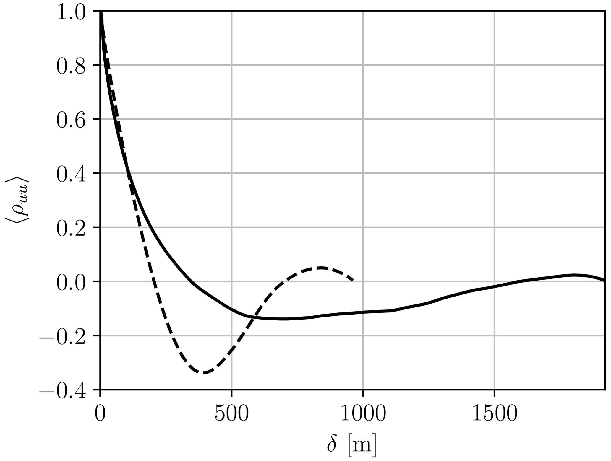
Figure B2 Auto-correlation functions of the streamwise velocity in the streamwise ($\langle {\mathit{\rho }}_{uu}^x\rangle$, solid line) and lateral ($\langle {\mathit{\rho }}_{uu}^z\rangle$, dashed line) directions. The values are averaged over the horizontal plane at hub height.