the Creative Commons Attribution 4.0 License.
the Creative Commons Attribution 4.0 License.
 | 29 Jan 2024
The wind farm pressure field
Ronald B. Smith
The disturbed atmospheric pressure near a wind farm arises from the turbine drag forces in combination with vertical confinement associated with atmospheric stability. These pressure gradients slow the wind upstream, deflect the air laterally, weaken the flow deceleration over the farm, and modify the farm wake recovery. Here, we describe the airflow and pressure disturbance near a wind farm under typical stability conditions and, alternatively, with the simplifying assumption of a rigid lid. The rigid lid case clarifies the cause of the pressure disturbance and its close relationship to wind farm drag.
The key to understanding the rigid lid model is the proof that the pressure field p(x,y) is a harmonic function almost everywhere. It follows that the maximum and minimum pressure occur at the front and back edge of the farm. Over the farm, the favorable pressure gradient is constant and significantly offsets the turbine drag. Upwind and downwind of the farm, the pressure field is a dipole given by , where the coefficient A is proportional to the total farm drag. Two derivations of this law are given. Field measurements of pressure can be used to find the coefficient A and thus to estimate total farm drag.
- Article
(2825 KB) - Full-text XML
- BibTeX
- EndNote


The construction of offshore wind farms may significantly help our society transition to renewable energy, but the wind slowing by these farms may ultimately limit their potential for electric power generation (Ahktar et al., 2022). This issue has an extensive literature, reviewed recently by Stevens and Meneveau (2017), Archer et al. (2018), Porte-Agel et al. (2020), Pryor et al. (2020), and Fischereit et al. (2021). An integral part of the wind slowing by turbine drag is the creation of a local pressure field. This pressure disturbance was initially neglected (Jensen, 1983) but has been recently estimated in connection with gravity wave (GW) generation (Smith, 2010, 2022; Wu and Porté-Agel, 2017; Allaerts and Meyers, 2018, 2019). In a stably stratified atmosphere, the lifting of the air caused by farm drag creates gravity waves aloft whose pressure field acts back on the lower atmosphere.
This pressure field modifies the airflow in ways that the direct action of turbine drag cannot. First, it can decelerate the flow before it reaches the first row of turbines, so-called “blockage” (Bleeg et al., 2018) in wind farm terminology or “blocking” in mountain meteorology. Second, it can deflect the air to the left and right. Third, over the farm, it can fight back against the turbine drag, helping to keep the wind flow strong. Finally, it slows the downwind recovery of the wake.
The pressure field near a wind farm is analogous in some respects to that for a single turbine. The airflow approaching a turbine disk begins to decelerate upwind due to an adverse pressure gradient, and its corresponding axial induction factor reduces the turbine efficiency to the Betz limit (Hanson, 2000). According to Gribben and Hawkes (2019), the local non-hydrostatic pressure disturbance decays inversely as the square of the distance upstream. The farm-generated hydrostatic pressure disturbance may be more far-reaching.
In discussing the cause of the pressure field, we shall exercise caution as the cause may be model dependent. In compressible subsonic aerodynamics, acoustic waves play a role in creating the pressure field. In stratified flow, gravity waves play a role. In presumed non-divergent flow, the pressure field is usually determined diagnostically as the cause is hidden from view. The pressure field exists simply to keep the flow non-divergent.
In this paper, we compare the wind farm pressure field in the realistic gravity wave (GW) model with the idealized rigid lid (RL) model. The rigid lid approximation retains some of the features of the atmospheric problem but allows us to derive simple theorems and closed-form solutions that clarify the cause, nature, and impact of the pressure field.
We begin by recalling the governing equations for the two-layer model of Smith (2010) and describe the rigid lid (RL) limit. Second, we derive approximate closed-form expressions for the far-field and near-field pressure. Third, we discuss the cause of the pressure field and its role in the wind farm disturbance. Finally, we consider using pressure measurements to estimate total farm drag and the use of the RL model in industrial applications.
Our method for computing the response to wind farm drag forces uses a two-layer stratified hydrostatic gravity wave (GW) model solved with fast Fourier transforms (FFTs). This model consists of a lower turbine layer from which momentum is removed by specified drag forces and a Rayleigh restoring force that decays the farm wake (Smith, 2010, 2022). An overlying density-stratified layer responds to vertical displacement and creates a hydrostatic pressure field p(x,y) that acts back on the turbine layer. The linearized governing momentum equations for the turbine layer are
where F(x,y) is the turbine drag, U is the ambient wind, u(x,y) is the drag-induced perturbation wind, and C is the Rayleigh restoring coefficient (Smith, 2022). After these equations are solved for the perturbation wind field, the linearized scalar wind deficit is computed from . Its area integral is the total deficit:
Taking the dot product of Eq. (1) with the ambient wind and integrating over the whole domain relates TD to the turbine drag (Smith, 2022):
Because the pressure field p(x,y) decays at infinity, it does not influence TD but alters the spatial distribution of Deficit(x,y). The impact of the deficit on farm power generation is described by the average relative speed deficit . For example, γ=0.02 is a 2 % reduction in wind speed over the farm.
The GW model discussed herein uses the hydrostatic assumption and thus does not take into account the pressure field associated with vertical fluid acceleration. Pressure fields in this model are generated only by density anomalies aloft. If an airflow streamline approaching a wind farm curves sharply upwards, a region of non-hydrostatic high pressure will be generated below it. These effects are easily incorporated in the linearized FFT modeling framework, but we do not do that here. In mountain wave theory, for example, such effects are usually neglected for horizontal scales greater than 1 km. Non-hydrostatic effects are certainly important on the scale of an individual turbine but less so on the farm scale where hydrostatic effects are expected to dominate. Some wind farm models, such as that of Gribben and Hawkes (2019), include the non-hydrostatic effect but neglect the hydrostatic effect.
We first ran the two-layer GW model with the realistic parameters shown in Table 1. The model's two stability parameters are the reduced gravity g′ of the inversion and Brunt–Väisälä frequency N of the troposphere given by
where θ is the potential temperature. We set the Rayleigh restoring coefficient C to a fairly small value so the wake recovery is slow but fast enough to prevent periodic wrapping from the FFT method. To compute the turbine drag force F, we define the disk area ratio (DAR) as the ratio of rotor disk area to planform farm area. We chose DAR=0.0077 and a turbine thrust coefficient of CT=0.75. With a wind speed of U=10 m s−1 and turbine layer depth of H=400 m, the wind farm drag per unit air mass is then
For illustration, we chose horizontal farm dimensions m. The total drag on the farm is then
A few output parameters from this reference run are given in Table 2, including the maximum vertical displacement of the inversion, the maximum wind speed deficit, the normalized farm-averaged speed deficit (γ), and the difference between the two pressure extrema (Δp). In the reference run, the inversion is displaced upward by 11.8 m, the maximum speed deficit is 0.468 m s−1, the average relative speed deficit is γ=0.0315, and there is a Δp=2.38 Pa pressure difference across the farm.
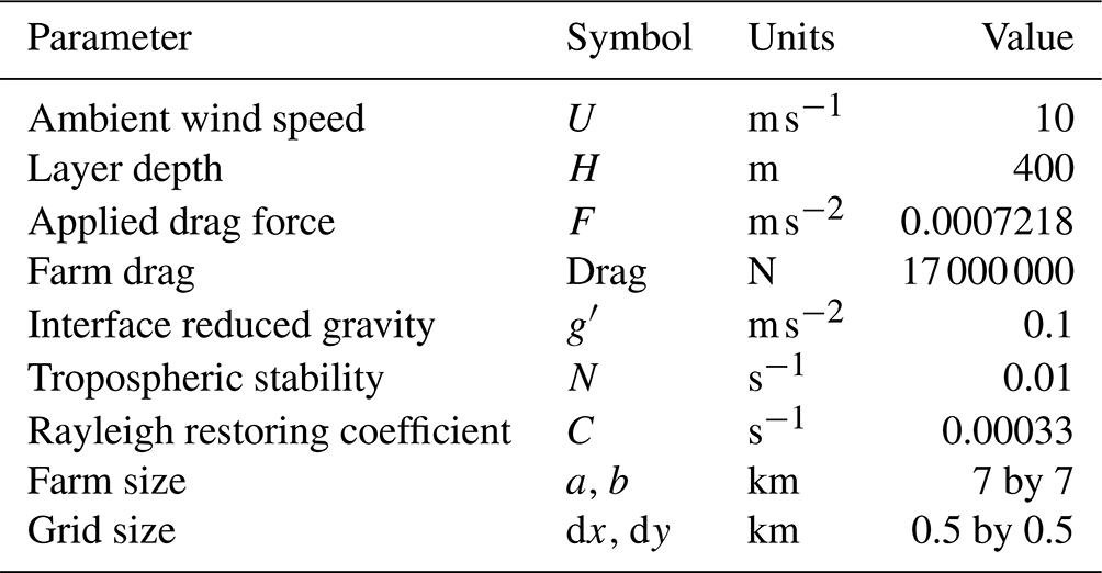
Table 2Wind farm disturbance properties as stability is increased towards the rigid lid limit. The value A is the estimated strength of the pressure dipole. Note that n/a stands for not applicable.
a Reference GW case. b Near-resonant case Fr≈1.
To investigate the influence of atmospheric stability (Eq. 4), we ran the GW model several more times – first with the two stability parameters . When there is no stability, the turbine drag slows the airstream and displaces the top of the turbine layer upwards, but no hydrostatic pressure disturbance is generated.
We then increased each stability parameter (Eq. 4) from zero towards a large value (Table 2). The vertical displacement of the fluid decreased towards zero and the pressure perturbations increased from zero. Other model output values changed only slightly. The maximum wind speed deficit decreased slightly from 0.445 to 0.323 m s−1 in the rigid lid limit. The average relative speed deficit over the farm decreased slightly from γ=0.0226 to 0.0195.
One striking aspect of Table 2 is that the g′ series and the N series of runs approach the same rigid lid (RL) limit. The trends are smooth for the N series but the g′ series of runs shows a singularity when the Froude number . Ultimately, increasing either type of stability takes us to the same rigid lid solution with finite wind deficit and pressure difference but a vanishing vertical displacement. When N=0, the vertical displacement approaches zero as , and when it approaches zero as .
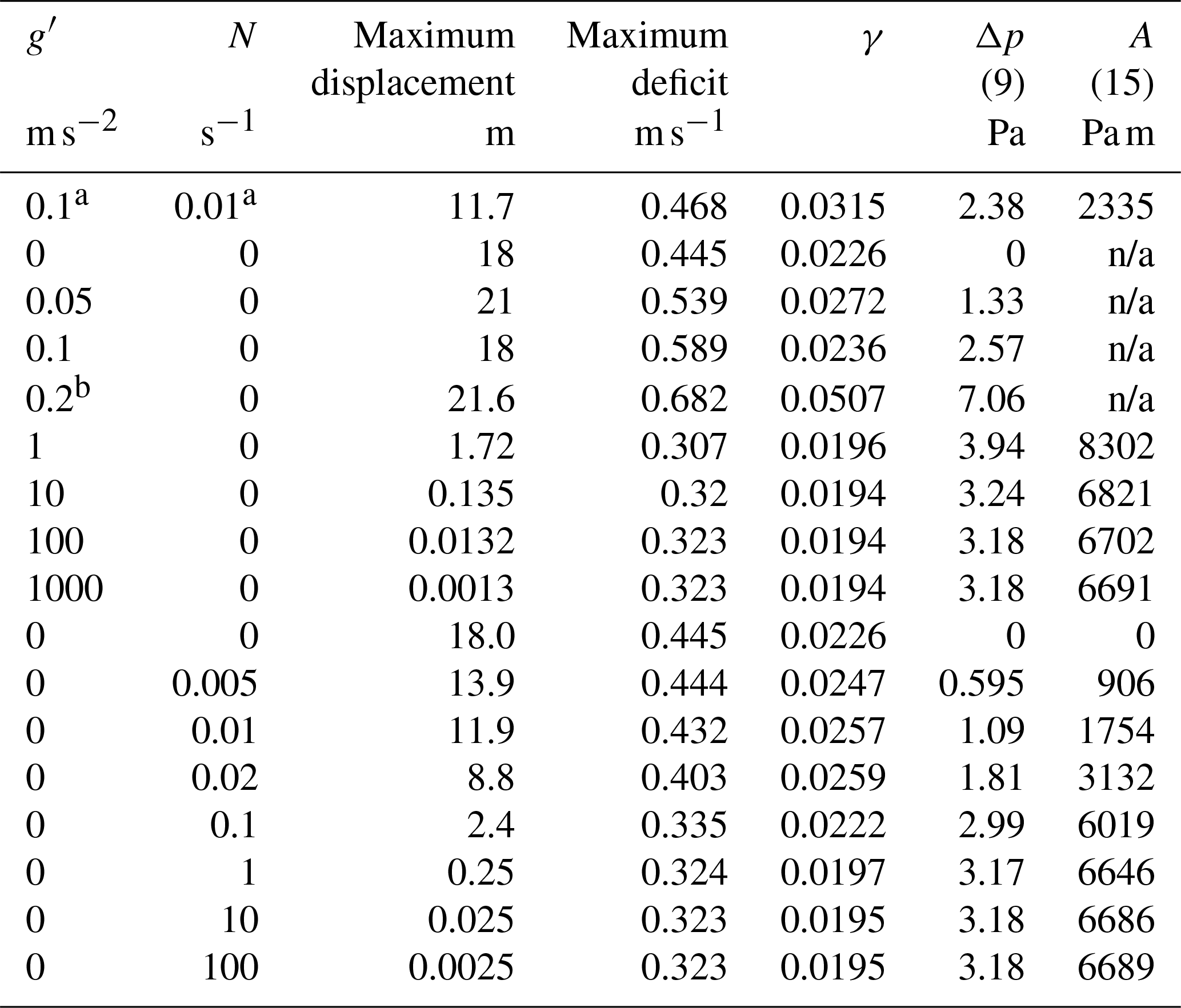
The planform patterns of the gravity wave (GW) and rigid lid (RL) solutions are compared in Figs. 1 and 2. The wind speed deficit patterns (Figs. 1a and 2a) show the wake caused by the farm drag but also show the influence of the pressure fields. Both show upstream deceleration, which is stronger in the RL case, and lateral regions of accelerated flow downwind of the farm. The wind speed deficit patterns over the farm are different also due to pressure forces acting on the flow. The pressure fields (Figs. 1b and 2b) show an upwind maxima and downwind minima of approximately similar magnitude. The RL case, however, has these two extrema shifted upwind, and the whole field is exactly anti-symmetric with respect to the upwind–downwind direction.
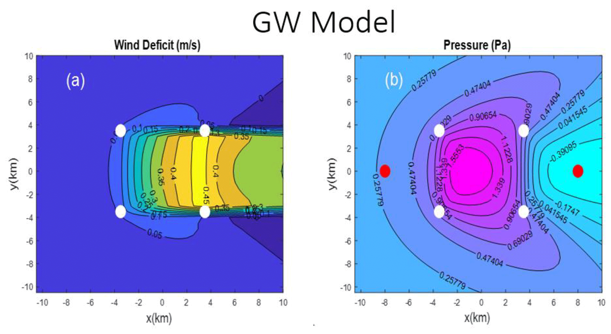
Figure 1Zoom of the disturbance caused by a 7 km by 7 km wind farm from the realistic gravity wave (GW) model: (a) wind speed deficit (m s−1) and (b) pressure (Pa). Airflow is from left to right. White dots mark the corners of the farm. In panel (b), the red dots are pressure sampling points. The full domain is 200 km by 200 km.
Figure 2Zoom of the disturbance caused by a 7 km by 7 km wind farm from the idealized rigid lid (RL) case: (a) wind speed deficit (m s−1) and (b) pressure (Pa). Airflow is from left to right. White dots mark the corners of the farm. In panel (b), the red dots are pressure sampling points. The full domain is 200 km by 200 km.
We can understand the rigid lid (RL) solution more fully by noting that the pressure field p(x,y) in that case is a harmonic function almost everywhere. A harmonic function is one which satisfies Laplace's equation ∇2p=0. To prove this hypothesis, we apply the divergence operator to Eq. (1), giving
With the rigid lid, the horizontal flow field is non-divergent flow so , and Eq. (7) becomes
Thus, the RL pressure field is a harmonic function except at the windward and leeward edges of the wind farm where the turbine drag force is divergent (i.e., ).
To illustrate the harmonic property of p(x,y) we show the Laplacian of the pressure field for the reference GW case in Fig. 3a and the rigid lid case in Fig. 3b. They differ in important details. In Fig. 3a, ∇2p=0 is violated over most of the field in a complicated pattern, while in Fig. 3b it is violated only over the farm front and back edges, in agreement with Eq. (8). The Laplacian in Fig. 3 was computed in Fourier space with and then inverted.
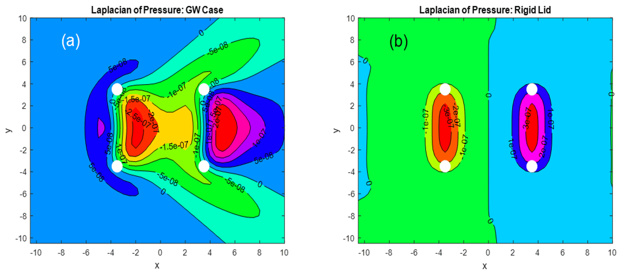
Figure 3Laplacian of the pressure field with units Pa m−2. (a) Reference GW case and (b) rigid lid case. Airflow is from left to right. White dots mark the corners of the farm. A low-pass filter has been applied to panel (b).
Recall that a harmonic function has no local maxima or minima and therefore only takes on values that are between the boundary values. As p(x,y) decays at infinity, the pressure would therefore vanish were it not for these two small non-harmonic regions. Thus, these two regions in Fig. 3b support or cause the pressure field seen in Fig. 2b.
In non-divergent flow, the role of pressure is to maintain the non-divergent property of the flow. As the turbine force field F(x,y) is divergent at the farm edges, the pressure field must arise instantly to prevent any flow divergence there. That is the meaning of Eq. (8). At the windward edge, for example, the outward diverging pressure forces balance the converging turbine drag forces.
This interpretation is supported by noting that pressure is insensitive to the Rayleigh restoring force coefficient C in Eq. (1). The dashed curve in Fig. 4b shows the wind speed deficit where we increase the coefficient 10-fold to C=0.0033 s−1. In Fig. 4b, the wind speed deficit is dramatically reduced while the pressure field is unchanged. This independence of the pressure field from C is a unique feature of the rigid lid case and not found in the more general GW case where the Rayleigh force is divergent. The Rayleigh force is non-divergent because the RL flow is non-divergent, and therefore it does not influence the pressure field.
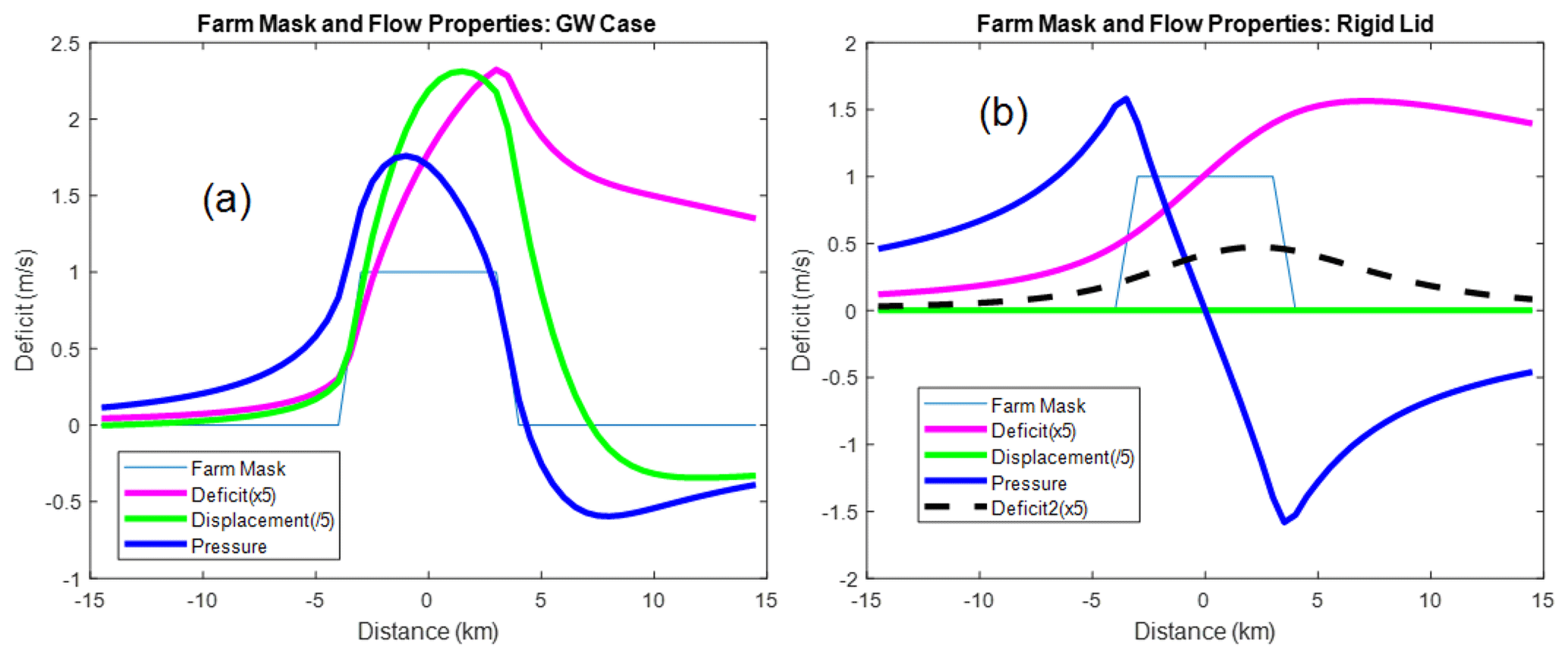
Figure 4Centerline properties of the farm disturbance including the farm mask, wind speed deficit (×5 m s−1), interface displacement ( m), and pressure (Pa): (a) reference GW case and (b) rigid lid case. In panel (b), the dashed line is the wind speed deficit with a larger Rayleigh restoring coefficient (C=0.0033 s−1). The pressure is unchanged. Airflow is from left to right.
The two pressure fields, GW and RL, are compared along the centerline in Fig. 4a and b. Both transects have an upwind maximum and downwind minimum. The GW pressure field (Fig. 4a) is smoother with a maximum over the farm and a smaller minimum in the near wake. In the rigid lid case (Fig. 4b), the pressure maximum and minimum points are equal in magnitude and shifted upstream slightly to the farm edges. In both cases, the air decelerates as it approaches the farm under the adverse pressure gradient. The linearized Bernoulli equation derived from Eq. (1), , is approximately valid upwind, so as the pressure rises the wind speed drops. There is also an adverse pressure gradient downwind of the farm. Overall, the pressure field smooths out the velocity field by spreading the deceleration upwind and downwind.
A key feature of the rigid lid solution is the linear pressure field over the farm, so we define
so the pressure gradient force is
Using values from Tables 1 and 2, the non-dimensional force ratio is
Thus, in this case, the favorable pressure gradient cancels 52 % of the turbine drag over the farm. The magnitude of this ratio increases with aspect ratio .
Equation (8) is the Poisson equation where the scalar ρ∇⋅F is the equivalent of a point charge in an electrostatic analogy. If we define then the general solution to Eq. (8) using Green's function is
While the logarithm function in Eq. (12) diverges at infinity, Eq. (12) itself is well behaved because . If we lump the front and back edge contributions into two delta functions,
then from Eq. (12) for r≫a, we obtain asymptotically the dipole
where and the constant
This dipole formula (Eq. 14) is consistent with the pressure field pictured in Fig. 2b. The isobars for Eq. (14a) are circles touching each other at the origin. Thus, Eq. (14a) satisfies . On the 45∘ lines (), ; so the isobars are parallel to the x axis there.
In the present computation (Table 1), the drag force is F=0.0007218 m s−2, so we predict from Eq. (14b) that A=6754 Pa m. We checked this prediction against our computed pressure field (Fig. 2b) by using the pressure at distance d=8 km upstream from the farm center. Using Eq. (14a),
(see Table 2). The small 1 % difference between these two A values verifies our solution. The 1 % difference arises from the fact that 8 km is not far enough upstream to be in the far field.
Green's function method with two delta functions (Eqs. 12 and 13) can also be used to find the pressure field near the farm center. The result is
The non-dimensional force ratio for a=b is then
roughly similar to the computed FFT value in Eq. (11).
In the previous section, we used Green's function solution to Eq. (8) to derive the far-field pressure dipole Eq. (14). We now re-derive this formula using a physical volume-conservation argument. When the farm drag slows the flow, it creates a volume flow deficit (Q) in the wake. A farm with downwind dimension a with drag force (F) per unit mass (units m s−2) will create (from 1) a wake with speed deficit . The lost volume flux in the wake is
or using Eq. (6)
with units m3 s−1. We balance the volume budget by adding an equal point source Q at the origin. Confined to a layer of depth H, the velocity field from a point volume source Q is
The radial speed is so the volume flow is Q=2πrHur.
If the mean flow U is added to the source flow Eq. (19), the total fluid speed at each point is
This combined flow is equivalent to the familiar Rankine half body of width . A similar approach was used by Gribben and Hawkes (2019) for a single turbine. In the absence of dissipation, Bernoulli's equation gives the pressure anomaly at each point:
Combining Eqs. (20) and (21) and linearizing gives a dipole pressure pattern in the far field,
where
in agreement with Eq. (14). If the total farm drag has been computed in newtons, then using Eq. (6) the pressure coefficient is
where H is the depth of the layer into which the drag has been applied. The pressure coefficient A has units of pascal meters (Pa m). If the farm is not rectangular, the product a⋅b in Eq. (23) can be replaced with the farm area.
As the RL source function expression Eq. (19) provides good estimates of the far-field pressure, we can use it to estimate airflow blockage and deflection. For upstream blocking, the wind disturbance will decay inversely with distance upwind. At the front edge of the farm, we evaluate Eq. (19) to give
The small pressure reduction and wind speed maxima near the downwind farm corners (Fig. 1) can also be explained with these formulae (Eqs. 22 and 25).
The upwind pressure field deflects the airflow to the left and right. The maximum lateral speed is located near the farm lateral edge at x=0, . From Eq. (19),
In the present example with a=b (Table 1), the magnitudes of u and v are both 0.16 m s−1. Potential errors in Eqs. (25) and (26) come from using the far-field formulae too close to the farm and the influence of Rayleigh friction.
In addition to the conceptual value of the rigid lid (RL) model emphasized herein, it could also be used in industrial or engineering models of wind farm disturbance. Any quasi-analytic model or computational fluid dynamics (CFD) model could utilize the RL assumption to simplify the computation. This is an easy way to incorporate the effects of atmospheric stability. Our results confirm this logic but only in a qualitative way. We have shown that the RL model overidealizes the pressure dipole and shifts the pressure field slightly upwind. Worse still would be the assumption that RL models will not have a pressure field because they do not support gravity waves. In fact, the rigid lid assumption requires that a pressure field be generated from the leading and trailing edge of the farm where the turbine drag vector field is divergent. Any properly designed RL model would have a dipole pressure field very similar to that described in Eqs. (14) and (22).
The direct link between farm drag and far-field pressure dipole (Eqs. 14 and 24) in the RL case allows us to determine total farm drag with a pair of pressure measurements. If pressure sensors are located a distance d upwind and downwind of the farm center, then the difference in pressure between those two sensors ΔPM gives the pressure dipole coefficient using Eqs. (14) or (22):
From A, the total farm drag is found using Eq. (24):
In the rigid lid (RL) case (Fig. 2b) the pressure values 8 km upstream and downstream are Pa, so ΔPM=1.68 Pa. Using Eqs. (27) and (28), we obtain A=6720 Pa m, and the total farm drag is N, in agreement with the specified drag in Table 1.
In the reference GW case (Fig. 1b), the upstream and downstream pressure values are p=0.292 Pa and Pa, so ΔPM=0.899 Pa. Using these GW case values in the rigid lid formulae (Eqs. 27 and 28) gives N. Thus, the error in Eqs. (27) and (28) is large, but a measured ΔPM still provides a useful lower bound on the farm drag. If more accuracy is needed, use the linear GW model or a full-physics mesoscale model.
When turbine drag in a wind farm slows the wind, the lowest layer must thicken to conserve mass and push the higher layers upwards. The influence of this lifting depends on the atmospheric static stability. With no stratification, this upward displacement will not generate a hydrostatic pressure disturbance.
When moderate stable stratification is present, the upward displacement will create pressure anomalies that act on the turbine layer. The computation of the pressure field typically requires the use of a gravity wave (GW) model. When the stratification is very strong, the GW solutions approach the rigid lid (RL) limit where little or no vertical displacement occurs. In this situation, we can compute the pressure field directly from the non-divergent assumption, without having to consider gravity waves. A pressure field dipole is then created to prevent flow divergence at the front and back edge of the wind farm where the turbine drag is divergent. The rigid lid approximation allows closed-form expressions that deepen our understanding of the wind farm pressure disturbance.
Surprisingly, the GW and RL solutions are qualitatively similar. Both have an upwind–downwind, high–low pressure difference. Pressure forces act to smooth out the deceleration of the wind by the farm. They reduce the deceleration over the farm with a favorable pressure gradient and add deceleration zones upwind and downwind with an adverse pressure gradient. They also produce small areas of deflected and accelerated airflow to the left and right of the farm.
In the real atmosphere, the inversion strength is only about m s−2 and the tropospheric stability is about N=0.01 s−1. With these values, air above the turbine layer may still be significantly displaced but the confinement is sufficient that some of the rigid lid characteristics appear (Figs. 1, 2, and 4). The stability values need to be an order of magnitude larger, however, before the rigid lid approximation becomes a quantitatively accurate approximation to the full GW results. (see Table 2).
We propose two applications for the RL solutions. First, they provide an approximate way to compute total farm drag from upwind and downwind pressure measurements. Second, they may apply directly to industrial wind farm models that use a rigid lid to reduce computational time and complexity.
The MATLAB code used in this paper is available from the author.
There are no experimental data in this paper. The data for plots and tables come from MATLAB code.
The author has declared that there are no competing interests.
Publisher's note: Copernicus Publications remains neutral with regard to jurisdictional claims made in the text, published maps, institutional affiliations, or any other geographical representation in this paper. While Copernicus Publications makes every effort to include appropriate place names, the final responsibility lies with the authors.
I appreciate useful conversations with Brian Gribben, Graham Hawkes, Neil Adams, Xiaoli Guo Larsen, Jake Badger, Jana Fischereit, and Idar Barstad. Insightful comments came from reviewers Dries Allaerts and James Bleeg.
This paper was edited by Johan Meyers and reviewed by Dries Allaerts and James Bleeg.
Akhtar, N., Geyer, B., and Schrum, C.: Impacts of accelerating deployment of offshore windfarms on near-surface climate, Sci. Rep., 12, 18307–18323, https://doi.org/10.1038/s41598-022-22868-9, 2022.
Allaerts, D. and Meyers, J.: Gravity waves and wind-farm efficiency in neutral and stable conditions, Bound.-Lay. Meteorol., 166, 269–299, https://doi.org/10.1007/s10546-017-0307-5, 2018.
Allaerts, D. and Meyers, J.: Sensitivity and feedback of wind-farm-induced gravity waves, J. Fluid Mech., 862, 990–1028, https://doi.org/10.1017/jfm.2018.969, 2019.
Archer, C. L., Vasel-Be-Hagh, A., Yan, C., Wu, S., Pan, Y., Brodie, J. F., and Maguire, A. E.: Review and evaluation of wake loss models for wind energy applications, Appl. Energ., 226, 1187–1207, https://doi.org/10.1016/j.apenergy.2018.05.085, 2018.
Bleeg, J., Purcell, M., Ruisi, R., and Traiger, E.: Wind Farm Blockage and the Consequences of Neglecting Its Impact on Energy Production, Energies, 11, 1609, https://doi.org/10.3390/en11061609, 2018.
Fischereit, J., Brown, R., Larsén, X., Badger, J., and Hawkes, G.: Review of mesoscale wind farm parametrizations and their applications, Bound.-Lay. Meteorol., 182, 175–224, https://doi.org/10.1007/s10546-021-00652-y, 2021.
Gribben, B. and Hawkes, G.: A potential flow model for wind turbine induction and wind farm blockage, Internal Report, Fraser-Nash Consultancy, 2019.
Hansen, M. O. L.: Aerodynamics of wind turbines, James & James, ISBN-1-902916-06-9, 2000.
Jensen, N. O.: A note on wind generator interaction, Technical Report Risoe-M-2411(EN), Risoe-M-2411(EN), Risø National Laboratory, Roskilde, ISBN 87-550-0971-9, 1983.
Porté-Agel, F., Bastankhah, M., and Shamsoddin, S.: Wind-Turbine and Wind-Farm Flows: A Review, Bound.-Lay. Meteorol., 174, 1–59, https://doi.org/10.1007/s10546-019-00473-0, 2020.
Pryor, S. C., Shepherd, T. J., Volker, P. J. H., Hahmann, A. N., and Barthelmie, R. J.: “Wind Theft” from Onshore Wind Turbine Arrays: Sensitivity to Wind Farm Parameterization and Resolution, J. Appl. Meteorol. Clim., 59, 153–174, https://doi.org/10.1175/JAMC-D-19-0235.1, 2020.
Smith, R. B.: Gravity Wave effects on Wind Farm efficiency, Wind Energy, 13, 449–458, https://doi.org/10.1002/we.366, 2010.
Smith, R. B.: A Linear Theory of Wind Farm Efficiency and Interaction, J. Atmos. Sci., 79, 2001–2010, 2022.
Stevens, R. and Meneveau, C.: Flow structure and turbulence in wind farms, Annu. Rev. Fluid Mech., 49, 311–339, https://doi.org/10.1146/annurev-fluid-010816-060206, 2017.
Wu, K. L. and Porté-Agel, F.: Flow Adjustment Inside and Around Large Finite-Size Wind Farms, Energies, 10, 2164, https://doi.org/10.3390/en10122164, 2017.
- Abstract
- Introduction
- The gravity wave (GW) model and the rigid lid (RL) limit
- The harmonic pressure field
- The cause of the RL pressure field
- Role of the pressure field
- The far-field pressure
- Alternate derivation of the drag-induced pressure dipole
- Blockage and deflection
- Application to industrial RL models
- Determining total farm drag from pressure measurement
- Discussion
- Code availability
- Data availability
- Competing interests
- Disclaimer
- Acknowledgements
- Review statement
- References