the Creative Commons Attribution 4.0 License.
the Creative Commons Attribution 4.0 License.
 | 04 Mar 2024
Measurement-driven large-eddy simulations of a diurnal cycle during a wake-steering field campaign
High-fidelity flow modeling with data assimilation enables accurate representation of the wind farm operating environment under realistic, nonstationary atmospheric conditions. Capturing the temporal evolution of the turbulent atmospheric boundary layer is critical to understanding the behavior of wind turbines under operating conditions with simultaneously varying inflow and control inputs. This paper has three parts: the identification of a case study during a field evaluation of wake steering; the development of a tailored mesoscale-to-microscale coupling strategy that resolved local flow conditions within a large-eddy simulation (LES), using observations that did not completely capture the wind and temperature fields throughout the simulation domain; and the application of this coupling strategy to validate high-fidelity aeroelastic predictions of turbine performance and wake interactions with and without wake steering. The case study spans 4.5 h after midnight local time, during which wake steering was toggled on and off five times, achieving yaw offset angles ranging from 0 to 17°. To resolve nonstationary nighttime conditions that exhibited shear instabilities, the turbulence field was evolved starting from the diurnal cycle of the previous day. These background conditions were then used to drive wind farm simulations with two different models: an LES with actuator disk turbines and a steady-state engineering wake model. Subsequent analysis identified two representative periods during which the up- and downstream turbines were most nearly aligned with the mean wind direction and had observed yaw offsets of 0 and 15°. Both periods corresponded to partial waking on the downstream turbine, which had errors in the LES-predicted power of 4 % and 6 %, with and without wake steering. The LES was also able to capture conditions during which an upstream turbine wake induced a speedup at a downstream turbine and increased power production by up to 13 %.
- Article
(6162 KB) - Full-text XML
- Companion paper
- BibTeX
- EndNote


The US Government retains and the publisher, by accepting the article for publication, acknowledges that the US Government retains a nonexclusive, paid-up, irrevocable, worldwide license to publish or reproduce the published form of this work, or allow others to do so, for US Government purposes.
The atmospheric boundary layer (ABL) in which a wind farm operates is inherently nonstationary, and wind turbines within a wind farm must continuously adapt their behavior to harvest an evolving wind resource. More efficient and cost-effective design and operation of wind farms should therefore incorporate knowledge of not only canonical stationary conditions but nonstationary conditions as well. Nonstationarity occurs across a range of scales, from quasi-steady canonical conditions in the microscale to synoptically driven atmospheric motions at large scales. Large-scale nonstationarity may arise predictably – during the morning or evening transition coinciding with sunrise and sunset, for example – or less predictably, from weather events or turbulence intermittency. The corresponding turbulent flow transients affect wind turbine array performance through wind turbine wake dynamics (Abkar et al., 2016) and may result in extreme wind turbine loads (Hannesdóttir et al., 2019). These transient flow fields can be studied with the aid of large-eddy simulations (LESs), which are able to represent realistic nonstationary conditions (Stoll et al., 2020; Porté-Agel, 2020). However, the accuracy of that representation depends on having appropriate atmospheric forcing (Bosveld et al., 2014b; Angevine et al., 2020). Having the ability to reliably simulate the ABL with a variety of site-specific, time-varying atmospheric forcings will allow wind energy scientists and engineers to better characterize the range of wind farm performance and wind turbine loading that can be expected for current and future deployments.
Early LES investigations focused on quasi-steady conditions, whereas more recent studies have also included atmospheric forcings of increasing complexity and realism (Stoll et al., 2020). Here, atmospheric forcing refers to any combination of initial, boundary, or internal conditions provided to an LES to drive its solution toward known flow field quantities, where the degree to which and accuracy with which the atmospheric state is known vary from study to study. Nonstationary simulations were initially performed for a diurnal cycle using approximate geostrophic wind and surface conditions derived from a near-surface sonic anemometer (Kumar et al., 2006). These earlier studies often used ad hoc parameterizations to represent the vertical structure of forcing quantities that was not known (e.g., Basu et al., 2008b; Duynkerke et al., 2004). Without comprehensive measurements from which to derive these forcing quantities, many researchers have turned to numerical weather prediction (NWP) for more complete representations of boundary layer profiles. A later study combined NWP with measurements, taking a similar approach to surface conditions as Kumar et al. (2006) but approximating the geostrophic wind from NWP model outputs (Kumar et al., 2010). The ability of NWP to describe the full atmospheric state, including three-dimensional velocity and temperature fields, makes it an attractive option for driving LES. As such, a large number of more recent studies have derived atmospheric forcings purely from NWP modeling at the mesoscale to more accurately simulate ABL turbulence at the microscale (Schalkwijk et al., 2015; Santoni et al., 2020; Allaerts et al., 2020; Draxl et al., 2021; Sanz Rodrigo et al., 2021).
The spatiotemporal scales of atmospheric motion are linked in nature, but the practice of simulation across weather (mesoscale) and turbulence (microscale) regimes, also known as mesoscale-to-microscale coupling (MMC), is still gaining traction in wind energy research and industrial applications (Sanz Rodrigo et al., 2017b; Haupt et al., 2020). In addition to computational cost and model complexity (Haupt et al., 2020), numerous challenges remain in developing a robust, optimized multiscale model (Haupt et al., 2019, 2023). Modeling choices can impact the accuracy of the resulting coupled solution. There is uncertainty introduced by a wide array of NWP submodel choices, e.g., the planetary boundary layer and surface layer schemes (Yang et al., 2017; Berg et al., 2019) or the global dataset that provides mesoscale initial and boundary conditions (Kleczek et al., 2014; Sanz Rodrigo et al., 2017a). Data assimilation techniques, such as nudging, can improve agreement between simulated fields and observations but introduce additional model parameters and may match trends without precisely capturing the timing of weather events (e.g., Arthur et al., 2020). Mesoscale models are further challenged by nonflat terrain, with model errors increasing at lower wind speeds and in more complex terrain (Jiménez and Dudhia, 2013). These aggregated mesoscale errors can translate into differences in hub-height wind speeds (and wind shear throughout the rotor layer) that transfer to the microscale and are reflected in, e.g., turbulent kinetic energy (TKE) and turbulent stress (Haupt et al., 2019). Microscale LES therefore only has a limited capacity to correct for the errors in the large-scale background conditions (Allaerts et al., 2020).
Despite the aforementioned challenges, MMC has been successfully applied to several wind energy studies that included modeled wind turbines operating under the same conditions as observed in the field. Previous investigations focused on different objectives: turbine wake dynamics during a representative terrestrial diurnal cycle (Vollmer et al., 2017a) and offshore conditions over 2 d (Vollmer et al., 2017b) for wind farm performance during a 6 d period and turbine response to a frontal passage and associated wind ramp (Arthur et al., 2020). Most studies used the Weather Research and Forecasting (WRF) model to simulate the evolution of mesoscale background conditions, with the exception of one study that directly derived mesoscale tendencies from an operational analysis (Vollmer et al., 2017b).
The success of these previous studies has been contingent on the availability of accurate mesoscale data from an NWP model. This availability is not guaranteed. As an alternative to forcing the microscale with NWP model data, it is possible to automatically derive the large-scale forcing by assimilating local observations if they are available. Allaerts et al. (2023) were able to reproduce site-specific conditions during a diurnal cycle by using time–height profiles of wind and virtual potential temperature spanning the entire depth of the computational domain, reconstructed from a meteorological tower and radar wind profiler with an acoustic sounding system.
The objective of the work discussed herein is to apply the MMC simulation technique from Allaerts et al. (2020, 2023) to more challenging conditions. Of particular interest is capturing the variability in wake-steering performance under real conditions during a field campaign. This study is motivated by the current challenges of wind farm control, which include a fundamental understanding of control flow physics and model validation (Meyers et al., 2022) as well as the development and application of improved control algorithms (e.g., Howland et al., 2022). The identified case study precludes straightforward usage of previous MMC strategies for two reasons: (1) NWP is unable to resolve local conditions so that microscale atmospheric forcings are necessarily derived from measurements, and (2) local measurements of the wind and temperature profile are not continuously available over time and do not span the entire height of the computational domain. To address the spatial limitation of the remote sensing instrumentation in this case, a recently demonstrated MMC strategy from Jayaraman et al. (2022) has been used. The application of MMC in this context accounts for the dynamics of both the ABL and the turbine under yaw-misaligned, off-design conditions.
This paper is organized as follows. Section 2 summarizes the wake-steering field campaign of interest (Fleming et al., 2019, 2020), data curation, and the case study selection process. Section 3 then discusses the meteorological conditions during the case study, highlighting possible simulation challenges. Next, Sect. 4 reviews applicable MMC approaches and proposes a tailored approach based on data availability during the case day. Section 5 evaluates these approaches to ABL simulation for the case day, then provides results from wind farm simulations of the wake-steering case study. The present paper focuses on turbine performance only, comparing high-fidelity results with an engineering wake model used in wake-steering controller design. An assessment of simulated wind turbine loads, in comparison with measurements from the field campaign, will be detailed in a companion paper by Shaler et al. (2023) that will also include results from a mid-fidelity dynamic wake meandering model.
2.1 Overview
This study is based on measurements from the wake-steering field campaign of Fleming et al. (2019, 2020). The experimental design and demonstration of the long-term effectiveness of wake steering are described in Fleming et al. (2019), which details the first phase of the field campaign. The second phase of the field campaign (Fleming et al., 2020) focuses on a different set of test turbines under northerly flow conditions, verifying and generalizing the results from the first phase. The present study is based on the latter campaign, which offers a longer observational period, more comprehensive data collection, and simpler inflow conditions.
The northern phase of the campaign under investigation (Fig. 1) measured wake-steering effectiveness in a five-turbine array that includes a central column of turbines (T2–T4), approximately aligned with the predominant wind direction, wherein the front turbine (T2) is yaw controlled. The T2–T4 column is flanked by two unwaked reference turbines (T1 and T5). Wake steering through controller yaw offsets was toggled on and off at hourly intervals, with the target offset dictated by a static optimal-offset lookup table that accounts for wind direction uncertainty (described in Simley et al., 2020). The instantaneous offset is a function of wind speed and direction that does not account for dynamic conditions or hysteresis effects. Only positive yaw offsets were considered, corresponding to counterclockwise turbine yaw (viewed from above) and rightward wake deflection (viewed from upstream).
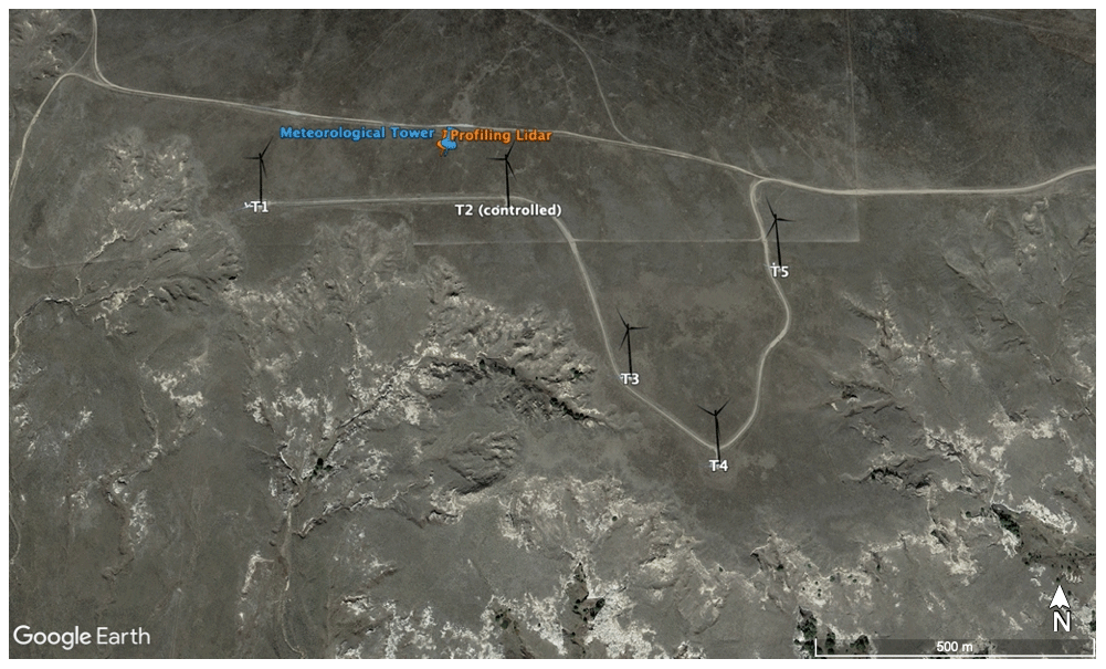
Figure 1Site of the wake-steering field campaign, focusing on flow from the north through five turbines (T1–T5), with wake steering applied to T2 to benefit T3; inflow measurements come from a co-located meteorological tower and profiling lidar upstream. Map data from Google, © 2023 CNES/Airbus, Maxar Technologies, USDA/FPAC/GEO.
2.2 Data sources
To characterize inflow conditions, high-frequency data from a meteorological mast were considered along with time-averaged data from a co-located profiling lidar. These sensors were located approximately 160 m upwind from the leading control turbine. The met mast provided high-frequency measurements of velocity (three components), virtual temperature, humidity, and pressure. All measured quantities used for model input and validation are summarized in Table 1.
Table 1Meteorological measurements used in this study for MMC input (I) and validation (V).
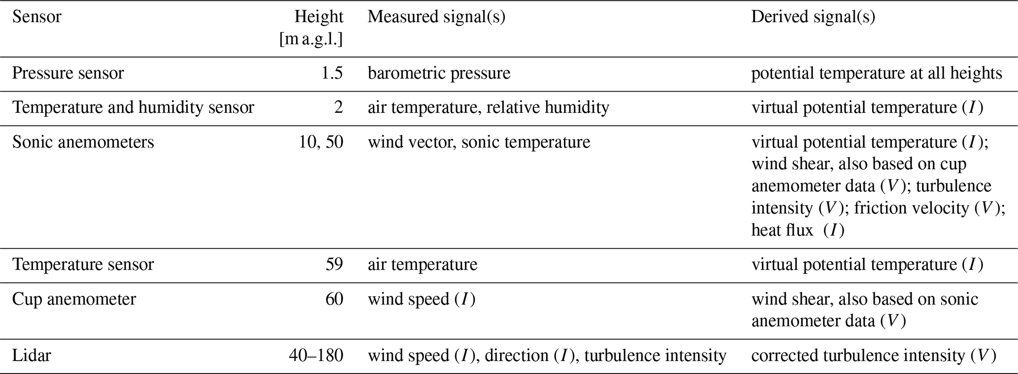
A number of quantities were derived from the met mast measurements. Potential temperature calculations were based on pressure profiles, assumed to decay exponentially according to a scale height H. H was estimated from the nearest sounding data, collected over 300 km away, to be 8 km. The pressure is thus evaluated as , where pobs is the pressure measured at 1.5 m above ground level (a.g.l.). Virtual potential temperatures were then calculated from the same estimated pressure profile, assuming the relative humidity (at 2 m a.g.l.) was constant with height over the met mast. Vertical momentum and heat fluxes describing surface conditions and atmospheric stability were calculated from sonic anemometers.
The lidar data had a range gate of 20 m and a maximum range of 260 m a.g.l.; the actual maximum range observed during the case study was 180 m. To address any possible bias in the measured turbulence due to cross-contamination effects, lidar measurements at 60 m a.g.l. were compared with cup anemometer measurements at the same height. A weighting function was developed based on this comparison and applied to lidar-measured turbulence intensities at 60 m and above. In general, the lidar overpredicted turbulence intensity (TI) by a factor of 1.10 (median; interquartile range 1.01–1.25).
In addition to the meteorological measurements, turbine operational data including power output and yaw offsets were available from NREL-installed instrumentation packages on turbines T2 and T3. Supervisory control and data acquisition (SCADA) signals were also available for all turbines. Quality assurance was performed on the SCADA data using the NREL instruments. Because of the tendency of yaw signals to drift over time, the NREL experimental team regularly estimated corrections to the SCADA signal to more accurately represent the instantaneous turbine yaw position.
2.3 Case study selection
A study period was identified based on the availability of quality-controlled lidar wind and load data (for the study of Shaler et al., 2023). The availability of lidar data was considered essential for this study because the lidar captures more inflow characteristics than point measurements of wind conditions. For quality control, the lidar wind data were filtered to remove data points with a carrier-to-noise ratio below −22.5 dB, while the load data were filtered by turbine status. Only periods during which the controlled turbine (T2) and downstream turbine (T3) were operating nominally (based on turbine status codes) and producing power were considered. From the quality-controlled data, candidate periods were selected with north–northwesterly winds between 320 and 350°, the predominant wind sector. This wind direction range includes the direction of alignment at 324°, at which the controlled turbine (T2) directly wakes the immediate downstream turbine (T3).
Given these filtering criteria, 17 baseline (without steering) and 21 controlled (with steering) 10 min periods were found between December 2019 and January 2020, the 2 months of the campaign in which turbines T2 and T3 were fully equipped with load instrumentation. The majority of the available data satisfying these criteria corresponded to atmospheric conditions with low hub-height wind speed and turbulence intensity: m s−1 and %, respectively. Out of these 38 candidates, 12 nearly consecutive 10 min periods – 5 baseline, 7 controlled – occurred on 26 December 2019 after midnight, starting from 07:48 UTC (local time (LT) is UTC−7 h) and ending at 10:58 UTC. These 12 periods are the focus of the present case study.
3.1 Terrain effects
Given northerly flow conditions, the wind flows toward the test site over mildly sloping terrain. For northwesterly flow (from 315°), the change in elevation is less than 40 m over approximately 4 km (Fig. 2); the variation in elevation is less for wind directions closer to northerly, i.e., winds from the north (360°). Downwind of the test site, the terrain changes abruptly as the wind flows down an escarpment. The effect of this terrain on local wind conditions is not known. A preliminary assessment of measurements from the met mast at 10 m, over a 24 h period (25 December 2019 at 12:00 UTC to 26 December 2019 at 12:00 UTC, encompassing the 12 study periods), revealed nonzero mean vertical velocities ∼𝒪(0.1) m s−1. These velocities are an order of magnitude larger than typical large-scale vertical motion, fluctuating with an approximately 4 h period. Significant variability in the mean hub-height wind direction was observed over the entire duration of the case study. Whereas the wind direction ranged from approximately −135° (southwesterly) to 90° (easterly), the near-surface winds as measured by a sonic anemometer varied across all directions, from −180 to 180°. No correlation was observed between the instantaneous vertical velocities and the elevation changes (upstream or downstream) or zonal (east–west) winds. In combination, these observations suggest the occurrence of more complex unsteady, three-dimensional flow. These wind direction shifts near the ground may suggest atmospheric wave phenomena and may be associated with turbulence intermittency (Sun et al., 2004).
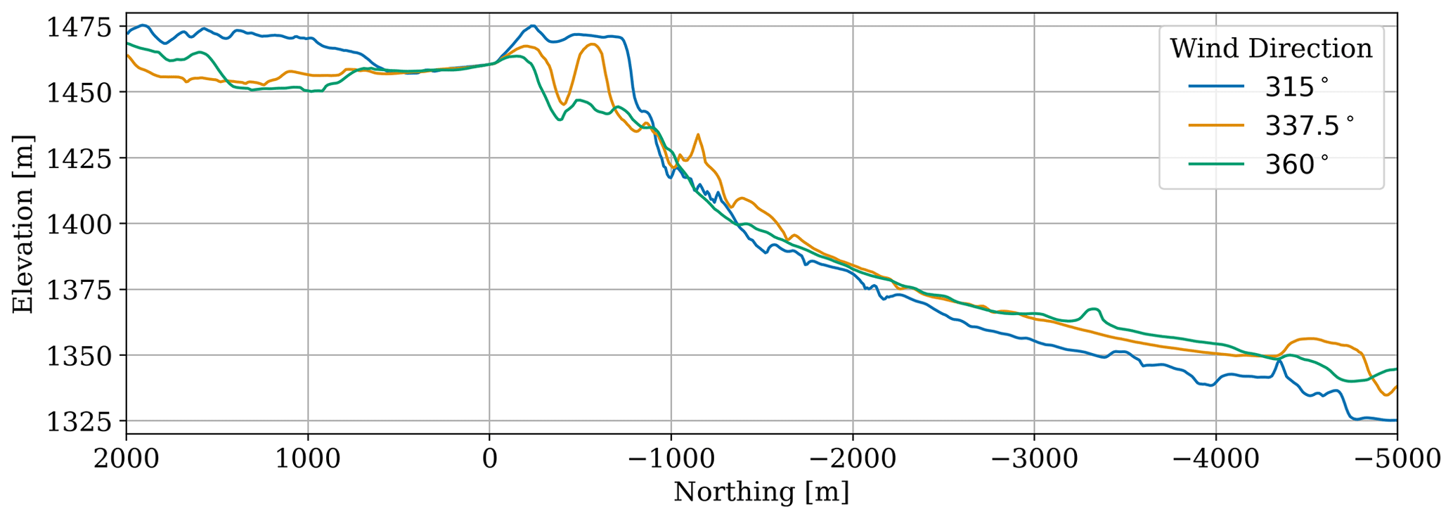
Figure 2Terrain transects for different northerly inflow directions, centered at the meteorological tower (Fig. 1).
Mesoscale conditions during the case study were initially simulated with the WRF NWP model (details in Appendix D). The innermost nested simulation domain had 3 km grid spacing. Results were insensitive to the choice of reanalysis dataset (the Global Forecast System; the European Centre for Medium-Range Weather Forecasts Reanalysis, version 5; and the Modern-Era Retrospective analysis for Research and Applications, version 2) and initialization time (8, 14, and 20 h before the period of interest). While it is possible that all these datasets did not adequately capture synoptic conditions during this period, a likely factor contributing to the inaccuracies in the mesoscale analysis is the effect of the local topography. Terrain data are available at 30 arcsec resolution (≈1 km), but the simulated 3 km grid spacing effectively smooths the land surface. Using a finer grid resolution, however, risks simulation within the terra incognita regime (Rai et al., 2019). Thus, at 3 km mesoscale spacing, an elevation difference of ∼100 m is modeled (Fig. 2) albeit without the correct local slope on the escarpment. Some variability between conditions at the test site and surrounding mesoscale grid points was seen in the WRF simulation ensembles, but none captured the time history of wind conditions at the met mast. This offers evidence that local terrain or downstream flow effects such as drainage may be important drivers of the microscale flow.
3.2 Precipitation
Analysis of synoptic weather charts indicated the presence of a stationary front that persisted throughout the period of interest. Depending on the moisture in the air and the atmospheric pressure, stationary fronts may be conducive to cloudiness and precipitation. This was confirmed by the National Oceanographic and Atmospheric Administration (NOAA) Next-Generation Radar (NEXRAD), a network of S-band weather radars. Long-range base reflectivity from scans at 0.5° elevation was downloaded from the NEXRAD data archive, hosted by the NOAA National Centers for Environmental Information. The reflectivities (>20 dBZ) indicated possible light rain in the region on 26 December 2019 from 23:30 to 02:30 UTC the following day (see shaded time periods in Fig. 3).
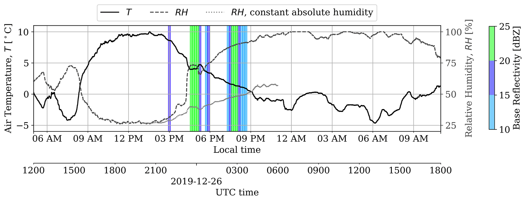
Figure 3Air temperature (T) and relative humidity (RH) measured on the meteorological mast at 2 m a.g.l.; the shaded regions indicate 5 min periods with 10–15 dBZ (light blue), 15–20 dBZ (dark blue), and 20–26.5 dBZ (green) base reflectivity.
Local met mast observations revealed complex transport processes, the characterization of which is beyond the scope of the present work. The onset of possible precipitation corresponded to a sharp increase in relative humidity (RH) at 23:00 UTC (Fig. 3). However, this is the same time as the evening transition when RH typically increases due to a decrease in temperature. To illustrate that this pronounced change is not due to diurnal temperature variation alone, RH is extrapolated forward in time assuming that the absolute humidity remains constant from 20:00 UTC, prior to the precipitation event. This hypothetical exercise shows that after the precipitation event, RH would have been significantly lower than observed. Therefore, the moisture content in the air is likely to have increased in reality. Observations also indicated the occurrence of temperature advection after midnight local time (Fig. 3). Since large-scale warm air advection from the north (given northerly flow) is unlikely, these observed changes in air temperature must be driven by mesoscale processes.
This work adapts existing MMC methods to the present case study based on observational data constraints. Unlike previous studies that successfully applied profile assimilation with observational data alone (Allaerts et al., 2023), initial and boundary conditions in this case are not fully specified over the entire microscale domain. This limitation, combined with the previously presented meteorological considerations (Sect. 3), necessitates a more tailored computational approach. Section 4.1 describes applicable coupling methods; the following subsections detail the curation of the mesoscale data, the reconstruction of that data to span the simulation domain over the entire simulation period, and a modified profile assimilation strategy that is compatible with the assumptions made during data reconstruction. The validity of applicable MMC methods is assessed in the “Results and discussion” section (Sect. 5). Methods presented here are code agnostic; for reference, the models used in this study (the Simulator fOr Wind Farm Applications (SOWFA) for LES and OpenFAST with the Reference OpenSource COntroller (ROSCO) for aeroservoelastic turbine simulation) are described in Appendix A.
4.1 Overview
Given the complex meteorological conditions described in Sect. 3, three simplifying assumptions have been made to make the computational problem approachable for wind energy modeling. The first assumption is that the downstream flow down the escarpment has a negligible effect on simulated hub-height winds and, consequently, a negligible effect on wind turbine performance, loads, and wakes. Related assumptions are that the observed mean vertical velocity and any inflow variation induced by upstream terrain also have a negligible effect on simulated hub-height winds. In combination, these assumptions permit modeling of the entire region as having flat terrain. The final assumption for this case study is that for wind energy quantities of interest, the transport of moisture (seen in Fig. 3) does not need to be explicitly modeled. Instead, the effect of moisture on the total air density is implicitly captured through virtual temperature quantities.
Incompressible LES is used to resolve the locally observed atmospheric conditions and provide mean flow and turbulence information at high spatiotemporal resolution. This LES flow field information will complement the field measurements and provide realistic turbulent inflow conditions for coupled aeroservoelastic turbine simulations. The evolution of local conditions is likely driven by larger-scale – i.e., mesoscale – nonstationarity. These time-varying conditions may be achieved by introducing source terms into the governing momentum and/or temperature equations that “nudge” the solution toward known reference values with Newtonian relaxation (Stauffer and Seaman, 1994). To this end, MMC strategies are applied to realistically evolve the LES according to observed conditions and are briefly reviewed here; a comprehensive overview can be found in Haupt et al. (2023).
Assumption of flat terrain permits a horizontally homogeneous ABL simulation setup, which lends itself to several different MMC approaches (Table 2). These approaches are equally applicable to scalar and vector atmospheric field quantities. The simplest approach is to apply a time-varying uniform forcing, which drives the simulated wind or temperature field to match the mesoscale data at a single height level. This single-level forcing may be applied if full profiles are not known or the focus is on specifying a quantity at a particular height (e.g., wind speed at hub height). To exercise more control over the background flow than the single-level approach, full wind and temperature profiles may be assimilated in the LES. Profile assimilation differs from observational or analysis nudging, e.g., in a mesoscale four-dimensional data assimilation framework (Liu et al., 2007; Telford et al., 2008) or microscale data assimilation in a detached eddy simulation (Zajaczkowski et al., 2011), in which a combination of temporal, vertical, and/or horizontal weighting functions is applied in three dimensions, typically near the surface. This work uses a time–height profile assimilation approach without any spatial or temporal weightings. Profile assimilation forces essential planar-averaged quantities (horizontal velocity components, virtual potential temperature) to match mesoscale flow information by adjusting the instantaneous magnitude of momentum and/or temperature sources (Allaerts et al., 2020). These source terms are horizontally uniform, taking advantage of horizontal homogeneity. This approach was originally developed and validated with WRF mesoscale forcing and more recently demonstrated with observational forcing (Allaerts et al., 2023). Using time–height flow field information based on local observations (described in Sect. 2.2) implicitly captures all relevant mesoscale effects, including local terrain and weather.
Table 2Summary of MMC strategies applied in the current study.
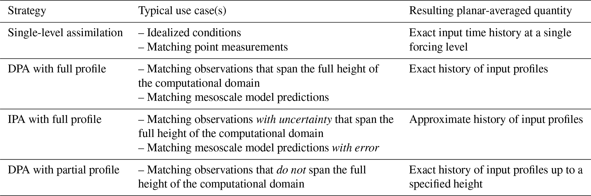
Mesoscale-to-microscale coupling enforced through profile assimilation in the LES is derived from the instantaneous error between the simulated microscale planar average and the local mesoscale flow. This forcing may be either directly applied (i.e., direct profile assimilation, DPA) or indirectly applied (i.e., indirect profile assimilation, IPA). These two approaches are described in detail and compared in Allaerts et al. (2020). In the indirect approach, the applied forcing is a polynomial representation of the direct forcing profile – this introduces interdependence between the forcing at each height level, constituting a “nonlocal” approach. Consequently, the polynomial approximation spatially filters the forcing profile and permits the microscale LES to instantaneously deviate from the enforced mesoscale trend. DPA and IPA may be thought of as strong and weak coupling strategies, respectively. All MMC approaches have been considered for the wind field, whereas only the single-level assimilation is applicable based on temperature point measurements. As a final note, the aforementioned approaches provide mechanisms for matching the time history either at a single level or at all levels – there is no intermediate approach for matching the time history at a subset of levels. This has motivated the partial profile assimilation approach detailed in Sect. 4.4.
4.2 Initial conditions
Considering the complexity of the observed atmospheric dynamics during and leading up to the period of interest (Sect. 3.2), the MMC LES was initiated during the previous morning, which saw more canonical conditions, allowing the flow to fully develop prior to the possible precipitation event in the afternoon. Because information about the upper atmosphere is not available from local measurements, sounding data were used to inform the initial profiles of wind and virtual potential temperature. Wind and temperature profiles spanning the entire height of the computational domain were derived from the closest upwind sounding site, located approximately 340 km to the north. Even though these are not strictly local conditions, the virtual potential temperature profiles in particular are useful for characterizing the height and strength of the capping inversion, which modulates the growth of the daytime convective boundary layer (CBL). With sounding data available every 12 h at 00:00 and 12:00 UTC, the closest starting time was 12:00 UTC (05:00 LT) on 25 December 2019, nearly 20 h prior to the load study periods. This early start time is expected to allow adequate time for the turbulence to develop in the microscale domain and adjust to any inconsistencies between the distant initial sounding and the local conditions.
Sounding measurements extended from the ground up to more than 30 km a.g.l., significantly higher than the top boundary of the simulation domain. To adapt the distant sounding to local conditions, the lowest 200 m of the wind and virtual potential temperature profiles was replaced with local site measurements (Fig. 4). These profiles were linearly interpolated between measurement heights. The soundings also provided an estimate of the temperature lapse rate above the capping inversion, in this case 4 K km−1. This same initial value was prescribed as the fixed temperature gradient on the upper boundary.
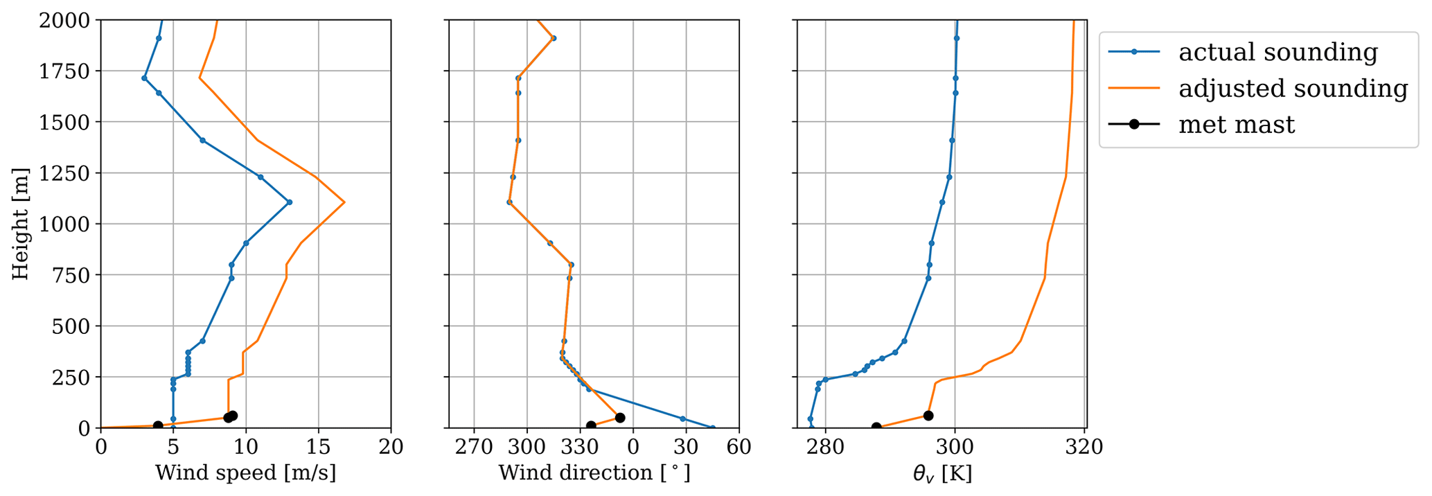
Figure 4Upwind sounding data, adjusted with local measurements to be used as initial conditions.
4.3 Surface boundary conditions
The surface wind and temperature boundary conditions (BCs) are based on Monin–Obukhov similarity theory (MOST). Aerodynamic roughness has been assumed to be uniform with a nominal value of 0.1 m. In general, there is significant uncertainty associated with modeling surface conditions, in particular when deciding how to specify the surface heat flux (see, e.g., Mirocha et al., 2015). Specifying the surface temperature and deriving the heat flux from MOST may be more physically consistent, especially for moderately to strongly stable conditions, by allowing for dynamic variation in the heat flux according to the local resolved temperature field (Basu et al., 2008a; Kumar et al., 2010). A preliminary study (not shown) compared BCs that specified kinematic heat flux (derived from 10 m sonic anemometer measurements) with those that specified surface temperature (measured by a 2 m probe). Both time-varying BCs used input time histories averaged to 10 min intervals. During the daytime, the heat flux BC provided better agreement with the measured turbulence intensity at 50 m a.g.l., whereas during the nighttime, both BCs performed similarly. A heat flux BC was therefore used to enforce surface temperature conditions with the stipulation.
There exists a caveat with regard to the surface BC for wind and the DPA approach. Direct profile assimilation forces the planar average to match an input wind profile so that the lowest computational cell (adjacent to the surface) that is set by the BC will always have its value adjusted to match the input wind profile at that height. Therefore, the input profile always supersedes the value imposed by the BC, and the assumed roughness length only has an effect on the simulated wind fields when using single-level forcing or IPA.
Daytime convective conditions were simulated by specifying the kinematic heat flux calculated from sonic anemometer data at 10 m a.g.l. The preliminary study found that an assumption of a constant-flux surface layer was invalid – specifying the 10 m heat flux at the surface resulted in only 80 % of the observed flux at 10 m, which had a maximum of 0.1 K m s−1 (indicative of weakly convective conditions). Therefore, the specified surface heat flux was increased by 25 % to match observed conditions. In the nighttime, the empirical rescaling was not applied. To more accurately represent the observed nocturnal temperature advection (Fig. 3, after midnight LT), the observed temperature on the met mast at 59 m was also assimilated.
4.4 Partial profile assimilation
A wind time–height history was reconstructed for MMC (Fig. 5) following a procedure specific to the data available for this study. The procedure included quality control, fitting instantaneous profiles to a canonical power law, and interpolation and is fully detailed in Appendix C. The final reconstructed wind speed profiles had wind shear with a power-law exponent (α) of approximately 0.1 in the daytime between 09:00 and 14:30 LT; then, the shear increased, varying between α=0.2 and 0.4 throughout the remainder of the afternoon and into the evening. Between 22:00 LT and midnight, the shear was highly variable and not well defined by the power law when taking into account all available wind measurements. From 01:00 LT and onward to the next day (during the turbine study period), α similarly varied between 0.2 and 0.5.
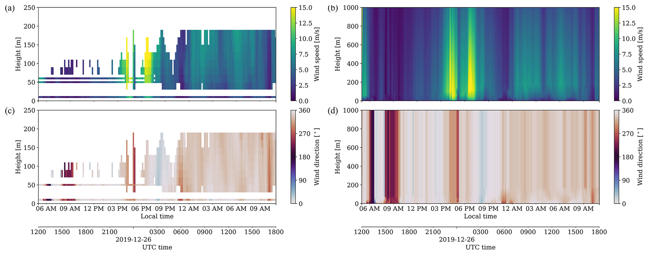
Figure 5Available wind speed and direction measurements, including sonic anemometers, a cup anemometer, and lidar, shown up to the farthest lidar range gate (a, c); reconstructed time–height wind profiles, spanning the vertical extent of the computational domain (b, d).
The flow field reconstruction provides a representation of how the background wind profiles evolved, but the available measurements did not support any reasonable approximation of how the temperature profile evolved. Information about the thermal stratification and ABL height would have informed the reconstruction of the wind profiles above the ABL; moreover, temperature profile assimilation could have been performed alongside the wind profile assimilation. Instead, the evolution of the temperature profiles in the current study is more idealized, dictated only by initial and surface conditions.
An additional consideration is needed because the height of the ABL is not known. The reconstructed winds (Fig. 5) are only valid within the ABL, and at the top of the ABL the boundary layer winds should transition to geostrophic and thermal winds. However, it is not known whether a geostrophic or thermal wind balance exists or how the free atmosphere interacts with the ABL. An additional assumption must be made, falling back on a simpler assimilation strategy. Instead of having the large-scale forcing vary in both time and height, the forcing in the free atmosphere is assumed to be uniform with height and vary in time only. Then, to both capture local mesoscale variability near the ground and allow realistic ABL evolution aloft, the wind forcing profile is blended from the forcing profile derived from profile assimilation to a constant value. Ideally, transition between the height-varying ABL forcing and the uniform free-atmospheric forcing would occur at the instantaneous ABL height, but because this height is not known a priori, the transition between the forcing regions occurs above 180 m, the highest available measurement. Above 180 m, the vertical gradient of the forcing profile is linearly scaled to zero. The thickness of the transition layer was chosen to be 100 m. This approach has recently been applied in a similar fashion with virtual potential temperature profiles (Jayaraman et al., 2022, “hybrid II” strategy).
The LES setup is detailed in Appendix B. Section 5.1 first presents the measurement-driven precursor simulation of the diurnal cycle leading up to and during the case study period. Then, Sect. 5.2 presents LES results with turbines represented as actuator disks, driven by the large-scale nonstationary conditions of the precursor. Section 5.3 derives additional insights from these results.
5.1 Diurnal cycle simulation with MMC
Applicable MMC approaches are considered for the selected case day. These include the simple single-level approach applied at 50 m a.g.l., the height of the highest sonic anemometer; the DPA and IPA approaches of Allaerts et al. (2020); and the partial profile assimilation approach detailed in Sect. 4.4. Separate assimilation approaches were considered for daytime and nighttime, with the switchover occurring at 14:00 LT, just before the measured change in atmospheric conditions (Fig. 3) and an increase in lidar data availability (Fig. 5). The temperature advection during both the diurnal and the nocturnal periods (Fig. 3) was not captured from the surface conditions alone (results not shown); therefore uniform forcing based on the temperature probe at 59 m height was applied. To highlight the impact of the single-level temperature assimilation, the simplest single-level wind forcing (at 50 m a.g.l.) case is considered with and without temperature forcing during the daytime. Even when temperature and humidity do not change significantly due to weather, assimilating local temperature observations can change the structure of the capping inversion, which in turn alters the geostrophic wind and, consequently, also affects the veer throughout the ABL (Fig. 6). All other simulations therefore included single-level temperature assimilation.
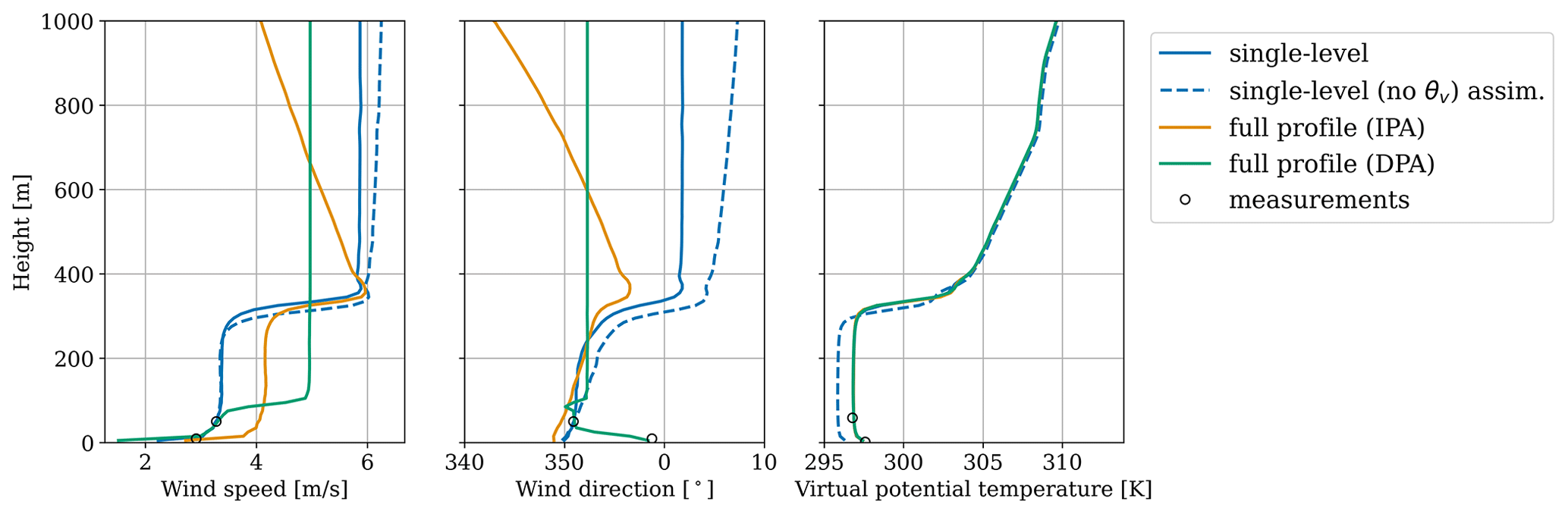
Figure 6Example daytime CBL profiles at 13:00 local time (LT) for various mesoscale forcing approaches; the markers indicate the available sonic anemometer measurements.
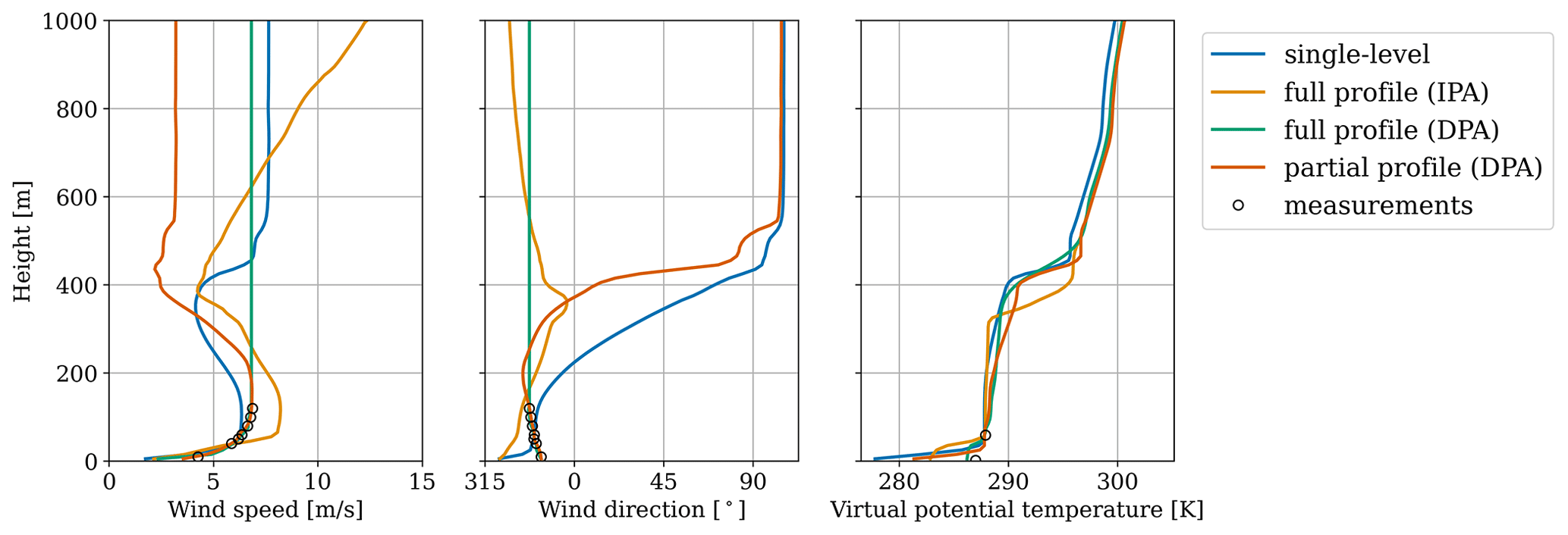
Figure 7Example nighttime stable boundary layer profiles at 01:00 LT for various mesoscale forcing approaches; the markers indicate the available sonic anemometer and quality-controlled lidar measurements.
The paucity of daytime measurements adds uncertainty to the flow field reconstruction (Fig. 5) and results in varied wind profiles (Fig. 6). DPA appears to predict an extremely shallow convective ABL, while IPA appears to predict a sharp low-level jet in the daytime – neither of which appears plausible. The possibility of unbounded IPA behavior is a known issue (Allaerts et al., 2023). In contrast, the single-level results (assimilating winds at 50 m) predict the most reasonable representation of the weakly convective boundary layer and overlying free atmosphere while also capturing the observed wind speed at 10 m. Because the conventional MMC methods produced satisfactory results, the partial profile approach was not applied in the daytime.
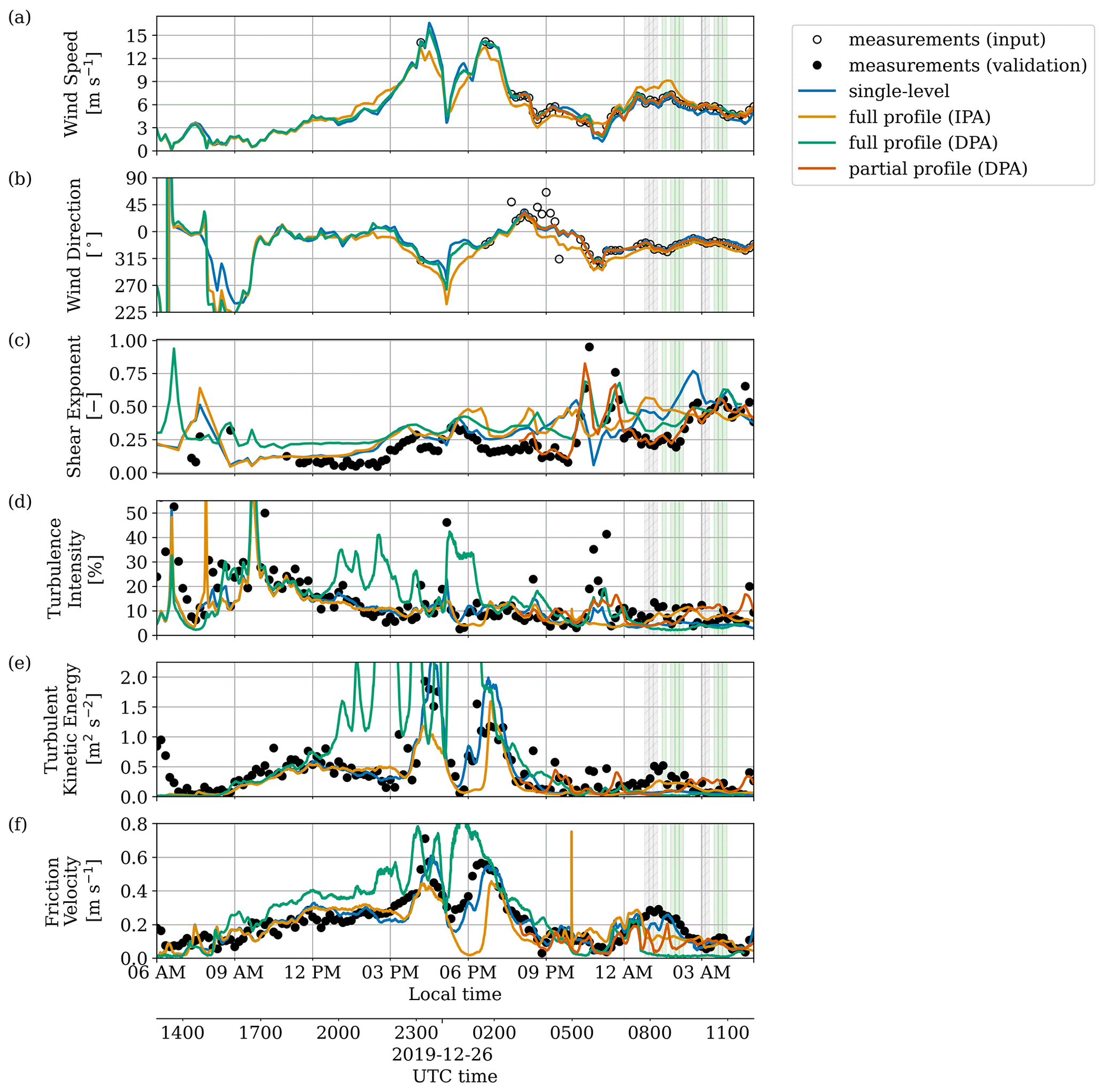
Figure 8Simulated atmospheric conditions from the coupled LESs (lines) in comparison with measurements (symbols): hub-height lidar wind speed (a) and direction (b), power-law shear exponent estimated from met mast anemometers (c), 50 m sonic anemometer turbulence intensity (d), 50 m sonic anemometer turbulent kinetic energy (e), and 10 m sonic anemometer friction velocity (f); the 10 min periods of interest for turbine analysis are highlighted (gray shading with hatch marks represents no commanded yaw offset, and green shading represents a commanded offset).
In the nighttime, a larger range of wind speed and direction values are observed than in the daytime; the thermal structure of the boundary layer also shows more variation due to the cumulative differences in both wind and temperature profiles over the course of the day (Fig. 7). Single-level assimilation is unable to represent the observed wind profile, instead predicting a very shallow low-level jet. The IPA results are once more suspect, with high wind speed and shear simulated at the top of the computational domain. Therefore, plausible results include the full- and partial-DPA simulations, with pronounced differences in the free atmosphere. Under these conditions, the partial-DPA LES predicts lower wind speeds aloft that describe a nocturnal low-level jet.
Quantities of interest were calculated for the four approaches considered (Fig. 8). A distinction has been made in the reference measurements between what was included in the assimilation data (input) and what was used for validation. Note that all of the LES results presented therein used single-level temperature assimilation based on the 59 m met mast measurement, and the caption describes the treatment of time-varying wind conditions. The time history of the simulated case day clearly demonstrates that the mean wind speed and direction trends from the experiment are generally reproduced. Because the IPA approach allows the microscale to deviate from the input mesoscale data – a potentially desirable mechanism for modulating mechanical turbulence production (Allaerts et al., 2020) – some differences ∼𝒪(1) m s−1 are seen. The shear exponent was estimated from 10 min wind speeds, measured by met mast anemometers at 10, 50, and 60 m a.g.l., by fitting to the power law (Fig. 8c, values with coefficient of determination R2>0.9 shown). Wind shear is slightly overpredicted during the daytime and evening transition, even with DPA. This is because the shear in the reconstructed profiles is also influenced by the available lidar wind measurements (Fig. 5). In the nighttime stable boundary layer, there is significant variability between MMC approaches, but partial profile assimilation is able to represent the observed time history of the shear exponent throughout the entire simulation – including two high-shear events at 22:40 and 23:40 LT. Turbulence intensity, TKE, and friction velocity (Fig. 8d–f) are not directly specified but also capture the observed trend in all cases. Excluding outliers, the TI in the daytime is several times higher than in the nighttime: 20 %–30 % compared to 5 %–10 %. TKE provides a similar assessment that also takes into account vertical velocity variance and does not have sensitivity to low wind speeds. For most of the case day, the DPA results track the observed friction velocity (u*), confirming the relationship between shear stress (described by u*) and the wind shear in the profile that is exactly matched by DPA. Deviations from observations are seen in the single-level and IPA results, which do not exactly match the observed wind shear and may be sensitive to the choice of roughness height (see discussion in Sect. 4.3). At night, the turbulence is intermittent. Some of this variability is captured with the various assimilation approaches, but the timing and magnitude do not exactly match observations (from 22:00 LT to the end of the simulation) in terms of TI and friction velocity. In the early morning after 01:00 LT, the friction velocity at 10 m is only captured by the single-level assimilation. Considering that this occurs during stable conditions, this discrepancy may be a consequence of inadequate grid resolution near the surface (10 m; see Appendix B for additional LES details).
5.2 Turbine simulation during study period
Results from the SOWFA–OpenFAST aeroelastic turbine simulation and the engineering-fidelity FLOw Redirection and Induction in Steady State (FLORIS) wake model are compared with the power signal recorded by the wind farm SCADA system. The ABL LES for the turbine study was restarted from the daytime CBL simulation with single-level wind and temperature forcing. From this fully developed turbulence field, the evening transition and nocturnal stable boundary layer were simulated with partial wind-profile DPA and single-level temperature assimilation. Mean wind conditions from LESs showed reasonable agreement with lidar observations (Fig. 9). During the selected turbine-analysis periods (with and without wake steering), the simulated wind speed ranged between 4.7 and 7.1 m s−1, the wind direction was approximately north–northwesterly, and the TI ranged between 0.02 and 0.08. The mean absolute errors (MAEs) for these three quantities were 0.19 m s−1, 1.5∘, and 0.031, respectively. While the TI is in a similar range as the observations, the timing of the turbulence intermittency is not reproduced. These LES wind conditions were also used as inputs to FLORIS.
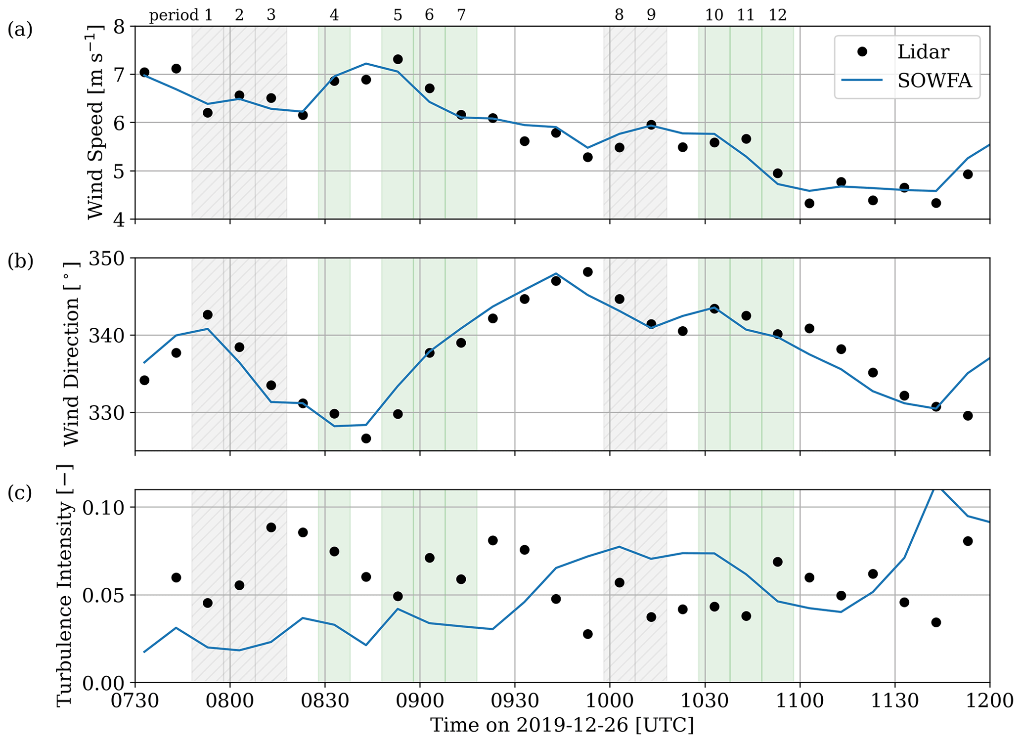
Figure 9The 10 min mean wind speed, mean wind direction, and turbulence intensity at hub height throughout the turbine study during periods without any commanded yaw offset (gray shading with hatch marks) and a commanded wake-steering offset (green shading). Quantities are plotted at the center of each 10 min averaging interval.
Wake steering is toggled on and off by manipulating the input yaw signal to the turbine controller, resulting in an intentional yaw misalignment. Periods without any commanded yaw offset will also see unintentional yaw misalignment due to turbulent fluctuations of the wind vector magnitude and direction. Similarly, the actual yaw offset achieved will differ from the commanded optimal offset due to turbulent fluctuations (Fig. 10c). Note that SCADA data are available throughout the study period, but only the 10 min periods during which all NREL-collected data channels passed quality assurance and quality control checks have been highlighted.
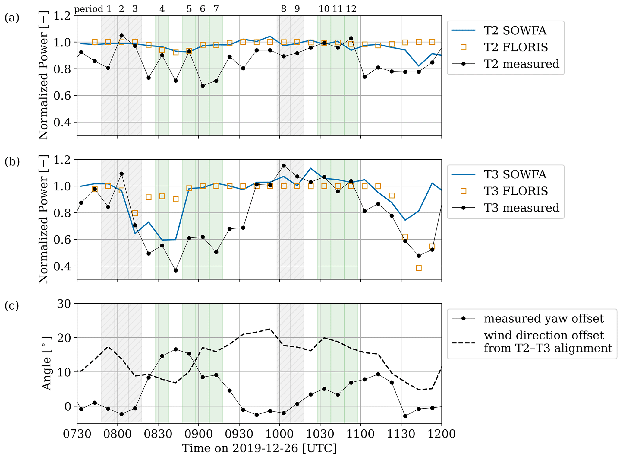
Figure 10Normalized 10 min mean power for turbines T2 and T3 (panels a and b, respectively) during periods without any commanded yaw offset (gray shading with hatch marks) and a commanded wake-steering offset (green shading). The actual measured offset is given in panel (c), along with the degree to which T3 is directly waked by T2. Quantities are plotted at the center of each 10 min averaging interval.
All reported power output (Fig. 10) has been normalized by the mean power produced by freestream reference turbines T1 and T5. Between 07:48 and 08:18 UTC (periods 1–3), the true measured yaw offset is approximately 0∘. However, the wind direction is offset from the T2–T3 alignment direction (324°) by 9 to 17°, resulting in partial waking of T3 by T2 (period 3 is shown in Fig. 11a). During these periods, the simulated and measured wind speed and direction differ by 0.2 m s−1 and 2°, respectively, but the TI is underpredicted in the LES by 0.07. Both FLORIS and SOWFA predictions are comparable to the measured power from T3 at this time (Fig. 10), with errors of +0.09 and −0.06, respectively.
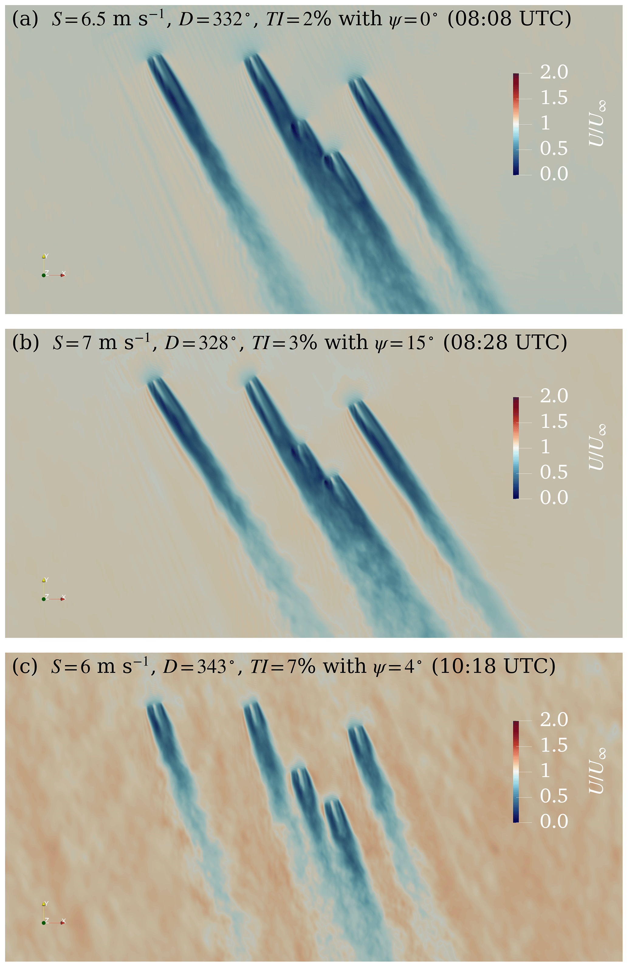
Figure 11The 10 min mean horizontal wind speed fields at wind turbine hub height predicted by LES on 26 December 2019, normalized by the inflow wind speed. The mean wind speed (S), wind direction (D), turbulence intensity (TI), and actual yaw offset (ψ) are given for periods with (a) partial waking, without wake steering; (b) partial waking, with wake steering; and (c) nearly waked conditions, without wake steering.
The subsequent wake-steering period from 08:28 UTC (period 4) had a simulated wind speed and direction in agreement with measurements to within 0.1 m s−1 and 2°, but the TI was still smaller by a factor of 2. At this time, the largest yaw offset of all studied periods, 15°, was observed. This was slightly less than the commanded offset of 17°. Turbines T2 and T3 were also the most closely aligned out of all studied periods, with an alignment direction offset of 8°. Overall, this resulted in a similar partial-waking scenario to period 3 without steering (Fig. 11b). During this period, SOWFA correctly predicts the waked conditions, whereas FLORIS appears to represent unwaked conditions, with normalized power errors of +0.37 and +0.04 for FLORIS and SOWFA, respectively. In the remainder of this steered period from 08:48 to 09:28 UTC (periods 5–7), both SOWFA and FLORIS predict completely unwaked conditions. After 09:08 UTC, the wind direction appears to be sufficiently offset from the T2–T3 alignment direction such that, despite a reduction in wake-steering offset, the downstream turbine produces power as if it was in the freestream.
During the next highlighted periods without steering from 09:58 UTC (periods 8–9 in Fig. 10), there appears to be further interplay between the wind direction and turbine yaw. During this time, the simulated wind speed, wind direction, and TI agree with measurements to within 0.3 m s−1, 2°, and 0.03, respectively. Even though the actual yaw is near zero, there is enough wind direction offset such that the T3 power output is comparable to the freestream turbines until 10:48 UTC (period 9 is plotted in Fig. 11c). Around this time, there are several 10 min periods observed in the field (three periods) and in the LES (four periods) during which the downstream turbine power production exceeds freestream power by ≥5 %. The maximum excess power production is 1.15 and 1.13 for the actual turbine and LES, respectively, and occur at different times. During the nearly waked conditions between 10:18 and 10:28 UTC when there was 13 % more power predicted than in the freestream turbines, the excess power produced by T3 is associated with a 2 %–4 % increase in wind speed experienced by the turbine as sampled by the LES. Even though this estimated wind speed increase is based on a spatial average over the rotor disk with some sensitivity to the upstream location, it agrees with the law (P and U∞ are power output and freestream wind speed, respectively).
In the following wake-steering periods (periods 10–12), the simulated wind speed, wind direction, and TI agree with measurements to within 0.4 m s−1, 2°, and 0.03, respectively. The operating conditions are similar to the previous periods – the achieved yaw offset angles were relatively low (5–7°), while the alignment direction offset was relatively high (17–20°). Overperformance is consistently observed in the LES and exactly matches the actual T3 power output for two out of three periods. During period 11, however, the actual normalized turbine power momentarily decreases below 1 (0.96).
From approximately 11:38 UTC onward (Fig. 9), there appears to be a change in simulated mesoscale conditions seen in the wind direction and TI. The condition change appears to arise 10 to 20 min early, for wind direction and TI, respectively, compared to observations. This corresponds to the mismatch between the measurement and LES for both T2 and T3 (Fig. 10).
5.3 Discussion
Nocturnal stable boundary layers (SBLs), even without turbulence intermittency, are challenging to simulate (Bosveld et al., 2014a). Recalling that the lidar TI measurement has significant uncertainties and was corrected with another instrument only at a single height (below hub height), the TI MAE of 0.031 appears less egregious. Despite the mismatch in TI histories (Fig. 9), Fig. 10 shows good agreement between the LES and measured performance of T2 and T3 under partially waked conditions (periods 3 and 4; see Fig. 11a and b). Under nearly waked conditions (between approximately 10:00 and 11:00 UTC; see Fig. 11c), when T2's wake is close to impinging on T3, both LESs and measurements show some excess power production compared to the freestream turbines. The magnitude of this overproduction is similar, 13 % from LES and 15 % for the actual turbine, but occur at different times. Overall, in assessing the quality of the simulated inflow for predicting turbine performance, the quality of these comparisons suggests that the turbulence regime (TI<10 %) rather than the instantaneous magnitude of TI is the more important driver of turbine–turbine wake interactions. However, it is important to note that this difference in background turbulence may have a more pronounced impact on turbine loads than performance.
The most representative conditions for wake steering are periods 3 and 4, during which turbines T2 and T3 were the most closely aligned and achieved yaw offsets of 0 and 15°. Power predicted by LES during these periods was within 6 % of measurements. Simulated and measured power can have discrepancies when the T2–T3 alignment direction offset, combined with the instantaneous yaw offset, results in borderline waked conditions (i.e., partially or nearly waked). These borderline conditions may arise from small differences in the simulated and actual wind direction, e.g., between 08:48 and 09:28 UTC. Uncertainties in the wind field reconstruction may have further affected the quality of both the LES and the engineering model predictions.
In addition to the sensitivity to instantaneous wind direction, the actuator disks in the LES generate some numerical artifacts (the “streamers” seen emanating from the edges of the rotors in Fig. 11b). These types of artifacts, which may be obscured by the background flow under conditions with higher turbulence intensity, are due to application of a second-order central-difference numerical scheme with insufficient grid resolution to capture the velocity gradients around the rotor. This issue may be mitigated by filtering the actuator disk force distribution (Shapiro et al., 2022). To eliminate these numerical oscillations, the grid resolution would need to be increased by a factor of 106 to strictly satisfy a grid resolution constraint for grid Péclet number Pe≤2 (Xu and Yang, 2021), making a 4.5 h turbine LES far from tractable. However, spurious waves do not necessarily impact rotor performance and loads if 𝒪(10) grid points are simulated across the rotor (Revaz and Porté-Agel, 2021), a condition which is satisfied by the present LES setup.
The engineering and LES models are generally in agreement, with FLORIS clearly indicating when waking is expected to occur or not (Fig. 10). Differences were seen under three conditions: when FLORIS overpredicts the effect of steering (most pronounced around 08:28 UTC), when there is a wake-induced speedup (most notably at 10:18 UTC), and when there are dynamic inflow conditions (after 11:38 UTC). When steering is overpredicted, there is less waking and higher downstream turbine performance than observed in the LES and field measurements. This may be remedied in FLORIS by using the inflow TI as a tuning parameter (Doekemeijer et al., 2022). Because FLORIS does not simulate the flow field, effects such as blockage and the resulting speedup cannot be modeled unless a representative heterogeneous inflow field is provided as input (e.g., Branlard and Meyer Forsting, 2020). Similarly, FLORIS does not model wake motion, which would require a dynamic wake model. This actually translated into a more accurate prediction of T3 power production during the case study at around 11:38 UTC – because the simulated wind direction shift was earlier than observed (Fig. 9), the specified T2 position history (for 0° offset during this period) in the LES would have lagged behind the simulated wind direction change. This temporal shift in the LES resulted in an earlier reduction in waking on T3 and a large discrepancy between the LES and measurement. Under steady conditions, however, the engineering model continued to track the performance of T3 measured in the field.
The simulated wind field statistics (Fig. 9) are not in exact agreement with lidar observations, most notably in terms of the time history of the hub-height TI, which may be due to horizontal heterogeneity and terrain that have been neglected. The effects of heterogeneity can also be clearly seen in the variability in power produced by the upstream turbine T2 (Fig. 10). No relationship was found between the measured power from T2 and measured wind quantities in Fig. 9. Nevertheless, the resulting ABL simulation for the full day appears to be a reasonable representation of evolving mesoscale conditions – especially given the predicted turbine performance trends over a 4.5 h period (Fig. 10). As seen in Figs. 6 and 7, different plausible (and implausible) realizations of the ABL are possible. Differences in flow field realizations may be attributed to a combination of surface condition modeling, terrain, neglected large-scale vertical motions, and initial conditions. These uncertainties have varying degrees of importance depending on the time of day. During the daytime, any local terrain-induced wind variability is likely to be eliminated by turbulent mixing in the CBL, whereas in the nighttime this variability might be more pronounced. The ABL realization produced by partial profile DPA, ultimately used for the turbine study, results in a low-level jet with its nose near the top of the rotor (Fig. 7). Moreover, the formation and evolution of this jet may be responsible for the shear instability (Fig. 8c) and intermittent turbulence (Fig. 8d) that were observed. Considering the accuracy of the mean wind profiles that are predicted by the partial profile assimilation approach in the nighttime SBL (in terms of wind speed and shear exponent), the ad hoc transition thickness (100 m) describing the partial profile does not appear to have produced any appreciable wind profile anomaly.
The current partial profile assimilation approach is not intended to be a one-size-fits-all strategy. More sophisticated strategies are possible, for example, estimating the instantaneous ABL height from resolved turbulence fluxes to determine the extent of the partial profile. At the same time, the simple single-level method should not be ruled out either. Different MMC approaches may be used simultaneously, with one assimilation approach near the surface and another aloft. Furthermore, observational data can generally be supplemented with reanalysis or mesoscale model data. Instead of blending from an observation-derived forcing near the surface to a constant value aloft (as in Sect. 4.4), it is possible to use the mesoscale-modeled profile in the free atmosphere. This may be more accurate than incorporating sounding data at a single instant from over 300 km away. The surface conditions may also be specified by surface temperature instead of heat flux, which in this case would have avoided the ad hoc correction to account for the surface layer fluxes not being constant. Overall, the extent to which field conditions are reproducible with MMC depends on the nature of the background physical phenomena and their observability.
This work has provided insights into the practical applicability of MMC techniques given limited atmospheric data at a specific site. In this case, the limitations include the lack of information about the wind profile above 180 m in the nighttime and above 50 m in the daytime; the lack of information about the temperature profile apart from point measurements at 2 m and 59 m a.g.l.; and the inability of a numerical weather prediction model such as WRF to predict local mesoscale conditions. Atmospheric modeling challenges at this site include nonflat terrain, light precipitation, and unexpected temperature advection. As such, this case study is a major departure from canonical atmospheric and turbine operating conditions and is expected to build confidence in simulating a wider range of atmospheric conditions with large-scale nonstationarity.
The modeling challenges have been sidestepped by making appropriate assumptions. Assimilating local horizontal wind measurements captured possible terrain-induced flow variability. Even without temperature profile information, assimilating the virtual potential temperature history from a point measurement provided a zero-order representation of temperature and moisture advection. The simulated evolution of wind engineering quantities (wind speed, wind direction, and turbulence intensity) provided useful inputs to both an engineering wake model and a high-fidelity, LES-based aeroelastic model. Under waked conditions, the performance of the downstream turbine was satisfactorily reproduced by both models when given the actual measured yaw offset signal to steer the wake. In addition, the LES was also able to provide high-resolution information about wake dynamics, such as wake-induced speedups and wake-steering performance at low wind speeds. Even with high-fidelity inflow driven by local measurements, uncertainty still exists due to the dynamic variability in the inflow. This makes it challenging to disentangle the effects of wake steering from dynamic inflow effects during borderline conditions when a downstream turbine is very nearly or slightly waked. Overall, this simulation study offers insight into the short-term (intra-hour) variability of wake-steering performance. Even though wake-steering control strategies are designed with a focus on optimizing performance over the lifetime of a project and short timescales are not of primary concern, these results suggest that further wake-steering gains are possible and can inform a dynamic set point selection strategy. A direct outcome of this work is to enable validation of wake-steering loads, using even higher-fidelity aeroservoelastic simulations of turbines operating in the observed conditions. This is detailed in the companion paper by Shaler et al. (2023), which compares the simulated response of turbines T2 and T3 with SCADA signals and available load measurements.
The tailored MMC approach applied herein distills the relevant flow features from available data and highlights the challenges associated with microscale data assimilation. Flow field reconstruction challenges will always be site- and case-specific considering, e.g., the difficulty and cost of obtaining temperature profiles at high spatiotemporal resolution. To minimize assumptions needed to create a full wind and temperature profile history for LES, adequate resolution would ideally mean measurements with spacing comparable to the simulated grid spacing (e.g., less than 100 m), up to the top of the simulated domain (e.g., 1–2 km), at a sub-hourly sampling frequency. These guidelines should be taken into account when designing field campaigns to complement high-fidelity flow simulations. Even if high-resolution data were available, the microscale LES solution would still be sensitive to the chosen assimilation approach and whether it is desirable to exactly enforce measurements, i.e., the DPA approach. Engineering approximations such as IPA or partial DPA are attractive given that every dataset has unique limitations and uncertainties. Currently, no established approach is perfect – DPA can produce excessive turbulence, confirming previous findings (Allaerts et al., 2020); IPA forcings may be unrealistic. In this case, partial DPA provides a viable alternative when the mesoscale flow information is incomplete, especially when considering the dynamics of the nocturnal SBL in terms of evolving wind shear. In addition, this study demonstrates that profile assimilation is not necessarily needed to model an evolving CBL. Therefore, MMC forcing strategies present an opportunity for further generalization. Future work should focus on development of more robust, mathematically rigorous, and/or physically consistent forcing strategies.
A1 High-fidelity flow model: SOWFA
The Simulator fOr Wind Farm Applications (SOWFA; Churchfield et al., 2012), based on OpenFOAM version 6, was used to perform LESs of the field campaign site. SOWFA solves the momentum and potential temperature transport equations for a dry, incompressible flow with buoyancy effects represented by the Boussinesq approximation. The effects of moisture are accounted for through the use of virtual potential temperature in the temperature transport equation. Individual turbines are represented by actuator disk models (ADMs); these turbine aerodynamics models are loosely coupled to OpenFAST (Appendix A2) for a two-way, loosely coupled aeroservoelastic analysis. The term loose coupling is used here to describe a model with two separate dynamics solvers that exchange flow field velocities (from SOWFA to OpenFAST) and blade aerodynamic forces (from OpenFAST to SOWFA) at periodic intervals.
A2 Aeroservoelastic model: OpenFAST and ROSCO
OpenFAST (NREL, 2020) is a turbine model that solves the aeroservoelastic dynamics of individual turbines. Blade aerodynamics are calculated according to blade element theory from inflow provided by SOWFA. Momentum theory wake modeling is not needed because induction is captured by the SOWFA LES. Blade structural dynamics are calculated according to Euler–Bernoulli beam theory. The turbine controller is provided by the Reference OpenSource COntroller (ROSCO; Abbas et al., 2022), which has been tuned for this particular turbine model. In lieu of a yaw controller, the NREL-measured nacelle yaw angles of T2 (the controlled turbine) and T3 are specified for the simulated T2 and T3. The yaw positions of turbines T1, T4, and T5 are based on adjusted SCADA signals.
In creating the aeroservoelastic model for this study, NREL's reference model behavior, based on measurements of a similar DOE turbine (Santos et al., 2015), was found to differ from the turbines in the field campaign. Moreover, the exact turbine calibrations by the owner–operator are not known, which motivated the tuning of a site-specific turbine aeroservoelastic model. The dynamic response of T2 differed significantly from the other turbines in the test array. This work therefore employed two different ROSCO controllers, with different settings for T2 compared to the other turbines.
A3 Engineering wake model: FLORIS
The FLOw Redirection and Induction in Steady State (FLORIS) wake model is the same tool that was used to derive the yaw schedule for the field campaign. The version of FLORIS applied here includes more recent improvements, such as secondary wake steering and yaw-added wake recovery (King et al., 2021). Because it is not a time series analysis, FLORIS is only expected to accurately predict trends over the lifetime of a wind project (∼𝒪(10) years), aggregating the effects of interannual, seasonal, and diurnal variability while neglecting transient weather events. Agreement with instantaneous or 10 min averaged conditions is not necessarily expected.
All large-eddy simulations were run in a 4 km × 4 km × 1 km domain encompassing the wind farm. A precursor simulation evolves the diurnal ABL before, during, and after the turbine periods of interest; a subsequent turbine simulation restarting from the precursor introduces modeled turbines with mesh refinement around the individual turbines. The ABL turbulence field is resolved on a grid with uniform 10 m spacing and 0.5 s time steps. Subgrid-scale turbulence is modeled by a one-equation turbulent kinetic energy model (Deardorff, 1980). The effects of buoyancy are included through the Boussinesq approximation. Initial conditions (see Sect. 4.2) are specified by the nearest upwind sounding. On the lower boundary (Sect. 4.3), the surface shear stress is modeled following Schumann (1975), with an assumed aerodynamic roughness length of 0.1 m.
The precursor domain has periodic lateral boundaries: a no-slip lower boundary with specified time-varying, uniform surface heat flux and a free-slip upper boundary with a fixed temperature gradient (4 K km−1) dictated by the initial upper-air sounding. Nonstationary conditions are imposed through momentum and temperature source terms derived from a combination of met mast and lidar data as described in Sect. 4.1 and Appendix C. Mesoscale forcing profiles are updated at the standard wind engineering timescale, 10 min, which is shorter than the timescale of mesoscale flow evolution.
The turbine simulations restarted from the diurnal precursor simulation at 07:30 UTC on 26 December 2019, 18 min prior to the first load period of interest. Turbines are represented in the LES by the actuator disk model, which has been validated for both wake velocity deficit and power predictions in wind tunnel experiments (e.g., Neunaber et al., 2021) and simulations (e.g., Simisiroglou et al., 2017; Lignarolo et al., 2016; Revaz and Porté-Agel, 2021). The actuator disk is implemented within an actuator line modeling framework with 36 uniformly spaced actuator points in the radial direction. Disk forces are distributed in the azimuthal direction using a cosine-squared function such that the blade body force ranges from 1 at the current blade to 0 at the following blade. Blade body forces are uniformly distributed in the radial and axial directions with Gaussian functions with a width of 3.5 m. A Glauert correction for tip and root losses is applied to the velocities sampled at each blade. Unlike other ADM models, there is not a thrust or power lookup table – blade aerodynamics are calculated by OpenFAST.
A single mesh refinement region was added to better resolve the flow through the actuator disk, extending 2.5 D (D being rotor diameter) upstream and laterally from all turbines and 15 D downstream. This refinement region was oriented along the mean hub-height-measured wind direction during the entire turbine simulation, approximately 337° (Fig. 9). Subsequently, the finest grid spacing was 5 m, and the simulation was advanced with 0.25 s time steps.
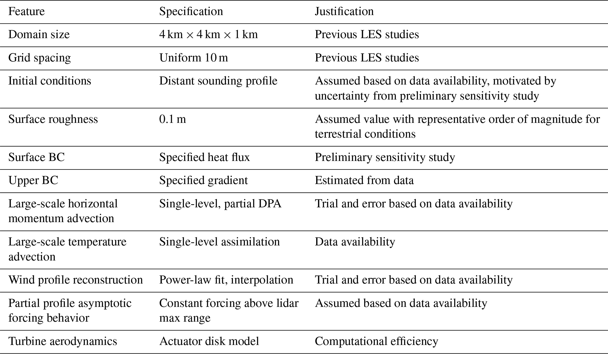
Table B1Summary of MMC modeling choices for horizontally homogeneous LES.
To model flow through a finite domain in the turbine simulation, the lateral boundary conditions were switched from periodic to a time-varying mixed inlet–outlet condition on the northern, western, and eastern boundaries – the southern boundary was assumed to have only outflow for the duration of the turbine simulation. On the mixed boundaries, each grid face is allowed to operate with inflow or outflow, determined by the sign of the instantaneous velocity flux. This mixed inflow–outflow condition therefore permits significant wind direction variations on a boundary with height and over time. The inflow boundary faces behave as a Dirichlet boundary condition with wind vectors and virtual potential temperatures set from time-varying boundary planes recorded from the precursor, whereas outflow boundary faces behave as a Neumann boundary condition with zero gradient. To maintain mass continuity, the fluxes on all outflow faces are scaled so that the total outflow exactly matches the total inflow. Dirichlet boundary data are updated at the same time intervals as the mesoscale forcing.
A summary of all MMC modeling choices is presented in Table B1. With the exception of the domain size, grid spacing, and surface roughness, all of the listed model features were varied and evaluated in the present work. The justification for these choices has been noted. For the turbine aerodynamics, actuator line modeling was also considered and is presented in Shaler et al. (2023).
The following steps were taken to reconstruct a full time–height history of wind speeds for MMC given limited field measurements (Fig. 5).
-
Quality control of measurements. Filter available lidar data by carrier-to-noise ratio (CNR; > −22.5 dB for this instrument) and greater than 50 % data availability. The threshold was chosen to be relatively low to provide more wind profile data during the daytime of this particular day. These quality-controlled data are shown in the left panel of Fig. 5.
-
Power-law wind profile approximation. Power-law wind speed profiles are calculated at 10 min intervals based on (i) sonic data alone, which provide high-frequency, high-quality measurements at two heights; (ii) all available met mast measurements, including the sonic anemometers and the cup anemometer (three heights); and (iii) all available measurements, which include met mast sensors and quality-controlled lidar data (between 3 and 10 heights, depending on lidar CNR). The shear exponent (α) is estimated from 10 min mean wind speed measurements, and the reference height in all three cases is taken to be the 50 m sonic anemometer measurement. The natural neighbor approach from Allaerts et al. (2023) was evaluated but was found to be sensitive to the spatiotemporal distribution of the wind data.
-
Quality control of approximate wind profiles. The instantaneous power-law profiles are filtered by the Pearson correlation coefficient (R2). While the sonic-only profiles have a perfect R2=1 for any U(z) that increases with height, R2<1 in general. At every instant, the power-law fit with R2 above a threshold of 0.9 with the highest number of data heights is selected. The conclusion of this step provides continuous wind profiles that increase monotonically with height up to the highest measurement height.
-
Vertical spline interpolation. When R2 is less than the threshold but lidar data are available up to the maximum range (180 m during the case day), these non-power-law-conforming or transient profiles are represented by piecewise cubic Hermite polynomials with . Near the surface, however, spline interpolation tended to underpredict the wind shear and overpredict wind speeds by approximately 1 m s−1 at the center of the first computational cell (5 m a.g.l.). As a workaround, the wind profile from the power-law fit with two sonic anemometer measurements, up to 50 m, was combined with the spline-interpolated profile between 50 and 180 m – spline extrapolation was not performed.
-
Linear interpolation. Linear interpolation was used to infill the profiles over time where neither a profile-law fit nor spline interpolation was performed. Above the highest measurement height, the wind is assumed to be constant. The final result is shown in the right panel of Fig. 5.
The time–height history of wind direction was generated in a more simplistic manner. Without an approximate profile (analogous to the power law for wind speeds), spline interpolation was applied between the lowest and highest available measurement. Wind directions at the surface and above the highest measurement were back and forward filled, respectively.
Evaluation of large-scale conditions using WRF NWP (model setup described in Table D1) showed sensitivity of the local wind speed, wind direction, and surface temperature to initial and boundary conditions derived from reanalysis data (Fig. D1). Reanalysis datasets considered included the US National Centers for Environmental Protection's Global Forecast System (GFS) final analysis, the European Centre for Medium-Range Weather Forecasts's fifth-generation reanalysis (ERA5), and the US National Aeronautics and Space Administration's Modern-Era Retrospective analysis for Research and Applications version 2 reanalysis (MERRA2). WRF mesoscale simulations were initialized from 26 December 2019 at 00:00 UTC, 25 December 2019 at 18:00 UTC, and 25 December 2019 at 12:00 UTC (hour 0, −6, and −12 of the case day, respectively) to assess the sensitivity to initial conditions. Lidar data become available during and following the evening transition.
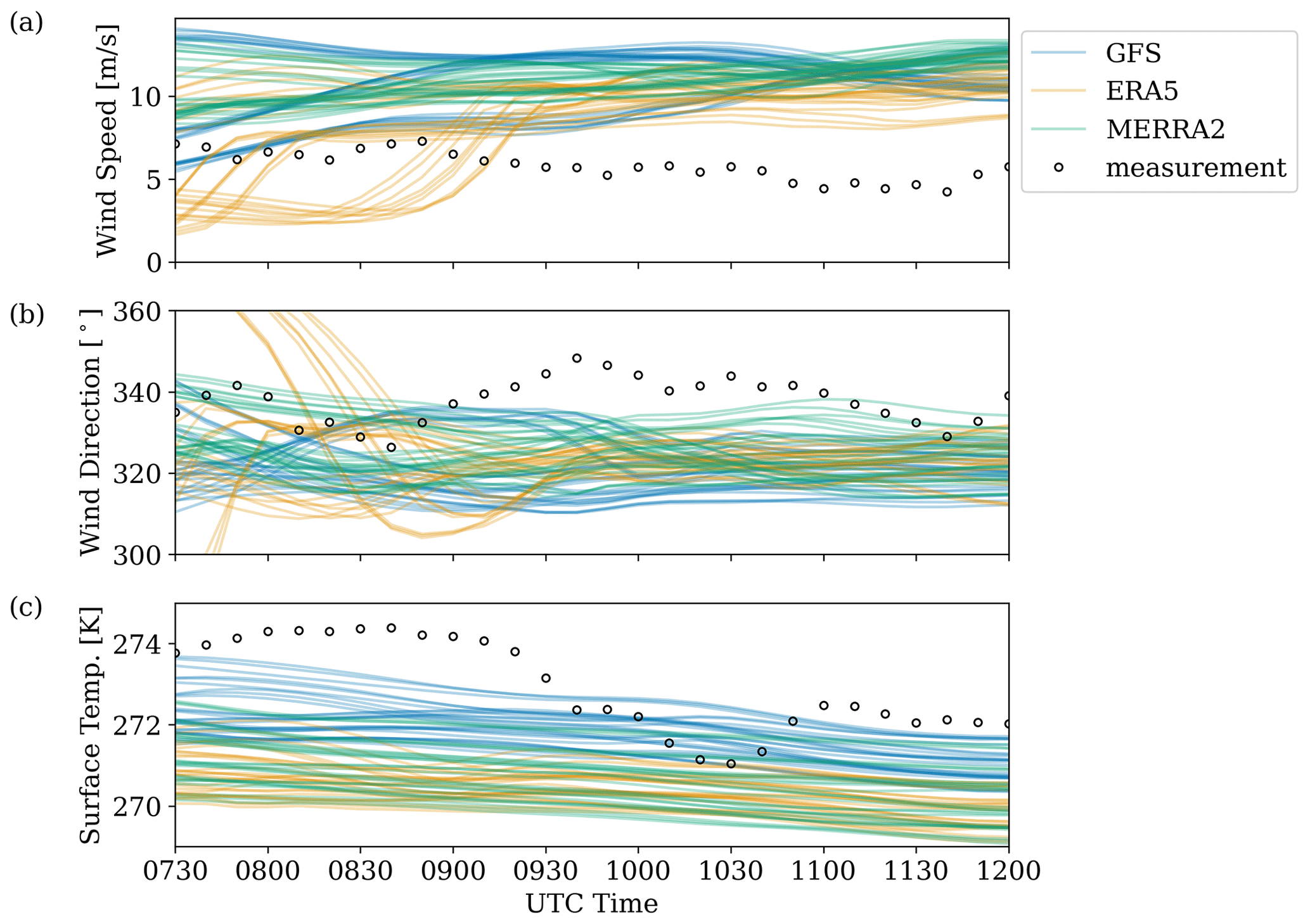
In all cases, the NWP model failed to capture locally observed atmospheric trends. The possibility that the mesoscale flow fields had a spatial offset was explored, i.e., that flow features were translated due to model deficiencies (e.g., inadequate terrain resolution). For a 3×3 subset of mesoscale grid points with 3 km spacing centered around turbine T2, ensembles of atmospheric quantities have been evaluated (Fig. D2). During the wake-steering period of interest, the mean wind speed generally had a non-negligible positive bias, the mean wind direction was biased towards the northwest, and temperatures were cold biased (Table D2). Modeled mesoscale data were therefore not used in this study.
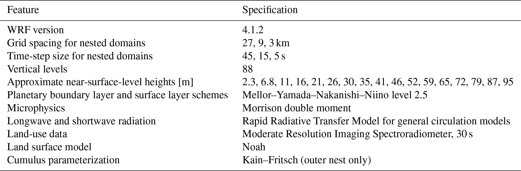
Table D2Summary of mean absolute error (MAE) and mean signed difference (MSD) for atmospheric state variables between 26 December 2019 at 07:30–12:00 UTC; ensembles include three simulation start times and nine sampling locations.
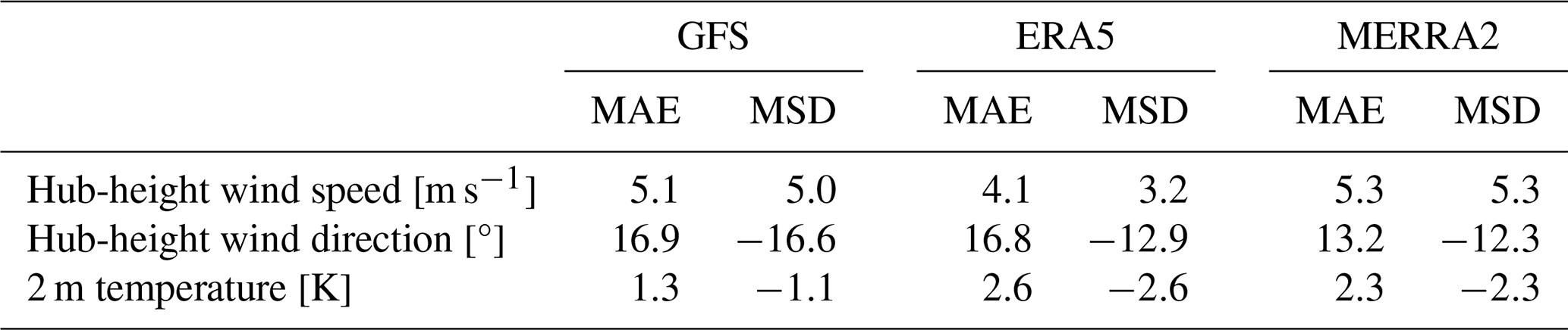
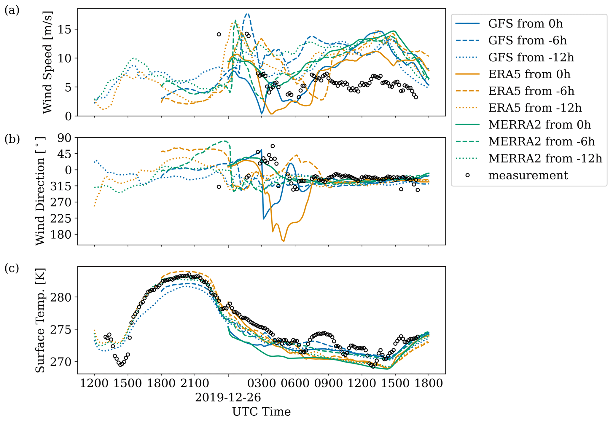
Figure D1WRF-simulated atmospheric conditions from virtual met masts near T2 given different initial and boundary conditions: hub-height wind speed (a) and direction (b), compared to lidar measurements; virtual temperature at 2 m a.g.l. (c), compared to met mast measurements.
The codes detailed in Appendix A are open-source and publicly available at https://github.com/NREL/SOWFA-6/tree/dev (Churchfield et al., 2021), https://github.com/OpenFAST/openfast (Jonkman et al., 2020), https://github.com/NREL/ROSCO (Abbas et al., 2020), and https://github.com/NREL/floris (Mudafort et al., 2020).
Currently, the data have not been made publicly available, per NREL's research agreement. However, if in the future portions of the data become available, this would be through the US Department of Energy's Wind Data Hub at https://a2e.energy.gov/about/dap (US Department of Energy, 2024).
The author has declared that there are no competing interests.
Publisher’s note: Copernicus Publications remains neutral with regard to jurisdictional claims made in the text, published maps, institutional affiliations, or any other geographical representation in this paper. While Copernicus Publications makes every effort to include appropriate place names, the final responsibility lies with the authors. The views expressed in the article do not necessarily represent the views of the DOE or the US Government. The US Government retains and the publisher, by accepting the article for publication, acknowledges that the US Government retains a nonexclusive, paid-up, irrevocable, worldwide license to publish or reproduce the published form of this work, or allow others to do so, for US Government purposes.
The author thanks the NREL instrumentation team that collected these experimental data, Chris Ivanov, Eric Simley, Jason Roadman, and Scott Dana; Mithu Debnath for providing the corrected lidar data; and Matthew Churchfield, Paula Doubrawa, and Jason Jonkman for supporting this effort through their respective projects.
This work was authored by the National Renewable Energy Laboratory, operated by the Alliance for Sustainable Energy, LLC, for the US Department of Energy (DOE) under contract no. DE-AC36-08GO28308. The research was performed using computational resources sponsored by the DOE's Office of Energy Efficiency and Renewable Energy and located at the National Renewable Energy Laboratory.
Funding was provided by the US Department of Energy Office of Energy Efficiency and Renewable Energy's Wind Energy Technologies Office (grant no. DE-AC36-08GO28308).
This paper was edited by Rebecca Barthelmie and reviewed by Javier Sanz Rodrigo and two anonymous referees.
Abbas, N., Zalkind, D., and Mudafort, R.: NREL's Reference OpenSource Controller (ROSCO) toolbox for wind turbine applications, version 2.0.2, GitHub [code], https://github.com/NREL/ROSCO (last access: 7 July 2020), 2020. a
Abbas, N. J., Zalkind, D. S., Pao, L., and Wright, A.: A Reference Open-Source Controller for Fixed and Floating Offshore Wind Turbines, Wind Energ. Sci., 7, 53–73, https://doi.org/10.5194/wes-7-53-2022, 2022. a
Abkar, M., Sharifi, A., and Porté-Agel, F.: Wake Flow in a Wind Farm during a Diurnal Cycle, J. Turbul., 17, 420–441, https://doi.org/10.1080/14685248.2015.1127379, 2016. a
Allaerts, D., Quon, E., and Churchfield, M.: Using Observational Mean-flow Data to Drive Large-eddy Simulations of a Diurnal Cycle at the SWiFT Site, Wind Energy, 26, 469–492, https://doi.org/10.1002/we.2811, 2023. a, b, c, d, e, f
Allaerts, D. J. N., Quon, E., Draxl, C., and Churchfield, M.: Development of a Time–Height Profile Assimilation Technique for Large-Eddy Simulation, Bound.-Lay. Meteorol., 176, 2533–2550, https://doi.org/10.1007/s10546-020-00538-5, 2020. a, b, c, d, e, f, g, h
Angevine, W. M., Edwards, J. M., Lothon, M., LeMone, M. A., and Osborne, S. R.: Transition Periods in the Diurnally-Varying Atmospheric Boundary Layer Over Land, Bound.-Lay. Meteorol., 177, 205–223, https://doi.org/10.1007/s10546-020-00515-y, 2020. a
Arthur, R. S., Mirocha, J. D., Marjanovic, N., Hirth, B. D., Schroeder, J. L., Wharton, S., and Chow, F. K.: Multi-Scale Simulation of Wind Farm Performance during a Frontal Passage, Atmosphere, 11, 245, https://doi.org/10.3390/atmos11030245, 2020. a, b
Basu, S., Holtslag, A. A. M., Wiel, B. J. H. V. D., Moene, A. F., and Steeneveld, G.-J.: An Inconvenient “Truth” about Using Sensible Heat Flux as a Surface Boundary Condition in Models under Stably Stratified Regimes, Acta Geophys., 56, 88–99, https://doi.org/10.2478/s11600-007-0038-y, 2008a. a
Basu, S., Vinuesa, J.-F., and Swift, A.: Dynamic LES Modeling of a Diurnal Cycle, Journal of Applied Meteorology and Climatology, 47, 1156–1174, https://doi.org/10.1175/2007JAMC1677.1, 2008b. a
Berg, L. K., Liu, Y., Yang, B., Qian, Y., Olson, J., Pekour, M., Ma, P.-L., and Hou, Z.: Sensitivity of Turbine-Height Wind Speeds to Parameters in the Planetary Boundary-Layer Parametrization Used in the Weather Research and Forecasting Model: Extension to Wintertime Conditions, Bound.-Lay. Meteorol., 170, 507–518, https://doi.org/10.1007/s10546-018-0406-y, 2019. a
Bosveld, F. C., Baas, P., Steeneveld, G.-J., Holtslag, A. A. M., Angevine, W. M., Bazile, E., de Bruijn, E. I. F., Deacu, D., Edwards, J. M., Ek, M., Larson, V. E., Pleim, J. E., Raschendorfer, M., and Svensson, G.: The Third GABLS Intercomparison Case for Evaluation Studies of Boundary-Layer Models. Part B: Results and Process Understanding, Bound.-Lay. Meteorol., 152, 157–187, https://doi.org/10.1007/s10546-014-9919-1, 2014a. a
Bosveld, F. C., Baas, P., van Meijgaard, E., de Bruijn, E. I. F., Steeneveld, G.-J., and Holtslag, A. A. M.: The Third GABLS Intercomparison Case for Evaluation Studies of Boundary-Layer Models. Part A: Case Selection and Set-Up, Bound.-Lay. Meteorol., 152, 133–156, https://doi.org/10.1007/s10546-014-9917-3, 2014b. a
Branlard, E. and Meyer Forsting, A. R.: Assessing the Blockage Effect of Wind Turbines and Wind Farms Using an Analytical Vortex Model, Wind Energy, 23, 2068–2086, https://doi.org/10.1002/we.2546, 2020. a
Churchfield, M., Thedin, R., Quon, E., Vijayakumar, G., Benito, P., and Doekemeijer, B.: Simulator fOr Wind Farm Applications, GitHub [code], https://github.com/NREL/SOWFA-6/tree/dev (last accesse: 4 December 2021), 2021. a
Churchfield, M. J., Lee, S., Michalakes, J., and Moriarty, P. J.: A Numerical Study of the Effects of Atmospheric and Wake Turbulence on Wind Turbine Dynamics, J. Turbul., 13, 1–32, https://doi.org/10.1080/14685248.2012.668191, 2012. a
Deardorff, J. W.: Stratocumulus-Capped Mixed Layers Derived from a Three-Dimensional Model, Bound.-Lay. Meteorol., 18, 495–527, 1980. a
Doekemeijer, B. M., Simley, E., and Fleming, P.: Comparison of the Gaussian Wind Farm Model with Historical Data of Three Offshore Wind Farms, Energies, 15, 1964, https://doi.org/10.3390/en15061964, 2022. a
Draxl, C., Allaerts, D., Quon, E., and Churchfield, M.: Coupling Mesoscale Budget Components to Large-Eddy Simulations for Wind-Energy Applications, Bound.-Lay. Meteorol., 179, 73–98, https://doi.org/10.1007/s10546-020-00584-z, 2021. a
Duynkerke, P. G., de Roode, S. R., van Zanten, M. C., Calvo, J., Cuxart, J., Cheinet, S., Chlond, A., Grenier, H., Jonker, P. J., Köhler, M., Lenderink, G., Lewellen, D., Lappen, C.-L., Lock, A. P., Moeng, C.-H., Müller, F., Olmeda, D., Piriou, J.-M., Sánchez, E., and Sednev, I.: Observations and Numerical Simulations of the Diurnal Cycle of the EUROCS Stratocumulus Case, Q. J. Roy. Meteorol. Soc., 130, 3269–3296, https://doi.org/10.1256/qj.03.139, 2004. a
Fleming, P., King, J., Dykes, K., Simley, E., Roadman, J., Scholbrock, A., Murphy, P., Lundquist, J. K., Moriarty, P., Fleming, K., van Dam, J., Bay, C., Mudafort, R., Lopez, H., Skopek, J., Scott, M., Ryan, B., Guernsey, C., and Brake, D.: Initial Results from a Field Campaign of Wake Steering Applied at a Commercial Wind Farm – Part 1, Wind Energ. Sci., 4, 273–285, https://doi.org/10.5194/wes-4-273-2019, 2019. a, b, c
Fleming, P., King, J., Simley, E., Roadman, J., Scholbrock, A., Murphy, P., Lundquist, J. K., Moriarty, P., Fleming, K., van Dam, J., Bay, C., Mudafort, R., Jager, D., Skopek, J., Scott, M., Ryan, B., Guernsey, C., and Brake, D.: Continued Results from a Field Campaign of Wake Steering Applied at a Commercial Wind Farm – Part 2, Wind Energ. Sci., 5, 945–958, https://doi.org/10.5194/wes-5-945-2020, 2020. a, b, c
Hannesdóttir, Á., Kelly, M., and Dimitrov, N.: Extreme Wind Fluctuations: Joint Statistics, Extreme Turbulence, and Impact on Wind Turbine Loads, Wind Energ. Sci., 4, 325–342, https://doi.org/10.5194/wes-4-325-2019, 2019. a
Haupt, S., Berg, L., Decastro, A., Gagne, D., Jimenez, P., Juliano, T., Kosovic, B., Quon, E., Shaw, W., Churchfield, M., Draxl, C., Hawbecker, P., Jonko, A., Kaul, C., Mirocha, J., and Rai, R.: Outcomes of the DOE Workshop on Atmospheric Challenges for the Wind Energy Industry, Tech. Rep. PNNL–30828, 1762812, OSTI.GOV, https://doi.org/10.2172/1762812, 2020. a, b
Haupt, S. E., Kosovic, B., Shaw, W., Berg, L. K., Churchfield, M., Cline, J., Draxl, C., Ennis, B., Koo, E., Kotamarthi, R., Mazzaro, L., Mirocha, J., Moriarty, P., Muñoz-Esparza, D., Quon, E., Rai, R. K., Robinson, M., and Sever, G.: On Bridging a Modeling Scale Gap: Mesoscale to Microscale Coupling for Wind Energy, B. Am. Meteorol. Soc., 100, 2533–2550, https://doi.org/10.1175/BAMS-D-18-0033.1, 2019. a, b
Haupt, S. E., Kosović, B., Berg, L. K., Kaul, C. M., Churchfield, M., Mirocha, J., Allaerts, D., Brummet, T., Davis, S., DeCastro, A., Dettling, S., Draxl, C., Gagne, D. J., Hawbecker, P., Jha, P., Juliano, T., Lassman, W., Quon, E., Rai, R. K., Robinson, M., Shaw, W., and Thedin, R.: Lessons Learned in Coupling Atmospheric Models across Scales for Onshore and Offshore Wind Energy, Wind Energ. Sci., 8, 1251–1275, https://doi.org/10.5194/wes-8-1251-2023, 2023. a, b
Howland, M. F., Ghate, A. S., Quesada, J. B., Pena Martínez, J. J., Zhong, W., Larrañaga, F. P., Lele, S. K., and Dabiri, J. O.: Optimal Closed-Loop Wake Steering – Part 2: Diurnal Cycle Atmospheric Boundary Layer Conditions, Wind Energ. Sci., 7, 345–365, https://doi.org/10.5194/wes-7-345-2022, 2022. a
Jayaraman, B., Quon, E., Li, J., and Chatterjee, T.: Structure of Offshore Low-Level Jet Turbulence and Implications to Mesoscale-to-Microscale Coupling, J. Phys.: Conf. Ser., 2265, 022064, https://doi.org/10.1088/1742-6596/2265/2/022064, 2022. a, b
Jiménez, P. A. and Dudhia, J.: On the Ability of the WRF Model to Reproduce the Surface Wind Direction over Complex Terrain, J. Appl. Meteorol. Clim., 52, 1610–1617, https://doi.org/10.1175/JAMC-D-12-0266.1, 2013. a
Jonkman, B., Mudafort, R., Platt, A., Branlard, E., et al.: OpenFAST version 2.4.0, GitHub [code], https://github.com/OpenFAST/openfast (last access: 9 December 2020), 2020. a
King, J., Fleming, P., King, R., Martínez-Tossas, L. A., Bay, C. J., Mudafort, R., and Simley, E.: Control-Oriented Model for Secondary Effects of Wake Steering, Wind Energ. Sci., 6, 701–714, https://doi.org/10.5194/wes-6-701-2021, 2021. a
Kleczek, M. A., Steeneveld, G.-J., and Holtslag, A. A. M.: Evaluation of the Weather Research and Forecasting Mesoscale Model for GABLS3: Impact of Boundary-Layer Schemes, Boundary Conditions and Spin-Up, Bound.-Lay. Meteorol., 152, 213–243, https://doi.org/10.1007/s10546-014-9925-3, 2014. a
Kumar, V., Kleissl, J., Meneveau, C., and Parlange, M. B.: Large-Eddy Simulation of a Diurnal Cycle of the Atmospheric Boundary Layer: Atmospheric Stability and Scaling Issues: LES Of A Diurnal Cycle Of The ABL, Water Resour. Res., 42, 1496–1516, https://doi.org/10.1029/2005WR004651, 2006. a, b
Kumar, V., Svensson, G., Holtslag, A. A. M., Meneveau, C., and Parlange, M. B.: Impact of Surface Flux Formulations and Geostrophic Forcing on Large-Eddy Simulations of Diurnal Atmospheric Boundary Layer Flow, J. Appl. Meteorol. Clim., 49, 1496–1516, https://doi.org/10.1175/2010JAMC2145.1, 2010. a, b
Lignarolo, L. E., Mehta, D., Stevens, R. J., Yilmaz, A. E., van Kuik, G., Andersen, S. J., Meneveau, C., Ferreira, C. J., Ragni, D., Meyers, J., van Bussel, G. J., and Holierhoek, J.: Validation of Four LES and a Vortex Model against Stereo-PIV Measurements in the near Wake of an Actuator Disc and a Wind Turbine, Renew. Energy, 94, 510–523, https://doi.org/10.1016/j.renene.2016.03.070, 2016. a
Liu, Y., Bourgeois, A., Warner, T., and Swerdlin, S.: An “Observation-Nudging”-Based FDDA Scheme for WRF-ARW for Mesoscale Data Assimilation and Forecasting, in: 4th Symposium on Space Weather, 15 January 2007, San Antonio, Texas, p. 6, https://ams.confex.com/ams/87ANNUAL/webprogram/Paper118226.html (last access: 28 February 2024), 2007. a
Meyers, J., Bottasso, C., Dykes, K., Fleming, P., Gebraad, P., Giebel, G., Göçmen, T., and van Wingerden, J.-W.: Wind Farm Flow Control: Prospects and Challenges, Wind Energ. Sci., 7, 2271–2306, https://doi.org/10.5194/wes-7-2271-2022, 2022. a
Mirocha, J. D., Rajewski, D. A., Marjanovic, N., Lundquist, J. K., Kosović, B., Draxl, C., and Churchfield, M. J.: Investigating Wind Turbine Impacts on Near-Wake Flow Using Profiling Lidar Data and Large-Eddy Simulations with an Actuator Disk Model, J. Renew. Sustain. Energ., 7, 043143, https://doi.org/10.1063/1.4928873, 2015. a
Mudafort, R., Fleming, P., Bay, C., Hammond, R., et al.: FLORIS Wake Modeling and Wind Farm Controls Software, version 2.0.0, GitHub [code], https://github.com/NREL/floris (last access: 12 June 2020), 2020. a
Neunaber, I., Hölling, M., Whale, J., and Peinke, J.: Comparison of the Turbulence in the Wakes of an Actuator Disc and a Model Wind Turbine by Higher Order Statistics: A Wind Tunnel Study, Renew. Energy, 179, 1650–1662, https://doi.org/10.1016/j.renene.2021.08.002, 2021. a
NREL: OpenFAST, Version 2.4.0, GitHub [code], https://github.com/OpenFAST/openfast (last access: 9 December 2020), 2020. a
Porté-Agel, F.: Wind-Turbine and Wind-Farm Flows: A Review, Bound.-Lay. Meteorol., 174, 1–59, https://doi.org/10.1007/s10546-019-00473-0, 2020. a
Rai, R. K., Berg, L. K., Kosović, B., Haupt, S. E., Mirocha, J. D., Ennis, B. L., and Draxl, C.: Evaluation of the Impact of Horizontal Grid Spacing in Terra Incognita on Coupled Mesoscale–Microscale Simulations Using the WRF Framework, Mon. Weather Rev., 147, 1007–1027, https://doi.org/10.1175/MWR-D-18-0282.1, 2019. a
Revaz, T. and Porté-Agel, F.: Large-Eddy Simulation of Wind Turbine Flows: A New Evaluation of Actuator Disk Models, Energies, 14, 3745, https://doi.org/10.3390/en14133745, 2021. a, b
Santoni, C., García-Cartagena, E. J., Ciri, U., Zhan, L., Valerio Iungo, G., and Leonardi, S.: One-Way Mesoscale-Microscale Coupling for Simulating a Wind Farm in North Texas: Assessment against SCADA and LiDAR Data, Wind Energy, 23, 691–710, https://doi.org/10.1002/we.2452, 2020. a
Santos, R., van Dam, J., and Santos Wind Engineering Technologies, Inc., Portland, Maine: Mechanical Loads Test Report for the U.S. Department of Energy 1.5-Megawatt Wind Turbine, Tech. Rep. NREL/TP–5000-63679, 1215119, NREL, https://doi.org/10.2172/1215119, 2015. a
Sanz Rodrigo, J., Allaerts, D., Avila, M., Barcons, J., Cavar, D., Arroyo, R. C., Churchfield, M., Kosovic, B., JK Lundquist, Meyers, J., Esparza, D. M., Palma, J. M. L. M., Tomaszewski, J. M., Troldborg, N., van der Laan, M. P., and Rodrigues, C. V.: Results of the GABLS3 Diurnal-Cycle Benchmark for Wind Energy Applications, J. Phys.: Conf. Ser., 854, 012037, https://doi.org/10.1088/1742-6596/854/1/012037, 2017a. a
Sanz Rodrigo, J., Chávez Arroyo, R. A., Moriarty, P., Churchfield, M., Kosović, B., Réthoré, P.-E., Hansen, K. S., Hahmann, A., Mirocha, J. D., and Rife, D.: Mesoscale to Microscale Wind Farm Flow Modeling and Evaluation, WIREs Energ. Environ., 6, e214, https://doi.org/10.1002/wene.214, 2017b. a
Sanz Rodrigo, J., Santos, P., Chávez Arroyo, R., Avila, M., Cavar, D., Lehmkuhl, O., Owen, H., Li, R., and Tromeur, E.: The ALEX17 Diurnal Cycles in Complex Terrain Benchmark, J. Phys.: Conf. Ser., 1934, 012002, https://doi.org/10.1088/1742-6596/1934/1/012002, 2021. a
Schalkwijk, J., Jonker, H. J. J., Siebesma, A. P., and Bosveld, F. C.: A Year-Long Large-Eddy Simulation of the Weather over Cabauw: An Overview, Mon. Weather Rev., 143, 828–844, https://doi.org/10.1175/MWR-D-14-00293.1, 2015. a
Schumann, U.: Subgrid Scale Model for Finite Difference Simulations of Turbulent Flows in Plane Channels and Annuli, J. Comput. Phys., 18, 376–404, https://doi.org/10.1016/0021-9991(75)90093-5, 1975. a
Shaler, K., Quon, E., Ivanov, H., and Jonkman, J.: Wind Farm Structural Response and Wake Dynamics for an Evolving Stable Boundary Layer: Computational and Experimental Comparisons, Wind Energ. Sci. Discuss. [preprint], https://doi.org/10.5194/wes-2023-138, in review, 2023. a, b, c, d
Shapiro, C. R., Starke, G. M., and Gayme, D. F.: Turbulence and Control of Wind Farms, Annu. Rev. Control Robot. Autonom. Syst., 5, 579–602, https://doi.org/10.1146/annurev-control-070221-114032, 2022. a
Simisiroglou, N., Breton, S.-P., and Ivanell, S.: Validation of the Actuator Disc Approach Using Small-Scale Model Wind Turbines, Wind Energ. Sci., 2, 587–601, https://doi.org/10.5194/wes-2-587-2017, 2017. a
Simley, E., Fleming, P., and King, J.: Design and Analysis of a Wake Steering Controller with Wind Direction Variability, Wind Energ. Sci., 5, 451–468, https://doi.org/10.5194/wes-5-451-2020, 2020. a
Stauffer, D. R. and Seaman, N. L.: Multiscale Four-Dimensional Data Assimilation, J. Appl. Meteorol., 33, 416–434, https://doi.org/10.1175/1520-0450(1994)033<0416:MFDDA>2.0.CO;2, 1994. a
Stoll, R., Gibbs, J. A., Salesky, S. T., Anderson, W., and Calaf, M.: Large-Eddy Simulation of the Atmospheric Boundary Layer, Bound.-Lay. Meteorol., 177, 541–581, https://doi.org/10.1007/s10546-020-00556-3, 2020. a, b
Sun, J., Lenschow, D. H., Burns, S. P., Banta, R. M., Newsom, R. K., Coulter, R., Frasier, S., Ince, T., Nappo, C., Balsley, B. B., Jensen, M., Mahrt, L., Miller, D., and Skelly, B.: Atmospheric Disturbances That Generate Intermittent Turbulence in Nocturnal Boundary Layers, Bound.-Lay. Meteorol., 110, 255–279, https://doi.org/10.1023/A:1026097926169, 2004. a
Telford, P. J., Braesicke, P., Morgenstern, O., and Pyle, J. A.: Technical Note: Description and Assessment of a Nudged Version of the New Dynamics Unified Model, Atmos. Chem. Phys., 8, 1701–1712, https://doi.org/10.5194/acp-8-1701-2008, 2008. a
US Department of Energy Atmosphere to Electrons: Wind Data Hub, https://a2e.energy.gov/about/dap (last access: 28 February 2024), 2024. a
Vollmer, L., Lee, J. C.-Y., Steinfeld, G., and Lundquist, J. K.: A Wind Turbine Wake in Changing Atmospheric Conditions: LES and Lidar Measurements, J. Phys.: Conf. Ser., 854, 012050, https://doi.org/10.1088/1742-6596/854/1/012050, 2017a. a
Vollmer, L., Steinfeld, G., and Kühn, M.: Transient LES of an Offshore Wind Turbine, Wind Energ. Sci., 2, 603–614, https://doi.org/10.5194/wes-2-603-2017, 2017b. a, b
Xu, H. H. A. and Yang, X. I. A.: Treatment of Unphysical Numerical Oscillations via Local Grid Refinement, Phys. Fluids, 33, 077104, https://doi.org/10.1063/5.0054642, 2021. a
Yang, B., Qian, Y., Berg, L. K., Ma, P.-L., Wharton, S., Bulaevskaya, V., Yan, H., Hou, Z., and Shaw, W. J.: Sensitivity of Turbine-Height Wind Speeds to Parameters in Planetary Boundary-Layer and Surface-Layer Schemes in the Weather Research and Forecasting Model, Bound.-Lay. Meteorol., 162, 117–142, https://doi.org/10.1007/s10546-016-0185-2, 2017. a
Zajaczkowski, F. J., Haupt, S. E., and Schmehl, K. J.: A Preliminary Study of Assimilating Numerical Weather Prediction Data into Computational Fluid Dynamics Models for Wind Prediction, J. Wind Eng. Indust. Aerodynam., 99, 320–329, https://doi.org/10.1016/j.jweia.2011.01.023, 2011. a
- Abstract
- Copyright statement
- Introduction
- Field campaign
- Meteorological considerations
- A tailored mesoscale-to-microscale coupling approach
- Results and discussion
- Conclusions
- Appendix A: Simulation codes used
- Appendix B: Large-eddy simulation setup
- Appendix C: Wind field reconstruction
- Appendix D: Preliminary mesoscale simulations
- Code availability
- Data availability
- Competing interests
- Disclaimer
- Acknowledgements
- Financial support
- Review statement
- References