Modeling frontal low-level jets and associated extreme wind power ramps over the North Sea

The increasing global demand for wind power underscores the importance of understanding and characterizing extreme ramp events, which are significant fluctuations in wind power generation over short periods that pose challenges for grid integration. This study focuses on modeling frontal low-level jets (FLLJs) and associated extreme ramp-down events, particularly their impact on wind power production at Belgium offshore wind farms. Using the Weather Research and Forecasting (WRF) model, we analyzed five cases of extreme wind power ramp-down events, including in-depth analysis of two cases and generalization of three additional cases. We assessed the sensitivity of various model configurations, including initial and boundary condition (IC/BC) datasets (ERA5 and CERRA), the activation of Fitch wind farm parameterization (WFP), planetary boundary layer (PBL) schemes, and single- versus nested-domain configuration. Our findings indicate that CERRA IC/BCs provide a superior representation of atmospheric flow compared to ERA5, resulting in more accurate predictions of ramp timing, intensity, and FLLJ characteristics. The WFP significantly impacts wind power output by modeling turbine interactions and wake effects, leading to slightly lower wind speeds. The scale-aware Shin and Hong PBL scheme yielded a stronger FLLJ core at higher altitudes with a more pronounced jet nose, although wind speeds below 200 m were lower compared to the Mellor–Yamada–Nakanishi–Niino 2.5 scheme. Single-domain configuration proved more effective in simulating wind power ramps but had higher core heights and higher wind speeds below 200 m, resulting in a diffused jet profile. Our analysis highlights that reliable simulation of extreme ramps associated with FLLJs using a single-domain configuration could reduce computational costs. Further, the FLLJs and associated extreme ramps can be predicted 1 d in advance, offering substantial benefits for operational efficiency in wind energy management.

1 Introduction

The demand for global wind power is surging as renewable energy is increasingly seen as essential to combat climate change. The European Union aims for 32 % renewable energy by 2030 to reduce greenhouse gas emissions by at least 55 % (European Union, 2018). Offshore wind farms (OWFs) are pivotal in meeting these goals, despite their higher construction and maintenance costs compared to onshore wind farms (Zheng et al., 2016). This is due to two main factors: the higher capacity factor of OWFs, as offshore winds are generally 25 % stronger and can be utilized 2–3 times longer than onshore winds (Tambke et al., 2005), and technological advancements that allow for the use of larger, more efficient turbines (Mehta et al., 2024). By 2019, Europe's OWF capacity reached 22 GW, with 77 % located in the North Sea. The EU plans to expand offshore wind capacity to 450 GW by 2050, with 47 % (212 GW) in the North Sea, necessitating an annual consenting rate of 8.8 GW (Wind Europe, 2019). This makes the North Sea a critical area for OWF development.

A major challenge for integrating large-scale wind power into the grid is managing extreme ramp events, which are significant fluctuations in wind power generation over short periods (Ueckerdt et al., 2015; Mararakanye and Bekker, 2019). Without large-scale energy storage, power production must match power consumption, a balance maintained by transmission system operators (TSOs). Often, ramp-up events necessitate wind farm curtailment because surplus electricity cannot be dispatched, leading to profit loss for farm owners. At other times, when wind power output suddenly increases, conventional power generation, such as coal and natural gas, must reduce output, a process known as cycling (Veron et al., 2018). This cycling lowers the capacity credit of conventional generation. In a more complex manner, during ramp-down events, when wind power output suddenly drops, the supply from conventional power generators must increase to meet demand. TSOs often purchase these resources in competitive markets at high rates. In critical situations, load shedding becomes necessary due to minimal power output from wind farms. Wind farm owners then incur additional costs when they fail to meet specific loads and quotas (Valldecabres et al., 2020).

These challenges were evident in the case of Great Britain offshore wind farms on 3 November 2014 (Drew et al., 2017). During that day, wind power output increased by 1.1 GW in 2 h and 45 min (ramp-up), followed by a 1.2 GW decrease in 1 h and 50 min (ramp-down). Analysis of the meteorological conditions has shown that the ramp-up was caused by a trough that formed behind a large weather front, while the ramp-down was caused by the subsidence of the trough. This unforecasted event caused a market surplus of 570 MWh at 15:30 UTC due to unexpected generation in the Thames Estuary and a deficit of 820 MWh at 17:00 UTC due to the sudden drop in generation. The imbalance coincided with high demand, leaving fewer available generation units. Expensive short-term operating reserves were deployed, causing a system buy price spike to GBP 183 per megawatt-hour, the 16th highest price of the year. This event underscores the importance of a comprehensive understanding of power ramp events and the atmospheric phenomena that contribute to their occurrence.

Ramp-up events are primarily caused by synoptic-scale weather phenomena, such as cyclones (Lacerda et al., 2017; Drew et al., 2018) and cold fronts (Cutler et al., 2007; Linden et al., 2012; Cheng et al., 2013; Haupt et al., 2014; Marjanovic et al., 2014; Pichault et al., 2021; Pereyra-Castro and Caetano, 2022; Arthur et al., 2020; Veron et al., 2018). These events can also be triggered by mesoscale phenomena, such as thunderstorms (Hawbecker et al., 2017; Cheng et al., 2013; Drew et al., 2018; Pichault et al., 2021) and low-level jets (Freedman et al., 2008). Conversely, ramp-down events occur due to a decrease in wind speed, often triggered by the relaxation of cold fronts (Drew et al., 2018; Zhao et al., 2019; Dalton et al., 2019) and the passage of warm fronts (Cheneka et al., 2021). Practically, ramp-down events pose a greater problem than ramp-up events, primarily due to the significant penalties that wind farm owners may incur from short supply. Additionally, ramp-down events can lead to a decrease in system frequency (Ela and Kirby, 2008).

Gallego-Castillo et al. (2015) pointed out the importance of modeling and understanding the causative meteorological phenomena of extreme ramps, which would help improve ramp forecasting frameworks. Our paper focuses on modeling one such weather phenomenon called the frontal low-level jet (FLLJ) associated with cold fronts, which tends to cause extreme wind power ramp-down events, using the Weather Research and Forecasting (WRF) model.

Previous studies, such as Freedman et al. (2008), suggested that a gradual rather than a sharp decline in wind speed is more common during cold fronts, making up-ramps more frequent than down-ramps. This is evidenced by a large number of studies focused on ramp-up events associated with cold fronts. However, the FLLJ causes an abrupt wind speed drop that triggers an extreme ramp-down event on a timescale of 15 to 60 min, which is a unique flow feature we report in the present study. To the best of our knowledge, there are no peer-reviewed journal articles associating FLLJs with extreme wind power ramp-down events. However, there was a study from our group, presented as a non-peer-reviewed master's thesis work (Dreef, 2019), which conducted some very preliminary cases in Scotland. That prompted a detailed investigation that led to this particular work.

Larger, synoptically driven features have longer timescales and are theoretically more straightforward to model and forecast than local-scale phenomena, which usually require fine-scale information about land-surface conditions and turbulent mixing in the atmosphere (Marjanovic et al., 2014). The FLLJ, though primarily a synoptic-scale phenomenon, also consists of local-scale features along with their intensity and temporal evolution in specific regions. Thus, while synoptic-scale characteristics are expected to be modeled with relative accuracy, the local-scale features exhibit significant sensitivity to model physics parameterizations, domain configuration, and the resolution of the forcing data (Storm et al., 2009; Nunalee and Basu, 2014; Aird et al., 2021; Tay et al., 2021; Larsén and Fischereit, 2021; Wagner et al., 2019).

As a first step towards a better understanding, we investigate the modeling efforts of extreme wind ramp-down events associated with FLLJs and their impact on wind power production, using the WRF model (Skamarock et al., 2019). In the mesoscale modeling community, it is well known that forcing data significantly influence simulation accuracy (Carvalho et al., 2014; de Linaje et al., 2019; Hahmann et al., 2020). Nonetheless, the fifth-generation ECMWF atmospheric reanalysis (ERA5) (Hersbach et al., 2020), existing at a ∼ 32 km resolution, has been the preferred forcing data in wind resource modeling (Olauson, 2018; Ramon et al., 2019; Gualtieri, 2022). However, a recent development in meteorological reanalysis is the Copernicus Regional Reanalysis for Europe (CERRA) (Schimanke et al., 2021; Ridal et al., 2024), offering a significantly improved resolution of 5.5 km. Despite the advantages of CERRA, the data have never been used as forcing data in wind resource modeling. Therefore, the present study aims to capitalize on the capabilities of CERRA data as initial and boundary conditions. The improved resolution of CERRA forcing data makes it possible for such modeling, with a detailed representation of atmospheric processes and less computational resource utilization. In addition, since the FLLJ is an atmospheric boundary layer phenomenon, the model accuracy will be more sensitive to the use of appropriate planetary boundary layer (PBL) parameterization (Nunalee and Basu, 2014; Gevorgyan, 2018; Vemuri et al., 2022). The WRF model has the capability to parameterize the interaction of wind turbines with atmospheric flow through a wind farm parameterization (WFP). However, in the absence of wind farm specifications, it is necessary to understand to what extent the WFP contributes to the modeling accuracy.

Keeping these modeling parameters in mind, we aim to determine how well the FLLJ and the associated ramp-down event can be modeled and assess their impact on wind power production at the Belgium offshore wind farm. We also seek to evaluate the sensitivity of ramp characteristics in terms of timing and intensity, as well as the FLLJ characteristics in terms of core strength and height, to the choice of forcing data, PBL schemes, WFP, and domain configuration.

The organization of this paper is as follows. Section 2 briefly discusses the meteorological background of the FLLJ. The methods used here are introduced in Sect. 3, including the data, a description of two case studies, a diverse set of WRF model configurations, and the simulation setup. The results are presented in Sect. 4. The conclusions and the future scope are presented in Sect. 5. The Appendix consists of additional information, including a description of three additional case studies identified for modeling, a comparison between ERA5 and CERRA forcing data, and an illustration of some additional results.

2 Frontal low-level jet: a meteorological perspective

A low-level jet (LLJ) is a local maximum in the vertical wind speed profile, often referred to as a core or sometimes a nose, characterized by a modest (approximately 2–3 m s⁻¹) decrease in wind speed above and below the core. LLJs typically occur within the planetary boundary layer (Bonner, 1968; Hallgren et al., 2023). They can be induced by various mechanisms, including inertial oscillation (Blackadar, 1957; Bonner, 1968); diurnal changes related to surface and terrain characteristics, such as coastal jets (Smedman et al., 1993, 1995; Nunalee and Basu, 2014); large-scale baroclinicity influenced by sloping terrain (Xing-Sheng et al., 1983; Gerber et al., 1989); and geostrophic adjustment, as seen in barrier jets (Parish and Oolman, 2010; Li and Chen, 1998).

The frontal low-level jet (FLLJ) shares similarities with the barrier jet mechanism. Observations by Browning and Harrold (1970) first identified the FLLJ while studying air circulation and precipitation growth in cold fronts over the British Isles. They reported strong wind speeds, ranging from 25 to 30 m s⁻¹, just ahead of cold frontal surfaces. Subsequent research has confirmed the existence and characteristics of FLLJs (Browning and Pardoe, 1973; Browning, 1974; Browning and Monk, 1982; Browning, 1986; Browning et al., 1998; Orlanski and Ross, 1977; Thorpe and Clough, 1991; Kotroni and Lagouvardos, 1993; Uccellini and Johnson, 1979; Brill et al., 1985; Dudhia, 1993; Chen et al., 1994; Wakimoto and Murphey, 2008; Demirdjian et al., 2020; Tay et al., 2021). The key characteristics of the FLLJ are as follows:

• It is a band of strong winds with velocities ranging from 25 to 30 m s⁻¹, typically located within the 900–850 mb pressure level, and forms ahead of a cold frontal surface.

• It is a synoptic-scale phenomenon that extends several hundred kilometers ahead of the frontal surface.

• The jet's acceleration is driven by the isallobaric term, while the Coriolis torque and advective tendency terms influence its propagation along the frontal surface and adjust its alignment relative to the frontal boundary.

• An important feature of the FLLJ is the abrupt wind speed drop immediately following the jet, which is accompanied by a significant change in wind direction.

The intense wind speed during the FLLJ, combined with the drastic decrease in wind speed that follows, results in extreme ramp-down events.

Despite its well-documented characteristics, there is a notable lack of modeling studies focused on the influence of FLLJs and associated extreme ramp-down events on wind power production. While the basic characteristics of FLLJs are known, detailed knowledge regarding their impact on extreme ramps and wind energy production remains sparse in the literature.

3 Methods

3.1 Data and description of cases

During January 2016 to January 2017, the Belgium offshore wind farm cluster (henceforth BOWFC) consisted of three operational projects: C-Power, Northwind, and Belwind I (Li et al., 2021), which had a combined capacity of 712 MW. The aggregated power production data and day-ahead wind power forecasts from these wind farms are available at a sampling rate of every 15 min, which has been quality-controlled by Elia, the transmission system operator of Belgium's high-voltage electricity grid.

During the study period, FUGRO deployed two SEAWATCH wind lidar buoys at LOT1 (latitude: 51°42.414^′, longitude: 3°02.0771^′) and LOT2 (latitude: 51°38.778^′, longitude: 2°57.0846^′) near BOWFC, as part of a metocean measurement campaign for proposed wind farms near the Dutch coast. The lidars measure wind speed and direction at 30 m height and from 40 up to 200 m at 20 m intervals and record the data at a sampling rate of 10 min. The two lidars recorded 100 % data during the selected weather events, and the data have been quality controlled and released to the public by TNO (https://www.TNO.nl, last access: 21 July 2025).

As mentioned earlier, the wind speed maximum (with a jet core at a height of 900–850 mb pressure) during the FLLJ and drop right after the frontal passage (Browning and Pardoe, 1973) lead to a severe ramp event. Since the lidar-observed wind speeds span only up to 200 m altitude, it is impractical to identify the jet nose within this altitude. Consequently, we examined the weather maps provided by the United Kingdom Meteorological Office (UKMO), in conjunction with the Belgium offshore wind farm's measured power production, to identify possible cases where extreme ramps in wind-farm-measured power output coincided with the passage of cold fronts in the weather maps. Based on the criteria, five cases are identified, of which two are the primary focus, while the additional three cases are used for generalization. The choice of the two primary cases is arbitrary. A description of the two cases is provided in the following section, while a description of the additional cases is provided in the Appendix.

3.1.1 Case 1

On 22 February 2016, BOWFC experienced a 54 % drop in its measured wind power within 1 h, beginning from 06:30 UTC, as shown in Fig. 1a. The farm is seen producing a maximum wind power of 620 MW for more than a 12 h period before experiencing the ramp-down event, suggesting the occurrence of peak wind speed during this period. Concurrently, the synoptic weather maps at 00:00 UTC on 22 (Fig. 1b) and 23 February (Fig. 1c) clearly illustrate a cold front (dark line with triangles pointing to the direction of frontal movement) overpassing the wind farm.

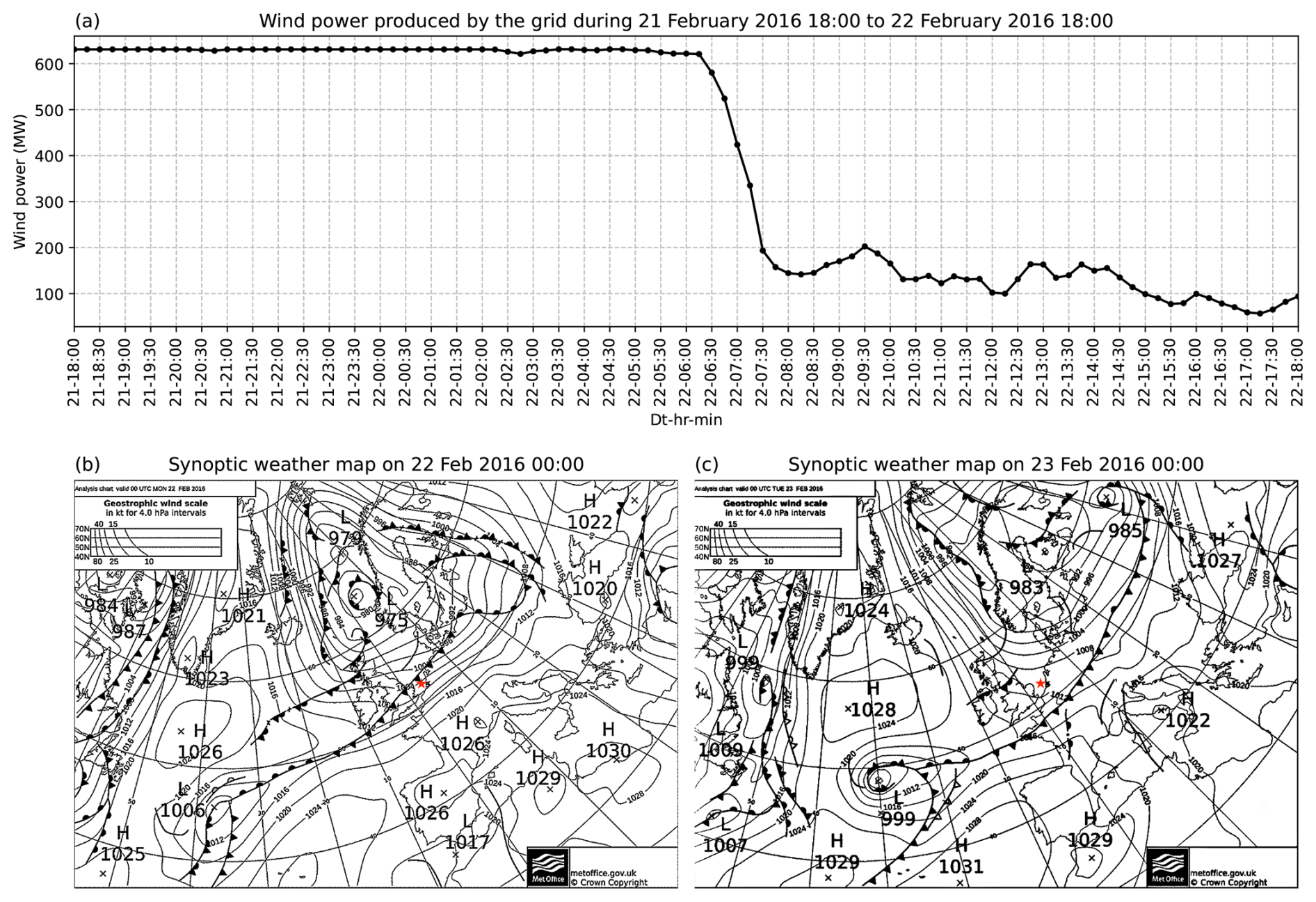
Figure 1 (a) The time series of wind power produced by the Belgian offshore wind farms, from 18:00 UTC on 21 February to 18:00 UTC on 22 February 2016, which depicts the extreme power ramp. The total capacity of the wind farms is 712 MW. Source: https://www.elia.be (last access: 21 July 2025). (b) Synoptic weather maps on 00:00 UTC on 22 February and (c) 23 February 2016, illustrating a cold front (represented by the black line with filled triangles, pointing towards the frontal movement) passing over the Belgium offshore wind farm (illustrated with the red star). Source: https://www.wetterzentrale.de/ (last access: 21 July 2025).

3.1.2 Case 2

Similarly to the above, on 4 March 2016, BOWFC experienced an 88 % drop in its measured wind power within 1 h, beginning from 07:00 UTC, as shown in Fig. 2a. The farm is seen producing power of more than 620 MW for 4 h before experiencing the severe ramp-down event. The synoptic weather charts at 00:00 UTC on 4 (Fig. 2b) and 5 March (Fig. 2c) show that a cold front overpassed the wind farm during this period.

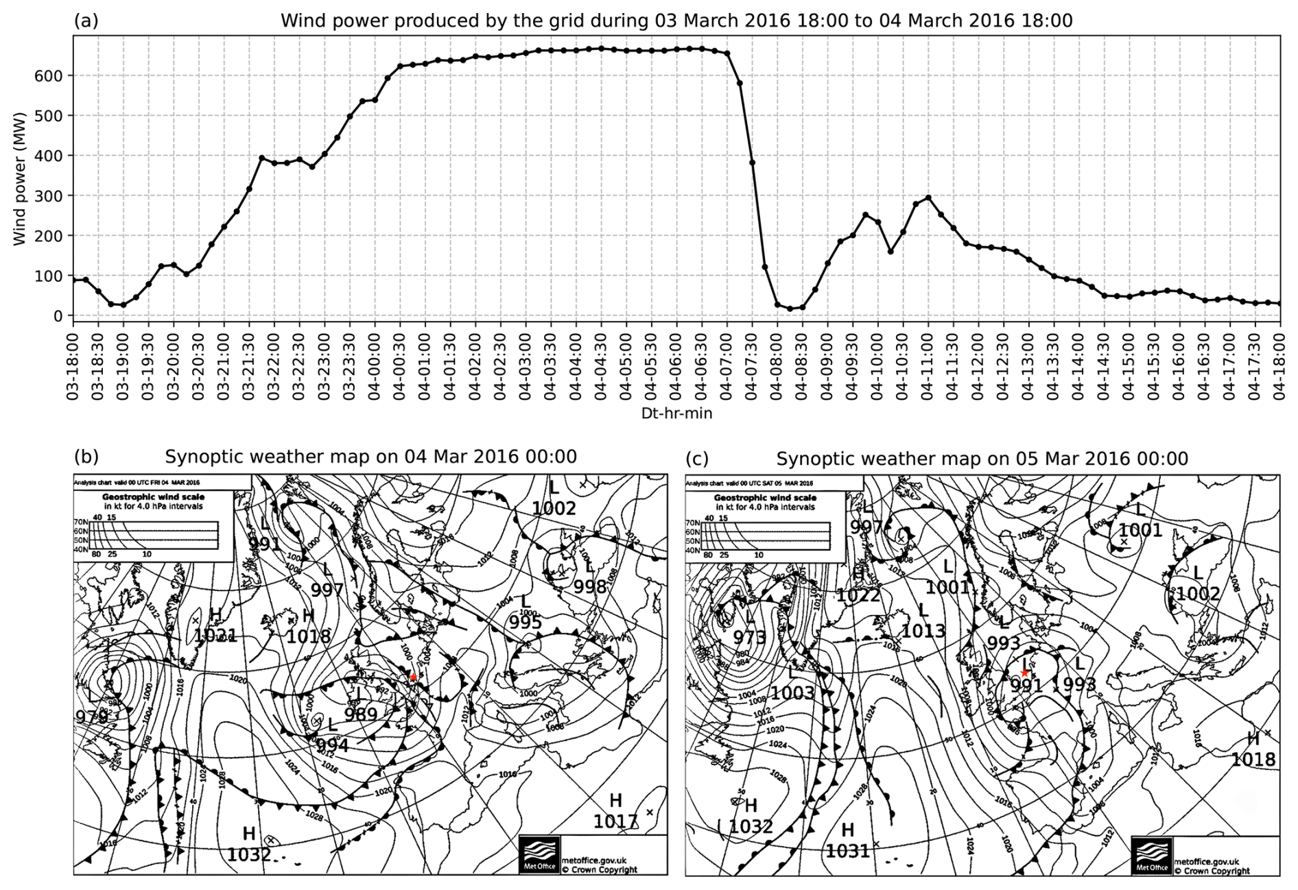
Figure 2 Same as Fig. 1 but for case 2. (a) The time series of wind power produced by the Belgian offshore wind farms, from 18:00 UTC on 3 March to 18:00 UTC on 4 March 2016, which depicts the extreme power ramp. (b) Synoptic weather maps at 00:00 UTC on 4 March 2016 and (c) 00:00 UTC on 5 March 2016, illustrating a cold front passing over the Belgium offshore wind farm (illustrated with the red star).

3.2 Model configuration

In this study, the WRF model (version 4.4) is utilized to simulate the identified cases. For the sensitivity analysis, we chose to vary the initial and boundary conditions, using ERA5 and CERRA datasets to represent hindcast experiments and the Global Forecasting System (GFS) to represent the forecast experiment. Additionally, we varied the domain configuration, planetary boundary layer (PBL) schemes, and activation of wind farm parameterization, in conjunction with the hindcast experiments. In total, five hindcast sensitivity experiments and one forecast experiment were designed, as summarized in Table 1. The innermost domain of all the WRF runs is illustrated in Fig. 3, which is consistently maintained across the runs.

Table 1 Overview of the WRF model simulations.

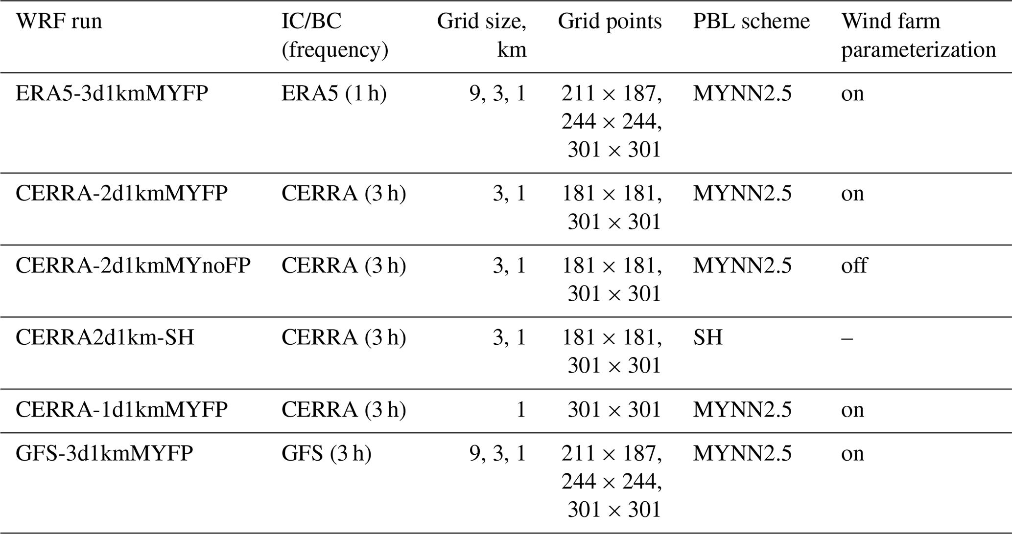
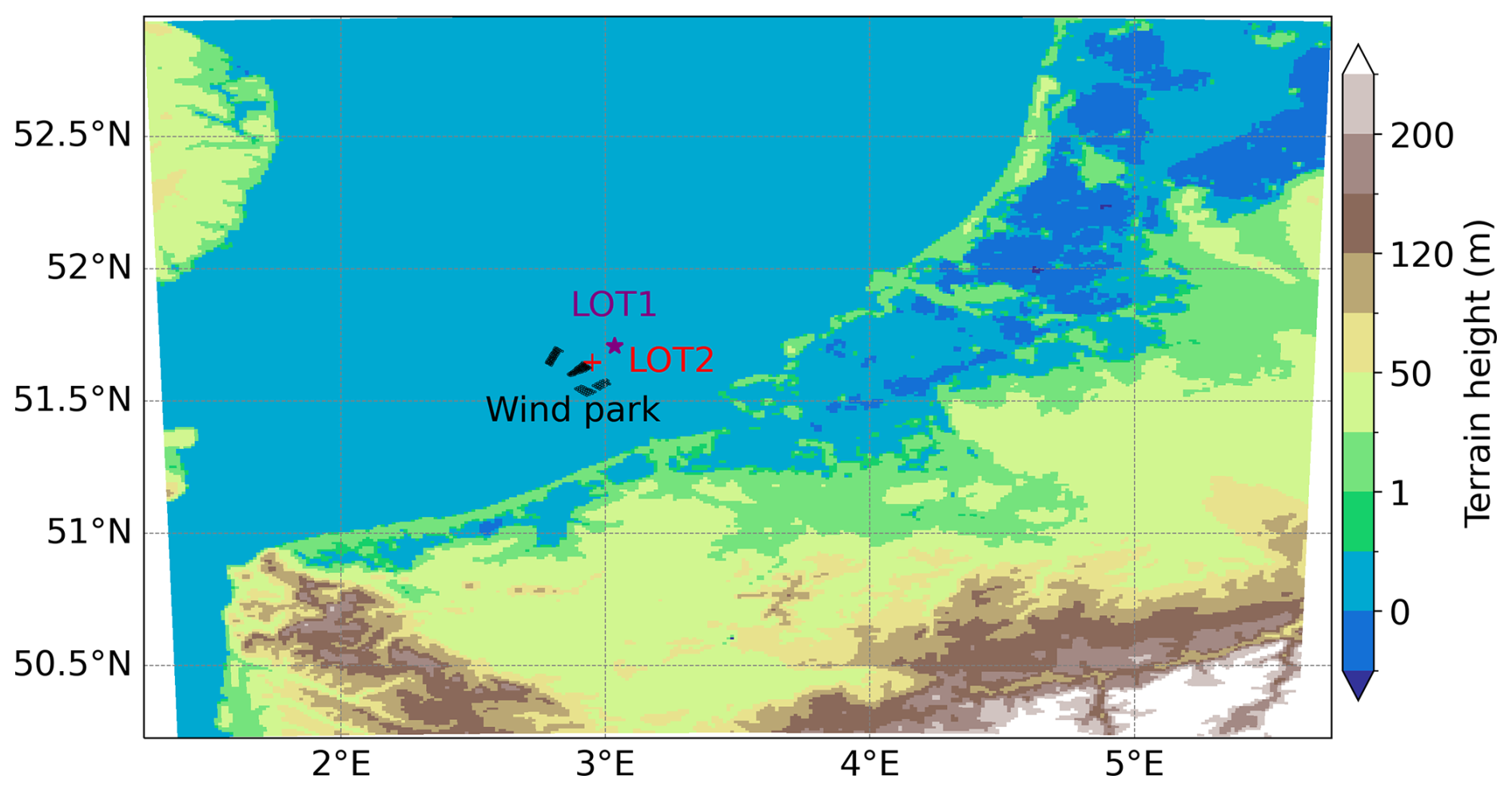
Figure 3 A topographical overview of the WRF model simulation domain, encompassing the interested region, consisting of the Belgium offshore wind farm (illustrated with dark filled circles) and two buoy observational locations – LOT1 (illustrated with the purple star) and LOT2 (illustrated with the red plus). This domain is the innermost domain, which is D03 in ERA5-3d1kmMYFP; D02 in CERRA-2d1kmMYFP, CERRA-2d1kmMYnoFP, and CERRA-2d1kmSH; and D01 in CERRA-1d1kmMYFP simulations.

3.2.1 Initial and boundary conditions

We have explored two options for the initial and boundary conditions (IC/BCs) in the hindcast experiments – ERA5 and CERRA. ERA5 has been released progressively since 2017, and soon after its introduction, it became the preferred reanalysis dataset in the wind power meteorology community. Several studies, like Olauson (2018), Ramon et al. (2019), Gualtieri (2022), and many others, discuss its superior accuracy, lower uncertainty, and higher reliability compared to other global reanalysis datasets. The dataset is available at an hourly resolution and a horizontal grid spacing of about 30 km. In this study, the ERA5-3d1kmMYFP runs utilize the ERA5 reanalysis at an hourly update frequency as forcing data.

CERRA provides a high-resolution pan-European reanalysis with a 5.5 km horizontal resolution and 106 vertical levels, covering Europe, northern Africa, and the southeastern parts of Greenland. The dataset is essentially downscaled from the global ERA5 reanalysis. Unlike the ERA5 data, CERRA provides analysis every 3 h. Despite the advantages of CERRA, the data have never been used as driving data for simulations and have not been incorporated into the WRF model configuration. Thus, we aim to capitalize on the fine-scale resolution of CERRA in simulating the extreme ramps associated with FLLJ events. In doing so, a novel hybrid CERRA- and ERA5-based WRF simulation strategy has been developed in this study.

In order to successfully incorporate new forcing data into the WRF model, a new vtable file needs to be constructed according to the data specifications. After a thorough investigation, it was found that all surface- and upper-level meteorological variables needed for the model simulations exist in the CERRA analysis, except soil moisture and soil temperature. Additionally, the WRF model recognizes the U and V components of winds, so the 10 m wind speed and direction from the CERRA data are transformed into 10 m U and V components. A new vtable corresponding to the CERRA data is created according to the information provided in the downloaded data files. The CERRA analysis data are ungribbed first using the created vtable file, while the soil moisture and soil temperature variables from ERA5 reanalysis are ungribbed later using a different vtable file. After this step, the final metfiles are created, incorporating all the required meteorological variables for the WRF simulations. Except for ERA5-3d1kmMYFP, the remaining WRF runs utilize the CERRA analysis at a 3-hourly update frequency as forcing data.

The sensitivity to driving data in hindcast experiments is assessed through the WRF runs ERA5-3d1kmMYFP and CERRA-2d1kmMYFP. Since ERA5 reanalysis exists at 32 km resolution, we opted for three one-way nested domains for ERA5-3d1kmMYFP runs, consisting of horizontal grid spacings of 9, 3, and 1 km in the domains d01, d02, and d03, respectively. On the other hand, the CERRA analysis exists at 5.5 km resolution; thus we chose two one-way nested domains for CERRA-2d1kmMYFP runs, consisting of horizontal grid spacings of 3 and 1 km in the domains d01 and d02, respectively. We used the pressure level datasets from both ERA5 and CERRA as initial and boundary conditions in our simulations.

The initial and boundary conditions provided by the reanalysis datasets (e.g., ERA5 and CERRA) tend to be very accurate due to extensive data assimilation. However, in the context of real-time forecasting, such high-fidelity boundary conditions are not available; thus operational forecast data from global models (e.g., GFS) can be used. In the forecast experiment GFS-3d1kmMYFP, cases 1 and 2 are forecasted using a similar configuration to ERA5-3d1kmMYFP, except with GFS real-time forecast data provided as initial and boundary conditions (National Centers for Environmental Prediction, National Weather Service, NOAA, U.S. Department of Commerce, 2015). The GFS IC/BCs during the simulation period are available at a 3-hourly resolution and a horizontal grid spacing of about 30 km.

3.2.2 Wind farm parameterization

The wind farm parameterization (WFP) by Fitch et al. (2012) represents the effects of the wind turbines as a drag-induced energy sink and increased turbulence in the vertical levels containing the rotor disk. The Fitch parameterization assumes that a fraction of the total energy flowing through the wind farm is used for power production (based on the turbine power coefficient), and the rest is converted into turbulent kinetic energy (determined by the turbine thrust coefficient). During the study period, BOWFC consisted of three Belgian offshore wind farms: C-Power, Northwind, and Belwind I, populated with five different types of wind turbines. The wind farms are illustrated as dark filled circles in Fig. 3. More details about each wind turbine, including the power curve, thrust curve, and their corresponding sources, can be found in Li et al. (2021).

The Fitch WFP is well known for simulating turbine effects; thus it is expected that activating this scheme would result in better wind speed and power simulations. However, the parameterization is only coupled with the Mellor–Yamada–Nakanishi–Niino 2.5 (MYNN2.5) PBL scheme. To understand the significance of this WFP scheme, we conducted the WRF run CERRA-2d1kmMYnoFP with the WFP turned off, while it was turned on in the remaining runs with the MYNN2.5 PBL scheme. The sensitivity to Fitch WFP is assessed through the WRF runs CERRA-2d1kmMYFP and CERRA-2d1kmMYnoFP.

3.2.3 Planetary boundary layer scheme

Previous studies have emphasized the critical role of PBL schemes in accurately representing wind interactions and turbulence in the lower atmosphere, specifically at the wind turbine hub height (Nunalee and Basu, 2014; Gevorgyan, 2018; Vemuri et al., 2022). Therefore, we chose two different PBL schemes, namely the MYNN2.5 scheme (Mellor and Yamada, 1982; Nakanishi and Niino, 2006, 2009), which has been employed in many wind energy application studies (Jiménez et al., 2015; Jahn et al., 2017; Li et al., 2021), and the Shin Hong (SH) scheme (Shin and Hong, 2015), which is a scale-aware scheme, adopted from the studies of Vemuri et al. (2022). The sensitivity to the PBL scheme is assessed through the WRF runs CERRA-2d1kmMYnoFP (without Fitch parameterization) and CERRA-2d1kmSH (inherently no WFP).

The MYNN2.5 and SH PBL schemes differ fundamentally in their approach to turbulence and mixing. MYNN2.5, as a local scheme, relies solely on resolved variables from adjacent grid points to calculate turbulence. In contrast, the SH scheme is nonlocal, using information from multiple vertical levels to determine mixing. It employs scale-aware adjustments and mixing approaches, such as counter-gradient terms or grid-size dependency, to better capture the interplay between the boundary layer and the free atmosphere.

3.2.4 Domain configuration

The CERRA analysis exists at 5.5 km resolution, which makes it possible to configure the model domain at kilometer resolution without the need for nesting. Thus, to examine the sensitivity to domain configuration, we configured the CERRA-1d1kmMYFP run with a single domain at 1 km resolution. The sensitivity to domain configuration is assessed through the WRF runs CERRA-2d1kmMYFP and CERRA-1d1kmMYFP.

3.3 Simulation setup

In this study, the MYNN surface-layer scheme (Smirnova et al., 2021) is used in combination with the MYNN2.5 PBL scheme, while the revised MM5 surface-layer scheme (Jiménez et al., 2012) is adopted for the experiments with the Shin Hong PBL scheme. For the simulations with the MYNN2.5 PBL scheme, we set bl_mynn_tkebudget = 1 and bl_mynn_tkeadvect = .true. for the bl_mynn settings, while the other settings are unaltered, taking their default settings. The remaining physics schemes, including the WRF single-moment five-class scheme for microphysics (Hong et al., 2004), RRTMG for shortwave and longwave radiation (Iacono et al., 2008), unified NOAH for land surface physics (Tewari et al., 2004), and Kain–Fritsch for cumulus physics (Kain, 2004), are adopted from the studies of Li et al. (2021). The simulations are conducted with a total of 50 vertical levels, spanning approximately 8 m above the surface to around 16 km high, with non-uniform grid spacing. The lowest 1 km of the model atmosphere comprises 18 levels. The choice of 50 vertical levels and the corresponding resolution was adopted from Nunalee and Basu (2014).

Event 1 is simulated from 12:00 UTC on 21 February 2016 to 18:00 UTC on 22 February 2016, while event 2 is simulated from 12:00 UTC on 3 March 2016 to 18:00 UTC on 4 March 2016. The GFS IC/BCs initialized at 12:00 UTC on 21 February 2016 for case 1 and at 12:00 UTC on 3 March 2016 for case 2 are obtained for the forecast experiment. The simulations are run for a total of 30 h, with the initial 6 h considered a spin-up period. Output variables, namely wind speed and direction, are recorded at 5 min intervals. If the WFP is activated, the WRF simulation can directly provide wind power production data. For simulations without WFP, wind power production is calculated based on King et al. (2014), who utilize turbine power curves and wind speed at hub height.

3.4 Ramp statistics

In the context of power ramp analysis, we adopt a methodology akin to that of Drew et al. (2018). A percentage drop in wind power with respect to the rated power is used to capture the intensity and timing of the ramp event, which is computed as,

$$\begin{array}{}\text{(1)}& \mathit{\%}\mathrm{\Delta }P={\displaystyle \frac{P_{t+\mathrm{\Delta }t}-P_t}{P^{*}}}\times \mathrm{100}.\end{array}$$

Here, P^* is the rated grid power and P_t is the simulated power at time instance t. The timescales Δt are taken at 15 min, 30 min, and 1 h to quantify the ramp rates.

4 Results

4.1 Wind power time-series comparison

The time-series data presented in Fig. 4 compare wind power outputs from five WRF simulations to the actual production of the wind farm for two cases. In case 1 (Fig. 4a), the wind farm experienced a significant decrease in power output starting at 06:30 UTC, while in case 2 (Fig. 4b), this decline commenced at 07:00 UTC, as detailed in the case descriptions.

During the pre-ramp period (from the starting point to the ramp occurrence), the wind farm produced a consistent maximum power output, which is attributed to the peak winds associated with the FLLJ. Interestingly, the power output is slightly below the rated capacity of 712 MW. This shortfall is likely due to some turbines being curtailed to prevent damage during high wind speeds or not being in operation. On the other hand, all the WRF model simulations produced power output at the rated capacity, implying that the FLLJ was simulated well. All the simulations produced substantial power drops during the ramp period in both cases, albeit with timing and amplitude discrepancies.

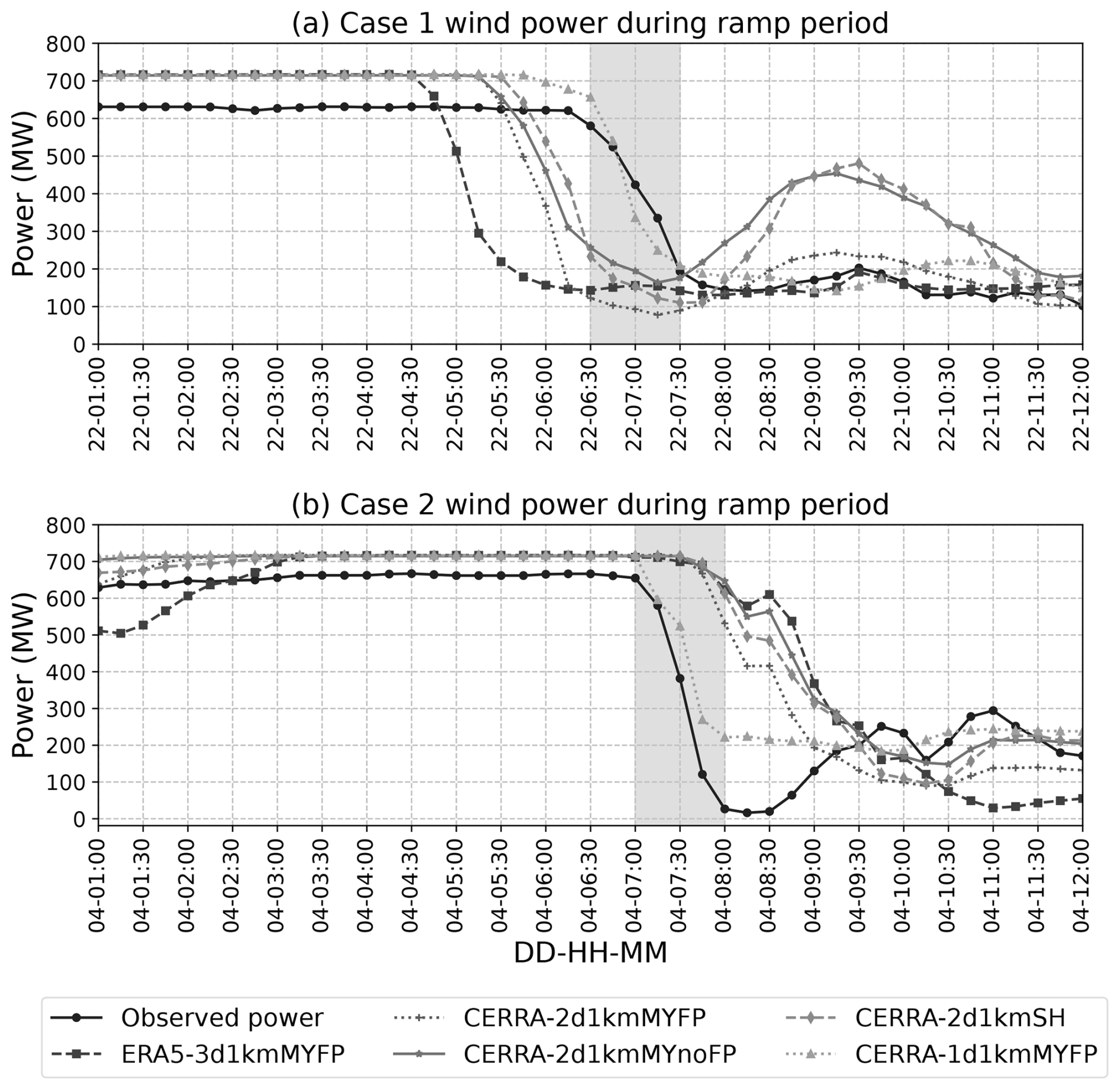
Figure 4 A comparison of wind power time series from the five WRF model simulations and the Belgium offshore wind farm production. (a) From 01:00 to 12:00 UTC on 21 February 2016 for case 1. (b) From 01:00 to 12:00 UTC on 4 March 2016 for case 2. The ramp period (1 h) is shaded in gray.

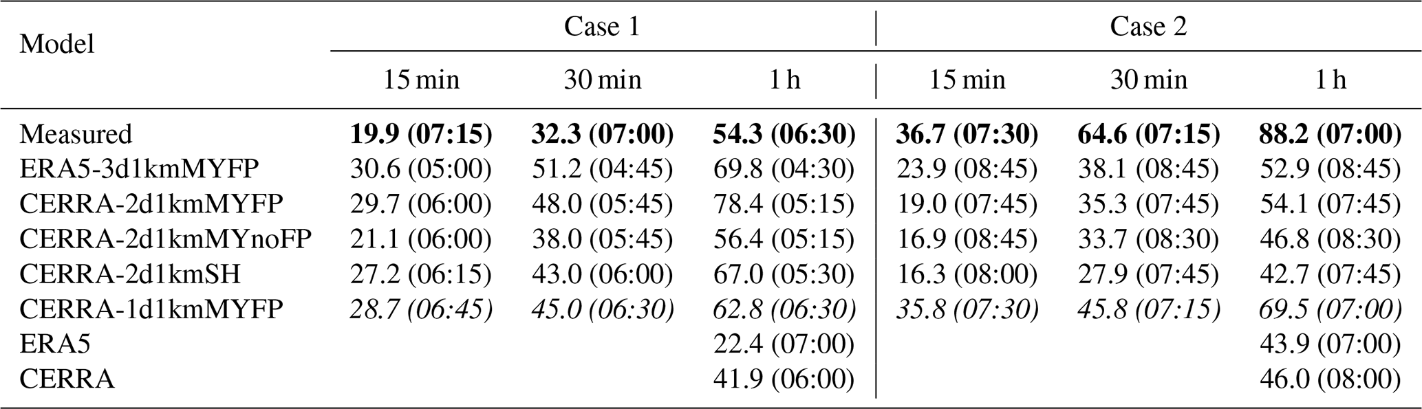
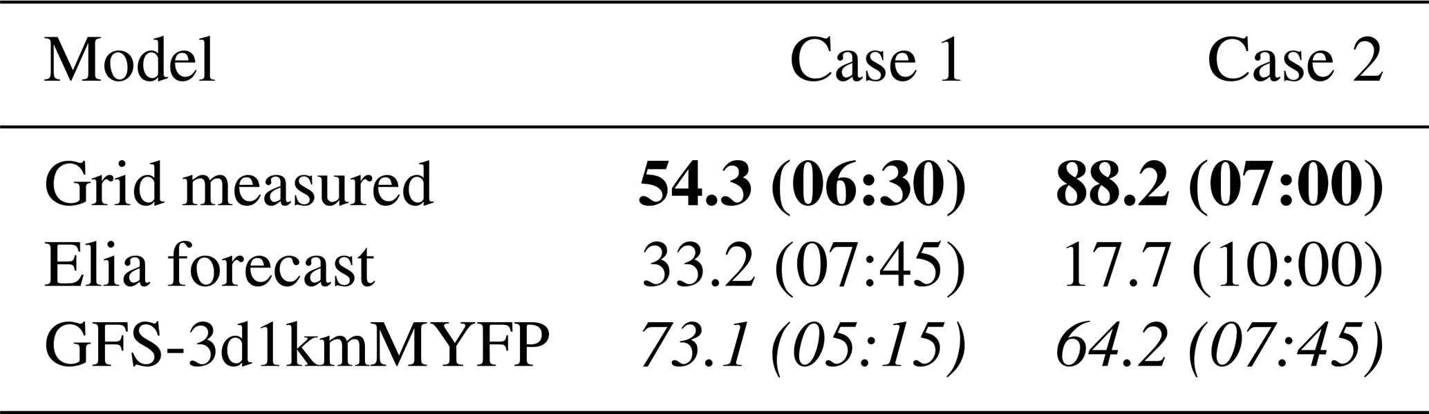
The ramp statistics are computed using Eq. (1) and are listed in Table 2 for both cases. In case 1, the wind farm's power output decreased by 19.9 % within 15 min from 07:15 UTC, by 32.3 % within 30 min from 07:00 UTC, and by 54.3 % within 1 h from 06:30 UTC. However, the WRF simulations tend to overestimate the intensity of these power drops. Despite overestimating the intensity of the ramp event, the CERRA-1d1kmMYFP simulation matched the ramp timing well. This discrepancy is attributed to the rated power production prior to the onset of the power ramp.

In case 2, the wind farm experienced power drops of 36.7 %, 64.6 %, and 88.2 % within 15, 30, and 60 min from 07:30, 07:15, and 07:00 UTC, respectively. In contrast to case 1, all the WRF simulations underestimated the ramp intensities across the timescales. Among all, only the CERRA-1d1kmMYFP simulation closely reproduced both the timing and the intensity of the power drop, with a 69.5 % decrease within 1 h, matching the observed timing of 07:00 UTC.

To highlight the necessity of dynamical downscaling, wind power output is computed using wind speed from ERA5 model levels (https://cds.climate.copernicus.eu/datasets/reanalysis-era5-complete?tab=d_download, last access: 21 July 2025) and CERRA height levels (https://cds.climate.copernicus.eu/datasets/reanalysis-cerra-height-levels?tab=download, last access: 21 July 2025). The corresponding ramp statistics are presented in Table 2. The results indicate that ramp timings derived from both datasets closely align with those from WRF simulations and observations. However, the ramp intensity is significantly underestimated by ERA5, whereas CERRA exhibits a moderate underestimation.

Table 2 Overview of the ramp statistics in wind power in terms of intensity (%) and timing (in parentheses) at three timescales: 15, 30, and 60 min, obtained from the wind power produced by the Belgium offshore wind farm and the five WRF simulations, during case 1 and case 2. The ramp statistics from measured wind power are presented in bold text, while the best-performing simulation is italicized. The ramp statistics at a 60 min timescale from ERA5 and CERRA are also presented. All times are in UTC.

Comparing the ERA5-3d1kmMYFP and CERRA-2d1kmMYFP simulations, the ERA5 IC/BCs tend to produce ramps at significantly different times, either earlier or later, although their amplitudes are similar to those of the CERRA IC/BCs.

In the comparison between CERRA-2d1kmMYFP and CERRA-2d1kmMYnoFP, the Fitch WFP consistently simulates lower power output than the no-FP run. This discrepancy is attributed to the interaction of wind turbines with the flow and the generation of wind wakes. To investigate further, 100 m level wind speed spatial plots from both simulations were examined at various time points for cases 1 and 2, as shown in Figs. F1 to F4 in the Appendix. The Fitch WFP clearly produced wakes, indicated by a wind speed deficit of 2 m s⁻¹ along the wind direction. These wakes extend much farther during FLLJ periods. Due to wake generation, the wind speed simulated by the CERRA-2d1kmMYFP run is slower than that of its counterpart. Aside from the vicinity of the wind farm, wind speeds in both runs are almost identical elsewhere.

When comparing CERRA-2d1kmMYnoFP and CERRA-2d1kmSH, the wind power time series are largely similar across cases. The scale-aware SH scheme captures ramp timing better, while the MYNN2.5 scheme captures ramp intensity marginally better. However, these differences are minimal.

In the comparison between CERRA-2d1kmMYFP and CERRA-1d1kmMYFP, the domain configuration, such as nesting two domains versus a single domain, significantly influences power output. The single-domain configuration in both cases reproduced the power time series more accurately, matching the observed data, unlike its counterpart. Additionally, ramp timing and intensities are captured better by the single-domain setup.

Apart from the aforementioned configurations, we also examined the influence of the number of vertical levels and the choice of spin-up time on simulation accuracy, as discussed in Appendixes B and C. From the analysis, we observed that increasing the number of vertical levels from 50 to 100 moderately deteriorated simulation accuracy. This indicates that higher vertical resolution, while theoretically promising, can introduce complexities that negatively impact model performance under specific conditions. On the other hand, increasing the spin-up time from 6 to 12 h did not result in any significant alterations, suggesting that a 6 h spin-up period is sufficient for the development of the meteorological features of the weather phenomenon under study.

Overall, there is clear evidence of sensitivity in ramp timing and amplitude with respect to the modeling parameters, with domain configuration and the WFP being the most influential factors.

4.2 Wind speed and direction time-series comparison

The wind speed time series at different vertical levels from lidar observations at the LOT2 location for cases 1 and 2 are illustrated in Fig. 5a–a*. In both cases, a significant drop in wind speed is clearly evident. What distinguishes the two cases is that during the pre-ramp period, there are significant wind speed shears within the 30–200 m layer in case 1, whereas they are only slightly noticeable in case 2. Furthermore, the wind speed drop around 06:00 UTC in case 1 is drastic, whereas in case 2, it occurs more gradually from 06:00 to 07:00 UTC. Nonetheless, in both cases, the wind speed drops at all vertical levels, reaching as low as 6 m s⁻¹ from as high as 20 m s⁻¹ in case 1 and 5 m s⁻¹ from 17 m s⁻¹ in case 2. Comparing the wind speed time series with the wind power data, it becomes evident that the ramp timing is 1 h ahead in wind speed. This can be explained by the movement of the front and spatial distribution of wind farms, which cannot experience the ramp all at once, whereas lidar observations are measured at a single point.

Similarly, the wind direction time series from lidar observations at the LOT2 location for cases 1 and 2 are illustrated in Fig. 5a–a*. Significant wind directional shifts, approximately 100° in case 1 and 130° in case 2, are evident in both cases. These shifts align with the wind speed ramp timings, indicating that the wind speed ramp was accompanied by sharp wind directional changes. Unlike the wind speed shears, there are no visible wind veers between the 30–200 m layer, except for occasional fluctuations.

The WRF-simulated wind speed from the five runs is illustrated in Fig. 5b–f and b*–f*, while direction time series from five runs are illustrated in Fig. 6b–f and b*–f*. Comparing ERA5-3d1kmMYFP and CERRA-2d1kmMYFP, the simulations forced with CERRA reanalysis were able to reproduce the drastic wind speed drop and wind directional shift in both cases, albeit with considerable timing errors, compared to the observations. Similarly, the simulations forced with ERA5 also reproduced a strong wind speed drop and directional shift in case 1. However, in case 2, the ramp is more gradual, spanning several hours, with a strong directional shift visible 3 h later than observed.

The reason for these discrepancies is examined through 100 m wind speed time series obtained from the original forcing datasets, as shown in Fig. D1. ERA5 shows a wind speed drop of 3 m s⁻¹ in case 1 and 4 m s⁻¹ in case 2 within 1 h, whereas CERRA shows a drop of 9 m s⁻¹ in case 1 and 4.5 m s⁻¹ in case 2. From these observations, it is deduced that the coarser representation of the atmosphere in the ERA5 forcing data led to poor dynamical downscaling through the WRF model. In contrast, the better representation in CERRA resulted in more intense wind speed ramp simulations.

Comparing CERRA-2d1kmMYFP and CERRA-2d1kmMYnoFP, the winds simulated by the Fitch WFP are 0.5–1 m s⁻¹ lower than those of the counterpart. This is due to the generation of wakes by the WFP, which reduces wind speed within the vicinity of the wind farm, as discussed earlier. Apart from the reduced wind speed, the wind speed and directional time series are identical to one another, with little to no variations.

Comparing CERRA-2d1kmMYnoFP and CERRA-2d1kmSH, the wind speed and directional time series show some degree of similarity during the pre-ramp and ramp periods. However, the winds simulated by the scale-aware SH scheme across the cases are consistently lower than those of the counterpart and also closely align with the observations. In addition, the wind speed ramp in case 2 is abrupt from the MYNN2.5 scheme, while the SH scheme simulated an initial sharp ramp followed by a gradual reduction in winds to 5 m s⁻¹. These discrepancies suggest that the PBL scheme has some degree of influence on the wind speed and direction simulation.

Comparing CERRA-2d1kmMYFP and CERRA-1d1kmMYFP, the wind speed and direction produced by the single-domain configuration are consistently lower than those from the nested-domain configuration. In fact, the wind speed time series during the pre-ramp period from the single-domain configuration are very close to the observed ones, with an intermittent wind speed drop in case 1 and a gradual rise in wind speed during case 2. The CERRA-1d1kmMYFP simulation is particularly interesting, as it perfectly captured the ramp timing in both cases. However, in case 1, it reproduced a secondary gradual down-ramp, which is not seen in the observations or produced by the nested-domain configuration.

Since downscaling is largely governed by the forcing data, the nested-domain configuration simulations will modify the initial and boundary conditions (IC/BCs) considerably due to telescopic refining, while the single-domain simulations remain closer to the original IC/BCs. Thus, the better accuracy observed in the single-domain configuration simulation is attributed to the more accurately resolved atmospheric features present in the CERRA IC/BCs.

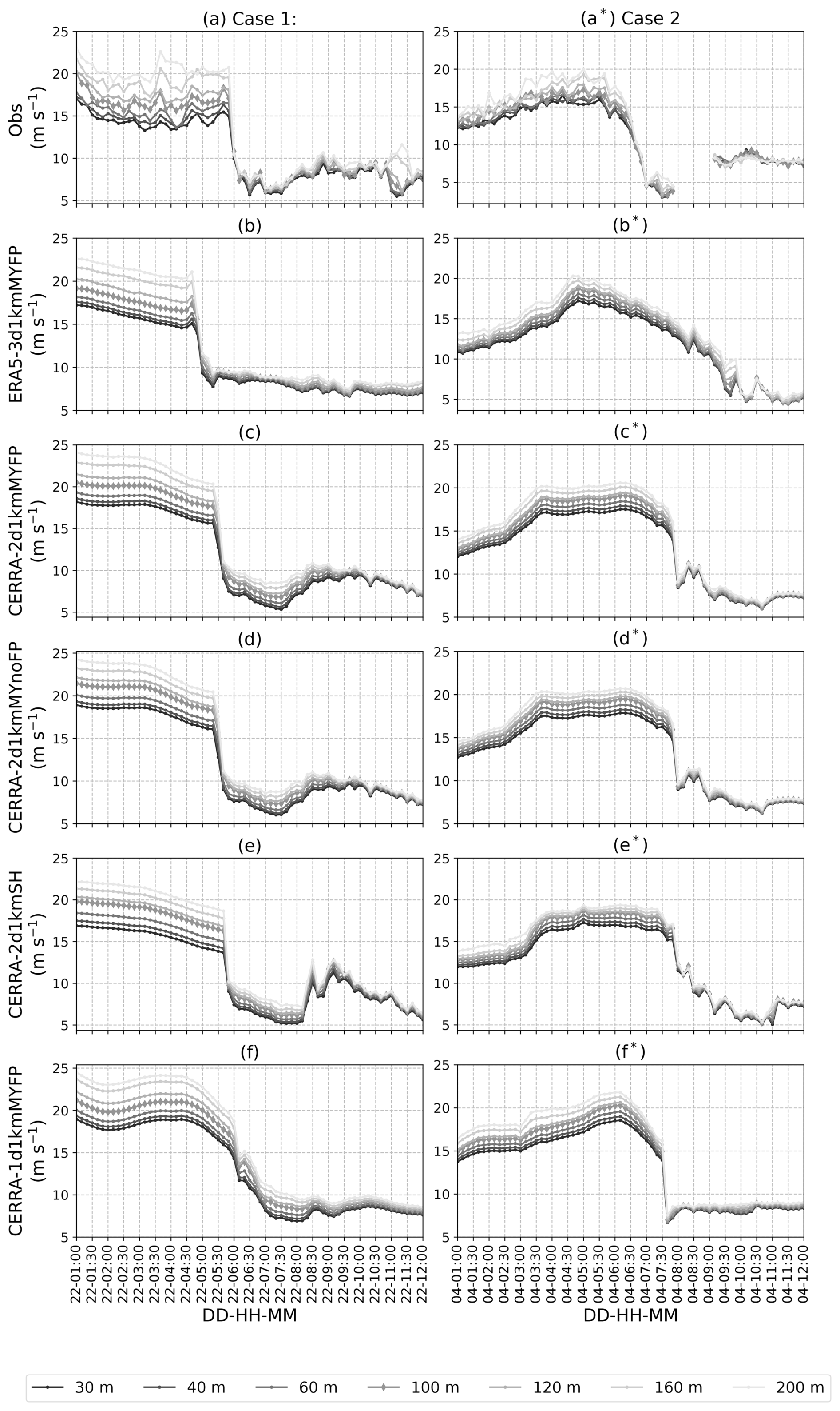
Figure 5 A comparison of wind speed time series at seven vertical levels from lidar observations at LOT2 (a–a*) and the five WRF model simulations (b–f and b*–f*) (b–f) From 01:00 to 12:00 UTC on 21 February 2016 for case 1. (b*–f*) From 01:00 to 12:00 UTC on 4 March 2016 for case 2.

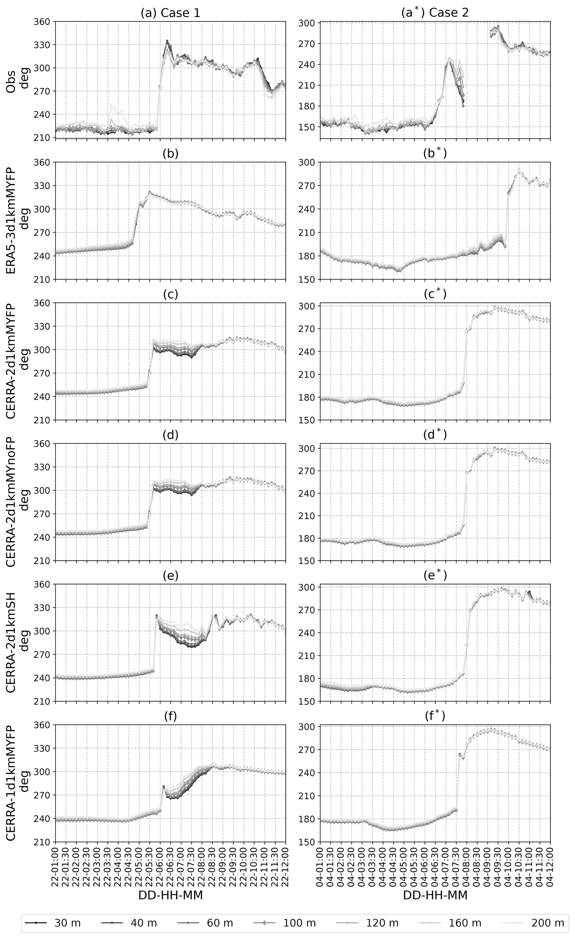
Figure 6 A comparison of wind direction time series at seven vertical levels from lidar observations at LOT2 (a–a*) and the five WRF model simulations (b–f and b*–f*). (b–f) From 01:00 to 12:00 UTC on 21 February 2016 for case 1. (b*–f*) From 01:00 to 12:00 UTC on 4 March 2016 for case 2.

4.3 Wind profiles

To identify the FLLJ and its characteristics in terms of core strength and height, we need wind speed profiles spanning the entire boundary layer. Unfortunately, lidar observations only measure wind speed up to 200 m, which is inadequate for characterizing FLLJs. As an alternative, we utilized the WRF-simulated wind profiles from five runs for the analysis. Knowing that the jet occurs during the pre-ramp period, we extracted the hourly averaged wind speed profiles during different time instances at the LOT2 location, illustrated in Fig. 7 for both cases. Apart from the wind speed profiles, the time–height cross-sections of wind speed at the LOT2 location are also illustrated in Fig. E1.

Although there is no universally accepted definition of an LLJ, in this study, we used the definition from Hallgren et al. (2023): an increase in horizontal wind speed of at least 1 m s⁻¹ and 10 % of the core speed below the jet core (jet nose) and, simultaneously, a decrease of 1 m s⁻¹ and 10 % above the core. The LLJ core height is marked with a solid black line in Fig. E1.

Comparing ERA5-3d1kmMYFP and CERRA-2d1kmMYFP, in case 1, the ERA5 IC/BCs produced diffused wind profiles at all times, with no defined jet nose identified. On the other hand, the CERRA IC/BCs produced a strong FLLJ core at 400 m altitude. In case 2, both IC/BCs produced a defined jet nose, with the CERRA-forced profiles being more diffuse than the ERA5-forced profiles. This suggests that the vertical profiles from the WRF runs are greatly influenced by the forcing data.

To clarify the source of this discrepancy, we investigated the wind speed profiles from the forcing data (metfiles of ERA5 and CERRA simulations' parent domain), as shown in Fig. D2, at 05:00 UTC for case 1 and 06:00 UTC for case 2. Interestingly, the ERA5 forcing data in case 1 resemble an LLJ profile, with a core height at 700 m. However, the ERA5-3d1kmMYFP run failed to reproduce this LLJ profile. Conversely, the CERRA forcing data in case 2 do not resemble an LLJ profile, but the CERRA-2d1kmMYFP run was able to produce an LLJ profile.

Comparing CERRA-2d1kmMYFP and CERRA-2d1kmMYnoFP, the WFP does not seem to have any significant influence on the vertical wind speed profiles, except for the occasional lower jet core height, which can be attributed to the reduced wind speed. Comparing CERRA-2d1kmMYnoFP and CERRA-2d1kmSH, the scale-aware SH scheme results in a stronger FLLJ core at a higher altitude compared to the MYNN2.5 scheme across the cases. Additionally, the FLLJ nose is more defined and pronounced in the scale-aware PBL scheme, suggesting a more accurate representation of the jet characteristics.

Comparing CERRA-2d1kmMYFP and CERRA-1d1kmMYFP, the single-domain configuration notably produced double peaks in case 1, which seem to stem from the forcing data (as observed in the CERRA profiles from Fig. D2), indicating that the downscaling is largely governed by the forcing data here. In both cases, the single-domain configuration produced jet cores at higher altitudes with higher magnitudes than the double nested-domain configuration.

Overall, all simulations were able to produce some degree of the jet core but with varying heights and strengths. Interestingly, the wind profiles are different across the cases, signifying the diversity in the characteristics of the two case studies. Since the profiles are derived from simulations, it is difficult to determine which one is the most accurate. However, it is clear that an FLLJ exists in both cases, with a wind speed maximum (core strength) of 25 m s⁻¹. A clear jet core is located around 700 m in case 2, but there is ambiguity in case 1, where the jet core could be around 400 or 800 m. The differences in the vertical wind speed profiles across the simulations suggest that while FLLJs are a common feature, their precise characteristics can vary significantly depending on the model configuration and resolution.

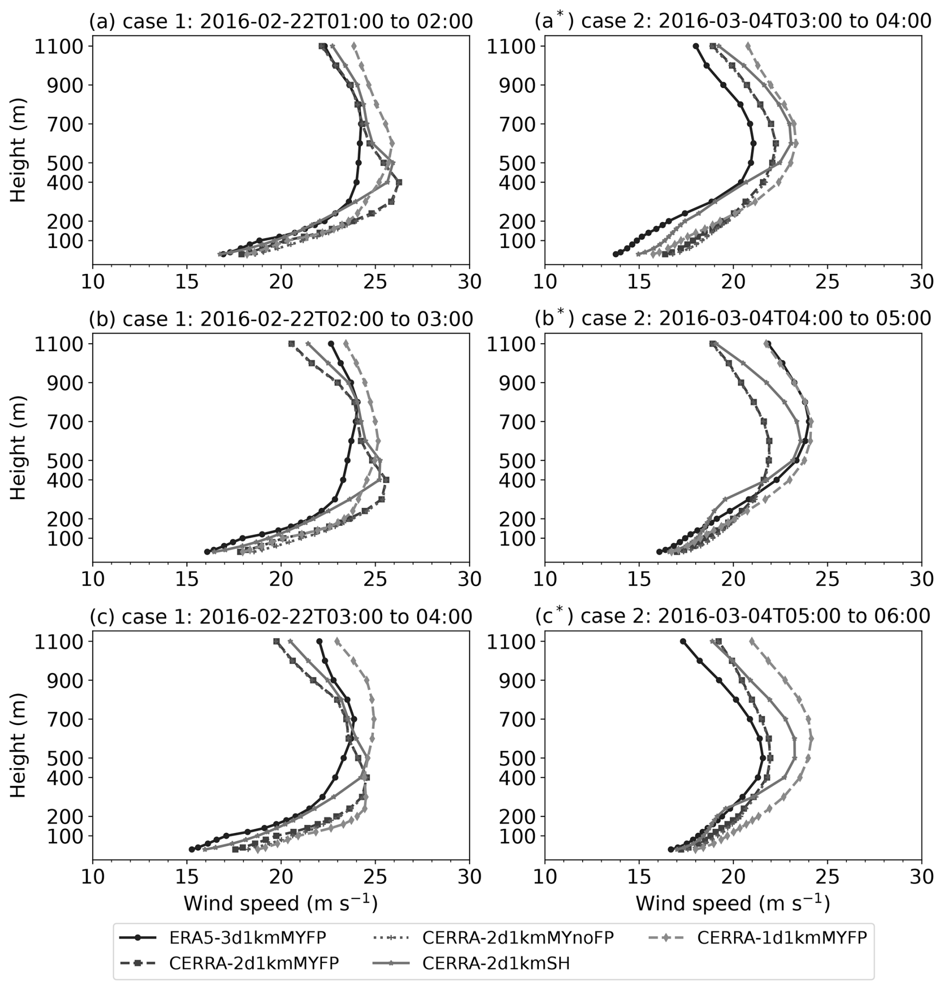
Figure 7 Evolution of wind speed profiles from the five WRF simulations, for case 1 (a–c) and case 2 (a*–c*), at LOT2. The profiles are averaged over hourly intervals from 01:00 to 04:00 (a–c) for case 1 and from 03:00 to 06:00 (a*–c*) for case 2.

4.4 Synoptic characteristics of FLLJ and the associated ramp

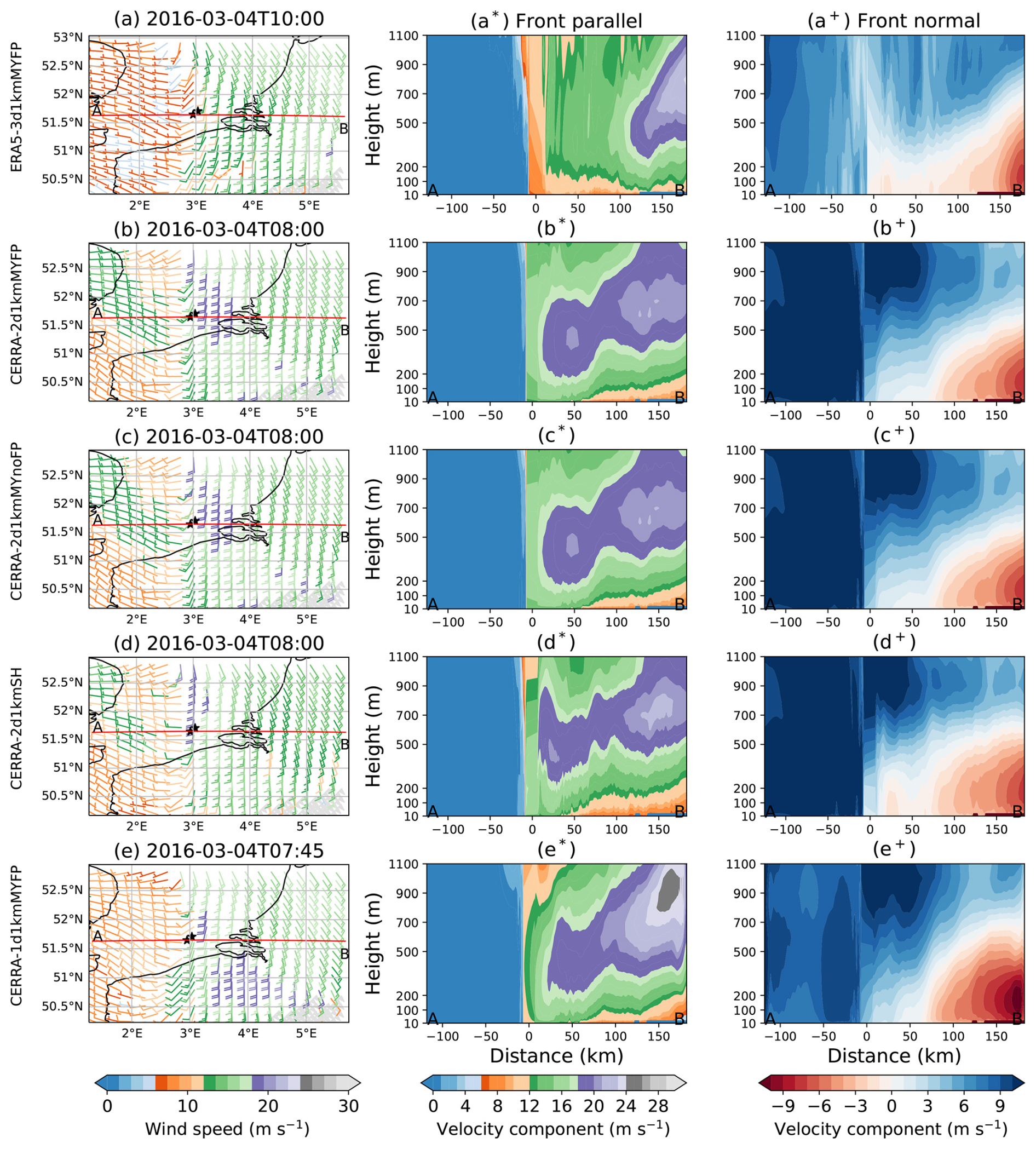
To examine the modeling capability of the WRF model in simulating FLLJs and understanding their synoptic characteristics, we conducted surface and cross-sectional analyses of wind speed. The analysis was performed at the wind speed ramp time instance over the observational site LOT2. From the wind speed time series shown in Fig. 5, it is evident that the WRF runs produced wind speed ramps at different time instances. Thus, to eliminate any influence of a temporal shift on the FLLJ synoptic characteristics, we chose wind speed from each WRF run at the corresponding ramp instance, instead of the lidar-observed ramp instance.

Accordingly, 200 m level wind barbs from the five WRF runs are presented in Fig. 8a–e for case 1 and Fig. 9a–e for case 2. From all the runs, the wind barbs reveal two distinct systematic wind patterns separated by sharp shifts in wind direction. This separation represents the boundary between warm and cold air masses, referred to as the surface cold front (SCF) by Browning and Pardoe (1973). From the WRF runs, the SCF is nearly parallel to the Belgium coast in case 1, while aligning with the 3° longitude in case 2 (except for ERA5-3d1kmMYFP, in which the SCF seems to be curved).

Winds ahead of the frontal boundary, almost parallel to the SCF, are much stronger than the winds trailing the SCF. From the studies of Browning and Pardoe (1973), such strong winds ahead of and parallel to the SCF are indicative of an FLLJ. Conversely, the winds trailing the front, expected to be normal to the SCF, display a slight inclination towards the front in case 1, while remaining perfectly normal in case 2.

Differences in wind speed magnitudes across the WRF runs highlight the influence of modeling parameters. However, the orientation and extent of the FLLJ are consistent across runs, except for ERA5-3d1kmMYFP in case 2. Wind speeds from ERA5-forced runs are generally lower than those from CERRA-forced runs. The WFP has minimal impact on wind speed magnitude. When comparing CERRA-2d1kmMYnoFP with CERRA-2d1kmSH, the scale-aware SH scheme results in lower FLLJ wind speeds than the MYNN2.5 scheme. Additionally, in comparing CERRA-2d1kmMYFP with CERRA-1d1kmMYFP, the single-domain configuration produces consistently lower wind speeds than the nested-domain configuration. Furthermore, the SCF is more distinct in the nested-domain configuration compared to the single-domain configuration.

To gain further insights, a transect line AB (shown in red) was drawn perpendicular to the frontal surface, equivalent to dissecting the frontal cross-section, which serves as a reference for wind speed cross-sectional analysis. The transect-normal velocity component is equivalent to the front-parallel velocity component, shown in Fig. 8a*–e* for case 1 and Fig. 9a*–e* for case 2. The abscissa measures distances (km) along the transect line AB to/from the LOT2 location.

In both cases, regardless of the modeling parameters chosen, a clear and significant wind speed gradient is visible at the LOT2 location (0 km), indicating the presence of the SCF. Ahead of the SCF, from a distance of 10 km, there is a layer of wind speed maxima (jet core) in the vertical direction, indicative of an FLLJ. The choice of IC/BCs, PBL, and domain configuration appears to influence the FLLJ core strength and height.

In case 1, the ERA5 IC/BCs produced a weak core between 300–500 m altitude, while in case 2, no distinct core was formed. In contrast, the CERRA IC/BCs generated a clear jet core in both cases. For case 1, the core height is 400–500 m within 50 km of the SCF, with a core strength of 22–23 m s⁻¹. Beyond this range, orographic interactions cause the jet core to rise, reaching 25 m s⁻¹ at about 100 km distance. In case 2, the core is at 400–600 m with a strength of 21 m s⁻¹ and similarly rises to higher altitudes, reaching 22 m s⁻¹ at approximately 150 km due to orographic interactions.

Comparing CERRA-2d1kmMYnoFP and CERRA-2d1kmSH, the scale-aware SH scheme simulated a higher FLLJ core height in both cases. The core strength is lower in case 1 and higher in case 2 compared to that of MYNN2.5 scheme simulations. Additionally, wind speeds below 200 m are consistently lower in the SH scheme.

For CERRA-2d1kmMYFP versus CERRA-1d1kmMYFP, the single-domain configuration resulted in a higher core height and higher wind speeds below 200 m, producing a more diffused jet nose profile across both cases.

From the cross-sectional analysis, it is clear that the front-parallel component mainly contributes to the occurrence of FLLJs, which is in line with the findings of Browning and Pardoe (1973). On the other hand, the front-parallel winds behind the frontal boundary maintain a magnitude of 8–12 m s⁻¹ in case 1, contributing to the observed directional inclination seen in the wind barbs, whereas a magnitude of 0 m s⁻¹ is seen in case 2, as is evident from the wind barbs.

The transect-parallel velocity component is equivalent to the front-normal velocity component, shown in Fig. 8a⁺–e⁺ for case 1 and Fig. 9a⁺–e⁺ for case 2. Interestingly, velocities ahead of and behind the frontal surface are in the opposite direction and are exactly wedged by the frontal boundary. The findings of Browning and Harrold (1970) confirm that the parallel component behind the front aligns with the frontal surface's movement, while the component ahead of the front directs towards the frontal surface (which actually ascends to the upper levels, not displayed in these figures), a behavior aptly captured by all the simulations.

In both cases, the front-normal velocity ahead of the boundary is much stronger than the velocity behind the boundary. This has two diverse effects: one, winds ahead of the boundary contribute to strengthening FLLJ intensity, and two, winds behind the boundary result in a drastic wind speed drop, ultimately leading to a severe ramp event.

To illustrate the significance of front-parallel and front-normal circulations on wind power production, consider any event. An approaching cold front brings an FLLJ along with it, spanning hundreds of kilometers ahead of the frontal surface and resulting in maximized wind power production for several hours. Within the vicinity of the frontal surface, the front-normal component also contributes to further intensifying the FLLJ. Once the front overpasses a wind farm, wind speed drops from an intense FLLJ magnitude to the magnitude of winds trailing the front, resulting in an intense ramp event.

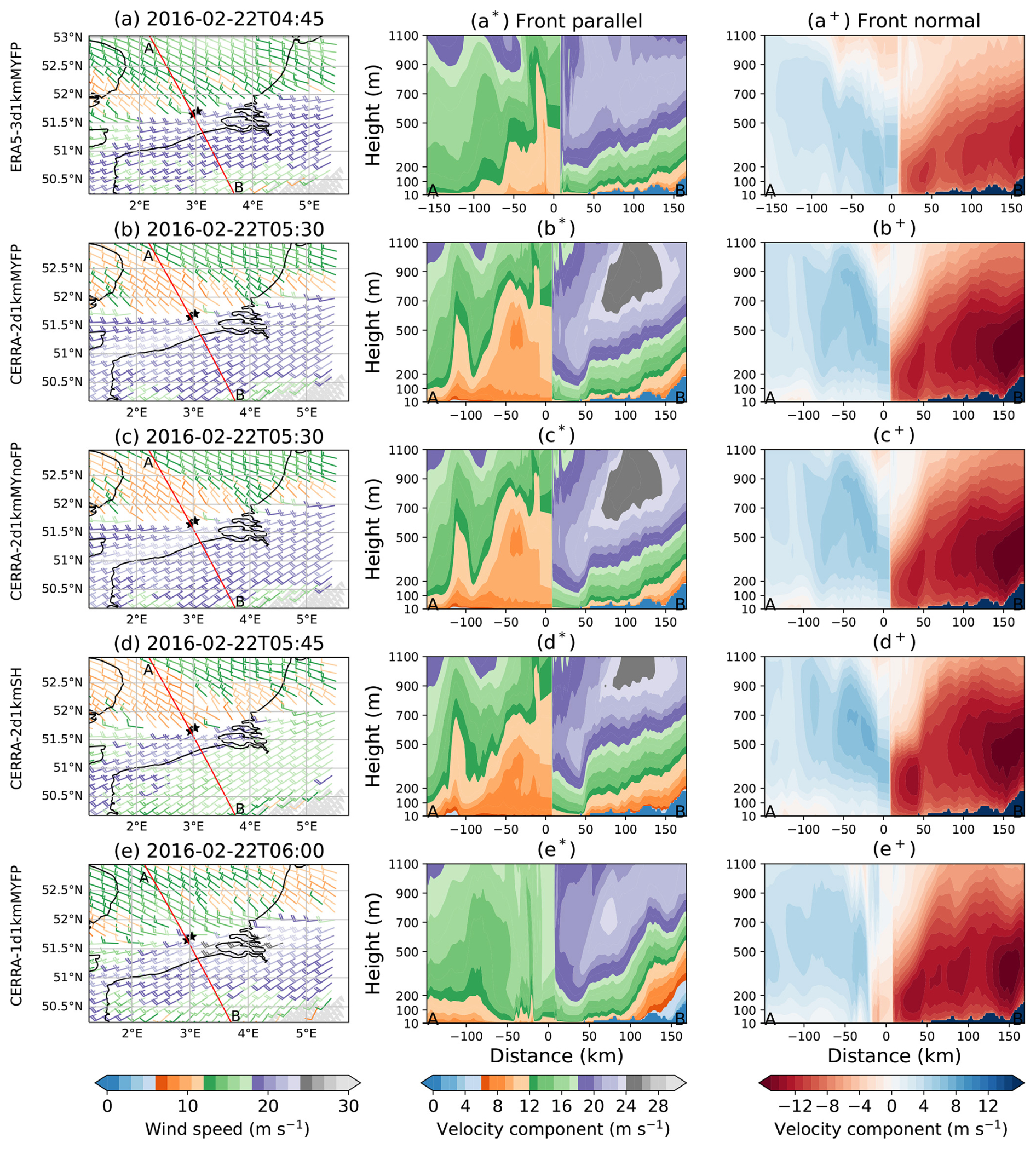
Figure 8 Illustration of horizontal wind speed from the five WRF runs: ERA5-3d1kmMYFP (a–a⁺), CERRA-2d1kmMYFP (b–b⁺), CERRA-2d1kmMYnoFP (c–c⁺), CERRA-2d1kmSH (d–d⁺), and CERRA-1d1kmMYFP (e–e⁺), for case 1, during ramp time instances of the corresponding WRF run. (a–e) Spatial distribution of wind barbs at 200 m level. The ramp instances of the corresponding WRF run are listed as the center title. The transect line AB in red is drawn perpendicular to the frontal surface, while the buoy locations LOT1 and LOT2 are illustrated with black stars. (a*–e*) The velocity component is normal to the transect line AB, which gives an idea of the front-parallel wind speed. (a⁺–e⁺) The velocity component is parallel to the transect line AB, which gives an idea of the front's normal wind speed. The abscissa in the middle and bottom panels is the distance (km) along the transect line AB to/from the LOT2 location, whereas the ordinate is vertical level (m).

Figure 9 Same as Fig. 8 but for case 2 at the ramp instances of the corresponding simulation.

4.5 Real-time forecasting

In this section, we investigate whether extreme ramp events associated with FLLJs could have been predicted in a real-time forecast scenario, through the GFS-3d1kmMYFP run. The model-forecasted wind power is compared with the grid-measured and Elia day-ahead forecast power for cases 1 and 2, as shown in Fig. 10. We note that the WRF model was able to forecast the extreme ramp event in both cases, though with some degree of timing mismatch. In contrast, the Elia forecast shows a gradual ramp-down event in case 1, while no ramp was observed in case 2. Additionally, the model accurately forecasted the pre-ramp wind power maxima, implying that the FLLJs are forecasted well in both cases.

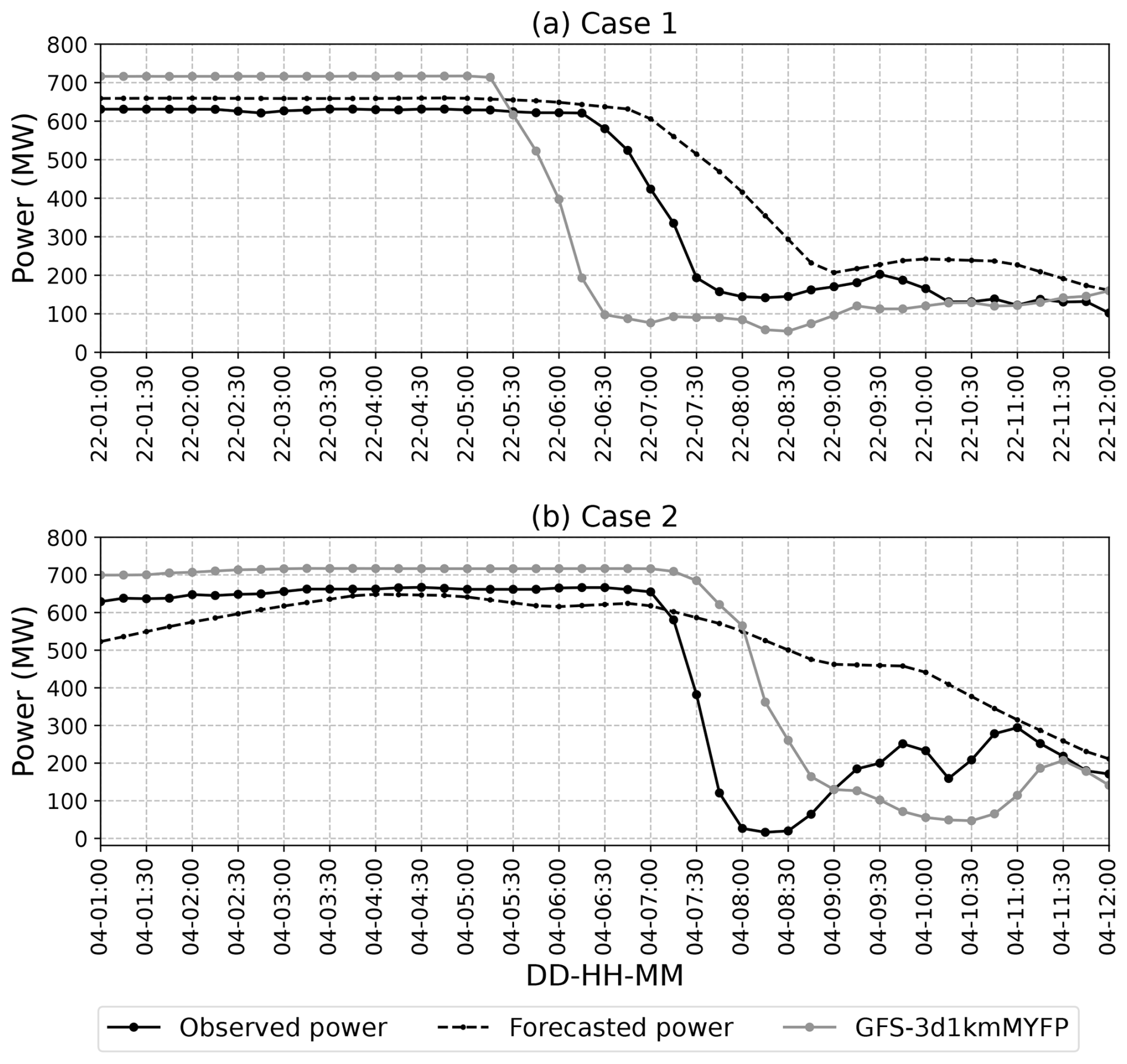
Figure 10 A comparison of wind power time series from the GFS-MYFP simulation and the Belgium offshore wind farm production and their Elia day-ahead forecast, from (a) 01:00 to 12:00 UTC on 21 February 2016 for case 1 and (b) from 01:00 to 12:00 UTC on 4 March 2016 for case 2.

The ramp statistics are computed at a 1 h timescale and are presented in Table 3. In case 1, the model-forecasted the ramp 1 h and 15 min in advance with an overestimation in intensity, whereas the Elia forecast delayed the ramp by 1 h and 15 min with an underestimation in intensity. In case 2, the model-forecasted ramp was delayed by 45 min with an underestimation in intensity, whereas no such ramp has been detected in the Elia-forecasted power (a 17 % change in 1 h is not typically considered a ramp).

To compare, the ramp intensity from the model forecasts is of a similar magnitude to that of the CERRA-2d1kmMYFP simulation for case 1 and to that of CERRA-1d1kmMYFP for case 2. This implies that extreme ramps can be forecasted well 1 d in advance, with an accuracy comparable to that of reanalysis dataset simulations.

Table 3 Overview of the ramp in wind power in terms of intensity (%) and timing (in parentheses) at a 1 h timescale, obtained from the Belgium offshore wind farm in-house day-ahead forecast and the GFS-3d1kmMYFP simulation, for cases 1 and 2. The ramp statistics from measured wind power are presented in bold text, while the best-performing simulation is italicized. All times are in UTC.

4.6 Generalization across multiple cases

So far, the results have been focused on the analysis of two cases. To generalize the robustness of the WRF model in simulating the extreme ramp events associated with FLLJs, three more cases have been simulated using configurations with CERRA IC/BCs. The synoptic charts and the measured wind power time series of these additional cases are illustrated in Figs. A1 to A3, showcasing extreme ramp events. Case 3 is simulated from 18:00 UTC on 8 February to 00:00 UTC on 10 February 2016, case 4 is simulated from 06:00 UTC on 9 January to 12:00 UTC on 10 January 2017, and case 5 is simulated from 12:00 UTC on 29 January to 18:00 UTC on 30 January 2017. A comparison between the wind-farm-measured and model-simulated wind power time series is illustrated in Fig. 11 for the three cases.

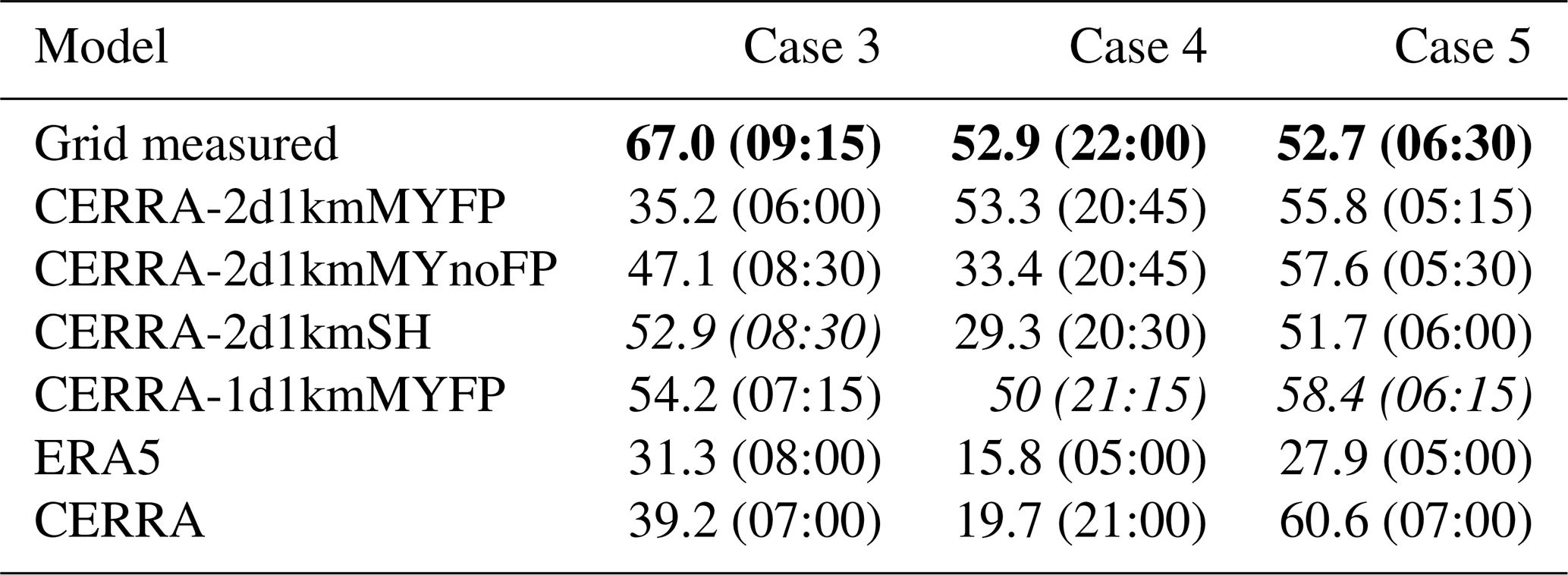
The results demonstrate that the WRF model successfully simulates the extreme wind power ramps associated with FLLJs, though the specific modeling configurations significantly influence the wind power time series. All simulations capture the strong pre-ramp wind power at the 720 MW rated capacity, likely due to peak wind speeds during the FLLJ, as well as the post-ramp wind power output, which aligns with observed values. The observed strong drop in wind power, representing the extreme ramp, is consistently simulated across cases; however, discrepancies in ramp intensity and timing persist, varying across configurations. The ramp statistics from the four CERRA-based configurations for three cases are computed at a 1 h timescale and are presented in Table 4. The CERRA-1d1kmMYFP simulation shows superior performance, with the power ramps surpassing 50 % within just 1 h, signifying the extremity of the power ramps. In terms of ramp timing, the simulated ramps are forecasted 2 h, 45 min, and 15 min in advance in cases 3, 4, and 5, respectively. This indicates the robustness of CERRA-1d1kmMYFP in accurately capturing ramp timing and intensity for cases 4 and 5. In case 3, while the timing is simulated with a 2 h lead, the ramp intensity is closely represented compared to other configurations. Other simulations exhibit larger temporal shifts in cases 4 and 5 and underpredicted intensities in cases 3 and 4. Nonetheless, these findings corroborate the robustness of the WRF model in simulating the extreme ramp events associated with the FLLJ and the better predictability of the CERRA-1d1kmMYFP modeling configuration.

Similar to cases 1 and 2, both ERA5 and CERRA significantly underestimate the ramp intensity in these additional cases, with CERRA exhibiting an overestimation in case 5. However, the ramp timings remain comparable to those obtained from the WRF simulations.

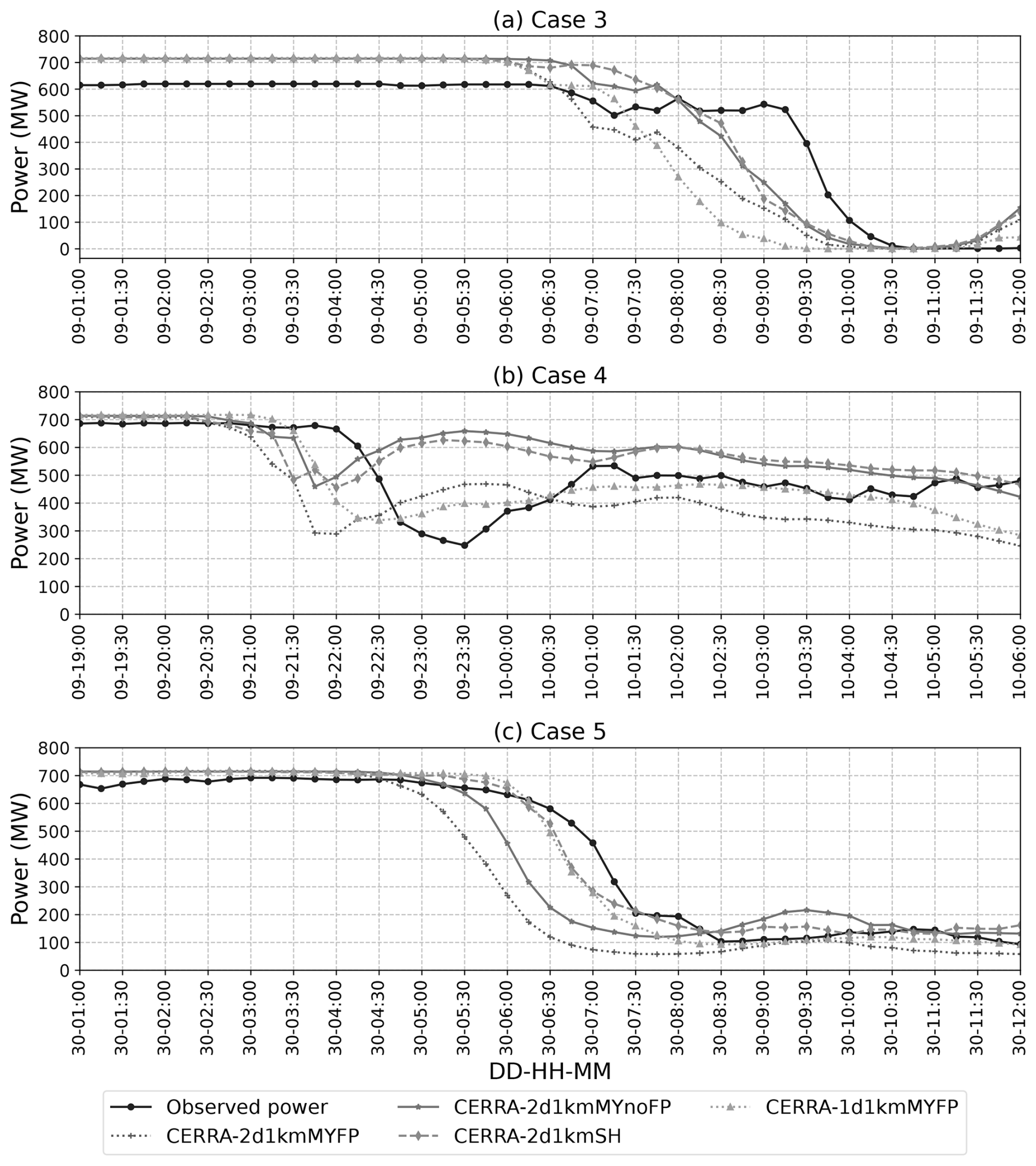
Figure 11 A comparison of wind power time series from the CERRA-2d1kmMYFP, CERRA-2d1kmMYnoFP, CERRA-2d1kmSH, and CERRA-1d1kmMYFP configurations and the Belgium offshore wind farm production. (a) From 01:00 to 12:00 UTC on 9 February 2016 for case 3. (b) From 19:00 UTC on 9 January to 06:00 UTC on 10 January 2017 for case 4. (d) From 01:00 to 12:00 UTC on 30 January 2017 for case 5.

Table 4 Overview of the ramp in wind power in terms of intensity (%) and timing (in parentheses) at a 1 h timescale, obtained from the wind power produced by the Belgium offshore wind farm and various CERRA configurations, for cases 3, 4, and 5. The ramp statistics from measured wind power are presented in bold text, while the best-performing simulation is italicized. The ramp statistics at a 60 min timescale from ERA5 and CERRA are also presented. All times are in UTC.

5 Conclusion and recommendations

In this study, we utilized the WRF model to simulate an FLLJ and associated extreme ramp events to analyze the variability in ramp timing, intensity, and jet core strength from a wind energy perspective. We identified five cases where wind power dropped by more than 50 % within 1 h at the Belgium offshore wind farm. Two of these cases were selected for in-depth analysis, while the remaining three were used for generalization. We examined the sensitivity of various model configurations, including different initial and boundary condition datasets, the activation of Fitch wind farm parameterization, and PBL schemes, to understand their impact on the FLLJ and the associated extreme ramp characteristics.

For basic climatological characterizations of FLLJs and associated extreme ramp events, the ERA5 and CERRA reanalysis datasets are highly beneficial due to their extensive coverage, long-term availability, and high accuracy. However, these datasets do not account for the wake effects of wind farms. To incorporate such effects, using the WRF model or other mesoscale models with an appropriate wind farm parameterization is recommended. Additionally, mesoscale simulations offer advanced diagnostics (e.g., turbulent kinetic energy) and, due to their high spatial resolutions, can effectively resolve coastal effects.

In this study, we found that the chosen modeling parameters significantly influence ramp characteristics and FLLJ synoptic features. The CERRA IC/BCs provided a better representation of the atmospheric flow compared to the ERA5 reanalysis, resulting in more accurate ramp timing, intensity, and FLLJ synoptic features. Activating wind farm parameterization (WFP) significantly impacted wind power output, as WFP models the interaction of individual wind turbines with the atmospheric flow and generates wind wakes in the vicinity of the wind farm. Due to wake generation, wind speeds with WFP were marginally lower than without WFP.

The scale-aware SH scheme produced a stronger FLLJ core at a higher altitude with a more defined and pronounced jet nose compared to the MYNN2.5 scheme. However, wind speeds below 200 m were lower with the SH scheme than with MYNN2.5. Finally, the single-domain configuration was more effective in simulating wind power ramp timing and intensity, consistently showing a higher core height than the nested configuration. Additionally, this configuration resulted in higher wind speeds below 200 m, leading to a more diffused jet nose profile.

Analysis of FLLJ synoptic characteristics during ramp instances revealed that the FLLJ phenomenon is primarily driven by the transect-normal wind component, aligned parallel to the frontal surface. The heightened wind ramp intensity results from the interplay between minimal transect-normal wind speed behind the front and the intensified FLLJ ahead of the front.

We observed that wind power ramp statistics can be reliably simulated using a single-domain configuration, as confirmed by three additional cases. If this approach is applicable to other FLLJs and associated extreme ramp events, it could enable accurate simulations with significantly reduced computational costs. In real-time forecasting scenarios, extreme ramp events could be predicted 1 d in advance with an accuracy comparable to reanalysis simulations, enhancing operational efficiency.

Data assimilation (DA) is a crucial factor in numerical weather prediction, particularly for real-time forecasting, where accurate initialization of model states enhances short-term predictability. As demonstrated in the studies by Wilczak et al. (2015, 2019), DA has been shown to significantly improve short-term wind power forecasts by reducing forecast biases and enhancing the representation of wind ramps. Specifically, the assimilation of in situ and remote sensing observations into high-resolution models has led to up to a 6 % reduction in RMSE for short-term wind power predictions, with notable improvements in the first few forecast hours. However, the effectiveness of DA is highly dependent on factors such as the type of observations assimilated, the assimilation technique employed, and the forecast lead time. Ivanova et al. (2025) demonstrated the benefits of four-dimensional data assimilation (FDDA) of lidar observations in improving wind speed and wind power forecasts for Belgian offshore wind farms. However, they also identified key limitations, including the dependence on specific wind directions, the scarcity of real-time offshore observations, and the restriction of FDDA to prognostic variables. While these findings reinforce the potential benefits of DA, our study had a different objective. Rather than focusing on assimilation techniques, we aimed to assess the sensitivity of modeling parameters and evaluate the WRF model's ability to simulate frontal low-level jets and extreme ramp events. In addition, we sought to improve our understanding of the underlying atmospheric processes. Future work could explore the added advantage of DA and assess its impact on extreme wind events at the resolutions and configurations considered here.

Before concluding, it is important to note that the enhanced understanding and forecasting capabilities of frontal low-level jets (FLLJs) and associated wind power ramp events extend beyond the wind energy sector. Improved insights into FLLJs are also crucial for grid operators and energy market regulators, who need to ensure system stability and manage the economic implications of sudden fluctuations in power generation.

Appendix A: Additional case studies

This section presents a wind power time series measured by the Belgium offshore wind farms during the three additional cases and the corresponding synoptic charts.

A1 Case 3

On 9 February 2016, the wind farm experienced a 67 % drop in its measured wind power within 1 h, beginning from 09:15 UTC, as shown in Fig. A1 (top panel). The farm is seen producing a maximum wind power of 600 MW for more than a 9 h period before experiencing the ramp event, suggesting the occurrence of peak wind speed during this period. Coinciding with this, the synoptic weather maps at 00:00 UTC on 9 and 10 February (bottom-left and bottom-right panels of Fig. A1, respectively) clearly illustrate a cold front (dark line with triangles pointing to the direction of frontal movement) overpassing the wind farm.

A2 Case 4

On 9 January 2017, the wind farm experienced a 52 % drop in its measured wind power within 1 h, beginning from 22:00 UTC, as shown in Fig. A2 (top panel). The farm is seen producing a maximum wind power of 690 MW for more than a 4 h period before experiencing the ramp event, suggesting the occurrence of peak wind speed during this period. Coinciding with this, the synoptic weather maps at 00:00 UTC on 9 and 10 January (bottom-left and bottom-right panels of Fig. A2, respectively) clearly illustrate a cold front (dark line with triangles pointing to the direction of frontal movement) overpassing the wind farm.

A3 Case 5

On 30 January 2017, the wind farm experienced a 52 % drop in its measured wind power within 1 h, beginning from 06:30 UTC, as shown in Fig. A3 (top panel). The farm is seen producing a maximum wind power of 670 MW for more than a 12 h period before experiencing the ramp event, suggesting the occurrence of peak wind speed during this period. Coinciding with this, the synoptic weather maps at 00:00 UTC on 30 and 31 January (bottom-left and bottom-right panels of Fig. A3, respectively) clearly illustrate a cold front (dark line with triangles pointing to the direction of frontal movement) overpassing the wind farm.

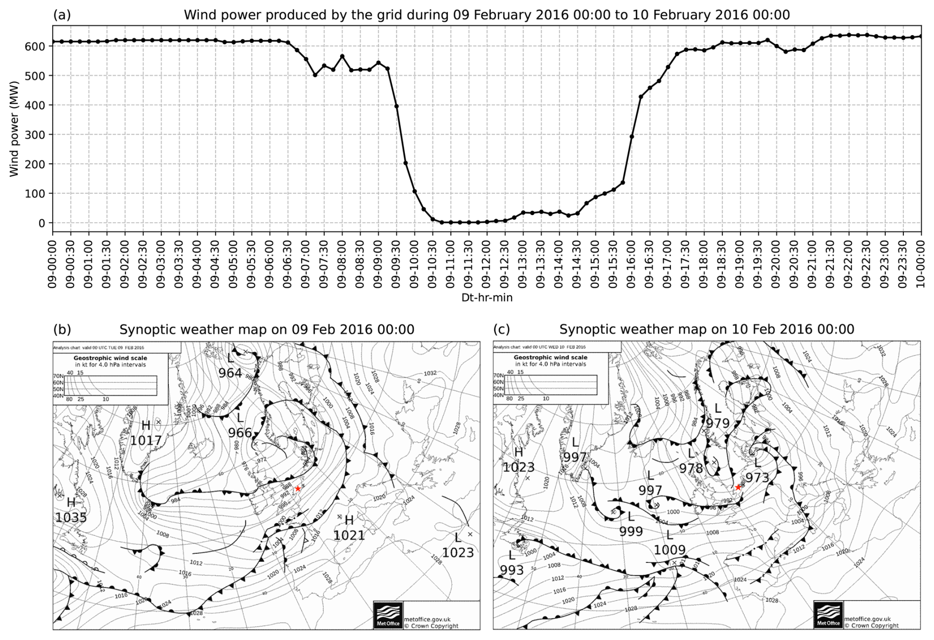
Figure A1 Same as Fig. 1 but for case 3. (a) The time series of wind power produced by the Belgian offshore wind farms, from 00:00 UTC on 9 February to 10:00 UTC on 10 February 2016, which depicts the extreme power ramp. (b) Synoptic weather maps at 00:00 UTC on 9 February 2016 and (c) 00:00 UTC on 10 February 2016, illustrating a cold front passing over the Belgium offshore wind farm (illustrated with the red star).

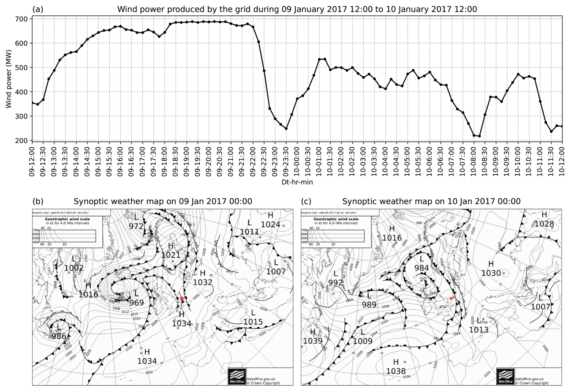
Figure A2 Same as Fig. 1 but for case 4. (a) The time series of wind power produced by the Belgian offshore wind farms, from 12:00 UTC on 9 January to 12:00 UTC on 10 January 2017, which depicts the extreme power ramp. (b) Synoptic weather maps at 00:00 UTC on 9 January 2017 and (c) 00:00 UTC on 10 January 2017, illustrating a cold front passing over the Belgium offshore wind farm (illustrated with the red star).

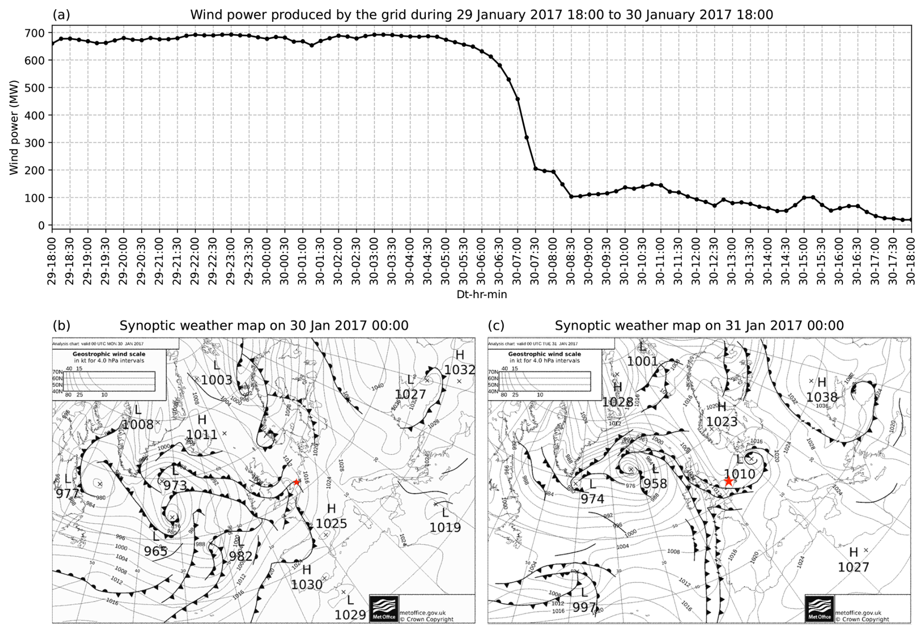
Figure A3 Same as Fig. 1 but for case 5. (a) The time series of wind power produced by the Belgian offshore wind farms, from 18:00 UTC on 29 January to 18:00 UTC on 30 January 2017, which depicts the extreme power ramp. (b) Synoptic weather maps at 00:00 UTC on 30 January 2017 and (c) 00:00 UTC on 31 January 2017, illustrating a cold front passing over the Belgium offshore wind farm (illustrated with the red star).

Appendix B: Sensitivity to the vertical levels

We have examined the influence of vertical levels on the simulations by selecting 100 vertical levels, with approximately 27 vertical levels within the first 1 km of height. Using this vertical resolution and the CERRA-1km1dMYFP configuration, the first two cases were simulated. In our study, the choice of 50 vertical levels was adopted from Nunalee and Basu (2014), where in the case of coastal LLJs, the authors reported reduced jet strength and lower jet core height with increased vertical levels, deviating from the observations. Similar to their findings, we noticed that vertical levels exert considerable influence on the ramp timing and marginal influence on the ramp intensity, as shown in Fig. B1. However, we also recognize the limitations of our findings, since they are based on two simulations focused specifically on FLLJ cases.

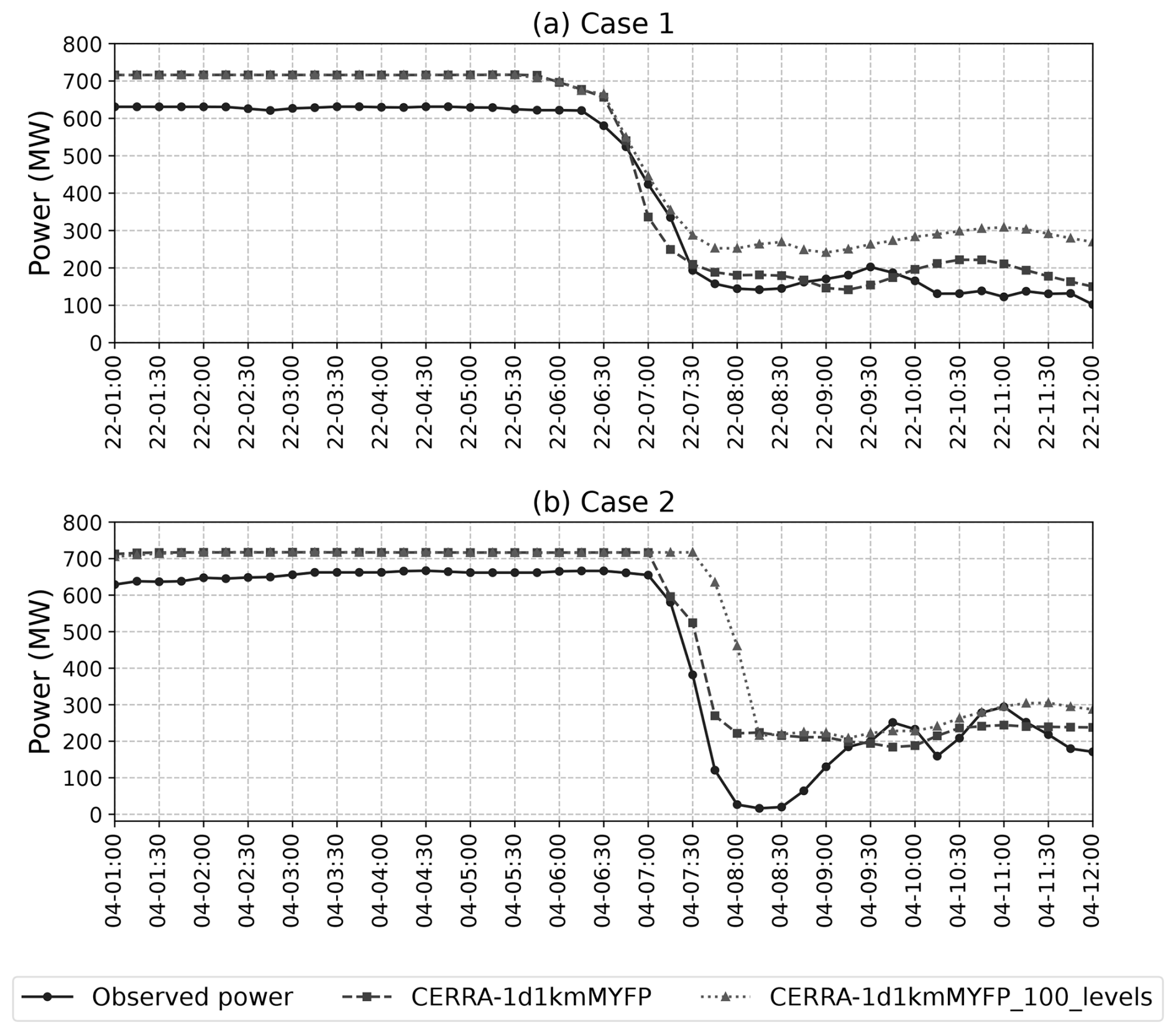
Figure B1 A comparison of wind power time series from the WRF model simulations of the CERRA-1d1kmMYFP configuration, with 50 vertical levels and 100 vertical levels, and the Belgium offshore wind farm production. (a) From 01:00 to 12:00 UTC on 21 February 2016 for case 1. (b) From 01:00 to 12:00 UTC on 4 March 2016 for case 2.

Appendix C: Sensitivity to the spin-up time

To evaluate the sensitivity of model accuracy to the choice of spin-up time, we conducted simulations for two cases using the CERRA-1d1kmMYFP configuration: one with a 6 h spin-up (original simulation duration) and another with a 12 h spin-up (starting 6 h prior to the original duration). Figure C1 presents wind power time series from both simulations compared with the measured power output for cases 1 and 2. The results show that the wind power output from both simulations is identical, indicating that a 6 h spin-up is sufficient for the development of the FLLJ cases. However, it is highly unlikely for simulations initialized with different IC/BCs to produce identical results. To further verify this, we computed the wind speed difference between the two simulations and plotted their time–height cross-section at the LOT2 location for cases 1 and 2, as shown in Fig. C2. From the illustration, it was found that the wind speed differences are infinitesimal, in the range of ±0.1 m s⁻¹ throughout and occasionally ±1 m s⁻¹; thus the wind power outputs from the two simulations also remain identical. These findings confirm that the chosen 6 h spin-up duration is adequate for accurately capturing the dynamics of these events.

Figure C1 A comparison of wind power time series from the WRF model simulations of the CERRA-1d1kmMYFP configuration, one with a 6 h spin-up and the other with a 12 h spin-up, and the Belgium offshore wind farm production. (a) From 01:00 to 12:00 UTC on 21 February 2016 for case 1. (b) From 01:00 to 12:00 UTC on 4 March 2016 for case 2.

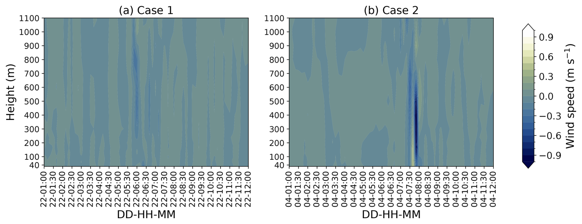
Figure C2 Time–height cross-section of wind speed difference between the CERRA-1d1kmMYFP simulations with 6 and 12 h spin-ups at the LOT2 location for cases 1 and 2.

Appendix D: Comparison between driving data

This section presents a comparison between the driving data, namely ERA5, CERRA, and GFS, for cases 1 and 2.

D1 Wind speed time series

The ERA5 reanalysis provides 100 m level wind speed at hourly intervals. In contrast, the CERRA reanalysis provides 100 m wind speed at 3-hourly analyses and hourly forecasts. To mimic a continuous hourly dataset, we procured analyses every 3 h and the forecast for the next 2 h. On the other hand, 100 m wind speed was not available in the GFS forecasts; thus we chose 975 hPa wind speed available every 3 h. A comparison between these two wind speed datasets along with the lidar observations at the LOT2 location is presented in Fig. D1.

CERRA and ERA5 provide wind speeds at 100 m above ground level, while GFS provides wind speeds at the 975 hPa pressure level. However, four of the five wind turbine types operating in the wind farm have hub heights below 100 m, making it challenging to accurately approximate wind power production using the forcing datasets. The ERA5 reanalysis exists at a temporal resolution of 1 h and a spatial resolution of 0.25°, the CERRA analysis exists at a temporal resolution of 3 h (while the forecast data have a temporal resolution of 1 h) and a spatial resolution of 5.5 km, and the GFS forecast exists at a temporal resolution of 3 h (data during 2016–2017 exist at 3-hourly intervals, while the current data are available at 1-hourly intervals) and a spatial resolution of 0.25°. Due to these coarse spatial resolutions, the entire wind farm fits within a single grid cell for ERA5 and GFS, while only a few grid cells from CERRA cover the wind farm. These spatial limitations hinder the representation of the wind power output generated by 182 turbines within the wind farm. This is critical, as the heterogeneity in turbine locations and wind conditions cannot be resolved with the coarser spatial scales of the forcing data. The GFS follows the overall trend of observed wind speeds – it exhibits a clear overestimation in magnitude. Moreover, the coarse temporal resolution of GFS makes it challenging to quantify ramp statistics, particularly as extreme ramps associated with frontal low-level jets (FLLJs) occur on scales of 15 min to 1 h. This further demonstrates that dynamical downscaling is indispensable for understanding extreme wind ramps at sub-hourly scales, which are critical for wind power applications.

D2 Wind speed profiles

The ERA5 and CERRA reanalysis datasets provide model-level wind speed data, which could serve as wind speed profiles. However, we intend to visualize the wind speed profiles from the dataset we used as IC/BCs, which are indeed pressure-level datasets. In doing so, we extracted the profiles from the metfiles of the ERA5 and CERRA runs' parent domain. The profiles are illustrated in Fig. D2 for cases 1 and 2.

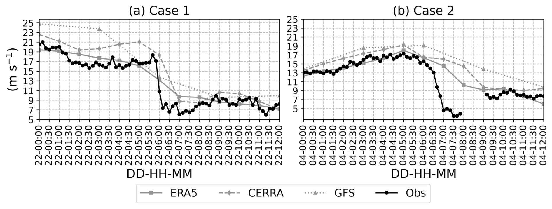
Figure D1 A comparison of 100 m wind speed time series from lidar observations, ERA5, and CERRA reanalysis. The GFS wind speed time series is extracted at a 975 hPa level. (a) From 00:00 to 12:00 UTC on 21 February 2016 for case 1. (b) From 00:00 to 12:00 UTC on 4 March 2016 for case 2.

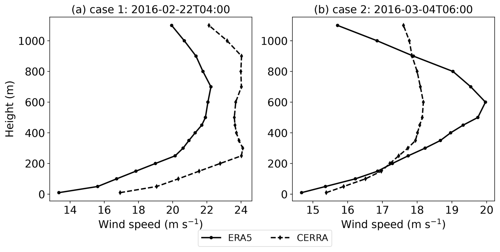
Figure D2 A comparison of wind speed profiles from the ERA5 and CERRA reanalyses for case 1 (a) at 04:00 UTC on 22 February 2016 and case 2 (b) at 06:00 UTC on 4 March 2016 at LOT2.

Appendix E: Time–height cross-section of wind speed from the WRF runs

This section presents the time–height cross-section of wind speed from the five WRF runs along with the lidar observations at the LOT2 location, for cases 1 and 2.

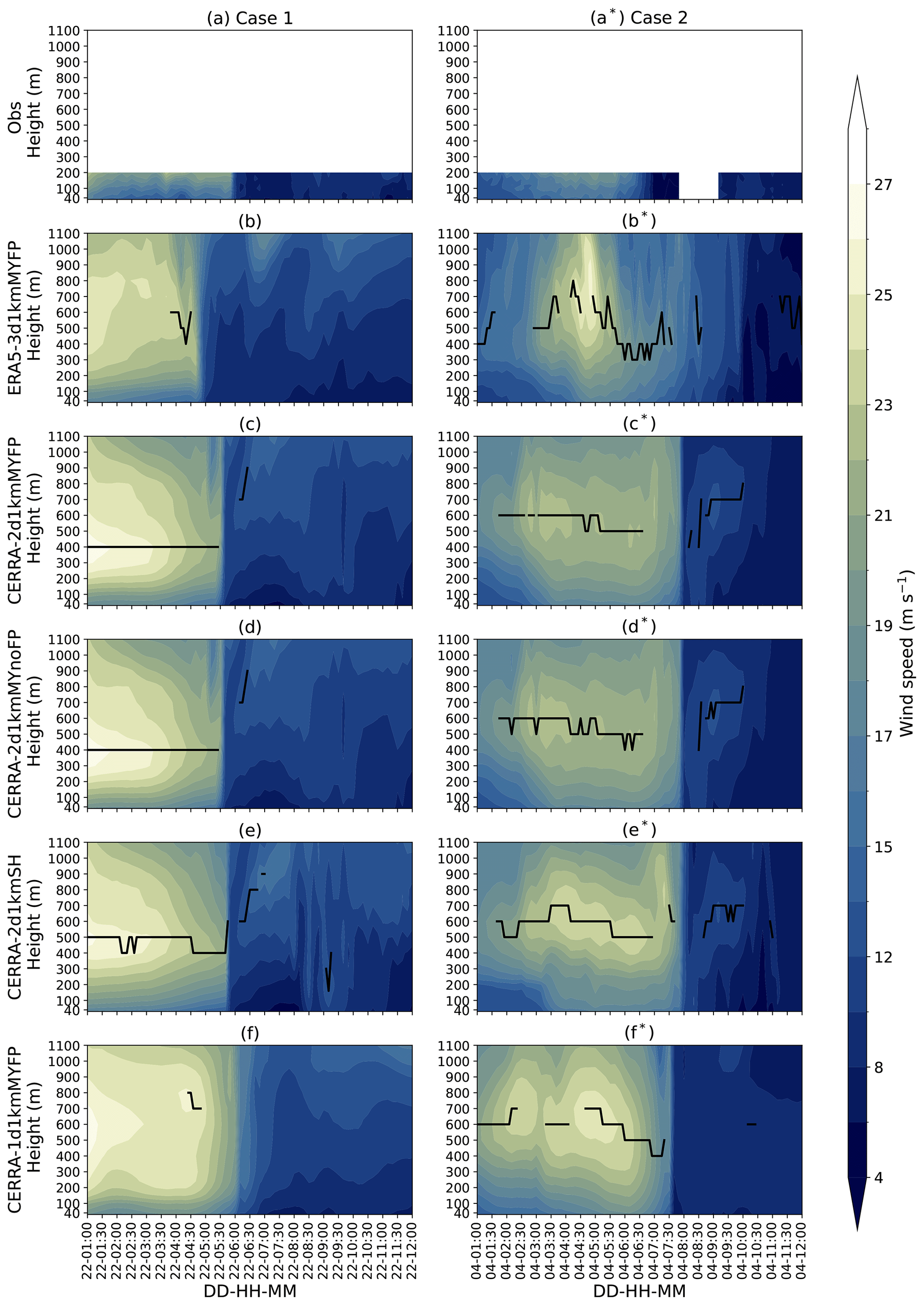
Figure E1 Time–height cross-sections of wind speed at the LOT2 location for cases 1 and 2. (a–a*) Wind speed from lidar observations. (b–b* to f–f*) Wind speed from the WRF, ERA5-3d1kmMYFP, CERRA-2d1kmMYFP, CERRA-2d1kmMYnoFP, CERRA-2d1kmSH, and CERRA-1d1kmMYFP simulations. The solid black line spanning the time series indicates the presence of a low-level jet.

Appendix F: Wind farm wakes

This section presents a comparison of horizontal wind speed contours at a 100 m level from the CERRA-2d1kmMYFP and CERRA-2d1kmMYnoFP simulations, at different time instances, for cases 1 and 2.

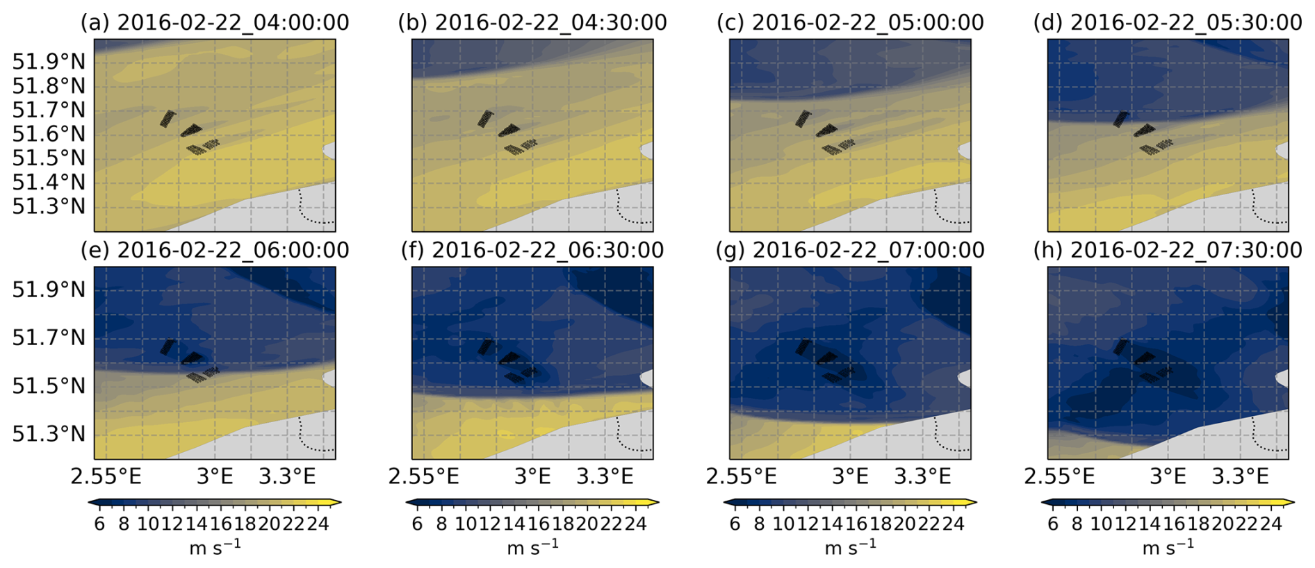
Figure F1 Illustrations of 100 m level wind speed from the CERRA-2d1kmMYFP simulation for case 1 every 30 min from 04:00 to 07:30 UTC on 22 February 2016.

Figure F2 Same as Fig. F1 but for the 2d1kmMYnoFP simulation.

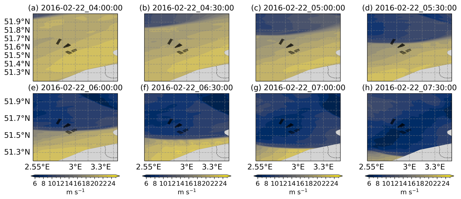
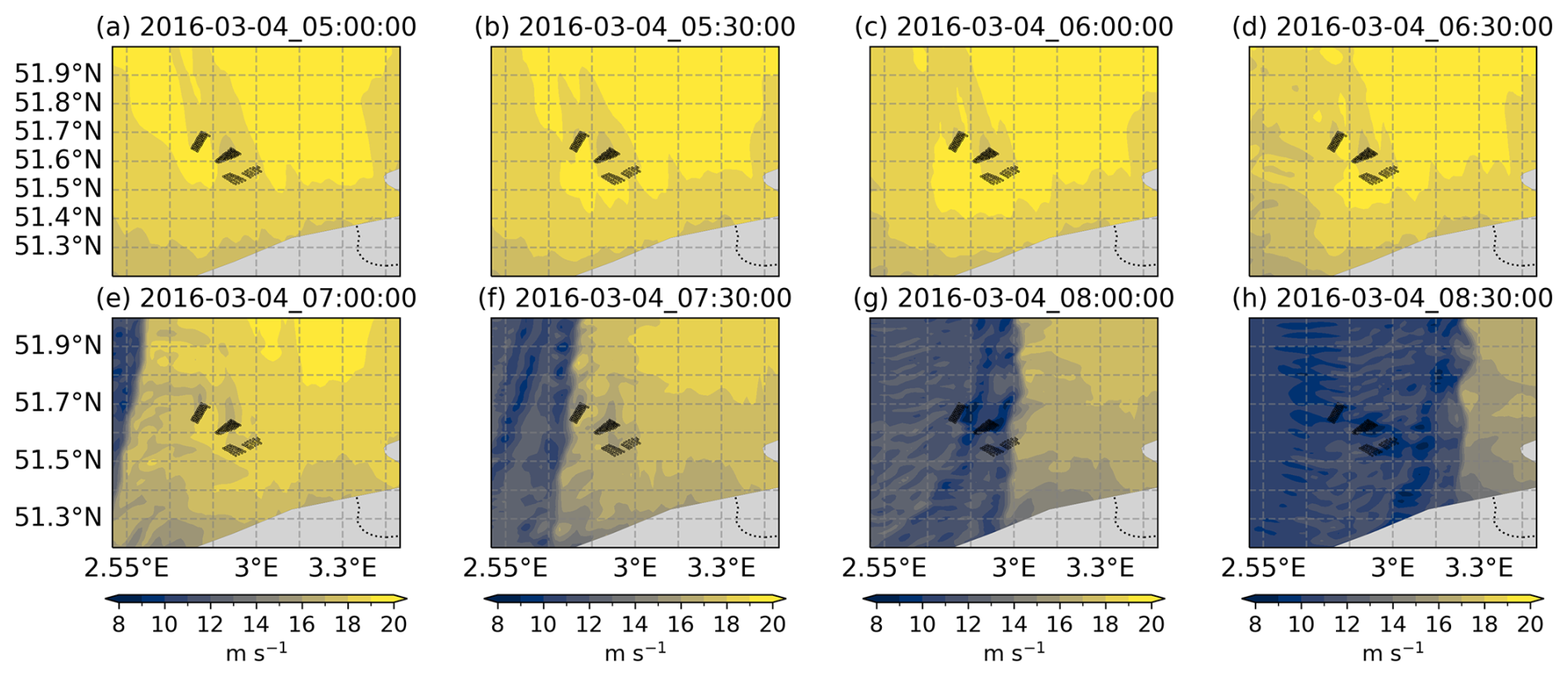
Figure F3 Illustrations of 100 m level wind speed from the CERRA-2d1kmMYFP simulation for case 2 every 30 min from 05:00 to 08:30 UTC on 4 March 2016.

Figure F4 Same as Fig. F3 but for the 2d1kmMYnoFP simulation.