Optimal control of crosswind kite systems with an engineering wake model based on vortex loops and dipoles

Modern crosswind kite systems provide a technological means to exert large aerodynamic forces in wind fields above the reach of conventional wind turbines, with applications such as airborne wind energy (AWE) generation and ship towing. A central challenge in kite system optimization is to both accurately and efficiently model self-induction effects on system design, performance, and operation. Vortex-based models are a natural candidate for this task as they provide a wake resolution that allows us to consistently capture kite-specific operating conditions. Existing vortex-based approaches have been developed under the assumption of static, axisymmetric flight, which is typically violated in practice. Therefore, we propose a vortex-based continuous-time wake model for simulation and optimal control of crosswind kites that is capable of capturing the unsteady, non-axisymmetric flight conditions induced by skewed inflow and gravity. The model represents the shed vorticity as a hybrid distribution of infinitesimal vortex loops and dipole elements and shows good agreement with simulation results obtained with the free-vortex solver DUST, with the remaining discrepancies largely due to convection-velocity selection. As a second contribution, we introduce a transcription strategy to efficiently incorporate the new model into periodic optimal control problems (OCPs). In a numerical case study based on a dual-kite system, we examine the sensitivity of the OCP optimal cost (average tether force) and design to the key transcription parameters. Based on this sensitivity analysis, we find an efficient transcription that solves the problem at three times the computational cost of the OCP without any wake model while still retaining accuracy (in terms of combined error of optimal cost and design) within 5 % compared to a highly resolved transcription of the wake-aware problem. In contrast, the solution of the no-wake problem deviates by 145 % compared to this highly resolved reference solution. Overall, the framework enables the efficient and wake-aware optimal control of crosswind kite systems and can be readily applied to industry-relevant applications such as single-kite airborne wind energy systems.

1 Introduction

Kite systems have a millennia-long history in human civilization, with significant roles in culture, science, and technology (Hart, 1982). In recent decades, advances in computing and materials science have reignited interest in these systems, motivating researchers and engineers to develop a new class of high-performance kite-based technologies. As envisaged by Loyd (1980), most of these technologies rely on soft or rigid tethered wings performing fast crosswind manoeuvers to generate substantial aerodynamic forces, which can be harnessed for various applications such as ship towing (Fritz, 2013) or electricity generation through airborne wind energy (AWE) systems (Fagiano et al., 2022). A further, yet unrealized, concept is that of airborne atmospheric actuators. Here, kite systems (without their own generation capability and thus with low complexity) could be installed strategically between wind turbines in an offshore wind farm, possibly only using existing infrastructure. By flying above the wind farm, they would be able to redirect airflow from the unaffected boundary layer into the wake of wind farms to enhance their overall efficiency through wake re-energizing. Initial simulation studies indicate that a wind farm performance boost of several percentage points could be attainable (Ploumakis and Bierbooms, 2018; Kokkedee, 2022; Van Niekerk, 2025).

One central engineering challenge for crosswind kite systems is the optimal co-design of the dynamic flight path of the kite together with its design parameters. Optimal control is a natural candidate tool for this task due to its inherent ability to deal with nonlinear constrained systems with multiple in- and outputs, which has resulted in widespread use, mainly in research (Vermillion et al., 2021) but also in industry (Noga et al., 2024). Optimal control comes with the drawback of a high computational cost and implementation effort. However, after more than a decade of research on efficient formulations and solution strategies (Horn et al., 2013; Gros et al., 2013; Malz et al., 2020; Trevisi et al., 2022) as well as open-source software developments (De Schutter et al., 2023b), it is safe to say that efficient numerical optimal control of crosswind kite systems based on high-fidelity flight mechanics is readily available for control experts and non-experts alike.

In consequence, most current research in this field focuses on improving the fidelity of the optimization models, e.g. by incorporating more realistic and flexible tether representations (Heydarnia et al., 2025) or by improving upscaling models (Joshi et al., 2024). Another major modelling challenge concerns the self-induction of the kite system. Analogous to conventional wind turbines, the aerodynamic loading of crosswind kites generates a wake that is advected downstream. This wake, in turn, induces a local wind speed deficit at the kite position, thereby diminishing the available wind power. For horizontal-axis wind turbines, this self-blockage effect has been extensively studied and establishes a theoretical upper bound on the extractable wind power, widely known as the Betz limit (Manwell et al., 2009).

Well-established induction modelling methods for horizontal-axis wind turbines are derived from momentum balance principles. However, these approaches cannot be directly applied to kite systems, as the fundamental assumptions that they rely on are typically violated. First, kite systems interact with the airflow over an annular rather than a full-disc region. Second, the aerodynamic loading is inherently non-uniform throughout a single crosswind loop. Third, the generated aerodynamic forces are often significantly misaligned with the freestream wind direction, a necessary condition to compensate for gravitational forces.

Therefore, in current engineering practice, self-induction effects are often neglected. Such a simplification is justified for existing small-scale prototypes, where relatively low aerodynamic loads act over large airborne areas. However, as system size and loading increase, and as flight trajectories are compacted to maximize power density, self-induction will become increasingly significant (Leuthold et al., 2017; Kheiri et al., 2019; Haas et al., 2019; De Schutter et al., 2023a). This effect is particularly pronounced in multi-kite configurations, where two or more wings fly tight crosswind loops around a shared main tether (Zanon et al., 2014).

Moreover, kite systems possess many degrees of freedom, and their high controllability allows them to adjust their flight path so as to avoid wake effects in consecutive flight loops, thereby boosting performance, provided that this information is incorporated in the optimization model. In conclusion, the accurate performance assessment of utility-scale kite systems requires the development of optimization-friendly engineering wake models capable of capturing self-induction effects.

Initial research efforts have primarily focused on extending momentum-based models to the kite system context by deriving analytical formulations under various simplifying assumptions: steady, axisymmetric flight (De Lellis et al., 2018; Kheiri et al., 2019; Kaufman-Martin et al., 2022); steady, non-axisymmetric flight (Akberali et al., 2021); and (unvalidated) unsteady non-axisymmetric flight conditions (Zanon et al., 2014; Leuthold et al., 2018; De Schutter et al., 2018, 2023a). However, there is currently no validated momentum-based approach available that accurately accounts for all relevant kite operating conditions. Moreover, as noted by Gaunaa et al. (2020), when using the 3D polar of the kite wing, these generalizations are physically inconsistent, leading to a double-counting of the contribution of the wake directly trailing the wing. If one would alternatively resort to a momentum approach using the 2D polar of the kite, application-specific root and tip corrections would need to be developed.

To address this last issue of consistency, Gaunaa et al. (2020), and subsequently Trevisi et al. (2023), developed physically consistent self-induction models for the steady, axisymmetric case. Their approach employed vortex methods as outlined by Branlard (2017) and demonstrated good agreement with higher-fidelity free-vortex wake simulations. A more versatile but numerically more expensive approach is offered by adding a discrete lifting-line vortex model in the transcription process of a general, unsteady AWE optimal control problem (OCP) (Leuthold et al., 2024). In the aforementioned work, reasonable agreement of the vortex model with existing large-eddy simulation (LES) results from the literature is reported. However, the computational cost of the OCP currently scales unfavourably with the number of vortex elements included, which might result in a prohibitive numerical expense in certain scenarios.

In parallel, high-fidelity approaches have been developed based on coupling the full kite flight dynamics to virtual wind environments based on LES frameworks (in some cases combined with Reynolds-averaged Navier–Stokes methods) (Haas et al., 2022; Crismer et al., 2026; Pynaert et al., 2025). While the computational expense of these methods is prohibitive for use in optimal control, the wake effects are captured implicitly through the flow solver and can be studied in great detail. In this sense, they provide the high-fidelity basis for a systematic validation of cheaper, lower-fidelity approaches, which is an interesting direction for the future. One current limitation of these methods is that they rely on flight trajectories that are generated without a wake model. This further highlights the need for reduced-order, optimization-friendly wake models that consistently account for self-induction effects.

The contribution of this paper is the formulation of a new optimization-friendly, vortex-based self-induction wake model that is capable of capturing the inherently unsteady and non-axisymmetric operating conditions of kite systems. Rather than deriving a simplified analytical approximation or employing a discrete vortex model, we represent the coupled dynamics of the kite system and its wake continuously through a combined differential-algebraic equation (DAE) and partial differential equation (PDE) framework. The resulting continuous model is validated in relevant conditions against the higher-fidelity free-vortex wake solver DUST. Finally, we demonstrate how the DAE- and PDE-based OCP can be efficiently transcribed into a standard continuous-time OCP formulation and analyse the sensitivity of the resulting problem to key transcription parameters.

To limit the scope of this paper, we consider a kite system with fixed tether length, thereby excluding pumping-style AWE systems, which rely on tether reeling. The kite system is also not equipped with on-board power generators, acting purely as an actuator. However, the developed methods in this paper can be directly applied to pumping- or fly-gen-type systems as well. In fact, due to their unsteady nature, these methods are particularly suited for capturing pumping wake patterns, including build-up during reel-out and reset due to reel-in. We focus here on a dual-kite system model to generate an interesting high-load scenario with significant induction effects. Similarly, application of the developed methods to single-kite systems is straightforward.

The remainder of this paper is organized as follows. Section 2 introduces the DAE model of a multi-kite system as described in the literature. Section 3 presents the vortex-based continuous wake model and its associated PDE dynamics. In Sect. 4, we present validation results by comparing model simulations with those from the free-vortex simulation framework DUST. Section 5 then formulates the coupled DAE–PDE OCP and discusses its efficient transcription into a continuous-time OCP form. Section 6 presents the results of a representative numerical case study. Finally, Sect. 7 provides a conclusion and outlines possible directions for future research.

Figure 1 Illustration of the dual-wing crosswind kite system considered in this paper.

2 Kite system model

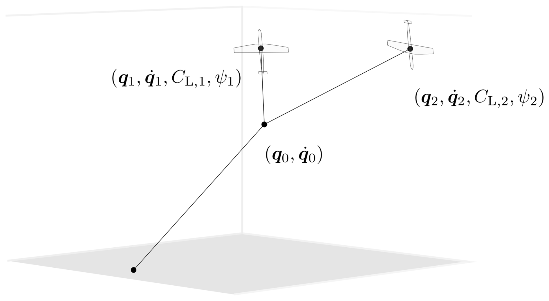
In this section, we present the flight dynamics model of a dual-kite system as shown in Fig. 1. The model is largely synthesized from the literature. As argued by Gros and Diehl (2013), for optimal control applications, it is beneficial to model the flight dynamics of tethered airfoils by an index-1 DAE such as

$$\begin{array}{}\text{(1)}& \mathit{F}\left(\mathit{x}\right(t),\dot{\mathit{x}}(t),\mathit{u}(t),\mathit{z}(t),\mathit{y}(t,\cdot ),\mathit{\theta })=\mathrm{0},\forall t\in \mathbb{R},\end{array}$$

with states x(t), controls u(t), algebraic variables z(t), and design parameters θ. Here, we introduce the wake representation y(t,τ) as a new element.

The full wake state $\mathit{y}(t,\cdot )$ represents the overall spatial vorticity distribution (e.g. structure, orientation, strength) that has resulted from the flight trajectory up until the current physical time t. The wake state y(t,τ) then represents an infinitesimal segment of this distribution, which has an age (or convection time) $\mathit{\tau }\in {\mathbb{R}}^{+}$, which represents the time elapsed since that portion of the wake was generated at the boundary τ=0. The evolution of the wake is described by the inhomogeneous transport equation

$$\begin{array}{}\text{(2)}& {\displaystyle \frac{\mathrm{d}\mathit{y}}{\mathrm{d}t}}(t,\mathit{\tau })+{\displaystyle \frac{\mathrm{d}\mathit{y}}{\mathrm{d}\mathit{\tau }}}(t,\mathit{\tau })=\mathit{f}\left(\mathit{y}\right(t-\mathit{\tau },\cdot \left)\right),\forall (t,\mathit{\tau })\in {\mathbb{R}}^{\mathrm{2}},\end{array}$$

with the boundary condition

$$\begin{array}{}\text{(3)}& \mathit{y}(t,\mathrm{0})=\mathit{g}\left(\mathit{x}\right(t),\mathit{y}(t,\cdot \left)\right),\forall t\in \mathbb{R}.\end{array}$$

Thus, overall, the kite system dynamics are described by a coupled DAE–PDE system. In this section, we focus solely on the DAE part of the dynamics. Section 3 then later describes the wake parameterization y(t,τ), source term function f, and boundary condition function g in detail.

2.1 Dual-wing flight dynamics

While high-fidelity 6DOF aircraft models are available in the literature and open-source software, we limit ourselves here to the more simple point-mass model as proposed by Zanon et al. (2013). The state, control, and algebraic variables are defined as

$$\begin{array}{}\text{(4)}& \mathit{x}:=(\mathit{q},\dot{\mathit{q}},C_{\mathrm{L}},\mathit{\psi }),\mathit{u}:=({\dot{C}}_{\mathrm{L}},\dot{\mathit{\psi }}),\mathit{z}:=\mathit{\lambda },\end{array}$$

where $\mathit{q}:=({\mathit{q}}_{\mathrm{0}},{\mathit{q}}_{\mathrm{1}},{\mathit{q}}_{\mathrm{2}})\in {\mathbb{R}}^{\mathrm{9}}$ are the positions of the centre point and the two wings, and C_L∈ℝ² are the lift coefficients and ψ∈ℝ² the roll angles of the two wings. The algebraic variables λ∈ℝ³ are the Lagrange multipliers associated with the holonomic constraints

$$\begin{array}{}\text{(5)}& \mathit{c}(\mathit{x},\mathit{\theta }):={\displaystyle \frac{\mathrm{1}}{\mathrm{2}}}\left[\begin{array}{c}{\mathit{q}}_{\mathrm{0}}^{\top }{\mathit{q}}_{\mathrm{0}}-l_{\mathrm{t}}^{\mathrm{2}}\\ ({\mathit{q}}_{\mathrm{1}}-{\mathit{q}}_{\mathrm{0}}{)}^{\top }({\mathit{q}}_{\mathrm{1}}-{\mathit{q}}_{\mathrm{0}})-l_{\mathrm{s}}^{\mathrm{2}}\\ ({\mathit{q}}_{\mathrm{2}}-{\mathit{q}}_{\mathrm{0}}{)}^{\top }({\mathit{q}}_{\mathrm{2}}-{\mathit{q}}_{\mathrm{0}})-l_{\mathrm{s}}^{\mathrm{2}}\end{array}\right]=\mathrm{0},\end{array}$$

which impose that the node positions are consistent with the tether lengths l_t∈ℝ and l_s∈ℝ of the main and secondary tethers, respectively. These parameters, together with the corresponding tether diameters d_t∈ℝ and d_s∈ℝ, can be optimized and are summarized in the parameter vector

$$\begin{array}{}\text{(6)}& \mathit{\theta }:=(l_{\mathrm{t}},l_{\mathrm{s}},d_{\mathrm{t}},d_{\mathrm{s}}).\end{array}$$

Using the Lagrangian mechanics with index reduction approach proposed by Gros and Diehl (2013) and implemented by De Schutter et al. (2023b), we can derive the following equations of motion:

$$\begin{array}{}\text{(7)}& {\displaystyle }\left[\begin{array}{cc}\mathbf{M}& {\mathrm{\nabla }}_{\mathit{q}}\mathit{c}\\ {\mathrm{\nabla }}_{\mathit{q}}{\mathit{c}}^{\top }& \mathrm{0}\end{array}\right]\left[\begin{array}{c}\ddot{\mathit{q}}\\ \mathit{\lambda }\end{array}\right]={\mathit{F}}_{\mathrm{ext}}\end{array}$$

with the mass matrix

$$\begin{array}{}\text{(8)}& \mathbf{M}:=\left[\begin{array}{ccc}{\mathbf{M}}_{\mathrm{t}}+\mathrm{2}{\mathbf{M}}_{\mathrm{s}}& \frac{\mathrm{1}}{\mathrm{2}}{\mathbf{M}}_{\mathrm{s}}& \frac{\mathrm{1}}{\mathrm{2}}{\mathbf{M}}_{\mathrm{s}}\\ \frac{\mathrm{1}}{\mathrm{2}}{\mathbf{M}}_{\mathrm{s}}& {\mathbf{M}}_{\mathrm{s}}+m_{\mathrm{w}}{\mathbf{I}}_{\mathrm{3}}& \mathrm{0}\\ \frac{\mathrm{1}}{\mathrm{2}}{\mathbf{M}}_{\mathrm{s}}& \mathrm{0}& {\mathbf{M}}_{\mathrm{s}}+m_{\mathrm{w}}{\mathbf{I}}_{\mathrm{3}}\end{array}\right],\end{array}$$

where m_w is the wing mass, and the terms ${\mathbf{M}}_{\mathrm{t}}:=\frac{\mathrm{1}}{\mathrm{3}}{\mathit{\mu }}_{\mathrm{t}}{l}_{\mathrm{t}}{\mathbf{I}}_{\mathrm{3}}$ and ${\mathbf{M}}_{\mathrm{s}}:=\frac{\mathrm{1}}{\mathrm{3}}{\mathit{\mu }}_{\mathrm{s}}{l}_{\mathrm{s}}{\mathbf{I}}_{\mathrm{3}}$ are used to describe the inertia of the tether. The density per unit length of the tether lengths is a function of the tether diameter, i.e. ${\mathit{\mu }}_{\mathrm{t}}:={\mathit{\rho }}_{\mathrm{t}}\frac{\mathit{\pi }{d}_{\mathrm{t}}^{\mathrm{2}}}{\mathrm{4}}$ and ${\mathit{\mu }}_{\mathrm{s}}:={\mathit{\rho }}_{\mathrm{t}}\frac{\mathit{\pi }{d}_{\mathrm{s}}^{\mathrm{2}}}{\mathrm{4}}$, with ρ_t being the material density.

The external force vector is given as

$$\begin{array}{}\text{(9)}& {\mathit{F}}_{\mathrm{ext}}:=\left[\begin{array}{c}{\mathit{F}}_{\mathrm{0}}-\frac{\mathrm{3}}{\mathrm{2}}g({\mathbf{M}}_{\mathrm{t}}+\mathrm{2}{\mathbf{M}}_{\mathrm{s}}){\mathit{e}}_z\\ {\mathit{F}}_{\mathrm{1}}-g(m_{\mathrm{w}}{\mathbf{I}}_{\mathrm{3}}+\frac{\mathrm{3}}{\mathrm{2}}{\mathbf{M}}_{\mathrm{s}}){\mathit{e}}_z\\ {\mathit{F}}_{\mathrm{2}}-g(m_{\mathrm{w}}{\mathbf{I}}_{\mathrm{3}}+\frac{\mathrm{3}}{\mathrm{2}}{\mathbf{M}}_{\mathrm{s}}){\mathit{e}}_z\\ -{\mathrm{\nabla }}_{\dot{\mathit{q}}}{\dot{\mathit{c}}}^{\top }\dot{\mathit{q}},\end{array}\right]\end{array}$$

with F₀, F₁, and F₂ being the aerodynamic forces. In the implementation, Baumgarte stabilization is added in the last element of this vector to ensure consistency of the solution in the context of periodic optimal control (Gros and Zanon, 2018).

2.2 Aerodynamics

To compute the aerodynamic forces, we assume a uniform free-stream wind speed u_∞∈ℝ³ and constant density ρ∈ℝ. Alternatively, realistic wind shear and density drop profiles can be incorporated as well in a straightforward fashion. Within the proposed framework of Sect. 3, the modelled wind shear would be taken into account automatically in the wake development. Within the scope of this paper, we limit ourselves to validating the model in uniform inflow conditions.

The wake state $\mathit{y}(t,\cdot )$ induces a velocity field ${\mathit{u}}_i^{\mathrm{f}}\left({\mathit{q}}_i\right(t),\mathit{y}(t,\cdot \left)\right)$ on top of the free-stream wind, resulting in a total wind field ${\mathit{u}}_{\mathrm{t},i}\left({\mathit{q}}_i\right(t),\mathit{y}(t,\cdot \left)\right)$, which is evaluated at each of the wing positions q_i(t) for $i\in \mathit{\{}\mathrm{1},\mathrm{2}\mathit{\}}$:

$$\begin{array}{}\text{(10)}& {\mathit{u}}_{\mathrm{t},i}\left({\mathit{q}}_i\right(t),\mathit{y}(t,\cdot \left)\right):={\mathit{u}}_{\mathrm{\infty }}+{\mathit{u}}_i^{\mathrm{f}}\left({\mathit{q}}_i\right(t),\mathit{y}(t,\cdot \left)\right).\end{array}$$

For an explicit definition of the induced velocity functions ${\mathit{u}}_i^{\mathrm{f}}$, we refer to Sect. 3.

The apparent wind speed seen by each wing is then given by

$$\begin{array}{}\text{(11)}& {\mathit{u}}_{\mathrm{a},i}:={\mathit{u}}_{\mathrm{t},i}\left({\mathit{q}}_i\right(t),\mathit{y}(t,\cdot \left)\right)-{\dot{\mathit{q}}}_i\left(t\right),i\in \mathit{\{}\mathrm{1},\mathrm{2}\mathit{\}},\end{array}$$

where, for notational simplicity, we further omit the explicit dependence on time.

Then, assuming no side-slip and direct control of the roll angle ψ_i of the wings, the resulting lift and drag forces are given by

$$\begin{array}{ll}{\displaystyle }{\mathit{F}}_{\mathrm{L},i}& {\displaystyle }:={\displaystyle \frac{\mathrm{1}}{\mathrm{2}}}\mathit{\rho }{S}_{\mathrm{w}}{C}_{\mathrm{L},i}\left|\right|{\mathit{u}}_{\mathrm{a},i}\left|{|}^{\mathrm{2}}\right(\cos \left({\mathit{\psi }}_i\right){\mathit{e}}_{\mathrm{L},i}-\sin \left({\mathit{\psi }}_i\right){\mathit{e}}_{\mathrm{T},i})\\ {\displaystyle }{\mathit{F}}_{\mathrm{D},i}& {\displaystyle }:={\displaystyle \frac{\mathrm{1}}{\mathrm{2}}}\mathit{\rho }{S}_{\mathrm{w}}{C}_{\mathrm{D},i}\left|\right|{\mathit{u}}_{\mathrm{a},i}\left|\right|{\mathit{u}}_{\mathrm{a},i},\end{array}$$

with the vectors e_L,i and e_T,i defined by

$$\begin{array}{}\text{(12)}& {\mathit{e}}_{\mathrm{T},i}:={\displaystyle \frac{{\mathit{u}}_{\mathrm{a},i}\times {\mathit{e}}_{\mathrm{r},i}}{\left|\right|{\mathit{u}}_{\mathrm{a},i}\times {\mathit{e}}_{\mathrm{r},i}\left|\right|}},{\mathit{e}}_{\mathrm{L},i}:={\displaystyle \frac{{\mathit{e}}_{\mathrm{T},i}\times {\mathit{u}}_{\mathrm{a},i}}{\left|\right|{\mathit{e}}_{\mathrm{T},i}\times {\mathit{u}}_{\mathrm{a},i}\left|\right|}},\end{array}$$

where e_r,i is the tether direction

$$\begin{array}{}\text{(13)}& {\mathit{e}}_{\mathrm{r},i}:={\displaystyle \frac{{\mathit{q}}_i-{\mathit{q}}_{\mathrm{0}}}{\left|\right|{\mathit{q}}_i-{\mathit{q}}_{\mathrm{0}}\left|\right|}}.\end{array}$$

The aerodynamic drag coefficient includes the induced-drag term of an elliptical wing in straight flight:

$$\begin{array}{}\text{(14)}& C_{\mathrm{D},i}:=C_{\mathrm{D},\mathrm{0}}+{\displaystyle \frac{C_{\mathrm{L},i}^{\mathrm{2}}}{\mathit{\pi }\mathrm{AR}}},\end{array}$$

with C_D,0 being the parasitic drag and AR the aspect ratio. Note that the induced-drag term approximates the effect of the velocities induced by the part of the wake directly trailing the wing. This will be taken into account in the wake model in Sect. 3 so as to avoid double-counting, similar to Trevisi et al. (2023).

The overall aerodynamic forces are given as

$$\begin{array}{}\text{(15)}& {\displaystyle }{\mathit{F}}_{\mathrm{0}}& {\displaystyle }={\mathit{F}}_{\mathrm{t},\mathrm{0}}\text{(16)}& {\displaystyle }{\mathit{F}}_i& {\displaystyle }={\mathit{F}}_{\mathrm{L},i}+{\mathit{F}}_{\mathrm{D},i}+{\mathit{F}}_{\mathrm{t},i},i\in \mathit{\{}\mathrm{1},\mathrm{2}\mathit{\}},\end{array}$$

where F_t,i values are the tether drag forces, proportional to the tether lengths and diameters. For each tether, these forces are computed for the boundary nodes such that they produce resultant forces and moments equivalent to those obtained by numerically integrating the drag distribution along the tether. To simplify the exposition, we refer to De Schutter et al. (2023b, Eq. 36) for the explicit expressions.

3 Continuous wake modelling

We start our exposition of the continuous wake model by assuming that the two wings each have their own separate trailing wake described by the states ${\mathit{y}}_{\mathrm{1}}(t,\mathit{\tau })\in {\mathbb{R}}^{n_y}$ and ${\mathit{y}}_{\mathrm{2}}(t,\mathit{\tau })\in {\mathbb{R}}^{n_y}$, respectively, which are combined to form a total wake state:

$$\begin{array}{}\text{(17)}& \mathit{y}(t,\mathit{\tau }):=\left[\begin{array}{c}{\mathit{y}}_{\mathrm{1}}(t,\mathit{\tau })\\ {\mathit{y}}_{\mathrm{2}}(t,\mathit{\tau })\end{array}\right].\end{array}$$

This wake state is the unique solution to the initial value problem defined by Eqs. (2) and (3). This solution can be explicitly expressed for each wake state $i\in \mathit{\{}\mathrm{1},\mathrm{2}\mathit{\}}$ in terms of the functions f_i and g_i:

$$\begin{array}{}\text{(18)}& {\mathit{y}}_i(t,\mathit{\tau }):={\mathit{g}}_i\left(\mathit{x}\right(t-\mathit{\tau }),\mathit{y}(t-\mathit{\tau },\cdot \left)\right)+\underset{\mathrm{0}}{\overset{\mathit{\tau }}{\int }}{\mathit{f}}_i\left(\mathit{y}\right(t-\mathit{\tau },\cdot \left)\right)\mathrm{d}s.\end{array}$$

The forcing terms f_i(t,τ) can be used to model the wake convection and effects such as viscous dissipation and radial expansion. Within the scope of this paper, we assume rigid convection with a velocity assigned at the moment of shedding. The functions g_i model the vortex properties at the moment of shedding, which depend on the system state and on the entire vortex structure itself (via the induced velocities).

The induced velocity evaluated at the position of each wing q_i is the superposition of the induced velocities of the individual wakes. These velocities are computed as an integral over the entire wake structure, assuming an infinitely long wake. For each wing, we ignore the induction of its own trailing wake less than a time T away (“near” wake) and instead account for these near-wing effects through the induced-drag term. Accurately resolving this region would require a significantly finer representation of the vortex distribution close to the wing, increasing model complexity and computational cost. Beyond the time T (“far” wake), we assume that the shed vorticity has rolled up into two trailing vortices. Therefore, we arrive at the following expression for the induced velocities for wing 1:

$$\begin{array}{}\text{(19)}& \begin{array}{rl}{\mathit{u}}_{\mathrm{1}}^{\mathrm{f}}\left({\mathit{q}}_{\mathrm{1}}\right(t),\mathit{y}(t,\cdot \left)\right)& :=\underset{T}{\overset{\mathrm{\infty }}{\int }}{\mathit{u}}^{\prime }\left({\mathit{q}}_{\mathrm{1}}\right(t),{\mathit{y}}_{\mathrm{1}}(t,\mathit{\tau }\left)\right)\mathrm{d}\mathit{\tau }\\ & +\underset{\mathrm{0}}{\overset{\mathrm{\infty }}{\int }}{\mathit{u}}^{\prime }\left({\mathit{q}}_{\mathrm{1}}\right(t),{\mathit{y}}_{\mathrm{2}}(t,\mathit{\tau }\left)\right)\mathrm{d}\mathit{\tau }\end{array}\end{array}$$

and vice versa for wing 2.

Thus, to define a wake model in this framework, one must define a wake state representation y_i and the corresponding forcing and shedding functions f_i and g_i and then model the induced velocity with the function u^′.

3.1 Continuous vortex-loop model

We propose to model each wake structure ${\mathit{y}}_i(t,\cdot )$ as a continuous trail of infinitely small vortex rectangles made up of infinitely thin vortex filaments with variable circulation strength Γ_i(t,τ), as shown in Fig. 2 (left). The pair of chordwise vortex filaments with infinitesimal length ds model the rolled-up wing tip vortices. The wake is shed with the apparent wind speed; hence the infinitesimal length can also be written as a function of τ as $\mathrm{d}s:=\left|\right|{\mathit{u}}_{\mathrm{a},i}(t-\mathit{\tau })\left|\right|\mathrm{d}\mathit{\tau }$. We assume that these chordwise filaments are located at a distance of $\frac{\mathit{\pi }}{\mathrm{4}}b$ from each other (Gaunaa et al., 2020), symmetric relative to the rectangle centre position ${\mathit{q}}_{\mathrm{v},i}(t,\mathit{\tau })$. This distance equals the length of the pair of spanwise vortex filaments, which capture the shed vorticity caused by the variation in lift force over time. The orientation of the rectangles is determined by the normal unit vector ${\mathit{e}}_{\mathrm{n},i}(t,\mathit{\tau })$ and chordwise unit vector ${\mathit{e}}_{\mathrm{c},i}(t,\mathit{\tau })$. The wake states are then defined as

$$\begin{array}{}\text{(20)}& {\mathit{y}}_i(t,\mathit{\tau }):=\left[\begin{array}{c}{\mathit{q}}_{\mathrm{v},i}(t,\mathit{\tau })\\ {\mathrm{\Gamma }}_i(t,\mathit{\tau })\\ {\mathit{e}}_{\mathrm{n},i}(t,\mathit{\tau })\\ {\mathit{e}}_{\mathrm{c},i}(t,\mathit{\tau })\end{array}\right].\end{array}$$

For the forcing term, we assume rigid downstream convection with a velocity ${\mathit{u}}_{\mathrm{conv},i}\left(\mathit{y}\right(t-\mathit{\tau },\cdot \left)\right)\in {\mathbb{R}}^{\mathrm{3}}$. This assumption implies that the shed wake elements are transported without deformation or dissipation:

$$\begin{array}{}\text{(21)}& {\mathit{f}}_i\left(y\right(t-\mathit{\tau },\cdot \left)\right):=\left[\begin{array}{c}{\mathit{u}}_{\mathrm{conv},i}\left(\mathit{y}\right(t-\mathit{\tau },\cdot \left)\right)\\ {\mathrm{0}}_{\mathrm{7}\times \mathrm{1}}\end{array}\right].\end{array}$$

In reality, the wake evolution results from complex vortex–vortex interactions and self-induced deformations, which are computationally prohibitive to resolve explicitly. To account for these effects in a tractable manner, Sect. 4 introduces and compares three heuristic strategies for selecting the convection velocity.

The shedding laws g_i are defined such that the shed rectangle centre positions ${\mathit{q}}_{\mathrm{v},i}(t,\mathrm{0})$ coincide with the wings' aerodynamic centre, here assumed equal to the centre of mass positions q_i(t). The trailing vortex strength Γ_i(t,0) follows from the Kutta–Joukowski theorem (Gaunaa et al., 2020; Trevisi et al., 2023) for elliptic wings, while the rectangle unit vectors ${\mathit{e}}_{\mathrm{n},i}(t,\mathrm{0})$ and ${\mathit{e}}_{\mathrm{c},i}(t,\mathrm{0})$ are aligned with the lift force and apparent wind speed, respectively, which are orthogonal by definition:

$$\begin{array}{}\text{(22)}& {\mathit{g}}_i\left(\mathit{x}\left(t\right),\mathit{y}(t,\cdot )\right):=\left[\begin{array}{c}{\mathit{q}}_i\left(t\right)\\ \frac{\mathrm{2}b}{\mathit{\pi }\mathrm{AR}}{C}_{\mathrm{L},i}\left(t\right)\left|\right|{\mathit{u}}_{\mathrm{a},i}\left(t\right)\left|\right|\\ \frac{{\mathit{F}}_{\mathrm{L},i}\left(t\right)}{\left|\right|{\mathit{F}}_{\mathrm{L},i}\left(t\right)\left|\right|}\\ \frac{{\mathit{u}}_{\mathrm{a},i}\left(t\right)}{\left|\right|{\mathit{u}}_{\mathrm{a},i}\left(t\right)\left|\right|}\end{array}\right].\end{array}$$

Finally, the induced velocity at a position $\widehat{\mathit{q}}\in {\mathbb{R}}^{\mathrm{3}}$ by an infinitesimally small rectangle per unit width $\mathrm{d}s=\left|\right|{\mathit{u}}_{\mathrm{a}}(t-\mathit{\tau })\left|\right|\mathrm{d}\mathit{\tau }$ is given by

$$\begin{array}{}\text{(23)}& {\mathit{u}}^{\prime }\left(\widehat{\mathit{q}}\right(t),{\mathit{y}}_i(t,\mathit{\tau }\left)\right):={\left.{\displaystyle \frac{\mathrm{d}{\mathit{u}}_{\mathrm{vl}}(\widehat{\mathit{q}},{\mathit{y}}_i(t,\mathit{\tau }),\mathrm{\Delta }s)}{\mathrm{d}\mathrm{\Delta }s}}\right|}_{\mathrm{\Delta }s=\mathrm{0}}\left|\right|{\mathit{u}}_{\mathrm{a},i}(t-\mathit{\tau })\left|\right|,\end{array}$$

where the function u_vl computes the velocity induced by a rectangular vortex loop of chordwise extent Δs, obtained from the Biot–Savart law applied to its four bounding vortex filaments, as written out in Appendix A.

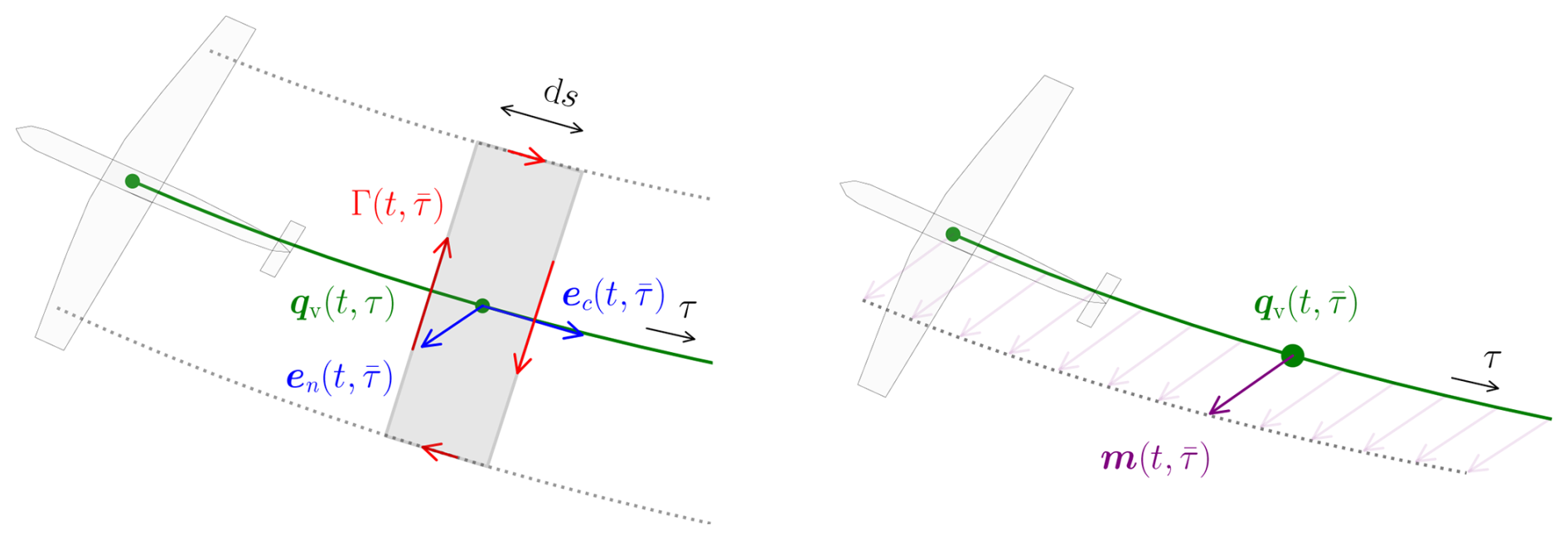
Figure 2 Illustration of the continuous wake representation based on rectangular vortex loops with the infinitesimally small width $\mathrm{d}s:=\parallel {\mathit{u}}_{\mathrm{a}}(t-\mathit{\tau })\parallel \mathrm{d}\mathit{\tau }$ (left) and of the wake representation based on a continuous trail of vortex dipoles (right).

3.2 Continuous vortex dipole model

The symbolic complexity of Eq. (23) is relatively high, leading to expensive numerical derivatives and a high memory usage. This complexity can be reduced by applying a multi-pole expansion of the infinitesimal vortex loops and retaining only the leading non-vanishing term, which gives us a far-field approximation of the original induced velocity. This approximation can be interpreted as the induced velocity of a source dipole whose dipole moment is proportional to the enclosed area of the rectangular vortex loop.

Thus, we can also model the wake state as a continuous trail of vortex dipoles, visualized in Fig. 2 (right) as well, which can be conveniently written as a function of the vortex-loop state:

$$\begin{array}{}\text{(24)}& {\mathit{y}}^{\mathrm{d}}\left({\mathit{y}}_i\right(t,\mathit{\tau }\left)\right):=\left[\begin{array}{c}{\mathit{q}}_{\mathrm{v},i}(t,\mathit{\tau })\\ {\mathit{m}}_{\mathrm{d},i}^{\prime }(t,\mathit{\tau }),\end{array}\right]\end{array}$$

with the dipole moment per metre of trailing wake given by

$$\begin{array}{}\text{(25)}& {\mathit{m}}_{\mathrm{d},i}^{\prime }(t,\mathit{\tau }):={\mathrm{\Gamma }}_i(t,\mathit{\tau })\cdot {\displaystyle \frac{\mathit{\pi }b}{\mathrm{4}}}\cdot {\mathit{e}}_{\mathrm{n},i}(t,\mathit{\tau }).\end{array}$$

The induced velocity function of the vortex dipole wake is given by the much simpler expression

$$\begin{array}{}\text{(26)}& \begin{array}{rl}{\mathit{u}}_{\mathrm{d}}^{\prime }\left(\widehat{\mathit{q}}\right(t),{\mathit{y}}_i(t,\mathit{\tau }\left)\right)& :={\displaystyle \frac{\mathrm{1}}{\mathrm{4}\mathit{\pi }}}\\ & \cdot {\displaystyle \frac{\mathrm{3}\mathit{r}(\mathit{r}\cdot {\mathit{m}}_{\mathrm{d},i}^{\prime })-{\mathit{m}}_{\mathrm{d},i}^{\prime }\left|\right|\mathit{r}|{|}^{\mathrm{2}}}{\left|\right|\mathit{r}|{|}^{\mathrm{5}}}}\\ & \cdot \left|\right|{\mathit{u}}_{\mathrm{a},i}(t-\mathit{\tau })\left|\right|,\end{array}\end{array}$$

with

$$\begin{array}{}\text{(27)}& \mathit{r}:=\widehat{\mathit{q}}\left(t\right)-{\mathit{q}}_{\mathrm{v},i}(t,\mathit{\tau }).\end{array}$$

Note that the vortex dipole induced velocity is written explicitly as a function of the vortex-loop state y_i(t,τ) so that the same state representation can be used for this model as well.

3.3 Continuous hybrid vortex model

With these two modelling options on the table, it is intuitive to conceptualize a hybrid wake model, consisting on the one hand of a costly vortex-loop model that captures the induction of the closest wake segments in detail and, on the other hand, the numerically cheaper vortex dipole moment to include the influence of the wake segments further downstream, as illustrated by Fig. 3.

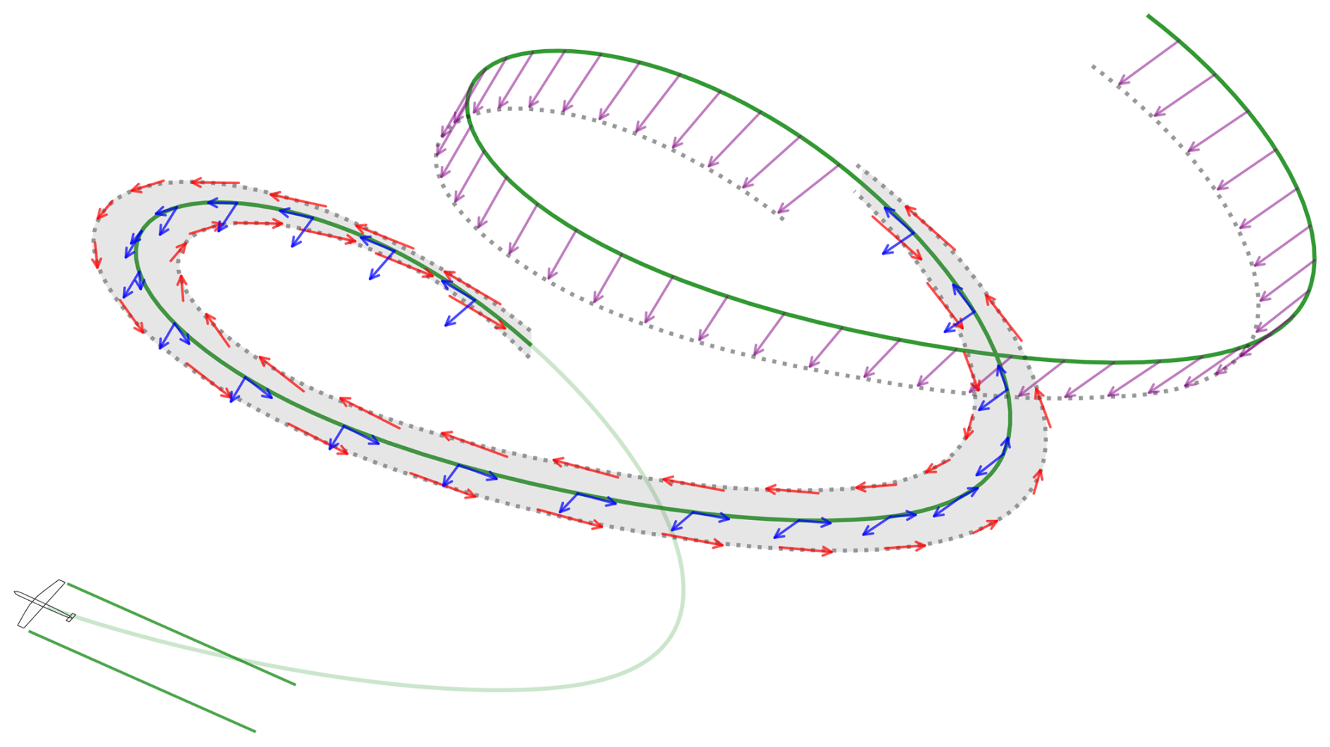
Figure 3 Illustration of the proposed hybrid rectangle–dipole model. The first half period of the trailing wake is modelled as a straight-flight wake. Then, a full period is modelled using the continuous vortex-loop model, and all remaining periods are modelled using the continuous dipole model.

We devise the hybrid model by splitting the integrals in Eq. (19) at the location τ=T_A for the self-induced velocity of each wing and at location τ=T_B for the velocity induced by the wake of the other wing. For wing i=1, this gives

$$\begin{array}{}\text{(28)}& \begin{array}{rl}{\mathit{u}}_{\mathrm{1}}^{\mathrm{f}}\left({\mathit{q}}_{\mathrm{1}}\right(t),\mathit{y}(t,\cdot \left)\right)& :=\underset{T}{\overset{T_{\mathrm{A}}}{\int }}{\mathit{u}}^{\prime }\left({\mathit{q}}_{\mathrm{1}}\right(t),{\mathit{y}}_{\mathrm{1}}(t,\mathit{\tau }\left)\right)\mathrm{d}\mathit{\tau }\\ & +\underset{T_{\mathrm{A}}}{\overset{\mathrm{\infty }}{\int }}{\mathit{u}}_{\mathrm{d}}^{\prime }\left({\mathit{q}}_{\mathrm{1}}\right(t),{\mathit{y}}_{\mathrm{1}}(t,\mathit{\tau }\left)\right)\mathrm{d}\mathit{\tau }\\ & +\underset{\mathrm{0}}{\overset{T_{\mathrm{B}}}{\int }}{\mathit{u}}^{\prime }\left({\mathit{q}}_{\mathrm{1}}\right(t),{\mathit{y}}_{\mathrm{2}}(t,\mathit{\tau }\left)\right)\mathrm{d}\mathit{\tau }\\ & +\underset{T_{\mathrm{B}}}{\overset{\mathrm{\infty }}{\int }}{\mathit{u}}_{\mathrm{d}}^{\prime }\left({\mathit{q}}_{\mathrm{1}}\right(t),{\mathit{y}}_{\mathrm{2}}(t,\mathit{\tau }\left)\right)\mathrm{d}\mathit{\tau },\end{array}\end{array}$$

where the induced velocity for wing i=2 is simply obtained by switching the wing indices for the variables q_i and y_i. For each wing, we ignore the self-induced velocity for the first time interval with length T.

In this formulation, we can retrieve the full vortex-loop model ($T_{\mathrm{A}}=T_{\mathrm{B}}=\mathrm{\infty }$), the full vortex dipole model ($T_{\mathrm{A}}=T,T_{\mathrm{B}}=\mathrm{0}$), or any variant in between.

4 Continuous wake model validation

To validate the new continuous wake formulation, we compare the model with the higher-fidelity, free-vortex software tool DUST (Tugnoli et al., 2021), an open-source, mid-fidelity aerodynamic solver specifically designed for analysing complex and non-conventional aircraft configurations. The software features a lifting-line method to compute the aerodynamic loads, coupled to a highly resolved simulation of the wake using a vortex particle method that allows it to capture the complex vortex-to-vortex interactions that are largely ignored in the proposed optimization model.

4.1 Wing geometry and wake simulation in DUST

Two near-elliptic wings are generated using a parametric mesh with 40 discrete spanwise sections of the NACA 4421 airfoil. The discretization introduces deviations from an ideal elliptical planform, leading to reduced aerodynamic efficiency. To account for this, a span efficiency factor e is incorporated into the induced-drag model (Eq. 14):

$$\begin{array}{}\text{(29)}& C_{\mathrm{D},i}:=C_{\mathrm{D},\mathrm{0}}+{\displaystyle \frac{C_{\mathrm{L},i}^{\mathrm{2}}}{\mathit{\pi }\mathrm{AR}e}},\end{array}$$

and the corresponding trailing vortex strength in Eq. (22) is scaled accordingly:

$$\begin{array}{}\text{(30)}& {\mathrm{\Gamma }}_i(t,\mathrm{0}):={\displaystyle \frac{\mathrm{2}b}{\mathit{\pi }\mathrm{AR}e}}{C}_{\mathrm{L},i}\left(t\right)\parallel {\mathit{u}}_{\mathrm{a},i}\left(t\right)\parallel .\end{array}$$

The efficiency factor, e≈0.75, is identified from a series of straight-flight DUST simulations across varying angles of attack. Inflow speeds are chosen to match the apparent wind conditions of the validation flight trajectory, ensuring consistency in Reynolds number. The factor e is then obtained by fitting Eq. (29) to the simulated drag polar.

To simulate the wake in DUST, we must prescribe a kinematic flight trajectory for the wings. To obtain a representative trajectory, we feed into DUST the optimal periodic wing position trajectories and orientations obtained by solving the optimization problem defined by Eq. (59) from Sect. 5. The rationale behind the dual-kite set-up is to generate an extremely high-load scenario with a small convection distance between the wings and the trailing vorticity structure. This constitutes a worst-case test for the ability of the vortex-loop model to accurately represent the induced velocity close to the wake structure. Lower-load scenarios (e.g. with a medium-scale single-wing system) are expected to be less demanding and to be representable with at least comparable, if not improved, accuracy.

One remaining problem is that the angle of attack is not explicitly modelled in the optimal orientation trajectory, since the optimization model assumes direct lift coefficient control. Therefore, in a preprocessing step, we apply a pitch correction to impose the angle of attack that would produce the same lift coefficient under the same conditions (including the induction effects predicted by the wake model), using the simulated 3D lift polar.

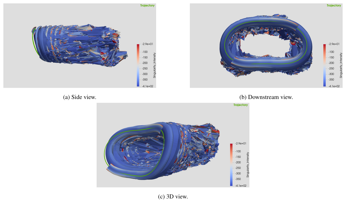
Figure 4 DUST wake simulation result over 6.5 flight loops as visualized in Paraview. The flight trajectory is visualized in green.

The simulation is initialized in a vortex-free state, with vortex particles being shed during the simulation. We run the DUST simulation for 6.5 periods of the optimal state trajectory to allow for the wake build-up to reach a steady state. Figure 4 visualizes the simulation result, showing a distinct helicoidal wake structure in the first part of the wake, followed by an increasing break-up of this structure due to the vortex-to-vortex interactions. In postprocessing, we can retrieve the vortex particle trajectories, the induced velocity field at all time steps, and the aerodynamic loads obtained from the lifting-line approach. The toolchain to generate the necessary DUST input files as well as the input data and more detailed simulation settings (e.g. particle size) are made publicly available.

4.2 Wake convection comparison

To compare the DUST wake simulation with the proposed wake model, we evaluate the wake using the analytic solution defined by Eq. (18) and compute the induced velocities via Eq. (19) using a high-accuracy numerical integration scheme, running the integral up to 6.5 periods in the past. For the forcing term in Eq. (18), describing the wake convection, we consider three different convection velocity variants. For each variant, we obtain a different wake solution and a different time-dependent induced velocity field, which can be used to correct the aerodynamic loads obtained in the prescribed flight trajectory.

The first variant (“free”) assumes no vortex-to-vortex interaction at all and prescribes convection with the free-stream wind velocity:

$$\begin{array}{}\text{(31)}& {\mathit{u}}_{\mathrm{conv},i}\left(\mathit{y}\right(t-\mathit{\tau },\cdot \left)\right):={\mathit{u}}_{\mathrm{\infty }}.\end{array}$$

The second variant (“far”) assumes convection with reduced velocity due to far-wake induction at the time of shedding; i.e.

$$\begin{array}{}\text{(32)}& {\mathit{u}}_{\mathrm{conv},i}\left(\mathit{y}\right(t-\mathit{\tau },\cdot \left)\right):={\mathit{u}}_{\mathrm{\infty }}+{\mathit{u}}_i^{\mathrm{f}}\left({\mathit{q}}_{\mathrm{v},i}\right(t-\mathit{\tau },\mathrm{0}),\mathit{y}(t-\mathit{\tau },\mathrm{0}\left)\right).\end{array}$$

The third variant (“near”) assumes convection with reduced velocity due to “near-wake” self-induction, as proposed by Trevisi et al. (2023); i.e.

$$\begin{array}{}\text{(33)}& {\mathit{u}}_{\mathrm{conv},i}\left(\mathit{y}\right(t-\mathit{\tau },\cdot \left)\right):={\mathit{u}}_{\mathrm{\infty }}-{\displaystyle \frac{C_{\mathrm{L},i}\parallel {\mathit{u}}_{\mathrm{a},i}\parallel }{\mathit{\pi }\mathrm{AR}e}}{\mathit{e}}_x.\end{array}$$

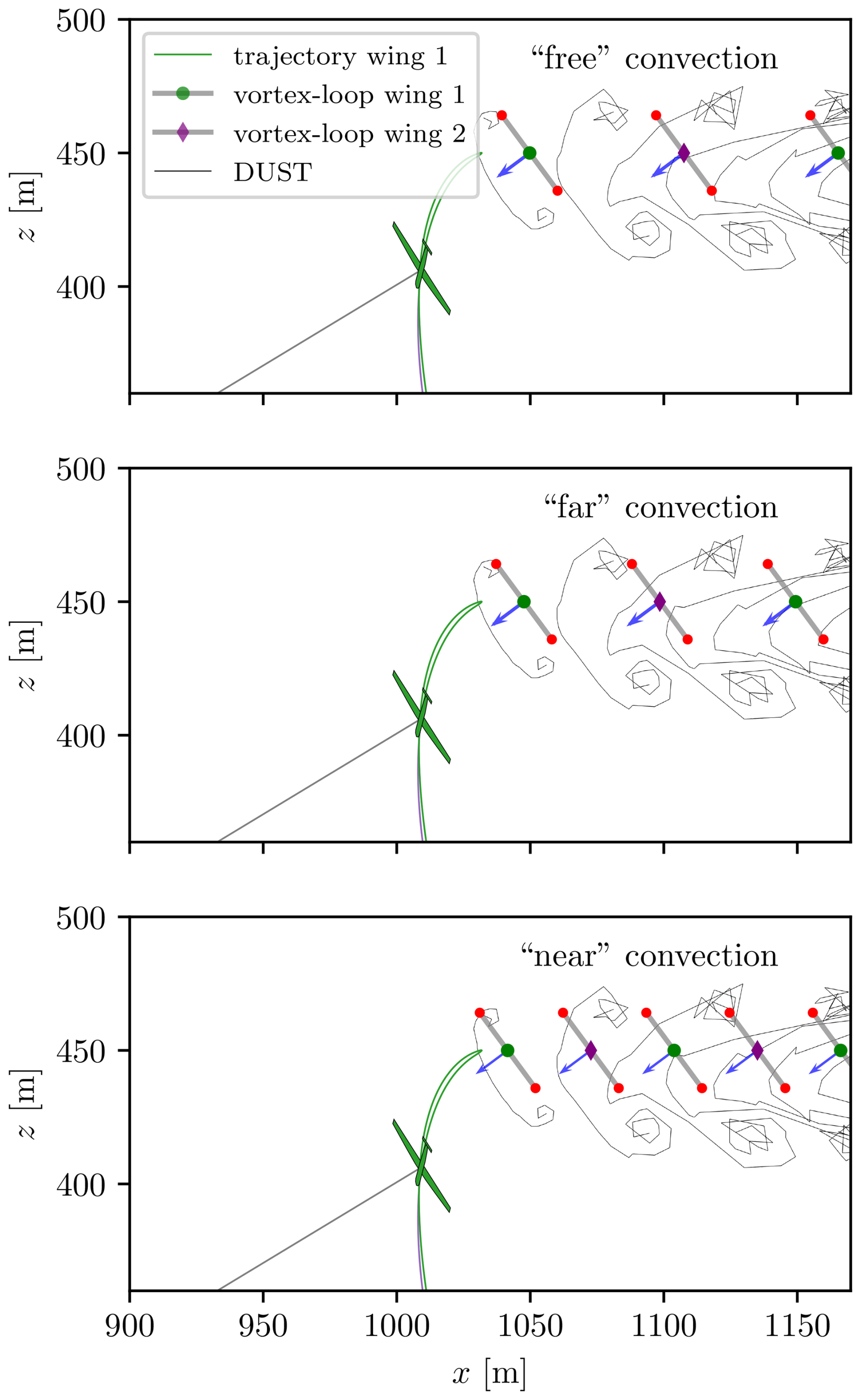
Figure 5 Comparison of snapshots of the vortex-loop wake position and orientation for the three convection velocity variants plotted against the DUST simulation, for fully developed wakes of 6.5 periods and at the intersections with the xz plane. The snapshots focus on the top part of the wake. The trajectory of wing 1 is included, as well as the position and orientation of wing 1 at the time of the snapshot. The blue arrows represent the normal unit vectors e_n,i of the vortex loops. The red dots visualize the boundaries of the vortex loops which should coincide with the location of the rolled-up tip vortices.

Figure 5 shows the position in the xz plane of the DUST vortex particles for the upper part of the wake. We compare this result with the predicted vortex-loop wake trajectory and orientation as they cross this plane, for each of the three variants. Firstly, it is visible that in the first, most influential part of the wake, the wake orientation and the distance between the tip vortices match well with the DUST simulation, although the bottom DUST tip vortex is convected slightly downwards. Further downstream, the models start to diverge due to wake deformation and expansion.

We can now assess the convection velocity fit by comparing the locations of the tip vortices predicted by both models. The “free” variant strongly overestimates the convection velocity, as the consecutive DUST tip vortices pop up much sooner and closer to the wing trajectory. For the “near” variant, the opposite is true: it provides a strong underestimation. The “far” variant provides the best fit, although some overestimation remains. In the remainder of this work, we apply the latter variant and delegate further improvements to future work.

4.3 Comparison of the induced velocity at the wing and the aerodynamic loads

For the purpose of optimal control, we are primarily interested in the induced velocity evaluated at the wing position and its effect on the aerodynamic loads. However, the DUST model does not differentiate between the induced velocity by the “far”-wake structure and the local circulation around the wing that produces lift, as we do in the optimization model. Thus, to eliminate the local circulation effect around the wing, we probe the wind field by means of an imaginary pitot tube of length l_p=0.9b pointing forward in the chord direction. For the vortex-loop model, we evaluate the induced velocity at the same location:

$$\begin{array}{}\text{(34)}& {\widehat{\mathit{u}}}_i^{\mathrm{f}}\left(t\right):={\mathit{u}}_i^{\mathrm{f}}\left({\mathit{q}}_i\right(t)+l_{\mathrm{p}}{\mathit{e}}_{\mathrm{c},i}(t),\mathit{y}(t,\cdot \left)\right),\end{array}$$

with e_c,i being the pitch-corrected chordwise body frame vector.

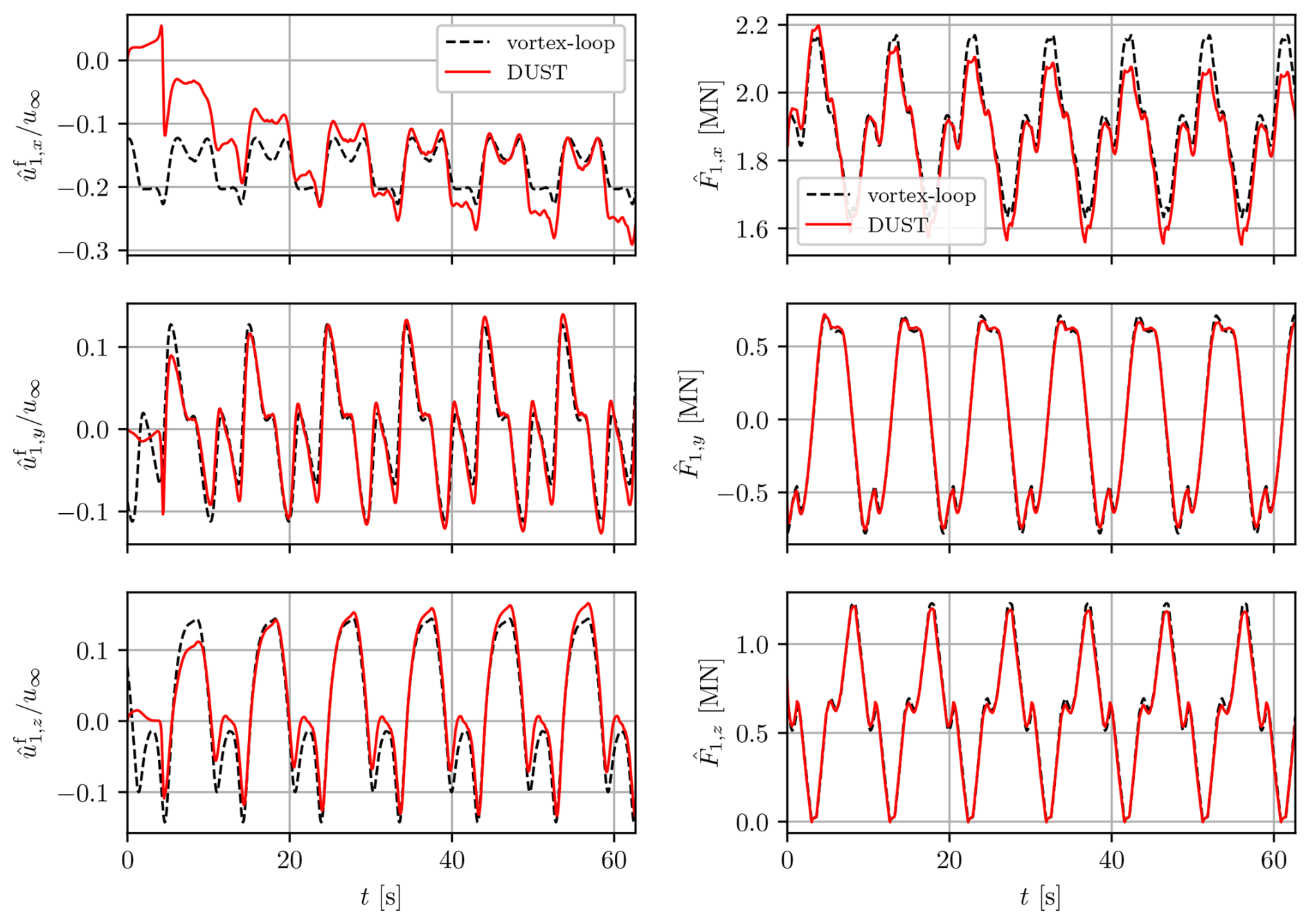
Figure 6 Comparison of the induced velocity (left) and aerodynamic force (right) components corresponding to the continuous vortex-loop and DUST simulations. Note that the vortex-loop profiles are periodic and correspond to a developed wake of 6.5 periods, whereas the DUST simulation starts with no wake history, and thus we can observe the wake build-up.

Figure 6 (left) shows the component-wise comparison of the measured induced velocity, normalized with the free-stream wind speed. For the first half rotation, the DUST induced velocity is almost zero, as the wake has not developed yet. After that, the magnitude of the induced velocity increases rotation after rotation as the wake builds up until it reaches a steady state. When comparing the induced velocities at the end of the DUST simulation with those from the periodic vortex-loop simulation, we see very good agreement between the y and z components. Also for the x component, the vortex-loop model captures the unsteady nature of the wake very well. However, due to the overestimation in convection velocity, the vortex-loop model underestimates the induced velocity by up to 25 % in the dominant x direction.

Figure 6 (right) shows the effect of this mismatch on the different components of the aerodynamic loads ${\widehat{\mathit{F}}}_i:={\mathit{F}}_{\mathrm{L},i}+{\mathit{F}}_{\mathrm{D},i}$. Again, we have very good agreement in the y and z directions. In the x direction, the induced velocity mismatch leads to an overestimation of the angle of attack and consequently an overestimation of the loads up to 5 %.

In summary, the vortex-loop model provides a strong match with the DUST benchmark. The y and z components of the induced velocities are captured with high accuracy. In the dominant x direction there is a moderate mismatch, mainly resulting from the limitations of the convection model. Nevertheless, it is important to note that the model reproduces the unsteady and non-axisymmetric nature of the wake, which conventional approaches fail to represent, very well.

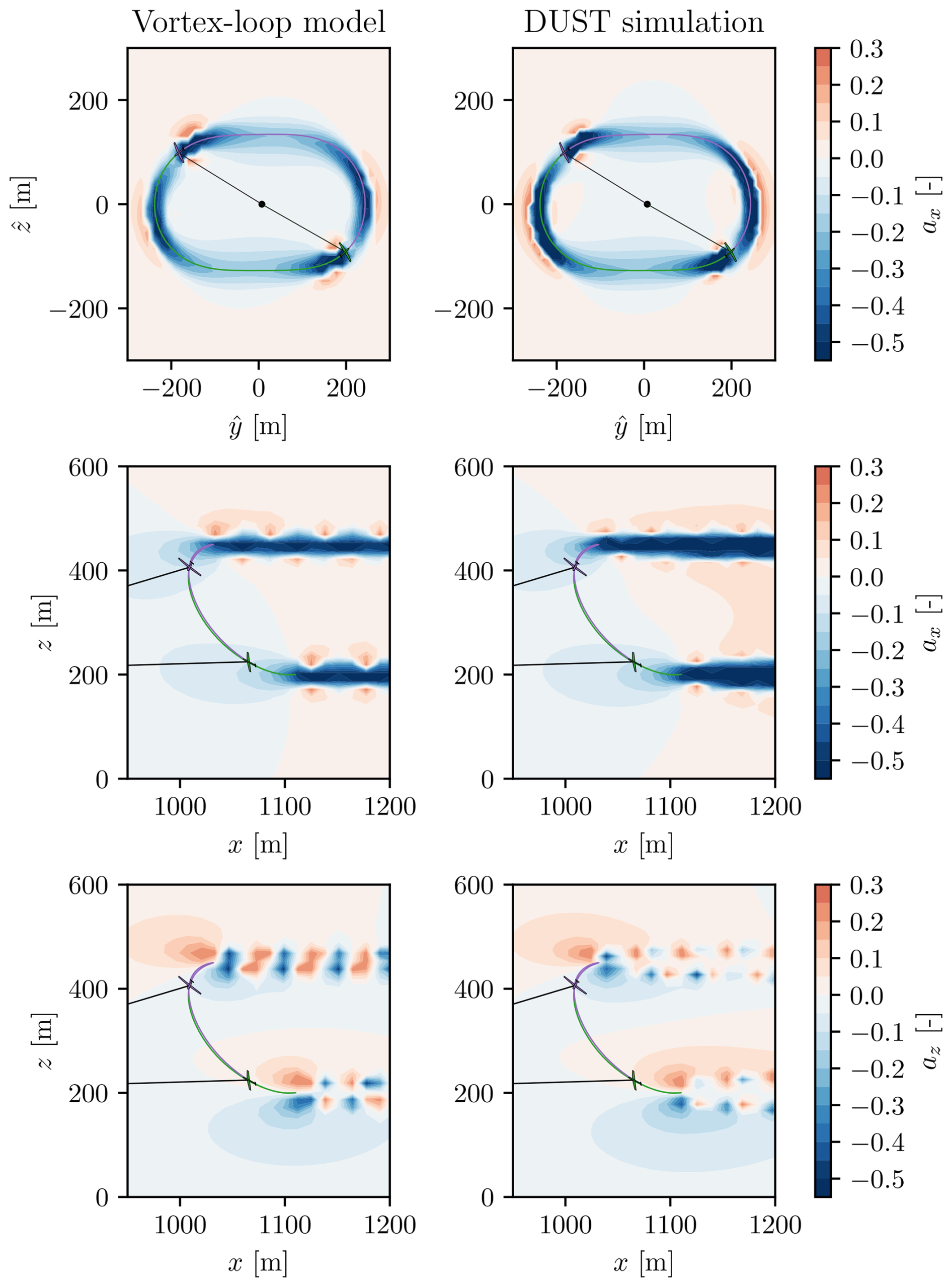
Figure 7 Snapshot of the axial induction factor fields ($a_x:=\frac{u_x^{\mathrm{f}}(\mathit{q},\mathit{y}(t,\cdot \left)\right)}{u_{\mathrm{\infty },x}}$) in the $\widehat{y}\widehat{z}$ plane perpendicular to the average main tether direction, located at the average wing position (top row), in the plane defined by y=0 (middle row) and the vertical induction factor $a_z:=\frac{u_z^{\mathrm{f}}(\mathit{q},\mathit{y}(t,\cdot \left)\right)}{u_{\mathrm{\infty },x}}$) in the plane defined by y=0. Note that we include the “near-wake” part of the vortex x-loop induction; i.e. the first integral in Eq. (19) starts at τ=0. The wing trajectories are included in green (wing 1) and purple (wing 2). The wings are drawn at their position and with their orientation at the moment of the snapshot.

4.4 Comparison of the induced velocity field in the neighbourhood of the wing

For optimization purposes, it is important to have a good model for the induced velocity evaluated not only at the wing position, but also in its surrounding neighbourhood. Therefore, we also compare the induced velocity field of the vortex-loop model with that of DUST in the region around the optimal trajectory. Figure 7 (top row) shows a snapshot of the wake at the same time point t^′ as in Fig. 5. It shows the induction factor a_x in the x direction in a plane perpendicular to the average main tether direction, located at the average wings' position. The induction factor is computed taking into account the contribution of the entire wake. Figures 7 (middle row) and 7 (bottom row) plot the induction factor in the x and z directions. In accordance with the findings in the previous section, we can discern a slight overall underestimation of the induced velocities in front of the wake. Nevertheless, the qualitative fit is very good in all directions.

5 Efficient problem formulation

After the validation of the proposed wake model in the previous section, the goal of this section is to use this model in optimal control problem (OCP) formulations and outline the transcription and approximation steps taken to arrive at an efficient implementation. Therefore we first formulate the envisaged PDE-based optimal control problem in continuous time. Then we propose a wake discretization strategy using auxiliary wake states. This approach transcribes the PDE optimization problem into a standard continuous-time OCP with state jump constraints for the wake states. Finally, we introduce further simplifications to render the final OCP numerically tractable.

5.1 PDE optimal control problem

For all types of crosswind kite systems, the challenge is to compute periodic flight orbits that maximize a certain averaged performance index. In the AWE case, the performance index is typically the power output. For the atmospheric airborne actuator case, as well as for the ship-towing case, the tether-pulling force is to be maximized. For the airborne actuator case, this metric is used as a proxy for the amount of momentum that it can redirect into the wind farm:

$$\begin{array}{}\text{(35)}& l\left(\mathit{x}\right(t),\mathit{u}(t),\mathit{z}(t),\mathit{\theta }):=-F_{\mathrm{t}}\left(t\right):=-{\mathit{\lambda }}_{\mathrm{0}}\left(t\right)l_{\mathrm{t}}\end{array}$$

while satisfying the following constraints:

$$\begin{array}{}\text{(36)}& \mathit{h}\left(\mathit{x}\right(t),\mathit{u}(t),\mathit{z}(t),\mathit{\theta }):=\left[\begin{array}{c}\mathit{\pi }{d}_{\mathrm{t}}^{\mathrm{2}}{\mathit{\sigma }}_{\max }-\mathrm{4}{F}_{\mathrm{t}}\left(t\right)\\ (\mathrm{2.2}b{)}^{\mathrm{2}}-({\mathit{q}}_{\mathrm{2}}-{\mathit{q}}_{\mathrm{1}}{)}^{\top }({\mathit{q}}_{\mathrm{2}}-{\mathit{q}}_{\mathrm{1}})\\ \mathit{\nu }-{\mathit{\nu }}_{\min }\\ {\mathit{\nu }}_{\max }-\mathit{\nu }\end{array}\right]\ge \mathrm{0},\end{array}$$

which impose a maximum tether stress constraint, an anticollision constraint, and the bounds on the variables $\mathit{\nu }:=(\mathit{x},\mathit{u},\mathit{z},\mathit{\theta },T)$.

Further, since the optimal state trajectory will be periodic, the wake state will be periodic in t as well. Therefore we can reformulate the wake transport equation as

$$\begin{array}{}\text{(37)}& {\displaystyle \frac{\mathrm{d}\mathit{y}}{\mathrm{d}t}}(t,\mathit{\tau })+{\displaystyle \frac{\mathrm{d}\mathit{y}}{\mathrm{d}\mathit{\tau }}}(t,\mathit{\tau })=\mathit{f}\left(\mathit{y}\right([t-\mathit{\tau }],\cdot \left)\right),\end{array}$$

with the modulo operator [t]:=t mod T so that the wake state only needs to be tracked for $t\in \left[\mathrm{0},T\right]$. Using this reformulation, we can formulate the following continuous and periodic PDE optimal control problem:

$$\begin{array}{l}\text{minimize}\\ \mathit{x}(\cdot ),\mathit{u}(\cdot ),\mathit{z}(\cdot )\\ \mathit{y}(\cdot ,\cdot ),\mathit{\theta },T\end{array}{\displaystyle \frac{\mathrm{1}}{T}}\underset{\mathrm{0}}{\overset{T}{\int }}l\left(\mathit{x}\right(t),\mathit{u}(t),\mathit{z}(t),\mathit{\theta })\mathrm{d}t$$

subject to

$$\begin{array}{}\text{(38)}& \begin{array}{rll}\mathit{F}\left(\mathit{x}\right(t),\dot{\mathit{x}}(t),\mathit{u}(t),\mathit{z}(t),\mathit{y}(t,\cdot ),\mathit{\theta })& =\mathrm{0}& t\in [\mathrm{0},T]\\ \mathit{h}\left(\mathit{x}\right(t),\mathit{u}(t),\mathit{z}(t),\mathit{\theta })& \ge \mathrm{0},& t\in [\mathrm{0},T]\\ {\displaystyle \frac{\mathrm{d}\mathit{y}}{\mathrm{d}t}}(t,\mathit{\tau })+{\displaystyle \frac{\mathrm{d}\mathit{y}}{\mathrm{d}\mathit{\tau }}}(t,\mathit{\tau })-\mathit{f}\left(\mathit{y}\right([t-\mathit{\tau }],\cdot \left)\right)& =\mathrm{0}& t\in [\mathrm{0},T]\\ & & \mathit{\tau }\in [\mathrm{0},\mathrm{\infty })\\ \mathit{y}(t,\mathrm{0})-\mathit{g}\left(\mathit{x}\right(t),\mathit{y}(t,\cdot \left)\right)& =\mathrm{0}& t\in [\mathrm{0},T]\\ \mathit{x}\left(\mathrm{0}\right)-\mathit{x}\left(T\right)& =\mathrm{0}.& \end{array}\end{array}$$

This problem is infinite-dimensional in both t and τ and numerically intractable. The first step is to transcribe the problem into a form that is only infinite-dimensional in t.

5.2 Wake transcription

We propose discretizing the wake on a uniform grid of M points in the τ space:

$$\begin{array}{}\text{(39)}& \mathrm{0}<{\mathit{\tau }}_{\mathrm{1}}<\mathrm{\dots }<{\mathit{\tau }}_j<\mathrm{\dots }<{\mathit{\tau }}_M<T,\end{array}$$

and introduce the periodic wake state on this grid

$$\begin{array}{}\text{(40)}& {\mathit{y}}^{\left(j\right)}\left(t\right)\approx \mathit{y}(t,t+{\mathit{\tau }}_j),\end{array}$$

which approximately tracks the evolution of points j in the wake, originating at a time $t=\left[-{\mathit{\tau }}_j\right]=T-{\mathit{\tau }}_j$, which are convected away as time progresses. We can derive that the derivative of this wake state should approximate the forcing term in Eq. (37):

$$\begin{array}{}\text{(41)}& {\dot{\mathit{y}}}^{\left(j\right)}\left(t\right)\approx \mathit{f}\left(\mathit{y}\right(\left[-{\mathit{\tau }}_j\right],\cdot \left)\right),\end{array}$$

and we model its origination as an impulsive event along its periodic trajectory:

$$\begin{array}{}\text{(42)}& {\mathit{y}}^{\left(j\right)}\left({\left[-{\mathit{\tau }}_j\right]}^{+}\right)\approx \mathit{g}\left(\mathit{x}\right({\left[-{\mathit{\tau }}_j\right]}^{-}),\mathit{y}({\left[-{\mathit{\tau }}_j\right]}^{-},\cdot \left)\right).\end{array}$$

Note how in Eq. (41) the individual derivatives each depend on the entire wake history, which is counterproductive as it produces cross-couplings over different time instances. To arrive at a more classical state equation, we propose extending the wake states with these derivatives and collecting both in one overall wake state:

$$\begin{array}{}\text{(43)}& \mathit{Y}\left(t\right):=\left[\begin{array}{c}{\mathit{y}}^{\left(\mathrm{1}\right)}\left(t\right)\\ {\dot{\mathit{y}}}^{\left(\mathrm{1}\right)}\left(t\right)\\ \mathrm{⋮}\\ {\mathit{y}}^{\left(M\right)}\left(t\right)\\ {\dot{\mathit{y}}}^{\left(M\right)}\left(t\right)\end{array}\right].\end{array}$$

The state equation is trivially given by (assuming rigid convection)

$$\begin{array}{}\text{(44)}& \dot{\mathit{Y}}\left(t\right)={\mathit{F}}_Y\left(\mathit{Y}\right(t\left)\right):=\left[\begin{array}{c}{\dot{\mathit{y}}}^{\left(\mathrm{1}\right)}\left(t\right)\\ \mathrm{0}\\ \mathrm{⋮}\\ {\dot{\mathit{y}}}^{\left(M\right)}\left(t\right)\\ \mathrm{0}\end{array}\right],\end{array}$$

and the impulse effect can be written as

$$\begin{array}{}\text{(45)}& \mathit{Y}\left({\left[-{\mathit{\tau }}_j\right]}^{+}\right)={\mathit{G}}_j\left(\mathit{x}\right({\left[-{\mathit{\tau }}_j\right]}^{-}),\mathit{Y}({\left[-{\mathit{\tau }}_j\right]}^{-}\left)\right),\end{array}$$

with the impulse function defined as

$$\begin{array}{}\text{(46)}& {\mathit{G}}_j\left(\mathit{x}\right(t),\mathit{Y}(t\left)\right):=\left[\begin{array}{c}{\mathit{y}}^{\left(j\right)}\left(t\right)-\stackrel{\mathrm{̃}}{\mathit{g}}\left(\mathit{x}\right(t),\mathit{Y}(t\left)\right)\\ {\dot{\mathit{y}}}^{\left(j\right)}\left(t\right)-\stackrel{\mathrm{̃}}{\mathit{f}}\left(\mathit{Y}\right(t\left)\right)\end{array}\right].\end{array}$$

Here, the functions $\stackrel{\mathrm{̃}}{\mathit{f}}$ and $\stackrel{\mathrm{̃}}{\mathit{g}}$ are defined by replacing the induced velocity expression in the functions f and g as follows:

$$\begin{array}{}\text{(47)}& {\mathit{u}}_{\mathrm{1}}^{\mathrm{f}}(q_{\mathrm{1}},y(t,\cdot \left)\right)\approx {\stackrel{\mathrm{̃}}{\mathit{u}}}_{\mathrm{1}}^{\mathrm{f}}({\mathit{q}}_{\mathrm{1}},\mathit{Y}(t\left)\right),\end{array}$$

where the function ${\stackrel{\mathrm{̃}}{\mathit{u}}}_{\mathrm{1}}^{\mathrm{f}}$ is obtained via a numerical integration scheme based on the discretized wake state Y(t) (see below).

To simplify notation, we further only consider the hybrid model where each wing experiences its own induction through the dipole model only (T_A=T) and the induction caused by the other wing's wake only for one full rotation with the vortex-loop model (T_B=2T). As discussed later in Sect. 6, this model choice is sufficiently accurate compared to the full vortex-loop model. Nevertheless, the following developments can be worked out for all different hybrid variants as well.

The integrals in Eq. (28) extend over an infinite horizon in the τ domain, whereas the wake state Y(t) retains only a single period T of past history. However, using the analytic wake solution formula (Eq. 18) and exploiting the wake periodicity, we can look further in the past by introducing (e.g. for a wing “i”, as seen by wing “1”) a finite number N_d of “duplicate” wake states ${\mathit{y}}_{\mathrm{1}i,d}^{\left(j\right)}\left(t\right)$, based on the tracked wake states ${\mathit{y}}_i^{\left(j\right)}\left(t\right)$, which are convected downwind for d periods of duration T:

$$\begin{array}{}\text{(48)}& {\mathit{y}}_{\mathrm{1}i,d}^{\left(j\right)}\left(t\right):={\mathit{y}}_i^{\left(j\right)}\left(t\right)+(d+p_{\mathrm{1}i}^{\mathrm{n}}(t,{\mathit{\tau }}_j\left)\right)T{\dot{\mathit{y}}}_i^{\left(j\right)}\left(t\right).\end{array}$$

Note that we also introduced the “near-wake parameter” $p_{\mathrm{1}i}^{\mathrm{n}}(t,{\mathit{\tau }}_j)$, which ensures that we only consider the duplicates of those wake states that are in the near-wake region at the current time point t. Formally, this parameter is defined as (for $i\in \mathit{\{}\mathrm{1},\mathrm{2}\mathit{\}}$):

$$\begin{array}{}\text{(49)}& p_{ii}^{\mathrm{n}}(t,{\mathit{\tau }}_j):=\left\{\begin{array}{ll}\mathrm{1}& \mathrm{if}t\ge \left[-{\mathit{\tau }}_j\right],\\ \mathrm{0}& \mathrm{if}t<\left[-{\mathit{\tau }}_j\right],\end{array}\right.\end{array}$$

and

$$\begin{array}{}\text{(50)}& p_{\mathrm{12}}^{\mathrm{n}}(t,{\mathit{\tau }}_j):=\left\{\begin{array}{ll}\mathrm{0}& \mathrm{if}t\ge \left[-{\mathit{\tau }}_j\right],\\ \mathrm{1}& \mathrm{if}t<\left[-{\mathit{\tau }}_j\right],\end{array}\right.\end{array}$$

and $p_{\mathrm{21}}^{\mathrm{n}}=p_{\mathrm{12}}^{\mathrm{n}}$.

Based on the introduced duplicate wake states, the induced velocity for wing 1, using the hybrid model, can be computed numerically as follows using the midpoint integration rule:

$$\begin{array}{}\text{(51)}& \begin{array}{rl}{\stackrel{\mathrm{̃}}{\mathit{u}}}_{\mathrm{1}}^{\mathrm{f}}\left({\mathit{q}}_{\mathrm{1}}\right(t),\mathit{Y}(t\left)\right)& :=\sum _{i=\mathrm{1}}^{\mathrm{2}}\left(\sum _{d=\mathrm{1}}^{N_{\mathrm{d}}}\sum _{j=\mathrm{1}}^M{\mathit{u}}_{\mathrm{d}}^{\prime }\left({\mathit{q}}_{\mathrm{1}}\right(t\left)\right),{\mathit{y}}_{\mathrm{1}i,d}^{\left(j\right)}\left(t\right)\right)\mathrm{\Delta }\mathit{\tau }\\ & +\sum _{j=\mathrm{1}}^M{\mathit{u}}^{\prime }\left({\mathit{q}}_{\mathrm{1}}\right(t\left)\right),{\mathit{y}}_{\mathrm{1}i,\mathrm{0}}^{\left(j\right)}\left(t\right))\mathrm{\Delta }\mathit{\tau }.\end{array}\end{array}$$

The induced velocity ${\stackrel{\mathrm{̃}}{\mathit{u}}}_{\mathrm{2}}^{\mathrm{f}}\left({\mathit{q}}_{\mathrm{2}}\right(t),\mathit{Y}(t\left)\right)$ for wing 2 is simply obtained by a change of index.

5.3 Window of influence

At every time instance t, the induced velocities defined by Eq. (51) depend on the entire wake state Y(t). This results in a dense sensitivity structure for the dynamics, which ultimately leads to a high memory usage, and more time spent in the linear solver backend of the optimization solver. Experience showed that it is crucial to exploit the fact that the influence of each wake element at any given time depends on how close it is to the position of the wing at that time. Therefore, the contribution of more remote elements can be neglected at a low loss of accuracy. We implement this by assigning a moving window of influence to each wing.

To this end, we divide the time grid in N_w equidistant intervals

$$\begin{array}{}\text{(52)}& \mathrm{0}=t_{\mathrm{0}}<\mathrm{\dots }<t_k<\mathrm{\dots }<t_N=T,\end{array}$$

and as the wing passes through each interval, we only take into account the wake segments that originate from that particular interval and the neighbouring N_f intervals, as illustrated by Fig. 8.

Figure 8 Illustration of the proposed fixed window of influence for a dual-kite system with a number of intervals N_w=16, number of discrete vortex elements M=32, number of duplicates N_d=1, and number of neighbouring elements taken into account N_f=1 by the window of influence.

At a given time point t, we determine the current interval k as

$$\begin{array}{}\text{(53)}& k:=⌊{\displaystyle \frac{Nt}{T}}⌋,\end{array}$$

and the window that is taken into account in interval k is defined by the boundaries

$$\begin{array}{}\text{(54)}& {\displaystyle }{\underset{\mathrm{¯}}{T}}_{\mathrm{f},k}& {\displaystyle }:=t_k-N_{\mathrm{f}}{\displaystyle \frac{T}{N}},\text{(55)}& {\displaystyle }{\overline{T}}_{\mathrm{f},k}& {\displaystyle }:=t_{k+\mathrm{1}}+N_{\mathrm{f}}{\displaystyle \frac{T}{N}}.\end{array}$$

We then introduce the “far-wake parameters”

$$\begin{array}{}\text{(56)}& p_{ii}^{\mathrm{f}}(t,{\mathit{\tau }}_j):=\left\{\begin{array}{ll}\mathrm{1}& \mathrm{if}\left[-{\mathit{\tau }}_j\right]\in \left[{\underset{\mathrm{¯}}{T}}_{\mathrm{f},k},{\overline{T}}_{\mathrm{f},k}\right],\\ \mathrm{0}& \text{otherwise},\end{array}\right.\end{array}$$

and

$$\begin{array}{}\text{(57)}& p_{\mathrm{12}}^{\mathrm{f}}(t,{\mathit{\tau }}_j):=\left\{\begin{array}{ll}\mathrm{1}& \mathrm{if}\mathit{\{}-{\mathit{\tau }}_j,\mathrm{2}T-{\mathit{\tau }}_j\mathit{\}}\cap \left[{\underset{\mathrm{¯}}{T}}_{\mathrm{f},k},{\overline{T}}_{\mathrm{f},k}\right]\ne \mathrm{\varnothing }\\ \mathrm{0}& \text{otherwise},\end{array}\right.\end{array}$$

with $p_{\mathrm{21}}^{\mathrm{f}}=p_{\mathrm{12}}^{\mathrm{f}}$. This parameter is then used to switch the contribution of the individual wake elements on and off, e.g. for wing i=1,

$$\begin{array}{}\text{(58)}& \begin{array}{rl}{\stackrel{\mathrm{̃}}{\mathit{u}}}_{\mathrm{1}}^{\mathrm{f}}\left({\mathit{q}}_{\mathrm{1}}\right(t),\mathit{Y}(t\left)\right)& :=\sum _{i=\mathrm{1}}^{\mathrm{2}}\left(\sum _{d=\mathrm{1}}^{N_{\mathrm{d}}}\sum _{j=\mathrm{1}}^M{p}_{\mathrm{1}i}^{\mathrm{f}}(t,{\mathit{\tau }}_j){\mathit{u}}_{\mathrm{d}}^{\prime }\left({\mathit{q}}_{\mathrm{1}}\right(t\left)\right),{\mathit{y}}_{\mathrm{1}i,d}^{\left(j\right)}\left(t\right)\right)\mathrm{\Delta }\mathit{\tau }\\ & +\sum _{j=\mathrm{1}}^M{p}_{\mathrm{1}i}^{\mathrm{f}}(t,{\mathit{\tau }}_j){\mathit{u}}^{\prime }\left({\mathit{q}}_{\mathrm{1}}\right(t\left)\right),{\mathit{y}}_{\mathrm{1}i,\mathrm{0}}^{\left(j\right)}\left(t\right))\mathrm{\Delta }\mathit{\tau }.\end{array}\end{array}$$

The parameter N_f can then be tuned in numerical experiments to achieve the best trade-off between accuracy and computation time.

5.4 Continuous-time OCP implementation

By transcribing the wake model as detailed above, we can reformulate the PDE optimal control problem from Eq. (38) into the more standard continuous-time formulation

$$\begin{array}{l}\text{minimize}\\ \mathit{x}(\cdot ),\mathit{u}(\cdot ),\mathit{z}(\cdot )\\ \mathit{Y}(\cdot ),\mathit{\theta },T\end{array}{\displaystyle \frac{\mathrm{1}}{T}}\underset{\mathrm{0}}{\overset{T}{\int }}l\left(\mathit{x}\right(t),\mathit{u}(t),\mathit{z}(t),\mathit{\theta })\mathrm{d}t$$

subject to

$$\begin{array}{}\text{(59)}& \begin{array}{rll}\stackrel{\mathrm{̃}}{\mathit{F}}\left(\mathit{x}\right(t),\dot{\mathit{x}}(t),\mathit{u}(t),\mathit{z}(t),\mathit{Y}(t),\mathit{\theta })& =\mathrm{0}& t\in [\mathrm{0},T]\\ \mathit{h}\left(\mathit{x}\right(t),\mathit{u}(t),\mathit{z}(t),\mathit{\theta })& \ge \mathrm{0},& t\in [\mathrm{0},T]\\ \dot{\mathit{Y}}\left(t\right)-{\mathit{F}}_Y\left(\mathit{Y}\right(t\left)\right)& =\mathrm{0},& t\in [\mathrm{0},T]\\ \mathit{Y}\left({\left[{\mathit{\tau }}_j\right]}^{+}\right)-{\mathit{G}}_j\left(x\right(\left({\left[{\mathit{\tau }}_j\right]}^{-}\right),\mathit{Y}\left({\left[{\mathit{\tau }}_j\right]}^{-}\right))& =\mathrm{0},& j\in {\mathbb{I}}_{\mathrm{1}}^M\\ \mathit{x}\left(\mathrm{0}\right)-\mathit{x}\left(T\right)& =\mathrm{0}& \\ \mathit{Y}\left(\mathrm{0}\right)-\mathit{Y}\left(T\right)& =\mathrm{0},& \end{array}\end{array}$$

where the dynamics $\stackrel{\mathrm{̃}}{\mathit{F}}$ are obtained by inserting the induced velocity expression from Eq. (58) into the dynamics F.

Because the system under consideration is not reeling, a solution consisting of a single periodic flight loop is of practical interest. Moreover, specifically for this dual-kite case, we can consider the relevant solution where both wings fly identical trajectories, phase shifted by half a period. In this case, while one wing flies, e.g. the downstroke part, the other one simultaneously flies the upstroke. After half a period, the roles are reversed, and the first wing flies the identical upstroke and the other one the identical downstroke. To avoid simulating the same upstroke and downstroke twice, we can instead integrate the dynamics over only half an orbit, and instead of enforcing periodicity on the wing states, we can implement the “role reversal” by matching the end state of each wing to the initial state of the other, as proposed by Zanon et al. (2013):

$$\begin{array}{}\text{(60)}& \left[\begin{array}{c}{\mathit{x}}_{\mathrm{1}}\left(T\right)-{\mathit{x}}_{\mathrm{2}}\left(\mathrm{0}\right)\\ {\mathit{x}}_{\mathrm{2}}\left(T\right)-{\mathit{x}}_{\mathrm{1}}\left(\mathrm{0}\right)\end{array}\right],\end{array}$$

with ${\mathit{x}}_i:=({\mathit{q}}_i,{\dot{\mathit{q}}}_i,C_{\mathrm{L},i},{\mathit{\psi }}_i)$, for $i\in \mathit{\{}\mathrm{1},\mathrm{2}\mathit{\}}$. As a consequence, the variables N, N_w, and M can be reduced by a factor of 2 while still simulating the full flight loop and wake with identical accuracy. Only the number of duplicates should be doubled to retain the same wake history. The time variable T automatically becomes the desired half-rotation near-wake cut-off time period.

We then transcribe this problem into a nonlinear program (NLP) using a direct collocation approach. The OCP is discretized using N=8 collocation intervals. Each interval consists of four RadauIIa collocation points, and the transcription includes a time transformation approach to deal with the variable time grid, as detailed by De Schutter et al. (2023b). Additionally, the computational performance benefits from additional lifting of the induced velocities as algebraic variables to reduce nonlinearity and symbolic complexity. We implemented this problem in the open-source framework AWEbox (De Schutter et al., 2023b), which relies on the symbolic framework CasADi (Andersson et al., 2019) for automatic differentiation and the interface to the NLP solver IPOPT (Wächter and Biegler, 2006), using MA57 (HSL, 2011) as the linear solver backend. The problem is solved on an Intel Core i7 2.5 Ghz, 16 GB RAM.

6 Numerical example

In this section, we illustrate the proposed approach by means of a numerical case study where a highly resolved reference OCP with a wake model is solved, and the solution and computational expense are compared to those of a no-wake OCP. In a second step, we investigate the sensitivity of the OCP solution and its computational expense with respect to key transcription parameters.

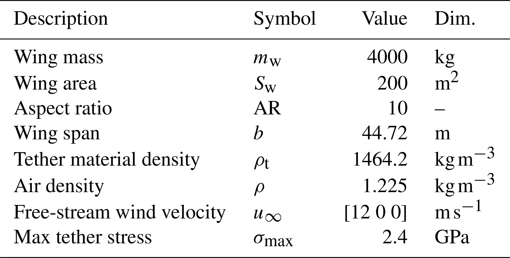
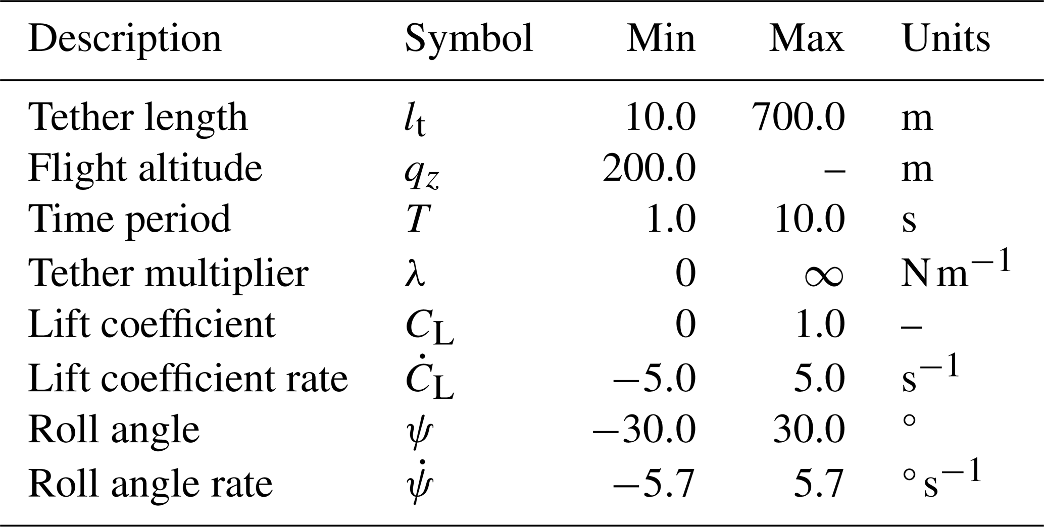
Table 1 Kite system model parameters used in the numerical example.

Table 2 System variable bounds.

6.1 OCP solution comparison

To illustrate the proposed approach, we solve the OCP from Eq. (59) for a dual-kite system using the numerical parameters provided by Table 1 and with the variable bounds ν_min and ν_max summarized in Table 2. As mentioned in Sect. 4, the dual-kite set-up is chosen to generate an interesting scenario for the validation. The wing size is chosen to be in the large-scale range envisaged by e.g. Kruijff and Ruiterkamp (2018) to decrease the sensitivity of the solution to tether drag in favour of the induction effects. Other properties and bounds represent typical values from the AWE literature, e.g. for tether properties (Malz et al., 2019) and aerodynamic properties and mass scaling (Zanon et al., 2013). The induction effects are roughly invariant with respect to the chosen wind speed. However, since the wind speed is chosen relatively high (${\mathit{u}}_{\mathrm{\infty }}=\mathrm{12}\mathrm{m}{\mathrm{s}}^{-\mathrm{1}}\cdot {\mathit{e}}_x$), the effect of the wing mass on the dynamic trajectory is rather small in this example.

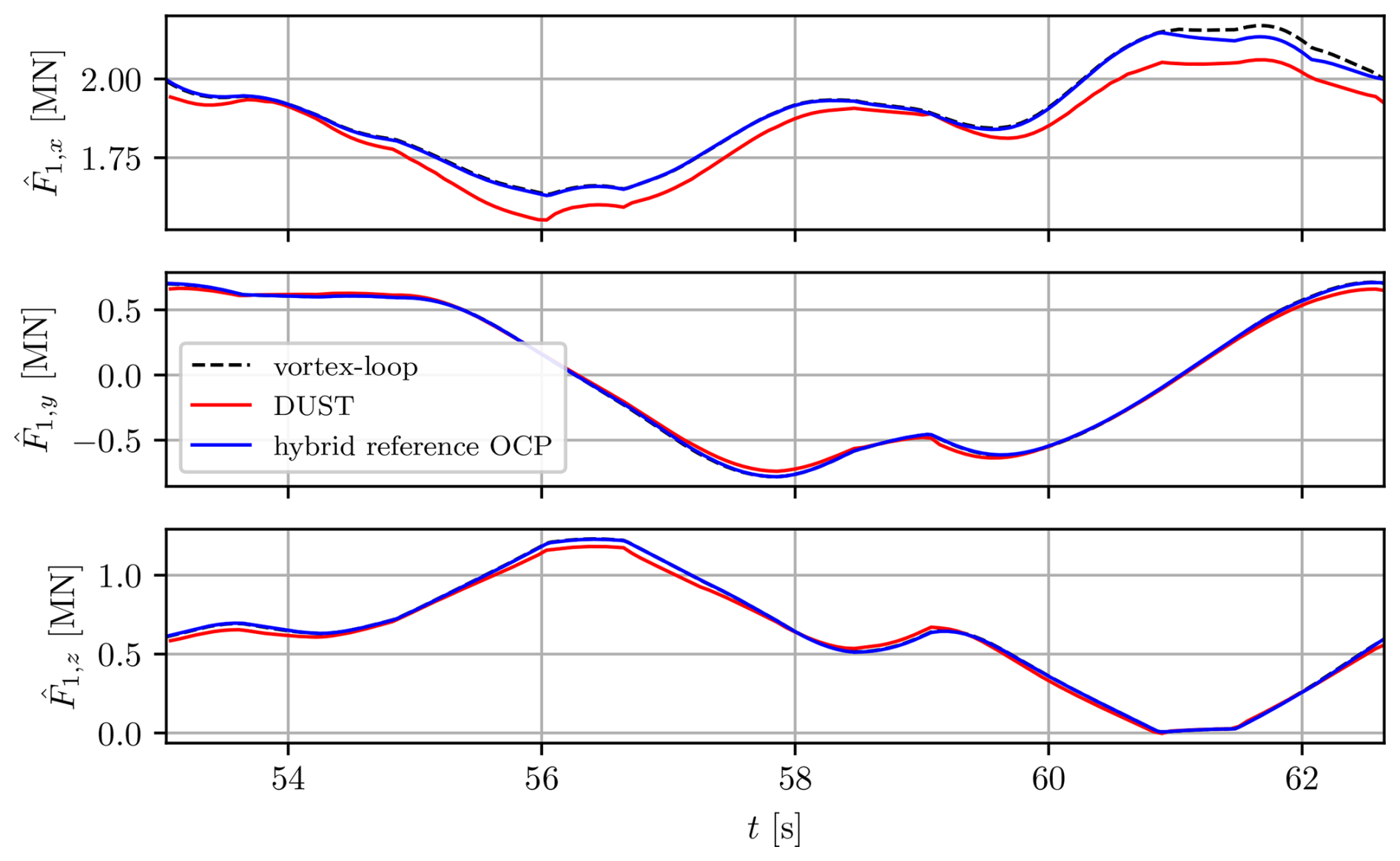
Figure 9 Comparison of the total aerodynamic forces obtained in the OCP with reference transcription of the hybrid model, with those obtained using the vortex-loop model and DUST simulation using the same boundary condition.

To generate a first reference solution, the wake discretization parameters are chosen so that a good fit with the post-ex analytic wake solution is achieved. Figure 9 shows the obtained total aerodynamic forces compared to the analytic vortex-loop and DUST simulations using the same boundary condition. The fit is very good, which validates not only the reference transcription, but also the hypothesis of the hybrid model: that only the initial part of the wake needs to be modelled with vortex loops but that the rest of it can be modelled accurately with vortex dipoles. Table 3 summarizes the chosen parameters. Note that these parameters are valid for the half-periodic formulation of the OCP.

Table 3 Wake discretization parameters used in the half-periodic OCP formulation.

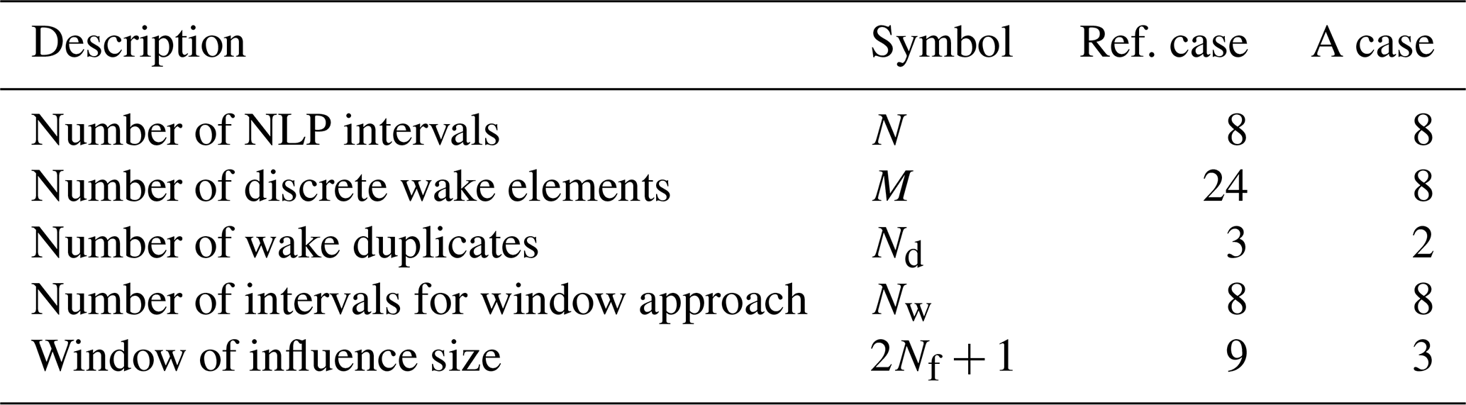
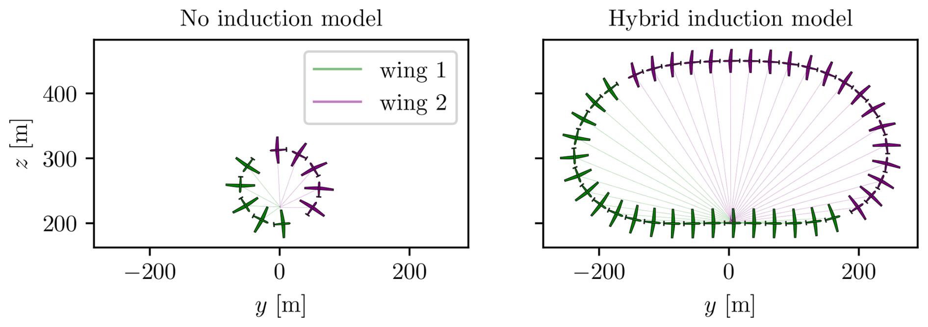
Figure 10 Optimal flight trajectories corresponding to the solution of the OCP from Eq. (59), where the induction is discarded (left) and where the hybrid induction model is used (right).

Figure 10 shows the resulting optimal flight trajectory in comparison to the case where no induction (NI) model is included. Note that the corresponding optimal wake state, induced velocities, and aerodynamic forces have already been discussed in Sect. 3 and shown in Figs. 4 to 7. Table 4 summarizes the main results of the optimization. The chosen induction model parameterization increases the computation time per iteration t_CPU by a factor of 16 compared to the NI case.

Table 4 Optimal solution indicators and computation time.

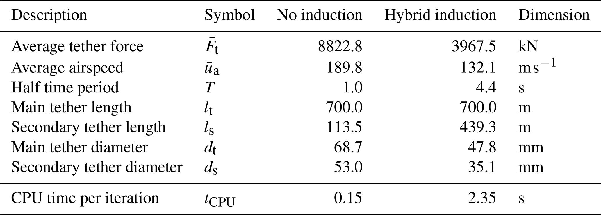
The optimizer increases the secondary tether lengths from 2.5 in the NI case to almost 10 wing spans. While this leads to higher tether drag losses, it allows the system to fly longer time periods T, which creates a larger convection distance between the system and its wake. Hence, the induction losses are reduced up to the point where the tether drag becomes dominant.

Also, because the available wind speed is reduced, the wings fly more slowly and experience a 30 % lower airspeed compared to the NI case, and they produce 55 % less average tether force. As a result, the tether diameters can be dimensioned smaller, which helps to dampen the effect of the increased tether drag. In conclusion, both the optimal design and the performance of the considered system are highly sensitive to the inclusion of induction effects.

We note that in this example, the resulting average airspeed of 190 m s⁻¹ in combination with the small turning radius leads to immense and practically infeasible centrifugal accelerations. A more realistic trajectory could be attained by lowering the design wind speed. Nevertheless, induction effects are roughly invariant with respect to the wind speed, and similar validation and design trade-off results are therefore expected for lower design wind speeds with lower flight speeds and therefore a more reasonable flight envelope.

Another improvement would be to add a mass-scaling law that takes into account the effect of the loading of the wing. In this very high loading case, this would lead to a significantly higher wing mass and therefore a different design trade-off possibly favouring even shorter tether lengths to minimize the upwards flight path length. However, in the dual-kite set-up considered here, where only one of the two wings flies upwards at a time, the effect of wing mass on the optimal trajectory is typically low (De Schutter, 2024), and we omit this extension for simplicity.

6.2 Discretization sensitivity

To assess the trade-off between computational effort and solution accuracy, we evaluate the impact of coarser wake parameterizations relative to the reference case. Each discretization parameter (M, N_d, and N_f) is independently reduced, while the others are held at their reference values. For each configuration, the optimal control problem is resolved, and the resulting computational cost and accuracy are compared against the reference solution. The error E is defined relative to the reference solution so as to capture both the accuracy of the cost and that of the optimal design:

$$\begin{array}{}\text{(61)}& E:=∥\left[\begin{array}{cc}\frac{{\overline{F}}_{\mathrm{t}}^{\ast }-{\overline{F}}_{\mathrm{t},\mathrm{ref}}^{\ast }}{{\overline{F}}_{\mathrm{t},\mathrm{ref}}^{\ast }}& \frac{{\mathit{\theta }}^{\ast }-{\mathit{\theta }}_{\mathrm{ref}}^{\ast }}{{\mathit{\theta }}_{\mathrm{ref}}^{\ast }}.\end{array}\right]∥\end{array}$$

Figure 11 shows the trade-off between computational cost and accuracy across the tested wake parameterizations, including the no-induction (NI) case.

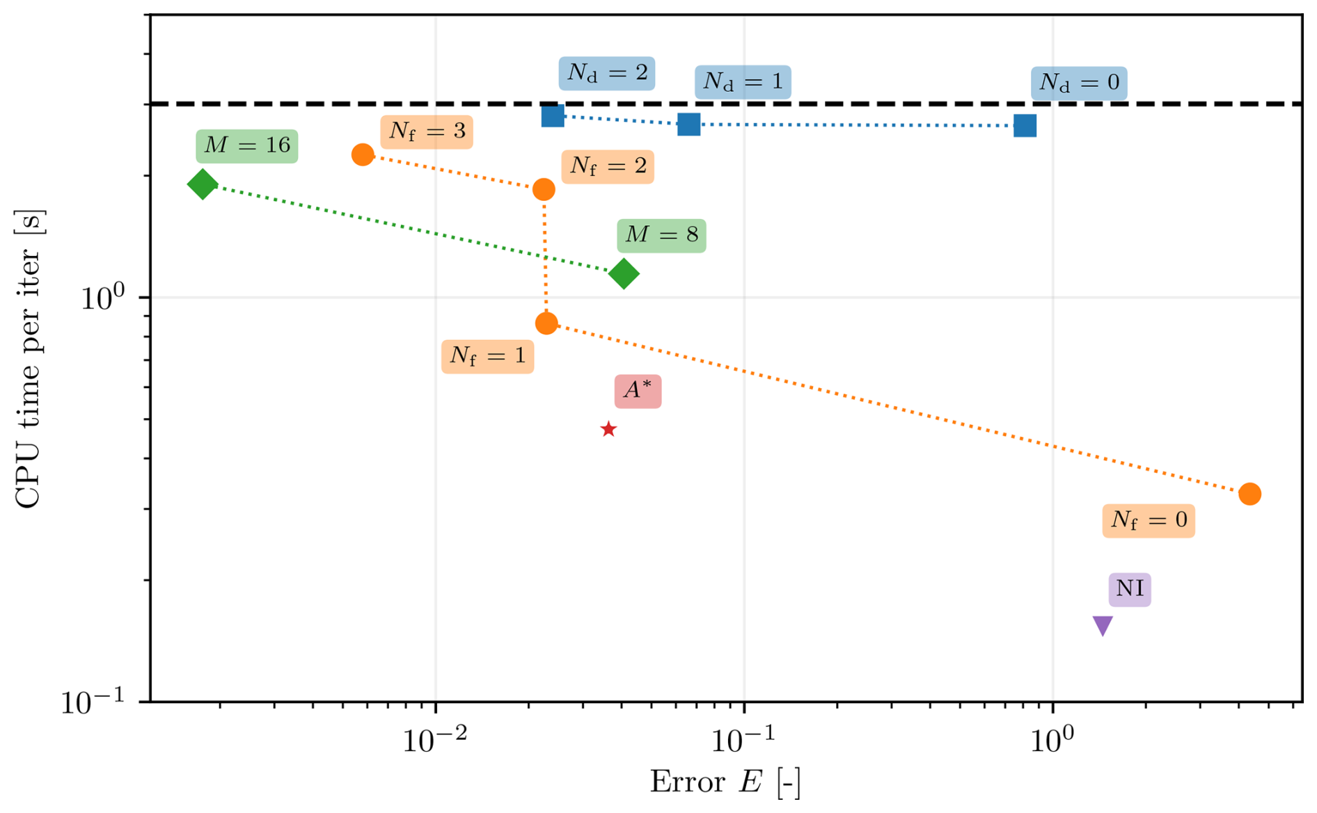
Figure 11 Comparison of CPU time vs. relative error E of different wake parameterizations compared to the reference parameterization (CPU time given by dashed black line).

As the number of wake duplicates is reduced (N_d↓), the solution accuracy is significantly affected. In particular, whether to include the first duplicate (N_d=1) or not has a large influence. The computation time, on the other hand, is hardly affected, as the duplicates do not change the NLP dimensions or sparsity pattern. This suggests that the number of duplicates should be carefully selected but that they can be added at little additional computational cost.

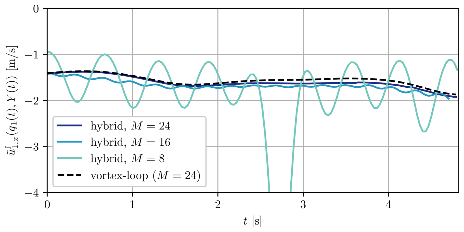
Figure 12 Time-resolved optimal far-wake induction profile (x component), evaluated at wing 1, for different numbers of wake elements M compared with the exact vortex-loop solution evaluated for M=24.

Reducing the window of influence size (N_f↓) significantly decreases computation time, as the resulting NLP becomes increasingly sparse. However, when the window is chosen too small (in this case, N_f=0), solution accuracy deteriorates, and a spurious trajectory is obtained that performs even worse than the no-induced-wake (NI) case. These observations justify the introduction of a finite window of influence and highlight N_f as a key discretization parameter governing the balance between numerical efficiency and model fidelity.

Finally, reducing the number of wake elements (M↓) leads to a moderate decrease in both computation time and solution accuracy, indicating that relatively coarse discretizations can still yield meaningful results. However, for small M, oscillations appear in the time-resolved profile of the induced velocity, as illustrated by Fig. 12. This behaviour arises from the dependence of the induced velocity on the wing position: when the wing passes directly over a wake element, the induced velocity reaches a peak and subsequently drops to a minimum halfway to the next element. Consequently, the integration error in Eq. (58) is position dependent and sensitive to the choice of collocation grid in the time-continuous OCP (Eq. 59). A potential remedy would be to implement a continuously moving window of influence that tracks the wing position, rather than the discrete interval-to-interval update scheme used here. While this would increase the computational complexity of the induced velocity evaluation, it could provide consistent integration accuracy, especially for small values of M. Such an extension is left for future work.

Figure 12 also shows the induced velocity from the analytic vortex-loop solution evaluated at the optimal solution for M=24. The induced velocity computed using the hybrid wake representation (comprising a single layer of vortex loops followed by dipole elements) shows good agreement with the one obtained from the full vortex-loop formulation, thereby justifying the use of dipoles for far-convected wake elements in this case. For applications involving larger convection distances, as are likely to occur for the case of single-kite AWE systems, the accuracy of the hybrid approximation is expected to improve further.

Based on the sensitivity analysis above, a new parameterization, denoted as “A”, is selected by choosing for each discretization parameter the lowest value that still yields a relative error E<5 %. This configuration represents a Pareto-efficient trade-off between computational cost and model fidelity among the tested cases. At point A, it also holds that E<5 %, while the average computation time per iteration is now only a factor of 3 more expensive than the NI case, which comes with a value of E=145 %. In conclusion, when very high accuracy is not required – such as during design exploration or when other modelling errors are of comparable magnitude – there exist parameterizations that provide approximate solutions of the PDE OCP from Eq. (38) with only a moderate increase in computation time compared to the NI case.

7 Conclusion and outlook

In this study, we introduced a novel continuous-time wake model for simulation and optimal control of crosswind kite systems. The new model is based on a hybrid combination of infinitesimal vortex-loop and dipole elements shed by the kites. Compared to existing vortex-based approaches, the model is capable of capturing the inherently unsteady and non-axisymmetric nature of how crosswind kite systems operate. Validation with the higher-fidelity free-vortex code DUST shows good agreement between the two simulations. One remaining point of mismatch is the wake convection velocity. In this study, three different heuristics for selecting the convection velocity were compared, and the best candidate was selected. However, this candidate overestimates the convection velocity, resulting in a remaining 5 % overestimation of the aerodynamic forces produced in the validation simulations. The model is also able to effectively capture the induced velocity field around the wing trajectory flown.

As a second contribution, we proposed a formulation that allows one to efficiently incorporate the new wake model into periodic optimal control problems. The formulation exploits the periodicity of the wake, and its efficacy particularly hinges on the introduction of a moving window of influence that only considers the part of the wake within a certain region around the flying wings' trajectory. Using an accurate reference parameterization of the wake model, the original (without wake) OCP cost is increased with a factor of 16. However, if we tolerate a loss of accuracy of 5 % compared to this accurate reference solution with a wake, we can achieve a modest slowdown of a factor of 3 compared to the original problem without a wake (which deviates from the reference solution with a wake with 145 %).

Apart from improving the model validity, future work should focus on improving the window of influence used in the OCP formulation. Ideally, this window would move continuously along with the wing and not just update as the wing passes from one interval to the next. Such an improvement would eliminate oscillations in the time-resolved induced velocity profile and result in consistent integration accuracy for the induced velocity expression.

In this work, we applied the new model to a dual-kite system and optimized its flight trajectory, consisting of one single loop, for maximum pulling force. Future work could focus on expanding to the following applications. First, we could extend the current example to a multi-loop scenario, where the wings fly multiple (possibly differing) loops within one period. While the wings cannot escape their own wake in the current one-loop example, in this new scenario, the wings would be able to adapt their trajectory during the subsequent loops to avoid the wake from the previous ones, thereby boosting performance. Second, future research could investigate the application to the single-wing airborne wind energy systems currently pursued by the AWE industry. While the flight trajectories of these systems are characterized by longer time periods as considered in the example of this paper, therefore necessitating a larger number of discrete wake elements, the wake model could still remain numerically tractable. Because of the long time period and long convection distance, it is likely that the initial vortex-loop part of the hybrid wake can be discarded in favour of the cheaper vortex dipole model, with less wake duplicates needed. This application would then enable one to compute wake-sensitive flight trajectories and provide an important stepping stone to realistically assess the achievable power density of these systems.

Appendix A: Induced velocity expression of a vortex-loop element with finite width

Consider a vortex-loop element as visualized in Fig. 2, characterized by the state $\mathit{y}:=({\mathit{q}}_{\mathrm{v}},\mathrm{\Gamma },{\mathit{e}}_{\mathrm{n}},{\mathit{e}}_{\mathrm{c}})$ and with a finite height $\frac{\mathit{\pi }}{\mathrm{4}}b$ and width Δs. The velocity induced by this element at a position q is given by applying the Biot–Savart law to all four finite vortex filaments of the vortex loop

$$\begin{array}{}\text{(A1)}& {\mathit{u}}_{\mathrm{vl}}(\mathit{q},\mathit{y},\mathrm{\Delta }s):=\sum _{i=\mathrm{1}}^{\mathrm{4}}{\mathit{u}}_{\mathrm{f},i},\end{array}$$

with

$$\begin{array}{}\text{(A2)}& {\displaystyle }{\mathit{u}}_{\mathrm{f},\mathrm{1}}& {\displaystyle }:={\mathit{u}}_{\mathrm{f},\mathrm{bs}}(\mathit{q},{\mathit{p}}_{\mathrm{1}},{\mathit{e}}_{\mathrm{b}},{\displaystyle \frac{\mathit{\pi }b}{\mathrm{4}}},\mathrm{\Gamma })\text{(A3)}& {\displaystyle }{\mathit{u}}_{\mathrm{f},\mathrm{2}}& {\displaystyle }:={\mathit{u}}_{\mathrm{f},\mathrm{bs}}(\mathit{q},{\mathit{p}}_{\mathrm{2}},{\mathit{e}}_{\mathrm{c}},\mathrm{\Delta }s,\mathrm{\Gamma })\text{(A4)}& {\displaystyle }{\mathit{u}}_{\mathrm{f},\mathrm{3}}& {\displaystyle }:={\mathit{u}}_{\mathrm{f},\mathrm{bs}}(\mathit{q},{\mathit{p}}_{\mathrm{3}},-{\mathit{e}}_{\mathrm{b}},{\displaystyle \frac{\mathit{\pi }b}{\mathrm{4}}},\mathrm{\Gamma })\text{(A5)}& {\displaystyle }{\mathit{u}}_{\mathrm{f},\mathrm{4}}& {\displaystyle }:={\mathit{u}}_{\mathrm{f},\mathrm{bs}}(\mathit{q},{\mathit{p}}_{\mathrm{4}},-{\mathit{e}}_{\mathrm{c}},\mathrm{\Delta }s,\mathrm{\Gamma }),\end{array}$$

where ${\mathit{e}}_{\mathrm{b}}:={\mathit{e}}_{\mathrm{n}}\times {\mathit{e}}_{\mathrm{c}}$ and where the four corners (anticlockwise) are

$$\begin{array}{}\text{(A6)}& {\displaystyle }{\mathit{p}}_{\mathrm{1}}& {\displaystyle }={\mathit{q}}_{\mathrm{v}}-{\displaystyle \frac{\mathrm{\Delta }s}{\mathrm{2}}}{\mathit{e}}_c-{\displaystyle \frac{\mathit{\pi }b}{\mathrm{8}}}{\mathit{e}}_b,\text{(A7)}& {\displaystyle }{\mathit{p}}_{\mathrm{2}}& {\displaystyle }={\mathit{q}}_{\mathrm{v}}-{\displaystyle \frac{\mathrm{\Delta }s}{\mathrm{2}}}{\mathit{e}}_c+{\displaystyle \frac{\mathit{\pi }b}{\mathrm{8}}}{\mathit{e}}_b,\text{(A8)}& {\displaystyle }{\mathit{p}}_{\mathrm{3}}& {\displaystyle }={\mathit{q}}_{\mathrm{v}}+{\displaystyle \frac{\mathrm{\Delta }s}{\mathrm{2}}}{\mathit{e}}_c+{\displaystyle \frac{\mathit{\pi }b}{\mathrm{8}}}{\mathit{e}}_b,\text{(A9)}& {\displaystyle }{\mathit{p}}_{\mathrm{4}}& {\displaystyle }={\mathit{q}}_{\mathrm{v}}+{\displaystyle \frac{\mathrm{\Delta }s}{\mathrm{2}}}{\mathit{e}}_c-{\displaystyle \frac{\mathit{\pi }b}{\mathrm{8}}}{\mathit{e}}_b,\end{array}$$

and with the Biot–Savart evaluation function

$$\begin{array}{}\text{(A10)}& \begin{array}{rl}{\mathit{u}}_{\mathrm{f},\mathrm{bs}}(\mathit{q},\mathit{p},\mathit{e},\mathrm{\ell },\mathrm{\Gamma })& :=-{\displaystyle \frac{\mathrm{\Gamma }}{\mathrm{4}\mathit{\pi }\Vert {\mathit{r}}_{\mathrm{1}}\times \mathit{e}{\Vert }^{\mathrm{2}}}}\left({\mathit{r}}_{\mathrm{1}}\times \mathit{e}\right)\\ & \cdot \left({\displaystyle \frac{\mathit{e}\cdot {\mathit{r}}_{\mathrm{1}}}{\Vert {\mathit{r}}_{\mathrm{1}}\Vert }}-{\displaystyle \frac{\mathit{e}\cdot {\mathit{r}}_{\mathrm{2}}}{\Vert {\mathit{r}}_{\mathrm{2}}\Vert }}\right),\end{array}\end{array}$$

where ${\mathit{r}}_{\mathrm{1}}:=\mathit{q}-\mathit{p}$ and ${\mathit{r}}_{\mathrm{2}}:={\mathit{r}}_{\mathrm{1}}-\mathrm{\ell }\mathit{e}$, with ℓ being the vortex filament length and e its unit direction vector. The linearization $\frac{\mathrm{d}{\mathit{u}}_{\mathrm{vl}}}{\mathrm{d}\mathrm{\Delta }s}$ used in Eq. (23) is finally obtained through algorithmic differentiation using CasADi.