Extreme wind speeds in tropical cyclones using parametric models

Tropical cyclones are among the most destructive natural disasters. Accurately estimating wind speeds during these extreme weather events remains a challenge but is essential for optimising the design of offshore structures, such as offshore wind turbines, which could be exposed to such phenomena. In this paper, a state-of-the-art parametric model fed with the best-track dataset is implemented to predict wind generated by tropical cyclones at hub height. The surface wind model accounts for a parametric axisymmetric surface wind model and an asymmetric part, both being adjusted with satellite-borne synthetic aperture radar observations. The surface wind is then extrapolated vertically with a logarithmic law using the wave-age-dependent stress parameterisation drag coefficient. The performance of this extrapolation is first assessed with wind measurements of five tropical cyclones ranging from a Category 1 to a Category 4. Then, modelled wind time series and surface wind fields are compared with measurements, a global reanalysis dataset, and a mesoscale model. The consistent results confirm the ability of the model to predict extreme tropical cyclone winds. A key limitation of parametric models lies in their omission of large-scale orographic effects, as illustrated by the complex terrain of Taiwan.

1 Introduction

The offshore wind industry targets areas exposed to tropical cyclones (TC), such as Asia Pacific or the US East Coast. Because they are rare events, statistics based on historical datasets are not very reliable and may be subject to considerable uncertainty. Thus, risk assessment is usually based on statistical approaches where a larger number of synthetic events are created. Synthetic tracks are generated using Monte Carlo-type approaches from a genesis location (Vickery et al., 2000; Emanuel et al., 2006; Kim and Lee, 2019; Bloemendaal et al., 2020) or for site-specific location (Vickery and Twisdale, 1995; Ishihara and Yamaguchi, 2015; Wang et al., 2022). These methods predict wind speeds with parametric wind models (see Yan and Zhang, 2022, for a review) using the synthetic TC characteristic parameters from a probability distribution fitted on a best-track dataset. Another method is to apply a parametric wind model to a best-track dataset and derive wind statistics from extreme value theory (Ott, 2005). With only a few input parameters, easy implementation, and low computational cost, parametric models have been extensively used for both TC wind risk assessment and wave models forcing (e.g. Grossmann-Matheson et al., 2023).

Recent advances in high-resolution remote sensing technology enable accurate observations of TC winds (Mouche et al., 2019). Building on such innovations, Vinour et al. (2026) fitted parameters of axisymmetric and asymmetric parametric wind models on synthetic aperture radar (SAR) surface wind field measurements. According to their analysis, the best axisymmetric model is the model from Loridan et al. (2015), which uses the latitude (ϕ), the maximum wind speed (V_m) and the radius of maximum wind (R_m) as input parameters. Vinour et al. (2026) also calibrated the input parameters of the asymmetric wind model from Olfateh et al. (2017) using V_m, R_m, and the TC translation speed C as parameters for the multi-linear regressions.

The International Best Track Archive for Climate Stewardship (IBTrACS) (Knapp et al., 2010; Gahtan et al., 2024), which unifies observational estimates of main characteristics of TCs from a wide range of meteorological agencies, provides the input parameters listed above to feed the parametric models to estimate wind speeds at a given site. IBTrACS aggregates estimates of TC characteristic parameters (track, minimum pressure and maximum wind, characteristic radii, notably) provided by various meteorological agencies worldwide. These estimates are carried out by each agency individually, by analysing and harmonising a range of different observational sources, including satellite measurements and aircraft observations. The inherent limitations of each type of observation, combined with the gathering of heterogeneous datasets across agencies, result in large uncertainties in parameter estimates. In particular, the estimation of R_m remains uncertain, as this quantity is difficult to measure and is poorly resolved numerically (Chavas and Knaff, 2022). This can lead to significant discrepancies in estimating wind speed using parametric models (Avenas et al., 2023). Alternatively, R_m can be estimated from other TC parameters using empirical adjustment as proposed in Willoughby and Rahn (2004), Chavas and Knaff (2022), and Avenas et al. (2023).

For offshore wind turbine design, the extreme wind speed at hub height is required. Consequently, surface wind speed must be extrapolated up to a few hundred metres (e.g. ≈200 m for a 25 MW offshore wind turbine, Escalera et al., 2022). The International Electrotechnical Commission's standard (IEC, 2019) suggests using a power law following the model from Meng et al. (1997) used in Ishihara and Yamaguchi (2015). The shear exponent is set to 0.10 for offshore conditions in Ishihara and Yamaguchi (2015), a value commonly found in the literature (Hsu et al., 1994; Türk et al., 2008; Kapoor et al., 2020; Yan et al., 2022). In Giammanco et al. (2012), power laws are fitted to drop-sonde wind speed measurements collected in hurricanes in open-ocean conditions. Values of shear exponent between 0.06–0.10 are reported. The shear exponent is also numerically assessed in Müller et al. (2024a), where median values lower than IEC recommendations are found. The vertical wind shear in TC can also be evaluated using logarithmic profiles (Powell et al., 2003; Vickery et al., 2009; Mudd and Vickery, 2025) that relate the friction of the atmospheric flow on the ocean surface to the vertical variation in wind speed through parameters such as the friction velocity and the roughness length. This model requires the evaluation of the drag coefficient C_d. Assessing C_d with the contributions of air–sea interactions remains an active field of research, especially for very high speeds since observations are rare and scattered (see Bryant and Akbar, 2016, for a review). For offshore wind farm design applications in TC conditions, Ma et al. (2021) and Larsén and Ott (2022) used a drag coefficient varying with surface wind speed U₁₀. In Ma et al. (2021), the gradient wind speed is extrapolated down to hub height (100 m) using several formulations, some of which assume a strictly increasing drag coefficient with wind speed. However, observations suggest a saturation or decrease in drag in strong winds (Powell et al., 2003; Vickery et al., 2009; Bell et al., 2012; Holthuijsen et al., 2012; Hsu et al., 2017) driven by several physical air–sea interaction processes (e.g. airflow separation at the crest of breaking waves and sea sprays contribution to wind momentum loss) (Bouin et al., 2024). Larsén and Ott (2022) implemented the variable drag coefficient used in the wave model SWAN (Zijlema and van der Westhuysen, 2005). The formulation is a second-order polynomial predicting negative C_d for extreme winds ($>\mathrm{69}\mathrm{m}{\mathrm{s}}^{-\mathrm{1}}$), resulting in inconsistent wind profiles for hurricanes of Category 5 on the Saffir–Simpson scale (Simpson and Saffir, 1974). It is essential to provide reliable formulas applicable for all intensities, including the most severe ones, since intense tropical cyclones may appear more often in the future (Knutson et al., 2020; Bloemendaal et al., 2020; Emanuel, 2021). Therefore, extrapolating the surface wind to hub height in tropical cyclones using a logarithmic law requires a more consistent description of the variation in the drag coefficient in extreme winds. DNV (2025) proposes a capped formulation of the drag coefficient as a function of the surface wind speed, accounting for a constant C_d of $\mathrm{2.30}\times {\mathrm{10}}^{-\mathrm{3}}$ for $U_{\mathrm{10}}>\mathrm{27.85}\mathrm{m}{\mathrm{s}}^{-\mathrm{1}}$. The recent parameterisation from Bouin et al. (2024) is also a practical solution for obtaining a reasonable variation in C_d as it is based on TC observations for extreme winds. The latter authors propose a wave-age-dependent stress parameterisation (WASP) that provides a mean adjustment over various TC events and assumes a constant drag coefficient of $\mathrm{1.56}\times {\mathrm{10}}^{-\mathrm{3}}$ for surface wind speeds above 45 m s⁻¹. However, it should be noted that these parametric wind models, both surface wind and vertical shear formulations, were originally developed for open-ocean conditions. In practice, offshore wind farms are located relatively close to the coast, where the atmospheric flow can be significantly influenced by orographic effects. It is therefore essential to assess the performance of such models when applied to coastal environments in the context of offshore wind turbine design.

The present study is part of the OROWSHI (https://www.france-energies-marines.org/en/projects/orowshi/, last access: 9 July 2026) (Offshore wind turbine design including joint wind-wave information in standards for hurricane-exposed sites) project, which aims to better characterise extreme wind and waves statistics to optimise the design of offshore wind turbines (OWT) exposed to TCs. This research effort evaluates the performance of the parametric surface wind model of Vinour et al. (2026) applied to best-track parameters to reconstruct historical winds in coastal regions and extends it by incorporating a logarithmic vertical wind profile to estimate wind speeds at hub height. The parametric wind models are described in Sect. 2. First, the surface wind model of Vinour et al. (2026) is described, followed by a second parametric model based on the gradient wind formulation implemented in Ishihara and Yamaguchi (2015). A global reanalysis dataset and a mesoscale model are also used for comparison. The IBTrACS dataset and parameter processing are presented in Sect. 3. Section 4 introduces the location of the sites and the available measurements used as a reference for the performance assessment. The ability of the WASP drag coefficient to extrapolate the surface wind is assessed in Sect. 5. Shear exponents of power laws are also examined. Finally, comparisons between the models and the measurement are presented for five TCs in Sect. 6, including discussions on the results, in particular on the large-scale orographic effects.

2 Wind models

This section presents the wind models that are compared to in situ measurements. First, the two parametric models are described. One is based on a surface wind model, while the second is based on a gradient wind model. The weather forecast model and reanalyses are also presented.

2.1 OROWSHI parametric wind model

2.1.1 Axisymmetric wind model

In Vinour et al. (2026), parametric surface wind models are fitted to SAR observations. Ten parameterisations are proposed and the best regressed model is the one proposed by Loridan et al. (2015). The axisymmetric surface wind field V_s is given by

$$\begin{array}{}\text{(1)}& {\displaystyle }{\displaystyle }{V}_s\left(r\right)=\left\{\begin{array}{ll}\begin{array}{l}{V}_{\mathrm{0}}+(V_{\mathrm{m}}-V_{\mathrm{0}}){\left(\frac{r}{R_{\mathrm{m}}}\right)}^n\\ \times \text{exp}\left[\left(n-\frac{R_{\mathrm{m}}}{X_{\mathrm{1}}}\right)\left(\mathrm{1}-\frac{r}{R_m}\right)\right]\end{array}& \text{; }r\le R_{\mathrm{m}}\\ V_{\mathrm{m}}\text{exp}\left(-\frac{r-R_{\mathrm{m}}}{X_{\mathrm{1}}}{\left(\frac{r}{R_{\mathrm{m}}}\right)}^{Y_{\mathrm{1}}}\right)& \text{; }r>R_{\mathrm{m}}\end{array}\right.,\end{array}$$

with $V_{\mathrm{0}}=V(r=\mathrm{0})$. The profile can be adjusted by fitting the parameters V₀, n, X₁, and Y₁ to surface wind data. The adjustable parameters p are expressed as functions of the V_m (maximum wind speed), R_m (radius of maximum wind) and ϕ (latitude):

$$\begin{array}{}\text{(2)}& {\displaystyle }{\displaystyle }p={\mathit{\alpha }}_{\mathrm{0}}+{\mathit{\alpha }}_{\mathrm{1}}{V}_{\mathrm{m}}+{\mathit{\alpha }}_{\mathrm{2}}\ln \left(R_{\mathrm{m}}\right)+{\mathit{\alpha }}_{\mathrm{3}}\left|\mathit{\varphi }\right|.\end{array}$$

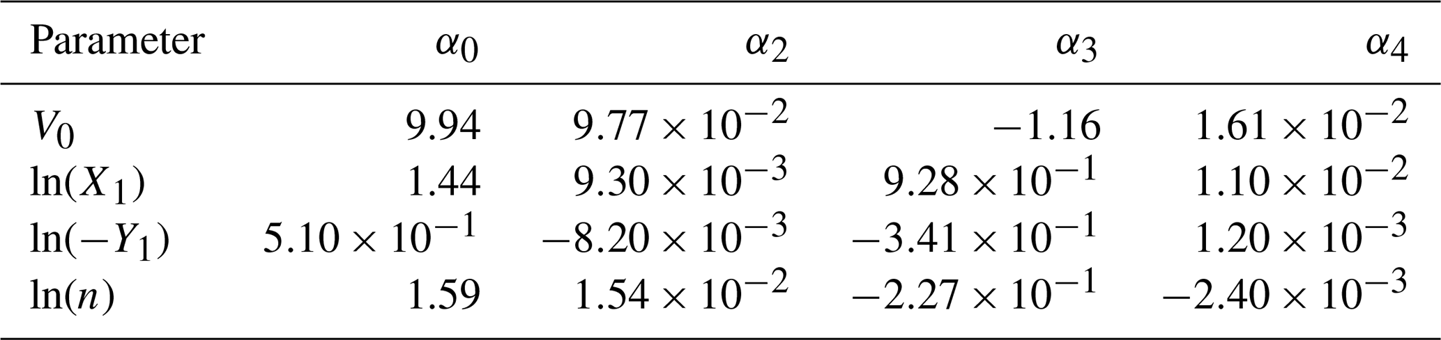
Table 1 presents the coefficients of the multi-linear regression obtained by Vinour et al. (2026).

Table 1 Results of the least-squares regression of the Loridan et al. (2015) model parameters, as given by Vinour et al. (2026).

The model of Loridan et al. (2015) provides the axisymmetric wind component of TCs. However, the actual wind field over open-ocean conditions is generally asymmetric, mainly due to the TC translation. An asymmetric component is therefore considered and described in the following.

2.1.2 Asymmetric wind model

The asymmetric wind field V_as is given by the formulation from Olfateh et al. (2017) with parameters also fitted on the SAR dataset by Vinour et al. (2026). The asymmetric wind V_as is given by

$$\begin{array}{}\text{(3)}& {\displaystyle }{\displaystyle }{V}_{\mathrm{as}}\left(r\right)=\mathit{ϵ}{V}_{\mathrm{m}}\sin (\mathit{\theta }+\mathrm{\Phi }){\left[\mathrm{e}{\left({\displaystyle \frac{R_a}{r}}\right)}^D{\mathrm{e}}^{-{\left(\frac{R_a}{r}\right)}^D}\right]}^{\mathrm{1}/\mathrm{2}},\end{array}$$

where θ is the azimuth in the TC reference frame centred on the TC direction of propagation. R_a is the distance to the maximum wind speed, D is the sharpness of the wind field, ϵ is the asymmetry parameter, and Φ is the azimuthal location of the maximum wind speed in the TC reference frame. The parameters are fitted on the same SAR dataset using a multi-linear regression of the parameters R_m, V_m, and C (translation speed) (Vinour et al., 2026).

The adjustable parameters p are expressed as

$$\begin{array}{}\text{(4)}& {\displaystyle }{\displaystyle }p={\mathit{\alpha }}_{\mathrm{0}}+{\mathit{\alpha }}_{\mathrm{1}}{V}_{\mathrm{m}}+{\mathit{\alpha }}_{\mathrm{2}}\ln \left(R_{\mathrm{m}}\right)+{\mathit{\alpha }}_{\mathrm{3}}C.\end{array}$$

The coefficients are gathered in Table 2.

Table 2 Results of the least-square regression of the Olfateh et al. (2017) model parameters, as given by Vinour et al. (2026).

Following Vinour et al. (2026), the azimuthal location of the maximum wind Φ is defined by a parameterised sectionally continuous linear profile depending on the normalised distance from the TC centre, $r/R_{\mathrm{m}}$:

$$\begin{array}{}\text{(5)}& {\displaystyle }{\displaystyle }\mathrm{\Phi }\left(r\right)=\left\{\begin{array}{ll}min\left(\mathrm{156.1}-\mathrm{185.6}\frac{r}{R_m},\mathrm{0}\right)& \text{; }r/R_{\mathrm{m}}<r_c\\ -\mathrm{54.1}-\mathrm{3.5}\frac{r}{R_m}& \text{; }r/R_{\mathrm{m}}\ge r_c\end{array}\right.,\end{array}$$

with r_c=1.154.

The asymmetric wind is added to the axisymmetric wind given by Eq. (1) to obtain the total surface wind.

The surface model is initialised using the maximum wind speed V_m, which is defined with different averaging periods depending on the meteorological agency. In the present study, V_m provided by the US agency is taken into account, which is a 1 min average wind speed (Knapp et al., 2010). However, the measurements considered in this paper are based on 10 min averaging. A conversion factor of 0.93 is thus applied to V_m to obtain consistent 10 min average wind speeds (Harper et al., 2010; Reul et al., 2017; Meissner et al., 2017).

2.1.3 Vertical extrapolation of surface wind to hub height

The above-described parametric model provides the surface wind field at 10 m above the sea level. However, for OWT design, wind speed at hub height (e.g. between 100 and 200 m, depending on the OWT power) is required. To do so, the surface wind is extrapolated using a logarithmic law assuming a neutral atmosphere:

$$\begin{array}{}\text{(6)}& {\displaystyle }{\displaystyle }U\left(z\right)={\displaystyle \frac{u^{*}}{\mathit{\kappa }}}\ln \left({\displaystyle \frac{z}{z_{\mathrm{0}}}}\right),\end{array}$$

with u^* the friction velocity, κ the von Kármán constant (=0.4), and z₀ the roughness length. The friction velocity is related to the surface shear through the drag coefficient C_d:

$$\begin{array}{}\text{(7)}& {\displaystyle }{\displaystyle }\mathit{\tau }=\mathit{\rho }{u}^{{*}^{\mathrm{2}}}=\mathit{\rho }{C}_{\mathrm{d}}{U}_{\mathrm{10}}^{\mathrm{2}},\end{array}$$

with ρ the air density and U₁₀ the mean wind speed at 10 $\mathrm{m}\mathrm{a}.\mathrm{s}.\mathrm{l}.$

The drag coefficient obtained from the WASP parameterisation (Bouin et al., 2024) is used in the present study. It provides a mean value among experimental data in TC conditions. Figure 1 displays its variation with the surface wind U₁₀ as well as the formulation used in the SWAN model (Zijlema and van der Westhuysen, 2005) employed in Larsén and Ott (2022) and the formulation recommended by DNV (2025). For comparison, the COARE 3.0 parameterisation of Fairall et al. (2003) based on the Charnock parameter is also displayed.

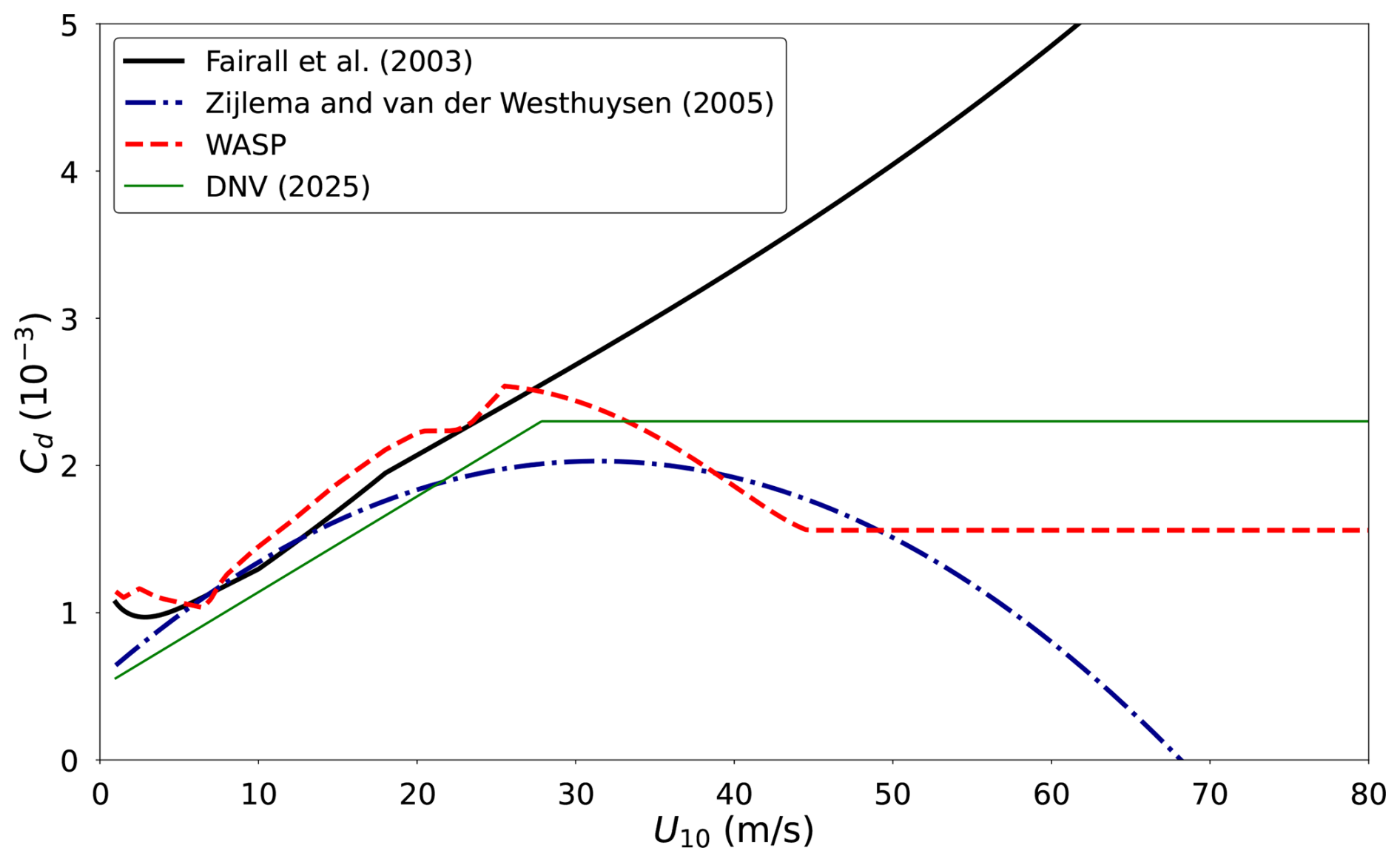
Figure 1 Drag coefficient as a function of surface wind speed U₁₀ for various parameterisations.

In Sect. 5, the accuracy of the logarithmic profile using the WASP drag coefficient is assessed with vertical wind profile measurements. The present model, hereafter referred to as OROWSHI model, is compared with the gradient wind formulation used in the Monte Carlo approach of Ishihara and Yamaguchi (2015).

2.2 Ishihara and Yamaguchi (2015) wind model (I&Y15)

For comparison, the wind model described in Ishihara and Yamaguchi (2015) (referred to in IEC, 2019) is implemented. The model relies on the gradient wind formula from Meng et al. (1995), which assumes that the pressure gradient force, given by Schloemer (1954)'s formulation, is balanced by the centrifugal and Coriolis forces. The gradient wind is then extrapolated to the altitude of interest using a power law (Meng et al., 1997). Ishihara and Yamaguchi (2015) considered a shear exponent of 0.1 for offshore applications. The shear exponent depends on the roughness length through an empirical formula in Ishihara and Yamaguchi (2015). For wind over terrain, the Global Land Cover dataset from Copernicus (Buchhorn et al., 2020) gives a 100 m resolution discrete classification of the type of soil. Each class is assigned a roughness length. The roughness length over sea is set to $\mathrm{1.6}\times {\mathrm{10}}^{-\mathrm{4}}$ m to match a shear exponent of 0.1 using the empirical formulation from Ishihara and Yamaguchi (2015). The averaging time of the wind speed from this parametric model applied to the best-track dataset is assumed to be a 3 h average (Yasui et al., 2002). In the present study, time series and surface wind fields at specific time steps are compared. For time series, the 3 h wind speed can be converted to 10 min average following the method described in Yasui et al. (2002), which is based on random realisations of a normal distribution. However, this method can not be applied to assess a wind field at a given instant. Therefore, for consistency in the averaging period for surface wind field comparisons and to obtain a consistent order of magnitude, the maximum 10 min wind speed is derived from the 3 h wind field by using the time conversion model described in Yamaguchi et al. (2012). The maximum M minute average wind speed $U_M^{\text{max}}$ to 10 min average $U_{\mathrm{10}\min }^{\text{max}}$ is computed from

$$\begin{array}{}\text{(8)}& {\displaystyle }{\displaystyle \frac{U_M^{\text{max}}}{U_{\mathrm{10}\min }^{\text{max}}}}=\mathrm{1}-\mathrm{0.0810}{\left({\displaystyle \frac{M-\mathrm{10}}{\mathrm{60}}}\right)}^{\mathrm{0.5457}},\end{array}$$

with M the number of minutes.

2.3 Local orographic effects

The surface and gradient wind models were derived assuming open-ocean conditions. However, upstream orography may disturb the wind flow in coastal regions. A standard practice for accounting for these effects is to compute a speed-up ratio that corrects the wind from the parametric model (Ishihara et al., 2005; Ishihara and Yamaguchi, 2015). The speed-up ratio is defined as the ratio between the wind computed over the actual orography and the wind speed over a flat surface of uniform roughness. The MASCOT software (Ishihara and Hibi, 2002) is used to derive the variation in the speed-up ratio with wind direction.

In Ishihara and Yamaguchi (2015), the wind direction is given by an empirical formulation, while the surface wind model of Vinour et al. (2026) provides no information on the actual wind direction. The wind direction is thus defined as the tangential direction corrected by an inflow angle. The inflow angle corresponds to the difference between the tangential direction relative to the TC centre and the actual surface wind direction. In this study, the inflow angle is fixed to −22.5° (Powell et al., 2009; Zhang and Uhlhorn, 2012; Tamizi et al., 2020) in the OROWSHI model for the application of the speed-up ratio.

To assess the limitations of the parametric models in coastal regions, their results are compared with those obtained from a mesoscale model and a reanalysis, which incorporate detailed physics, in particular, the effects of terrain and surface obstacles.

2.4 Mesoscale wind model and global reanalysis

For comparison with the parametric models, a mesoscale model and a global reanalysis dataset accounting for more physics are presented. Below is a brief description of the available data.

2.4.1 Wind fields from the Hurricane Weather Research and Forecasting Model – HWRF

The Hurricane Weather Research and Forecasting (HWRF) model from NOAA (National Oceanic and Atmospheric Administration) is a mesoscale ocean-coupled numerical weather prediction model designed specifically for tropical cyclone forecasting (Biswas, 2018). The data used in this study were provided by NOAA and consist of wind fields at a resolution of 0.015° (0.02° for events before 2018). HWRF is initialised either through data assimilation or using a bogus vortex approach. The model solves the non-hydrostatic Reynolds-averaged Navier–Stokes equations over time using the WRF model (Skamarock et al., 2019), producing forecasts at 3 or 6 h intervals. To minimise forecast errors and model drift from observations, only the first forecast outputs at 3 and 6 h lead times are used in this study. Vertical profiles are provided at isobaric levels, with the first level corresponding to surface winds (10 m above mean sea level). The second level is derived using the hypsometric equation:

$$\begin{array}{}\text{(9)}& {\displaystyle }{\displaystyle }{z}_{\mathrm{2}}=(\ln P_{\mathrm{1}}-\ln P_{\mathrm{2}})\left({\displaystyle \frac{R}{g}}T\right),\end{array}$$

with P₁=1000 hPa (first level), P₂=975 hPa (second level), R is the specific gas constant, g is the acceleration of gravity, and T is the air temperature (K).

In this study, HWRF wind fields are treated as 10 min average winds. Although the model output does not explicitly specify the temporal averaging period which depends on the model configuration and grid resolution, winds from mesoscale numerical weather prediction models, such as HWRF, correspond to time-averaged values rather than instantaneous gusts due to numerical filtering and space averaging (Harper et al., 2010). This assumption is supported by the model's use of parameterised subgrid turbulence and boundary-layer schemes, which inherently smooth high-frequency variability. Therefore, for consistency with the averaging time of the observations used in this study, HWRF winds are assumed to represent 10 min average values.

2.4.2 Wind fields from the European Centre for Medium-Range Weather Forecasts reanalysis version 5 – ERA5

The European Centre for Medium-Range Weather Forecasts reanalysis version 5 (ERA5) (Hersbach et al., 2023) uses data assimilation of observations and weather models to provide hourly estimates of atmospheric parameters on a horizontal grid of resolution 0.25° back to 1940. Wind speeds at 10 and 100 m are extracted during the cyclonic events. The ERA5 hourly wind estimates are converted to 10 min average wind using the with M=60.

2.4.3 Vertical extrapolation

Since both HWRF and ERA5 databases provide wind estimates at limited vertical levels, wind speeds must be extrapolated to the height of interest to ensure consistency with the measurements. In this study, the wind speed is assessed at a representative hub height of an offshore wind turbine, from ≈100 to 200 m depending on the data available. A power law is used to extrapolate the wind speed at the altitude of interest using the first two levels provided in HWRF and ERA5:

$$\begin{array}{}\text{(10)}& {\displaystyle }{\displaystyle }U\left(z\right)=U_{\mathrm{10}}{\left({\displaystyle \frac{z}{\mathrm{10}}}\right)}^{\mathit{\alpha }},\end{array}$$

with α the shear exponent, computed from the wind speeds at the two available altitudes:

$$\begin{array}{}\text{(11)}& {\displaystyle }{\displaystyle }\mathit{\alpha }={\displaystyle \frac{\ln U\left(z_{\mathrm{2}}\right)-\ln \left(U_{\mathrm{10}}\right)}{\ln z_{\mathrm{2}}-\ln \mathrm{10}}}.\end{array}$$

U(z₂) is the wind speed at the second altitude, z₂, corresponding to 100 m for ERA5 and ≈220 m for HWRF (T≈300 K for all time steps of the cases presented in the following).

3 IBTrACS data processing

To produce wind time series, best-track data are used as input to the parametric models presented in Sect. 2. In most studies, parametric models directly take into account the raw values provided by best-track datasets. However, some TC characteristics and parameters correspond to local values (e.g. derived from spatially distributed observations such as airborne radiometer, SAR images, or scatterometers) and are not consistent with the azimuthally averaged quantities (one-dimensional) required by the models. The processing of these parameters is therefore described in this section.

The IBTrACS dataset provides TC locations and characteristic parameters at a 3 h time step. First, the locations of the TC are interpolated at 10 min intervals using quadratic splines. The translation direction is derived from the interpolated locations. The TC characteristic parameters from the US agency are linearly interpolated along the tracks.

3.1 Maximum wind speed

The maximum wind speed from IBTrACS is local (two-dimensional) while the axisymmetric wind profile from Loridan et al. (2015) requires an azimuthally averaged V_m. In this study, the correction proposed by Vinour et al. (2026) is implemented to obtain an azimuthally averaged maximum wind, consistent with the parametric model. The relationship follows:

$$\begin{array}{}\text{(12)}& {\displaystyle }{\displaystyle }{V}_{\mathrm{m}}=\mathrm{0.8066}{V}_{\mathrm{IBTrACS}}+\mathrm{2.985},\end{array}$$

with V_IBTRrACS corresponding to the parameter USA_WIND in the best-track dataset.

3.2 Radius of maximum wind

An important parameter in the description of TCs is the radius of maximum wind R_m, which represents the distance from the TC centre to the location of the strongest winds. It is therefore a key parameter for accurately estimating wind speeds, especially when the TC is close to the site of interest. In most studies, R_m is used as provided in the best-track data. However, it is derived from the local (two-dimensional) maximum wind rather than azimuthally averaged quantities, which may introduce significant uncertainty in its use within parametric models.

Chavas and Knaff (2022) highlighted that R_m is difficult to measure and is badly resolved in models and reanalyses. Here, R_m is estimated from V_m, ϕ, and R₃₄ following the methodology of Chavas and Knaff (2022). The angular momentum is given by

$$\begin{array}{}\text{(13)}& {\displaystyle }{\displaystyle }{M}_a=rV+{\displaystyle \frac{\mathrm{1}}{\mathrm{2}}}f{r}^{\mathrm{2}},\end{array}$$

with r the radius, V the tangential wind speed, and f the Coriolis parameter.

Knowing the ratio $M_a(r=R_{\max })/M_a(r=R_{\mathrm{34}})$, R_m can be computed as follows:

$$\begin{array}{}\text{(14)}& {\displaystyle }{\displaystyle }{R}_{\mathrm{m}}={\displaystyle \frac{V_{\mathrm{m}}}{f}}\left(\sqrt{\mathrm{1}+{\displaystyle \frac{\mathrm{2}f{M}_a(r=R_{\max })}{V_{\mathrm{m}}^{\mathrm{2}}}}}-\mathrm{1}\right).\end{array}$$

Avenas et al. (2023) computed the ratio $M_a(r=R_{\max })/M_a(r=R_{\mathrm{34}})$ from an SAR–radiometer collocation dataset and derived the following parameterisation, adopted here:

$$\begin{array}{ll}{\displaystyle }& {\displaystyle }{M}_a(r=R_{\max })/M_a(r=R_{\mathrm{34}})=\mathrm{0.531}\\ {\displaystyle }& {\displaystyle }\times \exp [-\mathrm{0.00214}(V_{\mathrm{m}}-\mathrm{17.5})\\ \text{(15)}& {\displaystyle }& {\displaystyle }-\mathrm{0.00314}(V_{\mathrm{m}}-\mathrm{17.5})\left({\displaystyle \frac{\mathrm{1}}{\mathrm{2}}}f{R}_{\mathrm{34}}\right)].\end{array}$$

In the IBTrACS dataset, R₃₄ is available for the TC four quadrants. The mean value of R₃₄ is used to consistently obtain an axisymmetric R_m. The parameterisation (Eq. 15) was obtained with a 1 min azimuthally average wind speed. The intensity V_m from IBTrACS corrected by Eq. (12) is used to estimate R_m in Eqs. (14) and (15).

In Ishihara and Yamaguchi (2015), R_m is fitted from measured sea surface pressure, but no pressure measurements are available on the site of this study. Since the equation of Schloemer (1954) is an axisymmetric pressure model which requires an azimuthal average R_m, R_m obtained from the abovementioned methodology is used. Note that the current implementation differs from the original study from Ishihara and Yamaguchi (2015) as parameters from the Japan Meteorological Agency (JMA) were used, restricting the application to the Western Pacific basin. In particular, R_m is not provided by the JMA. In this study, the TC parameters from the US agency are used. Since they are provided for almost every TC, the current implementation is applicable anywhere.

3.3 Pressure

The I&Y15 model also requires the ambient pressure to apply the equation of Schloemer (1954), taken to 1013 hPa here (IEC, 2019). The USA_PRES parameter from the IBTrACS dataset gives the central pressure, which is used to quantify the central pressure depth.

4 Site description

The wind speeds obtained with the four models presented in Sect. 2 are compared at sites which were impacted by tropical cyclones along the US East Coast and in the Western Pacific. The site locations and the observed TCs are described in the following section.

4.1 Japan

A lidar located on Tairajima Island (33.70° N, 129.62° E) recorded winds from Typhoon Hinnamnor and Nanmadol (2022) on 20 vertical levels from 50 to 285 m. Only measurements at 95 and 205 m are considered for comparison with wind models. The locations of the TCs provided by IBTrACS are represented in Fig. 2. The wind intensity V_m from the US agency is presented for each location. The minimum distance from the TC centre to the site is 2.8 R_m and 1.0 R_m for Typhoon Hinnamnor and Nanmadol, respectively.

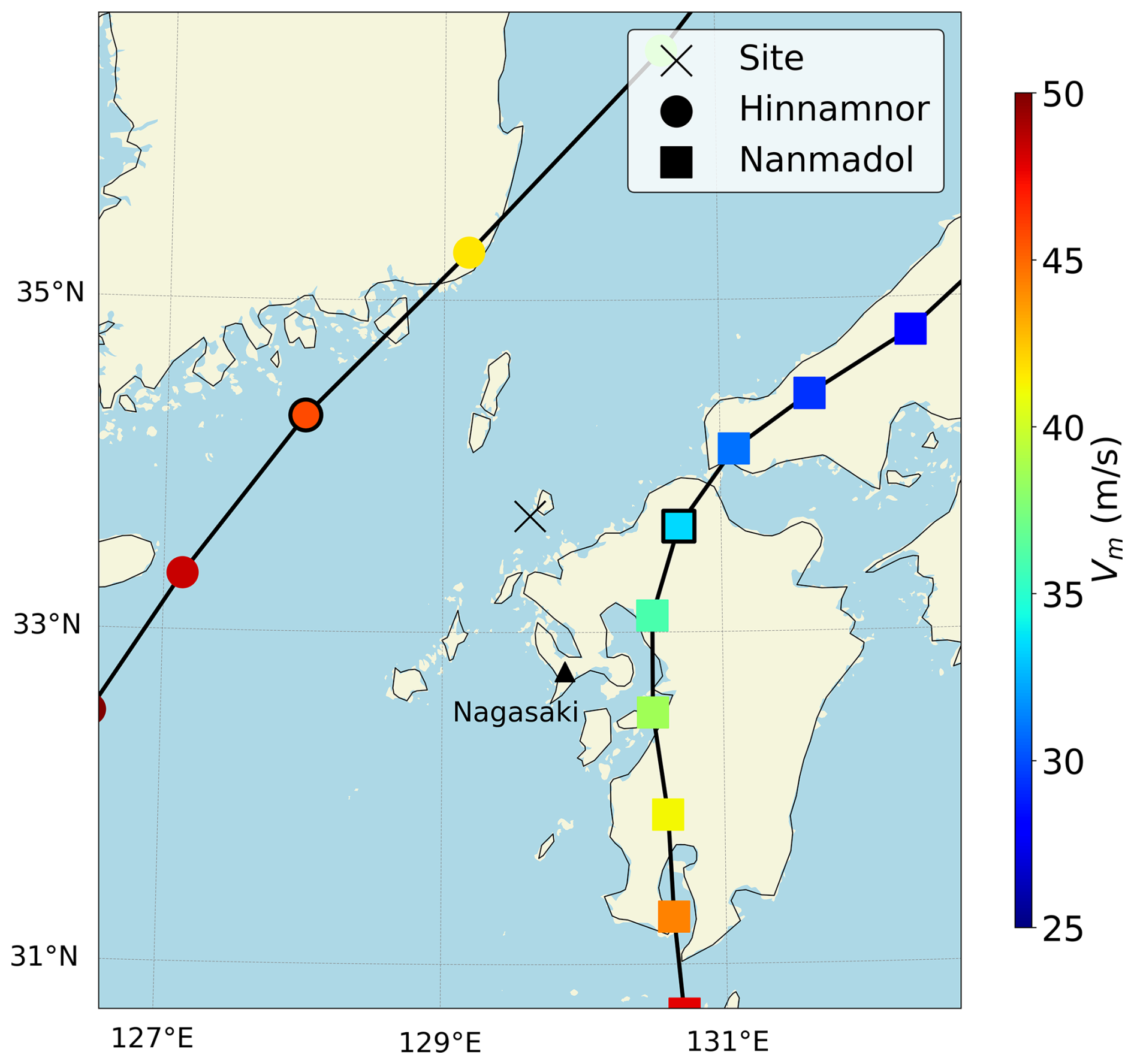
Figure 2 Measurement site (X) impacted by Typhoon Hinnamnor (•) and Nanmadol (▪) (both in 2022). The black outline on the marker highlights the location closest to the site.

The site is relatively close to Iki Island (≈5 km). Thus, local orographic effects may affect the wind. The variation in the speed-up ratio with wind direction (true north convention) is presented in Fig. 3. MASCOT software predicts a decrease in wind direction between 0–90°, due to Iki Island, while Kyushu Island affects the wind speed from 90 to 225°.

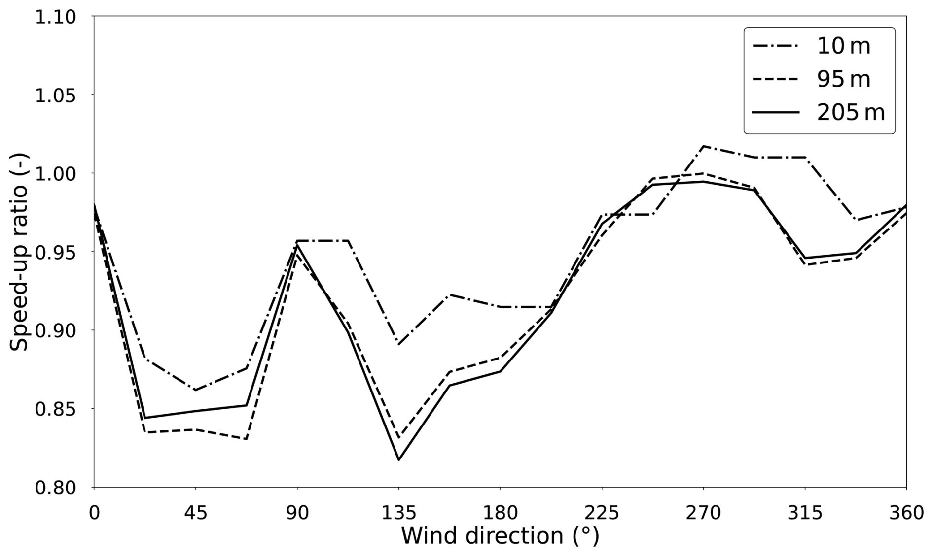
Figure 3 Variation in the speed-up ratio with wind direction at 10, 95, and 205 m above the mean sea level, computed using the MASCOT software.

4.2 New York Bight

A floating lidar located at 39.55° N, 73.43° W recorded the winds of Hurricane Isaias (2020). Figure 4 displays the TC track and wind intensity. The TC passed about 2.0 R_m from the site. During the event, two of the four quadrants of the TC are overland, with values of R₃₄ very low compared to those over sea. Since the present study aims at evaluating the performance of the parametric models over the sea, only the mean R₃₄ of the eastern quadrants is used for this case. The vertical discretisation of the measurements is 20 m from 18 to 198 m. The altitudes 98 and 198 m are used as reference for the comparison of the wind speed.

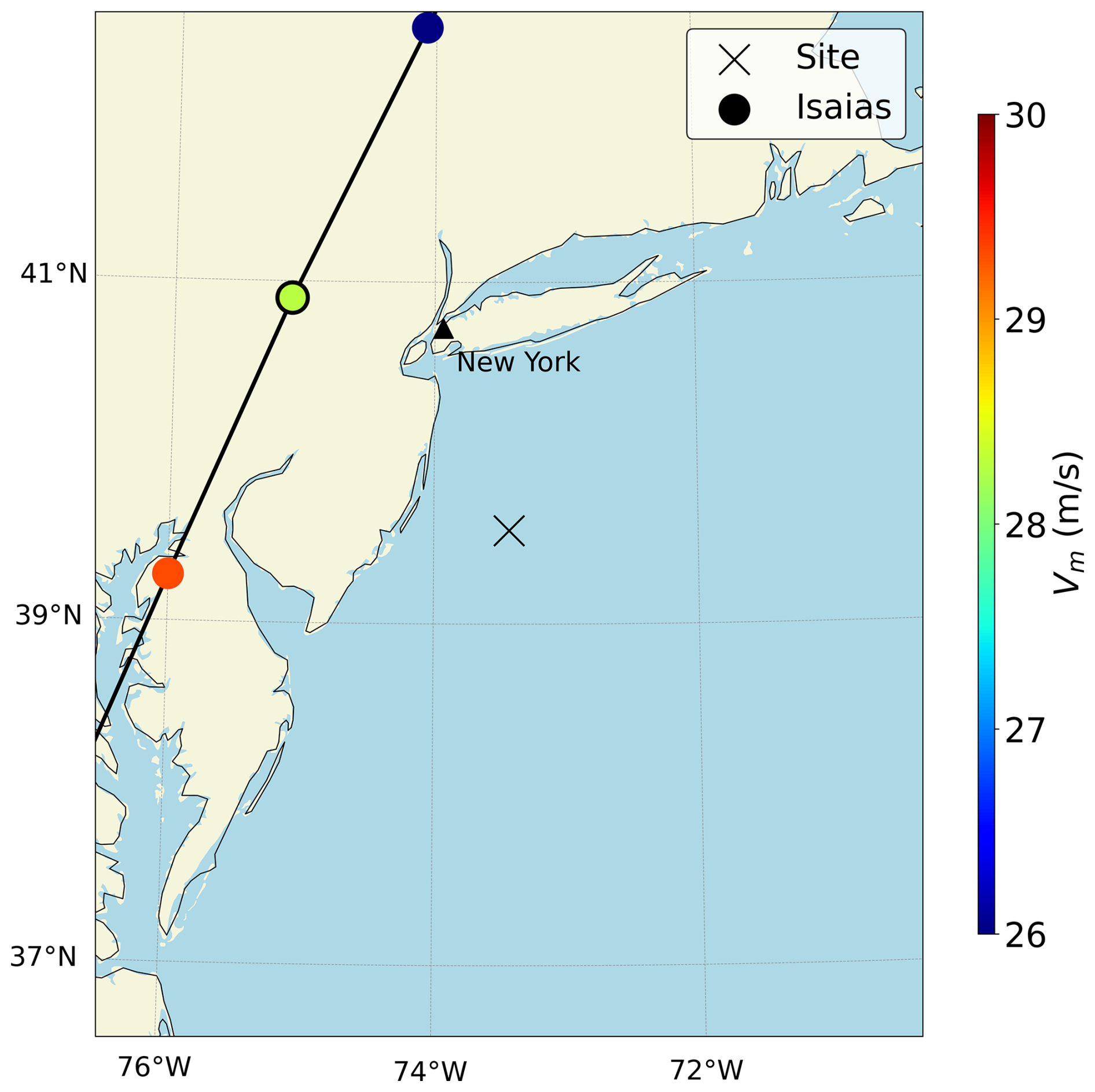
Figure 4 Measurement site (X) impacted by Hurricane Isaias (•) (2020).

The site is over 60 km from the coast. In this case, orographic effects are neglected.

4.3 Taiwan

Taiwan is hit by numerous typhoons every year. With mountains over 3 km high, this island is of particular interest for studying the interactions of tropical cyclones with mesoscale orography (e.g. Wu et al., 2015; Tang and Chan, 2016; Hsu et al., 2018; Müller et al., 2024a).

4.3.1 Site 1

The Formosa 1 is an offshore steel lattice meteorological mast installed on a fixed offshore structure at 24.71° N, 120.83° E. It is equipped with cup anemometers and wind vanes installed at 20 m intervals between 30 and 90 m above mean sea level. The tracks of TC Dujuan (2015) and Megi (2016) are presented in Fig. 5. The minimum distance of Dujuan from the site is 1.6 R_m and 1.0 R_m for Megi.

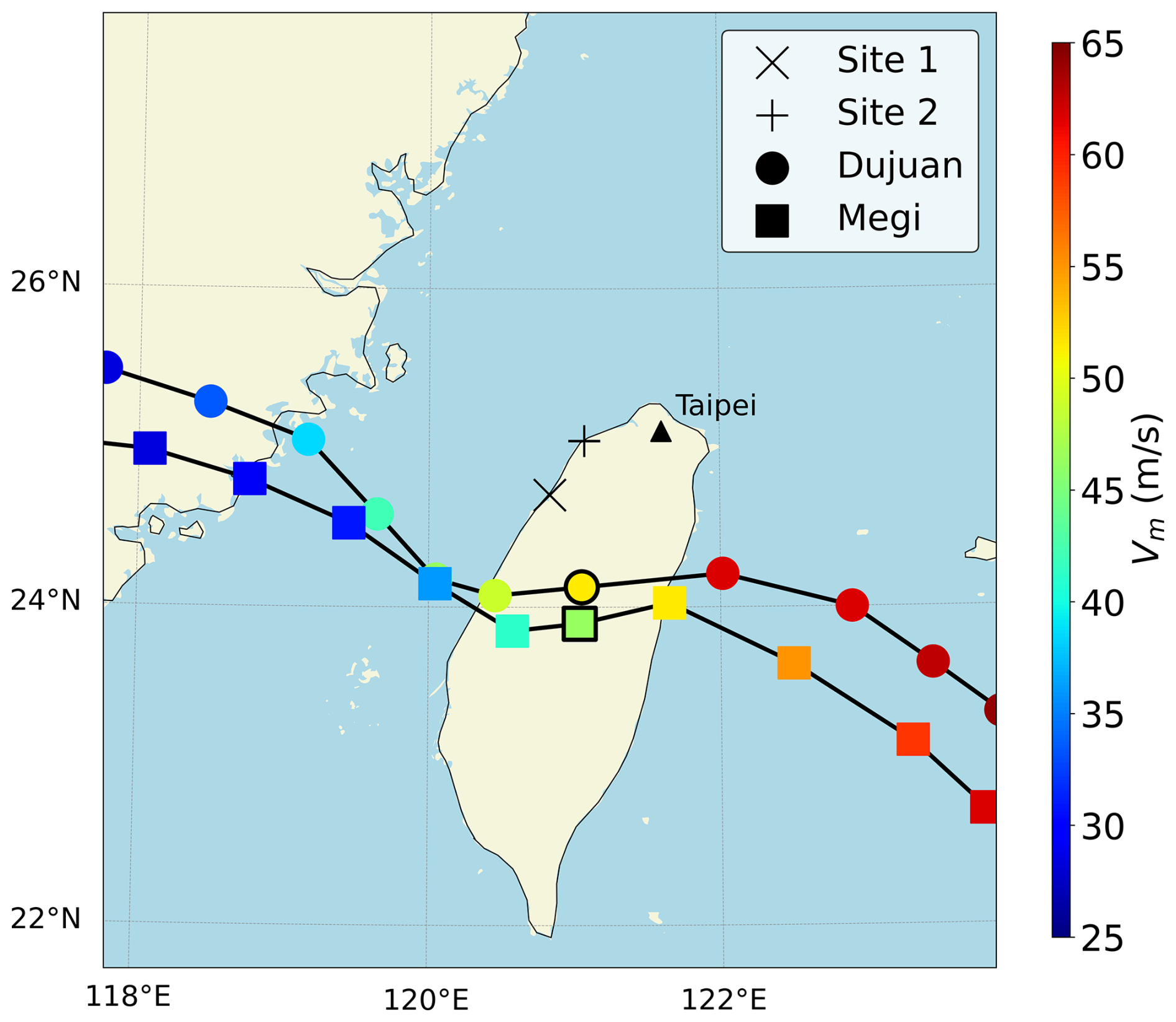
Figure 5 Measurement sites impacted by Typhoon Dujuan (sites: × and +, track: •) (2015) and Megi (site: +, track: ▪) (2016).

4.3.2 Site 2

The Guanyin meteorological mast is a steel lattice tower located along the shoreline at 25.04° N, 121.07° E. Five Thies First Class Advanced cup anemometers are installed between 50 m and 105 $\mathrm{m}\mathrm{a}.\mathrm{g}.\mathrm{l}.$ Winds from TC Megi (2016) were recorded.

Estimating a speed-up ratio to account for local orographic effects is challenging for such a large island as Taiwan. Indeed, the domain size is usually a few 10 km within MASCOT, which is enough when evaluating the flow over a relatively low orography, such as in the site studied in Ishihara and Yamaguchi (2015), characterised by rather close low-lying small-scale orographic obstacles. Wind flow over large mountain islands, such as Taiwan, is disturbed on a much larger scale, and the whole TC structure is affected. In such cases, steady-state CFD with idealised inflow is not appropriate, as they assume horizontally homogeneous and stationary upstream flow. There are alternatives to CFD for taking orographic effects into account, such as design codes, e.g. British Standards Institution (2005) used in Tan and Fang (2018), but Taiwan is also outside the scope of these methods. Consequently, orographic effects are not taken into account in these cases.

The five tropical cyclones analysed in this study cover a wide range of intensities, from Category 1 hurricane (Isaias) to Category 4-equivalent typhoon (Megi). Despite the limited number of TC studied, the range of intensities covered provides a relevant basis for evaluating the models under different wind intensities.

5 Application – vertical extrapolation

This section presents the assessment of the vertical wind distribution. First, the logarithmic law and the WASP drag coefficient are evaluated and compared to the measurements. Then, the shear exponent of the power law is derived using all available vertical levels. Only strong wind events (U₁₀>25 m s⁻¹) are analysed to not account for wave growth and keep only cyclonic events.

5.1 Assessment of the logarithmic law

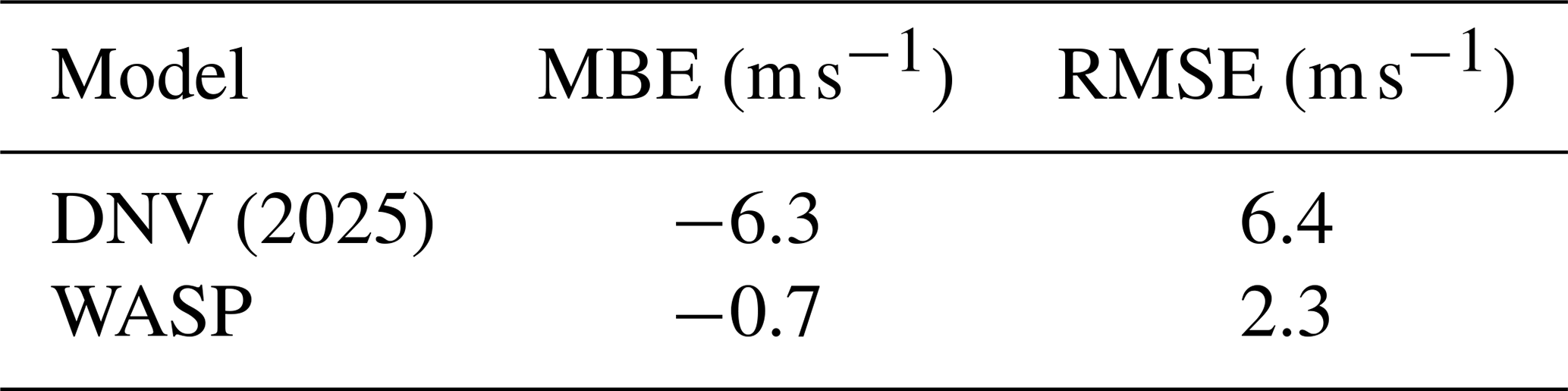
The surface wind speed and the drag coefficient are derived from a least-squares linear fitting as in Powell et al. (2003) for each sample. $u^{*}/\mathit{\kappa }$ is given by the slope and z₀ by the intercept on a log height scale. The surface wind U₁₀ is derived from Eq. (6) and the drag coefficient from Eq. (7). Figure 6 displays the drag coefficient computed for each sample from the 10 min mean wind speed. The observations are highly scattered and site-dependent. The dispersion of the results could in part be due to the difference in measurement heights across the various sites but also to upstream terrain affecting the vertical wind profiles. The drag coefficient derived from TC Megi (2016) is significantly different depending on the site, with a ratio of 2 between the two sites for U₁₀>30 m s⁻¹. This discrepancy may be attributed either to upstream topographic effects or to differences in wave conditions within the Taiwan Strait. The WASP and DNV (2025) formulations are presented for comparison. The two parameterisations are consistent with the mean value, which does not vary substantially for this wind speed range. Table 3 presents the mean bias error (MBE) and root mean square error (RMSE) of wind speed computed at 200 m (corresponding to hub height of 25 MW OWT Escalera et al., 2022) using WASP drag coefficient and DNV's recommendations. The reference value is computed from the fitted log law since level 200 m is not available in the data. The lowest errors are obtained with WASP for the analysed data. Extreme wind speeds at hub height are thus better estimated on average using the WASP drag coefficient than the DNV recommendation for this dataset.

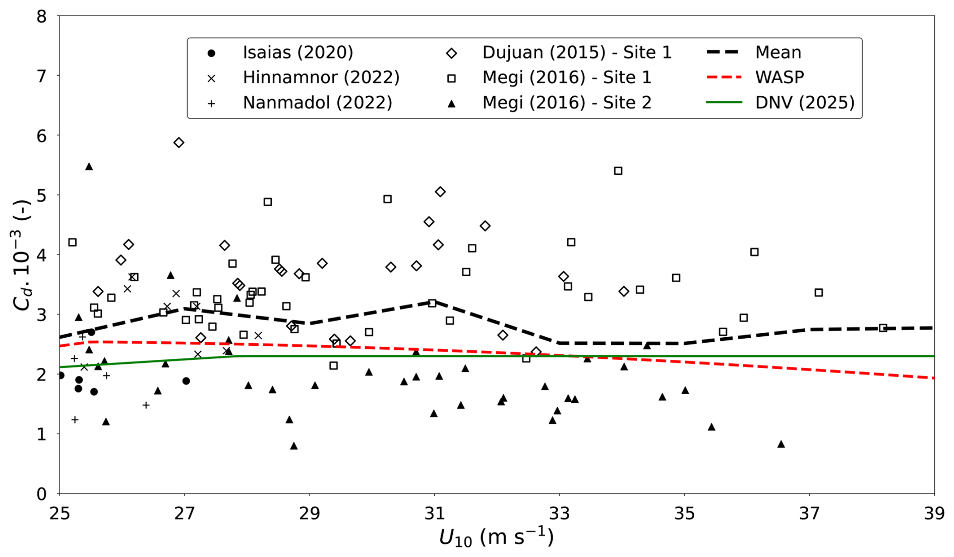
Figure 6 Drag coefficient as a function of surface wind U₁₀. Comparison between WASP, DNV (2025), and the measurements. The dashed black line corresponds to the mean measured value for bins of 2 m s⁻¹.

Table 3 Scores of wind speed at 200 m using log laws.

5.2 Assessment of the power law

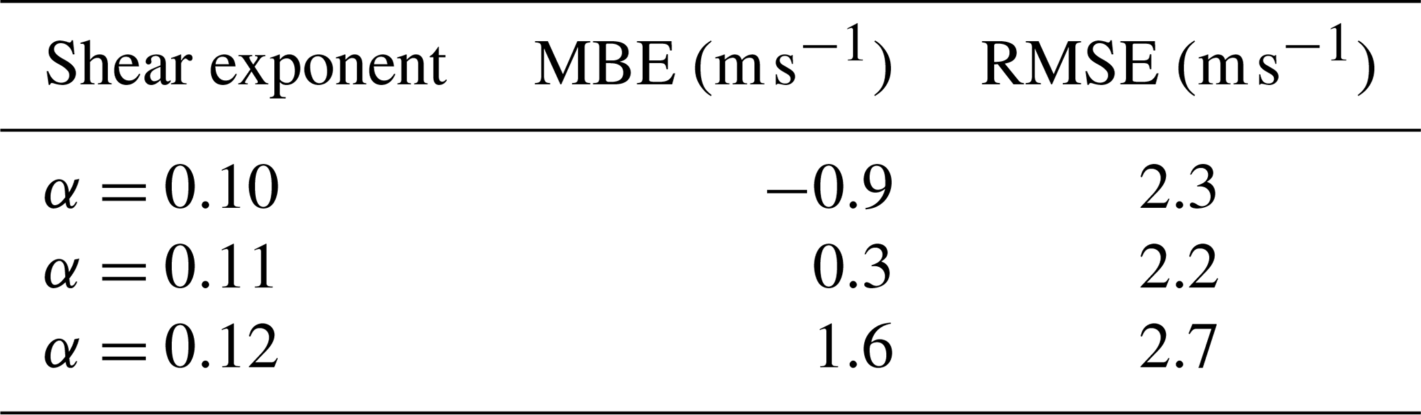
The power law (Eq. 10) is also widely used in the industry to extrapolate wind speed. DNV (2025) suggests using an exponent α=0.12 for open-ocean conditions with waves. In Ishihara and Yamaguchi (2015), α is set to 0.10. Recommendations from IEC (2019) suggest extrapolating the 50-year extreme wind speeds using α=0.11. The shear exponent is derived from the measurement using all available vertical levels to assess the reliability of the various proposed values.

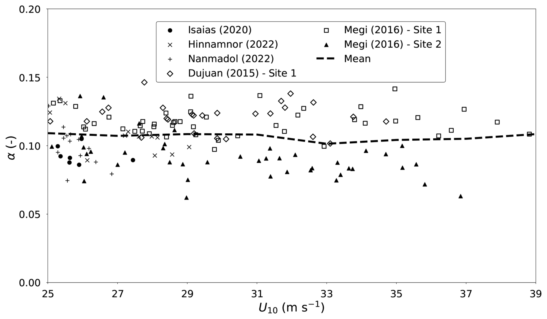
A power law is fitted to the vertical profiles with U₁₀ and shear exponent α as free parameters. Figure 7 presents the variation in the shear exponent with the surface wind. There is no significant variation in the mean value of α as a function of U₁₀, which is equal to 0.106. The median is 0.107, slightly higher than the value reported in Müller et al. (2024a). Table 4 presents the MBE and RMSE of wind speed computed at 200 m using shear exponents from 0.10 to 0.12. IEC's recommendations give the best results for this dataset. Although the power law with a shear exponent α=0.11 performs slightly better, the logarithmic law based on the WASP drag coefficient is retained for its stronger physical basis and interpretability.

Figure 7 Wind shear exponent α as a function of surface wind U₁₀.

Table 4 Scores of wind speed at 200 m using power laws.

6 Application – wind time series

This section compares the wind speeds predicted by the models with the measurements. The MBE and RMSE are computed for each event on the time series of the measured 10 min average wind speed. Moreover, the parametric models are to be used within the framework of a Monte Carlo approach. Generally, the location of the tropical cyclone centre is linearly extrapolated in time from the closest TC position from the site and using the direction of propagation (Vickery and Twisdale, 1995; Ishihara et al., 2005). In the end, only the maximum wind induced by each TC at the site is used to derive extreme wind statistics. It is therefore necessary to assess the ability of the models to capture the maximum wind at a given site. The percent deviation from the maximum measured wind (PD_max) is thus evaluated. In addition, surface wind fields centred on the best-track location are presented at relevant time steps, chosen to represent both peak wind conditions and configurations in which TCs are strongly affected by orography. Note that the HWRF wind field is a forecast. Thus, the TC centre may deviate from the location provided in IBTrACS.

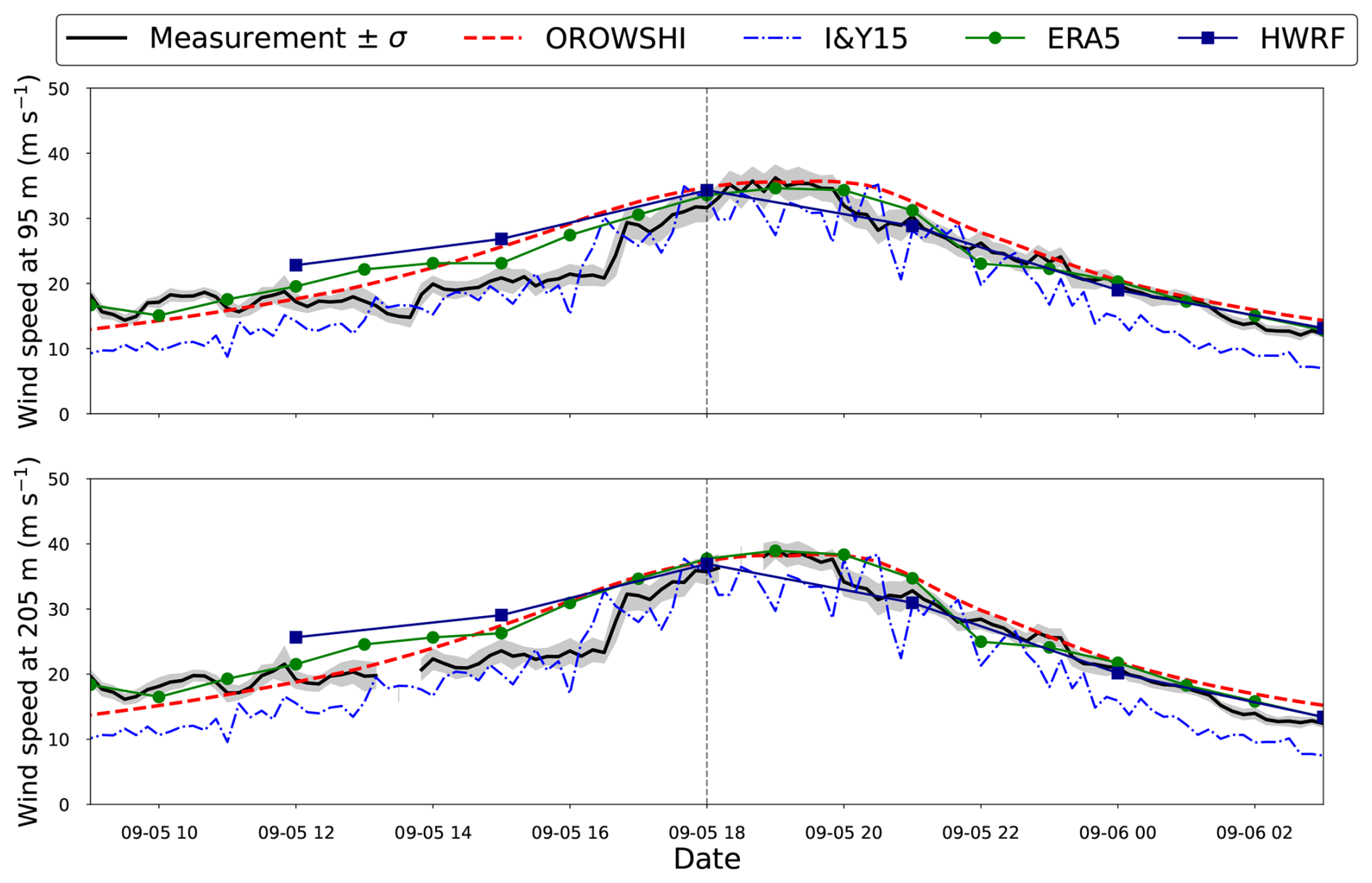
Figure 8 Time series of observed and predicted winds of TC Hinnamnor at 95 m (top panel) and 205 m (bottom panel). The vertical dashed line corresponds to the instant at which the surface wind field is assessed.

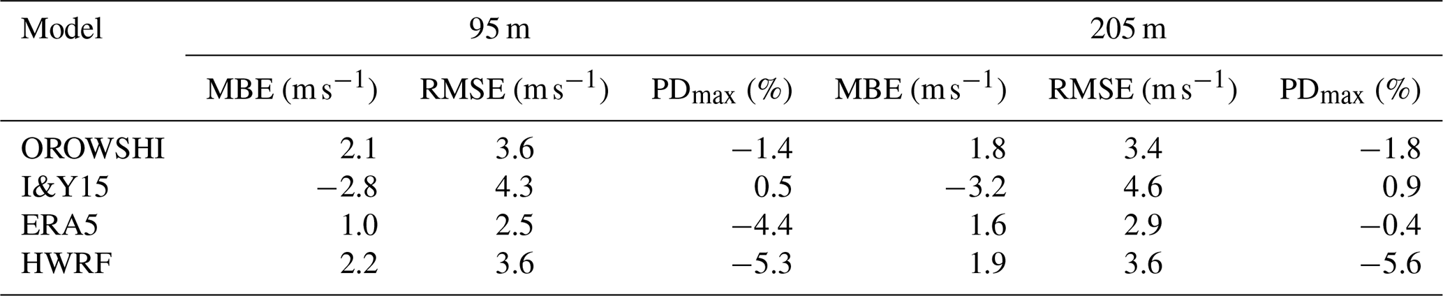
Table 5 Scores of the wind models for TC Hinnamnor at 95 and 205 m.

6.1 Typhoon Hinnamnor (2022)

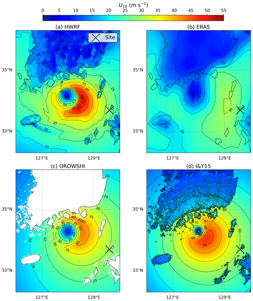
Wind time series from TC Hinnamnor are presented in Fig. 8. All the methods presented here align well with the observations. The scores of the wind speed predicted by the parametric models are similar to those obtained with ERA5 and HWRF and remain low (|MBE|<3 m s⁻¹ and RMSE<5 m s⁻¹; see Table 5). In this configuration, the parametric models are able to accurately capture the peak wind speed (|PD_max|<2 %), while HWRF slightly underestimates it due to its coarse temporal output sampling (${\text{PD}}_{\max }<-\mathrm{5}$ %). The surface wind field estimated by the four models on 5 September at 18:00 GMT is presented in Fig. 9. This time instant corresponds to the HWRF time step closest to the instant of the maximum wind speed measured at the site. Parametric models predict an eyewall spot similar to that of HWRF (Fig. 9a). ERA5 (Fig. 9b) shows lower wind speeds in the inner core compared to HWRF. This is due to its coarse horizontal resolution but also to inadequate physics parameterisations for cyclonic conditions (Xu et al., 2024). The apparent good agreement of the weak winds between ERA5 and HWRF in the outer area may be coincidental. HWRF is expected to perform better in representing the inner-core structure, but a comparison with measurements would be necessary to evaluate the accuracy of both models.

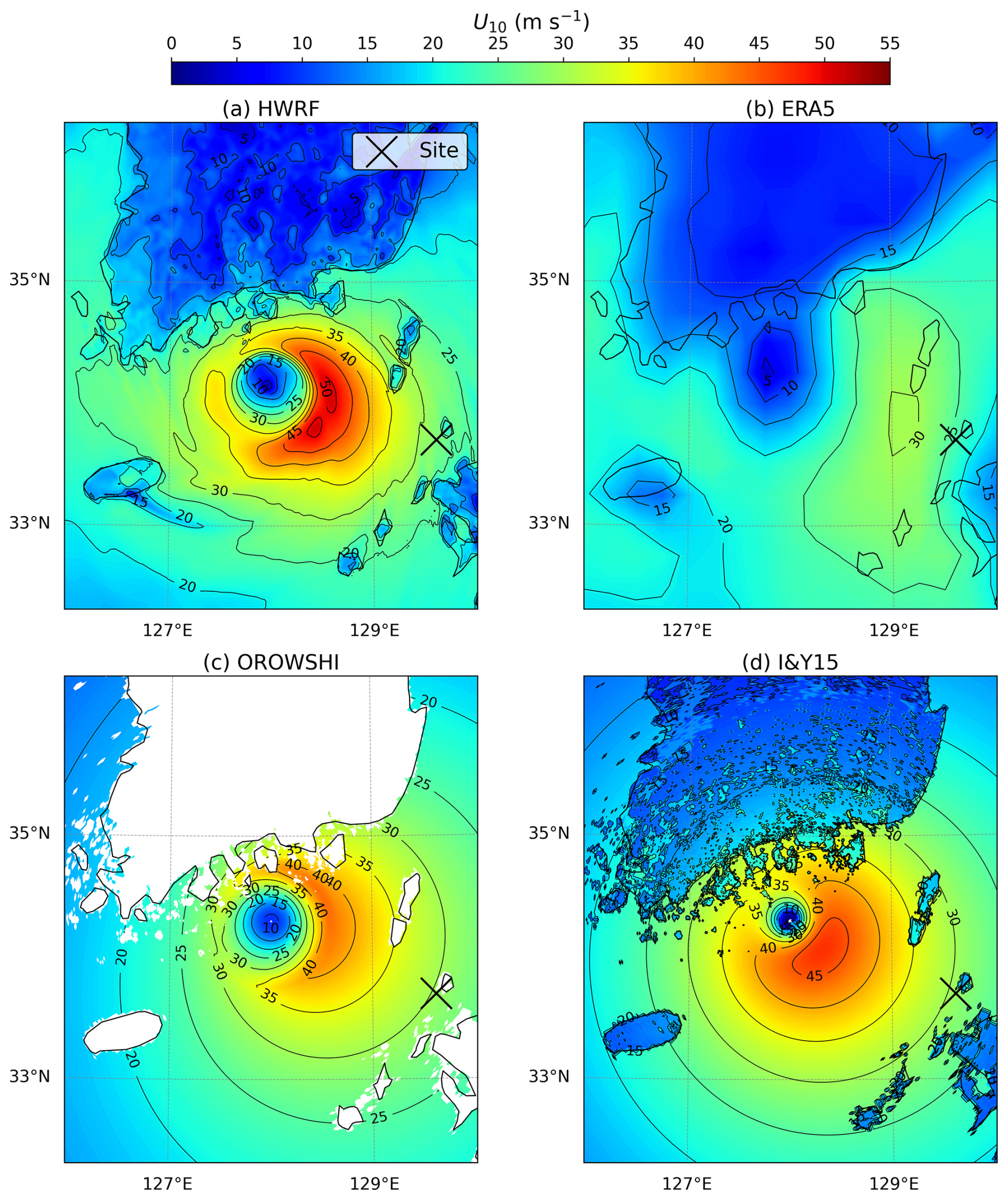
Figure 9 TC Hinnamnor surface wind field on 5 September at 18:00 GMT predicted by HWRF (a), ERA5 (b), OROWSHI wind model (c), and I&Y15 wind model (d).

The formulation used in Ishihara and Yamaguchi (2015) always predicts the location of the azimuth of maximum wind at 90° on the right-hand side of the direction of TC propagation (41° here) (Fig. 9d), which is reasonable at this specific instant. However, the area of high wind is larger than that predicted by HWRF and by the OROWSHI model, which could lead to different sea states in this area when the wind field forces a wave model.

The two parametric models satisfactorily predict the peak winds. Although both models are based on IBTrACS parameters, they differ in their primary inputs: the OROWSHI model is driven by V_m (Eq. 12), whereas I&Y15 depends on the central pressure depth. The maximum wind speeds predicted by the two models at a given instant are not necessarily the same.

6.2 Typhoon Nanmadol (2022)

Figure 10 presents the comparison of the wind speeds induced by TC Nanmadol. The parametric models underestimate the wind speed during the TC approaching phase by a factor of 2, which is a source of large errors in terms of RMSE (RMSE>5 m s⁻¹; see Table 6). Nevertheless, the peak wind speed and the wind during the leaving phase are quite well predicted, with a PD_max lower than 6 % from the measurements at the two altitudes. The surface wind fields on 18 September at 09:00 GMT are presented in Fig. 11. The TC begins to make landfall on Ky$\overline{\text{u}}$sh$\overline{\text{u}}$ Island at this instant. HWRF results (Fig. 11a) show that the high-wind spot is located opposite to the direction of TC direction (357° at this instant). The observed asymmetry is certainly due to the island perturbing the flow, which can not be represented by the OROWSHI model as it relies on SAR images over open-ocean conditions. Note that the radius of the eyewall predicted by the present implementation of the I&Y15 model is also much larger in this case, leading to a more extensive area of high wind speeds (>30 m s⁻¹) than those predicted by HWRF and the OROWSHI model.

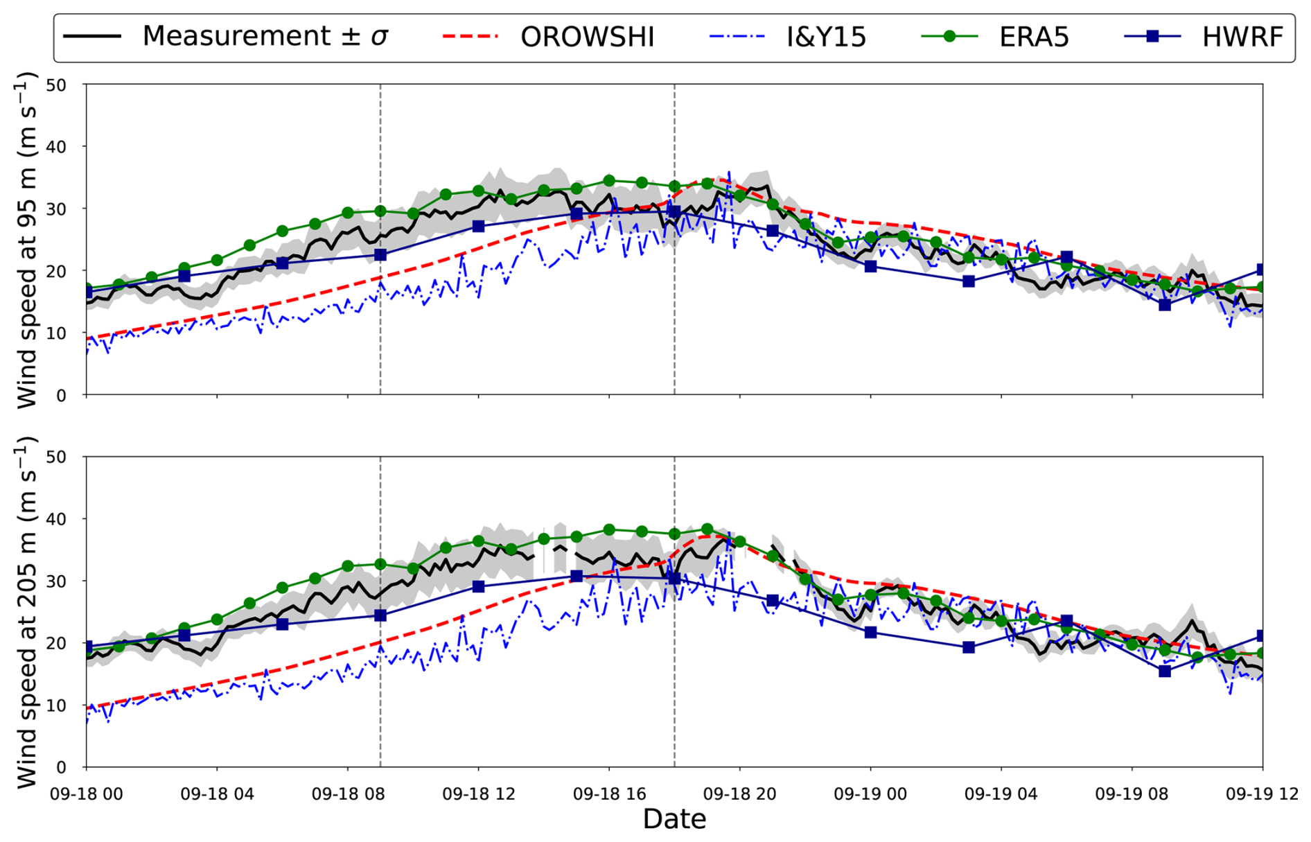
Figure 10 Time series of observed and predicted winds of TC Nanmadol at 95 m (top panel) and 205 m (bottom panel). The vertical dashed lines correspond to the instants at which the surface wind field is assessed.

Table 6 Scores of the wind models for TC Nanmadol at 95 and 205 m.

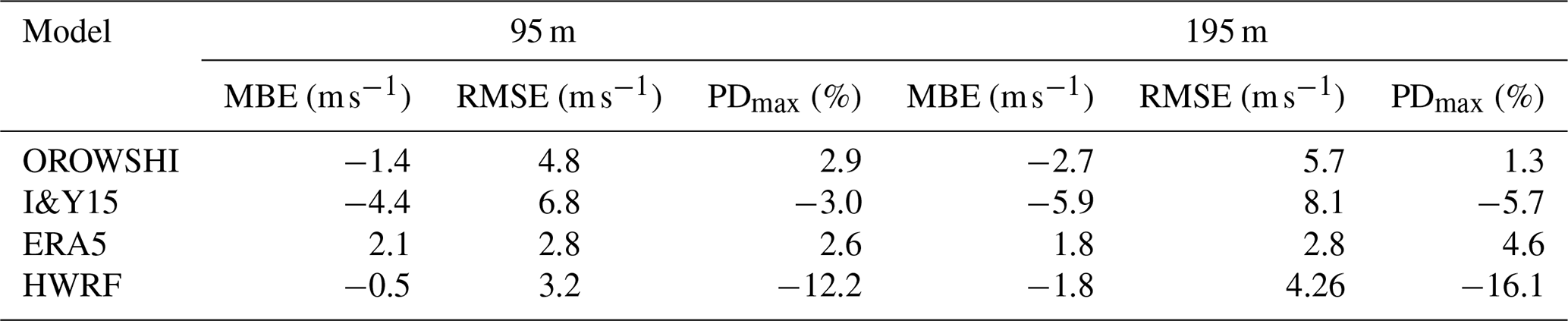
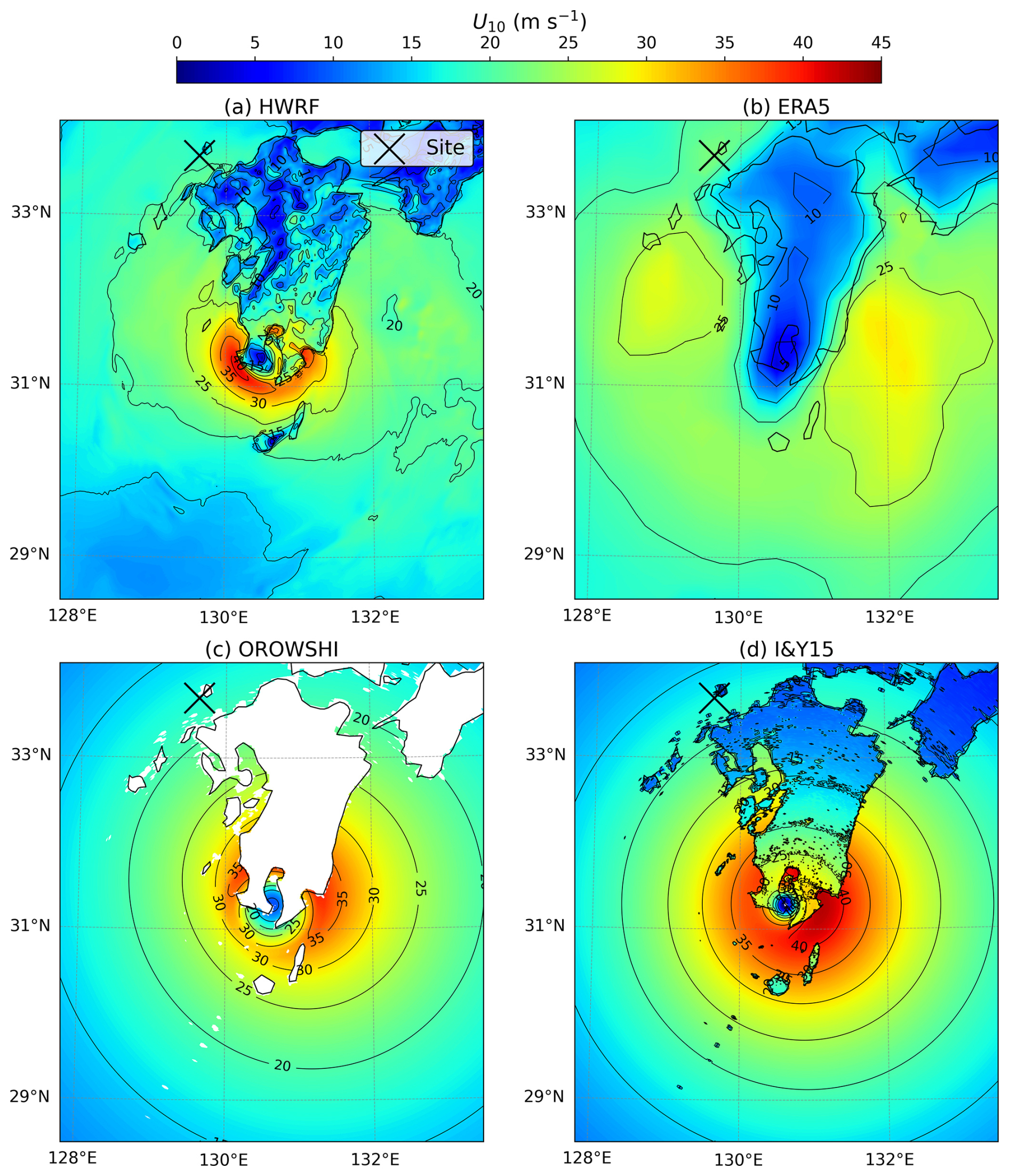
Figure 11 TC Nanmadol surface wind field on 18 September at 09:00 GMT predicted by HWRF (a), ERA5 (b), OROWSHI wind model (c), and I&Y15 wind model (d).

The surface wind fields during landfall on 18 September at 18:00 GMT are presented in Fig. 12. The OROWSHI model (Fig. 12c) is not designed to predict such a configuration when the TC is mainly over land. The area of high winds predicted by HWRF and by the OROWSHI model is located just around Kyushu Island's northern part, while the surface wind from the I&Y15 model is rather axisymmetric.

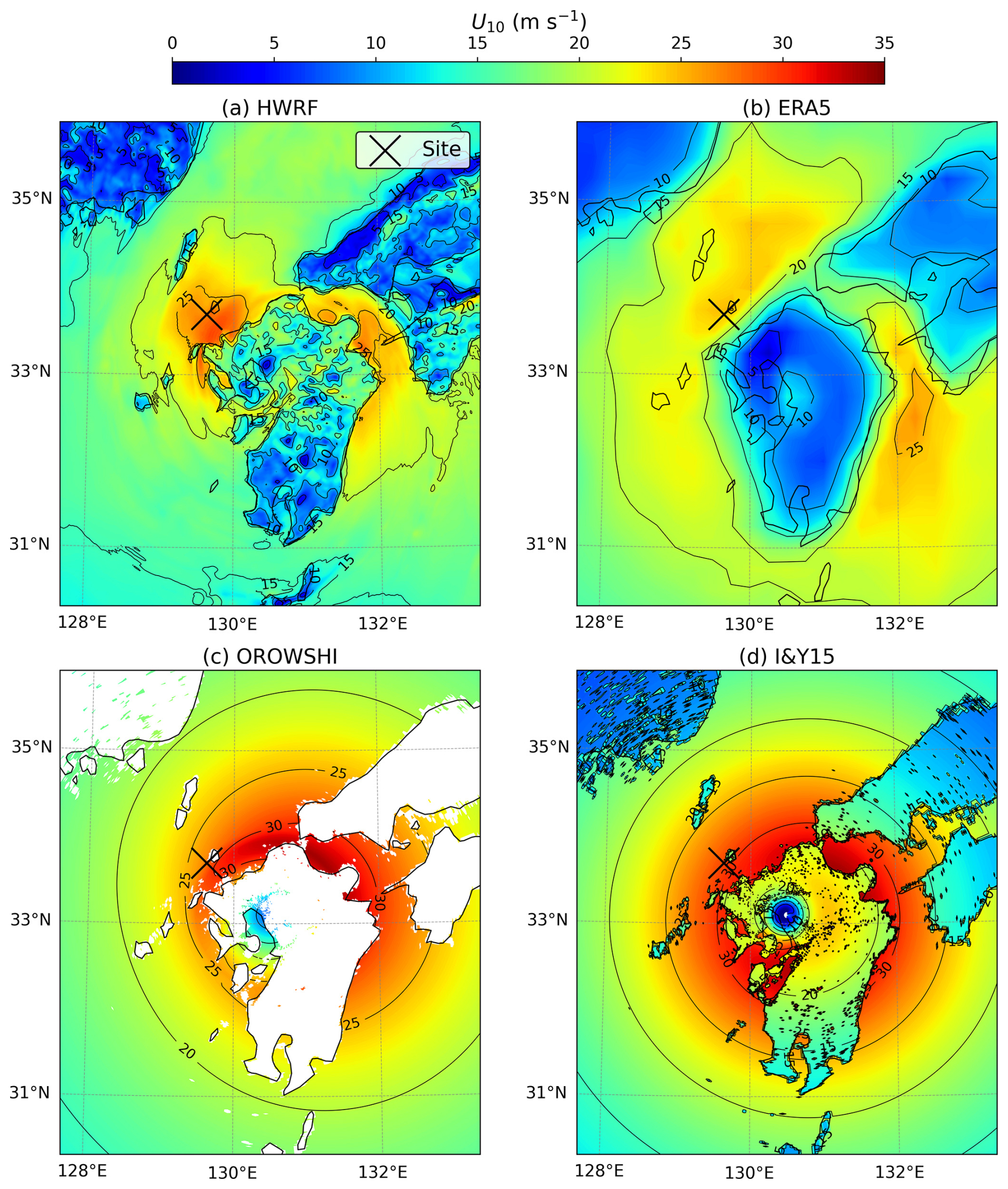
Figure 12 TC Nanmadol surface wind field on 18 September at 18:00 GMT predicted by HWRF (a), ERA5 (b), OROWSHI wind model (c), and I&Y15 wind model (d).

6.3 Hurricane Isaias (2020)

The wind time series of TC Isaias is displayed in Fig. 13. The OROWSHI model shows a reasonable agreement with the measurements with low MBE and RMSE (less than 5 m s⁻¹; see Table 7), but all models underestimate the main wind peak by at least 4 %. Note that HWRF accurately reproduces the measured wind speeds at the available output times. However, the 3 h output interval is too coarse to capture the maximum wind speed for this event. The winds from I&Y15 largely underestimate the measurements during the whole event with MBE and RMSE larger than 8 m s⁻¹.

Table 7 Scores of the wind models for TC Isaias at 98 and 198 m.

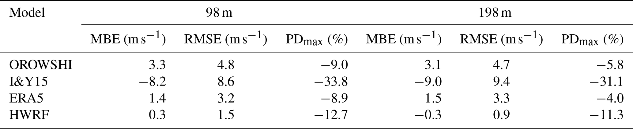
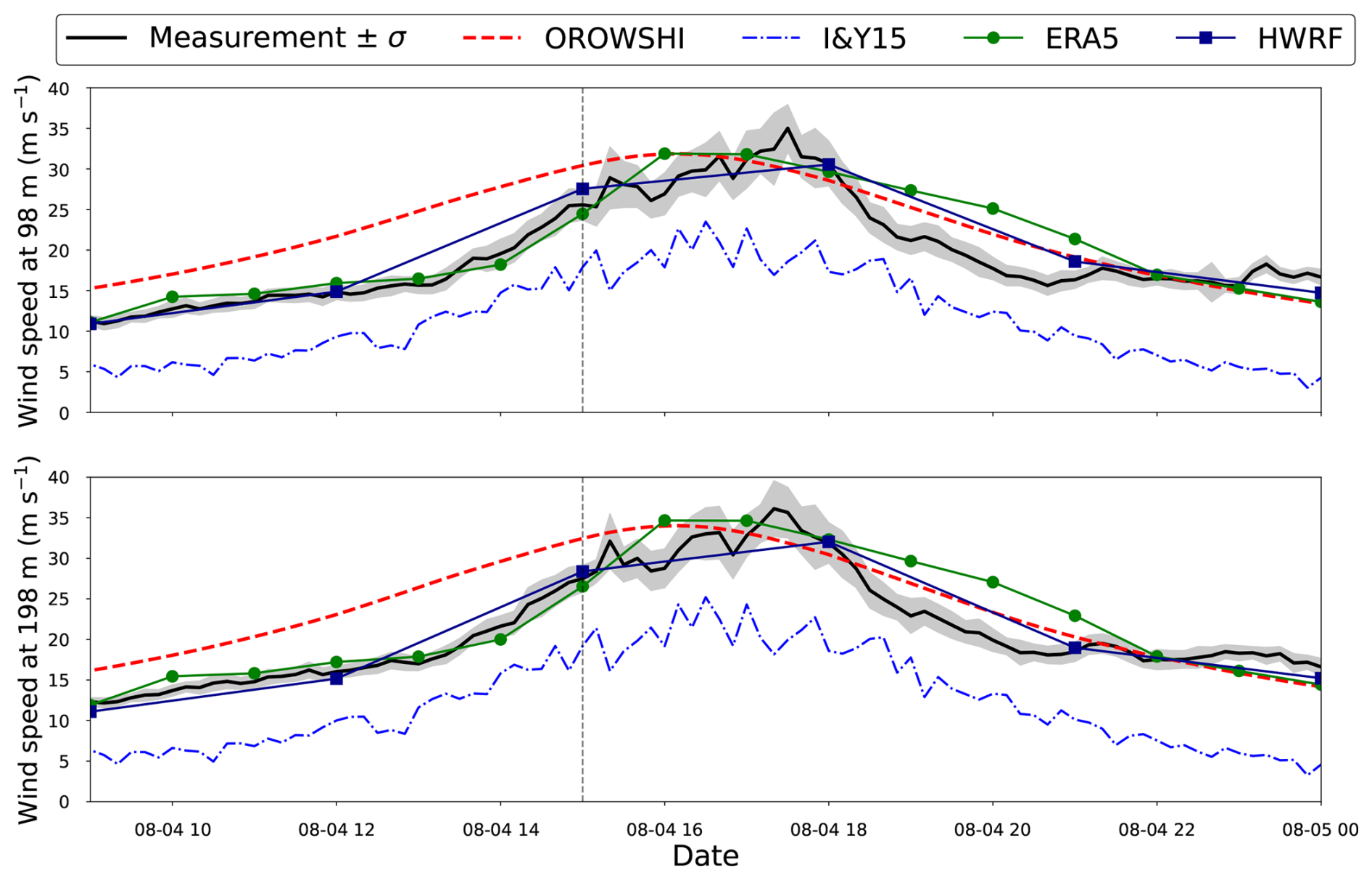
Figure 13 Time series of observed and predicted winds of TC Isaias at 98 m (top panel) and 198 m (bottom panel). The vertical dashed line corresponds to the instant at which the surface wind field is assessed.

Figure 14 shows the surface wind field of Isaias on 8 August at 15:00 GMT, at the HWRF time step closest to the maximum observed wind speed, when part of the TC is over open-ocean. The TC made landfall at the shown time step. The high-wind area is above the ocean according to HWRF. The faster decay of the wind speed profile with increasing distance to the TC centre using the I&Y15 model causes the TC to have reduced coverage, that is, smaller area of high wind speeds larger than 20 m s⁻¹, than the other methods, which explains the wind speed underestimation at the measurement site, being ≈220 km to the north-west of the cyclone centre at the shown time. Note that the I&Y15 model takes into account the ambient pressure, set to 1013 hPa here. A more accurate estimate of this pressure would lead to different results.

6.4 Typhoon Dujuan (2015) and Megi (2016)

Wind speeds in Taiwan are presented in Figs. 15–17. The parametric models can reproduce the increase in the wind until the main peak but deviate from the measurement during the leaving phase, with large discrepancies during low-wind conditions.

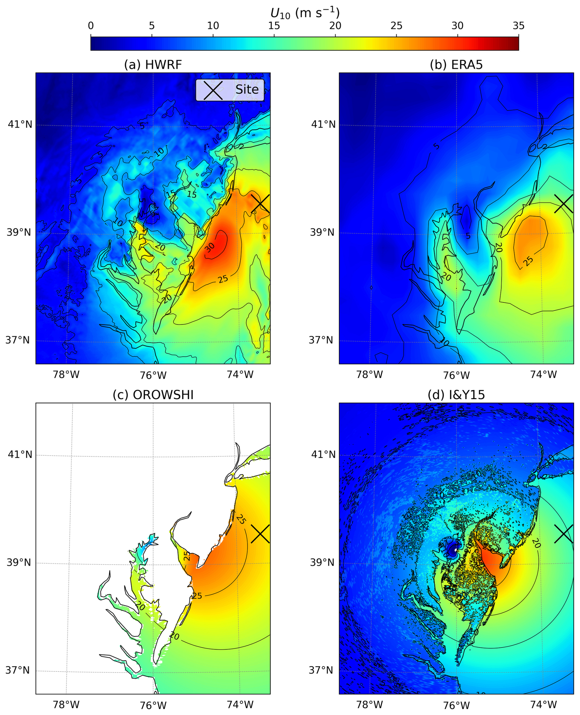
Figure 14 TC Isaias surface wind field on 8 August at 15:00 GMT predicted by HWRF (a), ERA5 (b), OROWSHI wind model (c), and I&Y15 wind model (d).

Figure 15 Time series of observed and predicted winds of TC Dujuan at 90 m (site 1).

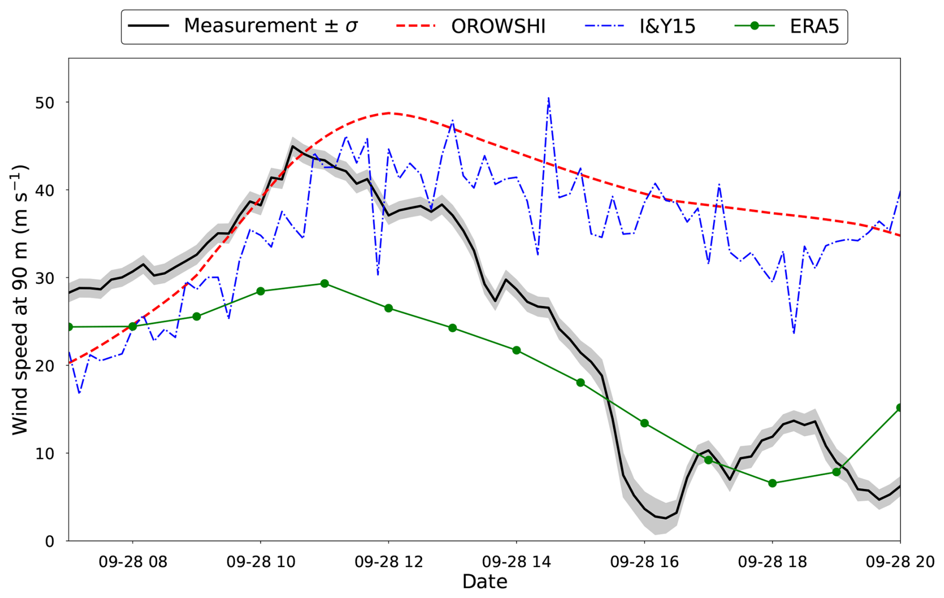
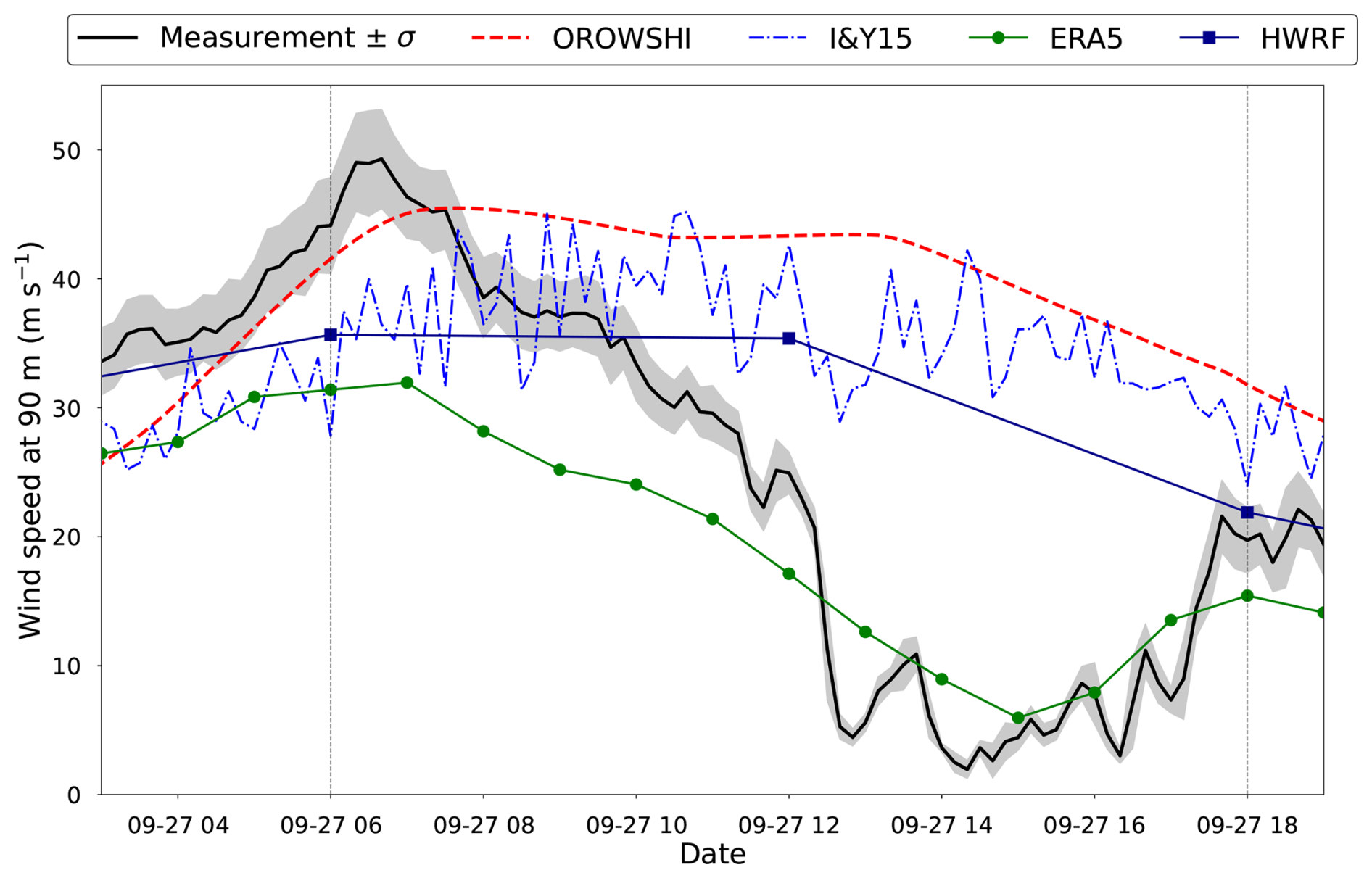
Figure 16 Time series of observed and predicted winds of TC Megi at 90 m (site 1). The vertical dashed lines correspond to the instants at which the surface wind field is assessed.

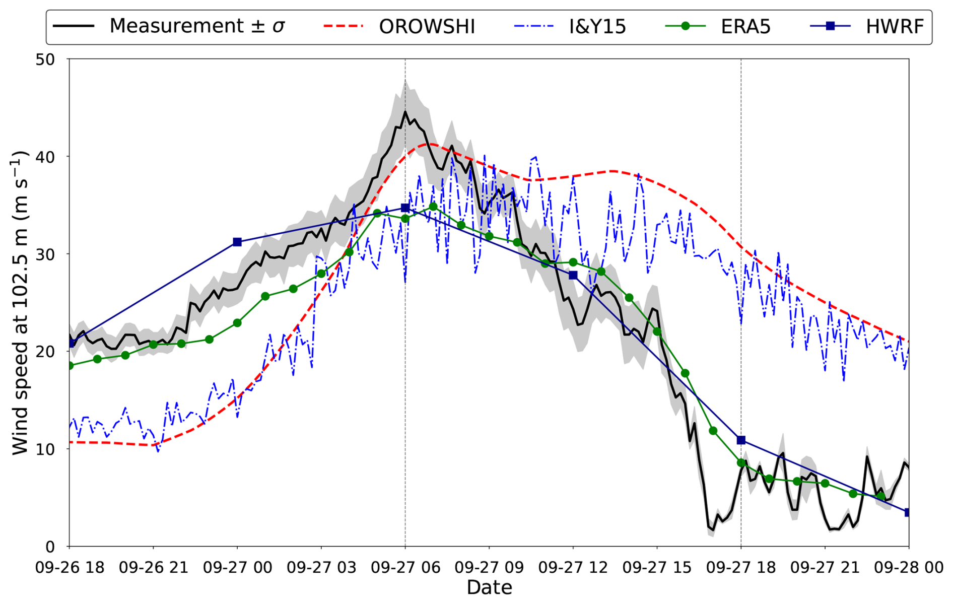
Figure 17 Time series of observed and predicted winds of TC Megi at 102.5 m (site 2). The vertical dashed lines correspond to the instants at which the surface wind field is assessed.

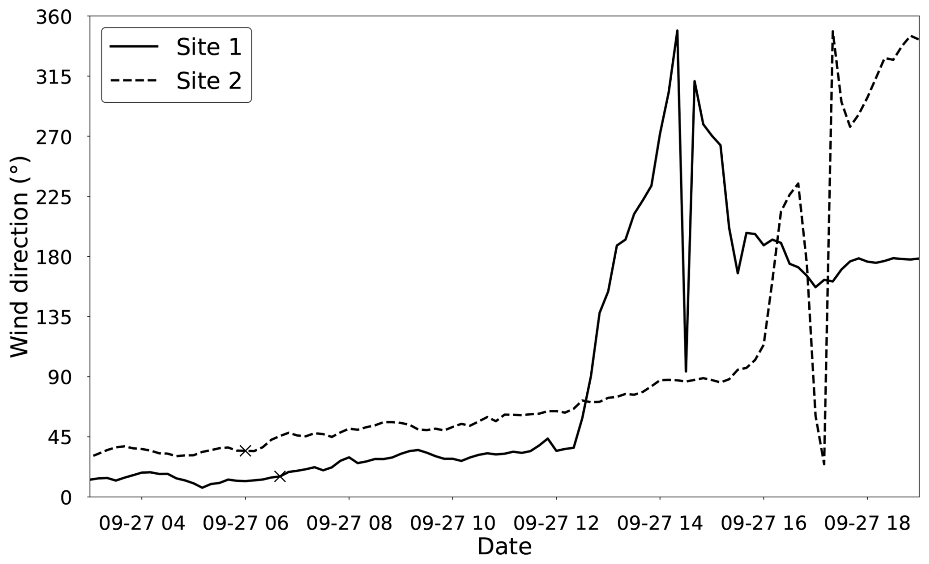
Figure 18 Time series of wind direction during TC Megi at sites 1 and 2. The crosses correspond to the instants of maximum wind speed measured on the measurement sites.

The wind direction measured by the wind vanes during TC Megi is presented in Fig. 18. The crosses correspond to the instant of maximum wind speed measured at sites 1 and 2. The wind blows from the sea during the main peak (wind direction lower than 30° for site 1 and 70° for site 2). Therefore, neglecting orographic effects has no impact on the maximum speed estimate in this specific case. Thus, the parametric models captured the main peak fairly well with a relatively low |PD_max| (less than 13 %); see Tables 8–10) compared to the results from HWRF and ERA5. Indeed, HWRF and ERA5 highly underestimate the maximum wind speeds in these cases with |PD_max| larger than 20 %, although both models account for the presence of the island. The wind decreases significantly after the main peak as the TC moves to the Taiwan Strait, and the blockage effect due to the island highly affects the wind prediction.

Table 8 Scores of the wind models for TC Dujuan at 90 m (site 1).

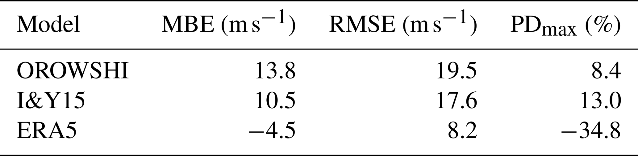
Table 9 Scores of the wind models for TC Megi at 90 m (site 1).

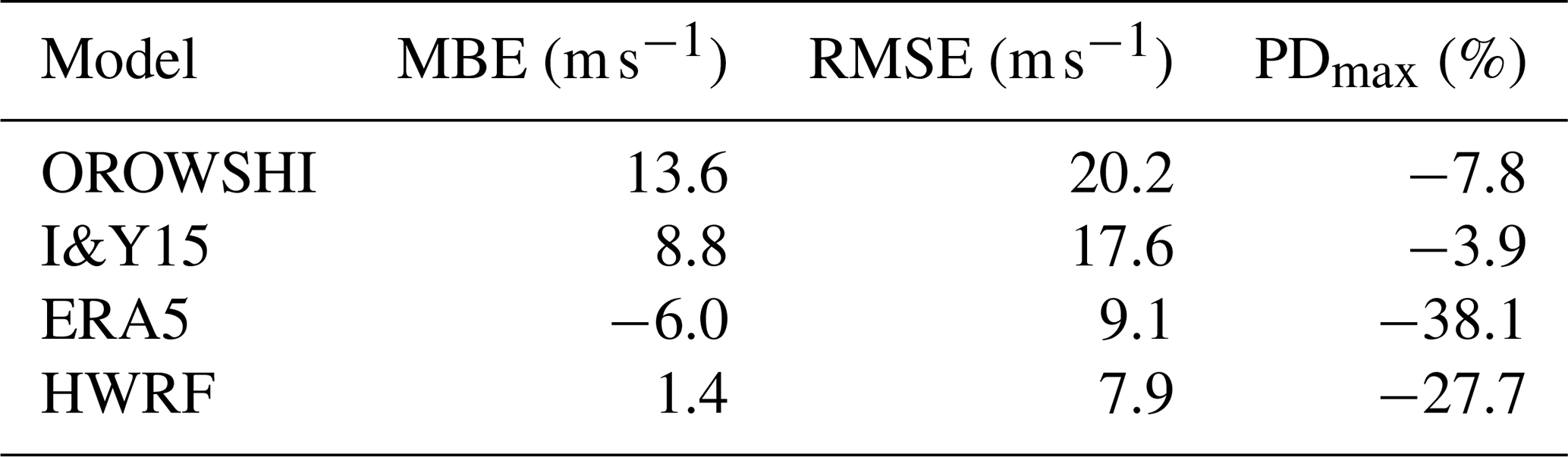
Table 10 Scores of the wind models for TC Megi at 102.5 m (site 2).

As HWRF results are not available for Typhoon Dujuan, the surface wind assessment focuses on Typhoon Megi, which was also studied in Müller et al. (2024a, b) among two similar configurations. The surface wind field of TC Megi on 27 September at 06:00 GMT is shown in Fig. 19. This time step corresponds to the time instant of maximum speed measured at site 2 and is also selected to illustrate the complexity of the interaction with Taiwan. The wind field predicted by HWRF (Fig. 19a) is highly unstructured, while ERA5 (Fig. 19b) largely underestimates the surface wind around the island. Also, at site 1, the wind speed at the second altitude (222 m) predicted by HWRF is slightly lower than the surface wind, leading to a negative shear exponent at this instant ($-\mathrm{2.8}\times {\mathrm{10}}^{-\mathrm{3}}$). The vertical extrapolation using a power law is thus invalid between the first two levels, while the wind speed increases for the vertical levels above several hundred metres. ERA5, on the other hand, predicts a shear exponent of 0.173 at the same instant but highly underestimates the observed wind speeds.

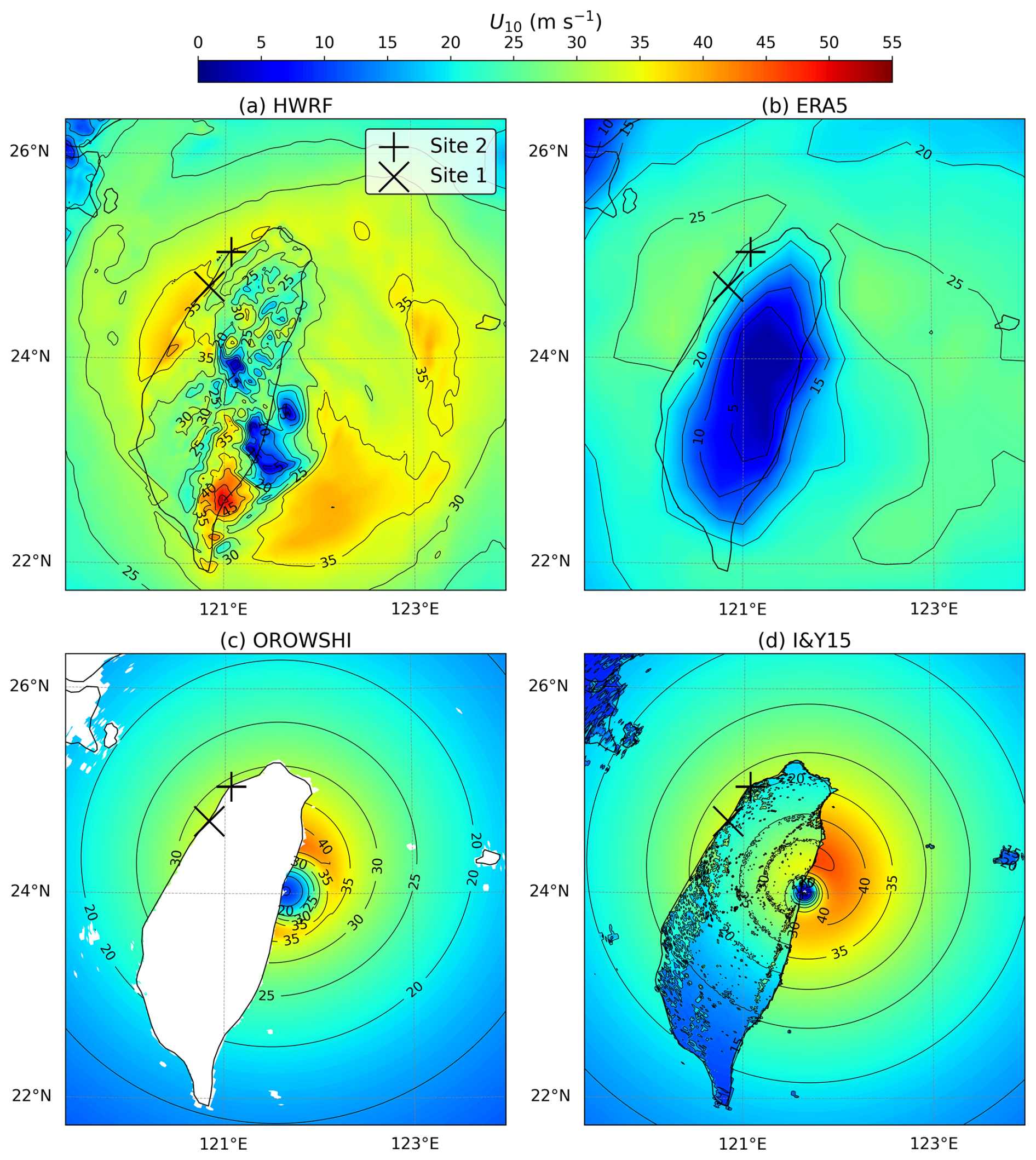
Figure 19 TC Megi surface wind field on 27 September at 06:00 GMT predicted by HWRF (a), ERA5 (b), OROWSHI wind model (c), and I&Y15 wind model (d).

Due to the presence of the mountains, the eyewalls predicted by both the OROWSHI model (Fig. 19c) and I&Y15 (Fig. 19d) are unrealistic as the parametric models do not account for the asymmetry caused by the orography here. An eyewall positioned on the opposite side of the obstacle (i.e. in the south-eastern quadrant) would be more consistent with HWRF results. Nevertheless, the wind speed in the outer core is fairly predicted and the magnitude of wind speed is reasonably estimated at this instant (see Figs. 16 and 17). HWRF predicts the highest intensity among the models. However, the highest wind in Fig. 19a might be due to orographic acceleration over the island (south part of Taiwan).

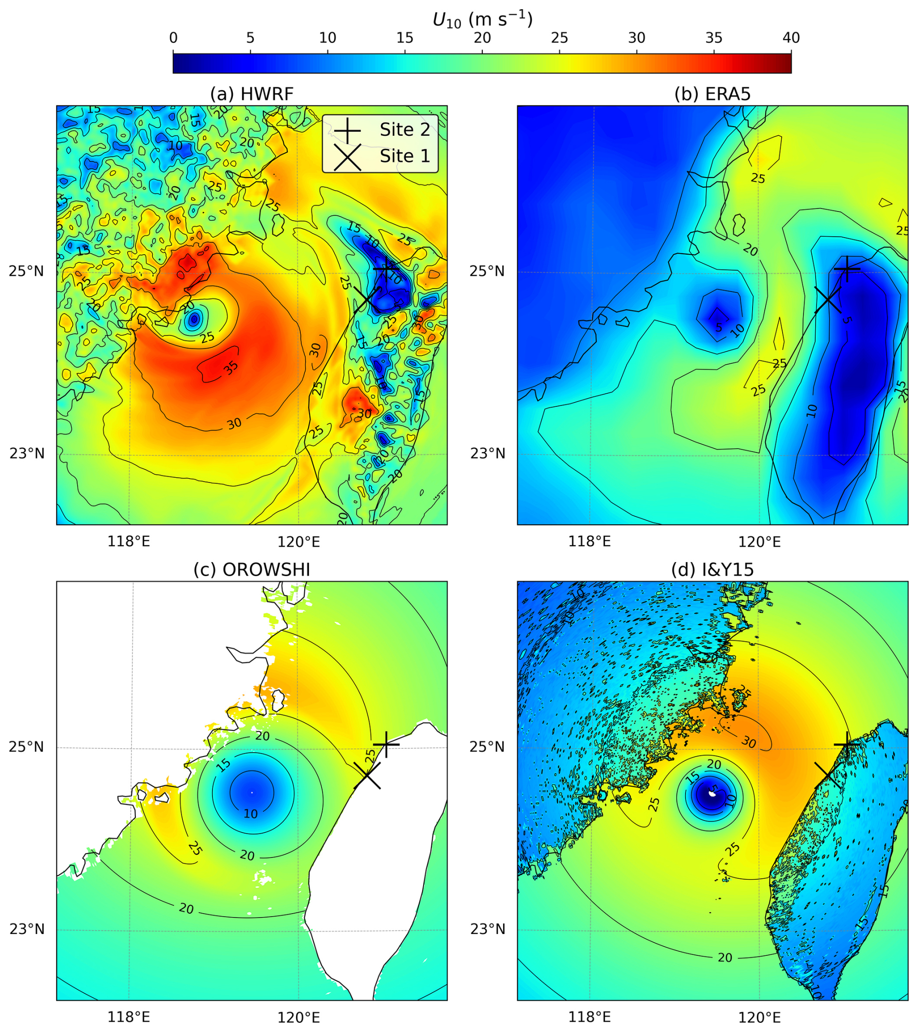
Figure 20 TC Megi surface wind field on 27 September at 18:00 GMT predicted by HWRF (a), ERA5 (b), OROWSHI wind model (c), and I&Y15 wind model (d).

When the TC passes through the Taiwan Strait, the wind direction increases as the TC propagates westward, with the sites located to the north of the cyclone track (Fig. 18), and the wind speed decreases significantly (Figs. 16 and 17). The measurement zone becomes very calm with low wind speeds due to the mountain blockage. This is also reported in Müller et al. (2024b), where wind shear and veer vary highly in this area. Large variations in wind direction occur at low wind speeds (see Figs. 16–18). Parametric models largely overestimate wind at these instants by neglecting orography effects. Thus, the RMSE for the two parametric models are much higher than in the other configurations (RMSE>12 m s⁻¹; see Tables 8–10). HWRF and ERA5 can predict this phenomenon better as they incorporate the influence of the terrain. This is illustrated in Fig. 20, where the wind field of the four models is displayed for TC Megi on 27 August at 18:00 GMT. At this time, the TC is located in the Taiwan Strait, and complex interactions occur with the island. HWRF can capture fine features due to its high resolution, including orographic acceleration and deceleration, both on the continent and on Taiwan. However, the most interesting pattern is the wake effect north-west of the island at the site locations, caused by the upstream mountainous terrain that strongly disturbs the wind flow. This is also predicted by ERA5 despite its coarse resolution (Fig. 20b). Also, both ERA5 and HWRF predict an area of strong winds located over the sea at this instant, located in the direction opposite to the TC translation (299° at this time). The region of highest wind speeds is confined between the two obstacles, Taiwan and the continental shelf. This illustrates the complexity of wind forecasting using simplified parametric models that do not account for large-scale disturbances generated by an island like Taiwan.

Table 11 Mean absolute scores of the wind models.

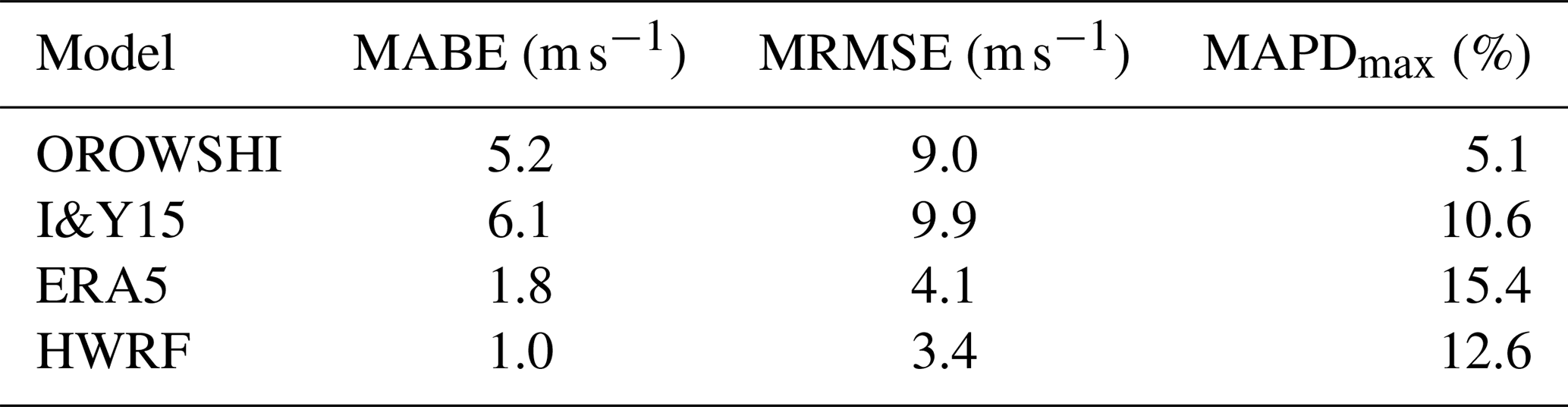
6.5 Synthesis

The mean absolute bias error (MABE), the mean root mean square error (MRMSE) on the wind time series, and the mean absolute percentage deviation from the maximum measured wind (MAPD_max) are presented in Table 11.The whole time series is better predicted by the reanalysis and the mesoscale model ($\text{MABE}<\mathrm{2}\mathrm{m}{\mathrm{s}}^{-\mathrm{1}}$ and $\text{MRMSE}<\mathrm{4}\mathrm{m}{\mathrm{s}}^{-\mathrm{1}}$) than by the parametric models, which show larger errors ($\text{MABE}\gg \mathrm{5}\mathrm{m}{\mathrm{s}}^{-\mathrm{1}}$ and $\text{MRMSE}>\mathrm{9}\mathrm{m}{\mathrm{s}}^{-\mathrm{1}}$). These deviations are essentially caused by the overestimation of the wind speeds during the passage of the TCs through the Taiwan Strait and the significantly underestimation of wind speeds of Isaias by the I&Y15 model. On the other hand, the parametric models better estimate the highest wind at the sites, an essential parameter for extreme wind statistics. In particular, the OROWSHI model shows only a 5.1 % mean absolute percent deviation from the peak observed wind speed, which is less than half the error of the other methods. ERA5 largely underestimates the peak winds, and should therefore be used with caution for tropical cyclone wind assessment. The parametric models are highly effective in their field of application, i.e. on the open-ocean without large-scale disturbances. The source of errors in parametric models is mainly due to land interactions that affect the TC asymmetry and orographic effects that strongly decrease wind speed downstream of Taiwan's mountains. In complex environments where tropical cyclones are perturbed at the mesoscale, advanced numerical models are required to capture complex flows. Coupling the ERA5 wind field with a TC parametric model also appears to be a viable approach for improving wind speed predictions under such conditions, as demonstrated by Liu et al. (2025).

7 Conclusions

Tropical cyclone risk assessment mainly relies on the statistical generation of synthetic events to which a parametric wind model is applied. In offshore wind turbine design, the wind speed is extrapolated at hub height. To keep production costs down, and to avoid overly conservative designs due to the uncertainty associated with the lack of knowledge of this extreme phenomenon, reliable and accurate simulation models are essential. This paper is dedicated to the modelling of extreme wind speed in TCs using simplified parametric models that are compared with measurements at relevant altitudes for the offshore wind industry. The model introduced here is based on a surface wind field calibrated on SAR measurements. The wind is vertically extrapolated using a logarithmic law and the WASP drag coefficient. Parameters from the US agency are used, allowing the model to be applied to any basin. In some cases, local orographic effects are accounted for by using a numerical speed-up ratio. The main aim of this research is to assess the performance of this parametric model at specific sites impacted by tropical cyclones by comparing the wind time series with in situ observations on one hand and with more advanced numerical models on the other hand.

Wind measurements of five TC events are analysed to evaluate the performance of the WASP formulation to estimate wind speeds at altitude from surface winds. The drag coefficients obtained from the measurements are scattered but the mean value is consistent with the proposed formulation. This parameterisation enables efficient wind prediction at hub height and is more accurate than that recommended in the design standards for this dataset. The power law is also assessed as an alternative, the mean value derived from the measurement is 0.106.

Furthermore, modelled time series of wind speeds are compared with measurements and results from HWRF and ERA5. The wind model used in Ishihara and Yamaguchi (2015) is implemented for comparison. In general, the two parametric formulations perform as well as the reanalysis and the mesoscale model and show a fair agreement with the measurement given the simplicity and the computational cost of these models. Scores such as MBE, RMSE, and percent deviation on the maximum wind are computed for each event. In a design context where estimating the maximum wind speed is essential, the parametric models are more accurate than HWRF and ERA5. In particular, the OROWSHI model presents only a 5.1 % PD_max from the maximum observed wind at sites, over twice as accurate as the other approaches. For its ease of implementation, computational cost, and most importantly its ability to accurately predict the most severe winds induced by tropical cyclones, the model is suitable for implementation within a Monte Carlo framework to derive extreme wind statistics. Also, the surface wind fields are compared to discuss and analyse the differences between the models. The I&Y15 surface wind generally presents a broader eyewall than the OROWSHI model and HWRF results, which could lead to significant differences in terms of wave height estimates as wave models are forced with surface winds. The assessment of wind fields near large obstacles reveals the main limitation of the parametric models. These models, originally designed to represent tropical cyclones under ideal conditions, i.e. intense and over open-ocean, tend to exhibit their largest errors when the cyclone deviates from this configuration. Landfalling TCs experience strong orographic effects that displace or attenuate wind maxima, leading to significant discrepancies with in situ observations, as seen near Ky$\overline{\text{u}}$sh$\overline{\text{u}}$ Island and Taiwan (Nanmadol, Megi). The magnitude of this landfall effect depends on coastline geometry and TC track. When the storm interacts with large obstacles, errors increase, particularly at sites exposed to offshore winds, already affected by land. Using parametric models instead of advanced dynamical models is therefore problematic for site-specific studies in regions with pronounced coastal orography. A minimal improvement would involve a site-adapted and more advanced parameterisation of asymmetry, accounting for variations in amplitude and azimuthal location based on the statistical properties at each site of interest. Finally, a more detailed analysis of wind direction variability and turbulence characteristics will be carried out in future work, based on the available dataset, to further improve the representation of tropical cyclone wind fields for wind energy applications.