A consistent computational fluid dynamics surrogate model for wind turbine interaction including atmospheric stability

Wind turbine wake and blockage effects can reduce the energy yield in wind farms, and fast models are required to mitigate these effects by wind farm layout optimization. However, most fast models do not account for important physics that impact wake and blockage effects, as for example atmospheric stability. In this work, we propose a surrogate model of a Reynolds-averaged Navier–Stokes (RANS) wind farm model including atmospheric surface layer stability that is about 5 orders of magnitude faster than the original model. The surrogate model is based on a single-wake database of stream-wise velocity deficit and wake-added turbulence intensity, generated by a RANS model. The surrogate model is evaluated against the RANS model for different inflow conditions and wind farms. The errors in the surrogate model are reduced by a factor of 2 to 4 when taking into account wake-added turbulence intensity and the use of a rotor-averaging model in combination with a momentum-based wake superposition method. The latter leads to a more consistent surrogate model compared to using linear superposition without a rotor-averaging model. However, the computational effort of the surrogate model is still an order of magnitude larger compared to traditional engineering wake models, and more research is required to reduce it.

1 Introduction

Interaction of wind turbines and wind farms can lead to energy losses (Barthelmie et al., 2007) mainly due to wake and blockage effects (Bleeg et al., 2018). These losses can be minimized by optimizing a wind farm layout, which requires fast wake models, commonly known as engineering wake models. However, such models often rely on strong assumptions of the wake shape (Jensen, 1983; Bastankhah and Porté-Agel, 2014) and wake superposition model (Katic et al., 1987) and rarely take into account important effects of the atmospheric boundary layer (ABL), such as atmospheric stability; Coriolis forces; and turbine-related effects, including the thrust force distribution and wake rotation. High-fidelity wake models based on computational fluid dynamics (CFD) can include such effects but are too expensive for the application of wind farm layout optimization. A common approach is to use high-fidelity model results as training data for engineering wake models. This ranges from a simple calibration of an engineering wake model constant (Niayifar and Porté-Agel, 2016; Peña et al., 2016) up to complex surrogate modeling for both steady-state (Schulte and Stoevesandt, 2014) and dynamic wake models (Andersen and Murcia Leon, 2022). A more detailed review of low- and high-fidelity wake models can be found in Göçmen et al. (2016); Porté-Agel et al. (2020). In addition, Porté-Agel et al. (2020) also reviewed the effect of different atmospheric conditions on wind turbine wakes, characterized by ambient turbulence intensity and atmospheric stability.

Steady-state models based on Reynolds-averaged Navier–Stokes (RANS) can be used to calculate the mean flow of a wind turbine in isolation, from which a wind farm flow can be constructed using a superposition model. This model type can be considered to be a surrogate model that solves the RANS equations for an entire wind farm (Prospathopoulos et al., 2011; van der Laan et al., 2015b). An overview of existing RANS-based surrogate models can be found in Table 1. The lowest model fidelity listed in Table 1 is based on a linearized set of RANS equations, where the effects of the thrust force are added as a linear perturbation to a base flow (Ott et al., 2011; Ebenhoch et al., 2017), and a wind farm flow is constructed by linear superposition of a single-wake shape multiplied by the thrust coefficient, C_T. Fuga (Ott et al., 2011) is a linearized RANS model where the base flow represents the atmospheric surface layer, including atmospheric stability following Monin–Obukhov similarity theory (MOST) (Monin and Obukhov, 1954). Ebenhoch et al. (2017) argued that the wake velocity deficit is only a linear function of the thrust coefficient for C_T<0.5 using 1D momentum theory. However, RANS single-turbine simulations show that the effect of the thrust coefficient is nonlinear even for low thrust coefficients, e.g., C_T=0.1, because the wake recovery increases with C_T, as shown in Appendix A. A higher C_T leads to larger velocity gradients that reduce the downstream extent of the near-wake, as shown by LES results of Sørensen et al. (2015). Schulte and Stoevesandt (2014) developed a surrogate model of (nonlinear) RANS simulations where the turbine is modeled as an actuator disk (AD) (Mikkelsen, 2003). A database of single-wake velocity deficits was pre-calculated and stored as a lookup table (LUT) for a range of wind speeds using RANS-AD simulations, and a wind farm flow was created by superposition. Jacquet et al. (2022) developed a similar RANS surrogate model for simulating wind farm blockage but also included effects of atmospheric stability following MOST. The Fuga and the RANS-LUT models of Schulte and Stoevesandt (2014) and Jacquet et al. (2022) do not take wake-added turbulence intensity (TI) into account. Criado Risco et al. (2023) followed a similar approach to Schulte and Stoevesandt (2014) and Jacquet et al. (2022) but extended the RANS-LUT model by including both shapes of velocity deficits and wake-added TI that depend on the thrust coefficient and ambient turbulence intensity. A wind farm flow was constructed by superposing the velocity deficit and wake-added TI, looking up different wake shapes for the local TI and thrust coefficient obtained from the local wind speed; the best results were obtained for linear superposition. Criado Risco et al. (2023) developed the RANS-LUT model for neutral surface layer conditions and verified the flow field of the RANS-LUT model for neutral conditions against RANS-AD wind turbine row simulations.

(Ott et al., 2011)(Schulte and Stoevesandt, 2014)(Jacquet et al., 2022)(Criado Risco et al., 2023)

Table 1 RANS-based surrogate wake models: LUT flow variables and input dimensions.

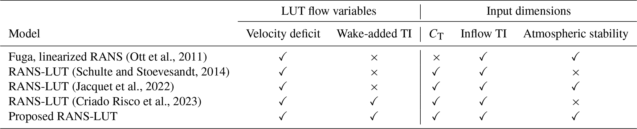
In this work, we extend the model of Criado Risco et al. (2023) by including atmospheric stability following MOST, and we compare the results with full RANS-AD wind farm simulations, including wind turbine power, for a range of stability conditions following MOST. In addition, an alternative superposition method is applied to the velocity field, which is based on the momentum-conserving superposition method of Zong and Porté-Agel (2020). The latter leads to a more consistent model that can be used to obtain good results of both the wind farm flow and turbine power. Finally, we show the importance of including wake-added TI in the RANS-LUT model. The proposed RANS-based surrogate model is summarized in Table 1. The RANS-AD and extended RANS-LUT models are described in Sect. 2, and the results are discussed in Sect. 3.

2 Methodology

The proposed RANS-LUT surrogate model is based on a database of single-wake simulations. In this work, RANS-AD simulations are employed to generate the aforementioned database and are discussed in detail in Sect. 2.2. The RANS-AD model is also used to run a set of wind farm simulation test cases, discussed in Sect. 2.1, to evaluate the performance of the RANS-LUT model. The original RANS-LUT model of Criado Risco et al. (2023) for the neutral case and proposed extensions are discussed in Sect. 2.3.

2.1 Test cases

The RANS-LUT model results are evaluated against RANS-AD simulations of a row of regularly spaced wind turbines and a square regular wind farm layout consisting of 1×8 and 8×8 turbines, respectively. The turbine row is simulated for a row-aligned wind direction, while the square wind farm is simulated for a range of wind directions for every 3° between 270 and 315°, where 270 and 315° are aligned with a wind farm edge and a wind farm diagonal, respectively. The test cases are listed in Table 2. Each case is simulated for a turbine spacing of 4D and 8D, with D as the rotor diameter, and two inflow wind speeds corresponding to a below- and above-rated wind speed, which lead to different thrust coefficients. Furthermore, three different stability conditions, labeled as stable, neutral, and unstable, are employed that differ in both ambient TI and surface layer stability. Here, the TI is based on the turbulent kinetic energy at hub height, and the stability parameter is defined as ${\mathit{\zeta }}_{\text{ref}}=(z_{\text{ref}}+z_{\mathrm{0}})/L$, with z_ref as the reference height set equal to the hub height, z₀ as the roughness length, and L as the Obukhov length. The TI and ζ_ref values are $\mathit{\{}\mathrm{0.05},\mathrm{0.06},\mathrm{0.1}\mathit{\}}$ and $\mathit{\{}\mathrm{0.5},\mathrm{0},-\mathrm{0.5}\mathit{\}}$ for the stable, neutral, and unstable cases, respectively. The resulting normalized profiles are shown in Fig. 1 and further discussed in Sect. 2.2.

Table 2 Test cases.

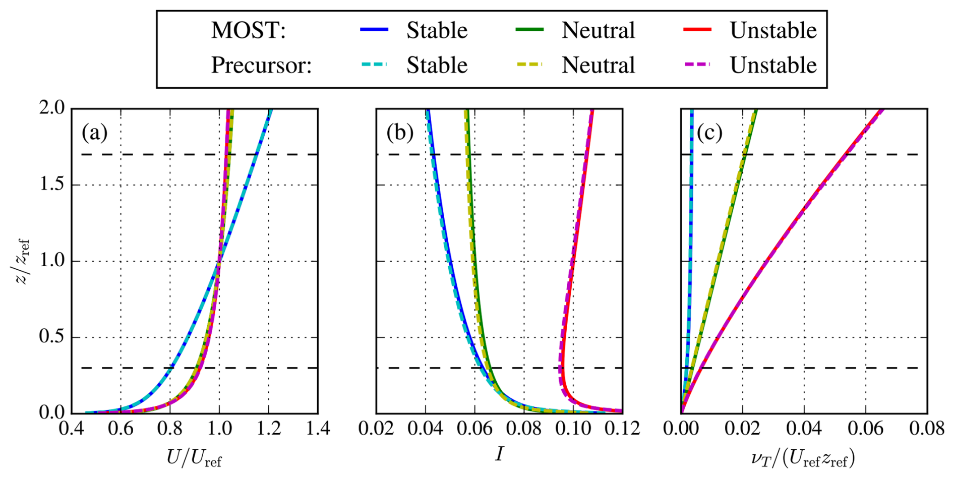
Figure 1 Normalized inflow profiles of wind speed (a), turbulence intensity (b), and eddy viscosity (c) as computed by the 1D precursor and compared with MOST. Rotor area of the NREL-5 MW reference turbine is depicted with horizontal dashed lines.

The employed turbine is based on the NREL-5MW reference turbine (Jonkman et al., 2009), which has a rotor diameter and hub height of 126 and 90 m, respectively. However, we use a general turbine model to represent the wind speed curves of the thrust coefficient C_T(U), the power coefficient C_P(U), and the tip speed ratio λ(U), with constant below-rated values of C_T,r=0.8, C_P,r=0.45, and λ_r=7.5 (van der Laan et al., 2022), leading to a rated wind speed U_r of 11.33 m s⁻¹. The use of a general turbine model makes it easier to test the RANS-LUT surrogate model against RANS-AD simulations of wind farms using a constant C_T and variable C_T by applying below- and above-rated wind speed cases, as listed in Table 2. The generic turbine model is fully defined as (van der Laan et al., 2022)

$$\begin{array}{}\text{(1)}& \begin{array}{rl}{\displaystyle }{U}_{\text{in}}\le U\le U_{\text{r}}:& {\displaystyle }{C}_{\mathrm{T}}=C_{\text{T,r}},C_{\mathrm{P}}=C_{\text{P,r}},\mathit{\lambda }={\mathit{\lambda }}_{\mathrm{r}},\\ {\displaystyle }{U}_{\text{r}}<U\le U_{\text{out}}:& {\displaystyle }{C}_{\mathrm{T}}=C_{\text{T,r}}(U_{\mathrm{r}}/U{)}^{\mathrm{3.2}},\\ {\displaystyle }& {\displaystyle }{C}_{\mathrm{P}}=C_{\text{P,r}}(U_{\mathrm{r}}/U{)}^{\mathrm{3}},\mathit{\lambda }={\mathit{\lambda }}_{\mathrm{r}}(U_{\mathrm{r}}/U),,\end{array}\end{array}$$

with $U_{\text{in}}=\mathrm{4}\mathrm{m}{\mathrm{s}}^{-\mathrm{1}}$ and $U_{\text{out}}=\mathrm{25}\mathrm{m}{\mathrm{s}}^{-\mathrm{1}}$ as the cut-in and cut-out wind speed, respectively. The above-rated thrust coefficient follows a power law with exponent 3.2, which fits turbine data well, covering a large range of turbine sizes (van der Laan et al., 2022).

2.2 RANS-AD CFD model

The RANS-AD simulations are conducted with the CFD wind farm flow framework PyWakeEllipSys v5.4 (DTU Wind and Energy Systems, 2025), which uses the in-house incompressible finite-volume CFD solver EllipSys3D, initially developed by Michelsen (1992) and Sørensen (1994). The AD model (Réthoré et al., 2014; Troldborg et al., 2015) is based on a polar grid using 10 and 32 cells in the radial and azimuthal directions, respectively. Thrust and tangential force distributions are calculated with the analytical model of Sørensen et al. (2020), which depends on C_T, C_P, and λ. The force distributions are scaled with the local shear while maintaining the input integral forces (van der Laan et al., 2020).

2.2.1 Numerical domain

The numerical grid is a Cartesian domain with a refined region around the horizontal center at which the turbines are placed. The grid topology and boundary conditions are the same as specified in van der Laan et al. (2024); however, the domain dimensions are case-specific. For the single-wind-turbine case, a domain with dimensions $\mathrm{1024}D\times \mathrm{1005}D\times \mathrm{25}D$ is employed for the streamwise, lateral, and vertical directions, respectively. The inner refined domain is employed to resolve the wind turbine wake(s). It has dimensions $\mathrm{24}D\times \mathrm{5}D\times \mathrm{3}D$, is placed at $\mathrm{4}\le x/D\le \mathrm{20}$ and $\mathrm{2.5}\le y/D\le \mathrm{2},\mathrm{5}$, and contains a mesh with uniform horizontal spacing of $D/\mathrm{8}$. Vertically, the cells grow with height up to $D/\mathrm{8}$ in the rotor area and $D/\mathrm{6}$ at the end of the refined domain using a first cell height of $D/\mathrm{200}$. The cells are distributed as $\mathrm{288}\times \mathrm{128}\times \mathrm{64}$, leading to a total number of 2.4 million cells. The cell spacing of $D/\mathrm{8}$ is sufficient to resolve the wind farm flow under neutral conditions (van der Laan et al., 2015c). A finer grid spacing may be necessary for stable-inflow cases depending on the user's quantity of interest. For the present study, we use the same grid spacing of $D/\mathrm{8}$ for all stability cases for simplicity. Our goal is to evaluate the RANS-LUT surrogate model against RANS-AD wind farm simulations using the same grid spacing. If one would like to apply a finer spacing, then the refined single-wake database would also improve the RANS-LUT model. A grid refinement study of RANS-AD single-wake simulations is performed in Appendix C. The numerical domains of the wind turbine row and square wind farm are larger in the horizontal extent, and the corresponding grid dimensions are listed in Table 3.

Table 3 Domain dimensions and number of cells of RANS-AD single-wake and wind farm test cases.

2.2.2 Inflow and turbulence model

The inflow conditions represent an atmospheric surface layer including atmospheric stability following MOST (Monin and Obukhov, 1954). We employ a two-equation k–ε turbulence model that is in balance with MOST (van der Laan et al., 2017; Doubrawa et al., 2020; Baungaard et al., 2022a), which is important for isolating the turbine and wind farm flow effects. The turbulence model has the following form:

$$\begin{array}{}\text{(2)}& {\displaystyle }& {\displaystyle }{\mathit{\nu }}_{\mathrm{T}}=C_{\mathit{\mu }}{f}_{\mathrm{P}}(\mathit{\sigma }/\stackrel{\mathrm{̃}}{\mathit{\sigma }},C_{\mathrm{R}},C_{\mathrm{B}}){\displaystyle \frac{k^{\mathrm{2}}}{\mathit{\epsilon }}},\text{(3)}& {\displaystyle }& {\displaystyle \frac{Dk}{Dt}}={\displaystyle \frac{\partial }{\partial x_j}}\left[\left(\mathit{\nu }+{\displaystyle \frac{{\mathit{\nu }}_{\mathrm{T}}}{{\mathit{\sigma }}_k}}\right){\displaystyle \frac{\partial k}{\partial x_j}}\right]+\mathcal{P}+\mathcal{B}-\mathit{\epsilon }+S_k,\text{(4)}& {\displaystyle }& {\displaystyle }\begin{array}{rl}{\displaystyle \frac{D\mathit{\epsilon }}{Dt}}=& {\displaystyle \frac{\partial }{\partial x_j}}\left[\left(\mathit{\nu }+{\displaystyle \frac{{\mathit{\nu }}_{\mathrm{T}}}{{\mathit{\sigma }}_{\mathit{\epsilon }}}}\right){\displaystyle \frac{\partial \mathit{\epsilon }}{\partial x_j}}\right]\\ {\displaystyle }& {\displaystyle }+(C_{\mathit{\epsilon },\mathrm{1}}\mathcal{P}-C_{\mathit{\epsilon },\mathrm{2}}\mathit{\epsilon }+C_{\mathit{\epsilon },\mathrm{3}}\mathcal{B}){\displaystyle \frac{\mathit{\epsilon }}{k}},\end{array}\end{array}$$

with $x_j=\mathit{\{}x,y,z\mathit{\}}$ as the Cartesian coordinates in streamwise, lateral, and vertical directions, respectively. The turbulence model solves equations for the turbulent kinetic energy, k, and its dissipation, ε, from which the eddy viscosity, ν_T, is calculated. In addition, the Boussinesq hypothesis (Boussinesq, 1897) is applied to compute the Reynolds stresses. The source terms 𝒫 and ℬ represent the production of turbulence due to shear and buoyancy, respectively; the latter is negative for stable conditions. The effect of the non-neutral conditions is mainly modeled by the turbulent buoyancy source term since a momentum buoyancy source and a temperature equation are not employed. The MOST profiles are in balance with the turbulence model using an additional source term S_k and a height-dependent C_ε,3 (van der Laan et al., 2017). They are derived by substituting the MOST similarity functions of the normalized shear and potential temperature gradient into the k−ε turbulence model; the full expressions of S_k and C_ε,3 are provided in van der Laan et al. (2017). The original turbulence model used a buoyancy source that was a function of the stability and local shear. However, this can lead to a non-physical wake recovery for unstable conditions, where an increase in turbulent buoyancy production could lead to less wake recovery. In the present work, we use a constant turbulent buoyancy source term, $\mathcal{B}=u_{*}^{\mathrm{3}}/\left(\mathit{\kappa }L\right)$, which solves the wake recovery problem for unstable conditions (Baungaard et al., 2022a). Here, u_* is the friction velocity, and κ=0.4 is the von Kármán constant. However, we find that using a constant buoyancy source term for stable conditions can lead to numerical instabilities. For stable conditions, the constant buoyancy source is negative and reduces k. When the k equation is solved for, the other source terms can vary, while the buoyancy source remains constant. This can lead to negative k values. The numerical problem is solved by multiplying the constant buoyancy source term by the ratio of local eddy viscosity, ν_T, to inflow eddy viscosity, ν_T,MOST, for stable conditions only:

$$\begin{array}{}\text{(5)}& {\displaystyle }\mathcal{B}={\displaystyle \frac{u_{*}^{\mathrm{3}}}{\mathit{\kappa }L}}{\displaystyle \frac{{\mathit{\nu }}_{\mathrm{T}}}{{\mathit{\nu }}_{T,\text{MOST}}}}={\displaystyle \frac{u_{*}^{\mathrm{3}}}{\mathit{\kappa }L}}{\displaystyle \frac{{\mathit{\nu }}_{\mathrm{T}}}{u_{*}\mathit{\kappa }z}}{\mathit{\varphi }}_{\mathrm{m}}\left(\mathit{\zeta }\right),\end{array}$$

with ϕ_m as the MOST function of normalized wind shear. The idea of using ${\mathit{\nu }}_{\mathrm{T}}/{\mathit{\nu }}_{T,\text{MOST}}$ in ℬ is based on the fact that both the original buoyancy production and the turbulent shear production also scale with ν_T. The modification does not change a single wake under stable conditions significantly. The eddy viscosity is limited with a near-wake-length-scale limiter, f_P (van der Laan et al., 2015c; van der Laan and Andersen, 2018), extended to non-neutral conditions (Doubrawa et al., 2020) and later revised for unstable conditions (Baungaard et al., 2022a). The f_P function depends on the local shear, $\mathit{\sigma }=k/\mathit{\epsilon }\sqrt{(\partial U_j/\partial x_j{)}^{\mathrm{2}}}$, normalized by the inflow shear, $\stackrel{\mathrm{̃}}{\mathit{\sigma }}=\mathrm{1}/\sqrt{C_{\mathit{\mu }}}\sqrt{{\mathit{\varphi }}_{\mathrm{m}}/{\mathit{\varphi }}_{\mathit{\epsilon }}}$, and two model constants, C_R=4.5 and C_B=5.0. The other constants in the turbulence model are set as $\mathit{\{}{C}_{\mathit{\mu }},{\mathit{\sigma }}_k,{\mathit{\sigma }}_{\mathit{\epsilon }},C_{\mathit{\epsilon },\mathrm{1}},C_{\mathit{\epsilon },\mathrm{2}}\mathit{\}}=\mathit{\{}\mathrm{0.03},\mathrm{1.0},\mathrm{1.3},\mathrm{1.21},\mathrm{1.92}\mathit{\}}$. Finally, the molecular viscosity, ν, is set as $\mathrm{1.78}\times {\mathrm{10}}^{-\mathrm{5}}{\mathrm{m}}^{\mathrm{2}}{\mathrm{s}}^{-\mathrm{1}}$ but has no influence on the solution since ν_T≫ν (van der Laan et al., 2020).

The non-dimensional inflow is defined by the TI based on the turbulent kinetic energy, $I_{\text{ref}}=\sqrt{\mathrm{2}/\mathrm{3}k}/U_{\text{ref}}$, and the stability parameter, ζ_ref, with U_ref as the freestream wind speed. I_ref and ζ_ref are used to set the roughness length, z₀, and the friction velocity, u_*:

$$\begin{array}{}\text{(6)}& \begin{array}{rl}{\displaystyle \frac{u_{*}}{U_{\text{ref}}}}& {\displaystyle }=f(I_{\text{ref}},{\mathit{\zeta }}_{\text{ref}})\\ {\displaystyle }& {\displaystyle }=I_{\text{ref}}\sqrt{\mathrm{3}/\mathrm{2}}{C}_{\mathit{\mu }}^{\frac{\mathrm{1}}{\mathrm{4}}}{\mathrm{\Phi }}_{\mathit{\epsilon }}\left({\mathit{\zeta }}_{\text{ref}}{)}^{-\frac{\mathrm{1}}{\mathrm{4}}}{\mathrm{\Phi }}_{\mathrm{m}}\right({\mathit{\zeta }}_{\text{ref}}{)}^{\frac{\mathrm{1}}{\mathrm{4}}},\\ {\displaystyle \frac{z_{\mathrm{0}}}{z_{\text{ref}}}}& {\displaystyle }=f(I_{\text{ref}},{\mathit{\zeta }}_{\text{ref}})\\ {\displaystyle }& {\displaystyle }={\left(\exp \left[\mathit{\kappa }{U}_{\text{ref}}/u_{*}+{\mathrm{\Psi }}_{\mathrm{m}}\left({\mathit{\zeta }}_{\text{ref}}\right)\right]-\mathrm{1}\right)}^{-\mathrm{1}},\end{array}\end{array}$$

with Φ_m, Φ_ε, and Ψ_m as MOST functions defined in van der Laan et al. (2017). Even though a turbulence model is employed that is analytically in balance with MOST, numerical deviations can occur. Therefore, a 1D precursor (van der Laan and Sørensen, 2017) is used to simulate each MOST profile using the same vertical grid as used for the 3D successor simulations. The friction velocity from Eq. (6) is rescaled to get the desired wind speed at the reference height, U_ref, using Reynolds number similarity. These scaling factors, computed as $U_{\text{ref}}/U_{\text{1D precursor}}$, are 0.9901, 0.9959, and 0.9962, for the stable, neutral, and unstable cases, respectively. The scaling factors indicate the numerical error in the streamwise velocity at the reference height. The scaled precursor inflow profiles are compared with the MOST analytic solutions in Fig. 1. While the precursor profiles of wind speed and eddy viscosity compare well to the analytic solutions, the precursor profile of TI has a small but visible deviation from MOST. This stems from numerical errors in the k profile leading to TI values at hub height equal to 0.0493, 0.0592, and 0.0995, for the stable, neutral, and unstable cases, respectively.

2.2.3 Single-wake database

The velocity deficit normalized by the inflow velocity and wake-added TI are independent of the Reynolds number for fixed values of the inflow TI and stability conditions (van der Laan et al., 2020). Hence, the inflow wind speed, U_ref, and turbine size are not relevant parameters. The prior holds if the operational parameters as C_T, C_P, and λ are set correctly. The latter applies for a constant ratio of turbine hub height to rotor diameter, $z_{\mathrm{H}}/D$, which also defines the ground clearance. The Reynolds number similarity reduces the number of independent parameters to a total of eight: two inflow parameters, I_ref and ζ_ref, and six turbine-related parameters, C_T, C_P, λ, $z_{\mathrm{H}}/D$, rotor tilt angle θ_tilt, and yaw misalignment angle θ_yaw. Here, we use a reference height equal to the turbine hub height, z_ref=z_H. However, it is not necessary to consider all possible combinations of the aerodynamic coefficients and tip speed ratio since they are related. One could use the general wind turbine model of Eq. (1) to replace C_P(U) and λ(U) with $C_{\mathrm{P}}\left(C_{\mathrm{T}}\right)=C_{\text{P,r}}(C_{\mathrm{T}}/C_{\text{T,r}}{)}^{(\mathrm{3}/\mathrm{3.2})}$ and $\mathit{\lambda }\left(C_{\mathrm{T}}\right)={\mathit{\lambda }}_{\mathrm{r}}(C_{\mathrm{T}}/C_{\text{T,r}}{)}^{(\mathrm{1}/\mathrm{3.2})}$ and simulate a range of C_T values up to C_T,r. The number of dimensions is still eight, but the variation in C_T,r, C_P,r, and λ_r between existing utility-scale turbines is relatively small (van der Laan et al., 2022). For the more simple AD model using a normalized axi-symmetric fixed thrust force distribution (van der Laan et al., 2015c), without tangential forces, and zero tilt and yaw misalignment angles, the number of turbine parameters reduces to two, namely, C_T and $z_{\mathrm{H}}/D$. For such a simplified setup, it is practical to create a general single-wake RANS database that could be used for any wind turbine model. However, in this work we employ a more realistic AD model including tangential forces and analytic force distributions, based on a generic version of the NREL-5 MW reference turbine, as discussed in Sect. 2.1.

The RANS-AD single-wake database of the generic NREL-5 MW reference turbine is made by a parametric study of I_ref, ζ_ref, and C_T. We use $I_{\text{ref}}=\mathit{\{}\mathrm{0.05},\mathrm{0.06},\mathrm{0.08},\mathrm{0.1},\mathrm{0.15},\mathrm{0.2},\mathrm{0.3}\mathit{\}}$, ${\mathit{\zeta }}_{\text{ref}}=\mathit{\{}-\mathrm{0.5},\mathrm{0},\mathrm{0.5}\mathit{\}}$, and C_T=0 to C_T=0.8 with an interval of 0.1. The corresponding C_P and λ values are obtained from their respective relationship with the wind speed and using C_T(U). Simulating stable conditions for a high TI inflow leads to unrealistic roughness length values obtained from Eq. (6). This is overcome by replacing the stable single-wake cases for I_ref≥0.1 in the database with the neutral single-wake cases, which is justified by the fact that a high I_ref often correlates with neutral conditions.

For every fixed TI and stability, the variation in C_T is simulated consecutively by first running a zero thrust coefficient simulation until convergence, followed by adjusting the aerodynamic coefficients from low to high for the other C_T cases while maintaining the inflow wind speed at hub height at 1.0 m s⁻¹. The results are not affected due to Reynolds number similarity, but the total number of required iterations is an order of magnitude less compared to running all simulations separately. In total, about 500 CPU hours are used to simulate 153 single-wake cases. Note that the stable single-wake cases for I_ref≥0.1 are not simulated, leading to $\mathrm{189}-\mathrm{36}=\mathrm{153}$ cases.

2.3 RANS-LUT surrogate model

The RANS-LUT wind farm flow model is implemented within PyWake (Pedersen et al., 2023) (v2.6.18) – an open-source, Python-based Annual Energy Production (AEP) calculator with an extensive library of engineering wake and blockage models – following the approach by Criado Risco et al. (2023). Figure 2 provides an overview of the different components involved in building the surrogate model, including generating a RANS-AD single-wake database (a and b); deriving single-turbine blockage, wake, and added-TI models (c–f); rotor averaging (g–i); and superimposing individual turbine effects (j–l) to arrive at the wind farm flow field (m). All components are discussed in detail in the remainder of this section.

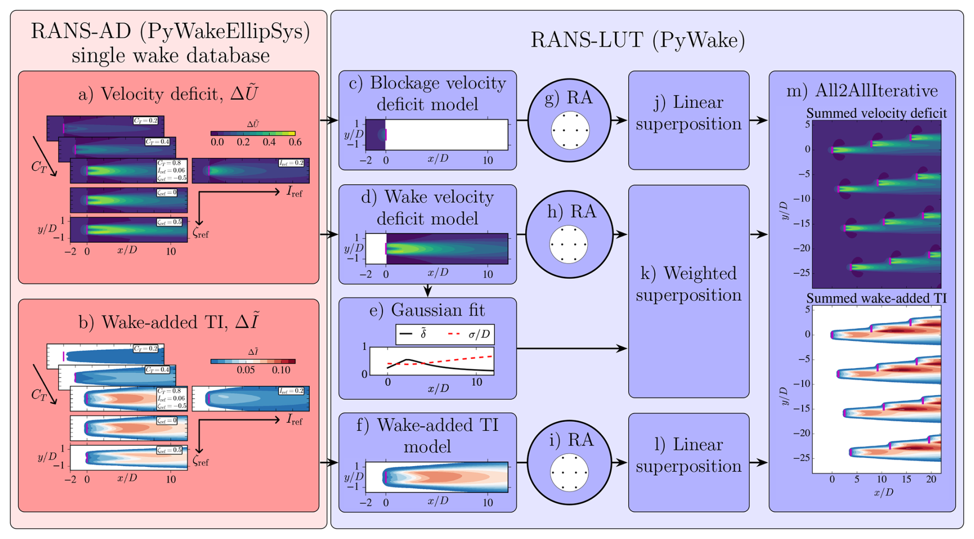
Figure 2 Overview of RANS-AD single-wake database (a, b) and workflow of the proposed RANS-LUT surrogate model (c–m). Contour plots depict the flow at hub height, and the magenta rectangle illustrates the location of the AD model. Panels (g)–(i) are rotor-averaging (RA) operators. An example of a final result of the iterative method All2AllIterative is shown in (m).

2.3.1 Single-turbine model

The single-turbine deficit and wake-added TI model by Criado Risco et al. (2023) is built by normalizing the streamwise velocity deficit and added TI fields with the background flow, such that for a single RANS simulation

$$\begin{array}{}\text{(7)}& \begin{array}{rl}{\displaystyle }& {\displaystyle }\mathrm{\Delta }\stackrel{\mathrm{̃}}{U}\left({\mathit{x}}^{\prime }\right)={\displaystyle \frac{U\left({\mathit{x}}^{\prime }\right)-U_b\left(z^{\prime }\right)}{U_b\left(z^{\prime }\right)}},\\ {\displaystyle }& {\displaystyle }\mathrm{\Delta }\stackrel{\mathrm{̃}}{I}\left({\mathit{x}}^{\prime }\right)={\displaystyle \frac{\sqrt{\mathrm{2}/\mathrm{3}k\left({\mathit{x}}^{\prime }\right)}-\sqrt{\mathrm{2}/\mathrm{3}{k}_b\left(z^{\prime }\right)}}{U_b\left(z^{\prime }\right)}},\end{array}\end{array}$$

with normalized deficit $\mathrm{\Delta }\stackrel{\mathrm{̃}}{U}$ and added TI $\mathrm{\Delta }\stackrel{\mathrm{̃}}{I}$, computed from streamwise velocity U and turbulent kinetic energy k. The background flow is denoted by ⋅_b and corresponds to a simulation with C_T=0. All variables are given in the turbine hub coordinate system ${\mathit{x}}^{\prime }=(\mathit{x}-{\mathit{x}}_{\mathrm{H}})/D$, with turbine hub position x_H in the RANS frame of reference and $\mathit{x}=(x,y,z)$.

As illustrated in Fig. 2a and b, the RANS-LUT wake model employed here is built from a RANS-AD single-wake database 𝒟_L, which is a discrete collection of numerical solutions sampled across a range of thrust coefficients, inflow turbulence intensities, and stability parameters. To reconstruct the continuous velocity deficit and turbulence intensity fields from these discrete samples, a multi-dimensional interpolation operator ℐ is employed. The final single-wake model takes the functional form

$$\begin{array}{}\text{(8)}& \mathrm{\Delta }\stackrel{\mathrm{̃}}{U},\mathrm{\Delta }\stackrel{\mathrm{̃}}{I}=\mathcal{I}({\mathit{x}}^{\prime },C_{\mathrm{T}},I_{\text{ref}},{\mathit{\zeta }}_{\text{ref}}|{\mathcal{D}}_{\mathrm{L}}),\end{array}$$

where ℐ maps the discrete entries in 𝒟_L to a continuous domain. Within PyWake this is done using the xarray package (Hoyer and Hamman, 2017) for multi-dimensional data handling. However, PyWake's native 1D grid interpolator is employed by collapsing all dimensions into a 1D array, which is faster than the multi-dimensional xarray interpolator. Furthermore, we use linear interpolation, due to its robustness and speed. To optimize memory usage, 𝒟_L retains only the vertical CFD layers spanning the rotor-swept area – defined by the range between the minimum and maximum tip heights across all turbines within a farm. For wind farms with heterogeneous turbine types, 𝒟_L is expanded to include specific entries for each turbine model. Figure 2c and d show how the single-wake deficit database is split into up- and downstream regions to build PyWake blockage and wake deficit models. This results in some effects related to blockage, as for example the speed-up in wind speed around the turbine wake, becoming part of the wake deficit model. As depicted in Fig. 2f, this split is not done for the wake-added TI model.

2.3.2 Wind farm flow field

To move from the non-dimensional quantities provided by the single-wake model in Eq. (8) to a physical representation of the flow field, they must be scaled by some reference inflow values, which are referred to as effective wind speed, $\widehat{U}$, and TI, $\widehat{I}$, in PyWake. As turbines inside a farm respond to the local waked inflow, we compute quantities at each rotor location. In general the effective wind speed at the ith turbine in PyWake in the wind farm coordinate system is given by

$$\begin{array}{}\text{(9)}& \textcolor{red}{}\end{array}$$

$$\begin{array}{}\text{(10)}& \begin{array}{rl}& \langle {\widehat{U}}_j\mathrm{\Delta }{\stackrel{\mathrm{̃}}{U}}_j{\rangle }_{A_i}=\\ & \sum _n{w}_n{\widehat{U}}_j\mathrm{\Delta }\stackrel{\mathrm{̃}}{U}({\mathit{x}}_{i,n}-{\mathit{x}}_{\mathrm{H},j},C_{\mathrm{T}}({\widehat{U}}_j),{\widehat{I}}_j,{\mathit{\zeta }}_{\text{ref}}),\end{array}\end{array}$$

where wake deficits $\mathrm{\Delta }{\stackrel{\mathrm{̃}}{U}}_{\mathrm{W}}$ from upstream turbines 𝒲 and blockage deficits $\mathrm{\Delta }{\stackrel{\mathrm{̃}}{U}}_{\mathrm{B}}$ from downstream turbines ℬ are superimposed (self-induction is excluded) and rotor-averaged $\langle \cdot {\rangle }_{A_i}$ separately and deducted from the wind farm background flow, which is evaluated at the rotor center U_b(x_H,i). This signifies that background flow variations over the rotor area (shear, veer) do not impact the effective wind speed and consequently neither turbine power nor thrust. Note that this differs from the way the RANS-AD reacts to the flow, which responds to the local variation over the AD instead, i.e $U_b\left({\mathit{x}}_i\right)-{\widehat{U}}_j\mathrm{\Delta }{\stackrel{\mathrm{̃}}{U}}_j({\mathit{x}}_{i,n}-{\mathit{x}}_{\mathrm{H},j})$. Rotor averaging, executed preceding superposition, is performed by weighing the scaled deficits $\widehat{U}\mathrm{\Delta }\stackrel{\mathrm{̃}}{U}$ over the rotor area A_i with weights w_n assigned to discrete sampling points, representing a numerical integration across the rotor disk where $\sum w_n=\mathrm{1}$. Here, the normalized deficits are scaled by the turbine local wind speed; however, in PyWake it is generally possible to switch to freestream scaling, meaning that ${\widehat{U}}_j=U_b\left({\mathit{x}}_{\mathrm{H},j}\right)$ in the above. Furthermore, superposition and rotor-averaging methods are allowed to differ between blockage and wake deficits in PyWake, and, whilst not used here, it is possible to introduce multi-dimensional thrust curves. Generally the background flow in PyWake is allowed to vary freely in space, yet here we ensure it follows the RANS inflow conditions that only include vertical shear following MOST:

$$\begin{array}{}\text{(11)}& {\displaystyle }{U}_b\left(z\right)=U_{\text{ref}}{\displaystyle \frac{\ln (z/z_{\mathrm{0}})-{\mathrm{\Psi }}_{\mathrm{m}}\left(\mathit{\zeta }\right)}{\ln (z_{\text{ref}}/z_{\mathrm{0}})-{\mathrm{\Psi }}_{\mathrm{m}}\left({\mathit{\zeta }}_{\text{ref}}\right)}},\end{array}$$

with Ψ_m as the integrated normalized shear from MOST, as defined in van der Laan et al. (2017). The effective TI is only computed using upstream turbines:

$$\begin{array}{}\text{(12)}& \textcolor{red}{}\end{array}$$

where ⊕ denotes the superposition of background with added TI. As the single-wake database underlying the RANS-LUT model is generated through a parametric variation in inflow TI, our approach inherently assumes that turbines respond identically to ambient inflow and wake-added TI.

Due to the inclusion of up- and downstream effects, an iterative approach needs to be employed to obtain the effective wind speed and TI at all turbines. As shown in Fig. 2m, here we use PyWake's All2AllIterative solver. Once the operating conditions of each turbine have been determined, they are fixed, and the final wind farm flow field at a point x_i is determined by aggregating contributions from all turbines 𝒩–omitting all other dimensions except x for $\mathrm{\Delta }\stackrel{\mathrm{̃}}{U},\mathrm{\Delta }\stackrel{\mathrm{̃}}{I}$:

$$\begin{array}{}\text{(13)}& \textcolor{red}{}\text{(14)}& \textcolor{red}{}\end{array}$$

2.3.3 Superposition methods

As deficits and power production scale with the effective wind speed, the accuracy of our RANS-LUT model predictions strongly depends on our choice of superposition models. Whilst Eq. (9) shows an explicit dependency on the deficit superposition models, their is also an implicit connection to the TI superposition, as the normalized deficit ΔU is a function of the effective TI $\widehat{I}$. While Criado Risco et al. (2023) found that linear superposition of velocity deficits and wake-added TI yielded the most accurate results, Delvaux et al. (2024) identified the superposition of the maximum added TI – ${\widehat{I}}_i=I_b\left({\mathit{x}}_{\mathrm{H},i}\right)+{max}_j\langle \mathrm{\Delta }{\stackrel{\mathrm{̃}}{I}}_j\rangle$ – as optimal; however they also utilized a different definition of wake-added TI, namely $\mathrm{\Delta }\stackrel{\mathrm{̃}}{I}=\sqrt{\mathrm{2}/\mathrm{3}(k-k_b)}/U_b$. As we follow the one by Criado Risco et al. (2023) in Eq. (7), we similarly linearly superimpose wake-added TI contributions as depicted in Fig. 2l such that

$$\begin{array}{}\text{(15)}& {\widehat{I}}_i=I_b\left({\mathit{x}}_{\mathrm{H},i}\right)+\sum _{j\in \mathcal{W}}\langle \mathrm{\Delta }{\stackrel{\mathrm{̃}}{I}}_j{\rangle }_{A_i}.\end{array}$$

Since blockage deficits are limited, they are also linearly superimposed – a valid approach as demonstrated by Meyer Forsting et al. (2023).

As mentioned above, Criado Risco et al. (2023) similarly superimposed wake deficits linearly and found them to agree with RANS-AD simulations in terms of the wind farm velocity and TI fields. However, as shown in detail in Appendix B, we find that this is due to velocity superposition errors canceling those from using rotor center – $\langle \mathrm{\Delta }{\stackrel{\mathrm{̃}}{U}}_j\rangle =\mathrm{\Delta }\stackrel{\mathrm{̃}}{U}\left({\mathit{x}}_{\mathrm{H},j}\right)$ – instead of rotor-averaged values. As reported by Zong and Porté-Agel (2020), linear superposition overestimates wake deficits in deep arrays, and they consequently devised a momentum-deficit-conserving superposition method instead, which effectively acts as a weighted sum, such that the combined wind farm deficit is given by

$$\begin{array}{}\text{(16)}& \mathrm{\Delta }U=\sum _i{\displaystyle \frac{u_c^i}{U_c}}\mathrm{\Delta }{u}^i,\end{array}$$

where lower- and uppercase letters refer to the single-turbine and combined wind farm velocities, respectively. The weights are given by the ratio between single-turbine u_c and wind farm U_c wake convection velocities, which are determined by performing an integral over the plane perpendicular to the mean flow, A_⟂:

$$\begin{array}{}\text{(17)}& U_c={\displaystyle \frac{{\int }_{A_{⟂}}(U_b-\mathrm{\Delta }U)\mathrm{\Delta }U}{{\int }_{A_{⟂}}\mathrm{\Delta }U}}.\end{array}$$

For a single turbine just replace with lowercase letters. Equations (16) and (17) are coupled, thus requiring an iterative approach. Hence, to employ the weighted sum, cross-plane integrals need to be performed for single-turbine wakes and the combined wind farm flow at every iteration until convergence. If the cross-plane integrals are performed numerically, the computational cost would be prohibitive. PyWake circumvents this by employing analytical solutions based on assuming Gaussian-shaped wake deficits, defined here as

$$\begin{array}{}\text{(18)}& \mathrm{\Delta }u=\mathit{\delta }\exp \left(-{\displaystyle \frac{r^{\mathrm{2}}}{\mathrm{2}{\mathit{\sigma }}^{\mathrm{2}}}}\right),\end{array}$$

with centerline deficit δ, cross-wind distance r, and wake expansion σ. Zong and Porté-Agel (2020) already showed that for a single Gaussian wake there is an analytical solution to Eq. (17), as it has a finite integral. Here, we show that there is also an analytical solution to the wind farm flow; substituting Eq. (16) into Eq. (17) and assuming that U_b does not vary over A_⟂, the update of $U_c^{(n+\mathrm{1})}$ can be written entirely in terms of single-wake parameters that can be precomputed:

$$\begin{array}{}\text{(19)}& \begin{array}{rl}{\displaystyle }& {\displaystyle }{U}_c^{(n+\mathrm{1})}=U_b-{\displaystyle \frac{\mathrm{1}}{U_c^{\left(n\right)}}}{\displaystyle \frac{{\int }_{A_{⟂}}{\left({\sum }_i{u}_c^i\mathrm{\Delta }{u}_i\right)}^{\mathrm{2}}}{{\int }_{A_{⟂}}{\sum }_i{u}_c^i\mathrm{\Delta }{u}_i}}=U_b-{\displaystyle \frac{\mathrm{1}}{U_c^{\left(n\right)}}}\\ {\displaystyle }& {\displaystyle }\times {\displaystyle \frac{{\sum }_i{\left(u_c^i{\mathit{\delta }}_i\sqrt{\mathit{\pi }}{\mathit{\sigma }}_i\right)}^{\mathrm{2}}+\mathrm{2}{\sum }_i{\sum }_{j<i}\left(u_c^i{u}_c^j{\mathit{\delta }}_i{\mathit{\delta }}_j{\mathcal{I}}_{ij}\right)}{{\sum }_i{u}_c^i{\mathit{\delta }}_i\mathrm{2}\mathit{\pi }{\mathit{\sigma }}_i^{\mathrm{2}}}}\\ {\displaystyle }& {\displaystyle }{\mathcal{I}}_{ij}={\displaystyle \frac{\mathrm{2}\mathit{\pi }{\mathit{\sigma }}_i^{\mathrm{2}}{\mathit{\sigma }}_j^{\mathrm{2}}}{{\mathit{\sigma }}_i^{\mathrm{2}}+{\mathit{\sigma }}_j^{\mathrm{2}}}}\exp \left(-{\displaystyle \frac{d_{ij}^{\mathrm{2}}}{\mathrm{2}({\mathit{\sigma }}_i^{\mathrm{2}}+{\mathit{\sigma }}_j^{\mathrm{2}})}}\right)\\ {\displaystyle }& {\displaystyle }{d}_{ij}=\sqrt{(y_{\mathrm{H},i}-y_{\mathrm{H},j}{)}^{\mathrm{2}}+(z_{\mathrm{H},i}-z_{\mathrm{H},j}{)}^{\mathrm{2}}},\end{array}\end{array}$$

where ℐ_ij represents the interaction between two wakes, meaning that if the combined deficit downstream of the ith turbine is to be computed, the interaction of its single wake with all preceding wakes (i<j) needs to be determined. As this nested sum can become expensive, small deficits less than 1 % of U_b are skipped and added linearly ($u_c^i=U_c^{\left(n\right)}$). As the superposition model assumes that the pressure has fully recovered ($\partial p/\partial x\approx \mathrm{0}$), it does not hold in the near-wake, causing the algorithm to become unstable, as locally the individual wake convection velocity might exceed that of the combined wakes. Referring to Eq. (19), if $u_c>U_c^{\left(n\right)}$, U_c→0, as the numerator grows faster than the denominator, and U_c continues to drop. Since $u_c>U_c^{\left(n\right)}$ implies that individual wakes are convected faster than the background flow and that momentum deficit would be created during superposition (see Eq. 16), we enforce $u_c\le U_c^{\left(n\right)}$. This means that the weights – $u_c/U_c^{\left(n\right)}$ – in the superposition method do not exceed 1. The iterations are initialized by setting $U_c={max}_i\left(u_c^i\right)$, and stopped when $max\left|\right(U_c^{(n+\mathrm{1})}-U_c^{\left(n\right)})/U_c^{\left(n\right)}|<{\mathrm{10}}^{-\mathrm{3}}$, or five iterations have been completed.

Due to its accuracy, speed, and numerical stability, we adopt the analytical approach in our RANS-LUT model by fitting Gaussian profiles to the RANS-AD database. The fitting is performed over the downstream plane at hub height, $z^{\prime }=\mathrm{0}$ and $\mathrm{2}\le x^{\prime }\le \mathrm{100}$, with an additional fit at $x^{\prime }=\mathrm{0}$ where the magnitude is limited to the axial induction from 1D momentum theory; see Fig. 2e. Subsequently, the normalized wake expansion, $\mathit{\sigma }/D$, and centerline deficit, $\stackrel{\mathrm{̃}}{\mathit{\delta }}$, are provided by additional LUT-based surrogate models:

$$\begin{array}{}\text{(20)}& {\displaystyle }\mathit{\sigma }/D,\stackrel{\mathrm{̃}}{\mathit{\delta }}=\mathcal{L}\left(x^{\prime },C_{\mathrm{T}},I_{\text{ref}},{\mathit{\zeta }}_{\text{ref}}|{\mathcal{G}}_{\mathrm{L}}\right),\end{array}$$

where δ from the RANS-AD simulations is normalized by the hub height wind speed. It should be noted that the assumption of the Gaussian velocity deficit is only applied to determine the superposition weights that are employed to superpose the velocity deficit shapes of the RANS-LUT model. The performance of the weighted superposition method and effect of enforcing the $u_c\le U_c^{\left(n\right)}$ limit is further discussed in Sect. B.

Finally, in this work we use a rotor-averaging model based on a Gaussian quadrature method with eight points, which is sufficient to obtain a rotor-average wind speed with an error of 0.65 % (Pedersen et al., 2023).

3 Results and discussion

The RANS-AD and RANS-LUT surrogate models have been employed to simulate a wind turbine row and a square wind farm for different turbine spacing and inflow cases, as defined in Sect. 2.1. The RANS-AD results are used to evaluate the RANS-LUT model performance in terms of the flow (Sect. 3.1 and 3.2), turbine power performance (Sect. 3.3), and wind farm efficiency (Sect. 3.4). RANS-LUT model errors in streamwise velocity, ϵ_U, TI, ϵ_I, turbine power, ϵ_P,i, and wind farm efficiency, ϵ_η, are computed as the difference between the models normalized by the freestream values:

$$\begin{array}{}\text{(21)}& {\mathit{ϵ}}_{\mathrm{U}}={\displaystyle \frac{U_{\text{LUT}}-U_{\text{RANS}}}{U_{\text{ref}}}},\end{array}$$

$$\begin{array}{rl}{\displaystyle }{\mathit{ϵ}}_{\mathrm{I}}& {\displaystyle }={\displaystyle \frac{\sqrt{\frac{\mathrm{2}}{\mathrm{3}}{k}_{\text{LUT}}}-\sqrt{\frac{\mathrm{2}}{\mathrm{3}}{k}_{\text{RANS}}}}{U_{\text{ref}}}}=I_{\text{LUT}}-I_{\text{RANS}},\\ {\displaystyle }{\mathit{ϵ}}_{\mathrm{P},i}& {\displaystyle }={\displaystyle \frac{P_{i,\text{LUT}}-P_{i,\text{RANS}}}{P_{\text{ref}}}},\\ {\displaystyle }{\mathit{ϵ}}_{\mathit{\eta }}& {\displaystyle }={\displaystyle \frac{{\sum }_{i=\mathrm{1}}^{i=N}{P}_{i,\text{LUT}}-{\sum }_{i=\mathrm{1}}^{i=N}{P}_{i,\text{RANS}}}{N{P}_{\text{ref}}}}={\mathit{\eta }}_{\text{LUT}}-{\mathit{\eta }}_{\text{RANS}},\end{array}$$

with i as the turbine index, N as the total number of turbines, P_i as the turbine power of turbine i, P_ref as the turbine power obtained from the power curve as defined by the simple turbine model from Eq. (1), and η as the wind farm efficiency.

3.1 Flow

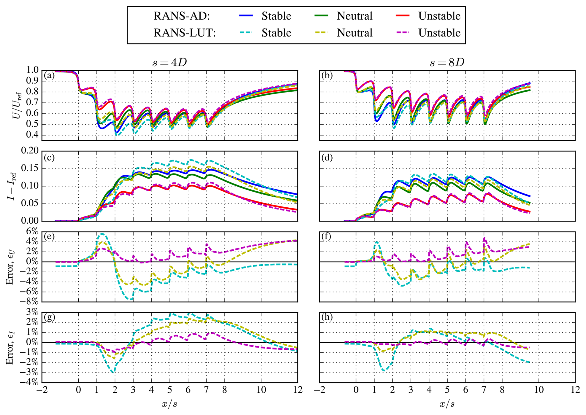
Figure 3 depicts the rotor-averaged streamwise velocity and wake-added TI obtained from the results of the turbine row consisting of eight turbines. Results are shown for the three stability cases and two turbine spacings, s=4D and s=8D. A below-rated wind speed of 11 m s⁻¹ is used, which means that all turbines operate at the same thrust coefficient of C_T=0.8. Hence, the wake shapes applied in the RANS-LUT model only change by wake-added TI, but the magnitude in wake deficit still varies due to the wake superposition and effective wind speed scaling. Figure 3e–h depict the RANS-LUT model errors in streamwise velocity and wake-added TI. Overall, the RANS-LUT model captures the trend of both the streamwise velocity and wake-added TI in terms of downstream development and effect of atmospheric stability. The RANS-LUT model mainly overpredicts the wake-added TI inside the turbine row but underpredicts the wake-added TI in the wind farm wake for the turbine row with the smallest spacing, as shown in Fig. 3e. The opposite trend is obtained for the streamwise velocity errors for the smallest spacing and the stable and neutral cases (Fig. 3e and f). The largest absolute errors are 5 % and 2.5 % for the streamwise velocity (Fig. 3e and f) and wake-added TI (Fig. 3g and h), respectively. It is also worth noting that the errors in the wind farm wake can be larger than the errors inside the turbine row, as obtained for the unstable case with 4D spacing (Fig. 3e and g). The RANS-LUT model includes blockage effects and predict similar values of upstream rotor-averaged streamwise velocity for the neutral and unstable cases, as shown in Fig. 3e and f, for $x/s<\mathrm{0}$. However, the RANS-LUT model overpredicts the wind farm blockage for the stable case by about 1 %, which is not fully understood.

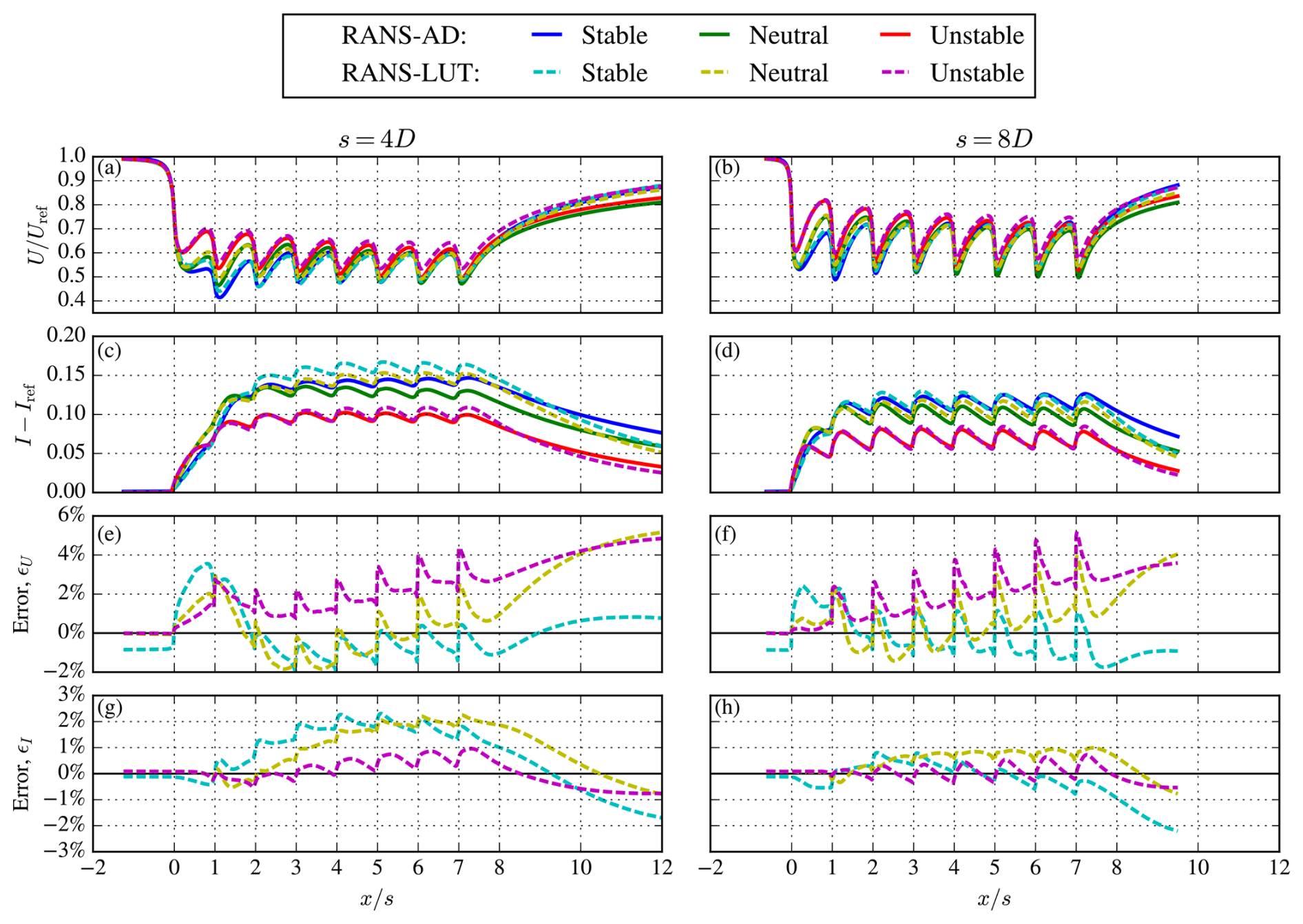
Figure 3 Rotor-averaged streamwise velocity (a, b), wake-added TI (c–d), and corresponding model errors (e–h) in a turbine row with 4D and 8D turbine spacing and $U_{\text{ref}}=\mathrm{11}\mathrm{m}{\mathrm{s}}^{-\mathrm{1}}$ (constant C_T=0.8).

Figure 4 is the same as Fig. 3, but an above-rated wind speed is applied, resulting in a varying turbine thrust coefficient. Similar observations can be made as discussed for Fig. 3, but the errors in streamwise velocity and wake-added TI are higher for the above-rated case, where the largest absolute errors are about 8 % and 3 %, respectively, obtained for the stable case.

Figure 4 Same as Fig. 3 for $U_{\text{ref}}=\mathrm{14}\mathrm{m}{\mathrm{s}}^{-\mathrm{1}}$ (variable C_T).

One can remove the error of looking up the wrong velocity deficit shape in the RANS-LUT model by simulating the below-rated wind speed case (constant C_T) with prescribed wake-added TI values obtained from the RANS-AD model. The resulting normalized stream-wise velocity and corresponding error are depicted in Fig. 5. The largest absolute errors in the RANS-LUT model are obtained for the unstable case with 8D spacing and are about 1 % higher in magnitude as calculated for the case where the wake-added TI is not prescribed by the RANS-AD model, as shown in Fig. 3. This indicates that an overestimation in wake-added TI can slightly reduce the error in stream-wise velocity deficit. However, the main source of error is the velocity deficit superposition method, as shown in Fig. B1, and not the error made by looking up the wrong wake shape due to an overprediction of wake-added TI.

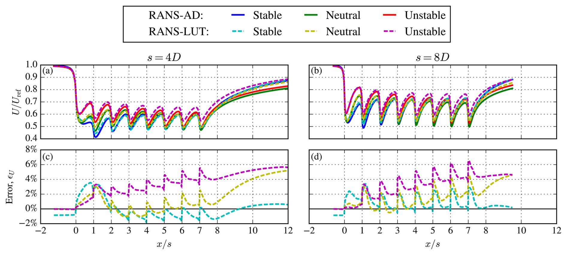
Figure 5 Rotor-averaged streamwise velocity (a, b) for prescribed wake-added TI values from RANS-AD and corresponding model errors (c, d) in a turbine row with 4D and 8D turbine spacing and $U_{\text{ref}}=\mathrm{11}\mathrm{m}{\mathrm{s}}^{-\mathrm{1}}$ (constant C_T=0.8).

Figure 6 depicts the streamwise velocity and wake-added TI at hub height for the wind farm with 8D turbine spacing and a below-rated wind speed. Results of the RANS-LUT and RANS-AD models are shown for all three stability cases. A wind direction of 279° is selected where the downstream turbines operate in a partial wake depending on the stability conditions. The streamwise velocity of the RANS-AD model (Fig. 6a–c) shows that the wakes are more narrow for stable cases compared to the neutral and unstable cases. As a result, the wake effects of the stable case are less pronounced compared to the other stability cases, which is shown in more detail in Sect. 3.4 in terms of wind farm efficiency. The RANS-LUT model is able to capture this trend, although it overpredicts the wake-added TI compared to the RANS-AD model for the stable and neutral cases, as shown in Fig. 6g, j, h, and k. In addition, the RANS-LUT model flow fields are less smooth compared to the RANS-AD model flow fields, mainly visible for the stable and neutral cases, which is a consequence of not solving the RANS and turbulence transport equations.

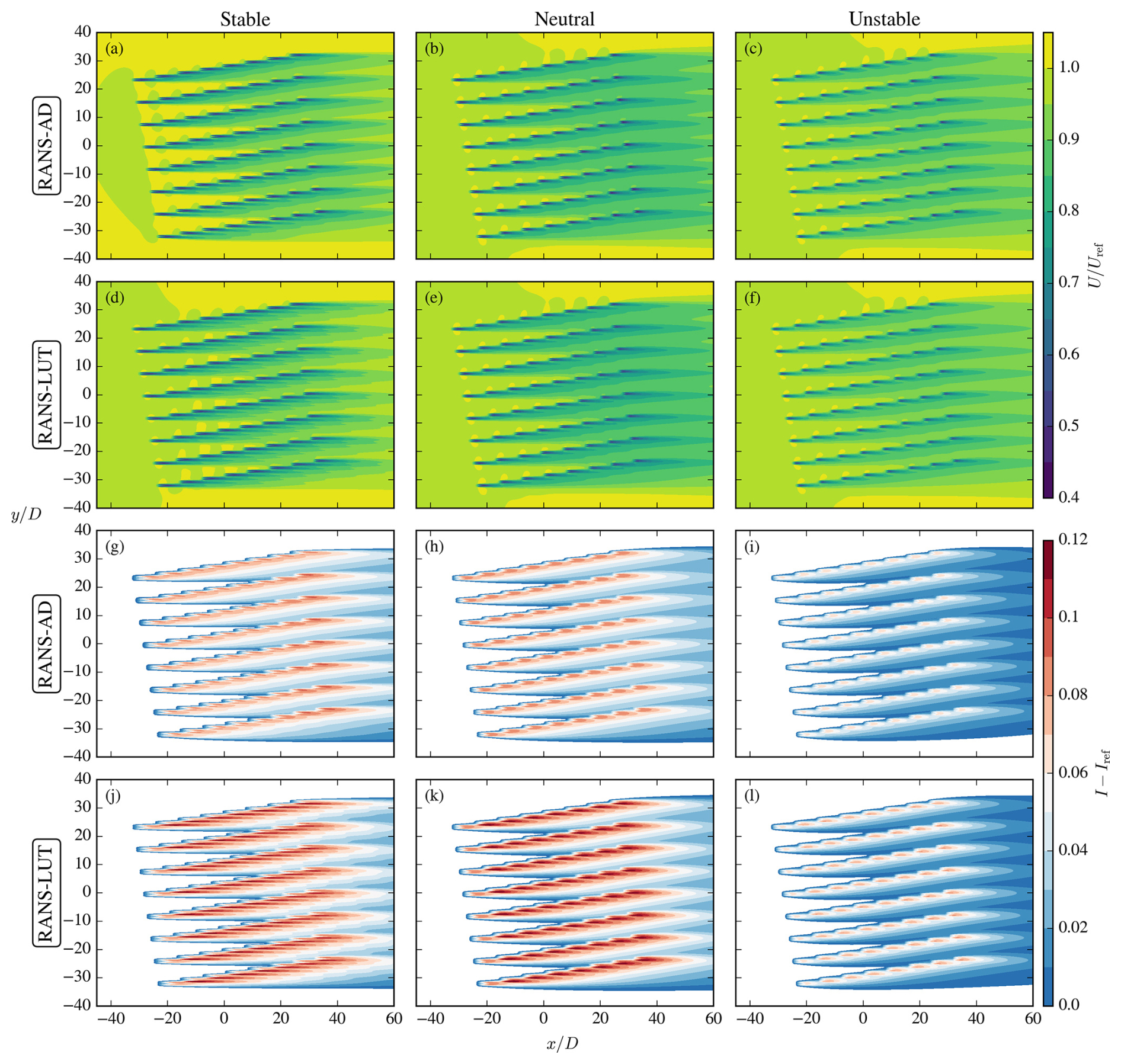
Figure 6 Flow at hub height in terms of streamwise velocity (a–f) and wake-added TI (g–l) for RANS-AD and RANS-LUT models, a wind farm with 8D turbine spacing, and $U_{\text{ref}}=\mathrm{11}\mathrm{m}{\mathrm{s}}^{-\mathrm{1}}$ (constant C_T=0.8).

3.2 Consequence of not including wake-added turbulence

In order to quantify the impact of wake-added turbulence, the RANS-LUT model has been employed without wake-added TI for the wind turbine rows with different turbine spacing, atmospheric stability cases, and a below-rated wind speed (constant C_T). This means that the employed velocity deficit wake shape is the same for all turbines per stability case. Results of rotor-averaged streamwise velocity and the corresponding model error are depicted in Fig. 7. Figure 7a and b show that the absence of wake-added TI in the RANS-LUT model leads to larger velocity deficits compared to the RANS-AD model. The removal of wake-added TI results in large model errors in the rotor-averaged streamwise velocity that grows with downstream distance inside the wind farm up to −22 %, which is more than 3 times as large as largest error obtained from the RANS-LUT model including wake-added TI for the same case (Fig. 3f). Hence, it is important to include wake-added TI LUTs in the RANS-LUT model.

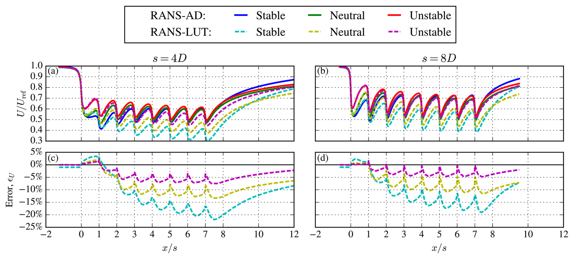
Figure 7 Rotor-averaged streamwise velocity (a, b) and corresponding model errors (c, d) in a turbine row with 4D and 8D turbine spacing and $U_{\text{ref}}=\mathrm{11}\mathrm{m}{\mathrm{s}}^{-\mathrm{1}}$ (constant C_T), without wake-added TI LUTs.

3.3 Wind turbine power

Figure 8 depicts the turbine power of the simulated wind turbine row for two wind turbine spacings, a below- and above-rated wind speed, and all three stability cases. The maximum absolute errors are 5.3 % and 20 % for the below- and above-rated wind speed cases, both obtained for the fourth turbine. In terms of mean absolute error in power of all turbines and cases, we obtain a values of 3.4 %.

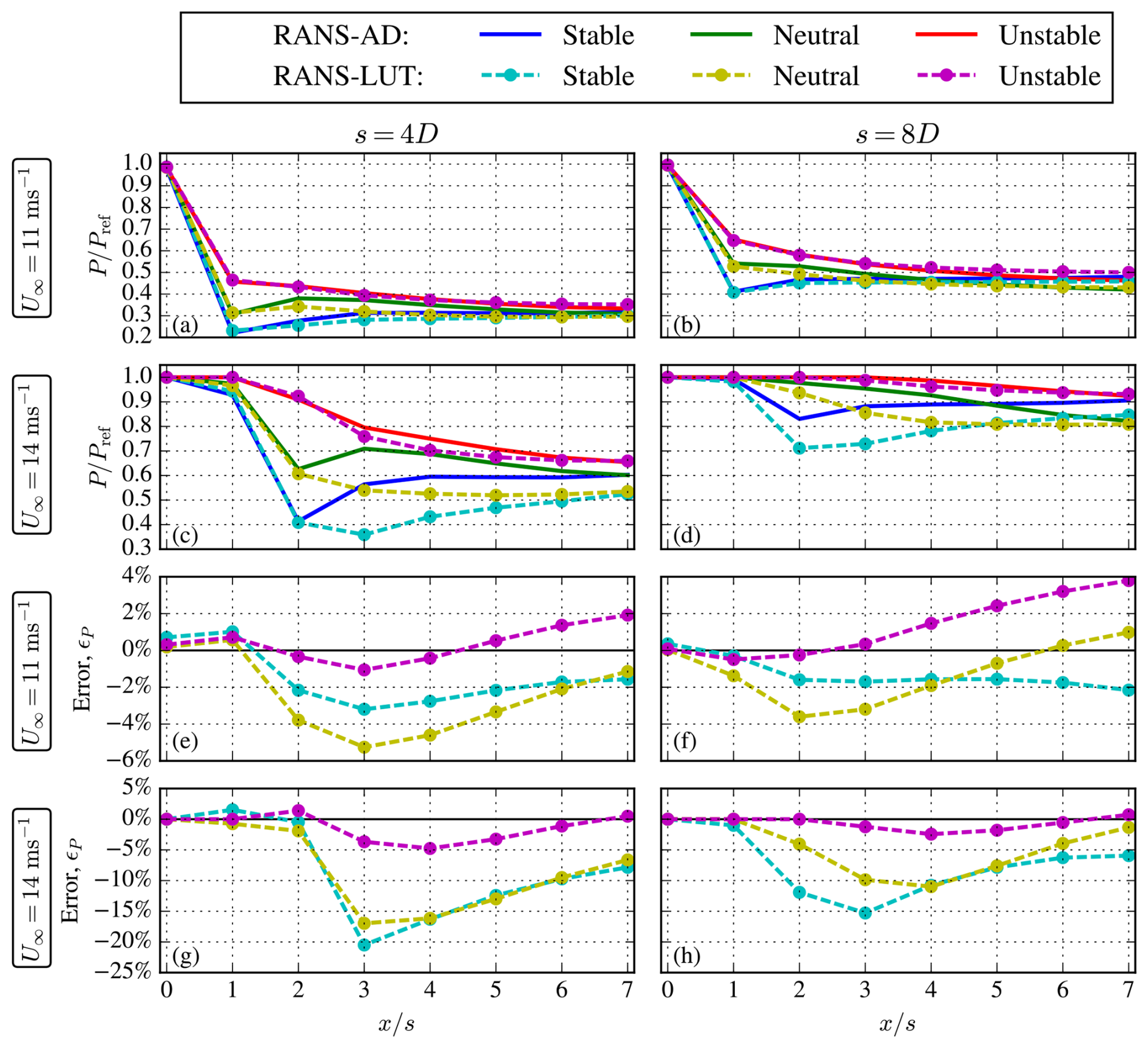
Figure 8 Wind turbine power (a–d) and RANS-LUT model error (e–h) of a turbine row with 4D and 8D turbine spacing and $U_{\text{ref}}=\mathrm{11}\mathrm{m}{\mathrm{s}}^{-\mathrm{1}}$ and $U_{\text{ref}}=\mathrm{14}\mathrm{m}{\mathrm{s}}^{-\mathrm{1}}$.

It should be noted that the RANS-LUT model errors in the rotor-averaged wind speed and turbine power can be opposite in sign, which is a counterintuitive result. For example, the error in rotor-averaged wind speed of the unstable case for an above-rated inflow wind speed is mostly positive (Fig. 4e and f), while the corresponding errors in power are negative for the fourth, fifth, and sixth turbine (Fig. 8g and h). The reason for the possibility of opposite sign errors in wind speed and power is related to a difference in power calculation method employed by the RANS-AD and RANS-LUT models. The RANS-LUT model follows the power calculation method in PyWake, which determines the power from the power curve using an effective wind speed at the turbine location that represents the effects of all neighboring turbines excluding its own induction, as explained in Sect. 2.3.2. The latter is not possible for a wind farm flow based on CFD since the inflow wind speed at the turbine location is undefined for a wind farm. Instead, an alternative power coefficient based on the actuator-disk-averaged wind speed is used from which the power can be obtained. The alternative power coefficient can be determined from 1D momentum theory (Calaf et al., 2010) or single RANS-AD simulations (van der Laan et al., 2015a); we employ the latter for the RANS-AD wind farm simulations in the present work.

3.4 Wind farm efficiency

The wind farm efficiency of the square wind farm as a function of wind direction is shown in Fig. 9 for the two turbine spacings, a below- and above-rated wind speed, and all three stability cases. Figure 9 shows that wind farm efficiency is lower for the below-rated wind speed and aligned wind direction as expected. However, the wind farm efficiency is not always the lowest for stable conditions because the wakes are narrower compared to neutral and unstable conditions and can therefore miss the downstream turbines more easily for wind directions in between row-aligned wind directions for the wind farm layout with 8D turbine spacing, as discussed previously in Sect. 3.1 using Fig. 6. This effect is also captured by the RANS-LUT model. The RANS-LUT model errors, as shown in Fig. 9c and d, are within ±3.0 % for the below-rated wind speed inflow. The highest errors are obtained for the row-aligned wind directions (270 and 315°); for the above-rated wind speed (14 m s⁻¹); and for the smallest turbine spacing, with a maximum error of 10 %.

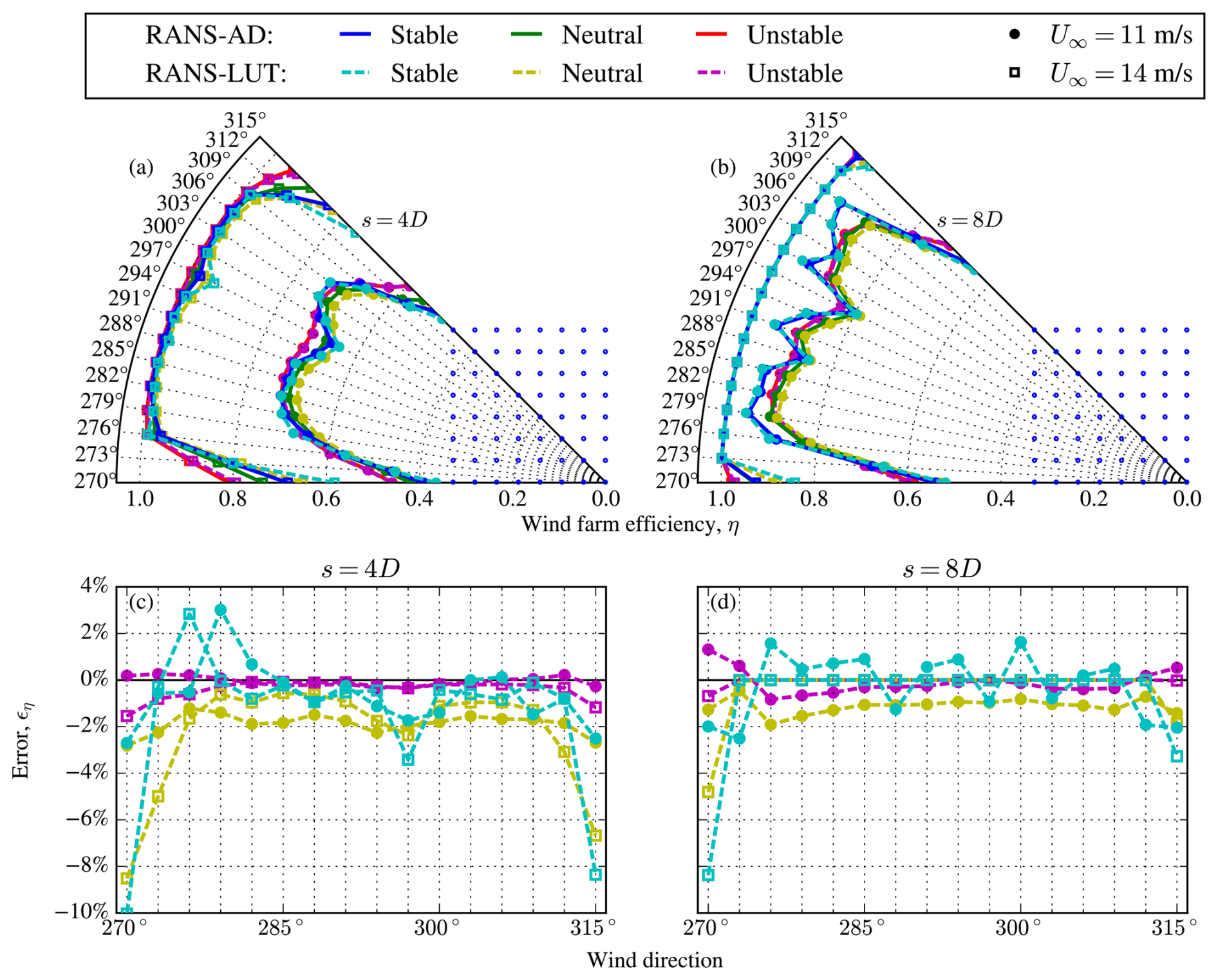
Figure 9 Wind farm efficiency (a, b) and corresponding RANS-LUT model error (c, d) for 8×8 wind farm with 4D (a, c) and 8D (b, d) turbine spacing and $U_{\text{ref}}=\mathrm{11}\mathrm{m}{\mathrm{s}}^{-\mathrm{1}}$ and $U_{\text{ref}}=\mathrm{14}\mathrm{m}{\mathrm{s}}^{-\mathrm{1}}$.

3.5 Computational effort and memory usage

The computational effort of the RANS-AD and RANS-LUT models is listed in Table 4 in terms of CPU hours and maximum memory usage. The simulations are run on the Sophia HPC cluster (Technical University of Denmark, 2019). It consists of nodes with 32 physical cores (2× 16-core AMD EPYC 7351) with either 128 or 256 GB RAM. The RANS-LUT model is run with a single core on a node with 256 GB RAM. The RANS-AD simulations are parallel and have been run with 532 and 696 cores for the wind farms with 4D and 8D spacing, respectively. The RANS-LUT surrogate model is 5 orders of magnitude faster than the RANS-AD model for the wind farm case with 8D spacing. The surrogate model also uses 2 orders of magnitude less memory. However, the RANS-LUT model is relatively slow and requires a large amount memory compared to an analytical engineering wake model. For example, running the TurbOPark analytical engineering wake model (Nygaard et al., 2020; Pedersen et al., 2022) in PyWake using the non-calibrated setup described in van der Laan et al. (2023) for the wind farm with 8D spacing requires 0.00074 CPU hours and 0.3 GB, which is about 25 times faster and 10 times less memory compared to the RANS-LUT model. Timings would be similar for any of the other analytical models available in PyWake. Here, the same iterative method for including both wake and blockage effects is applied as that used in the RANS-LUT model.

Table 4 Computational effort of RANS-LUT and RANS-AD models obtained from wind farms for stable conditions using 32 flow cases.

The CPU hours and memory usage of the RANS-LUT model increase with the number of turbines, N, as shown in Fig. 10. Results of additional simulations are shown for a square wind farm with 8D spacing for a single flow case (11 m s⁻¹ and 270°) using $N=\mathit{\{}{\mathrm{4}}^{\mathrm{2}},{\mathrm{8}}^{\mathrm{2}},{\mathrm{16}}^{\mathrm{2}},{\mathrm{32}}^{\mathrm{2}}\mathit{\}}$. Results of TurbOPark are also shown. Figure 10 shows that both the RANS-LUT and TurbOPark models require more CPU hours and memory with increasing number of turbines. For the largest wind farm using N=32², the RANS-LUT model requires 1 and 2 orders of magnitude more CPU hours and memory, respectively, compared to TurbOPark. For larger wind farms, the available 256 GB of node memory may be exceeded, and the RANS-LUT model cannot be run on the employed HPC. The CPU hours and memory usage also increase with N because the inclusion of blockage effects is calculated with an iterative method in PyWake (labeled as All2AllIterative), which scales roughly as 𝒪(N²) in terms of CPU hours and memory. One could investigate faster and less memory-intensive iterative methods, as for example the recently developed PropagateUpDownIterative method in PyWake, which uses iterative upwind and downwind steps where the memory scales as 𝒪(N). However, switching from All2AllIterative to PropagateUpDownIterative can lead to an increase in the mean absolute wind turbine power in the turbine rows of about 0.3 %. One could also reduce the number of points of the LUTs by simply removing data where they are not required, e.g., the near-wake region applicable to a wind farm layout with a relatively large turbine spacing. Other memory-reducing solutions could be in the form of an analytical model (Delvaux et al., 2024) or an artificial neural network (Schøler et al., 2023), both calibrated or trained with the single-wake database.

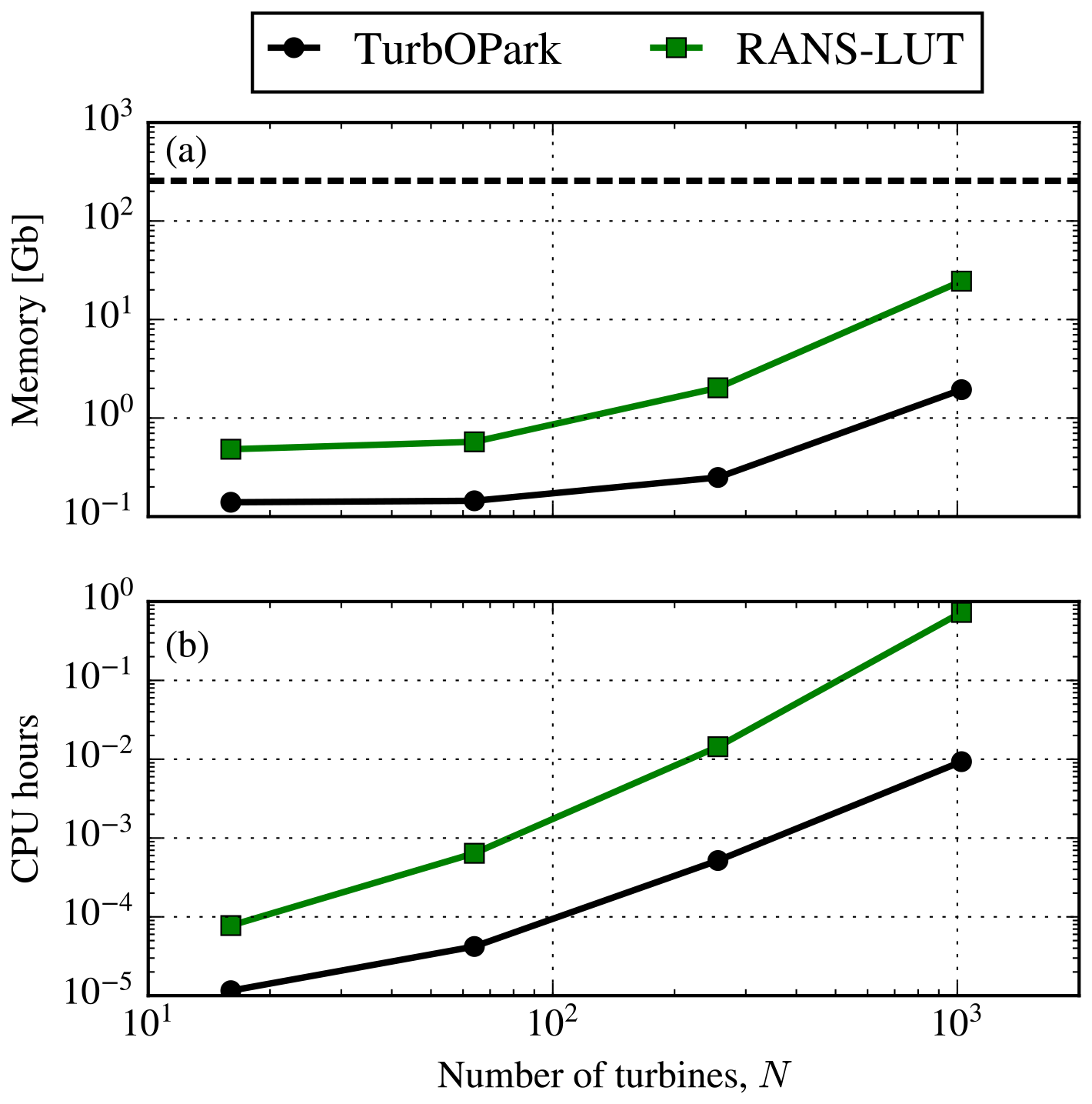
Figure 10 Computational effort of RANS-LUT and TurbOPark models with number of turbines using a single flow case ($U_{\text{ref}}=\mathrm{11}\mathrm{m}{\mathrm{s}}^{-\mathrm{1}}$ and 270°). Horizontal dashed line depicts memory limit of 256 GB.

3.6 Model limitations

The RANS-LUT surrogate model is based on RANS-AD single-wake simulations and will therefore inherit the limitations of the chosen RANS-AD method. In this work, we have applied a surface layer model following MOST. However, the applicability of MOST becomes less relevant for tall turbines that operate beyond the atmospheric surface layer, especially for stable conditions where the ABL is shallow. One could create a RANS-AD single-wake database based on an idealized ABL model including a prescribed pressure gradient, Coriolis, and an ABL height (van der Laan et al., 2024). However, it is not trivial to create a single-wake database for a large range of inflow TI required to represent wake-added TI in a wind farm simulation employing the RANS-LUT surrogate model. In other words, the RANS-LUT model assumption stating that the effects of inflow TI and wake-added TI are the same may not hold for an ABL inflow model. Furthermore, the deflection of the single wake due to the Coriolis-induced wind veer may require a superposition of lateral-velocity LUTs, which is currently not available in PyWake (v2.6.18).

RANS relies on a turbulence model that represents all turbulence scales. It is well known that RANS turbulence models can have model errors (Réthoré, 2009; van der Laan et al., 2015c; Baungaard et al., 2022b; Jigjid et al., 2025), and the development of better models is an active area of research. One could use a turbulence-resolving method as large-eddy simulation (LES) to create a single-wake database of mean velocity deficit and wake-added TI and develop a corresponding LES-LUT surrogate model. Such a model could also include a turbulence-length-scale dimension, which one could relate to atmospheric stability. Using LES to create a single-wake database is 3 to 4 orders of magnitude more expensive compared to RANS, but one may be able to obtain a more realistic wake model. The development of an LES-LUT surrogate model, as well as a validation of the RANS-LUT model, is recommended for future research.

4 Conclusions

A surrogate model of RANS-AD wind farm simulations is proposed, labeled as the RANS-LUT model, which is based on lookup tables of single-wake velocity deficit and wake-added TI flow fields including effects of atmospheric stability following MOST. The RANS-LUT model is evaluated against RANS-AD wind farm simulations for different inflow conditions and wind farms. The RANS-LUT model can capture the trend of RANS-AD wind farm simulations with respect to atmospheric stability, wind direction, and wind speed. The largest errors in rotor-averaged streamwise velocity and wake-added TI in a turbine row of eight turbines are 8 % and 3 %, respectively, and are obtained for an above-rated wind speed, stable conditions, and 4D turbine spacing. When wake-added TI is not used in the RANS-LUT model, then the largest error in streamwise velocity deficit increases to 22 %, which shows the necessity of including wake-added TI in the surrogate model. The errors in streamwise velocity lead to a mean absolute error in turbine power of 3.4 % for all turbine row cases. The wind farm case simulations consisting of 8×8 turbines reveal errors in wind farm efficiency up to 3 % below-rated, while above-rated a maximum absolute error of 10 % is obtained for a row-aligned wind direction and stable conditions. Good results for both velocity and power are achieved by using a momentum-based wake deficit superposition method in combination with a rotor-averaging model, which leads to a more consistent RANS surrogate model compared to using linear superposition without rotor averaging that relies on error cancellation. However, one of the main sources of error remains the wake deficit superposition. The applied velocity deficit superposition method is based on a simplified momentum equation, and one could investigate alternative superposition methods based on a more complex momentum equation, as for example proposed by (Bastankhah et al., 2021). The RANS-LUT model is about 10⁵ faster than the RANS-AD model, but it is still an order of magnitude slower than an engineering wake model using analytical wake shapes due to the need for interpolating and storing LUTs in the RANS-LUT model. More research is required to reduce the computational effort. In addition, the use of MOST is a limitation for large turbines that frequently operate beyond the atmospheric surface layer, especially for stable conditions. Future work could employ a more realistic inflow model including an ABL height and Coriolis, although it is not trivial how to generate a single-wake database for a large range of inflow TI for all conditions, which would be needed to represent wake-added TI when the RANS-LUT model is applied to a wind farm.

Appendix A: Nonlinear behavior of the thrust coefficient

In this section, the linearity of the thrust coefficient on the single-wake velocity deficit in RANS-AD simulations is investigated for neutral inflow conditions. To simplify the study, an AD model is employed based on a fixed normalized thrust force distribution (van der Laan et al., 2015c), obtained from a rotor-resolved CFD simulation of the DTU 10 MW reference turbine (Bak et al., 2013), and tangential forces are neglected. The effect of the thrust coefficient is investigated by scaling the normalized thrust force distribution accordingly.

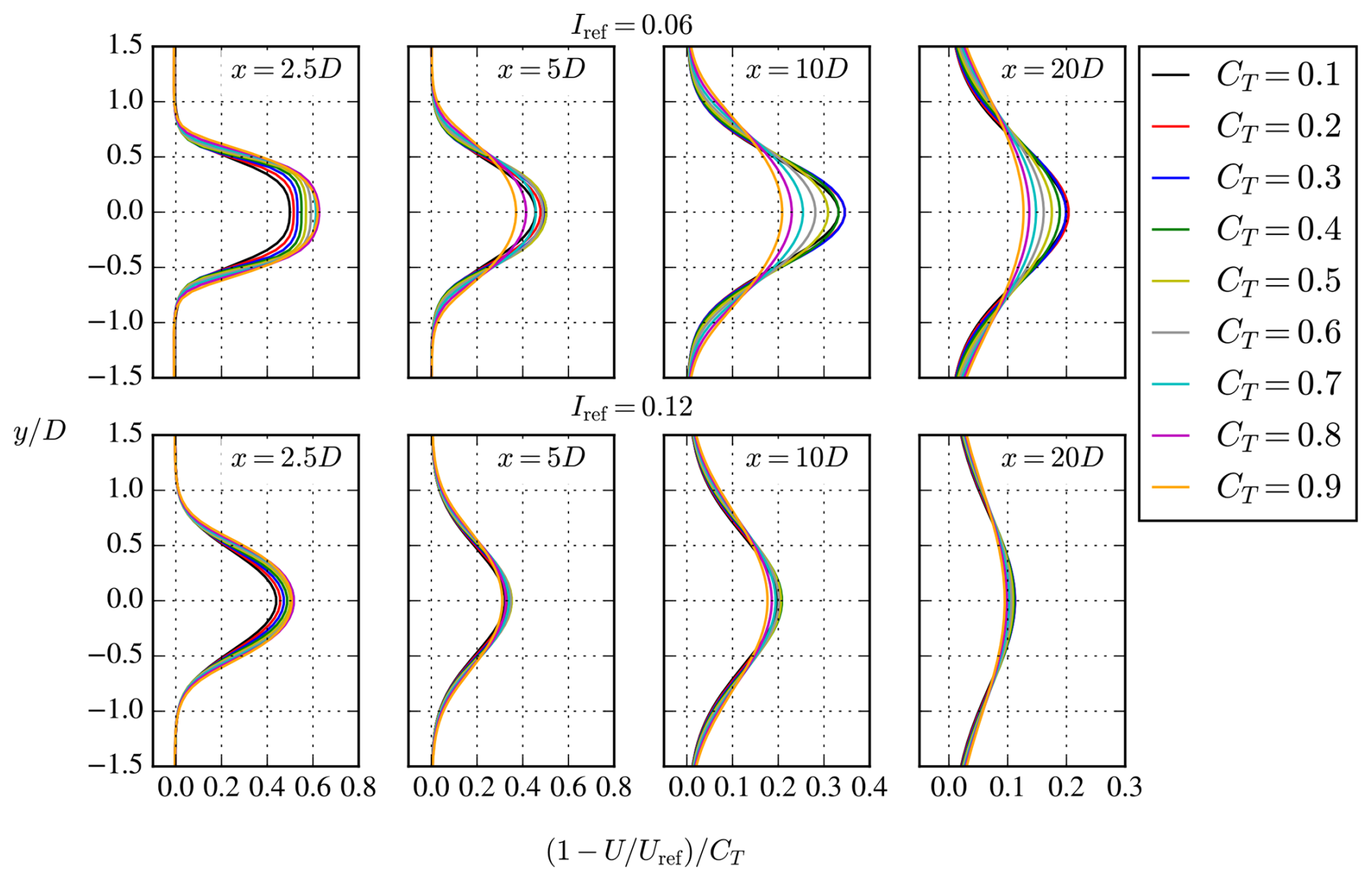
Figure A1 Effect of thrust coefficient on the single-wake velocity deficit, normalized by the thrust coefficient.

A conservative grid spacing of $D/\mathrm{16}$ is used. Figure A1 depicts the single-wake velocity deficit normalized by the thrust coefficient at four different downstream distances for two different ambient turbulence intensities and a range of thrust coefficients. It is clear that the velocity deficits do not collapse for constant ambient turbulence intensity, which shows the nonlinear behavior of the thrust coefficient. The wake recovery is enhanced with increasing thrust coefficient, and this leads to a nonlinear behavior of the thrust coefficient, which follows the same trend as the LES-derived near-wake length scale of Sørensen et al. (2015). Hence, the RANS-LUT surrogate model requires a thrust coefficient dimension in order to capture this effect.

Appendix B: Effect of wake superposition and rotor averaging

Figure B1 depicts results of the rotor-averaged streamwise velocity and turbine power of a wind turbine row consisting of eight turbines, with 4D and 8D spacing. The full RANS-AD model and the RANS-LUT surrogate model are employed with different combinations of velocity deficit superposition and rotor-averaging methods. The corresponding errors with respect to RANS-AD results are also plotted in Fig. B1. The most challenging inflow case is shown, corresponding to an above-rated wind speed (variable C_T) and stable conditions. Note that the rotor-averaging method of the RANS-LUT model refers to averaging the deficit at the turbine location to obtain the effective wind speed and wake-added TI, not the rotor-averaging method to obtain the flow as a post-step. Two different methods are applied: rotor center (RC), meaning no averaging, and rotor averaging (RA), using a Gaussian quadrature method that yields similar results to the AD polar grid of the RANS-AD model. The velocity deficit superposition methods are linear superposition (linear sum), weighted superposition of  Zong and Porté-Agel (2020) (weighted sum), and a weighted superposition where the weights do not exceed 1 (weighted sum limiter). The additional limiter ensures that the individual wakes are not convected faster than the background flow. Our implementation of the weighted superposition is discussed in detail in Sect. 2.3.3. Criado Risco et al. (2023) used a linear summation method without rotor averaging (RC), and their LUT flow predictions compared well to RANS-AD simulations, as also shown in Fig. B1a and b.

However, we find that this does not apply to power production, depicted in Fig. B1c and d, as it turns out that the favorable flow field predictions rely on superposition and effective wind speed errors canceling out. Linear summation leads to overestimating wind farm deficits in deep wakes (Zong and Porté-Agel, 2020); however at the rotor center the wind speed is lower compared to the rotor average, leading to lower deficits. This becomes clear when using linear superposition with the rotor-averaging model, which results in much larger errors compared to linear summation with the rotor center model, best visible in Fig. B1e, despite being more consistent with the RANS-AD simulation where rotor averaging is applied. When the weighted sum method is employed, the errors are reduced after the third or fourth turbine in the row. However, the weighted sum method can result in large errors in the near-wake because the superposition method weights are based on a simplified momentum equation, which is invalid in the near-wake, and we find that the weights can exceed 1. Therefore, we propose to limit the weights to not exceed 1 (i.e., the weights do not become larger than a linear superposition model). Figure B1e shows that the weighed sum method with the limiter does not produce the large errors in the near-wake and performs overall the best after the third turbine for both the flow and turbine power.

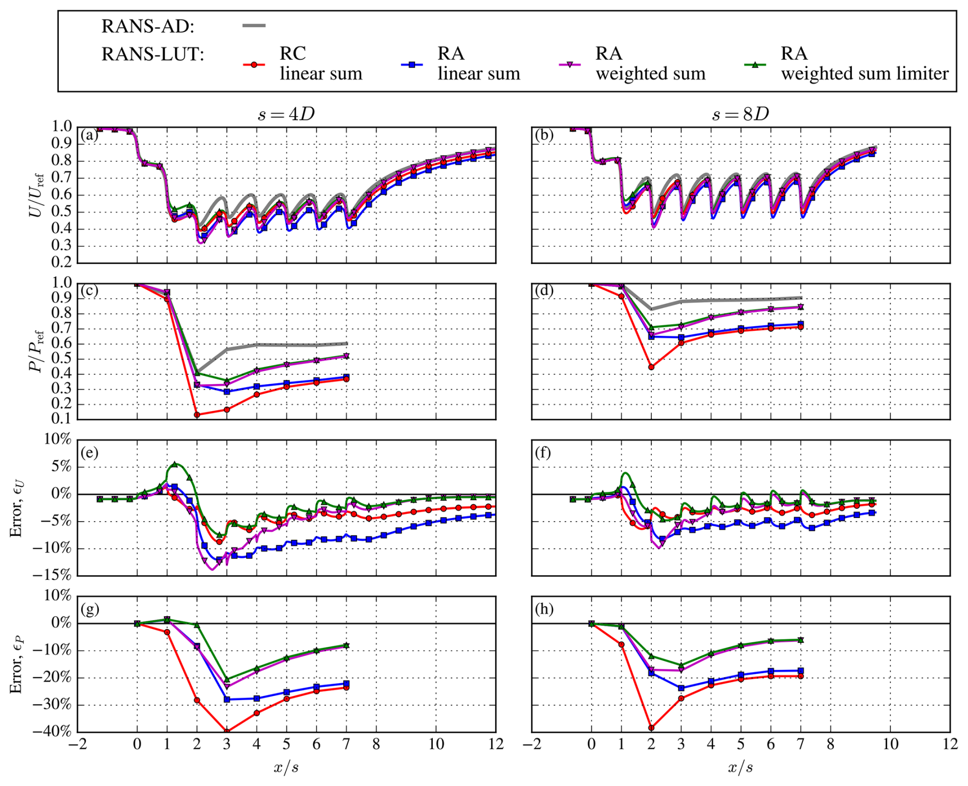
Figure B1 Rotor-averaged streamwise velocity (a, b) and wind turbine power (c, d) and corresponding model errors (e–h) in a turbine row with 4D and 8D turbine spacing, $U_{\text{ref}}=\mathrm{14}\mathrm{m}{\mathrm{s}}^{-\mathrm{1}}$ (variable C_T), and stable conditions. Results are shown for different rotor-averaging and superposition methods.

Appendix C: RANS-AD grid refinement study

The RANS-AD single-wake and wind farm simulations are performed with a grid that has a refined resolution around the AD of $D/\mathrm{8}$. A grid spacing of $D/\mathrm{8}$ to $D/\mathrm{10}$ is commonly used for neutral and unstable RANS-AD simulations employing EllipSys3D (van der Laan et al., 2015c, b; Baungaard et al., 2022a). However, for stable conditions, the grid resolution may need to be refined depending on the quantity of interest. Results of a grid refinement study of single RANS-AD simulations are shown in Fig. C1 using three grid resolutions – $D/\mathrm{4}$, $D/\mathrm{8}$, and $D/\mathrm{16}$ – and three stability inflow cases, as defined in Sect. 2.1. A below-rated inflow wind speed is applied, leading to a thrust coefficient of C_T=0.8. The rotor-averaged velocity deficit (Fig. C1a–c) and wake-added TI (Fig. C1d–e) increase when going from the unstable to stable cases. The increased wake deficits lead to larger discretization errors (Fig. C1g–l) based on a mixed-order analysis (Roy, 2003). For the chosen grid resolution of $D/\mathrm{8}$, the maximum discretization error in rotor-averaged streamwise velocity beyond $x/D=\mathrm{2.5}$ is around 3 % for the stable and neutral cases and less than 0.5 % for the unstable

case. The maximum wake-added TI discretization errors for $D/\mathrm{8}$ and $x/D>\mathrm{2.5}$ are similar in magnitude for the neutral case but larger for the stable and unstable cases, namely, 3.5 % and 2 %, respectively. While these errors are acceptable, one could choose a finer grid resolution to generate the RANS-AD single-wake database with reduced discretization errors.

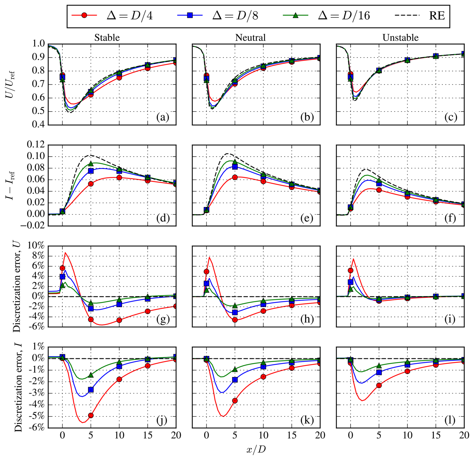
Figure C1 Influence of grid spacing on RANS-AD single-wake results in terms of rotor-averaged streamwise velocity (a–c) and wake-added TI (d–f) and corresponding discretization errors (g–l) for different stability cases. RE is Richardson-extrapolated value.