Multi-strategy wind farm control: alternating wake steering and helix wake mixing on a large-scale wind farm

Wind farm flow control mitigates wake effects by adjusting turbine settings to improve overall farm performance rather than the output of each turbine. Wake steering is an established wind farm flow control approach, while the helix method has recently emerged as a promising solution that enhances wake recovery by increasing mixing with the free-stream flow. This study quantifies the value of a combined strategy, in which each turbine can apply wake steering or the helix method. The analysis is performed considering different levels of uncertainty in wind direction, using engineering wake models that enable the simulation of these techniques on large-scale wind farms. A novel optimization algorithm, called multi-strategy serial-refine (MSR), is developed in this study, extending the state-of-the-art yaw-optimization method to include multiple control strategies and a generalized objective. A scaled version of an offshore wind farm in the Netherlands is selected as the case study, consisting of 69 IEA 22 MW turbines. The proposed combined strategy results in a greater increase in annual energy production than either individual strategy, leveraging the effectiveness of the helix method when multiple misaligned downstream turbines are present. This trend persists even under wind direction uncertainty. Due to the high sensitivity of wake steering to such uncertainty, the combined strategy benefits from the superior robustness of the helix method under these conditions.

1 Introduction

Wind farm flow control (WFFC) offers a promising solution to mitigate wake losses within a wind farm and enhance power production (Meyers et al., 2022). It consists of optimizing the performance of the entire farm collectively, in contrast to a greedy operation in which the power production of the turbines is maximized individually (van Wingerden et al., 2020). In recent years, different WFFC techniques have been developed. These can be divided into two main categories, namely quasi-static and dynamic WFFC (Meyers et al., 2022), where the latter are often referred to as active wake mixing techniques.

Among the quasi-static strategies, wake steering has emerged as the most effective solution (Doekemeijer et al., 2021). It consists of diverting the wakes from the downstream rotors by intentionally misaligning the turbines with the wind direction, hence using the yaw angle as a control variable. The efficacy of this technique has been widely demonstrated through large-eddy simulations (LESs), wind tunnel tests, and field experiments (Fleming et al., 2014; Gebraad et al., 2016; Campagnolo et al., 2020; Doekemeijer et al., 2021).

Conversely, dynamic WFFC techniques have not yet achieved a similar technological-readiness level. The underlying principle of these strategies is to enhance wake recovery through improved mixing with the surrounding free-stream flow, thereby increasing the energy extraction of the downstream turbines (Meyers et al., 2022). In recent years, various concepts have been explored to achieve this effect, collectively referred to as active wake mixing techniques. Munters and Meyers (2018) applied a sinusoidal signal to the thrust of the turbines, obtaining a pulsating wake. This method is referred to as dynamic induction control (DIC) or the pulse technique. Another promising technique, the helix approach, was proposed by Frederik et al. (2020), who achieved considerable power gains by applying individual pitch control signals to produce a helical wake shape. This concept has been proven through several LES studies (Taschner et al., 2023) and wind tunnel experiments (van der Hoek et al., 2024; Mühle et al., 2024), which have highlighted significant gains in power production but also increased structural loading on the turbines (Frederik and van Wingerden, 2022; van Vondelen et al., 2023).

Recent research has compared quasi-static and dynamic WFFC techniques through LESs, aiming to determine which solution yields higher power production under different inflow conditions and farm configurations. Taschner et al. (2024) have observed that the helix method is favorable with respect to wake steering only in the case of full wake overlap and up to six diameters of distance from the upstream turbine. However, they suggest that combining these methods could increase the robustness of the wind farm controller. This aspect is a consequence of the abrupt change in the yaw angle of the turbine that occurs at full alignment with the downstream turbine. Frederik et al. (2025) and Brown et al. (2025) have shown that wake steering exhibits higher performance than wake mixing methods, except for inflow conditions characterized by low veer. Therefore, these studies have shown that wake mixing techniques seem to outperform the more mature wake steering method only in limited scenarios. However, their analysis has been limited to the effects within a two-turbine array, and, therefore, these conclusions cannot be directly extended to large-scale wind farms. The main obstacle for the extension of such studies is the significant computational cost of multi-turbine LESs.

Large-scale wind farm simulations are usually performed using lower-fidelity steady-state wake models that provide a fast approximation of the wake characteristics. These are often referred to as engineering wake models. In recent years, a wide variety of these models have been proposed and implemented in the popular software tools FLORIS (National Renewable Energy Laboratory, 2024a) and PyWake (Pedersen et al., 2023). Specifically, wake deficit models are combined with wake deflection models, such as the model of Jimenez et al. (2010), to simulate the wind farm operation under yaw misalignment. Therefore, the low computational requirements of these models enable the optimization of the yaw angles for each turbine in large-scale wind farms, allowing the calculation of the increase in annual energy production (AEP) from wake steering. For instance, Simley et al. (2024) have applied these models to 15 different wind farms, calculating an AEP gain between 0.4 % and 1.7 % when wake steering is applied. Conversely, the literature lacks a comparable range of engineering models capable of simulating active wake mixing techniques. This is due not only to the lower technological-readiness level of these methods but also to the inherent difficulty of capturing their dynamic effects using steady-state models. Recently, an empirical Gaussian wake deficit and deflection model was added to the FLORIS tool (National Renewable Energy Laboratory, 2024a), which can simulate the effects of active wake mixing strategies by enhancing the wake recovery via a mixing factor. Dammann et al. (2025) have presented a model with similar capabilities using a super-Gaussian wake deficit model. Although these models enable broader comparisons and the potential integration of wake steering and active wake mixing, such a study has not yet been conducted on large-scale wind farms.

Another relevant aspect to consider when comparing and/or combining wake steering with active wake mixing is the uncertainty in the wind direction. This arises from different effects, such as the presence of turbulence and sensor errors (Quick et al., 2017), but also the spatial variation in wind direction in large wind farms, which is neglected by engineering wake models (von Brandis et al., 2023). Brown et al. (2025) have shown that wake mixing techniques outperform wake steering in the case of imperfect knowledge of the exact wake overlap position of the downstream turbine. However, the effect of such uncertainty on large-scale wind farms remains unclear for active wake mixing techniques. In contrast, this aspect has been studied extensively in the context of wake steering. Hodgson and Andersen (2026) demonstrated, through an LES study, that uncertainty in wind direction leads to a notable reduction in power gains. Quick et al. (2017) proposed an optimization under uncertainty to find the optimal yaw set points. Rott et al. (2018) have evaluated a control strategy that integrates wind direction uncertainty into yaw optimization using realistic time series. In this case, a Gaussian probability density function is used to model wind direction deviations, obtained by fitting real measurement data. Simley et al. (2020) have adopted a similar approach. The uncertainty in wind direction and the consequential unintentional yaw misalignments have also been considered in AEP calculations in recent studies (Quick et al., 2020; van der Hoek et al., 2020). In general, wake steering energy gains have been shown to drop significantly when uncertainties in input conditions are considered (van Beek et al., 2021). For instance, van der Hoek et al. (2020) have estimated an AEP gain between 0.34 % and 0.60 % considering a standard deviation in the wind direction of 3° for a 60-turbine wind farm. However, including such uncertainty in the yaw angle optimization problem can yield more robust AEP gains, thereby mitigating its detrimental effects.

Lastly, a critical aspect of applying WFFC in large-scale wind farms is selecting the optimization algorithm to determine the turbine control set points. General gradient-based methods available in the SciPy (Virtanen et al., 2020) or OpenMDAO (Gray et al., 2019) libraries can require substantial computational time as the number of turbines increases, since the problem dimensionality scales with the number of turbines. Fleming et al. (2022) have developed an algorithm for yaw angle optimization named serial-refine (SR). It is based on serial iterations from upstream to downstream turbines and represents a faster solution than traditional gradient-based methods. However, the SR algorithm has been developed specifically for wake steering; therefore, it cannot be directly applied when active wake mixing techniques are also considered.

In summary, previous studies have compared wake steering with active wake mixing techniques only for a limited number of turbines, while comparisons for large wind farms and the effects of a combined control strategy remain unexplored. This study addresses this problem by analyzing the effects of three different control methods: wake steering, the helix method, and a combined strategy that allows each turbine to apply either technique. It investigates the added value of adopting such a combined strategy for a large-scale wind farm, especially when wind direction uncertainty is present.

The main contributions of this work are outlined as follows:

• A comparison of different WFFC strategies in terms of potential AEP increase for a large-scale wind farm is provided.

• A sensitivity analysis with respect to different degrees of wind direction uncertainty is performed.

• A tailored algorithm for optimizing the control set points of a combined control strategy is developed, applicable to a generalized objective formulation.

• Trade-off solutions are investigated through a multi-objective optimization approach that incorporates a penalty on the control effort.

The remainder of this paper is structured as follows. Section 2 outlines the methodology adopted in this study. The results are then presented in Sect. 3 and discussed in Sect. 4. Lastly, the conclusion and recommendations for future research are included in Sect. 5.

2 Methodology

This section describes the methodology employed in this study, first explaining the wind farm model and the performance metrics selected as objectives. The optimization problem for determining the control strategies is then described, along with the optimization algorithm developed in this work. Lastly, the case studies chosen to showcase this framework are outlined.

2.1 Wind farm model

The turbines in the wind farm are modeled with their power and thrust curves. Dynamic effects are ignored, and it is assumed that a change in wind speed is instantaneously transmitted to the power production. The effect of wake steering on the actuating turbine is modeled by reducing the incoming wind speed by cos γ, with γ indicating the yaw misalignment. The power is then obtained from the corresponding power curve using the updated wind speed value. Similarly, the thrust coefficient C_T is also recalculated based on the updated wind speed value. However, it is further reduced by cos ²γ as defined by the simple yaw model implemented in the PyWake software (version 2.6.11) (Pedersen et al., 2023). The helix method is the strategy selected for this study among the different active wake mixing techniques. Consisting of a sinusoidal signal, the main control variables of this strategy are the excitation frequency, expressed through the Strouhal number St, and the blade pitch amplitude β (Frederik et al., 2020). The power P and thrust coefficient C_T are modeled as a function of their values during baseline operation, denoted by P_BL and C_T,BL, as

$$\begin{array}{}\text{(1)}& P\left(\mathit{\beta }\right)=P_{\mathrm{BL}}\cdot \left[\mathrm{1}-\left(b_{\mathrm{P}}+c_{\mathrm{P}}\cdot P_{\mathrm{BL}}\right)\cdot {\mathit{\beta }}^a\right],\end{array}$$

and

$$\begin{array}{}\text{(2)}& C_{\mathrm{T}}\left(\mathit{\beta }\right)=C_{\mathrm{T},\mathrm{BL}}\cdot \left[\mathrm{1}-\left(b_{\mathrm{T}}+c_{\mathrm{T}}\cdot C_{\mathrm{T},\mathrm{BL}}\right)\cdot {\mathit{\beta }}^a\right],\end{array}$$

where a, b_P, c_P, b_T, and c_T are coefficients that require proper tuning. In this study, the baseline operation is defined as the condition when WFFC is not applied. These equations follow the approach implemented in FLORIS (National Renewable Energy Laboratory, 2024a), where only the effect of a varying amplitude is considered, while St is assumed to be optimal.

The wake deficit model used in this study is the empirical Gaussian model implemented in FLORIS (National Renewable Energy Laboratory, 2024a), as it accounts for the added mixing induced by the helix control. The equations describing the model are included in Appendix A and available in the FLORIS documentation, where an extensive explanation is provided. A unique characteristic of this model is the introduction of the “wake-induced mixing factor”. This non-physical term is used instead of an explicit dependence on the turbulence intensity and is affected when the helix method is activated, enhancing the wake recovery depending on β. For consistency, the empirical Gaussian model is also adopted to determine the wake deflection caused by yaw or tilt misalignment. These models include several coefficients that have been tuned using high-fidelity simulations to match the conditions that characterize the site of the selected case study. A detailed description of this process is included in Appendix A. Both the wake deficit and deflection models have been integrated into the software PyWake to conduct this study.

The wake deficits caused by multiple turbines are added in quadrature while the inflow wind speed over the rotor a turbine is calculated through numerical integration, following the approach of Pedersen et al. (2022). These methods are directly available in PyWake, designated as Squared Sum and Gaussian Overlap, respectively.

2.2 Performance metrics

The AEP of the wind farm is selected as the main performance metric. To provide a realistic AEP estimate, the calculation accounts for uncertainty in wind direction. Specifically, this aspect is modeled by introducing deviations from each simulated wind direction, without adjusting the yaw angle of the turbines. This is achieved by including some offsets denoted by Δθ to the nominal wind direction, indicated with θ, and by weighting the power obtained for these multiple values of wind direction, θ+Δθ, using a probability distribution p_θ. In this case, a Gaussian function is used, defined by its standard deviation σ_θ and centered on the nominal wind direction. Then, the power P correspondent to a nominal flow condition (u,θ), with u indicating the wind speed, is obtained through the integration over the wind direction deviations, as indicated in Eq. (3). Based on this definition, σ_θ indicates both the variability in wind direction on timescales shorter than the control system reaction time and the uncertainty due to sensor errors. In the equation, f_P denotes the function that calculates the total power of the wind farm assuming $(u,\mathit{\theta }+\mathrm{\Delta }\mathit{\theta })$ as a free-stream flow condition. Specifically, f_P performs the summation of the power outputs of the individual turbines, which are calculated based on the turbine and wake models described previously. Each nominal flow condition (u,θ) is associated with different values of control variables, denoted by γ and β, which contain the yaw angles and helix amplitudes of each turbine. These are provided as input to f_P, affecting the power production of the wind farm. Since the yaw angles are defined relative to the input wind direction, which in this case is θ+Δθ, they are adjusted by adding Δθ before being provided as input to f_P, simulating the unintentional misalignment.

$$\begin{array}{}\text{(3)}& \begin{array}{rl}P(\mathit{\theta },u,\mathit{\gamma },\mathit{\beta },{\mathit{\sigma }}_{\mathit{\theta }})& =\int p_{\mathit{\theta }}(\mathrm{\Delta }\mathit{\theta },{\mathit{\sigma }}_{\mathit{\theta }})\\ & \cdot f_P(\mathit{\theta }+\mathrm{\Delta }\mathit{\theta },u,\mathit{\gamma }+\mathrm{\Delta }\mathit{\theta },\mathit{\beta })\mathrm{d}\mathrm{\Delta }\mathit{\theta }\end{array}\end{array}$$

Lastly, the AEP is calculated by integrating the power P over the different values of wind speed u and direction θ weighted by their probability of occurrence p(u,θ), as shown in Eq. (4). The term p(u,θ) is derived from Weibull distributions specified for each wind direction at each turbine location. The spatial variability in these distributions captures the heterogeneous wind resources across the wind farm. The arguments γ_LUT and β_LUT included in the equation refer to the lookup tables (LUTs) containing the values of γ and β for each flow case (u,θ).

$$\begin{array}{}\text{(4)}& \begin{array}{rl}\mathrm{AEP}({\mathit{\gamma }}_{\mathrm{LUT}},{\mathit{\beta }}_{\mathrm{LUT}})& =\mathrm{8760}\mathrm{h}{\mathrm{yr}}^{-\mathrm{1}}\cdot \iint p(u,\mathit{\theta })\\ & \cdot P(\mathit{\theta },u,\mathit{\gamma },\mathit{\beta },{\mathit{\sigma }}_{\mathit{\theta }})\mathrm{d}u\mathrm{d}\mathit{\theta }\end{array}\end{array}$$

To gain insights on the control effort experienced by the turbines during their yearly operation, another performance metric is introduced in this work, named control operation time and denoted by COT. It quantifies the period during which each turbine operates under a WFFC strategy, i.e., yawing or applying the helix method, and is defined as follows. First, the control effort of turbine i, denoted by c_E,i, is defined for each flow case as a binary variable that specifies whether the turbine i operates under a WFFC strategy:

$$\begin{array}{}\text{(5)}& c_{\mathrm{E},i}=\left\{\begin{array}{l}\mathrm{1}\text{ if }{\mathit{\gamma }}_i\ne \mathrm{0}\text{ or }{\mathit{\beta }}_i\ne \mathrm{0}\\ \mathrm{0}\text{ otherwise,}\end{array}\right.\end{array}$$

where γ_i and β_i are the yaw angle and the helix amplitude of turbine i, respectively, for the specific flow case. Second, the control operation time of turbine i, indicated by COT_i, which expresses the operation under a WFFC strategy in terms of percentage of its total operating time, is defined as

$$\begin{array}{}\text{(6)}& \begin{array}{rl}{\mathrm{COT}}_i({\mathit{\gamma }}_{\mathrm{LUT},i},{\mathit{\beta }}_{\mathrm{LUT},i})& =\mathrm{100}\cdot \iint p(u,\mathit{\theta })\\ & \cdot c_{\mathrm{E},i}({\mathit{\gamma }}_i,{\mathit{\beta }}_i)\mathrm{d}u\mathrm{d}\mathit{\theta },\end{array}\end{array}$$

where γ_LUT,i and β_LUT,i refer to the values of γ_LUT and β_LUT of turbine i. Lastly, the control operation time of the wind farm, denoted by COT, indicates the average control operation time between the different turbines and is hence defined as

$$\begin{array}{}\text{(7)}& \mathrm{COT}({\mathit{\gamma }}_{\mathrm{LUT}},{\mathit{\beta }}_{\mathrm{LUT}})={\displaystyle \frac{\mathrm{1}}{N_{\mathrm{wt}}}}\cdot \sum _{i=\mathrm{1}}^{N_{\mathrm{wt}}}{\mathrm{COT}}_i({\mathit{\gamma }}_{\mathrm{LUT},i},{\mathit{\beta }}_{\mathrm{LUT},i}).\end{array}$$

While a high COT can guarantee a larger AEP, it also increases the complexity of the control strategy, which may limit its practical feasibility or raise concerns about higher structural loads. This issue is particularly relevant for the helix technique, as its operation is often associated with increased loads on several critical wind turbine components (Frederik and van Wingerden, 2022).

2.3 Wind farm flow control optimization problem

The control set points of each WFFC control strategy are calculated by solving an optimization problem. The results are the optimal yaw angles and helix amplitudes for each turbine and flow condition, indicated by γ_LUT and β_LUT, respectively. This problem is divided into multiple sub-problems, each solved independently and referring to a different flow condition (u,θ). The design variables of each sub-problem are the yaw angles γ and the helix amplitudes β of the turbines in the farm for the given flow condition (u,θ). Their values are limited within the bounds [γ_min,γ_max] and [β_min,β_max]. In this study, each turbine operation is limited to either wake steering or the helix method, while different strategies are allowed across different turbines under the same flow conditions. This modeling choice is due to the lack of prior research and validation for cases in which wake steering and the helix method are implemented simultaneously on the same turbine.

In this work, two different optimization problems are solved, differing in their objective function. The first problem is defined in Eq. (8), whose objective is to maximize the power production P, which considers the effect of wind direction uncertainty.

$$\begin{array}{}\text{(8)}& \begin{array}{rlrl}{\displaystyle }\underset{\mathit{\gamma },\mathit{\beta }}{\text{maximize}}& {\displaystyle }& {\displaystyle }& {\displaystyle }P(\mathit{\theta },u,\mathit{\gamma },\mathit{\beta },{\mathit{\sigma }}_{\mathit{\theta }})\\ {\displaystyle }\text{subject to}& {\displaystyle }& {\displaystyle }& {\displaystyle }\mathit{\gamma }\in [{\mathit{\gamma }}_{\min },{\mathit{\gamma }}_{\max }]\\ {\displaystyle }& {\displaystyle }& {\displaystyle }& {\displaystyle }\mathit{\beta }\in [{\mathit{\beta }}_{\min },{\mathit{\beta }}_{\max }]\end{array}\end{array}$$

The second problem aims to maximize power production while minimizing control effort, hence adopting a multi-objective approach. The problem is described in Eq. (9), where the two objectives are combined through the weight w, which represents the relative importance of the two objectives.

$$\begin{array}{}\text{(9)}& \begin{array}{rlrl}{\displaystyle }\underset{\mathit{\gamma },\mathit{\beta }}{\text{maximize}}& {\displaystyle }& {\displaystyle }& {\displaystyle }P(\mathit{\theta },u,\mathit{\gamma },\mathit{\beta },{\mathit{\sigma }}_{\mathit{\theta }})-w\cdot {\sum }_{i=\mathrm{1}}^{N_{\mathrm{wt}}}{c}_{\mathrm{E},i}({\mathit{\gamma }}_i,{\mathit{\beta }}_i)\\ {\displaystyle }\text{subject to}& {\displaystyle }& {\displaystyle }& {\displaystyle }\mathit{\gamma }\in [{\mathit{\gamma }}_{\min },{\mathit{\gamma }}_{\max }]\\ {\displaystyle }& {\displaystyle }& {\displaystyle }& {\displaystyle }\mathit{\beta }\in [{\mathit{\beta }}_{\min },{\mathit{\beta }}_{\max }]\end{array}\end{array}$$

The problems described so far refer to the combined control strategy. In the case of individual wake steering and helix strategies, the corresponding optimization problems differ only by the definition of the design variables, which in the former case are limited to γ and in the latter to β.

2.4 Multi-strategy serial-refine (MSR) optimization algorithm

To solve the wind farm flow control optimization problems described in the previous section, a tailored optimization algorithm is developed, called multi-strategy serial-refine (MSR) optimization algorithm. The algorithm aims to find the control strategy for a wind farm that combines wake steering and the helix method to maximize a generic objective function. This algorithm extends the SR optimizer developed by Fleming et al. (2022). The design variables are extended to include several control strategies within a wind farm, rather than just wake steering. Furthermore, the algorithm is designed to allow an arbitrary user-defined objective function.

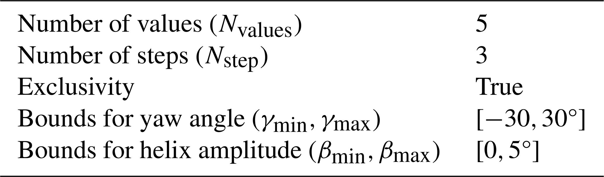
Analogous to the SR method, the MSR algorithm iterates over each turbine from the most upstream to the most downstream for each flow condition. At each iteration, a set of candidate control values is assessed for every turbine, and the best value is selected. The subsequent iteration is then initialized by perturbing the previously selected control variables with decreasing offsets, thereby refining the solution space. Therefore, the algorithm is characterized primarily by two hyperparameters: the total number of iterations, N_step, and the number of candidate values evaluated per turbine, N_values. The main distinction from SR is the procedure applied at each turbine iteration. In this extended version, multiple control strategies are tested in parallel, and the best-performing one is selected. The exclusivity of the control strategy is enforced at the perturbation step: for each turbine, if a perturbation is applied for a given strategy, the control set point for the other strategy is set to zero. This feature is enabled through the hyperparameter exclusivity.

The settings and hyperparameters of MSR adopted for this study are included in Table 1, while a more detailed description of the optimization algorithm can be found in Appendix B.

Table 1 Settings and hyperparameters of the MSR.

2.5 Case studies

Two case studies are considered to test the potential of a combined WFFC strategy. The first case study is a two-turbine wind farm in which the wind direction and speed are maintained constant at 270° and 8 m s⁻¹, respectively. Whereas the upstream turbine position is fixed, different downstream and cross-stream distances are tested for the second turbine. This simple example is used to provide an intuitive understanding of the model and algorithm used in this work. The second case study is a large-scale offshore wind farm consisting of 69 turbines. This is a scaled version of the Hollandse Kust Noord (HKN) wind farm, obtained by preserving the turbine spacing when normalized by their rotor diameter (D). The wind resources of the site are defined by the wind rose included in Fig. 1 and the heterogeneous wind speed field shown in Fig. 2 (Vortex FDC, 2024), which are scaled to the turbine hub height using a power law exponent equal to 0.1. Figure 2 also reports the layout of the wind farm. In this farm, the minimum distances between the turbines and the power density are 4.48 D and 6.03 W m⁻², respectively. For both case studies, the ambient turbulence intensity is set to 4 %, and the IEA 22 MW reference turbine (Zahle et al., 2024) is used, characterized by a diameter D of 283.2 m. The choice of this case study is motivated by the need to reflect current trends in future wind farm developments, which are characterized by rapidly increasing rotor sizes. Accordingly, the aim is not to provide a site-specific assessment of the proposed method for the HKN wind farm, but rather to draw conclusions that are representative of a generic large-scale offshore wind farm in the North Sea.

The computation of LUTs and the calculation of performance metrics require the discretization of the flow conditions. Specifically, the wind speed and directions are discretized into bins of 1 m s⁻¹ and 1°, respectively. In addition, a bin size of 1.25° is used to solve the integral related to the wind direction uncertainty, shown in Eq. (3), calculated within the interval $\left[-\mathrm{2}{\mathit{\sigma }}_{\mathit{\theta }},\mathrm{2}{\mathit{\sigma }}_{\mathit{\theta }}\right]$. Table 2 summarizes the main characteristics of the second case study.

In this work, three values of σ_θ are used to test the effectiveness of the WFFC strategies under various conditions: 0° (i.e., no uncertainty), 2.5°, and 5°. These choices are based on values reported in previous studies. For instance, Gaumond et al. (2014) obtained a σ_θ=2.67° from 10 min interval in the Horns Rev wind farm. Mittelmeier et al. (2017) extracted a σ_θ=3.6° from wind turbine sensor data. Quick et al. (2017) adopted σ_θ=5° in their work, and Rott et al. (2018) reported values around 5.25°.

In this study, the effects of different WFFC strategies are evaluated relative to a baseline case, defined as the condition in which all control variables in the LUTs are set to zero, corresponding to a greedy operation of the wind farm.

Table 2 Main characteristics of the scaled HKN case study.

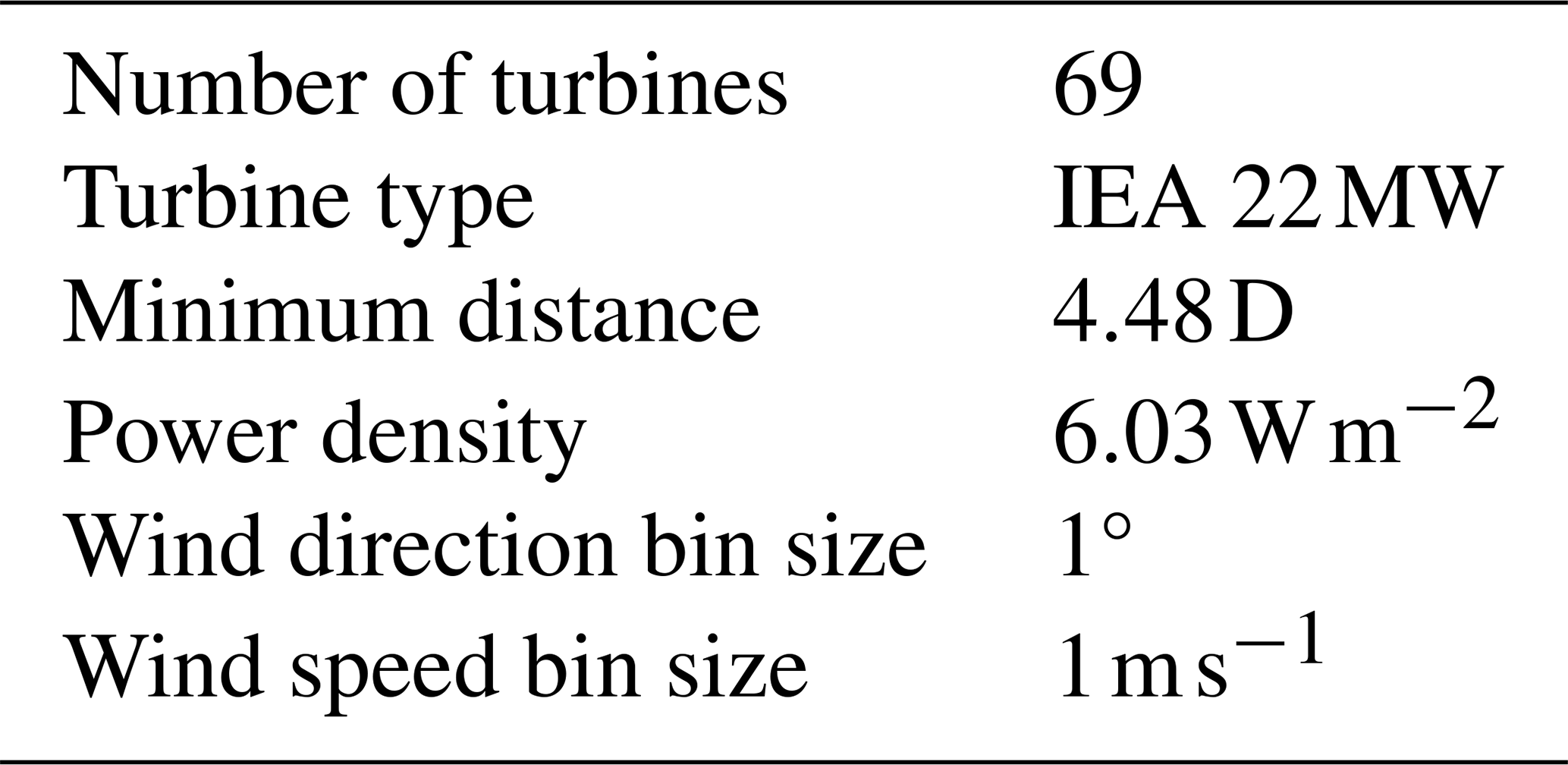
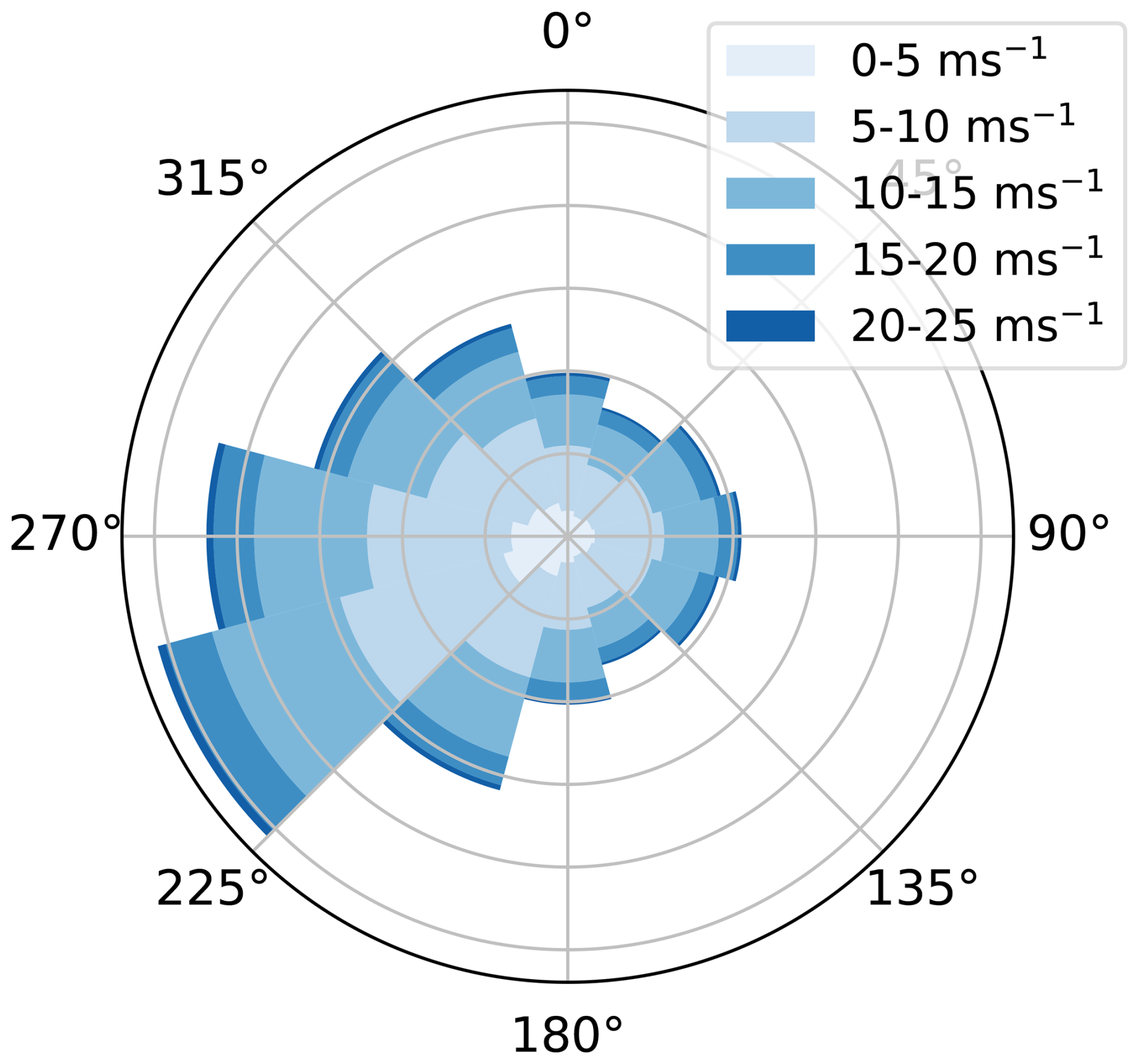
Figure 1 Wind rose of Hollandse Kust Noord site (Vortex FDC, 2024).

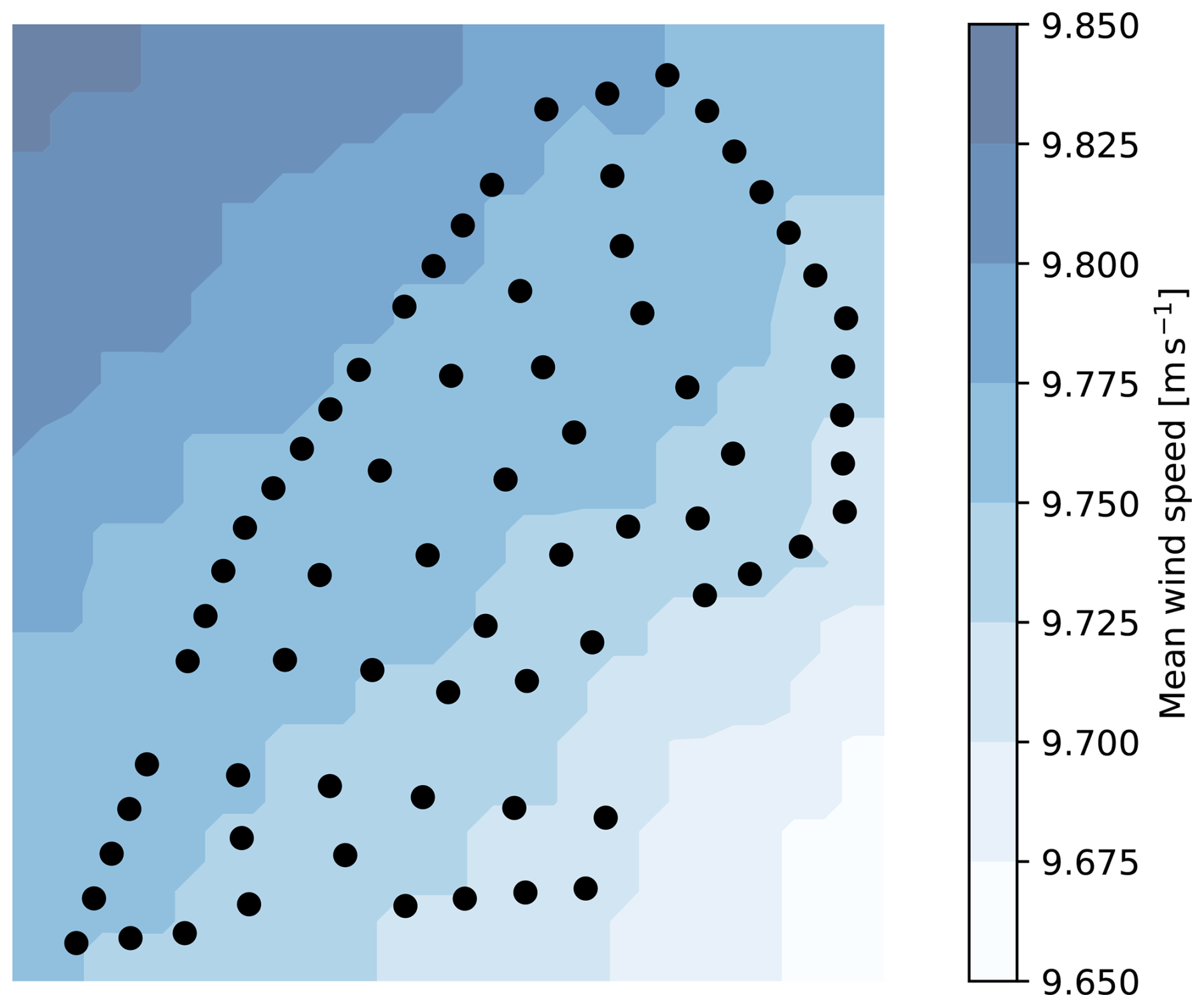
Figure 2 Location of the turbines and heterogeneous mean wind speed map at the Hollandse Kust Noord site.

3 Results

This section describes the results of the analysis conducted in this study. First, the engineering wake model used in this work is validated against LES data. Second, the capabilities of the combined control strategy are shown for the two-turbine example. Third, the results of the scaled HKN case study are presented in terms of an increase in AEP, the description of the optimal control variables, the impact on COT, and the trade-offs obtained with the multi-objective approach.

3.1 Model validation

This section compares the engineering wake model adopted in this study with LES data obtained under the same configuration. The specifications of the LES are detailed in Appendix A, specifically in Table A1.

Figure 3 Comparison between power gains obtained from the LES (second row) and the engineering wake model (third row) for a two-turbine wind farm. The control set point of the upstream turbine (shown in the first row) varies with the position of the downstream turbine, expressed in terms of streamwise and cross-stream distances from the upstream turbine, normalized with D. The wind speed and direction are 10 m s⁻¹ and 270°, respectively.

3.1.1 Validation of the wake deficit and deflection models

Figure 3 shows the power gains for a two-turbine wind farm, resulting from both the engineering wake model and the LES data. The first turbine is positioned at the origin of each plot, (0,0). The second turbine is placed at varying downstream and cross-stream distances, denoted by dx and dy, respectively. These distances are normalized by D and shown on the axes. A WFFC strategy is applied only on the first turbine, and its control set point varies depending on the position of the second turbine, as illustrated in Fig. 3. These control variables are chosen based on the insights described by Taschner et al. (2024).

The farm power gain values are computed as follows. First, the effective wind speed is obtained for the different downstream positions of the second turbine. These values are obtained through the wake deficit and deflection models mentioned in Sect. 2.1 and can be directly extracted from the LES. Second, the effective wind speed values are converted into rotor-average values using the same method for both the engineering wake model and the LES data, i.e., using the Gaussian Overlap mentioned in Sect. 2.1. This enables us to assess the accuracy of the wake deficit and deflection models, which have been re-tuned in this study, rather than the accuracy of the widely used rotor-average method available in PyWake, which has not been modified here. Lastly, these values are converted into power through the turbine model described in Sect. 2.1 for both cases. This final step assumes the presence of a virtual turbine in each of the downstream positions (dx,dy), following the method described by Vollmer et al. (2016).

It can be observed that the engineering wake model reproduces the LES results well in this simplified case, with only minor discrepancies. When wake steering is applied, the engineering wake model tends to underestimate the gains from wake steering. It cannot capture the mild spatial heterogeneity observed in LES when the helix method is simulated. These behaviors are also inherited by the combined strategy.

3.1.2 Validation of the overall power increase for a three-turbine array

In the previous section, the validation focuses exclusively on the wake models that were re-tuned for this study. In this section, we extend the analysis by comparing the full model toolchain adopted here with the results obtained from LES.

In this case, a three-turbine wind farm is studied with 4.5 D spacing between the three aligned turbines. Two different validation cases are considered, as described in Table 3. These cases differ in the wind direction, which is aligned with the turbine array in the first scenario and misaligned by 5° in the second scenario. This enables us to validate the model for both full and partial wake overlap conditions. For each case, both wake steering and helix operation are simulated, with the control set points included in Table 3.

Table 3 Three-turbine-array validation cases.

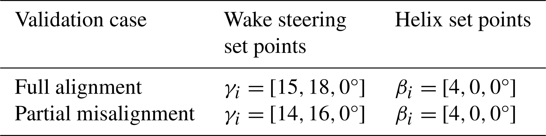
The results are shown in Fig. 4, where the power gains obtained from both the LES and the engineering wake model are plotted for each turbine and for the entire farm. The main trends observed in the LES results are reproduced by the engineering wake model; however, a moderate discrepancy can be observed in some cases.

A significant gap is evident between the total power gain when wake steering is applied for the full-alignment case. This is mainly due to a larger drop in power production from the actuating turbines. This aspect is related to the simple yaw model mentioned in Sect. 2.1 and used to simulate power reduction when turbines are yawing. However, this model has not been modified from its default implementation available in PyWake. This effect is also present for the partial misalignment case, for which the mismatch is less pronounced due to a more balanced spread in the power production between the three turbines.

When the helix method is simulated, the largest errors are observed for the first downstream turbines, i.e., T2. The discrepancy in power gain observed here does not match the results shown in Fig. 3, whose power values were calculated from the flow field instead of taken from the LES. This indicates that the mismatch is generated within the rotor-average process, for which the Gaussian Overlap model has not been modified from its default implementation available in PyWake.

Overall, even though these validation cases highlight a discrepancy between the engineering wake model and LES, the former always underestimates the power gains obtained through WFFC, demonstrating the conservative nature of this study.

Figure 4 Comparison between the power gains obtained from the LES and from the engineering wake model of a three-turbine array at 10 m s⁻¹. Left figure: full-alignment case. Right figure: partial-alignment case.

3.2 Two-turbine example

This section outlines the results for the case study consisting of two turbines. The optimal control variables of the front turbine are calculated for different positions of the downstream turbine and are shown in Fig. 5. These are obtained by solving the optimization problem depicted in Eq. (8), based on power maximization. As in the case shown in Fig. 3, the first turbine is positioned at the origin of each plot, and the second turbine is placed at varying downstream and cross-stream distances.

Nine cases are presented: the three WFFC strategies, wake steering, helix method, and combined for three values of uncertainty in wind direction, i.e., ${\mathit{\sigma }}_{\mathit{\theta }}\in [\mathrm{0},\mathrm{2.5},\mathrm{5}\mathit{°}]$. It can be observed that, as the uncertainty in wind direction increases, the downstream area for which the control is activated gets larger. However, the magnitude of the control variable diminishes, leading to a less aggressive strategy. This happens irrespective of the type of the WFFC strategy.

Analyzing the combined control strategy, for σ_θ=0°, there is only a very narrow region where the helix method is superior to wake steering. This condition only occurs in the case of perfect alignment between the two turbines and up to a limited distance, as also demonstrated by Taschner et al. (2024). Therefore, in this simplified example, if uncertainty in wind direction is neglected, a combined control strategy would not differ significantly from only using wake steering. However, as the uncertainty in the wind direction increases, the region where the helix method outperforms wake steering becomes larger, showing the added value of the combined strategy.

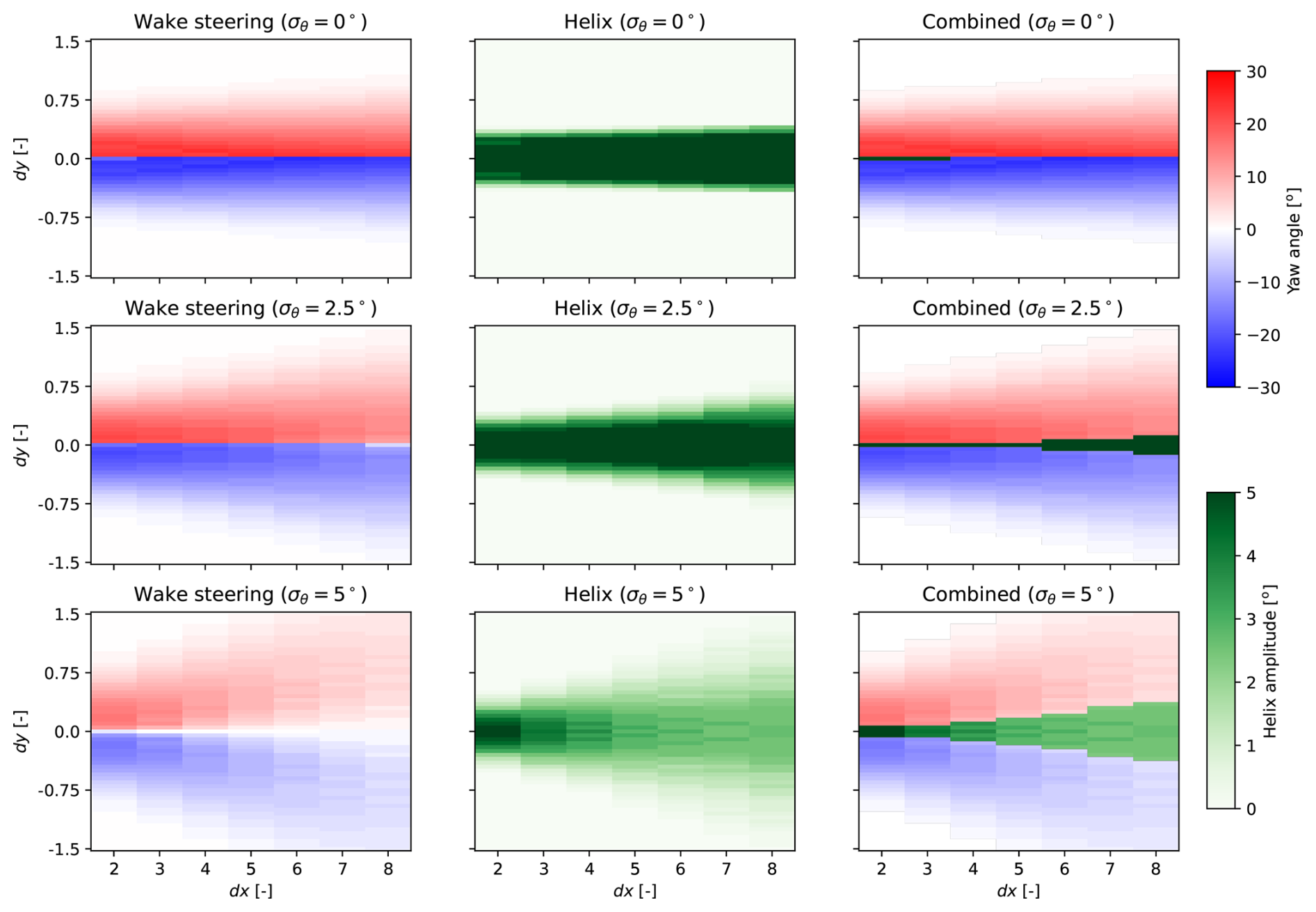
Figure 5 Optimal yaw angle and helix amplitude of the upstream turbine for different positions of the downstream turbine in a farm consisting of two turbines. The position of the downstream turbine is expressed in terms of streamwise and cross-stream distances from the upstream turbine, normalized with D. The wind speed and direction are 8 m s⁻¹ and 270°, respectively. Each subplot is characterized by a different control strategy and a different level of wind direction uncertainty, both specified in the subtitles.

Figure 6 shows the power gains corresponding to the optimal control strategy depicted in Fig. 5. These are defined as the percentage difference in wind farm power production between the case when WFFC is activated and the baseline operation. From Fig. 6, it can be observed that the power gains achieved through WFFC decrease as the uncertainty in wind direction increases. This detrimental effect appears to be more pronounced for wake steering than for the helix strategy. In most cases, the power gains from wake steering are higher than those achieved with the helix method. Furthermore, the plots for the combined control strategy closely resemble those obtained with wake steering alone. Overall, these results indicate that wake steering significantly outperforms the helix method in the partial-overlap case. Conversely, the helix method yields slightly higher power gains under fully aligned conditions; however, this difference remains marginal.

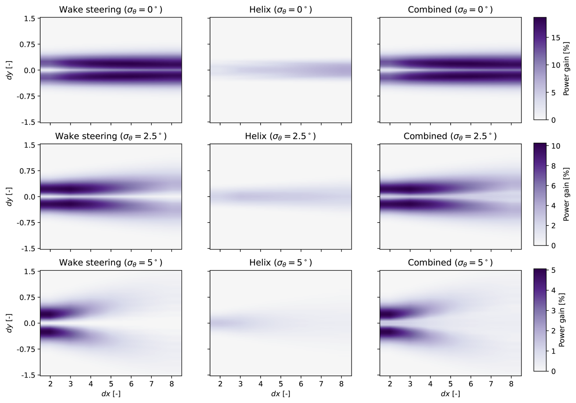
Figure 6 Power gains of the two-turbine wind farm for different positions of the downstream turbine. The wind speed and direction are 8 m s⁻¹ and 270°, respectively. Each subplot is characterized by a different control strategy and a different level of wind direction uncertainty, both specified in the subtitles.

3.3 Large-scale wind farm

This section outlines the results concerning the large-scale wind farm case study, for which the different WFFC strategies are applied to a scaled version of the HKN wind farm.

3.3.1 Increase in annual energy production

This section focuses on the impact of the combined strategy on the AEP of the wind farm. For this case study as well, the LUTs of optimal control variables are calculated to maximize the power production, as represented by Eq. (8). Different LUTs are obtained for three levels of wind direction uncertainty, namely ${\mathit{\sigma }}_{\mathit{\theta }}\in [\mathrm{0},\mathrm{2.5},\mathrm{5}\mathit{°}]$. The results presented in this section show increases in power production and AEP achieved by applying wake steering, the helix method, and the combined strategy.

Figure 7 shows the power gains of the wind farm for each control strategy as a function of the wind direction for a wind speed of 8 m s⁻¹. It can be observed that the magnitude of the power gains varies across the strategies, with the combined strategy showing the highest power gains for all cases. When the wind direction uncertainty is neglected (σ_θ=0°), Fig. 7 shows that wake steering provides higher gains with respect to the helix method, similarly to the two-turbine case study. As a consequence, wake steering is adopted by most of the turbines for the combined strategy as well. Therefore, the gains from the combined strategy are almost aligned with those from wake steering. However, a different behavior is observed as σ_θ increases. For σ_θ=2.5°, the situation is reversed; namely, the helix method outperforms wake steering. Therefore, the power increase provided by the combined control strategy is closer to the values obtained by the helix operation. This trend further increases when σ_θ=5°, for which the benefits of wake steering are significantly lower with respect to the helix method.

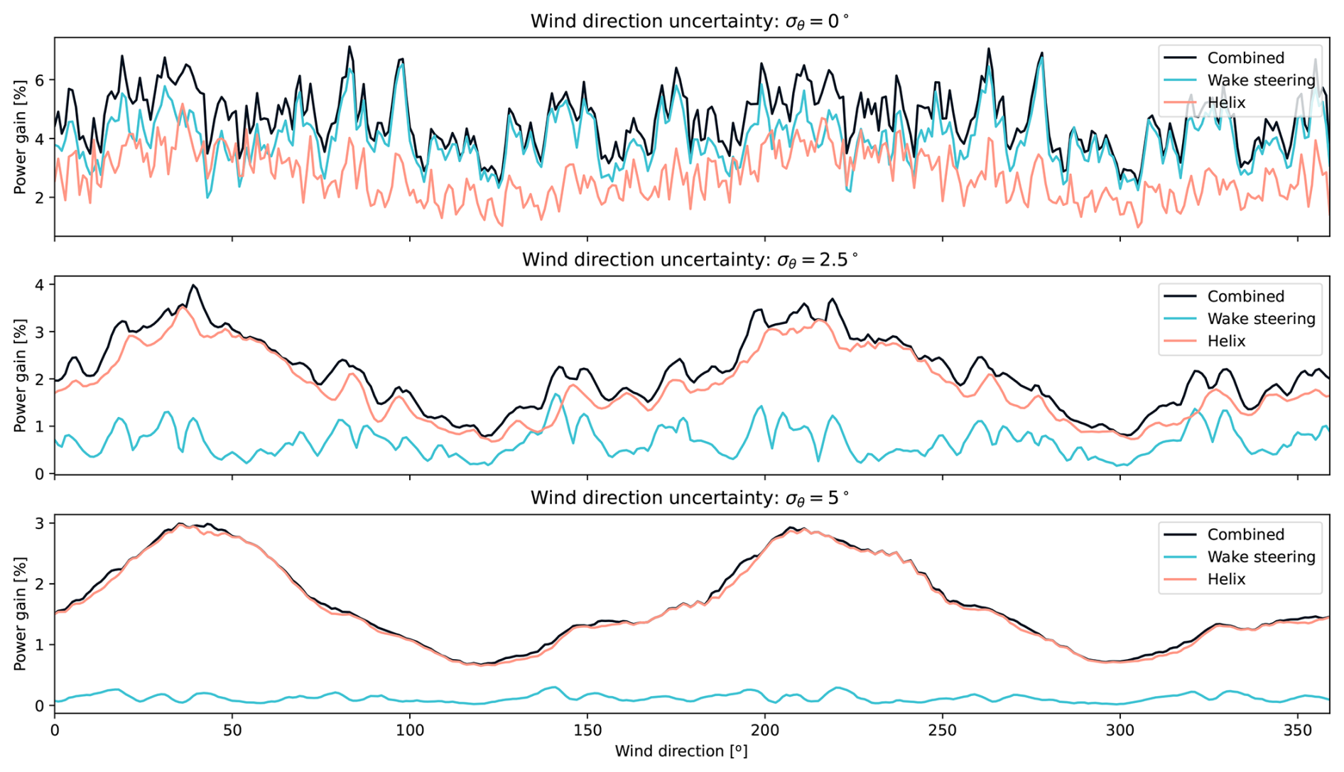
Figure 7 Power gains with respect to baseline operation of the scaled HKN wind farm for different wind directions. The figure includes different control strategies (indicated by different colors) and different degrees of uncertainty (specified in the subtitle of each plot). These values refer to a wind speed of 8 m s⁻¹.

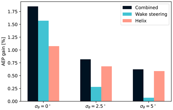
Lastly, to assess the performance of the different control strategies, the AEP values are calculated. Their values are expressed as percentage differences relative to the baseline operation, thereby providing a quantitative estimate of the benefits of the WFFC strategies over the lifetime of the wind farm. The results are reported in Fig. 8. As previously observed, wind direction uncertainty has a substantial unfavorable impact on the effectiveness of WFFC, regardless of the control strategy. This effect is highly pronounced for wake steering, where the AEP gain drops from 1.57 % to 0.28 % and 0.07 %, corresponding to values of σ_θ equal to 0, 2.5, and 5°, respectively. Conversely, Fig. 8 demonstrates that the AEP gains from the helix method are more robust with respect to wind direction uncertainty. Despite a lower AEP gain (1.07 %) for σ_θ=0°, it diminishes to 0.68 % and 0.59 %. Lastly, the combined strategy exhibits a high AEP gain (1.85 %) if σ_θ=0°, relying mostly on wake steering, while limiting the drop to 0.82 % and 0.62 % by exploiting the robustness of the helix method.

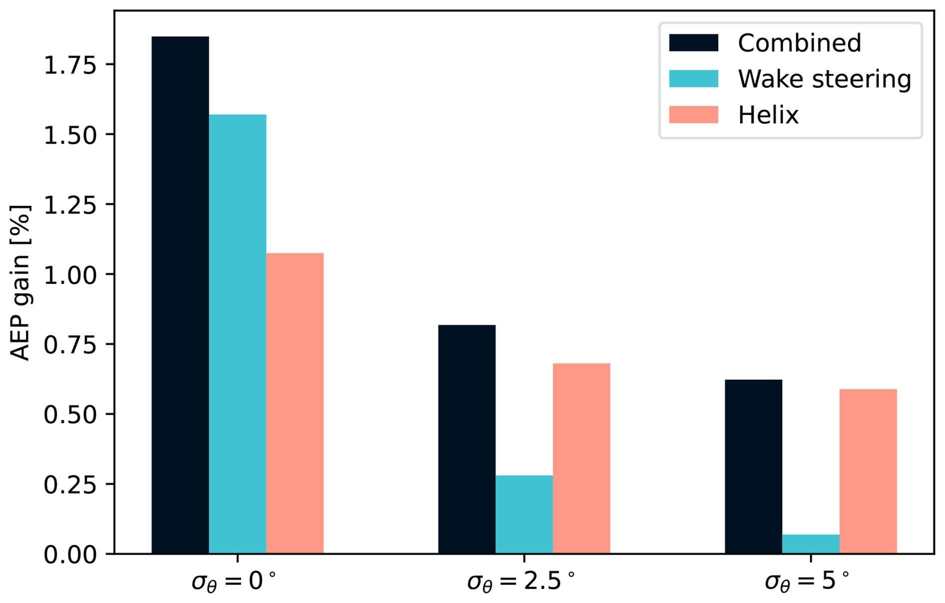
Figure 8 AEP gains with respect to baseline operation of the scaled HKN wind farm. The figure includes different control strategies (indicated by different colors) and different degrees of uncertainty (specified on the x axis).

Up to this point, the same values of σ_θ have been adopted for both the optimization of the control variables and the evaluation of the strategy, assuming perfect knowledge of the wind direction uncertainty. However, since in practice the values of σ_θ can be difficult to predict, this assumption is unlikely to be satisfied in reality. Therefore, a cross-comparison of the AEP gains obtained with different σ_θ used during optimization and evaluation enables us to assess the robustness of the different WFFC strategies under more realistic scenarios. These results are shown in Fig. 9. It can be observed that wake steering is highly affected by a mismatch between the σ_θ values. Overpredicting σ_θ significantly decreases the achievable AEP gains, while an underprediction even results in negative values. The helix strategy exhibits higher robustness with respect to an incorrect prediction of σ_θ, registering positive AEP gains for all the considered cases. Lastly, the robustness of the combined strategy lies between those of the two individual strategies.

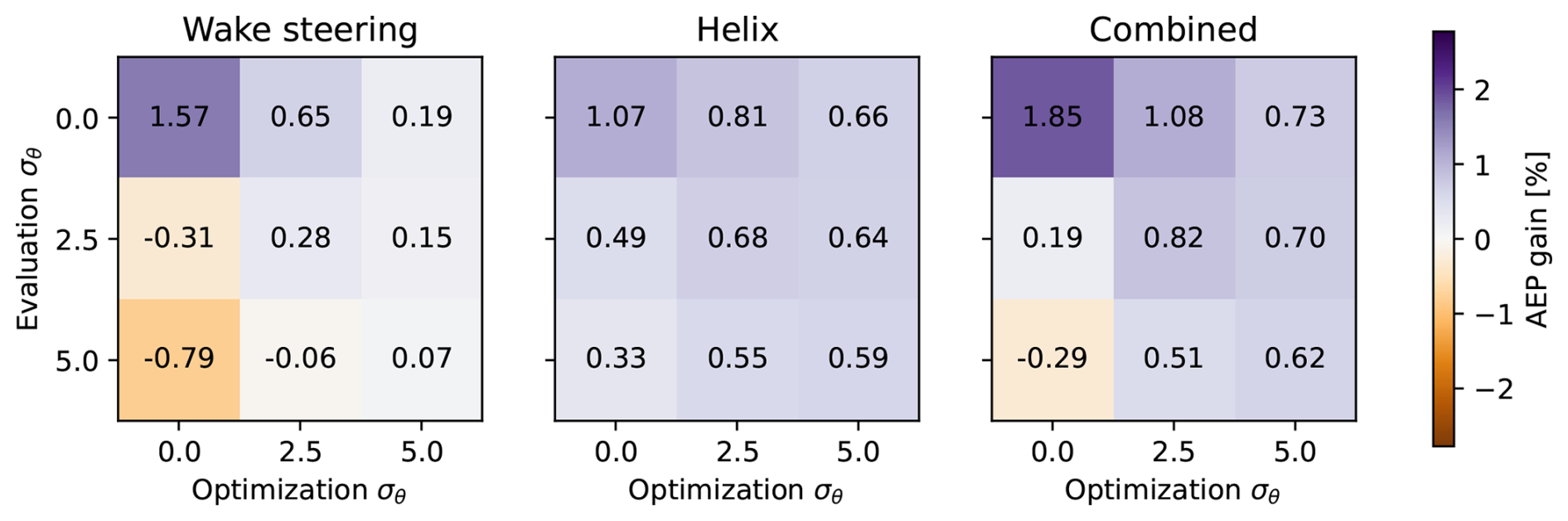
Figure 9 Cross-comparison of the AEP gains obtained for different σ_θ used for the optimization of the control variables and the evaluation of the strategy.

3.3.2 Lookup tables of the combined strategy

This section examines the control variables in the LUTs that yielded the power and AEP gains reported in the previous section. The plots show the optimal control settings required to achieve these gains, revealing general trends and evaluating the practical feasibility of implementing these control strategies. The results are shown for two representative cases: a turbine located at the farm boundary and one situated at its center. The optimal control values are depicted using a “control rose”, which displays the control variables as functions of wind speed and direction.

The left plot of Fig. 10 shows the control rose of one turbine in the front row facing the dominant wind direction, whose position is highlighted in the same figure. This refers to the LUTs of the combined control strategy, obtained for σ_θ=2.5°. It can be observed that this turbine applies wake steering only when the wind direction is oriented with the wind farm boundaries, where many turbines are aligned. Therefore, wake steering is activated only when the turbine can deviate its wake away from the majority of downstream turbines, and this condition cannot be achieved when the wake is facing the central region of the wind farm. Conversely, the helix operation is activated when the turbine wake impacts this region, where multiple turbines are present but not aligned in a single direction. This occurs because, rather than redirecting the wake toward other turbines, the wind speed deficit is reduced by enhanced mixing. Therefore, the two control strategies are used on this turbine to mitigate wake effects under different flow conditions, demonstrating that they complement each other well.

The right plot of Fig. 10 illustrates the control rose of a turbine that is placed in the central region of the wind farm. The results indicate that the control strategy of this turbine mainly consists of applying the helix technique, with wake steering being activated for a few limited cases. Specifically, it can be observed that the helix method is activated on this turbine for an even broader set of conditions with respect to the turbine located on the boundaries of the farm. The same explanation provided for the previous turbine still holds; i.e., helix control is favorable when multiple misaligned turbines are present in the wake. However, the aggressive control strategy of this turbine would probably not contribute significantly to the increase in AEP observed for the wind farm. This motivates a deeper analysis of the COT of the turbines, described in the next sections.

Figure 10 Control rose for the combined strategy of two different turbines. The exact position of the turbines is highlighted in the wind farm layout included in each subplot. Each subplot includes the values of the control variables in the LUT for each wind speed and direction, obtained with a wind direction uncertainty of σ_θ=2.5°. Left figure: turbine located at the boundaries of the farm. Right figure: turbine located in the central region of the farm.

3.3.3 Impact on the control operation time

This section investigates the impact of different control strategies on control operation time. Figure 11 reports the control operation time of each individual turbine, i.e., COT_i. The values are shown using boxplots, which summarize the main trends across the turbines for each condition. It can be observed that the values of COT_i can differ significantly depending on the turbine, as highlighted by the vertical length of each “box”. Moreover, different values of COT_i are obtained depending on both the control strategy and the level of uncertainty. However, the main observation from Fig. 11 is that some turbines would operate under either wake steering or helix mode for more than 60 % of the time. In the case of the helix method, this could lead to a significant increase in structural loading, rendering the control strategy infeasible. These results can be explained based on the problem statement in Eq. (8), where the use of control is not penalized. As a result, the use of WFFC is encouraged even if only a minimal gain in power production is obtained. Moreover, two additional aspects can be observed in Fig. 11. First, the effect of wind direction uncertainty on COT_i depends on the control strategy. Figure 11 highlights a direct correlation with σ_θ for the helix method and the combined strategy, while an inverse trend is observed for wake steering. Second, the values of COT_i related to the helix method and the combined strategy are significantly higher than for wake steering when uncertainty in wind direction is considered. An explanation to this result can be provided by assuming that several turbines present a LUT similar to the one depicted in the right plot of Fig. 10. In this case, the turbines use either wake steering or the helix method for most flow conditions below the rated wind speed, which represent a significant fraction of total operating time.

Figure 11 Control operation time for different control strategies (indicated by the color) and wind direction uncertainty (specified on the x axis ). Each boxplot summarizes the values of all the turbines in the wind farm for the specific condition.

3.3.4 Multi-objective

A multi-objective approach is used to balance the gains in power production from the different control strategies and their associated control effort, as described in Eq. (9). The results are shown in Fig. 12, where the effect of different LUTs is included in terms of AEP gain and COT. Each data point on the Pareto front corresponds to a different LUT, with its associated performance metrics. The different values that determine each curve are obtained by increasing the penalty weight on the control effort in the objective function. Specifically, the Pareto fronts have been obtained by varying the weight w from 0 to 10⁶. The results are shown for the three different control options investigated in this study, assuming σ_θ=2.5°. Moreover, two additional cases have been included, where β_max in the helix method and the combined strategies has been limited to 2.5°, in contrast to the value of 5° adopted in the rest of the study. This provides a wider overview of the potential of these techniques, quantifying the impact of a less aggressive helix operation, for instance, due to constraints on the structural loads (Frederik and van Wingerden, 2022; van Vondelen et al., 2023).

All the Pareto fronts represented in Fig. 12 show the presence of a trade-off between AEP and COT. The AEP gains are higher for the combined strategy than for the individual strategies, consistent with previous results. However, the steepness of the Pareto fronts in proximity to the largest AEP gains indicates that beneficial trade-offs can be achieved. For instance, the COT of the combined strategy can be limited to 21.4 % while keeping the AEP gain equal to 0.74 %, obtained for w=10⁵. When β_max is limited to 2.5°, a shift in the Pareto curve is observed. In this case, a combined control strategy that aims for a favorable trade-off between the two objectives can increase the AEP by 0.61 % while keeping COT to 20.2 %. Similar trends can also be observed for wake steering and the helix method. Overall, this analysis shows that a significant reduction in the COT can be achieved at the expense of only a marginal decrease in the AEP gain and that even in this case, the combined strategy outperforms the individual techniques.

Figure 12 Trade-off between AEP gains and COT for wake steering, the helix method, and the combined strategy and for a maximum helix amplitude β_max of 5 and 2.5°. The results refer to a wind direction uncertainty of 2.5°.

4 Discussion

This section provides a more detailed interpretation of the results obtained in this study, highlighting both their significance and limitations.

4.1 Insights on the comparison between different strategies

The comparison between wake steering and the helix method has proven the superiority of the former when perfect inflow knowledge is used. However, the latter becomes more favorable when uncertainty in wind direction is introduced, i.e., when more realistic conditions are simulated. This is a consequence of the asymmetric profile of optimal yaw angles with respect to the direction of full alignment with the downstream turbine, which constitutes a point of discontinuity. In the proximity of this condition, the optimal yaw angles switch from positive to negative large values, as clearly shown in Fig. 5. Therefore, in the absence of a well-defined misalignment direction, wake steering may be detrimental to power production. Conversely, such behavior is not present for the helix operation, where a symmetric profile is observed.

This effect is amplified as the size of the wind farm increases. In many cases, having multiple downstream turbines prevents the upstream turbine to effectively steer the wake away from them. This condition occurs when the wake of the upstream turbine affects the central region of the farm, whereas wake steering remains extremely fruitful when the upstream turbine redirects the wake outside the entire farm. In contrast, the helix technique does not exhibit this effect, as it reduces the wind speed deficit rather than displacing it. Therefore, the advantages of the helix approach become clearer when a large-scale wind farm is considered rather than a limited number of turbines. These insights are expected to hold for wind farms with a similar number of turbines, layout, and power density to our case study; however, these trends may vary across other types of wind farms.

In this study, the helix technique is chosen as the active wake mixing strategy. However, the same framework can be used to study the impact of other techniques such as the pulse method, for which Frederik et al. (2025) have demonstrated superior performance for some flow cases. This would only involve minor changes in the turbine model and the re-tuning of some coefficients that characterize the wake model. However, since the steady‐state effects are expected to be similar to those observed for the helix method, similar trends are also expected irrespective of the specific active wake mixing technique employed.

4.2 Reliability of low-fidelity wind farm models

The magnitude of the AEP gains reported in this study is highly dependent on the low-fidelity models used, especially their coefficients. For instance, the power–yaw loss exponent, which is often used to estimate the drop in power production under yaw misalignment (Liew et al., 2020), can significantly affect the effectiveness of wake steering and its integration into the combined strategy. In this study, the default method in PyWake is used based on the cosine-loss law to recalculate the effective wind speed and the extraction of the updated power from the power curve using this wind speed value. In our case, this results in a power–yaw loss exponent between 2.5 and 3.1, depending on the wind speed. Conversely, Liew et al. (2020) have proven that the actual power–yaw loss exponent can be lower. Consequently, reducing this value would lead to higher power gains for wake steering. As a result, wake steering would be adopted for a higher number of cases within the combined strategy, increasing the overall AEP gain. However, this would not affect the general trends presented in this work.

The coefficients adopted for these models have been tuned through aeroelastic simulations and LES to replicate the conditions of a realistic site. However, due to the significant computational resources required for LES, this study considers only a limited set of conditions for the model calibration and validation. These are restricted to a single atmospheric boundary layer condition and to a fixed value of the free-stream wind speed and the turbulence intensity. More importantly, the analysis is limited to configurations with up to three turbines at fixed spacing. An example of these limitations is the synchronization concept for the helix operation in multiple turbines. In this regard, recent studies have highlighted that synchronizing the wake dynamics of multiple turbines using the helix method may affect the power production significantly (van Vondelen et al., 2025). As of now, this aspect is not considered by the available low-fidelity models, including the model used in this study. The impact of this assumption is analyzed in Sect. C1.

Another limitation is that the operation of the WFFC strategies is not explicitly constrained to the below-rated region, where they are typically tested or simulated using higher-fidelity models. However, as shown in the LUTs in Fig. 10, this operation occurs only in a limited number of cases. Moreover, for the helix method, it has been verified that this assumption yields negligible differences compared to the presented results.

In conclusion, the application of the engineering wake model in this study extends beyond the conditions for which it has been originally tuned. This may lead to some uncertainty in the reported AEP gains obtained with this method; however, we do not expect this to affect the main trends observed in the present work. To increase the reliability of results from WFFC on large-scale wind farms, the scale of the LES used for validation should be extended from a few turbines to larger wind farms to investigate deep-array effects and avoid extrapolation beyond the validated conditions. Lastly, since LES is a numerical modeling approach, experimental field data are essential to improve the reliability of low-fidelity models in representing wake mixing effects and to validate the effectiveness of active wake mixing strategies on large-scale wind farms.

4.3 Implications of estimating the AEP using LUTs

In this study, the benefits of the different control strategies are estimated using LUTs, which contain the optimal control variables for each specific flow condition. Such estimation is typically performed under the assumption of perfect knowledge of the wind direction (σ_θ=0), thereby simulating the exact flow conditions for which the control variables in the LUTs were derived. Such assumptions could lead to an overestimation of the AEP gains provided by the control strategies, due to the dynamic inflow conditions under which the turbines operate. Specifically, this assumption would require the control settings to be continuously updated to match the values in the LUTs. In this work, the assumption is relaxed by increasing σ_θ, thereby simulating more realistic conditions.

The use of LUTs for estimating the AEP does not imply that they are employed in the actual operation of the wind farm. In the context of AEP estimation, the LUTs assume that the operator applies the optimal control variables under each flow condition defined by u and θ, subject to an error margin determined by the wind direction uncertainty. However, the manner in which these control settings are implemented in response to dynamic flow conditions does not need to match the way the AEP is calculated to maintain the validity of the estimation. For instance, the control set points may be applied through a combination of LUTs and a low-pass filter or via more advanced closed-loop control strategies (Becker et al., 2025b).

In this context, the interpretation of the wind direction uncertainty is twofold. First, it estimates the impact of undesired effects such as sensor errors or rapid changes in wind conditions. Second, it reflects the behavior of a control approach designed to minimize actuator interventions, maintaining unaltered the control settings across a wider range of inflow conditions (Becker et al., 2025a).

While the decoupling between AEP estimation and the implementation of the actual operational strategy ensures the broad applicability of the proposed method, it also raises concerns regarding the practical feasibility of deploying the combined control strategy. As previously noted, this strategy entails certain turbines operating under wake steering, while others use the helix technique, with neither method applied simultaneously to a single turbine. This study has highlighted that switching between these two strategies for different inflow conditions can lead to a substantial increase in power production. However, how this transition can be executed during actual operation remains unexplored and requires validation through LES and wind tunnel experiments. Lastly, the performance of the helix method under yaw misalignment remains largely unexplored, yet it may offer further AEP improvements and thus merits detailed investigation.

4.4 Impact of the flow characteristics

In this work, the flow characteristics have been selected to replicate the site conditions of the case study. However, Frederik et al. (2025) have shown that the veer has a significant impact on selecting the best control strategy. Therefore, a sensitivity analysis of the veer value would provide a wider overview of the comparison between the different control options tested in this study.

The turbulence intensity is also expected to play a major role in comparing and combining different WFFC techniques. In this study, the LES data used to tune the engineering wake model were run with an ambient TI of 4 %, which lies toward the lower bound of the typical range of 4 %–6 % observed in the North Sea (Türk and Emeis, 2010). Lower TI is generally associated with larger wake deficits and slower wake recovery. Consequently, this may lead to an overestimation of the AEP gains achieved by WFFC strategies, as higher TI regimes would reduce their effectiveness. As an example, Dammann et al. (2026b) report that, for a two-turbine setup, the power uplift achieved with the helix method decreases from 18 % to 2 %–4 % as the turbulence intensity increases from 2.0 % to 13.1 %.

Moreover, the empirical Gaussian wake model adopted in this study does not explicitly depend on such parameters, relying solely on the tuning process. Therefore, the model coefficients would need to be re-tuned for each investigated turbulence intensity, requiring an extensive dataset of LESs that cover all these conditions. Therefore, a wake model for active wake mixing with a direct dependence on turbulence intensity, such as that recently published by Dammann et al. (2026a), would facilitate this analysis.

After completing all these sensitivity studies, multi-dimensional LUTs can be obtained by applying the framework developed in this work, in which the optimal control variables are selected for all possible combinations of flow parameters.

4.5 Towards a value-centered wind farm flow control

The framework and the algorithm developed in this study have been designed to ensure high flexibility in the objective function used to determine the optimal control strategy. Therefore, the optimization of the WFFC strategy can be extended beyond the traditional power production, exploring different value-based metrics (Meyers et al., 2022).

In this study, this concept has been demonstrated by balancing annual energy production with control operation time. In the case of the helix operation, this variable can be directly related to an increased structural loading (Frederik and van Wingerden, 2022), while for wake steering, the relation between these two aspects is more complex. A first attempt to better capture the information about the increased loads can be to penalize the control operation depending on the effective wind speed value and the magnitude of the control variable, i.e., yaw angle and helix amplitude values. Alternatively, load surrogate models can be integrated in this framework to provide better results with respect to power-load trade-off strategies. For instance, Guilloré et al. (2024) proposed a surrogate model based on an artificial neural network that enables a rapid load estimation, while Anand et al. (2025) adopted this model to demonstrate the use of WFFC including lifetime-aware considerations. However, this model does not yet support active wake mixing control strategies.

Although most of this work has focused on maximizing the power production, the main objective could be shifted to the revenues generated by the wind farm using the same method and algorithm. This is expected to further increase the benefits of WFFC when wind speed and electricity prices are negatively correlated (Bechmann and Quick, 2025). This is a consequence of the fact that WFFC is mostly applied in the below-rated region, i.e., for low values of wind speed that are often associated with higher electricity prices.

Lastly, the proposed methodology and the developed algorithms can be applied to study the impact of WFFC beyond commercial metrics, including environmental, ecological, and/or social objectives within the wind farm flow control optimization problem (Meyers et al., 2022; Kainz et al., 2025).

5 Conclusions

This study has analyzed the added value of a wind farm flow control strategy that combines wake steering with the helix active wake mixing method. This combined strategy has demonstrated a substantial increase in the power production of large-scale wind farms, achieving AEP gains higher than those obtained individually for wake steering and the helix method.

When the number of turbines is limited, and perfect knowledge of wind direction is assumed, wake steering has been shown to outperform the helix method in terms of power gains. However, as wind direction uncertainty increases, helix control has been shown to be more robust, exhibiting smaller reductions in power gain than wake steering. Moreover, as the number of turbines increases, the helix method has shown greater effectiveness in reducing wake losses in scenarios with multiple downstream turbines. This can be explained by the fact that when a turbine applies wake steering, redirecting the wake away from the nearest downstream turbine may inadvertently deflect it toward other turbines further downstream.

Overall, the combined strategy has achieved the largest power increase by leveraging the complementary benefits of the individual strategies. This outcome stems from the high gains provided by wake steering under specific favorable conditions, the greater robustness of the helix method with respect to wind direction uncertainty, and its effectiveness when multiple misaligned downstream turbines are present. However, such performance would require some turbines to operate under a WFFC strategy up to 60 % of their operation time, raising concerns about its actual feasibility. A multi-objective approach that balances the control effort with increased power production has been adopted for optimizing the control variables. This has enabled us to find a strategy that limits control actuation while still ensuring a significant power increase. This analysis has been enabled by the development of a tailored algorithm, MSR, designed to provide high flexibility to the user, in terms of both control strategies and optimization objectives.

However, these results are based on recent wake models used for wind farm simulation, which are associated with notable uncertainties, as they are applied beyond the range of conditions for which they have been validated. Future research could reduce such uncertainty by extending validation of the engineering models for active wake mixing, performing LES for large-scale wind farms, performing wind tunnel tests, and conducting field experiments. Moreover, a wider range of flow conditions could be simulated, providing comprehensive lookup tables of optimal control settings that also depend on parameters such as turbulence intensity or veer. Lastly, the full potential of this framework could be exploited by extending the analysis to the combination of more control strategies, e.g., including turbine derating, and more objectives, for instance, related to structural, financial, environmental, ecological, and/or social aspects.

Appendix A: Description and tuning of the turbine and wake models

This appendix provides descriptions of the empirical Gaussian wake deficit and deflection models, as well as the tuning procedure for the turbine and wake models.

A1 Description of the empirical Gaussian model

The empirical Gaussian model adopted in this study is extensively described in FLORIS documentation (National Renewable Energy Laboratory, 2024a); however, the main equations are reported here as well.

Table A1 LES settings adopted for the tuning process.

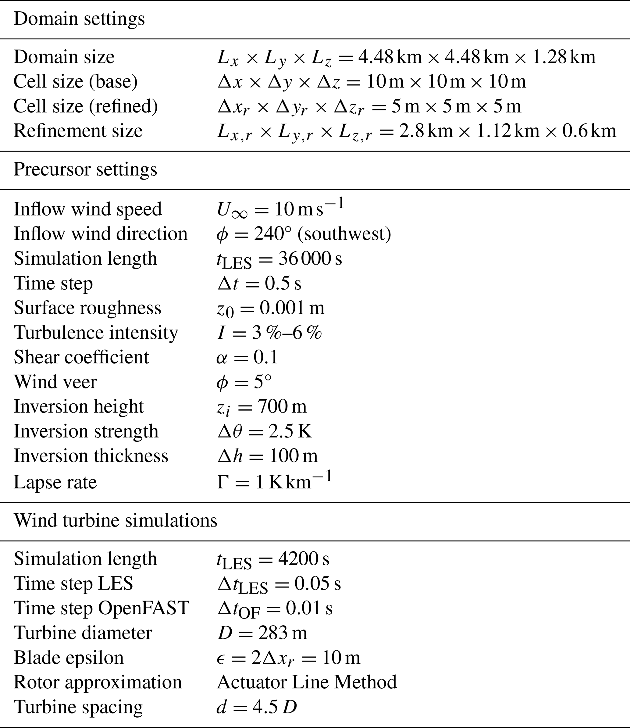
Table A2 LES cases adopted for the tuning process, specifying the number of turbines (N_WT), control settings (γ,β), and whether they were used for tuning the turbine or the wake model.

Table A3 Tuning coefficients of turbine and wake models.

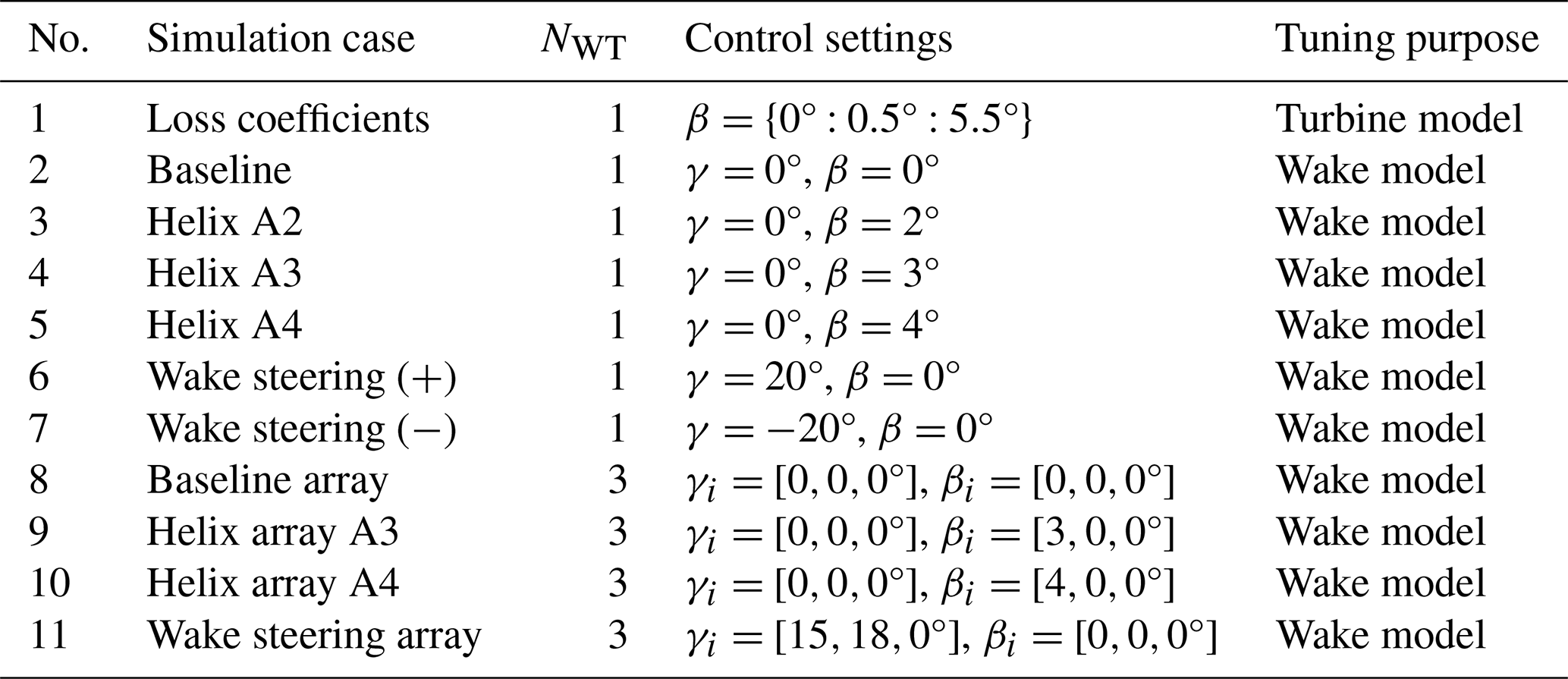
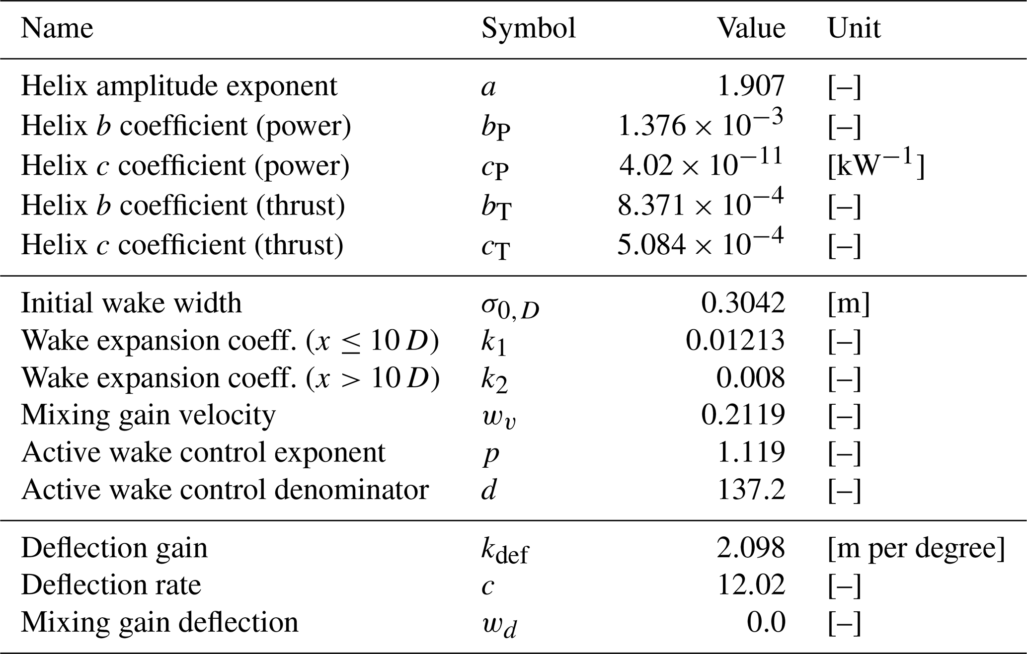
Figure A1 Comparison between the tuned turbine model and the OpenFAST/LES data for both power loss and thrust loss for different helix amplitudes. The functions obtained with the default coefficients available in FLORIS are also included.

The normalized wind speed at the point $(x,y,z)$ is expressed as

$$\begin{array}{}\text{(A1)}& {\displaystyle \frac{u}{U_{\mathrm{\infty }}}}=\mathrm{1}-C\cdot \exp \left[-{\displaystyle \frac{(y-{\mathit{\delta }}_y{)}^{\mathrm{2}}}{\mathrm{2}{\mathit{\sigma }}_y^{\mathrm{2}}}}-{\displaystyle \frac{(z-{\mathit{\delta }}_z{)}^{\mathrm{2}}}{\mathrm{2}{\mathit{\sigma }}_z^{\mathrm{2}}}}\right],\end{array}$$

where the scaling factor C of the Gaussian curve and the lateral wake width σ_y depend on the downstream position x of the point at which the wind speed is evaluated and are modeled as

$$\begin{array}{}\text{(A2)}& C={\displaystyle \frac{\mathrm{1}}{{\mathit{\sigma }}_{\mathrm{0},D}^{\mathrm{2}}}}\cdot \left(\mathrm{1}-\sqrt{\mathrm{1}-{\displaystyle \frac{{\mathit{\sigma }}_{y,\mathrm{0}}{\mathit{\sigma }}_{z,\mathrm{0}}{C}_{\mathrm{T}}}{{\mathit{\sigma }}_y{\mathit{\sigma }}_z}}}\right)\end{array}$$

and

$$\begin{array}{}\text{(A3)}& \begin{array}{rl}{\mathit{\sigma }}_y\left(x\right)& ={\mathit{\sigma }}_{y,\mathrm{0}}\\ & +\underset{\mathrm{0}}{\overset{x}{\int }}\left[\sum _{i=\mathrm{0}}^n{k}_i\cdot l_{[b_i,b_{i+\mathrm{1}})}\left(x^{\prime }\right)+w_v\cdot M_j\left(x^{\prime }\right)\right]\mathrm{d}{x}^{\prime },\end{array}\end{array}$$

respectively. The vertical wake width σ_z is defined similarly to σ_y, hence following Eq. (A3). δ_y and δ_z indicate the lateral and horizontal wake deflection, respectively, and depend on the downstream position x. C_T indicates the thrust coefficient, whereas σ_0,y and σ_z,0 represent the initial wake widths at the turbine location. A feature of this model is the use of multiple wake expansion coefficients k_i at different downstream positions defined by the breakpoints b_i. The transition between different k_i values is smoothed using the function l.

The wake-induced mixing factor M is modeled as

$$\begin{array}{}\text{(A4)}& M_j=\sum _{i\in T^{\mathrm{up}}\left(j\right)}{\displaystyle \frac{A_{ij}{a}_i}{\frac{x_j-x_i}{D}}}+{\displaystyle \frac{{\mathit{\beta }}^p}{d}},\end{array}$$

dependent on the induction factor a and the area overlap A between turbine wakes and their relative downstream distances normalized with the rotor diameter D, but also on the helix amplitude β and the tunable coefficients p and d. Yaw-added mixing is neglected in this study.

Lastly, the wake deflection caused by the yaw misalignment γ is modeled as

$$\begin{array}{}\text{(A5)}& {\mathit{\delta }}_y={\displaystyle \frac{k_{\mathrm{def}}\cdot C_{\mathrm{T}}\cdot \mathit{\gamma }}{\mathrm{1}+w_d\cdot M_j}}\ln \left({\displaystyle \frac{\frac{x}{D}-c}{\frac{x}{D}+c}}\right),\end{array}$$

with k_def, w_d, and c indicating tunable coefficients.

Figure A2 Wind speed deficit modeled using the empirical Gaussian model and LES data, considering no control (“baseline”), wake steering, and helix control, shown for downstream distances of 4, 6, and 8 D. The plots refer to one-turbine simulations.

Figure A3 Wind speed deficit modeled using the empirical Gaussian model and LES data, considering no control (“baseline”), wake steering, and helix control, shown for downstream distances of 7, 8.5, and 11.5 D. The plots refer to the simulations of three aligned turbines, with a spacing of 4.5 D.

A2 Tuning of the turbine and wake models

This section describes the tuning process used to determine the coefficients present in the turbine and wake models.

The tuning procedure is based on a dataset obtained through multiple simulations performed with the LES solver AMR-Wind (Kuhn et al., 2025), which has been coupled with the aeroelastic simulator OpenFAST (National Renewable Energy Laboratory, 2024b) to model a wind turbine's response. The simulations were run with a conventionally neutral boundary layer at turbulence levels similar to those observed in the North Sea. Multiple cases were simulated, covering different control strategies and layouts. An overview of the LES settings and the simulation cases is provided in Tables A1 and A2.

The tuning process has been decomposed into six sequential steps to improve its efficiency. Each of them involves a specific component of the wind farm model and a limited number of coefficients and is based on a specific LES/OpenFAST simulation reported in Table A2. These tuning phases have been executed in the following order:

1. turbine model (coefficients: $a,b_{\mathrm{P}},c_{\mathrm{P}},b_{\mathrm{T}},c_{\mathrm{T}}$, simulation no.: 1)

2. wake deficit model: one turbine (coefficients: ${\mathit{\sigma }}_{\mathrm{0},D},k_{\mathrm{1}},k_{\mathrm{2}}$; simulation no.: 2)

3. wake deficit model: multiple turbines (coefficient: w_v; simulation no.: 8)

4. wake deficit model: active wake mixing (coefficient: p,d; simulation nos.: 3, 4, 5, 9, 10)

5. wake deflection model: one turbine (coefficients: k_def,c; simulation nos.: 6, 7)

6. wake deflection model: multiple turbines (coefficient: w_d; simulation no.: 11)

The results of the tuning process, i.e., the obtained values of the coefficients introduced by these models, are summarized in Table A3.

The turbine model is tuned by fitting the thrust and power loss ratios, defined as $C_{\mathrm{T}}/C_{\mathrm{T},\mathrm{BL}}$ and $P/P_{\mathrm{BL}}$, respectively, to the corresponding data for different values of β, using the SciPy function curve_fit. The results of this tuning phase are included in Fig. A1. A well-established decreasing trend is observed as the amplitude increases, in agreement with data from OpenFAST/LES. In these plots, the curve obtained with the default coefficients in FLORIS is also included, highlighting the importance of repeating the tuning process for these models in the specific case study.

For the tuning of the wake deficit and deflection models, the horizontal velocity profiles at hub height and multiple downstream positions are considered. Considering different cross-stream positions enables us to calibrate the model for both cases of full alignment and partial wake overlap. While the streamwise discretization of the flow field depends on each case, the cross-stream bounds are set to $[-\mathrm{2}D,\mathrm{2}D]$. Specifically, the SciPy function least_squares is used to minimize the residuals between the cube values of the velocities, as a proxy for the power.

Figures A2 and A3 describe the fit of the wake model with the LES data. Whereas Fig. A2 refers to the wake of only one turbine, Fig. A3 demonstrates the ability of the model to estimate the wake caused by multiple turbines. In both cases, different operation modes are shown, including baseline, wake steering, and helix control. Whereas the wake characteristics of a single turbine can be fairly well replicated by the model, for multiple turbines, the error relative to the higher-fidelity data increases. Overall, the main trends can be captured by the engineering wake model, enabling a realistic estimate of the effect of the control strategy.

Appendix B: Description of the multi-strategy serial-refine (MSR) optimization algorithm

This appendix provides a comprehensive description of the optimization algorithm, multi-strategy serial-refine (MSR), developed during this study. As mentioned in Sect. 2, the MSR was designed to optimize multiple control strategies within a wind farm, aiming to maximize a generic objective function. The structure of the MSR is described in Fig. B1, where different blocks are highlighted.

Figure B1 Structure of the multi-strategy serial-refine (MSR) optimization algorithm.

First, an objective function f to be maximized is defined. This is treated by the MSR as a black-box function that depends on the control variables in the two-dimensional control matrix C, where the dimensions correspond to the different turbines and control strategies, respectively. The black-box nature of this function ensures that the algorithm remains entirely independent of specific solvers such as PyWake or FLORIS, thereby providing the user with a high degree of flexibility. Moreover, multiple objectives can be combined within this function, as implemented in this study. Overall, the goal of the algorithm is to find the optimal control matrix, denoted by C_opt, which provides the objective function value f_opt.

As mentioned in Sect. 2, the N_wt wind turbines are sorted in downstream order based on the wind direction, and the algorithm iterates over each turbine N_step times. These iterations are indicated by the loops included in Fig. B1. Compared to SR, where only the yaw angles are optimized at each turbine iteration, in the MSR, the N different control strategies are optimized through parallel, separate optimization blocks. The outputs of these modules are then processed by a coordination block after each turbine iteration and by a refinement block after the termination of each step.

Algorithm B1 describes an example of an optimization block for turbine i and strategy j, which produces as output a temporary objective function value f_opt,j and a temporary optimal control matrix C_opt,j. Moreover, this block updates the ijth element of the selected control matrix C_sel, which is the matrix that stores the optimal control values for all turbines and strategies, neglecting any constraints of exclusivity between the strategies. First, the value of the objective function f_opt obtained from the previous iteration is copied into a temporary copy f_opt,j. Second, the control values C_values,test of the strategy j that will be tested in this iteration are calculated. The vector C_values,test is computed by adding the offset values C_offset,j obtained from the refinement block to the selected control value of strategy j obtained in the previous iteration for turbine i, i.e., the ijth term of C_sel. The values of C_values,test are then constrained by enforcing the lower and upper bounds $\left[c_{\min ,j},c_{\max ,j}\right]$ provided by the user. Analogous to the SR, the values contained in C_values,test are used to update the ijth term of the control matrix C_opt, obtaining a new control matrix C_test. If the strategy j is appointed as exclusive, the control values of any other strategy contained in the ith row of C_test are set to 0. This step has been expressed through the Kronecker delta in Algorithm B1. Then, the objective function value f_test is calculated based on C_test, and if it guarantees better performance, the algorithm updates C_opt,j, f_opt,j, and the ijth element of C_sel

Repeating this procedure for all the different control strategies, N temporary objective function values f_opt,j and optimal control matrices C_opt,j are obtained. These are processed by the coordination block, which selects the best-performing C_opt,j by comparing the f_opt,j values and then updates f_opt and C_opt accordingly. Lastly, the refinement block updates the offset values C_offset,j for each strategy. Specifically, after each step, the search space for the optimal control variables is restricted to values around the temporary values from the previous iteration. This is achieved by reducing the range of offsets that determine the value adopted for each turbine, similar to the traditional SR implementation.

A key feature of the algorithm is the use of the selected control matrix C_sel, rather than C_opt, i.e., the output of the coordination block. This choice improves the optimization process by retaining temporary optimal control values, preventing them from being lost when control strategies are exclusive. Specifically, when strategies are exclusive, all elements of the ith row of C_opt are zeros except for the element corresponding to the best-performing strategy at that iteration. Therefore, if the refinement stage were based directly on C_opt, the C_values,j of the other strategies would remain clustered around zero during the next steps. This would make the first iteration extremely influential. By instead relying on the selected control values for each strategy during refinement, the algorithm can explore the design space more thoroughly, especially when two local optima correspond to different strategies, without prematurely converging to the strategy that achieved the best performance in the first iteration.

Algorithm B1 MSR: optimization of the strategy j and the turbine i.

$f_{\mathrm{opt},j}\leftarrow f_{\mathrm{opt}}$

${\mathit{C}}_{\mathrm{values},\mathrm{test}}\leftarrow {\mathbf{C}}_{\mathrm{sel}}\left[i,j\right]+{\mathit{C}}_{\mathrm{offset},j}$

${\mathit{C}}_{\mathrm{values},\mathrm{test}}\leftarrow {\mathit{C}}_{\mathrm{values},\mathrm{test}}$ constrained to $\left[c_{\min ,j},c_{\max ,j}\right]$

for $c_{\mathrm{value}}\leftarrow {\mathit{C}}_{\mathrm{values},\mathrm{test}}$ do

C_test←C_opt

${\mathbf{C}}_{\mathrm{test}}[i,j]\leftarrow c_{\mathrm{value}}$

if strategy j is exclusive then

for $j^{\prime }\leftarrow \mathrm{1}$ to N do

${\mathbf{C}}_{\mathrm{test}}[i,j^{\prime }]\leftarrow {\mathbf{C}}_{\mathrm{test}}[i,j^{\prime }]\cdot {\mathit{\delta }}_{j{j}^{\prime }}$

end for

end if

f_test←f(C_test)

if $f_{\mathrm{test}}>f_{\mathrm{opt},j}$ then

$f_{\mathrm{opt},j}\leftarrow f_{\mathrm{test}}$

${\mathbf{C}}_{\mathrm{opt},j}\leftarrow {\mathbf{C}}_{\mathrm{test}}$

${\mathbf{C}}_{\mathrm{sel}}[i,j]\leftarrow c_{\mathrm{value}}$

end if

end for

Figure B2 Example of the MSR working principle for three turbines with a wind direction of 270°, i.e., wind coming from the left of the figure. At each step and turbine, the underline indicates the selected control value for every strategy, while the arrow shows the best-performing control value among different strategies.

An example is shown in Fig. B2 to facilitate understanding of the MSR algorithm. The example refers to a wind farm consisting of three turbines, for which the MSR algorithm is used to optimize the WFFC operation when the wind direction is set to 270°, i.e., wind coming from the left of the plot. Wake steering and the helix method are the control strategies considered in this example, i.e., N=2, and they are considered to be exclusive. The number of steps N_step and N_values is set to 2 and 3, respectively. The bounds for the yaw angles are $[-\mathrm{30},\mathrm{30}\mathit{°}]$, while the helix amplitude is limited in the range [0,5°].

The algorithm sorts the turbines in downstream order, thus identifying turbines 1, 2, and 3, as shown in the figure. Then, the algorithm iterates over turbine 1, testing three values of yaw angles, namely $[-\mathrm{30},\mathrm{0},\mathrm{30}\mathit{°}]$. The bounds $[-\mathrm{30},\mathrm{30}\mathit{°}]$ are enforced, but in this case, no modification is required. The value 30° yields the best performance; hence it is assigned to the selected control matrix C_sel. Similarly, the values $[\mathrm{0},\mathrm{2.5},\mathrm{5}\mathit{°}]$ are tested for the helix method. After checking that the bounds are satisfied, the value 5° is selected as the best-performing and is thus assigned to C_sel. The selected yaw angles and helix amplitude are indicated in the figure by the underline. Since the two strategies are exclusive, either wake steering or the helix method can be applied to turbine 1. The objective function values obtained from the best-performing control variables, i.e., yaw angle of 30° and helix amplitude of 5°, are compared. In this case, the yaw angle of 30° outperforms the helix method with an amplitude of 5°, as indicated by the arrow in the figure. Therefore, the optimal control matrix C_opt is updated by setting the yaw angle to 30° and the helix amplitude to 0°. Then, the algorithm proceeds to turbine 2, applying the same procedure. In this case, the same values of optimal yaw angle and helix amplitude are found; thus C_sel and C_opt are updated accordingly. Lastly, the first step of the algorithm is completed by applying the same procedure to turbine 3, yielding optimal values of 0° for both yaw angle and helix amplitude.

The second step starts by refining the control values of turbine 1. Specifically, the values $[\mathrm{15},\mathrm{30},\mathrm{30}\mathit{°}]$ and $[\mathrm{3.75},\mathrm{5},\mathrm{5}\mathit{°}]$ are tested for the yaw angle and the helix amplitude, respectively. These are obtained by applying an offset to the values contained in C_sel for turbine 1 and by enforcing the corresponding bounds of each strategy. This last operation results in some values being repeated. In this case, a yaw angle of 15° and a helix amplitude of 3.75° are selected, with the latter outperforming the former. Therefore, the first rows of C_sel and C_opt are set to [15,3.75°] and [0,3.75°], respectively. Then, the same procedure is applied to turbine 2. The same values of control variables are selected, also setting the second row of C_sel to [15,3.75°]. However, the objective function value is higher when a yaw angle of 15° is applied to turbine 2 than a helix amplitude of 3.75°; thus the second row of C_opt is set to [15,0°]. Lastly, the algorithm iterates over turbine 3, whose selected and optimal control values are equal to 0° for both strategies. Therefore, the optimal control strategy yielded by the MSR algorithm in this example consists of

• turbine 1 operating the helix method with an amplitude of 3.75°;

• turbine 2 applying wake steering with a yaw angle of 15°;

• turbine 3 executing neither of the two strategies.

This example highlights the importance of using C_sel instead of C_opt to calculate the values of the control variables tested at each iteration. In the first step, the optimal control variables obtained for turbine 1 are a yaw angle of 30° and a helix amplitude of 0°, due to the better performance of wake steering with respect to the helix method for the tested values. In the second step, the situation for turbine 1 is reversed: the helix method with an amplitude of 3.75° outperforms wake steering for the tested values. However, if the values of C_opt obtained after the first step were used to refine the helix amplitudes tested in the second step, that would have resulted in testing $[-\mathrm{1.25},\mathrm{0},\mathrm{1.25}\mathit{°}]$. Therefore, the optimal helix amplitude value of 3.75° would not have been tested, thus probably obtaining the yaw angle of 15° as the final decision for turbine 1, leading to a sub-optimal solution.

Appendix C: Additional analysis of the control set point optimization

C1 Impact of actuating the helix strategy on downstream turbines

The WFFC optimization conducted in this study allows any turbine in the wind farm to apply the helix method whenever an increase in the objective function is obtained. However, as mentioned in Sect. 4.2, applying the helix method across multiple turbines requires appropriate synchronization between upstream and downstream turbines, a concept that remains unexplored for large-scale wind farms. To understand the impact of this assumption, an additional scenario is evaluated, which prevents downstream turbines from applying the helix method.

The new control set points β_fil are obtained by filtering the results of the previous WFFC optimization, i.e., setting the helix amplitude to zero for all turbines located within the wake of an upstream turbine applying the helix method. An example of this filtering phase is provided in Fig. C1. Specifically, a turbine is considered waked if it lies within the trapezoidal wake shape of an upstream turbine, obtained with an expansion coefficient of 0.01.

The results expressed in terms of AEP gains are shown in Fig. C1b. It can be observed that the difference between the two cases, filtered and unfiltered, is limited, demonstrating that this assumption does not affect the main conclusions of this study.

C2 Lookup tables of the combined strategy for a balanced objective

This section analyzes how the LUTs obtained from WFFC optimization change when the penalty on the COT is introduced. Figure C2 shows the control set points of the same turbines examined in Fig. 10. Comparing these LUTs with those shown in Fig. 10, it can be observed that the actuation of the turbine located in the central region of the farm is significantly reduced when the penalty is considered. On the other hand, the LUTs of the turbine on the perimeter remain almost unchanged.

Figure C1 (a) Effect of the filter to avoid the application of the helix method on downstream turbines. The example refers to a wind direction of 201° and speed of 8 m s⁻¹. (b) AEP gains comparison between filtered and unfiltered helix control set points.

Figure C2 Control rose for the combined strategy of two different turbines obtained applying the penalty on COT with a weight $w=\mathrm{2.5}\times {\mathrm{10}}^{\mathrm{5}}$. Each subplot shows the values of the control variables in the LUT for each wind speed and direction, obtained with a wind direction uncertainty of σ_θ=2.5°. Left panel: turbine located at the boundaries of the farm. Right panel: turbine located in the central region of the farm.