Controlling rigid-wing airborne wind energy systems during circular flight without exact path following

We propose a feedback architecture that enables effective flight control of rigid-wing airborne wind energy systems during circular-pattern reel out. The controller performs well with only proportional-integral regulators, thereby presenting a significantly simpler solution compared to the existing literature. The key idea is in tracking the roll angle on a non-static reference frame, effectively reducing the control problem to one degree of freedom. This method of navigation does not require users to define an exact path for the kite to follow, which contributes to stability and robustness. In its minimum viable form, the controller can function with only ailerons while requiring no pitot-tube measurement, although the addition of elevators and rudder enables angle-of-attack and zero-sideslip tracking for more efficient power generation. Simulation-based verification is conducted on an industrial six-degree-of-freedom model with a flexible tether, nonlinear aerodynamics, and realistic wind conditions, showing satisfactory performance. Three expansions to the control law are then presented. The first one reduces angle of attack fluctuation during reel out by adding a proportional pitch angle feedback term to the elevator, resulting in more power. In the second expansion, the reel-out radius is automatically adjusted to enable phase synchronisation of multiple kites in a farm configuration, where minimum separation rules may apply. The third expansion implements a proportional feedback rule that enables figure-of-eight flight. By using proportional-integral architecture, the controller is easy to implement, making it a suitable baseline system for benchmarking more advanced control laws.

1 Introduction

Airborne wind energy systems (AWES) are an emerging technology for electricity generation using tethered flying devices. Compared to traditional wind turbines, AWES are easy to transport and use less material over their lifetime. This means they can provide clean energy in areas where the construction of wind turbines is not feasible. Since its first formal conceptualisation by Loyd (1980), AWES development has grown significantly in the past 2 decades, with research groups and startups proposing increasingly innovative designs. For an overview of the technology and its progression over the past decade, readers can refer to three systematic reviews published between 2015 and 2025 (Cherubini et al., 2015; Pereira and Sousa, 2023; Khurshid et al., 2025). Also worth mentioning are two books by Ahrens et al. (2013) and Schmehl (2018) that summarise key technical concepts.

Because AWES lack a solid structural foundation seen in conventional wind turbines, the number of degrees of freedom expands from 1 to 6. This fact places great emphasis on flight control for making AWES safe and efficient (Vermillion et al., 2021). Compared to free-flying aircraft, AWES differ by the fact that their natural motions during circular flights are limit cycles (self-sustained oscillations with fixed amplitude and frequency). Equilibrium responses during circular flights exist only when gravity is ignored and the circular trajectory is perpendicular to the wind (Trevisi et al., 2021; Trevisi, 2024; Nguyen et al., 2026b), although this trajectory is unachievable as half of the orbit has negative height (Nguyen et al., 2026b). Consequently, any realistic trajectory requires a feedback strategy that can handle self-oscillating dynamics, and the resulting control surface movements should also be cyclic. Closed-loop control in the presence of limit cycles is uncommon for fixed-wing airframes, although it is not unheard of. The X-15's flight control system uses adaptive gains that automatically increase until a small-amplitude limit cycle is achieved, which helps the aircraft achieve the highest gain possible without causing instability (NASA, 1971).

An overview of many AWES controllers by (Vermillion et al., 2021) shows that their algorithms are sophisticated. In the context of this paper, we can classify reel-out controllers into two categories: optimisation-based path planning and direct path planning. The former involves utilising an optimisation search (Cobb et al., 2020; Heydarnia et al., 2025) or reinforcement learning agent (Orzan et al., 2023; Basile et al., 2025) to find the best flight path that generates the most energy. The found path is a useful reference for quantifying the maximum power generation capability. However, deploying a pure optimisation-based controller on a real system introduces implementation complexity, especially due to many complex physical phenomena that are difficult or costly to model. Direct path planning involves designing a flight controller for a tethered aerial vehicle (rigid-wing aircraft or kites) to follow a predefined path in 3D space. Past works have covered waypoint-based guidance using L0- and L1-based control (Fernandes et al., 2022), defining the circular flight path as combinations of motion primitives (fundamental circles) (Vinha et al., 2025) and linking the target path's geometry to the steering control law (Fagiano et al., 2014; Dief et al., 2020; DeLosRíos-Navarrete et al., 2025). These algorithms show great promise, and some have been verified experimentally (Fagiano et al., 2014; Dief et al., 2020; DeLosRíos-Navarrete et al., 2025). However, they may require more effort to design and implement than classical controllers do. Waypoint- and geometry-based guidance also split the control task into discrete steps, thereby creating a discontinuous controller that can complicate classical analysis. Lastly, cascaded nonlinear dynamic inversion control can provide continuous guidance with good tracking performance (Rapp et al., 2019), although successful deployment relies on accurate system modelling.

Accordingly, a reel-out flight control law resembling classical designs with continuous guidance provides a familiar working space for practitioners, which can be useful during the early simulator development phase, where the model may undergo multiple revisions and requires repeated retuning. This paper proposes a solution for rigid-wing AWES – those that resemble fixed-wing aircraft with conventional control surfaces. Circular reel out is achieved using an indirect path planning method, which ensures the flight path has the correct orientation and dimension but does not specify the exact path for the kite to follow. Instead, circular flight emerges naturally as an inherent property of the controller. The resulting control surface movements are periodic, which are required for tethered circular flight (Nguyen et al., 2026b). This indirect path-planning process contains elements resembling virtual holonomic constraints (VHC). First proposed by (Shiriaev et al., 2005), a VHC uses feedback to enforce an algebraic relation that confines the closed-loop motion to a manifold carrying a periodic orbit. The method has seen applications in mechanical systems and robotics (Freidovich et al., 2008; Rezapour et al., 2014). In relation to AWES reel out, the closest VHC work known to the authors addresses vertical-plane flight along smooth curves (Consolini et al., 2010) and stabilisation of a circular orbit with a desired speed profile (Mohammadi et al., 2018) – both based on the simplified vertical-takeoff-and-landing aircraft model by (Hauser et al., 1992). Our results show satisfactory closed-loop response on a six-degree-of-freedom system with nonlinear aerodynamics. Since the control law presented in this paper was derived mostly from intuition, readers may find the VHC framework useful for rigorous stability analysis in a future work. We also refer readers to our trim analysis in Nguyen et al. (2026b), which discusses the flight dynamics of tethered fixed-wing airframes and lays the foundation for the flight control law presented. In the latter parts of the paper, we propose two extensions that reduces angle-of-attack oscillations and enable multi-kite synchronisation – both of which address key challenges in AWES operations.

Lastly, the feedback architecture follows a cascaded control structure intended for use during reel out only. Flight control in other phases is not considered in this work and will require entirely different control architectures (e.g. see the following references for launching (Fagiano et al., 2018; Vinha et al., 2024; Duda et al., 2025), reel in (Zgraggen et al., 2016; Berra and Fagiano, 2021), and recovery (Vinha et al., 2024; Duda et al., 2025)). Our control gains are tuned empirically but follow the timescale separation principle, i.e. the gains in the outer layers should be an order of magnitude smaller than the inner layer gains. Higher performance can be obtained by employing classical methods for rigorous tuning, although the present system with empirically derived gains can already achieve all control objectives. Since the control algorithm is flight-path agnostic, both circular and figure of eight trajectories are possible. Flight control with a fixed tether length is also possible, which enables deployment in ship-towing applications (Fritz, 2013).

2 Simulation environment

This study uses a six-degree-of-freedom simulator of Kitemill's KM1 prototype – a 20 kW groundgen system driven by a fixed-wing autonomous aerial vehicle with mass 54 kg and wingspan 7.4 m (see Fig. 1). The aerial vehicle is referred to as a kite in this paper based on conventions adopted by the AWES community, which highlights the fact that the air vehicle extracts energy from the wind to remain airborne. Traditional trailing-edge control surfaces (aileron, elevator, and rudder) are used for flight control, in addition to flaps for increased lift during power production. The simulation was constructed in MATLAB & Simulink and, more recently, extended into Julia. Past studies that used the Simulink version can be found in references (Mohammed et al., 2024b, a; Rapp et al., 2019). In this paper, results with constant wind were generated in MATLAB & Simulink, while non-uniform wind analyses (Sect. 4.2) were conducted in Julia but plotted in MATLAB for style consistency. Aerodynamic data of the KM1 airframe were obtained from computational fluid dynamics and saved as nonlinear polynomials, which are provided in Sect. 1 of Mohammed (2024). For illustrative purposes, a few key static aerodynamic relationships are shown in Fig. 2 to indicate the nonlinear dependencies of the force and moment coefficients with respect to the angles of incidence and sideslip.

Figure 1 Aerial component of Kitemill's KM1 system.

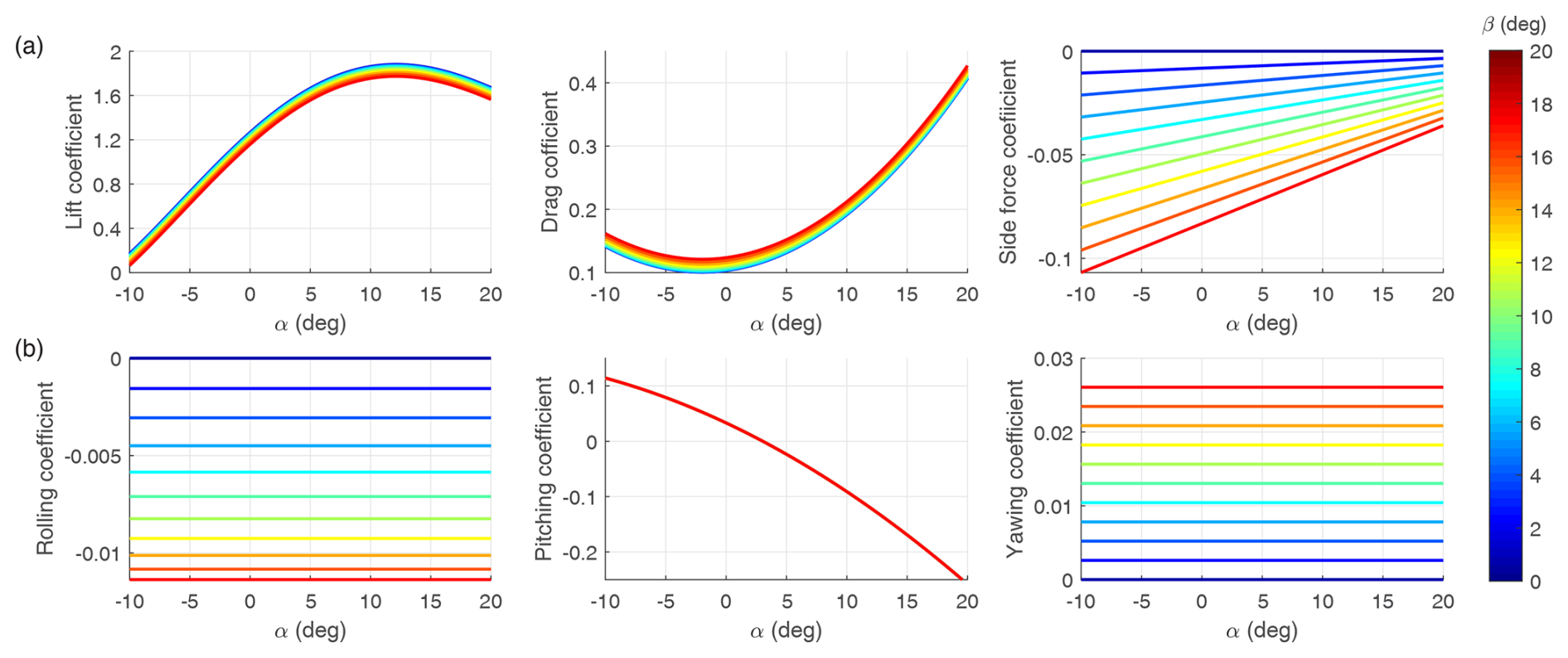
Figure 2 Static aerodynamic force (a) and moment (b) coefficients at full flaps and no control surface deflection.

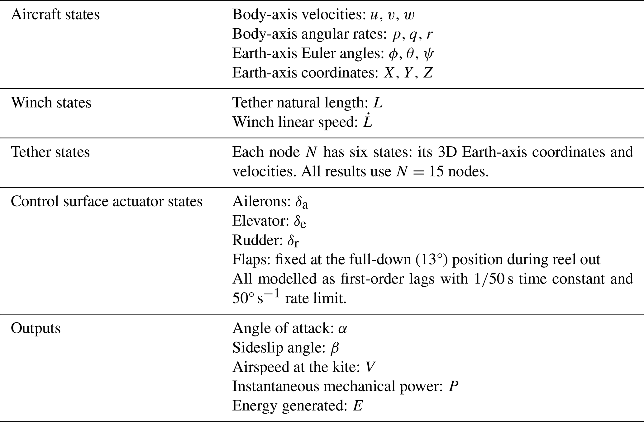
In its open loop configuration, the simulator has 108 states, comprising 12 states to describe the aircraft's motion in 3D space, 4 actuator states modelled as first-order lags with 50° s⁻¹ rate limit, 2 states to describe the ground winch, and 6N states to model the flexible tether, where N is the number of tether nodes between the winch and the kite. The N nodes discretised the tether into N+1 segments, which are connected by second-order mass-spring–damper elements. If the tether's natural length is fixed, the winch states can be discarded, and the model reduces to 102 states. A detailed description of the equations of motion can be found in Rapp et al. (2019). Table 1 summarises the open-loop states, control surface inputs, and outputs.

Table 1 Key elements of the open-loop model.

The tether's natural length L (excluding elastic extension) is regulated by an ideal ground winch, which is modelled as a cylinder of mass m_w = 25 kg and has a constant radius of R_w=0.25 m. The winch control system applies a winch force F_w that opposes the tether tension T at the winch. This gives a winch linear acceleration of

$$\begin{array}{}\text{(1)}& \ddot{L}=\left(T-F_{\mathrm{w}}\right){\displaystyle \frac{R_{\mathrm{w}}^{\mathrm{2}}}{I_{\mathrm{w}}}},\end{array}$$

where $I_{\mathrm{w}}=\mathrm{0.5}{m}_{\mathrm{w}}{R}_{\mathrm{w}}^{\mathrm{2}}$ is the winch moment of inertia. The winch speed (reel-out speed) $\dot{L}$ and natural length L are found by integrating Eq. (1) once and twice, respectively. Feedback control of the winch is provided by the term F_w, which is the output of a high-gain PID controller that tracks either a desired winch speed (keeping $\dot{L}$ close to constant) or a desired tether tension (keeping T close to constant). Apart from Fig. 30, all results in this paper with the winch active use the constant winch speed mode.

Provided that the winch is reeling out with positive tether tension, the instantaneous mechanical power P is calculated as

$$\begin{array}{}\text{(2)}& P=T\dot{L},\end{array}$$

and assuming no losses in the winch, Eq. (2) can be integrated to give the total energy generated up to time t

$$\begin{array}{}\text{(3)}& E={\int }_{t_{L=\mathrm{350}}}^{t}P\mathrm{d}t,\end{array}$$

where t_L=350 is the simulation time at the start of reel out, defined to be when the tether's natural length is 350 m. Reel out ends when L reaches 700 m.

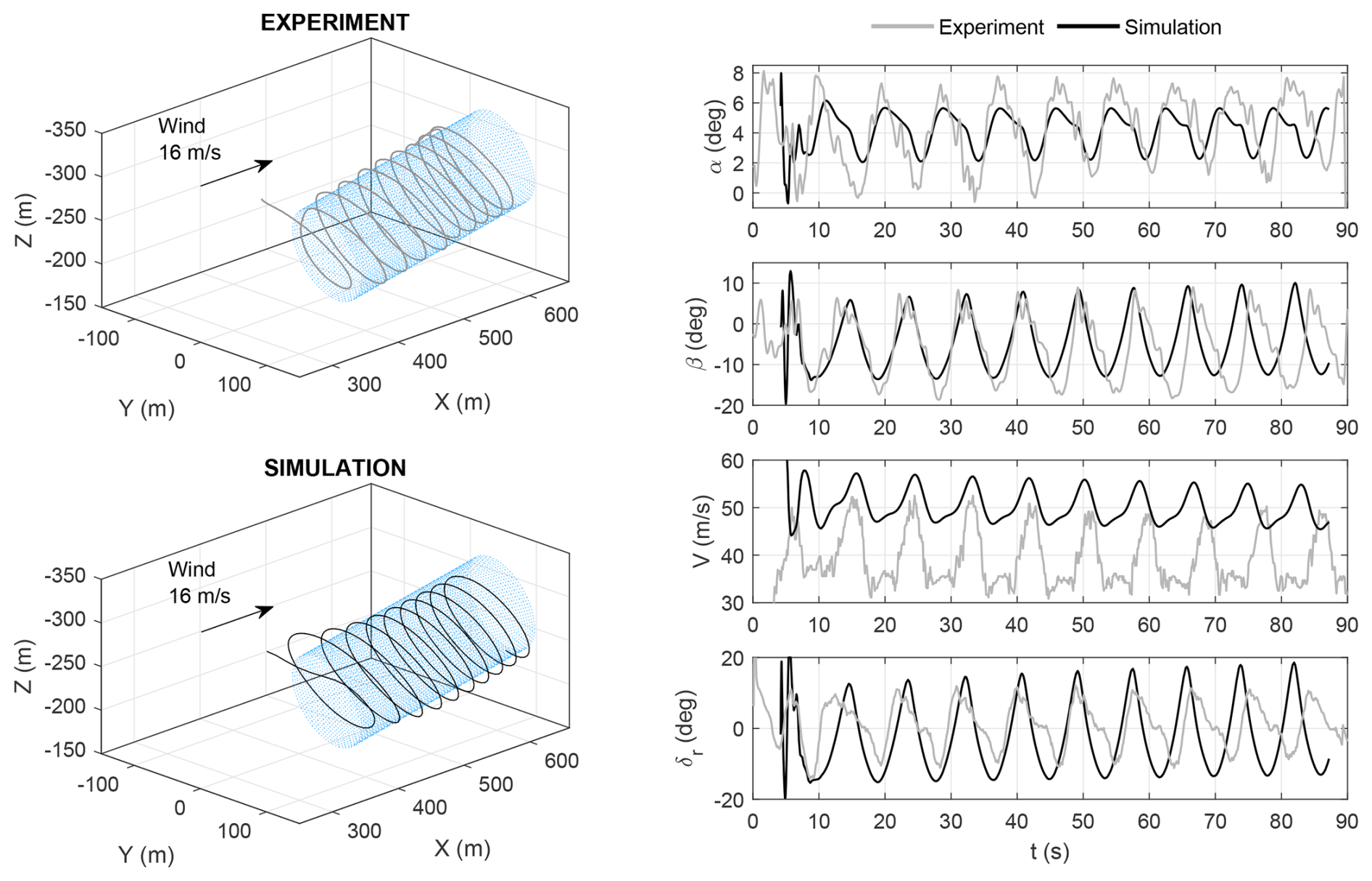
Figure 3 Experiment and simulated flight data (first presented in Nguyen et al., 2026a).

To verify the simulator's accuracy, we replicated a test flight in 16 m s⁻¹ wind. This test used an early flight control law presented in Mohammed et al. (2024a), which has only one proportional feedback loop on the rudder to generate yaw-induced roll. Elevator and aileron were fixed at −4 and 0°, respectively. Figure 3 shows that there is strong agreement between the recorded and simulated responses, apart from an offset in airspeed V due to a known sensor calibration fault that also affected angle of attack measurements. However, the shapes of the simulated and recorded airspeed are comparable, and other parameters show strong correlations. These results suggests that the simulator possesses sufficient accuracy for control law developments.

3 Baseline controller design

3.1 Key concept: tilting the reference plane

To implement the control law, three coordinate systems are required: Earth, reference, and production. The first two are needed for the current section and are now described. The Earth plane is defined by the three axes X, Y, and Z originating from the winch and pointing in the north, east, and down directions, respectively (see Fig. 4a). Three Euler angles describe the kite's body-axis orientation with respect to the Earth plane: ϕ (roll), θ (pitch), and ψ (yaw). Unless otherwise noted, the wind is assumed to be uniform and travels from south to north at a speed of 14 m s⁻¹.

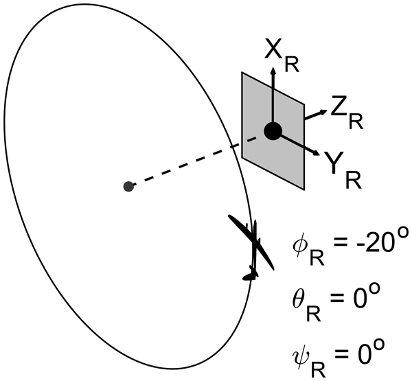
The reference plane is a “guidance plane” that provides a second set of Euler angles for the roll controller. Three axes X_R, Y_R, and Z_R define the reference plane. They also originate from the winch but have different orientations with respect to the Earth's axes. To construct the reference plane, start with its axes X_R, Y_R, and Z_R aligned with the Earth's axes X, Y, and Z, then apply the following right-hand rotations.

• Rotate Z_R by an angle ζ_R (zeta for aZimuth).

• Rotate Y_R axis by an angle λ_R+ 90° (lambda for eLevation).

• Rotate X_R by 180°.

These three rotations result in the reference plane having an orientation as shown in Fig. 4b – depicting λ_R and ζ_R having small positive values. Note that when ${\mathit{\lambda }}_{\mathrm{R}}={\mathit{\zeta }}_{\mathrm{R}}=\mathrm{0}$°, Z_R points in the negative X direction, and X_R points in the negative Z direction. From here, we obtain another set of Euler angles [ϕ_R, θ_R, ψ_R] that depicts the kite's roll, pitch, and yaw angles with respect to the reference plane. To aid understanding, Fig. 5 depicts a special case of ${\mathit{\lambda }}_{\mathrm{R}}={\mathit{\zeta }}_{\mathrm{R}}=\mathrm{0}$° with the kite in a south-bound, wing-level, climbing attitude. The corresponding Euler angles on the Earth and reference planes are shown. Subsequent analysis does not require the use of the kite's reference plane yaw angle ψ_R. To simplify illustrations, the reference plane will be depicted by a single dashed line originating from the winch and pointing in negative Z_R direction, as shown in Figs. 4b and 5b. Appendix A provides the mathematical operations for converting Euler angles from Earth to reference plane.

Figure 4 Two coordinate systems: Earth (a) and reference plane (b).

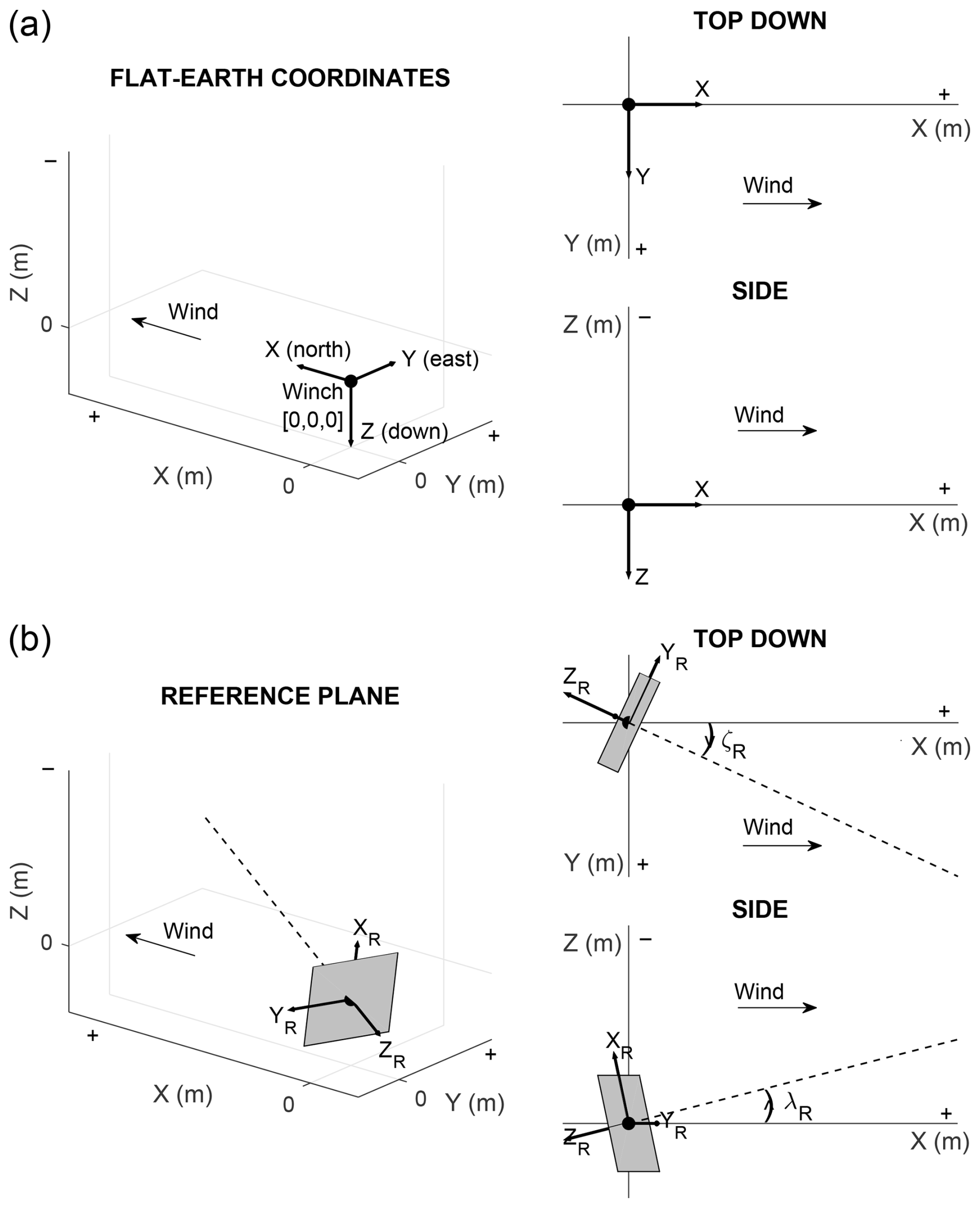
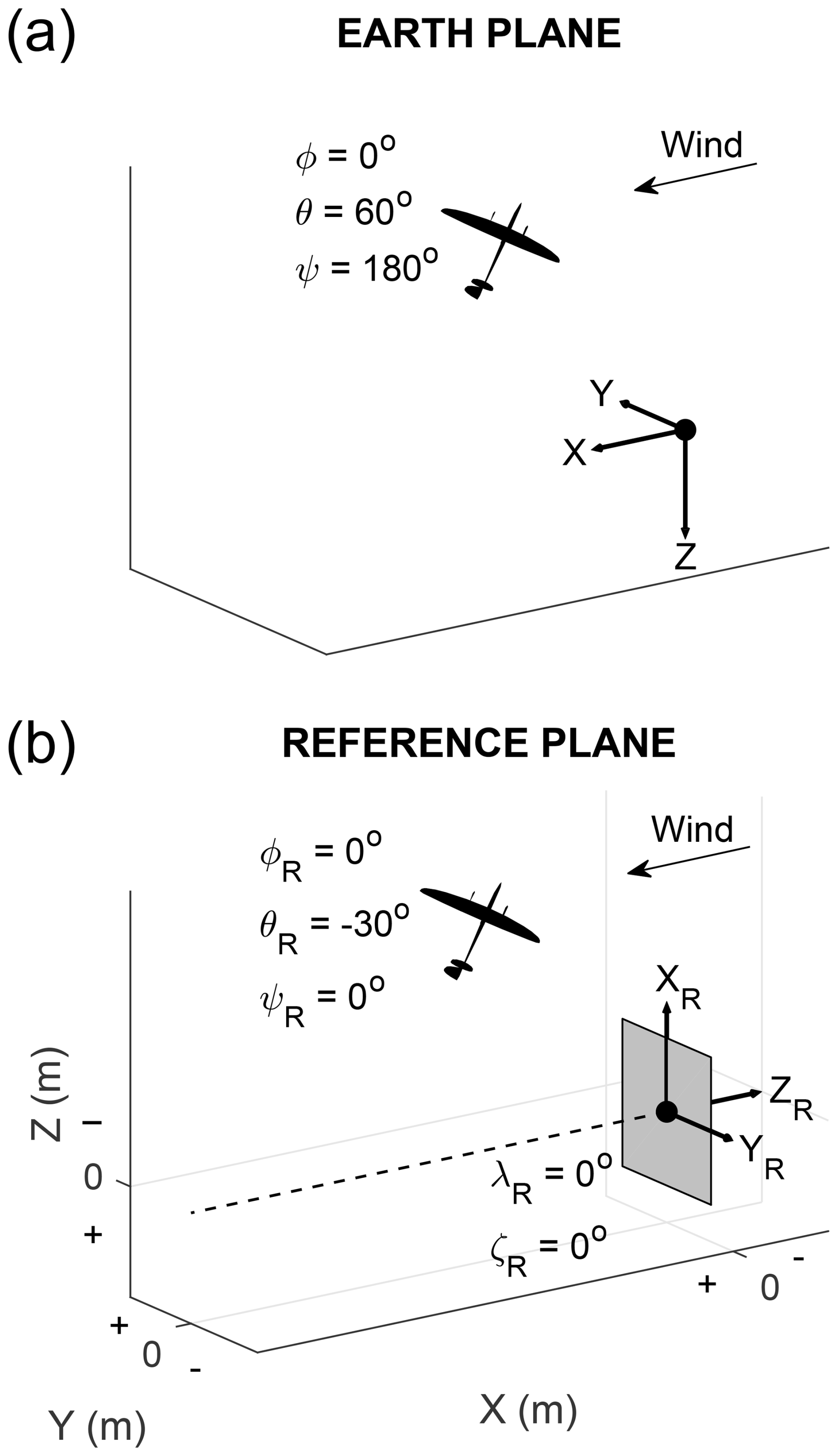
Figure 5 Illustrations of Euler angles on the Earth plane (a) and reference plane with ${\mathit{\lambda }}_{\mathrm{R}}={\mathit{\zeta }}_{\mathrm{R}}=\mathrm{0}$° (b).

We now discuss the flight controller. The principal idea is to use ailerons to track the roll angle ϕ_R on the reference plane, not ϕ on the Earth plane. Assuming that gravity and wind are not present, the kite has its own propulsion, and the tether length is fixed, then the trajectory will converge to a circular orbit on a plane parallel to the reference plane as shown in Fig. 6. This convergence is facilitated by two elements: the fixed-length tether preventing the kite from “climbing” away from the reference plane and converging to a helical trajectory and the roll controller keeping ϕ_R and hence radius constant. From this arrangement, we can shift the centre of the circle to a desired location by adjusting the reference plane orientation via λ_R and ζ_R. Equilibrium trim exists in this hypothetical scenario. However, AWES derive their propulsive force from the wind and operate in the presence of gravity, both of which act as external periodic disturbances that require a cyclic control input to compensate (Nguyen et al., 2026b). This cyclic input can be obtained by configuring the controller to track a fixed roll angle set point ${\mathit{\varphi }}_{{\mathrm{R}}_{\mathrm{SP}}}$ and accepting the subsequent oscillations caused by gravity and the wind.

Figure 6 Example left-roll circular orbit as defined by the reference plane.

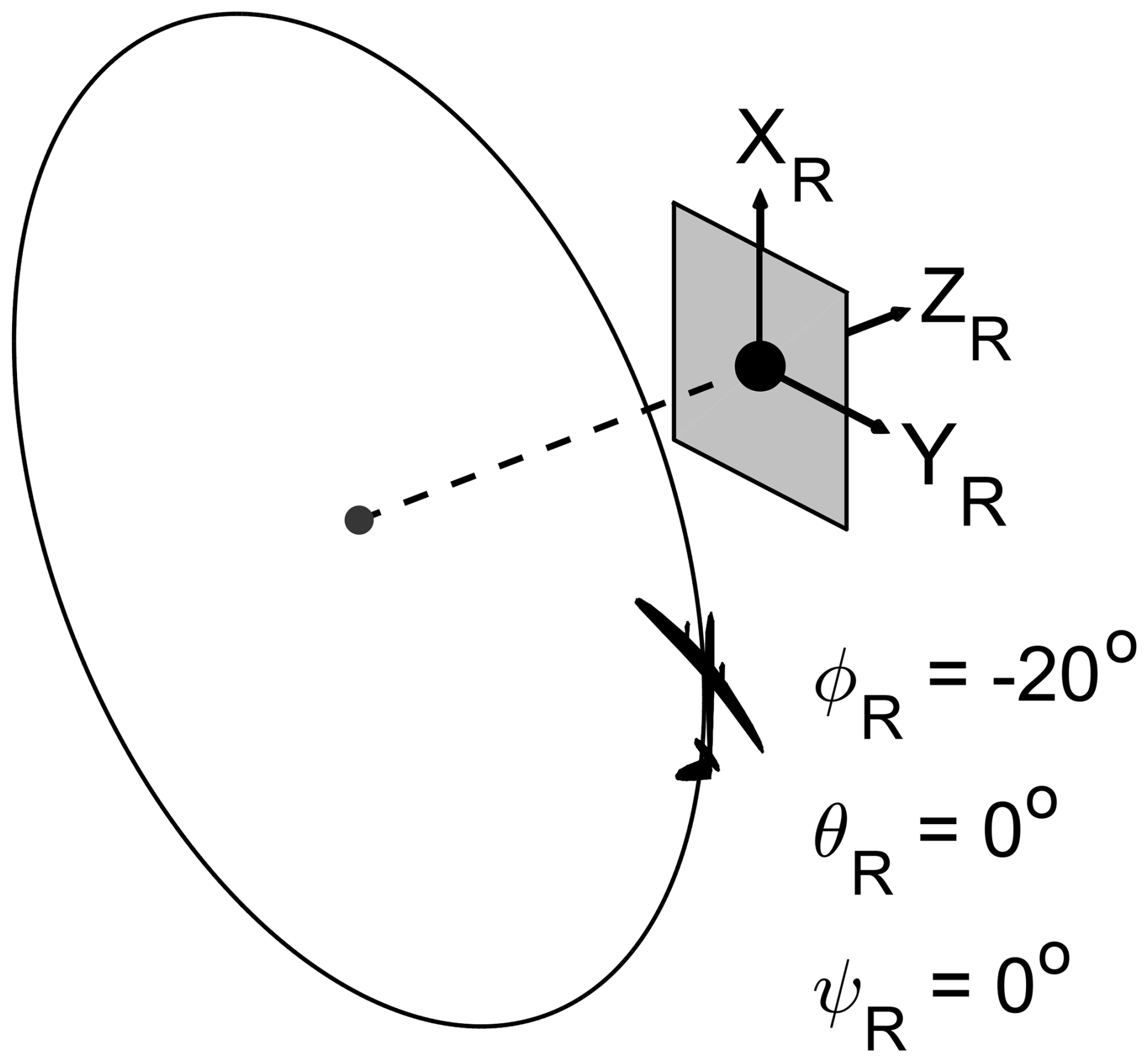
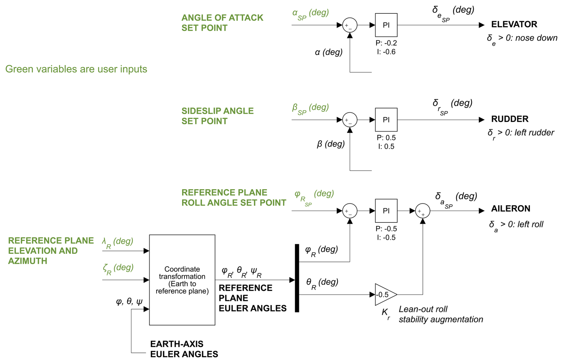
Figure 7 Basic flight control system (subsequently referred to as the inner loop). The Earth-to-reference-plane coordinate transformation is presented in Appendix A.

Figure 7 presents the proposed flight control system. For convenience, the following shorthand notation for proportional-integral control is used throughout the paper.

$$\begin{array}{}\text{(4)}& \mathrm{PI}\left(x_{\mathrm{SP}},x\right)=K_{\mathrm{P}}\left(x_{\mathrm{SP}}-x\right)+K_{\mathrm{I}}\int \left(x_{\mathrm{SP}}-x\right)\mathrm{d}t,\end{array}$$

where x_SP and x are the set point (SP) and feedback signal, and K_P and K_I are the proportional and integral gains. Three proportional-integral (PI) loops are used. The pitch and yaw channels channel adjust the elevator and rudder to track the desired angle of attack and sideslip set points. For the ailerons, their role is to track a demanded roll angle ${\mathit{\varphi }}_{{\mathrm{R}}_{\mathrm{SP}}}$ on the reference plane. This roll control method requires knowledge of the reference plane's orientation λ_R and ζ_R. In this section, we treat these two angles as user inputs, and Sect. 3.2 will explain how λ_R and ζ_R can be controlled automatically by the outer loop. Accordingly, the demanded control surface deflections are governed by the following feedback law.

$$\begin{array}{}\text{(5)}& {\displaystyle }{\mathit{\delta }}_{{\mathrm{e}}_{\mathrm{SP}}}=\mathrm{PI}({\mathit{\alpha }}_{\mathrm{SP}},\mathit{\alpha })\text{(6)}& {\displaystyle }{\mathit{\delta }}_{{\mathrm{r}}_{\mathrm{SP}}}=\mathrm{PI}({\mathit{\beta }}_{\mathrm{SP}},\mathit{\beta })\text{(7)}& {\displaystyle }{\mathit{\delta }}_{{\mathrm{a}}_{\mathrm{SP}}}=\mathrm{PI}\left({\mathit{\varphi }}_{{\mathrm{R}}_{\mathrm{SP}}},{\mathit{\varphi }}_{\mathrm{R}}\right)+K_{\mathrm{r}}{\mathit{\theta }}_{\mathrm{R}}\end{array}$$

The second term in Eq. (7) multiplies the reference-plane pitch angle by a proportional gain K_r. This pitch-roll cross-feeding signal counteracts the roll instability encountered in large-radius tethered circular flight, which was first reported in one of our earlier studies (see the discussion surrounding Eq. 1 in Nguyen et al., 2026a). The sign of K_r reflects flight direction. For trajectories where the circle's centre is on the port (left) wing's side, K_r should be negative. By conventional flight control standards, the PI-only feedback scheme in Fig. 7 can be stable but may not provide adequate handling qualities – mainly due to the clear separation between fast and slow dynamics in the pitch and yaw responses. Higher performance is usually achieved by adding an inner stability augmentation loop that feeds back both fast (body-axis angular rates) and slow (body-axis angles) variables. Those performance-enhancement elements are deliberately left out in this work to demonstrate the robustness of our flight control scheme, which can handle sub-optimal handling qualities caused by rudimentary inner-loop designs.

We now examine a closed-loop response with the tether length fixed (i.e. $\dot{L}=\ddot{L}=\mathrm{0}$) at 350 m – a typical length at the start of reel out for the KM1 AWES. The reference plane orientation is [λ_R, ${\mathit{\zeta }}_{\mathrm{R}}]=[\mathrm{0}\mathit{°},\mathrm{0}\mathit{°}]$, and a representative combination of set points [α_SP, β_SP, ${\mathit{\varphi }}_{{\mathrm{R}}_{\mathrm{SP}}}]=[\mathrm{6}\mathit{°},\mathrm{0}\mathit{°},-\mathrm{15}\mathit{°}]$ is chosen. Negative ${\mathit{\varphi }}_{{\mathrm{R}}_{\mathrm{SP}}}$ indicates the circle centre is on the port side of the wing, which is assumed throughout this paper without loss of generality. In this arrangement, the kite follows a circular orbit as shown in Fig. 8a. Inspecting the time history of this trajectory (Fig. 8b) reveals that the controller has entered a small limit cycle with periodic forcing inputs. This behaviour is expected, as our previous work in Nguyen et al. (2026b) has shown that tracking a set of specified α, β, and ϕ_R using fixed control surfaces (i.e. an equilibrium response) is only possible when gravity is ignored. The resulting gravity-free orbit is normal to the wind and has its circle centre on the ground, which overlaps the winch when viewed from the wind-facing direction. When gravity is included as shown in Fig. 8a, we see the circle centre shifting downward due to weight and slightly sideways due to lift asymmetry (from the wind-facing view: the kite climbs at the 3 o'clock position and descends at the 9 o'clock point, so the latter generates more lift, pushing the orbit centre to the side). Gravity also changes direction periodically with respect to the kite's body axis throughout the cycle. All of the above factors mean that the desired closed-loop trajectory is a limit cycle, so control surface movements should be cyclic to counteract the external periodic disturbance. Nevertheless, all three controlled variables α, β, and ϕ_R oscillate with small amplitudes around the desired values, and the cyclic control surface movements are also small.

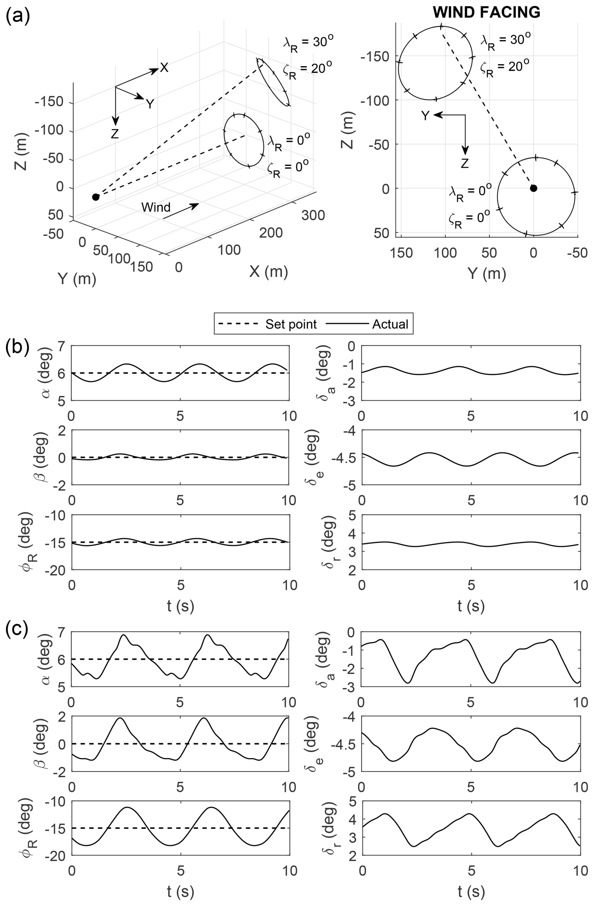
Figure 8 Closed-loop trajectories (a) and time histories (b and c) with two different reference plane orientations. The time histories of [λ_R, ζ_R] = [0°, 0°] and [λ_R, ${\mathit{\zeta }}_{\mathrm{R}}]=[\mathrm{30}\mathit{°},\mathrm{20}\mathit{°}]$ are shown in (b) and (c), respectively.

The reference plane orientation is now changed to non-trivial values of [λ_R, ${\mathit{\zeta }}_{\mathrm{R}}]=[\mathrm{30}\mathit{°},\mathrm{20}\mathit{°}]$. Figure 8a shows the resulting closed-loop response. The kite still follows a circular path, which is now at a slight angle to the wind due to the new reference plane's orientation. Larger magnitudes in λ_R and ζ_R result in more longitudinal and lateral shifting, which become less effective as the circular orbit moves further away from its ideal location of being normal to the wind (achieved only when gravity is ignored and [λ_R, ${\mathit{\zeta }}_{\mathrm{R}}]=[\mathrm{0}\mathit{°},\mathrm{0}\mathit{°}]$). A consequence of shifting further away from the ideal location is higher limit cycle amplitudes, as seen in Fig. 8c vs Fig. 8b. This behaviour is congruent with our previous observations, which noted that circular flight further away from the ideal location requires larger cyclic control inputs (Nguyen et al., 2026b). Nevertheless, as long as there is enough control power and sufficient wind to prevent airspeed from dropping to the stall point, the current flight control scheme will keep the kite in a stable circular orbit.

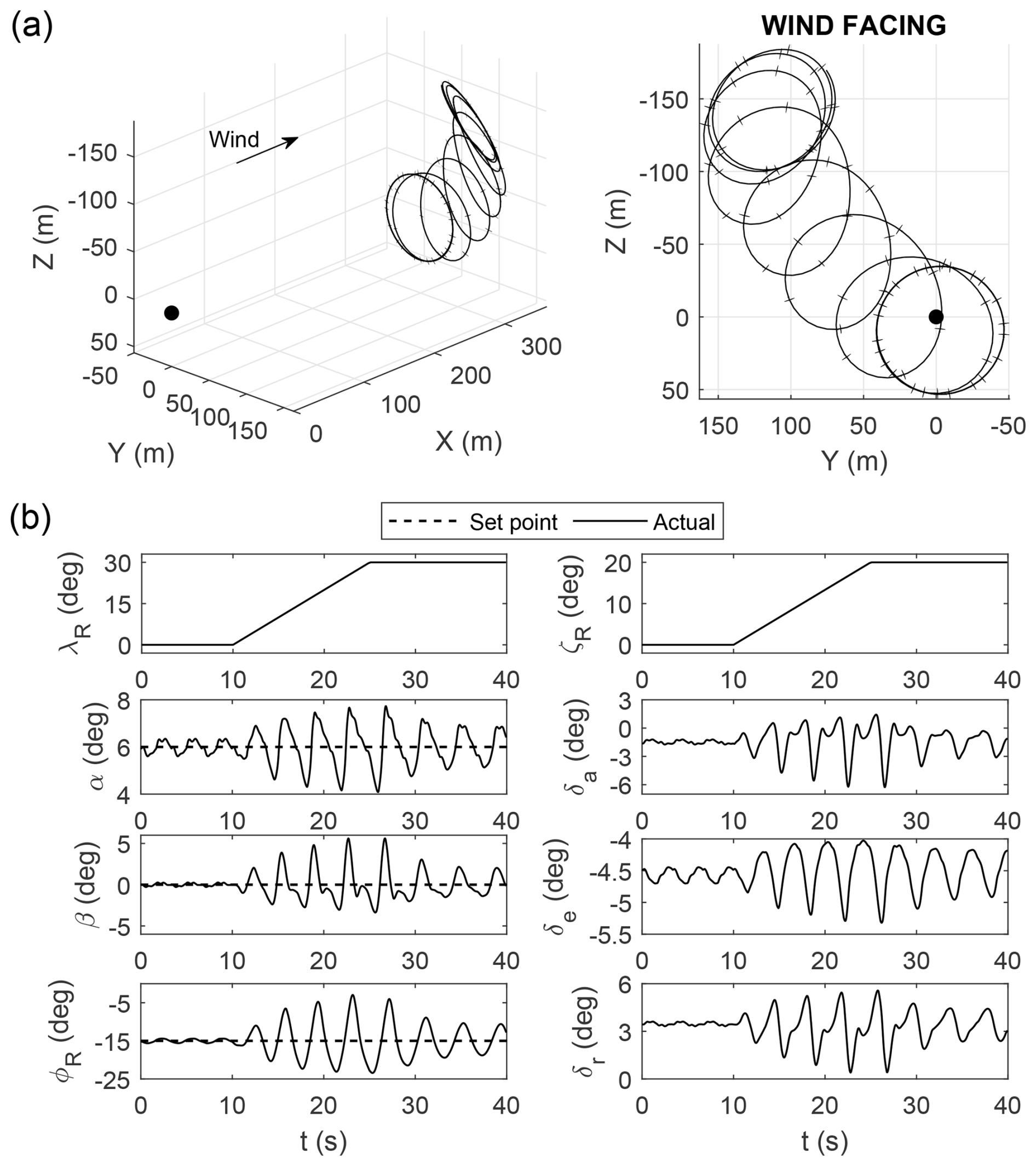
Results in Fig. 8 suggests that the orbit centre can be dynamically shifted by adjusting the reference plane's orientation. To demonstrate this point, Fig. 9 shows the kite's response to two simultaneous ramp inputs in λ_R and ζ_R. Both ramps last 15 s, starting from [λ_R, ζ_R] = [0°, 0°] and ending at [λ_R, ζ_R] = [30°, 20°]. The resulting trajectory shows that the kite achieves a gradual transition between the two conditions while maintaining circular flight throughout the manoeuvre. This method of transitioning between different operating points is more desirable than taking a straight-line path to the destination, which risks running out of airspeed mid-flight due to the lack of a dedicated propulsion unit. The fact that the kite maintains circular flight by itself also simplifies control design significantly, as there is no need to design the exact path in 3D space for the kite to follow. In other words, the path-planning problem is reduced to adjusting two variables λ_R and ζ_R by the right rate and magnitude.

Figure 9 Response to simultaneous ramp inputs in λ_R and ζ_R.

Lastly, to adjust the circle radius, one simply needs to change the set point for the reference plane roll angle ${\mathit{\varphi }}_{R_{\mathrm{SP}}}$. Our previous work has shown that leaning more into the turn reduces the radius, while leaning out widens the orbit (Nguyen et al., 2026b). In this example of a left-turning trajectory, increasing the radius requires a more positive ϕ_R. Figure 10 shows two circular trajectories corresponding to ${\mathit{\varphi }}_{R_{\mathrm{SP}}}=-\mathrm{15}$ and 0°. It can be seen that the 0° case achieves a larger radius as intended.

This section has shown that by using the ailerons to track a fixed roll angle on a user-defined reference plane, the kite can keep itself in circular orbit without requiring complex path planning. Tilting the reference plane (i.e. adjusting λ_R and ζ_R) provides a means to shift the circular orbit to a desired location. Additionally, the radius can be widened or tightened by changing the set point for the reference plane roll angle. These ideas provide the foundation for a circular reel-out controller, which is described in the following section.

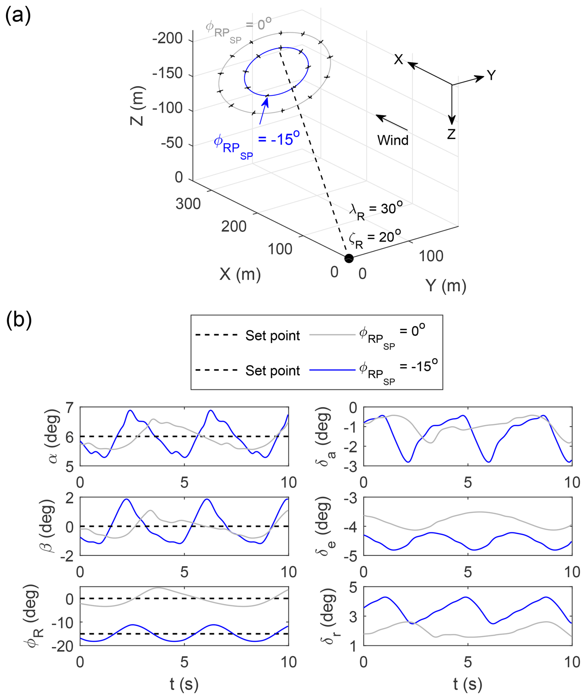
Figure 10 Closed-loop trajectories (a) and time histories (b) with different ${\mathit{\varphi }}_{{\mathrm{R}}_{\mathrm{SP}}}$. The kite is drawn true to scale at 0.5 s intervals.

3.2 Outer loop: tracking a target cylinder

During circular reel out, the kite flies in a helical trajectory resembling a spring that “wraps” around an imaginary cylinder, shown in light blue in Fig. 11. The cylinder can be defined by a third coordinate system called the production plane. Its orientation with respect to the Earth's plane is defined by three axes X_P, Y_P, and Z_P, along with two angles λ_P and ζ_P – constructed in a similar manner to λ_R and ζ_R in the reference plane. However, unlike the reference plane, the production plane does not have to originate from the winch. The user can specify the location of the production plane's origin, which is shown as point P in the top plot of Fig. 11. The Earth-axis coordinate of point P is referred to as P_X, P_Y, and P_Z. From here, the target cylinder is defined to have a circular base on the X_P-Y_P plane, centred around point P with radius R_SP, and extends in the negative Z_P direction. For convenience, we refer to the kite's location on the production plane as X_P, Y_P, and Z_P. For instance, Fig. 11 depicts the production plane originating from point P with Earth-axis coordinates [P_X, P_Y, $P_Z]=[\mathrm{200},\mathrm{0},-\mathrm{150}]$ m. If the kite is also located at point P, then the kite's location is [X, Y, Z] = [200, 0, −150] m using Earth-axis coordinates, and [X_P, Y_P, $Z_{\mathrm{P}}]=[\mathrm{0},\mathrm{0},\mathrm{0}]$ m on the production plane. The equations to convert from Earth to production plane coordinates are provided in Appendix B.

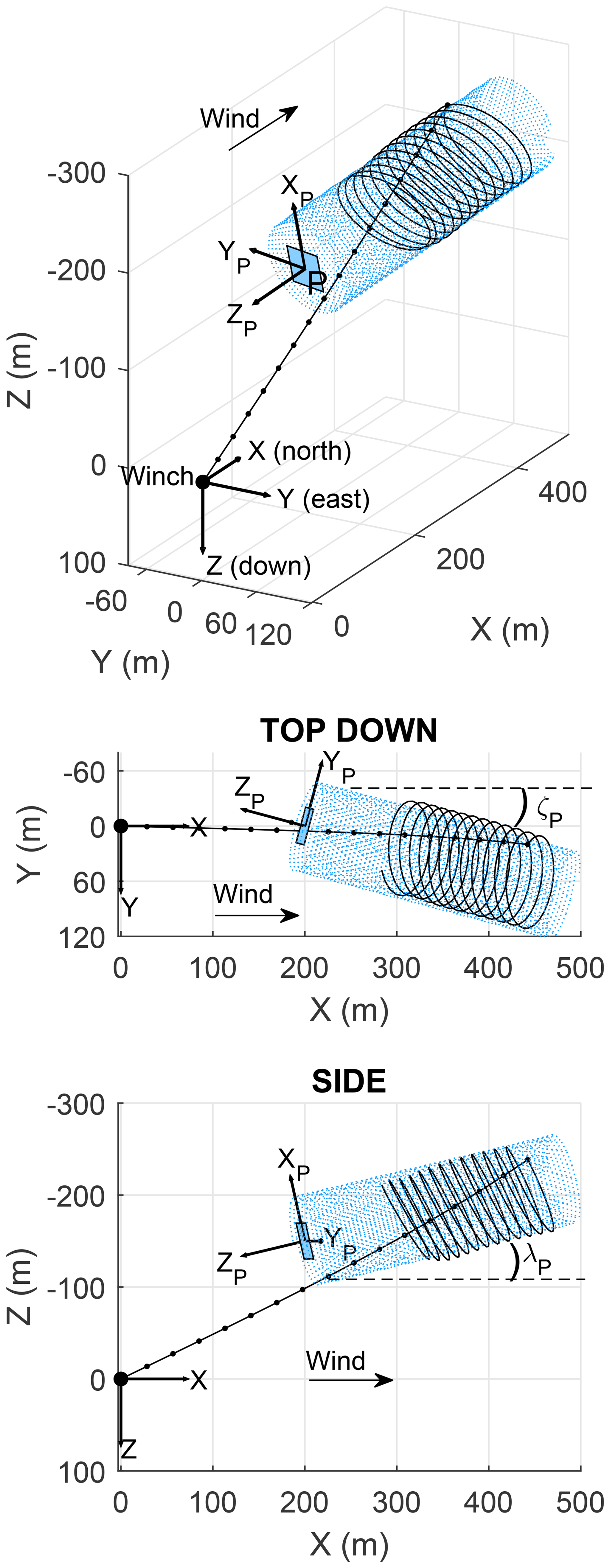
Figure 11 Target cylinder (light blue) and the production plane (blue square with axes X_P, Y_P, and Z_P).

The kite's radius on the production plane is calculated as $R=\sqrt{X_{\mathrm{P}}^{\mathrm{2}}+Y_{\mathrm{P}}^{\mathrm{2}}}$. To keep R close to the desired radius R_SP, the three inputs to the inner loop ${\mathit{\varphi }}_{{\mathrm{R}}_{\mathrm{SP}}}$, λ_R, and ζ_R need to be adjusted automatically via a feedback scheme. We refer to this second feedback layer as the outer loop, which works based on the following principles.

• Adjust the amount of roll via ${\mathit{\varphi }}_{{\mathrm{R}}_{\mathrm{SP}}}$ to keep the actual radius R close to the desired radius R_SP.

• Move the circle's centre up or down by adjusting λ_R, so that the kite's production-plane coordinate X_P is kept oscillating around zero.

• Move the circle's centre left or right by adjusting ζ_R, so that the kite's production-plane coordinate Y_P is kept oscillating around zero.

This feedback scheme can be achieved using three additional PI controllers as shown in Fig. 12. The components previously presented in Fig. 7 form the inner loop, while three new PI elements form the outer loop. In addition, a low-pass filter with time constant τ=10 s is used on the R feedback path to reduce ${\mathit{\varphi }}_{{\mathrm{R}}_{\mathrm{SP}}}$ oscillation since large changes in radius can be achieved by a gradual adjustment in ${\mathit{\varphi }}_{{\mathrm{R}}_{\mathrm{SP}}}$. The resulting outer loop dynamics is described by Eqs. (8)–(11).

$$\begin{array}{}\text{(8)}& {\displaystyle }{\dot{R}}_{\mathrm{filtered}}=-{\displaystyle \frac{\mathrm{1}}{\mathit{\tau }}}{R}_{\mathrm{filtered}}+{\displaystyle \frac{\mathrm{1}}{\mathit{\tau }}}R\text{(9)}& {\displaystyle }{\mathit{\varphi }}_{{\mathrm{R}}_{\mathrm{SP}}}=\mathrm{PI}(R_{\mathrm{SP}},R_{\mathrm{filtered}})\text{(10)}& {\displaystyle }{\mathit{\lambda }}_{\mathrm{R}}=\mathrm{PI}(\mathrm{0},X_{\mathrm{P}})\text{(11)}& {\displaystyle }{\mathit{\zeta }}_{\mathrm{R}}=\mathrm{PI}\left(\mathrm{0},Y_{\mathrm{P}}\right)\end{array}$$

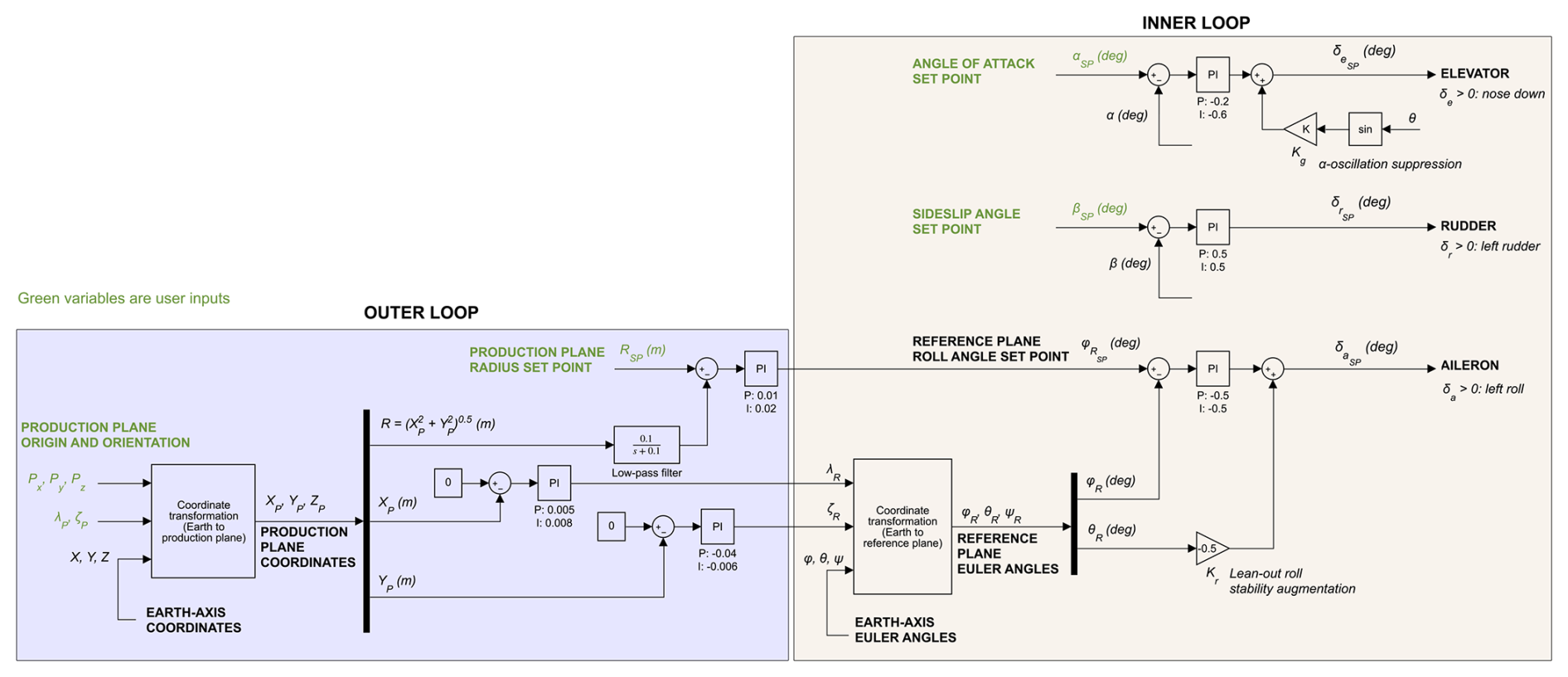
Figure 12 Full flight control system. The Earth-to-production-plane coordinate transformation is presented in Appendix B.

In addition, the inner loop in Fig. 12 shows an optional K_gsin θ feedback path to the elevator. This term reduces the angle of attack oscillation amplitude and is only used in Sect. 6. All results in Sects. 4–5 do not use this additional term, effectively having K_g=0. The other control gains are kept identical throughout the paper for circular flights.

An example reel-out trajectory with the tether visible is depicted in Fig. 11. This helical flight path wraps around the cylinder without requiring an exact 3D space to be specified. Therefore, the flight control problem has been reduced to a one-degree-of-freedom task handled by the ailerons (as elevator and rudder are only used for adjusting angle of attack and sideslip to achieve aerodynamic efficiency). The Julia code for the full flight control system is provided in a public depository (Nguyen, 2026). This code and the main body of this paper have been written to provide enough context for automatic implementation by a large language model. For instance, the authors have successfully used Claude Code by Anthropic (version 2.1, run as an extension in Visual Studio Code) to build a fully functional closed-loop system in MATLAB. Claude Code was granted access to only this article and an open-loop version of the simulator.

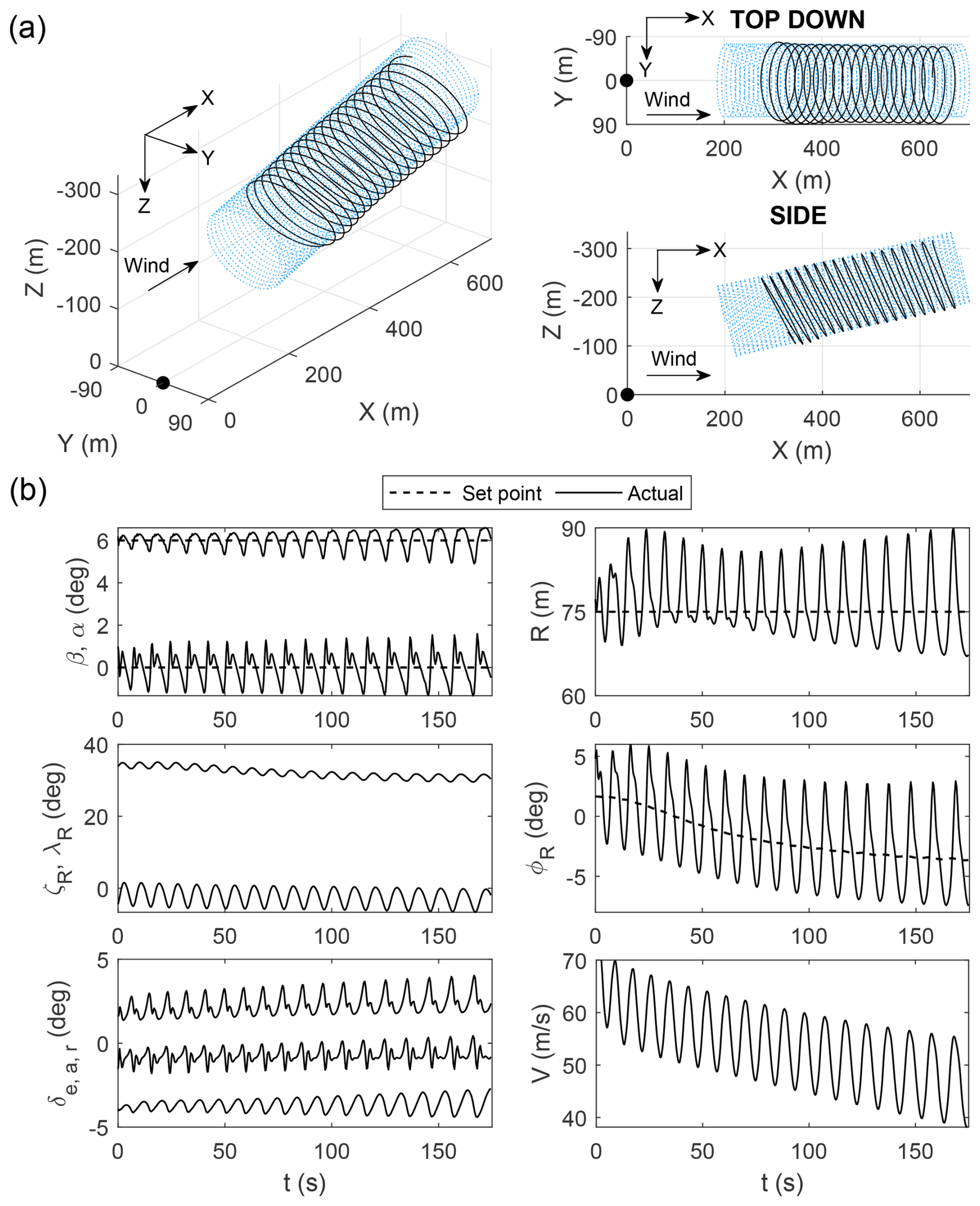
Figure 13 A typical circular reel-out trajectory with parameters $\mathbf{P}=[\mathrm{200},\mathrm{0},-\mathrm{150}]$ m, [λ_P, ${\mathit{\zeta }}_{\mathrm{P}}]=[\mathrm{13}\mathit{°},\mathrm{0}\mathit{°}]$, and R_SP=75 m. The winch speed is kept constant at 2.0 m s⁻¹.

4 Results

4.1 Uniform wind

A typical reel-out trajectory is presented in Fig. 13, which tracks a target cylinder of 50–75 m radius (75 m in this case), originating from point P with Earth-axis coordinate [P_X, P_Y, $P_Z]=[\mathrm{200},\mathrm{0},-\mathrm{150}]$ m, tilted up by 13°, and pointing in the downwind direction ([λ_P, ${\mathit{\zeta }}_{\mathrm{P}}]=[\mathrm{13}\mathit{°},\mathrm{0}\mathit{°}]$). Setting λ_P to 13° results in a slight climbing trajectory that reduces the risk of the tether scraping the ground at long tether length but at the cost of higher cosine losses (Diehl, 2013). In practice, this loss can be mitigated by stronger winds experienced at higher altitudes. Results in Fig. 13 shows the kite successfully achieving reference tracking in angle of attack, sideslip, and cylinder wrap-around. Note the second row in Fig. 13b, which shows the three output variables λ_R, ζ_R, and ${\mathit{\varphi }}_{{\mathrm{R}}_{\mathrm{SP}}}$ of the outer loop. All three variables require gradual adjustment as the tether length extends to compensate for increasing tether drag. By conventional feedback control standard, the variation in radius can be considered large, reaching 15 % above the set point toward the end of reel out. Nevertheless, the 3D trajectory suggests that this variation still results in a reasonable trajectory. Control surface usage increases as the tether length increases due to higher tether mass and drag, resulting in lower airspeed and hence reduced control effectiveness. Therefore, a limiting factor in how far the kite can reel out is control surface magnitude saturation (in addition to other efficiency issues that can be studied with an optimisation algorithm).

To further stress-test the controller, tracking performance with less ideal reel-out paths is now examined. Figure 14 shows a diagonal reel out, which is achieved by setting ζ_P to 15°. Sideway reel out is shown in Fig. 15, where both ζ_P and λ_P are 0°, but the target cylinder is shifted to the side by 100 m. Both instances show the kite successfully tracking the blue cylinder despite higher lateral force from the tether.

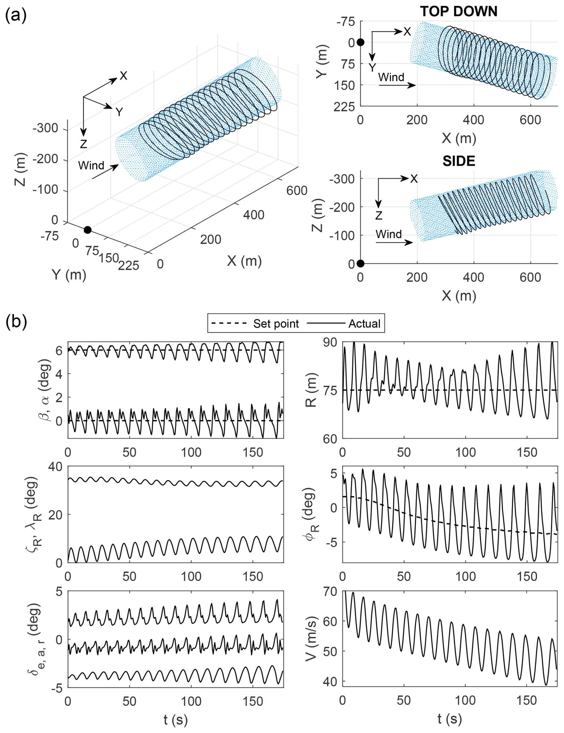
Figure 14 Diagonal reel out with parameters $\mathbf{P}=[\mathrm{200},\mathrm{0},-\mathrm{150}]$ m, [λ_P, ${\mathit{\zeta }}_{\mathrm{P}}]=[\mathrm{13}\mathit{°},\mathrm{15}\mathit{°}]$, and R_SP=75 m. The winch speed is kept constant at 2.0 m s⁻¹.

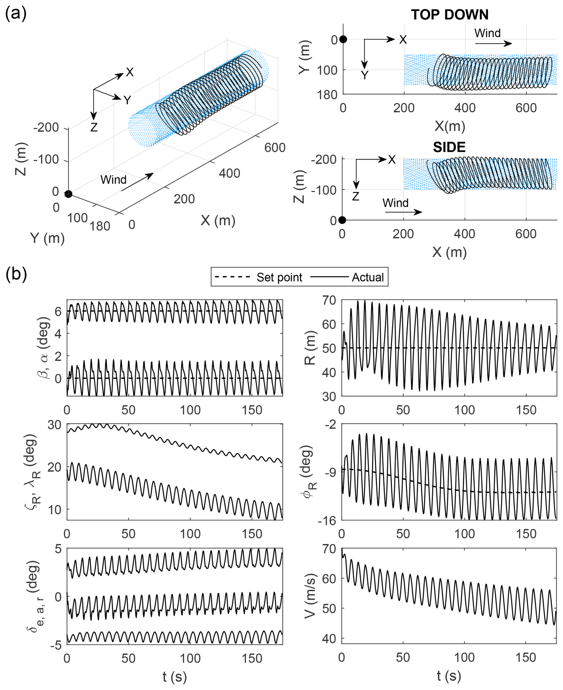
Figure 15 Sideway reel out with parameters $\mathbf{P}=[\mathrm{200},\mathrm{100},-\mathrm{150}]$ m, [λ_P, ${\mathit{\zeta }}_{\mathrm{P}}]=[\mathrm{0}\mathit{°},\mathrm{0}\mathit{°}]$, and R_SP=50 m. The winch speed is kept constant at 2.0 m s⁻¹.

For the final robustness tests, the target cylinder in Fig. 13 is flown again with the controller implemented in discrete form using a low sample rate of 20 Hz while subjected to a 0.1 s delay to all feedback variables. After 50 s of reeling out, the wind direction suddenly changes from 0 to 30°. Figures 16 and 17 show the closed-loop responses with and without corrective actions to the target cylinder to accommodate the new wind direction. In both cases, the kite successfully follows the target cylinder while tracking the angle of attack and sideslip set points despite the sub-optimal condition. Actuator rate limiting is not an issue, as a peak rate of only 14° s⁻¹ was recorded in the yaw channel of both figures. A lot of the oscillations before the wind-direction change can be attributed to the simple design of the inner loops, which exacerbates the poor transient responses in the presence of feedback delay and low sample time. As discussed in Sect. 3.1, better performance can be achieved with a more sophisticated inner loop. The outer loop, on the other hand, has demonstrated sufficient robustness to guide the kite in sub-optimal conditions even with a simple inner loop design.

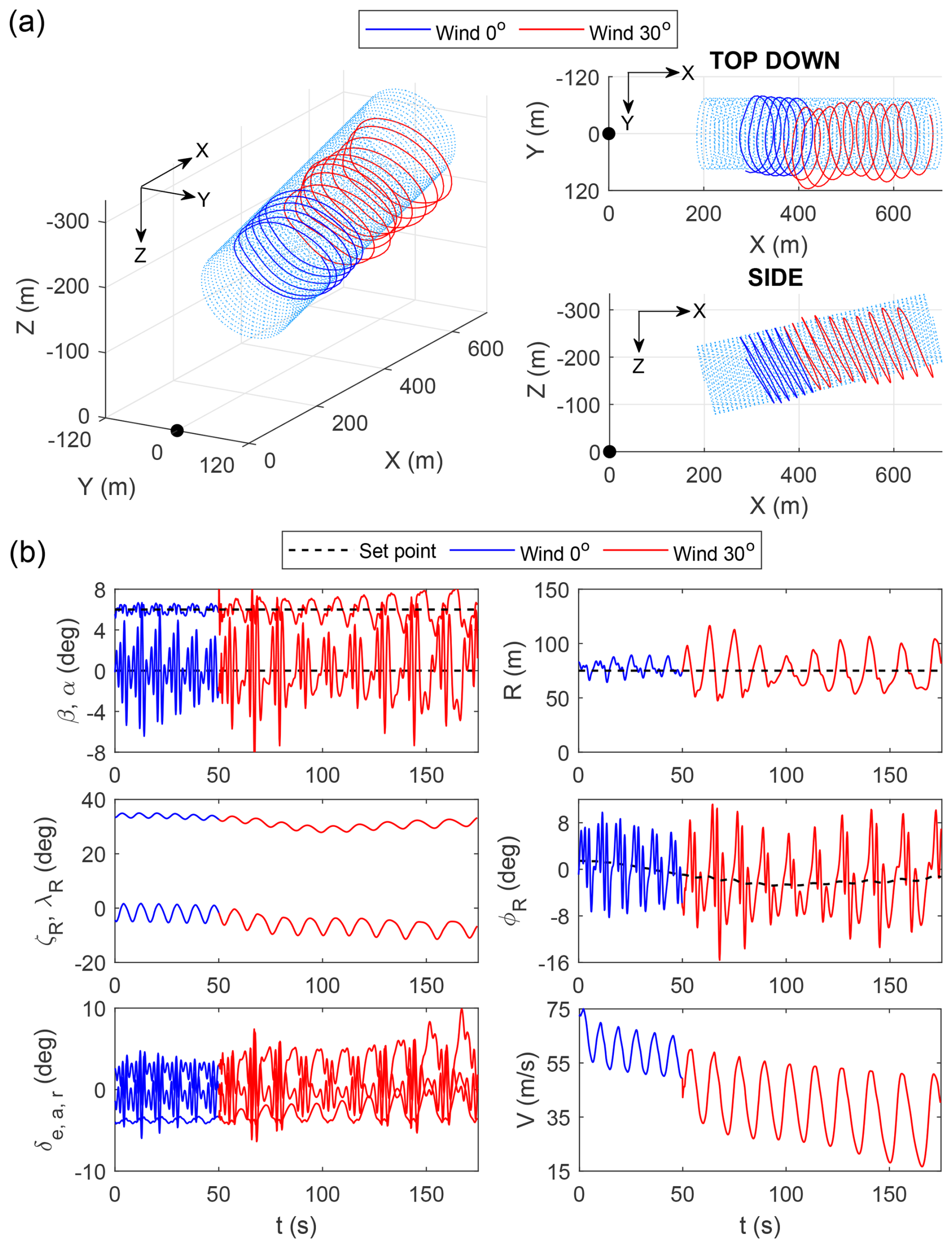
Figure 16 Closed-loop response to a sudden change in wind direction using a discrete controller (10 Hz) with feedback delay (0.1 s) and no corrective action to the target cylinder.

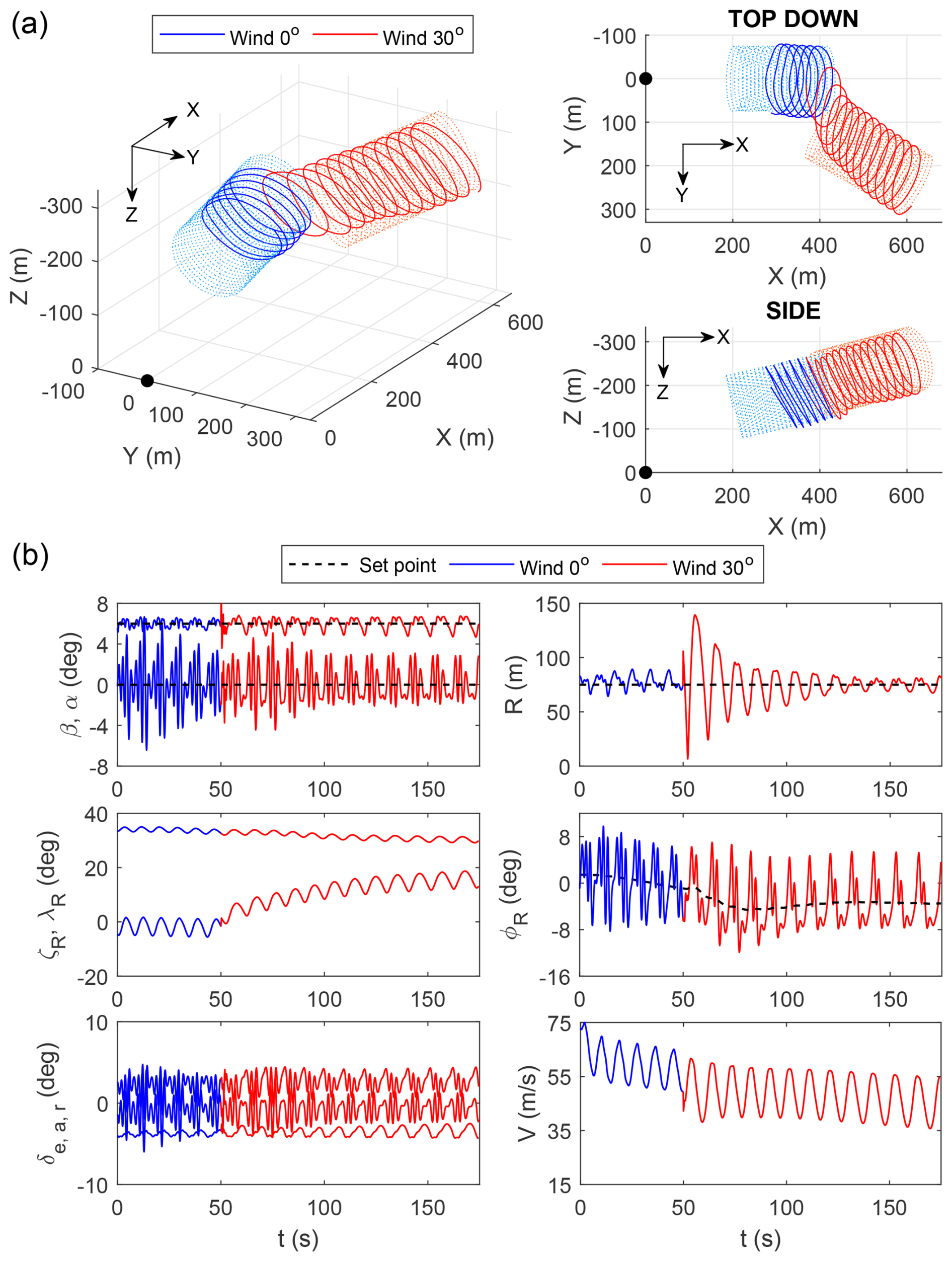
Figure 17 Closed-loop response to a sudden change in wind direction using the same discrete controller but with corrective actions to the target cylinder.

4.2 Non-uniform wind with turbulence

Experiments have shown that there is considerable variation in wind speed with height, so a feasible controller must be able to perform in a non-uniform wind field. The simulation is now augmented with realistic wind and turbulence conditions. Two wind fields shown in Fig. 18 are used. The first one (referred to as medium wind) has an average speed of 12.1 m s⁻¹ at 150 m height, and the second one (high wind) averages at 22.9 m s⁻¹ at 100 m. Both wind fields were derived from lidar data at Kitemill's test site in Lista, Norway, on two different days. Variations in the wind profile over time are also captured in the lidar data as shown in Fig. 18 and implemented in the simulation.

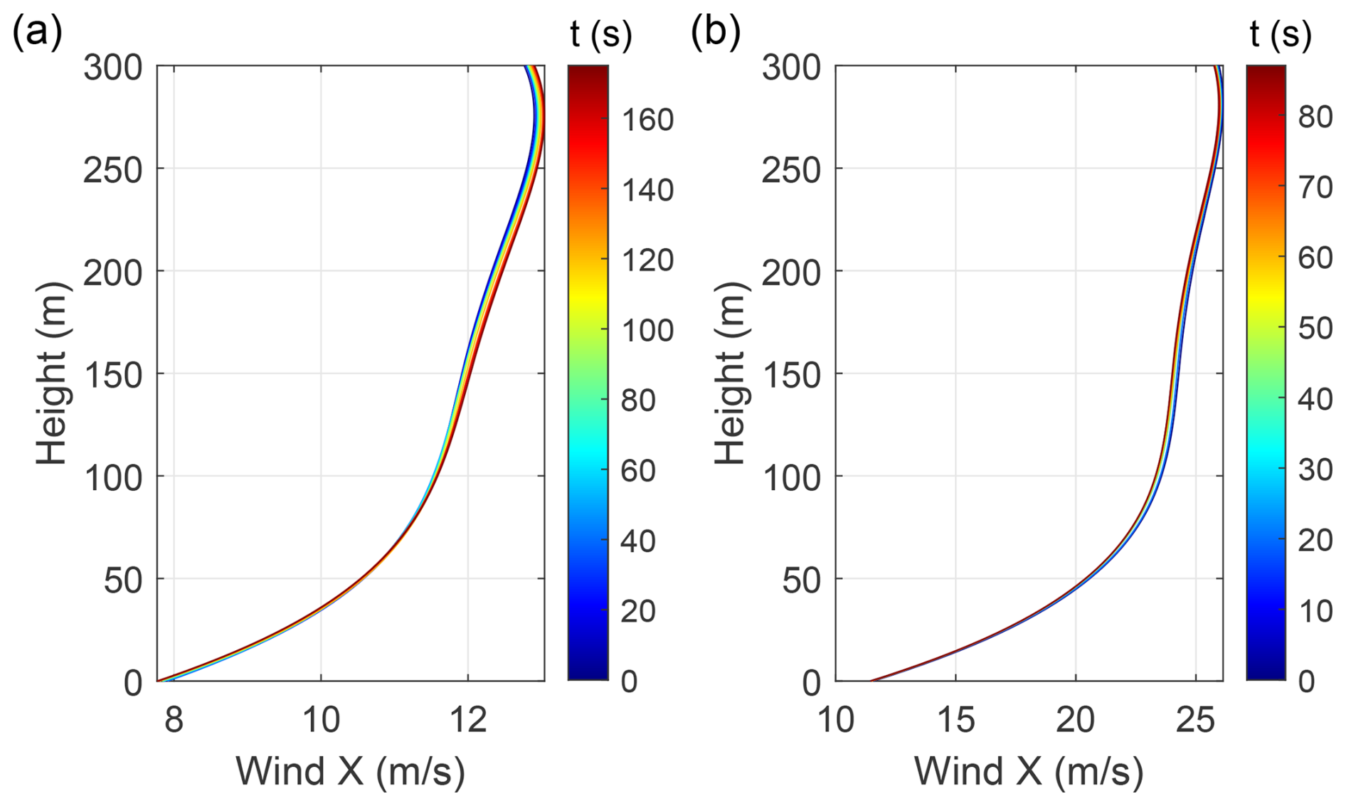
Figure 18 Medium (a) and high (b) wind fields implemented in the simulation based on lidar data.

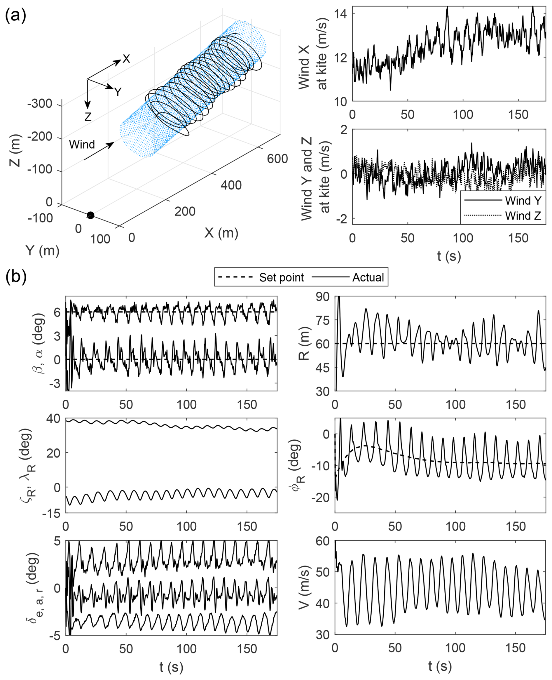
Figure 19 Reel out in medium wind and medium turbulence. The winch speed is kept constant at 2.0 m s⁻¹. A better tracking performance can be achieved by reducing the winch speed.

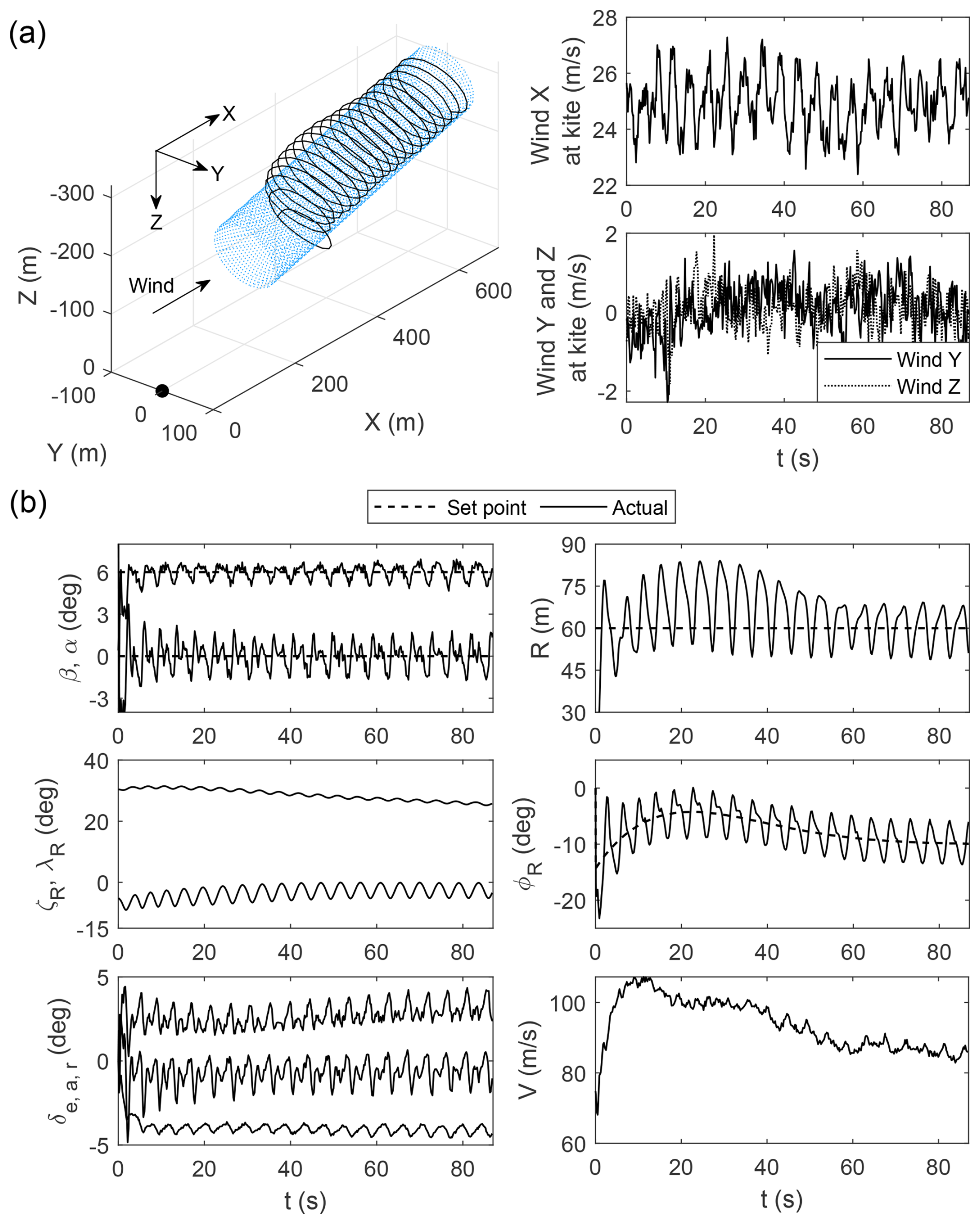
Figure 20 Reel out in high wind and high turbulence. The winch speed is kept constant at 4.0 m s⁻¹.

Additionally, lidar measurements at the site have shown that atmospheric turbulence is present, resulting in significant disturbances in both wind speed and direction. To capture this phenomenon, we implemented a turbulence box based on the Mann model (Mann, 1994). This box covers the 3D space flown by the kite with local wind velocity fluctuations due to atmospheric turbulence. Such fluctuations are added to the wind velocity seen by the kite as the turbulence box is convected downstream with the mean wind speed. This modelling approach follows Taylor's frozen turbulence hypothesis, which states that the turbulent eddies move downstream with the mean wind speed and assumes the structures remain mostly unchanged as they propagate (Taylor, 1937). Generating the turbulence box requires the Mann model parameters: dominant turbulence length scale L_M, amplitude parameter $\mathit{\alpha }{\mathit{\epsilon }}^{\mathrm{2}/\mathrm{3}}$ and anisotropy parameter Γ. The turbulence length scale and amplitude parameter have been estimated from flow field parameters (Kelly, 2018) measured by the lidar at the test site. Two different turbulence cases have been employed in the simulations according to the turbulence measured at the site, referred to as medium turbulence ($\mathit{\alpha }{\mathit{\epsilon }}^{\mathrm{2}/\mathrm{3}}=\mathrm{0.0108}$) and high turbulence ($\mathit{\alpha }{\mathit{\epsilon }}^{\mathrm{2}/\mathrm{3}}=\mathrm{0.0267}$). The turbulence length scale has been defined as L_M=78.44 m for both cases, being representative of the site, while the anisotropy parameter has been assumed as Γ=3.0.

Figure 19 shows the closed-loop response to medium wind and medium turbulence, and Fig. 20 is for high wind and high turbulence. The first case (Fig. 19) exhibits notably poorer tracking. This is caused by the reduced control surface effectiveness at low airspeed during reel out, which becomes noticeable on the KM1 at airspeed below 35 m s⁻¹. The combination of wind gradient and turbulence creates multiple instances of the airspeed dropping below 35 m s⁻¹, leading to reduced tracking performance. A potential remedy for flying in such conditions is to reduce winch speed, which increases the apparent wind speed at the kite and results in higher airspeed. Conversely, the high wind and high turbulence case in Fig. 20 exhibits much better performance, despite significantly larger local wind speed fluctuation in all three directions. An even faster convergence to the blue cylinder can be achieved if the gains are tuned for high wind. Nevertheless, both simulations have demonstrated that the controller can provide accurate tracking in realistic wind conditions. Good performance can be expected when the airspeed is kept above 30 m s⁻¹, whether through flying at higher wind speed, reeling out slower, or both. A method to improve flight performance in low wind by dynamically varying the winch reel-out speed will be presented in a future publication.

5 Discussions

5.1 Winch speed control

Since our flight control system does not specify an exact flight path, the “wavelength” of the resulting helical trajectory is dependent on winch control, not flight control. Figure 21 shows two reel-out cycles with the same target cylinders and wind conditions but different winch speeds. Figure 21a demonstrates reeling out faster, which creates more sparsely spaced loops and generally produces more energy (since mechanical power equals tether tension times winch speed). However, a high reel-out winch speed reduces the apparent wind speed at the kite, resulting in a drop in airspeed that can eventually stall the airframe. Stall can be prevented by reducing the winch speed as shown in Fig. 21b, which has a higher airspeed than in Fig. 21a toward the end of reel out. A detailed study on the impact of winch speed control on power production during reel out can be found in Nguyen et al. (2026a).

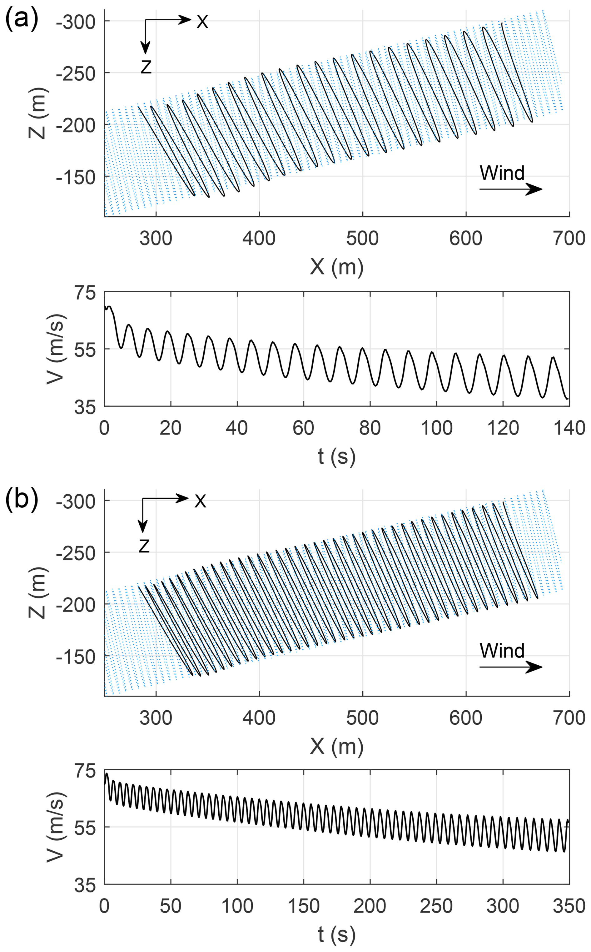
Figure 21 Reeling out at 2.5 m s⁻¹ (a) and 1.0 m s⁻¹ (b) winch speed, showing lower airspeed in (a) due to faster reel out.

By the same token, flying in lower wind speeds can be done by reducing the winch speed accordingly. The KM1 airframe stalls at 20 m s⁻¹ airspeed, so the minimum acceptable airspeed during simulated reel out in steady uniform wind was chosen to be 30 m s⁻¹. This apparently large margin is deemed necessary because steady and uniform wind is rarely encountered in real flights, so the kite must be able to remain airborne during temporal drops in wind speed. This airspeed constraint results in a reel-out winch speed of zero in 8 m s⁻¹ uniform wind. Figure 10 shows the resulting trajectory: a circular orbit with the winch locked in place to keep the tether length fixed at 350 m – arguably a fixed-wing version of “parking” the kite mid-air as seen in soft kites AWES but achievable at much lower wind speeds (Fechner et al., 2015). The minimum airspeed is reached at the top of the circle. Therefore, preventing such a large drop in airspeed will enable the kite to operate at lower wind speeds. One method to do so is to phase-synchronise winch speed control with flight control. This winch control method can reduce the KM1's “minimum parking wind speed” to 6.7 m s⁻¹, thereby enabling power production in 8 m s⁻¹ wind. Further details of such a winch control system will be provided in a future publication. In the context of this paper, we have shown that the flight control system can track the target cylinder as long as there is sufficient airspeed to prevent stall.

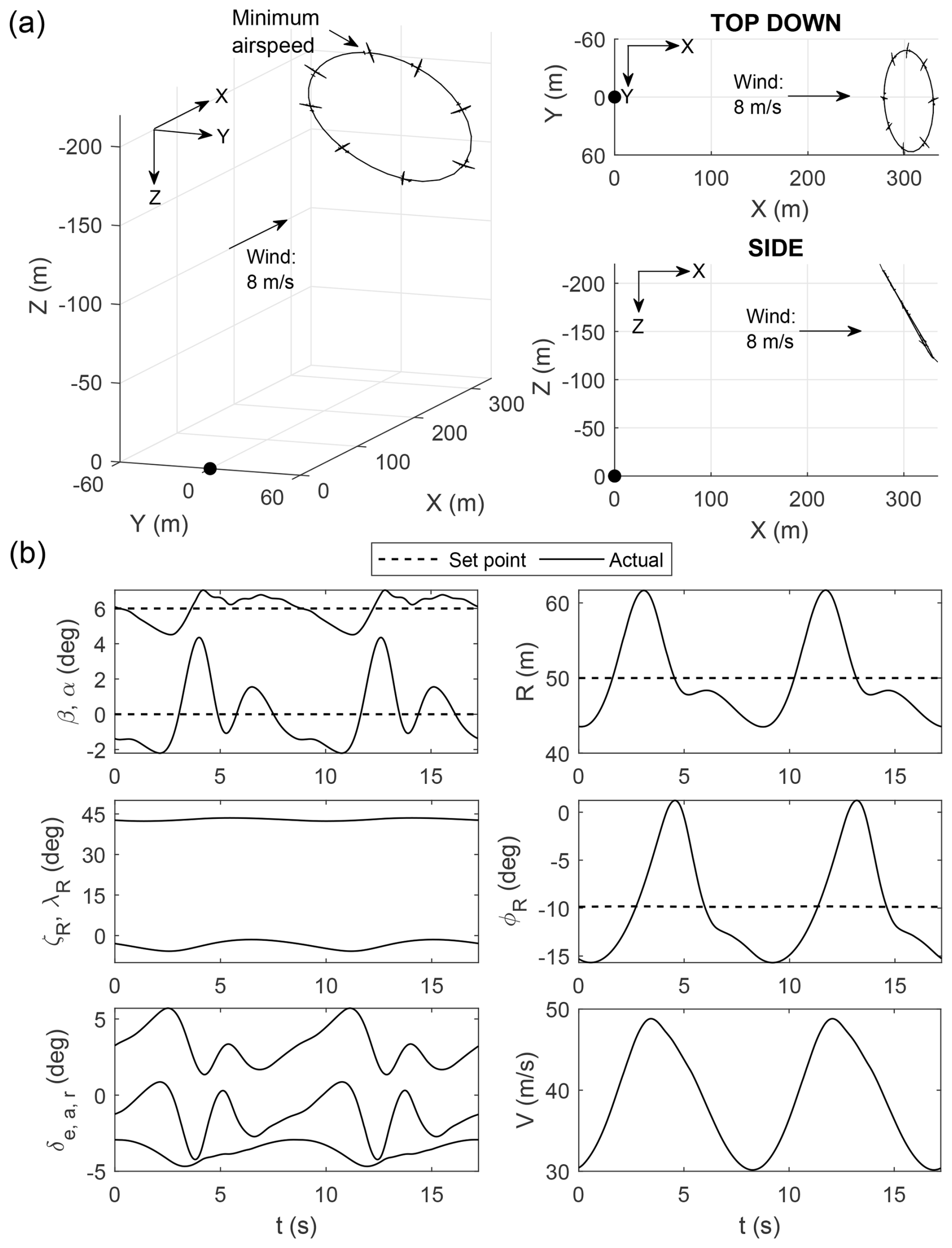
Figure 22 Trajectory under zero winch speed in 8 m s⁻¹ wind. The kite is drawn true to scale at 1 s intervals. Time histories show data from two cycles.

5.2 Radius control with large error signal

Figure 23a shows the kite joining a sideway reel out from outside the target cylinder. A bottleneck point is seen, which is caused by the radius controller. At the starting point, the radius error is large, so the radius tracker tightens the turn to compensate for the large error signal. This manoeuvre can excessively reduce the radii of the enroute circular loops, causing potential control problems. To avoid the bottleneck problem, radius control should be turned off until the kite is already inside the target cylinder. Figure 23b shows the kite rejoining the same cylinder but with ${\mathit{\varphi }}_{{\mathrm{R}}_{\mathrm{SP}}}$ manually set to −3° at the start, which resulted in no bottleneck. Once inside the cylinder, radius tracking can be safely turned on.

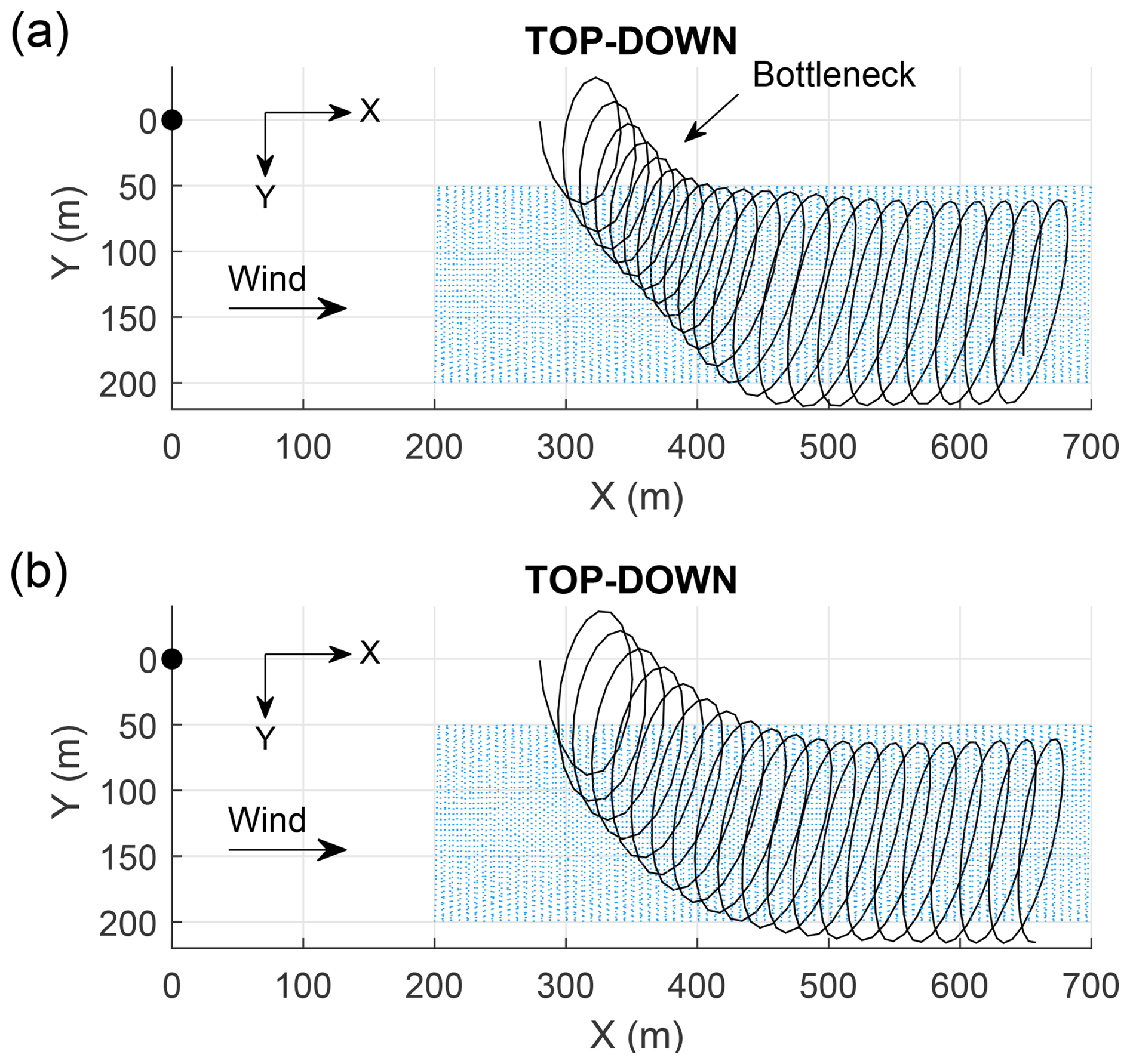
Figure 23 Bottleneck issue caused by enabling radius tracking when the kite is far outside the cylinder: (a) with radius tracking deployed, (b) without radius tracking.

5.3 Cosine losses at high altitudes

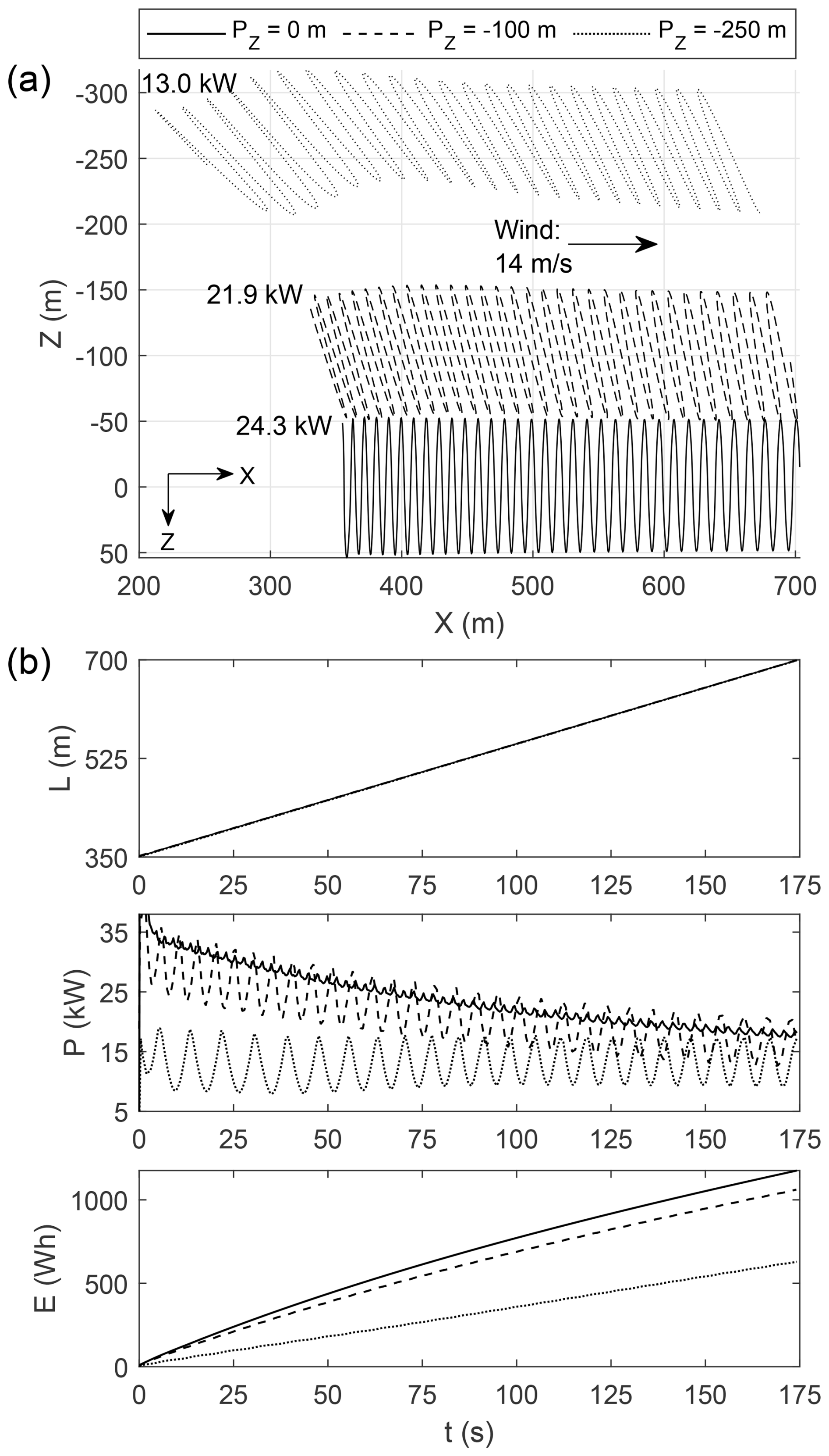
Early AWES literature has noted the cosine loss phenomenon, where given the same wind speed, power is reduced at higher altitudes (Diehl, 2013). This reduction is caused by a misalignment between the aerodynamic force and the wind vector. In the context of circular reel out, flying higher means individual orbits are angled further away from their ideal position of being 90° to the wind. The misalignment between aerodynamic force and wind direction increases, resulting in power reduction. A demonstration is provided in Fig. 24, which analyses three horizontal reel-out trajectories with same radii (50 m) but different target heights (reflected by different values for P_z, which is the Z coordinate of the target cylinder's origin in the Earth axis).

• Solid line: ideal trajectory orbiting the centre of the wind window with P_z=0 m and no gravity. This flight path is not achievable in test flights due to the negative heights.

• Dashed line: 100 m height with gravity. This trajectory can be considered realistic.

• Dotted line: 250 m height with gravity.

The kite with highest altitude experiences more control difficulty, and notably produces 46 % less power than in the ideal case. As altitude increases, the angle between individual circular orbits and the wind drops below the ideal value of 90°, which is achieved only when P_z=0 m with no gravity. Due to this increasing misalignment with height, the wind contributes less to pulling the tether out, resulting in less power generated. Whilst flying higher also increases tether drag and reduces power, the contribution from the cosine loss is more significant. If the kite at $P_z=-\mathrm{250}$ m was to achieve 21.9 kW (same power output as with $P_z=-\mathrm{100}$ m), the wind speed must increase to 17 m s⁻¹.

Figure 24 Different power production capacities at different heights due to cosine loss.

5.4 Minimum viable controller: ailerons only

Since all outer-loop signals are combined into just one control surface input (ailerons – see Fig. 12), the kite can follow the target cylinder with elevator and rudder fixed. Figure 25 shows one such example, where rudder is kept neutral and elevator is set to −4°. Power production is less efficient without active angle of attack and sideslip monitoring, but being able to test the flight controller without pitot tubes (for α and β measurements) can be useful for rapid development of new AWES prototypes. Mathematically speaking, flying with only one active control surface is possible because the goal of tracking a constant radius – regardless of the flight path taken – is a one-degree-of-freedom problem. This formulation of feedback control reduces complexity and implies that a different control effector can be used. Indeed, test flights at Kitemill have successfully flown circular reel out using only rudder (ailerons and elevator are fixed), although simulations show that this method is less efficient for power generation than using ailerons (Nguyen et al., 2026a).

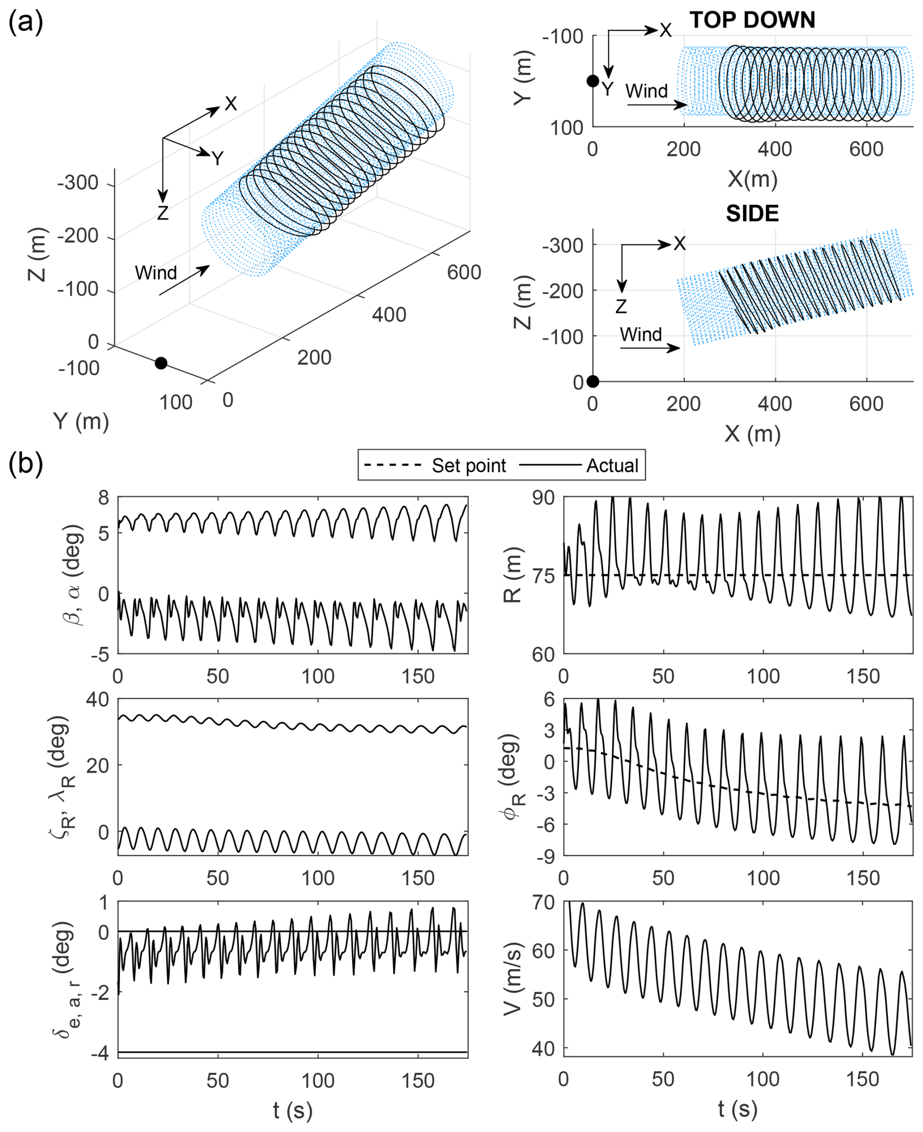
Figure 25 Normal reel out flown with fixed elevator (−4°) and rudder (0°). Parameters: $\mathbf{P}=[\mathrm{200},\mathrm{0},-\mathrm{150}]$ m, [λ_P, ${\mathit{\zeta }}_{\mathrm{P}}]=[\mathrm{13}\mathit{°},\mathrm{0}\mathit{°}]$, and R_SP=75 m. The winch speed is kept constant at 2.0 m s⁻¹.

5.5 Semi-manual mode

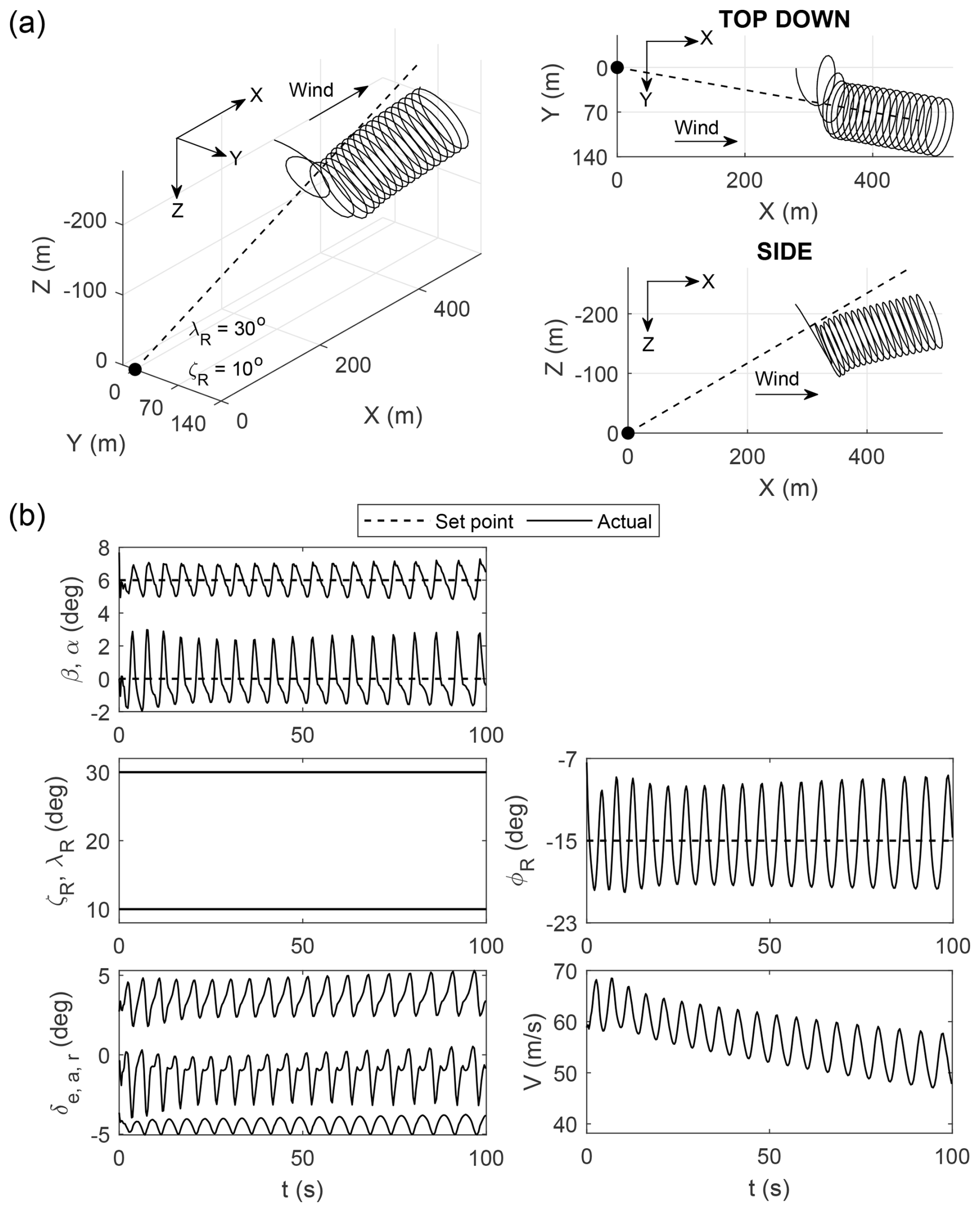
The kite can be flown using only the inner loop – even with the winch active. We refer to this configuration as the “semi-manual mode”. Figure 26 shows an example. Five set points have to be specified by the user as shown in Fig. 7, namely ${\mathit{\varphi }}_{R_{\mathrm{SP}}}$, λ_R, and ζ_R for the ailerons, α_SP for the elevator, and β_SP for the rudder (noting that the last two can also be kept fixed as discussed in Sect. 5.4). With λ_R sufficiently high for satisfactory ground clearance and ζ_R not too far off the wind direction, the kite can sustain safe circular reel out. Steering the reel-out path can be achieved by manually adjusting λ_R and ζ_R, while radius adjustment can be done with ${\mathit{\varphi }}_{R_{\mathrm{SP}}}$.

For initial AWES control development, we recommend flying in semi-manual mode with the tether length fixed, gravity disabled, and λ_R and ζ_R set to 0°. Doing so enable the kite to converge to an equilibrium state by circling a point at zero height. From here, the α_SP, β_SP, and ${\mathit{\varphi }}_{R_{\mathrm{SP}}}$ loops can be tuned using classical methods.

Figure 26 Semi-manual flight using only the inner loop.

5.6 Limit cycles

A potential downside of the controller is that it cannot converge to an equilibrium. To demonstrate, consider the full flight control system in a gravity-free environment with [λ_P, ${\mathit{\zeta }}_{\mathrm{P}}]=[\mathrm{0}\mathit{°},\mathrm{0}\mathit{°}]$ and fixed tether length as shown in Fig. 27a. The resulting circular trajectory is perpendicular to the wind, and past work has shown that an equilibrium trim point exists in this condition (i.e. no cyclic control surface movement required) (Nguyen et al., 2026b). However, Fig. 27b shows that λ_R and ζ_R still exhibit small limit cycles caused by the integrated production-plane coordinates X_P and Y_P in the error signal. All three control surfaces are also in limit cycles as a result. These limit cycles disappear when λ_R and ζ_R are manually set to zero, at which point, the kite can be linearised for inner-loop control design. For the outer loop, the small-amplitude limit cycles can be ignored during manual tuning, but they may pose a challenge for rigorous control design. Further discussions on analysing nonlinear limit-cycle systems can be found in maths textbooks such as Jordan and Smith (2007).

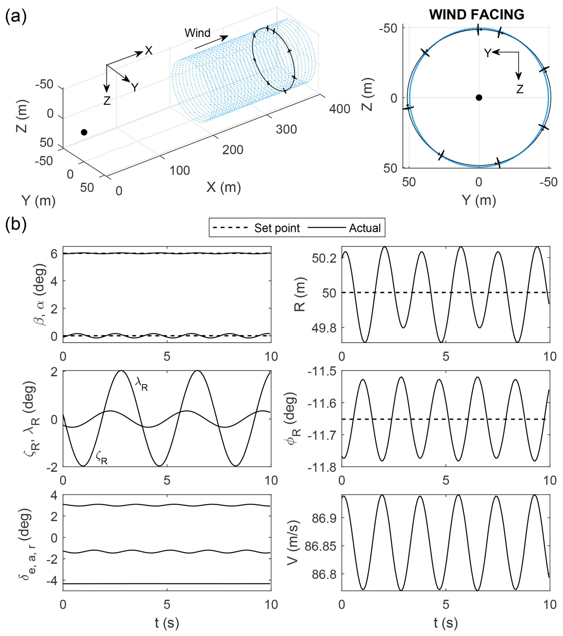
Figure 27 Closed-loop limit cycles, which is always present in the full flight controller even when equilibrium trim is possible.

6 Control law extensions

6.1 Reducing angle-of-attack oscillation

Although limit cycles cannot be eliminated, some can be reduced in amplitude. Angle of attack is one prime candidate for this reduction because flying at a near-constant α keeps the airframe close to its optimal aerodynamic configuration, which improves power generation. Two elements contribute to angle-of-attack oscillation during circular reel out: changing apparent wind direction at different points in the circle and changing gravity direction with respect to the airframe's body axis. Whilst the former is unavoidable, the latter can be reduced. Assuming no external wind, gravity's contribution can be seen in the last term of Eq. (12).

$$\begin{array}{}\text{(12)}& \begin{array}{rl}\dot{\mathit{\alpha }}& =q-{\displaystyle \frac{\mathrm{1}}{\mathrm{2}}}{\displaystyle \frac{\mathit{\rho }\mathrm{VS}}{m}}{C}_{\mathrm{L}}-\left(p\cos \mathit{\alpha }+r\sin \mathit{\alpha }\right)\tan \mathit{\beta }\\ & +{\displaystyle \frac{g}{V}}\left({\displaystyle \frac{\cos \mathit{\varphi }\cos \mathit{\theta }\cos \mathit{\alpha }+\sin \mathit{\theta }\sin \mathit{\alpha }}{\cos \mathit{\beta }}}\right)\end{array}\end{array}$$

This is one of the standard six-degree-of-freedom equations of motion for aircraft but is written in the aerodynamic wind axis (α,β, V) instead of the more common body-axis velocities (u, v, w). If the contribution of gravity in Eq. (12) can be cancelled out using feedback control, angle-of-attack oscillation will be significantly reduced. This gravity term can be decomposed into two components:

$$\begin{array}{}\text{(13)}& {\displaystyle }{\dot{\mathit{\alpha }}}_{g_z}={\displaystyle \frac{g}{V}}{\displaystyle \frac{\cos \mathit{\varphi }\cos \mathit{\theta }\cos \mathit{\alpha }}{\cos \mathit{\beta }}},\text{(14)}& {\displaystyle }{\dot{\mathit{\alpha }}}_{g_x}={\displaystyle \frac{g}{V}}{\displaystyle \frac{\sin \mathit{\theta }\sin \mathit{\alpha }}{\cos \mathit{\beta }}},\end{array}$$

where ${\dot{\mathit{\alpha }}}_{g_z}$ describes how the body-axis (not Earth-axis) vertical component of gravity affects angle of attack, and ${\dot{\mathit{\alpha }}}_{g_x}$ reflects the contribution of the longitudinal component. Comparing both variables against α in Fig. 28, one can see that ${\dot{\mathit{\alpha }}}_{g_x}$ is roughly in phase with α and oscillates about zero, whereas ${\dot{\mathit{\alpha }}}_{g_z}$ has a slight phase lead and is offset from zero. Both properties of ${\dot{\mathit{\alpha }}}_{g_x}$ suggest that it can be used as a feedback signal on the elevator channel to cancel out the angle-of-attack oscillation. This is possible in the simulation. However, ${\dot{\mathit{\alpha }}}_{g_x}$ in Eq. (14) has three quantities that require measurements from a pitot tube: V, α, and β. If all three are removed from Eq. (14), the right-hand side reduces to just gsin θ. Figure 28 shows that this term has similar phase and offset properties as the full ${\dot{\mathit{\alpha }}}_{g_x}$ equation. Therefore, the feedback signal to the elevator can be simply K_gsin θ, where K_g is a proportional gain equal to g multiplied by a constant. This additional feedback path creates the second junction in the elevator path (see Fig. 12). As such, the augmented pitch control law is

$$\begin{array}{}\text{(15)}& {\mathit{\delta }}_{{\mathrm{e}}_{\mathrm{SP}}}=\mathrm{PI}({\mathit{\alpha }}_{\mathrm{SP}},\mathit{\alpha })+K_g\sin \mathit{\theta }.\end{array}$$

Figure 28 Potential feedback terms to cancel out the effect of gravity on α oscillation.

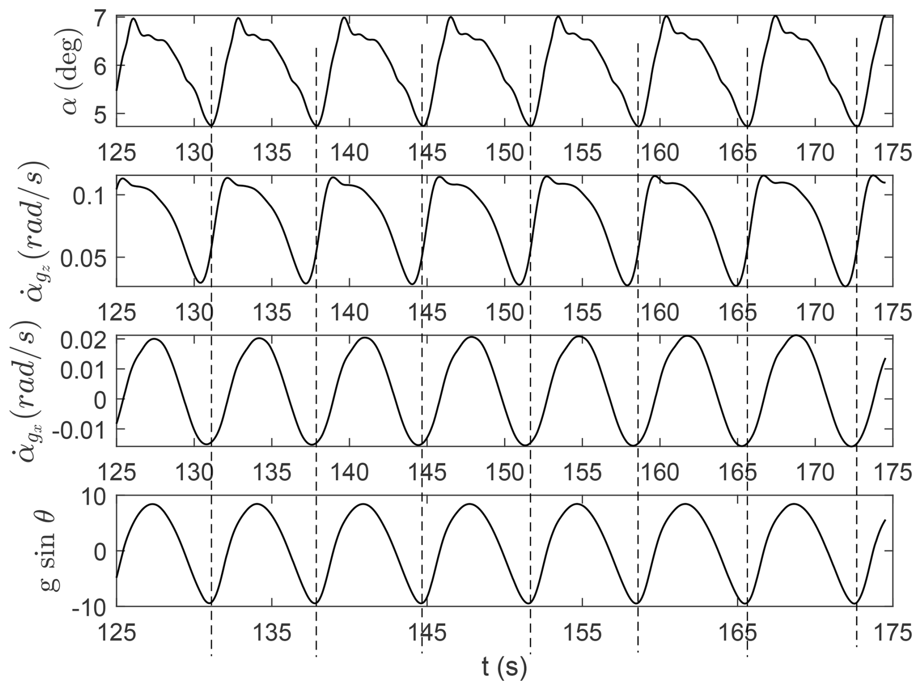
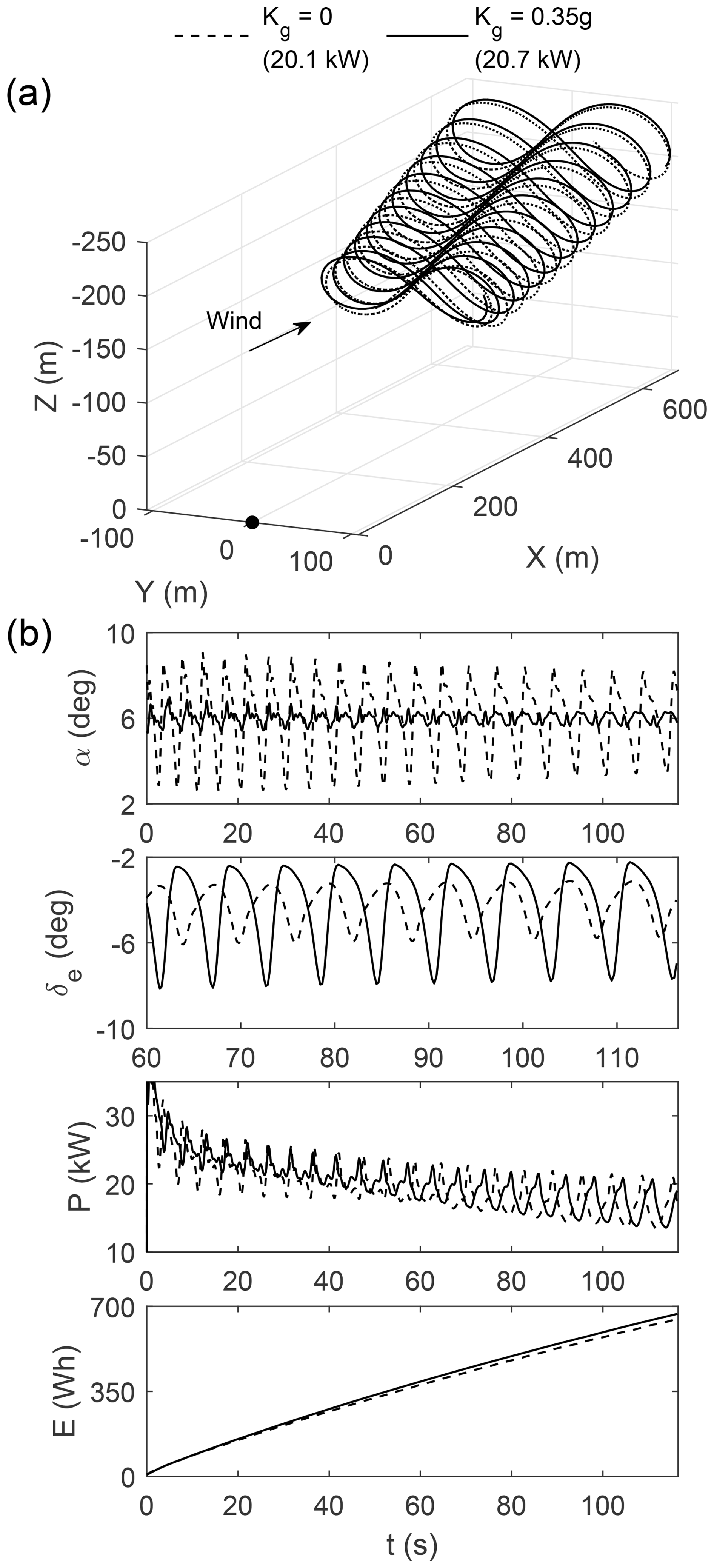
Figure 29 shows the effect of the new pitch control law on angle of attack and power generation over a normal reel-out trajectory but with a low radius of 50 m to exaggerate α oscillation. The dashed line labelled “K_g=0” indicates flying without the α-suppression controller. It can be seen that the controller successfully suppresses the limit cycle in α and provides a marginal 0.1 kW gain in power. This power gain is more noticeable if a less ideal winch is used. In Fig. 30, the same reel-out trajectory is flown again but with a winch that maintains a constant tether tension of 8 kN. This winch control mechanism is less efficient for power generation (Nguyen et al., 2026a) but is closer to what has been tested experimentally at Kitemill. In this arrangement, angle of attack oscillation has been significantly reduced. The kite experiences less aerodynamic drag as a result and completes the production cycle 14 s faster – a 0.9 kW gain in power. Inspecting the elevator movement in both Figs. 29 and 30, we can see that the new pitch control law has phase-shifted the cyclic elevator input and also demands more elevator movements compared to the K_g=0 case, resulting in the desired α-suppression effect. This behaviour reflects the fact that our proposed control law is a form of dynamic inversion.

Figure 29 Effect of the α-suppression controller. The winch speed is constant at 2 m s⁻¹.

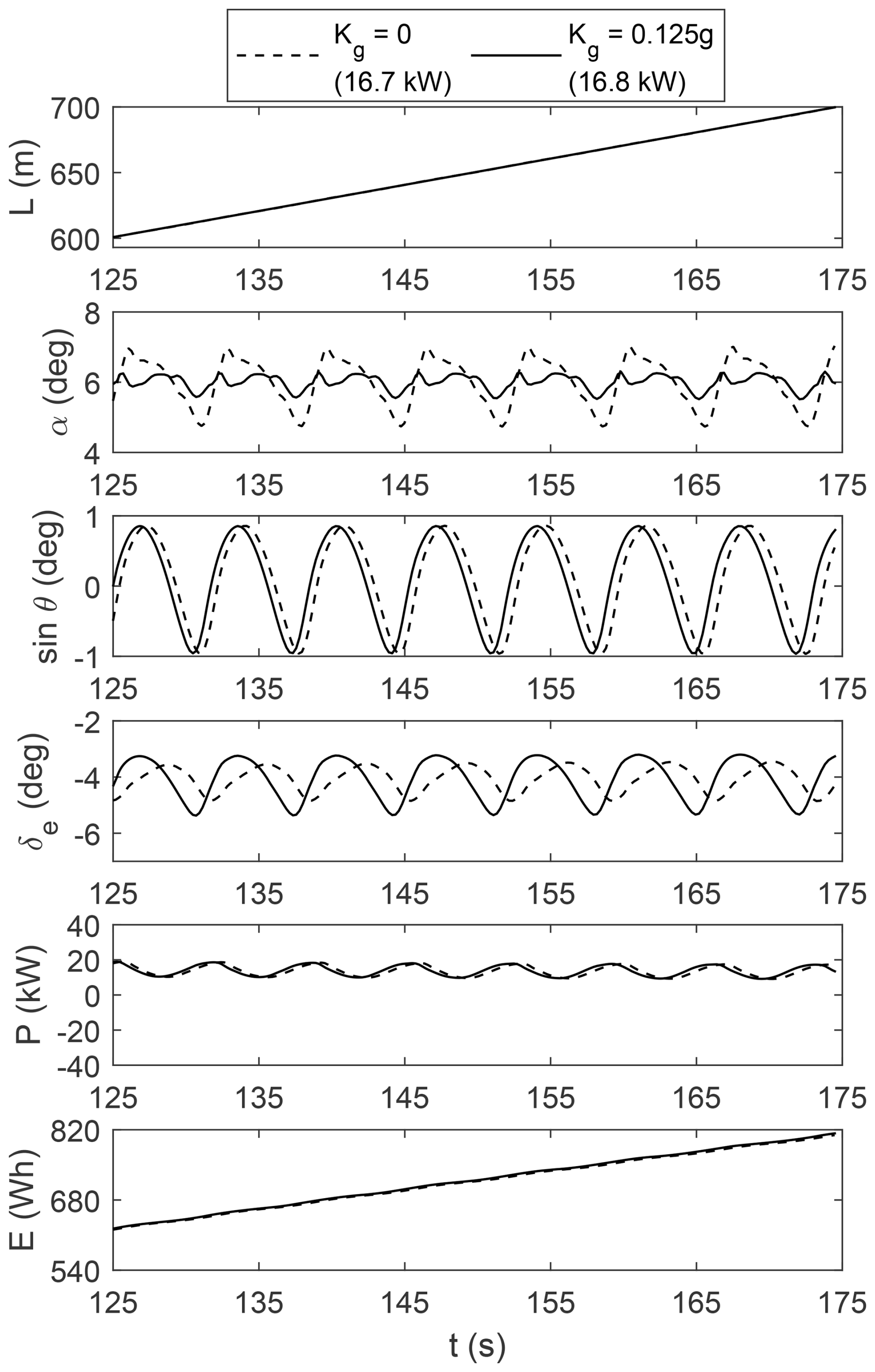
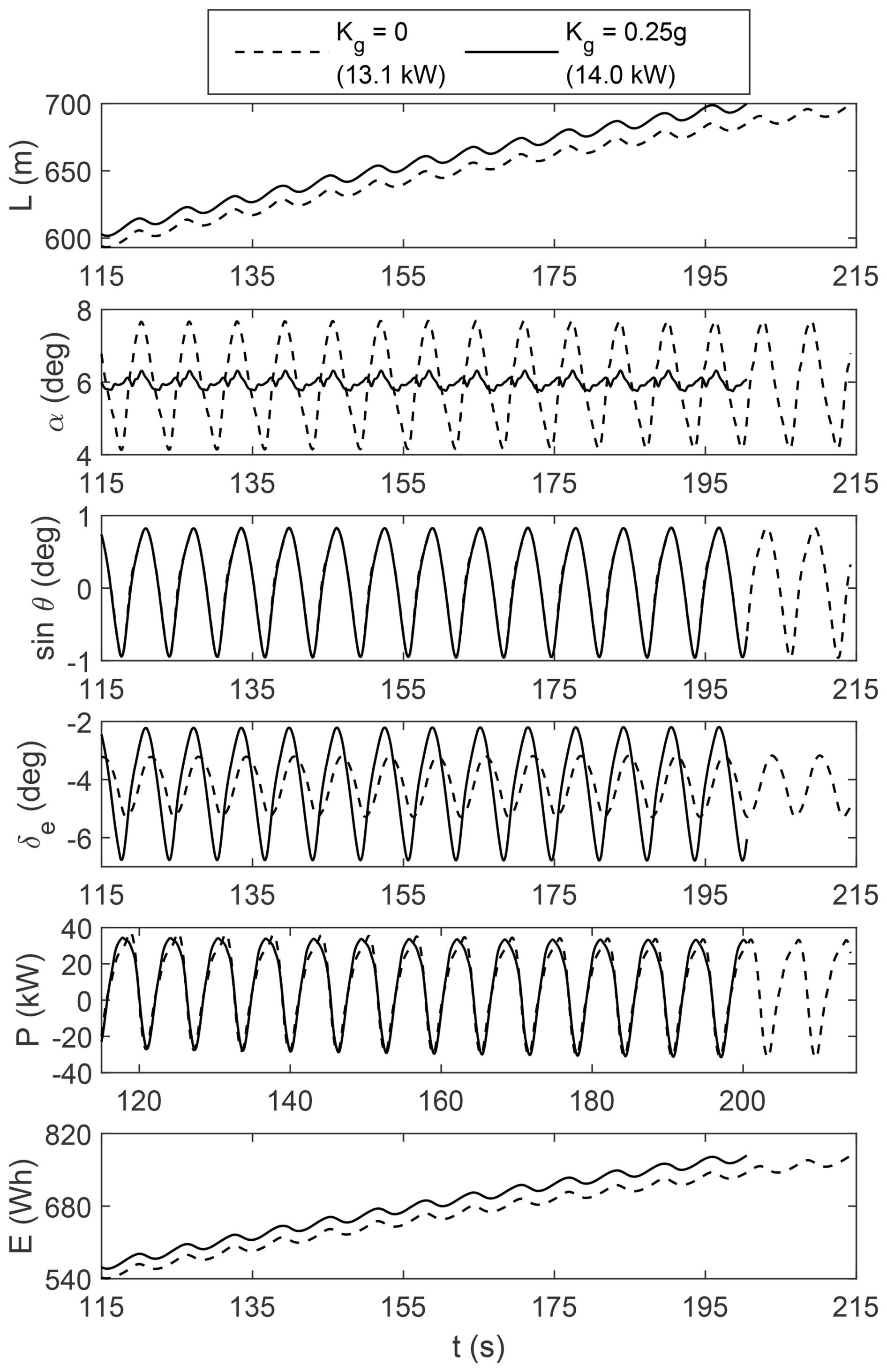
Figure 30 Effect of the α-suppression controller. The winch tracks a constant tether tension of 8 kN.

Figure 31 Starting location of the two kites for synchronisation testing.

Since gravity's contribution is independent of the chosen flight path, the angle-of-attack suppression controller also works with figure-of-eight reel out. This capability is demonstrated in Sect. 6.3. Appendix C presents the stability proof of the α dynamics in closed loop with the proposed controller.

6.2 Multi-kite synchronisation

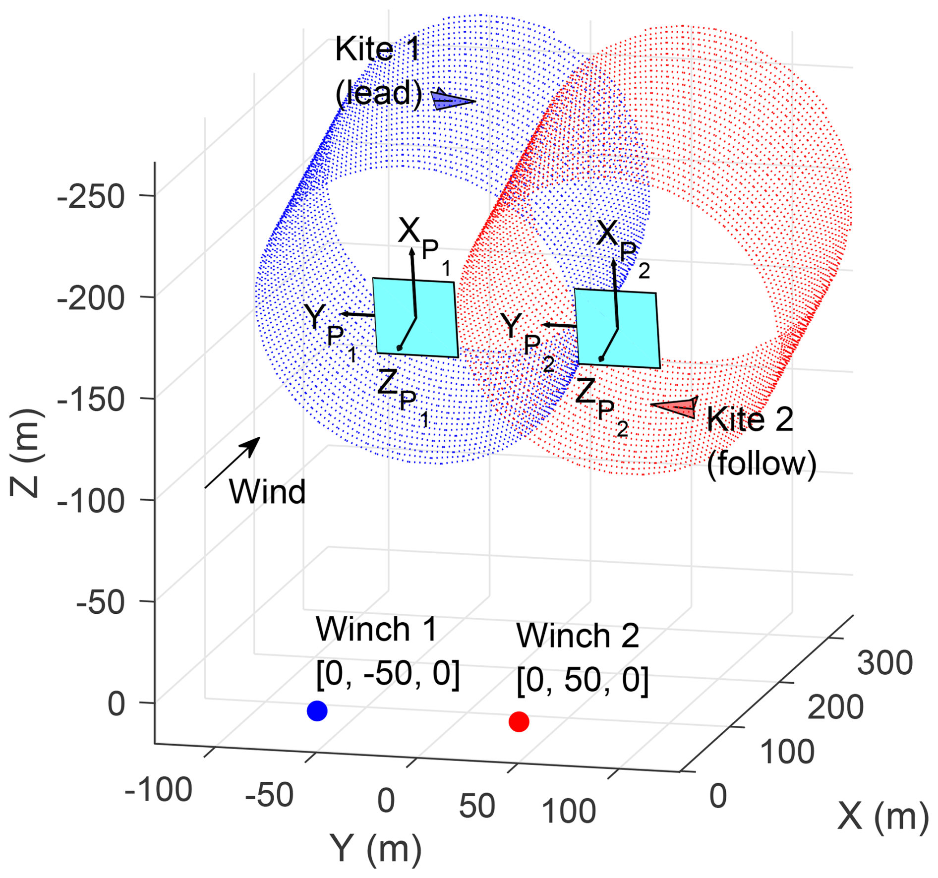
Our proposed flight controller can be extended to synchronise multiple kites in a farm configuration, where a minimum separation rule may be in place. The working principle is based on the fact that without a dedicated propulsion unit, the kite's angular velocity in the cylinder is dependent primarily on radius. Faster sweep is achieved by lowering the radius and vice versa, as shown in Fig. 10. Within the same 10 s window, the blue trajectory with a smaller radius completes around 2.5 orbits, whereas the grey one does only 1.5. Therefore, phase synchronisation of multiple kites can be achieved by adjusting the radius. To demonstrate, consider a hypothetical two-kite farm scenario in Fig. 31. Two target cylinders with 80 m radius are placed with only 100 m in lateral separation between their centre lines, leading to 60 m of overlap in the Y direction. The angular phase Ω of each kite in its target cylinder is defined as

$$\begin{array}{}\text{(16)}& \mathrm{\Omega }=\mathrm{atan}\mathrm{2}\left(Y_{\mathrm{P}},X_{\mathrm{P}}\right).\end{array}$$

Note that Ω=0° corresponds to the kite being at the highest point of the circle.

Figure 32 Phase synchronisation controller in the second kite.

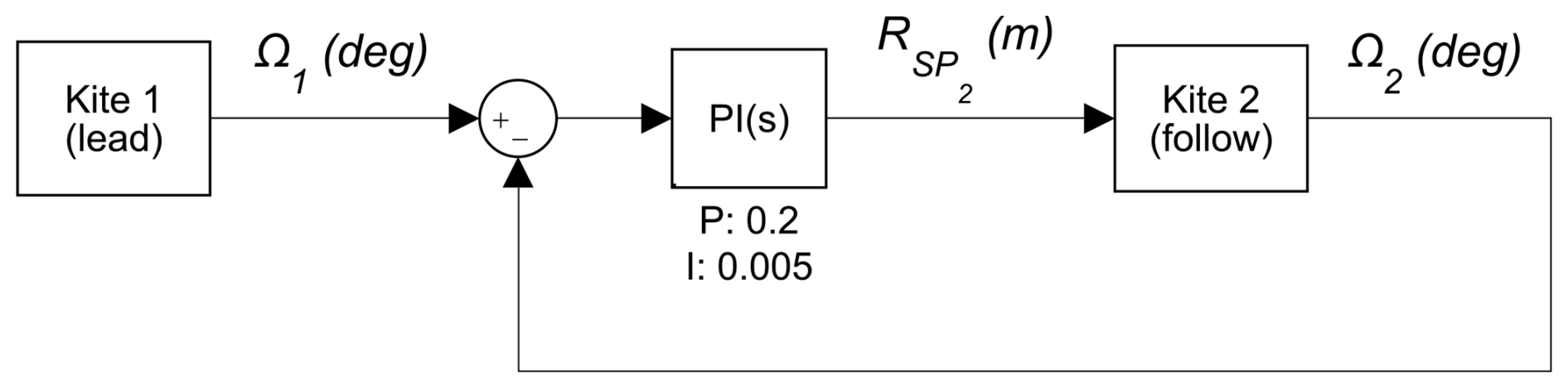
The lead kite is flown normally using the control scheme in Fig. 12. For the second kite, the radius set point $R_{{\mathrm{SP}}_{\mathrm{2}}}$ is automatically adjusted using an additional PI loop presented in Fig. 32. This controller seeks to match the second kite's phase with the first kite's by adjusting the second kite's radius. To prevent overcorrection, the output $R_{{\mathrm{SP}}_{\mathrm{2}}}$ of the phase-synchronisation controller is limited to between 60 and 100 m, which is no more than ±20 m from $R_{{\mathrm{SP}}_{\mathrm{1}}}=\mathrm{80}$ m.

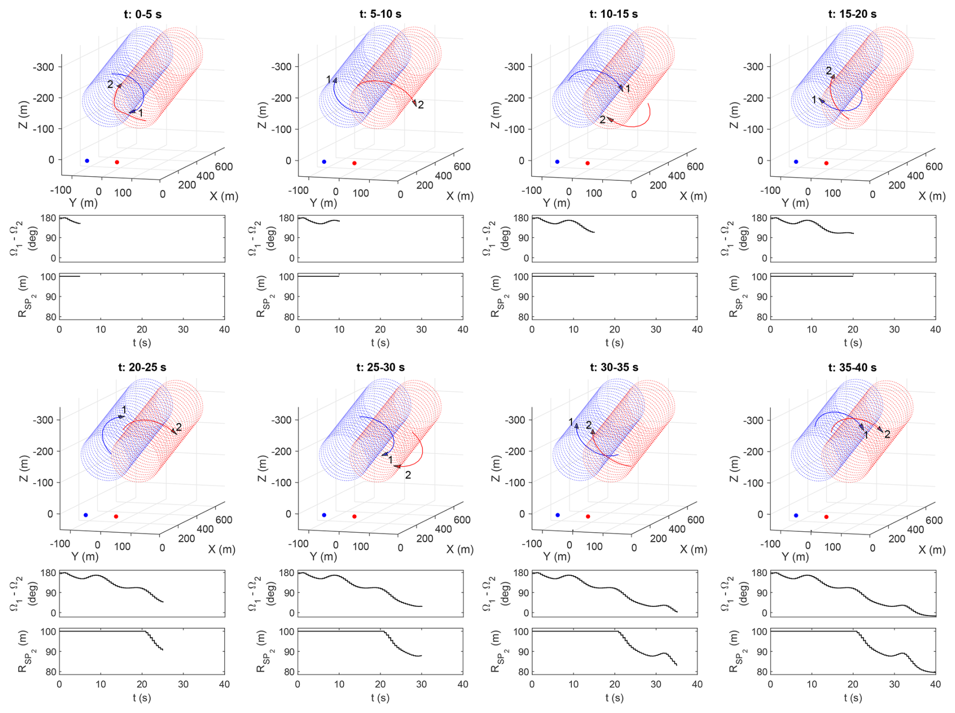
The phase synchronisation controller is now tested with two kites starting from a 180° out-of-phase position as shown in Fig. 31. Longitudinal separation is provided by the different starting tether lengths: 350 m for kite 1 and 300 m for kite 2. The resulting trajectories in Fig. 33 show successful synchronisation after 35 s, or just under three loops. Once the phase gap is closed, the second kite remains in sync for the rest of the reel-out cycle.

Figure 33 Simulation result of the phase synchronisation controller.

6.3 Figure-of-eight flight pattern

The proposed control framework can be adapted to fly figure-of-eight (henceforth abbreviated to “F8”) patterns using a proportional feedback law. Although this method cannot provide non-symmetric flight capabilities as seen in circular-flight analysis (i.e. sideway and diagonal reel out), it is sufficient as a demonstrator for rapid simulator development and verification. Consider a generic F8 pattern as shown in Fig. 34a. The production plane location is now shifted to the winch at the origin with the elevation and azimuth angles λ_P and ζ_P set to zero. In this configuration, the axis Z_P points in the opposite direction of the wind. Using the same definition of angular phase Ω from Eq. (6), we have the evolution of Ω over two F8 cycles as shown in Fig. 34b. This evolution resembles the amount of roll on the production plane required to fly an F8 path. Near the centre of lemniscate (point A), this roll angle crosses zero, reaching its peak positive and negative values at C or B (depending on whether an eight-up or eight-down pattern is flown). The phase angle Ω can therefore be used as the feedback signal to change the reference plane roll angle set point using a proportional control law with gain K₈

$$\begin{array}{}\text{(17)}& {\mathit{\varphi }}_{R_{\mathrm{SP}}}\left[\mathrm{deg}\right]=K_{\mathrm{8}}\mathrm{\Omega }\left[\mathrm{deg}\right],\end{array}$$

where the sign of the proportional gain K₈ determines if the trajectory is eight-up or eight-down. Setting a larger magnitude for K₈ means a tighter turn when the kite reaches the edge of the lemniscate, resulting in a narrower F8 trajectory. The aileron control law requires a minor modification:

$$\begin{array}{}\text{(18)}& {\mathit{\delta }}_{{\mathrm{a}}_{\mathrm{SP}}}=\mathrm{PI}\left({\mathit{\varphi }}_{{\mathrm{R}}_{\mathrm{SP}}},{\mathit{\varphi }}_{\mathrm{R}}\right)+K_{\mathrm{r}}{\mathit{\theta }}_{\mathrm{r}}{K}_{\mathrm{s}}{\mathit{\varphi }}_{{\mathrm{R}}_{\mathrm{SP}}},\end{array}$$

noting that the roll stiffness term is now multiplied by a factor $K_{\mathrm{s}}{\mathit{\varphi }}_{{\mathrm{R}}_{\mathrm{SP}}}$, with K_s being another proportional gain. This addition accommodates the fact that the roll stiffness gain K_r must change sign depending on which side of the lemniscate the kite is flying on. Because ${\mathit{\varphi }}_{{\mathrm{R}}_{\mathrm{SP}}}$ has a smooth zero crossing near centre of the lemniscate, this signal can be used to indicate sign change after appropriate scaling by K_s to keep the peak magnitude of $K_{\mathrm{s}}{\mathit{\varphi }}_{{\mathrm{R}}_{\mathrm{SP}}}$ close to 1. In all subsequent results, K_s is fixed at −0.05. Figure 35 shows the block diagram of the F8 controller. The only user input available (beyond control gains) is the reference plane elevation angle λ_R. All other guidance parameters must be set to zero to avoid instability caused by the limited steering capability of the proportional control law, which requires symmetry in the lemniscate to function properly.

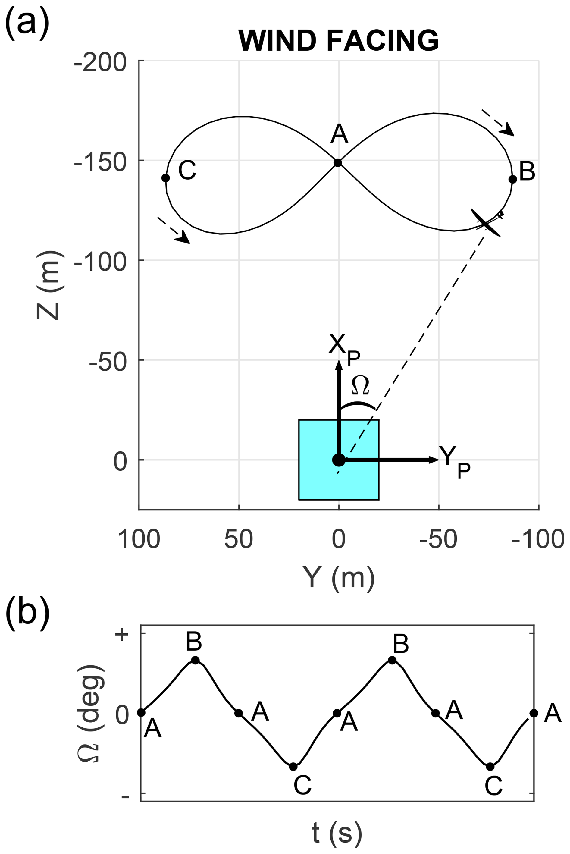
Figure 34 A generic figure-of-eight pattern (a) and evolution of the phase angle over two cycles (b).

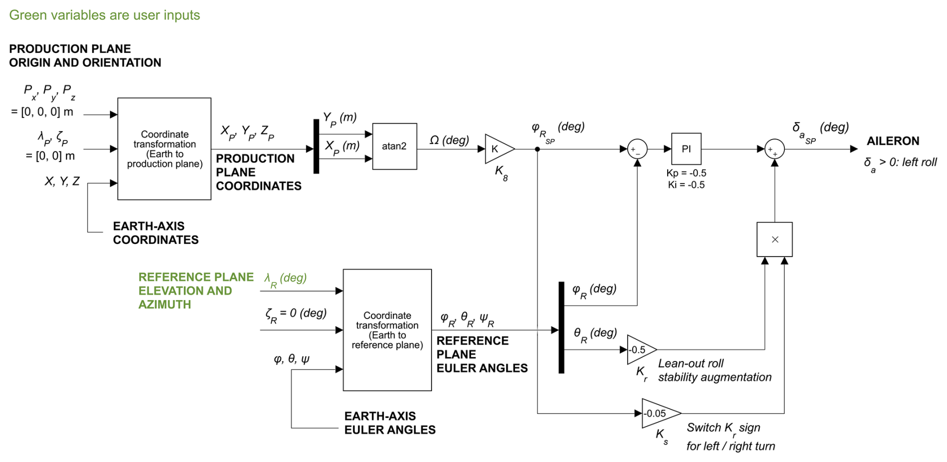
Figure 35 Block diagram of the figure-of-eight flight controller for aileron. Note that the elevator and rudder loops remain unchanged.

The controller's performance is now assessed. Figure 36 shows a few F8 patterns with positive and negative gains. As discussed, the lemniscate's width can be reduced by increasing K₈ magnitude. To fly at a higher elevation, λ_R should be increased as shown in Fig. 37.

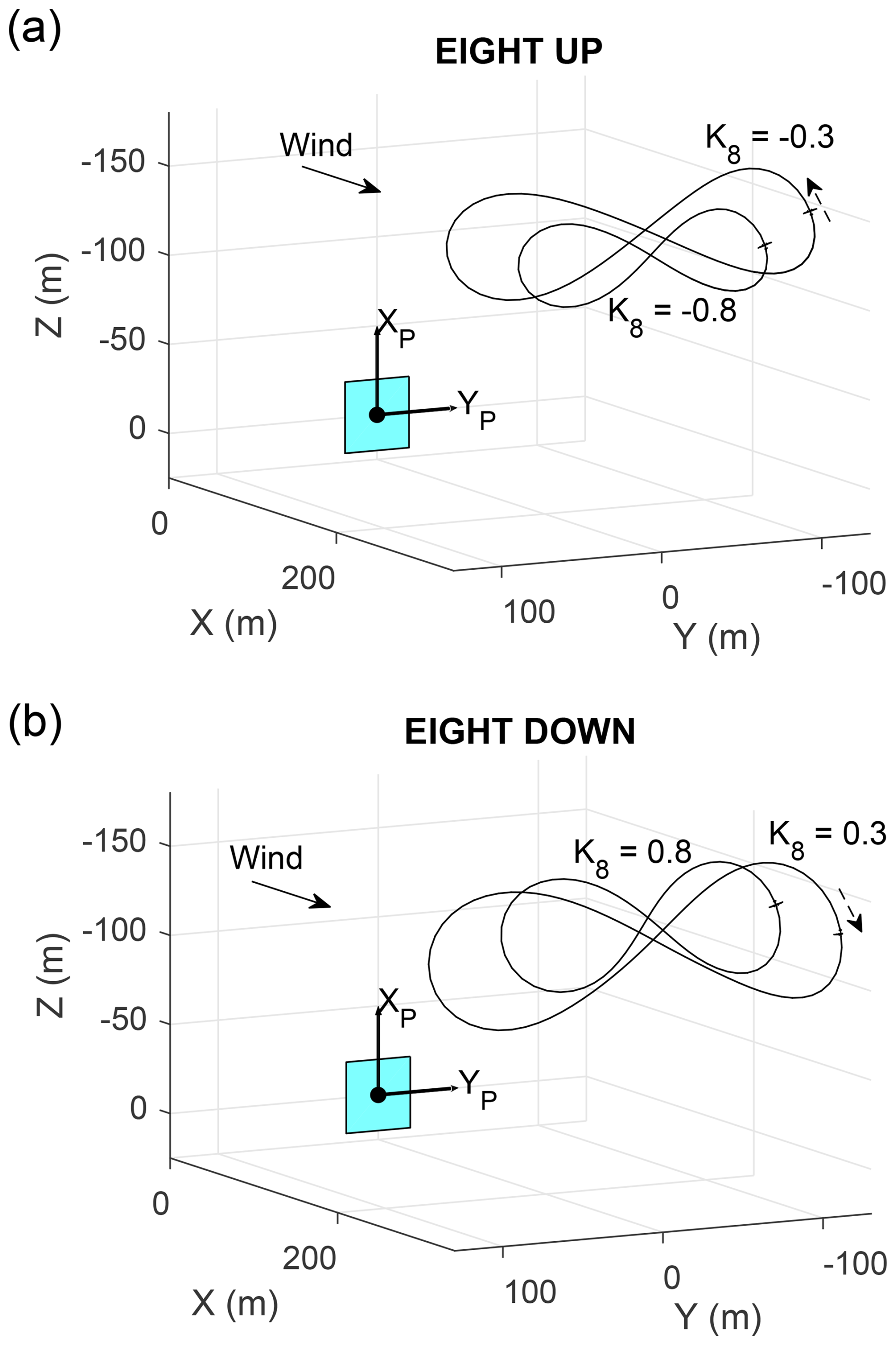
Figure 36 Eight-up (a) and eight-down (b) trajectories at λ_R=25° with different control gains.

Figure 37 Effect of changing λ_R.

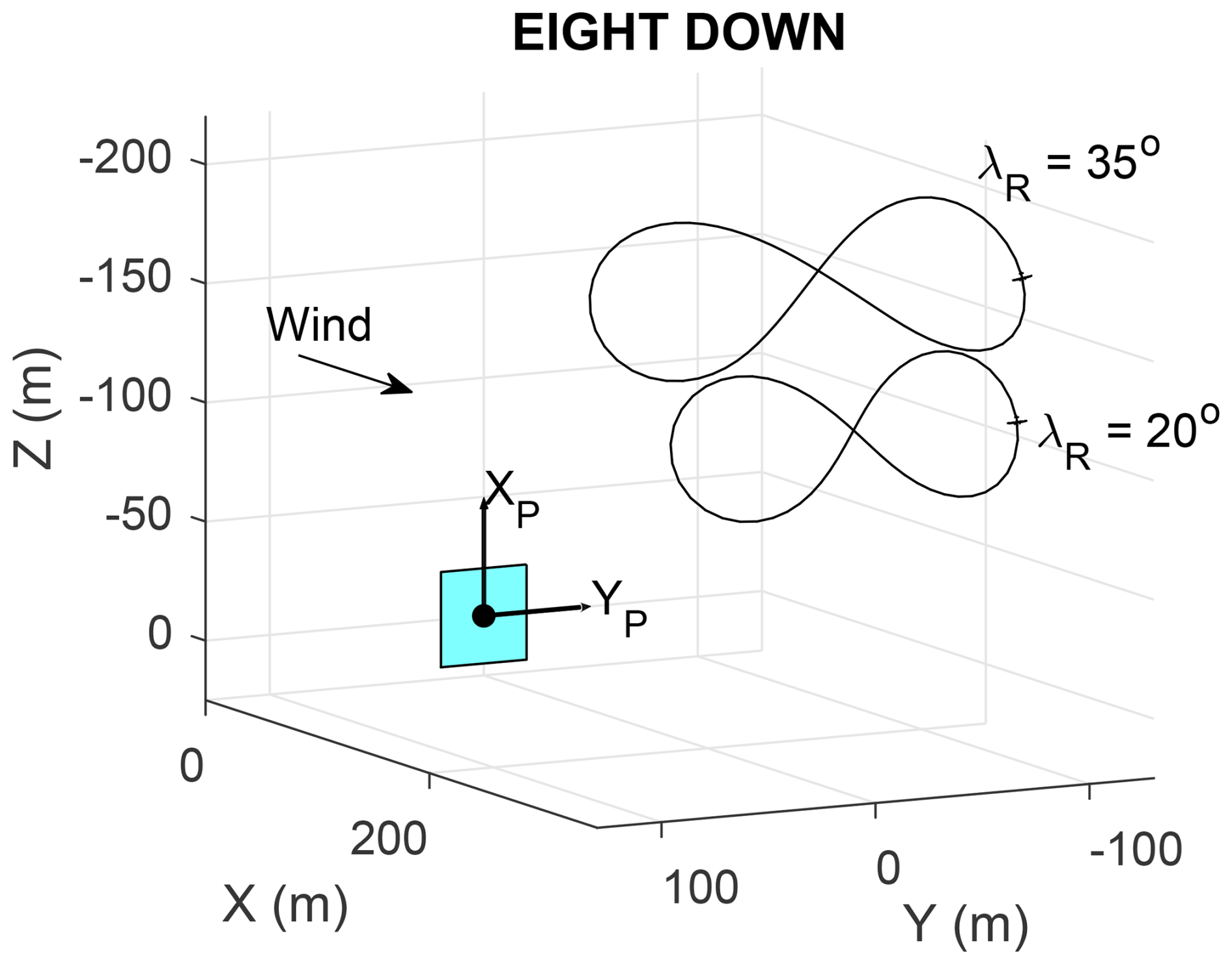
An F8 pattern can be considered to be two small circles on each side joined at the centre of the lemniscate. Each side-circle's radius is smaller than typical values for circular reel out. As a result, the angle of attack and sideslip variation can be large, although the former can be alleviated using the α-suppression controller in Eq. (15). Figure 38 demonstrate the controller's effectiveness in keeping α close to its 6° set point throughout a typical F8 reel-out cycle. This result confirms that the α-suppression controller can be used on both circular and figure-of-eight flight.

Figure 38 Eight-down reel out without and with α-suppression control.

7 Conclusions

This paper has shown that by relaxing the path-following requirement, a simple proportional-integral feedback system can provide accurate flight control during circular-pattern reel out. The key enabling idea is in tracking the roll angle on a non-static reference frame. In its simplest form, the controller achieves accurate path following using only ailerons while requiring no air data from a pitot tube. This capability could enable rapid control law development and testing of new AWES prototypes. Future improvements can implement more advanced controllers, such as nonlinear dynamic inversion, for the same roll-angle tracking idea but with higher performance. Additionally, recognising that AWES are self-oscillating systems opens up a new class of nonlinear controllers with great potential for the sector. An example of leveraging the inherent limit cycle property to improve performance is provided in the extension to the pitch control loop. By adding a proportional pitch angle feedback term to the elevator, angle-of-attack oscillation can be significantly reduced. Doing so enables the kite to spend more time in its optimal aerodynamic condition and results in more power. Lastly, an additional PI loop that adjusts circular flight radius provides indirect control of the kite's angular velocity. This property can be exploited to enable phase-synchronisation of multiple kites in a farm configuration. The proportional-integral architecture also positions the controller as a suitable baseline system for benchmarking more advanced control laws. All of the above developments contribute to making AWES safer and more efficient, thereby bringing them one step closer to commercial use.

Appendix A: Earth-to-reference-plane transformation

The Euler roll, pitch, and yaw angles on the reference plane [ϕ_R, θ_R, ψ_R] are obtained from their Earth-axis counterparts [ϕ, θ, ψ] and the reference plane's elevation and azimuth angles [λ_R, ζ_R]. This procedure is outlined in Eqs. (A1)–(A7). Subscripts E, B, and R denote Earth, body, and reference frames, respectively.

$$\begin{array}{}\text{(A1)}& {\displaystyle }\begin{array}{rl}{\mathbf{q}}_{\mathrm{EB}}& =\left[\begin{array}{l}\cos \left(\mathit{\psi }/\mathrm{2}\right)\\ \mathrm{0}\\ \mathrm{0}\\ \sin \left(\mathit{\psi }/\mathrm{2}\right)\end{array}\right]\otimes \left[\begin{array}{l}\cos \left(\mathit{\theta }/\mathrm{2}\right)\\ \mathrm{0}\\ \sin \left(\mathit{\theta }/\mathrm{2}\right)\\ \mathrm{0}\end{array}\right]\\ & \otimes \left[\begin{array}{l}\cos \left(\mathit{\varphi }/\mathrm{2}\right)\\ \sin \left(\mathit{\varphi }/\mathrm{2}\right)\\ \mathrm{0}\\ \mathrm{0}\end{array}\right],\end{array}\text{(A2)}& {\displaystyle }\begin{array}{rl}{\mathbf{q}}_{\mathrm{ER}}& =\left[\begin{array}{l}\cos \left({\mathit{\zeta }}_{\mathrm{R}}/\mathrm{2}\right)\\ \mathrm{0}\\ \mathrm{0}\\ \sin \left({\mathit{\zeta }}_{\mathrm{R}}/\mathrm{2}\right)\end{array}\right]\otimes \left[\begin{array}{l}\cos \left(\left({\mathit{\lambda }}_{\mathrm{R}}+\mathrm{90}\mathit{°}\right)/\mathrm{2}\right)\\ \mathrm{0}\\ \sin \left(\left({\mathit{\lambda }}_{\mathrm{R}}+\mathrm{90}\mathit{°}\right)/\mathrm{2}\right)\\ \mathrm{0}\end{array}\right]\\ & \otimes \left[\begin{array}{l}\cos \left(\mathrm{180}\mathit{°}/\mathrm{2}\right)\\ \sin \left(\mathrm{180}\mathit{°}/\mathrm{2}\right)\\ \mathrm{0}\\ \mathrm{0}\end{array}\right],\end{array}\text{(A3)}& {\displaystyle }{\mathbf{q}}_{\mathrm{BR}}={\mathbf{q}}_{\mathrm{EB}}^{-\mathrm{1}}\otimes {\mathbf{q}}_{\mathrm{ER}}=\left[\begin{array}{l}\mathit{\eta }\\ {\mathit{ϵ}}_{\mathrm{1}}\\ {\mathit{ϵ}}_{\mathrm{2}}\\ {\mathit{ϵ}}_{\mathrm{3}}\end{array}\right],\end{array}$$

where η, ϵ₁, ϵ₂, and ϵ₃ are the four elements in the 4 × 1 matrix q_BR. This gives a direction cosine matrix ${\mathbf{R}}_{\mathrm{R}}^{\mathrm{B}}$ of dimension 3 by 3

$$\begin{array}{}\text{(A4)}& {\mathbf{R}}_{\mathrm{R}}^{\mathrm{B}}=\mathbf{I}+\mathrm{2}\mathit{\eta }S\left(\mathit{ϵ}\right)+\mathrm{2}S\left(\mathit{ϵ}\right)S\left(\mathit{ϵ}\right),\end{array}$$

where $\mathit{ϵ}=\left[{\mathit{ϵ}}_{\mathrm{1}},{\mathit{ϵ}}_{\mathrm{2}},{\mathit{ϵ}}_{\mathrm{3}}\right]$ are the non-zero elements in the skew-symmetric matrix: S(ϵ)

$$\begin{array}{}\text{(A5)}& S\left(\mathit{ϵ}\right)=\left[\begin{array}{lll}\mathrm{0}& -{\mathit{ϵ}}_{\mathrm{3}}& {\mathit{ϵ}}_{\mathrm{2}}\\ {\mathit{ϵ}}_{\mathrm{3}}& \mathrm{0}& -{\mathit{ϵ}}_{\mathrm{1}}\\ -{\mathit{ϵ}}_{\mathrm{2}}& {\mathit{ϵ}}_{\mathrm{1}}& \mathrm{0}\end{array}\right].\end{array}$$

Substitute Eq. (A5) into Eq. (A4) and expand

$$\begin{array}{}\text{(A6)}& \begin{array}{rl}{\mathbf{R}}_{\mathrm{R}}^{\mathrm{B}}& =\left[\begin{array}{lll}{R}_{\mathrm{R},\mathrm{11}}^{\mathrm{B}}& R_{\mathrm{R},\mathrm{12}}^{\mathrm{B}}& R_{\mathrm{R},\mathrm{13}}^{\mathrm{B}}\\ R_{\mathrm{R},\mathrm{21}}^{\mathrm{B}}& R_{\mathrm{R},\mathrm{22}}^{\mathrm{B}}& R_{\mathrm{R},\mathrm{23}}^{\mathrm{B}}\\ R_{\mathrm{R},\mathrm{31}}^{\mathrm{B}}& R_{\mathrm{R},\mathrm{32}}^{\mathrm{B}}& R_{\mathrm{R},\mathrm{33}}^{\mathrm{B}}\end{array}\right]\\ & =\left[\begin{array}{lll}\mathrm{1}-\mathrm{2}({\mathit{ϵ}}_{\mathrm{2}}^{\mathrm{2}}+{\mathit{ϵ}}_{\mathrm{3}}^{\mathrm{2}})& \mathrm{2}({\mathit{ϵ}}_{\mathrm{1}}{\mathit{ϵ}}_{\mathrm{2}}-\mathit{\eta }{\mathit{ϵ}}_{\mathrm{3}})& \mathrm{2}({\mathit{ϵ}}_{\mathrm{1}}{\mathit{ϵ}}_{\mathrm{3}}+\mathit{\eta }{\mathit{ϵ}}_{\mathrm{2}})\\ \mathrm{2}({\mathit{ϵ}}_{\mathrm{1}}{\mathit{ϵ}}_{\mathrm{2}}+\mathit{\eta }{\mathit{ϵ}}_{\mathrm{3}})& \mathrm{1}-\mathrm{2}({\mathit{ϵ}}_{\mathrm{1}}^{\mathrm{2}}+{\mathit{ϵ}}_{\mathrm{3}}^{\mathrm{2}})& \mathrm{2}({\mathit{ϵ}}_{\mathrm{2}}{\mathit{ϵ}}_{\mathrm{3}}-\mathit{\eta }{\mathit{ϵ}}_{\mathrm{1}})\\ \mathrm{2}({\mathit{ϵ}}_{\mathrm{1}}{\mathit{ϵ}}_{\mathrm{3}}-\mathit{\eta }{\mathit{ϵ}}_{\mathrm{2}})& \mathrm{2}({\mathit{ϵ}}_{\mathrm{2}}{\mathit{ϵ}}_{\mathrm{3}}+\mathit{\eta }{\mathit{ϵ}}_{\mathrm{1}})& \mathrm{1}-\mathrm{2}({\mathit{ϵ}}_{\mathrm{1}}^{\mathrm{2}}+{\mathit{ϵ}}_{\mathrm{2}}^{\mathrm{2}})\end{array}\right],\end{array}\end{array}$$

which is based on Eq. (6.215) in Egeland and Gravdahl (2003) but with η² replaced by $\mathrm{1}-{\mathit{ϵ}}_{\mathrm{1}}^{\mathrm{2}}-{\mathit{ϵ}}_{\mathrm{2}}^{\mathrm{2}}-{\mathit{ϵ}}_{\mathrm{3}}^{\mathrm{2}}$. From here, the reference-plane Euler angles can be obtained:

$$\begin{array}{}\text{(A7)}& \begin{array}{rl}\left[\begin{array}{l}{\mathit{\varphi }}_{\mathrm{R}}\\ {\mathit{\theta }}_{\mathrm{R}}\\ {\mathit{\psi }}_{\mathrm{r}}\end{array}\right]& =\left[\begin{array}{l}\mathrm{atan}\mathrm{2}\left(R_{\mathrm{R},\mathrm{23}}^{\mathrm{B}}\mathrm{|}{R}_{\mathrm{R},\mathrm{33}}^{\mathrm{B}}\right)\\ -{\sin }^{-\mathrm{1}}\left(R_{\mathrm{R},\mathrm{13}}^{\mathrm{B}}\right)\\ \mathrm{atan}\mathrm{2}\left(R_{\mathrm{R},\mathrm{12}}^{\mathrm{B}}\mathrm{|}{R}_{\mathrm{R},\mathrm{11}}^{\mathrm{B}}\right)\end{array}\right]\\ & =\left[\begin{array}{l}\mathrm{atan}\mathrm{2}\left(\mathrm{2}\left({\mathit{ϵ}}_{\mathrm{2}}{\mathit{ϵ}}_{\mathrm{3}}-\mathit{\eta }{\mathit{ϵ}}_{\mathrm{1}}\right),\left(\mathrm{1}-\mathrm{2}\left({\mathit{ϵ}}_{\mathrm{1}}^{\mathrm{2}}+{\mathit{ϵ}}_{\mathrm{2}}^{\mathrm{2}}\right)\right)\right)\\ -{\sin }^{-\mathrm{1}}\left(\mathrm{2}\left({\mathit{ϵ}}_{\mathrm{1}}{\mathit{ϵ}}_{\mathrm{3}}+\mathit{\eta }{\mathit{ϵ}}_{\mathrm{2}}\right)\right)\\ \mathrm{atan}\mathrm{2}\left(\mathrm{2}\left({\mathit{ϵ}}_{\mathrm{1}}{\mathit{ϵ}}_{\mathrm{2}}-\mathit{\eta }{\mathit{ϵ}}_{\mathrm{3}}\right),\left(\mathrm{1}-\mathrm{2}\left({\mathit{ϵ}}_{\mathrm{2}}^{\mathrm{2}}+{\mathit{ϵ}}_{\mathrm{3}}^{\mathrm{2}}\right)\right)\right)\end{array}\right],\end{array}\end{array}$$

where atan2 is the four-quadrant version of the arctangent function. The atan2 function is available in most programming languages.

Appendix B: Earth-to-production-plane transformation

The production plane P is defined by its origin, which has an Earth-axis coordinates [P_X, P_Y, P_Z], elevation angle λ_P, and azimuth angle ζ_P. If the kite's position on the Earth axis is [X, Y, Z], its coordinates [X_P, Y_P, Z_P] on the production plane is found using Eqs. (B1)–(B3).

$$\begin{array}{}\text{(B1)}& {\displaystyle }\begin{array}{rl}{\mathbf{q}}_{\mathrm{EP}}& =\left[\begin{array}{l}\cos ({\mathit{\zeta }}_{\mathrm{P}}/\mathrm{2})\\ \mathrm{0}\\ \mathrm{0}\\ \sin ({\mathit{\zeta }}_{\mathrm{P}}/\mathrm{2})\end{array}\right]\otimes \left[\begin{array}{l}\cos \left(({\mathit{\lambda }}_{\mathrm{P}}+\mathrm{90}\mathit{°})/\mathrm{2}\right)\\ \mathrm{0}\\ \sin \left(({\mathit{\lambda }}_{\mathrm{P}}+\mathrm{90}\mathit{°})/\mathrm{2}\right)\\ \mathrm{0}\end{array}\right]\\ & \otimes \left[\begin{array}{l}\cos \left(\mathrm{180}\mathit{°}/\mathrm{2}\right)\\ \sin \left(\mathrm{180}\mathit{°}/\mathrm{2}\right)\\ \mathrm{0}\\ \mathrm{0}\end{array}\right]\end{array}\text{(B2)}& {\displaystyle }{\mathbf{R}}_E^P=\mathbf{R}\left({\mathbf{q}}_{\mathrm{EP}}^{-\mathrm{1}}\right)\text{(B3)}& {\displaystyle }\left[\begin{array}{l}{X}_{\mathrm{P}}\\ Y_{\mathrm{P}}\\ Z_{\mathrm{P}}\end{array}\right]={\mathbf{R}}_E^P\left(\left[\begin{array}{l}X\\ Y\\ Z\end{array}\right]-\left[\begin{array}{l}{P}_X\\ P_Y\\ P_Z\end{array}\right]\right)\end{array}$$

Appendix C: Stability proof of the angle-of-attack-oscillation suppression controller

The differential equation for angle of attack (Eq. 12) is reproduced below:

$$\begin{array}{}\text{(C1)}& \begin{array}{rl}\dot{\mathit{\alpha }}& =-{\displaystyle \frac{\mathrm{1}}{\mathrm{2}}}{\displaystyle \frac{\mathit{\rho }\mathrm{VS}}{m}}{C}_{\mathrm{L}}-\left(p\cos \mathit{\alpha }+r\sin \mathit{\alpha }\right)\tan \mathit{\beta }\\ & +{\displaystyle \frac{g}{V}}\left({\displaystyle \frac{\cos \mathit{\varphi }\cos \mathit{\theta }\cos \mathit{\alpha }+\sin \mathit{\theta }\sin \mathit{\alpha }}{\cos \mathit{\beta }}}\right)+q\end{array},\end{array}$$

where C_L is the lift coefficient. Presume that aerodynamic lift is within the linear region; the lift coefficient can then be decomposed into the zero-lift, angle-of-attack, and elevator components:

$$\begin{array}{}\text{(C2)}& C_{\mathrm{L}}=C_{L_{\mathrm{0}}}+C_{L_{\mathit{\alpha }}}\mathit{\alpha }+C_{L_{{\mathit{\delta }}_{\mathrm{e}}}}{\mathit{\delta }}_{\mathrm{e}}.\end{array}$$

Substitute Eq. (C2) into (C1), assume that the sideslip β angle is close to zero, giving tan β=0 and cos β=1, we have

$$\begin{array}{}\text{(C3)}& \begin{array}{rl}\dot{\mathit{\alpha }}& =-{\displaystyle \frac{\mathrm{1}}{\mathrm{2}}}{\displaystyle \frac{\mathit{\rho }\mathrm{VS}}{m}}\left(C_{L_{\mathrm{0}}}+C_{L_{\mathit{\alpha }}}\mathit{\alpha }+C_{L_{{\mathit{\delta }}_{\mathrm{e}}}}{\mathit{\delta }}_{\mathrm{e}}\right)\\ & +{\displaystyle \frac{g}{V}}\left(\cos \mathit{\varphi }\cos \mathit{\theta }\cos \mathit{\alpha }+\sin \mathit{\theta }\sin \mathit{\alpha }\right)+q\end{array}.\end{array}$$

Denote the error signal in the angle-of-attack feedback loop as $e=\mathit{\alpha }-{\mathit{\alpha }}_{\mathrm{SP}}$ and the integrated error as $e_{\mathrm{i}}=\int e\mathrm{d}t$. If α_SP is static (i.e. a constant), $\dot{e}=\dot{\mathit{\alpha }}$. A Lyapunov function can be defined as

$$\begin{array}{}\text{(C4)}& H={\displaystyle \frac{\mathrm{1}}{\mathrm{2}}}{k}_{\mathrm{i}}{e}_{\mathrm{i}}^{\mathrm{2}}+{\displaystyle \frac{\mathrm{1}}{\mathrm{2}}}{e}^{\mathrm{2}},\end{array}$$

where k_i is a constant. Differentiating Eq. (C4) gives

$$\begin{array}{}\text{(C5)}& \dot{H}=k_{\mathrm{i}}{e}_{\mathrm{i}}{\dot{e}}_{\mathrm{i}}+e\dot{e}=k_{\mathrm{i}}{e}_{\mathrm{i}}e+e\dot{\mathit{\alpha }}.\end{array}$$

Substituting Eq. (C3) into (C5),

$$\begin{array}{}\text{(C6)}& \begin{array}{rl}\dot{H}& =k_{\mathrm{i}}{e}_{\mathrm{i}}e+e\left[-{\displaystyle \frac{\mathrm{1}}{\mathrm{2}}}{\displaystyle \frac{\mathit{\rho }\mathrm{VS}}{m}}\left(C_{L_{\mathrm{0}}}+C_{L_{\mathit{\alpha }}}\mathit{\alpha }+C_{L_{{\mathit{\delta }}_{\mathrm{e}}}}{\mathit{\delta }}_{\mathrm{e}}\right)\right.\\ & \left.+{\displaystyle \frac{g}{V}}\left(\cos \mathit{\varphi }\cos \mathit{\theta }\cos \mathit{\alpha }+\sin \mathit{\theta }\sin \mathit{\alpha }\right)+q\right]\end{array}.\end{array}$$

Equation (C6) can be rearranged into

$$\begin{array}{}\text{(C7)}& \begin{array}{rl}\dot{H}& =e\left(k_{\mathrm{i}}{e}_{\mathrm{i}}-{\displaystyle \frac{\mathrm{1}}{\mathrm{2}}}{\displaystyle \frac{\mathit{\rho }\mathrm{VS}}{m}}{C}_{L_{{\mathit{\delta }}_{\mathrm{e}}}}{\mathit{\delta }}_{\mathrm{e}}+{\displaystyle \frac{g}{V}}\sin \mathit{\theta }\sin \mathit{\alpha }\right)\\ & -e{\displaystyle \frac{\mathrm{1}}{\mathrm{2}}}{\displaystyle \frac{\mathit{\rho }\mathrm{VS}}{m}}\left(C_{L_{\mathrm{0}}}+C_{L_{\mathit{\alpha }}}\mathit{\alpha }\right)+e{\displaystyle \frac{g}{V}}\cos \mathit{\varphi }\cos \mathit{\theta }\cos \mathit{\alpha }\\ & +\mathrm{eq}\end{array}.\end{array}$$

The first term in Eq. (C7) can be rewritten into −k_ee², where k_e is a constant, by defining the following feedback control law for the elevator (assuming no actuator dynamics, i.e. ${\mathit{\delta }}_{\mathrm{e}}={\mathit{\delta }}_{{\mathrm{e}}_{\mathrm{SP}}}$):

$$\begin{array}{}\text{(C8)}& {\mathit{\delta }}_{\mathrm{e}}={\displaystyle \frac{\mathrm{2}m}{\mathit{\rho }{\mathrm{VSC}}_{L_{{\mathit{\delta }}_{\mathrm{e}}}}}}\left(k_{\mathrm{e}}e+k_{\mathrm{i}}{e}_{\mathrm{i}}+{\displaystyle \frac{g}{V}}\sin \mathit{\theta }\sin \mathit{\alpha }\right).\end{array}$$

The remaining terms of Eq. (C7) can be grouped into eD(t) where D(t) is the disturbance function

$$\begin{array}{}\text{(C9)}& \begin{array}{rl}D\left(t\right)& =-{\displaystyle \frac{\mathrm{1}}{\mathrm{2}}}{\displaystyle \frac{\mathit{\rho }\mathrm{VS}}{m}}\left(C_{L_{\mathrm{0}}}+C_{L_{\mathit{\alpha }}}\mathit{\alpha }\right)\\ & +{\displaystyle \frac{g}{V}}\cos \mathit{\varphi }\cos \mathit{\theta }\cos \mathit{\alpha }+q\end{array};\end{array}$$

this gives the Lyapunov derivative

$$\begin{array}{}\text{(C10)}& \dot{H}=-k_{\mathrm{e}}{e}^{\mathrm{2}}+eD\left(t\right).\end{array}$$

Each term in the disturbance function (C9) is physically bounded for all time, such that the disturbance becomes upper bounded as $\left|D\left(t\right)\right|\le \stackrel{\mathrm{‾}}{D}$ for some constant $\stackrel{\mathrm{‾}}{D}\ge \mathrm{0}$. Applying Young's inequality to the cross-term yields

$$\begin{array}{}\text{(C11)}& \dot{H}\le -{\displaystyle \frac{k_{\mathrm{e}}}{\mathrm{2}}}{e}^{\mathrm{2}}+{\displaystyle \frac{\mathrm{1}}{\mathrm{2}{k}_{\mathrm{e}}}}D{\left(t\right)}^{\mathrm{2}},\end{array}$$

which a standard ISS condition implying that the closed-loop system is input-to-state stable with respect to the disturbance D(t) (see Khalil, 2002, for more details).

The control law in Eq. (C8) can be simplified further based on the small angle of attack assumption:

$$\begin{array}{}\text{(C12)}& {\mathit{\delta }}_{\mathrm{e}}={\displaystyle \frac{\mathrm{2}m}{\mathit{\rho }{\mathrm{VSC}}_{L_{{\mathit{\delta }}_{\mathrm{e}}}}}}\left(k_{\mathrm{e}}e+k_{\mathrm{i}}{e}_{\mathrm{i}}+{\displaystyle \frac{g}{V}}\mathit{\alpha }\sin \mathit{\theta }\right),\end{array}$$

which can be rewritten as

$$\begin{array}{}\text{(C13)}& {\mathit{\delta }}_{\mathrm{e}}=-K_{p}e-K_{\mathrm{i}}{e}_{\mathrm{i}}+k_{\mathit{\theta }}\sin \mathit{\theta },\end{array}$$

with

$$\begin{array}{}\text{(C14)}& {\displaystyle }{K}_p={\displaystyle \frac{\mathrm{2}m{k}_{\mathrm{e}}}{\mathit{\rho }{\mathrm{VSC}}_{L_{{\mathit{\delta }}_{\mathrm{e}}}}}},\text{(C15)}& {\displaystyle }{K}_{\mathrm{i}}={\displaystyle \frac{\mathrm{2}m{k}_{\mathrm{i}}}{\mathit{\rho }{\mathrm{VSC}}_{L_{{\mathit{\delta }}_{\mathrm{e}}}}}},\text{(C16)}& {\displaystyle }{K}_{\mathit{\theta }}={\displaystyle \frac{\mathrm{2}mg\stackrel{\mathrm{‾}}{\mathit{\alpha }}}{\mathit{\rho }{V}^{\mathrm{2}}S{C}_{L_{{\mathit{\delta }}_{\mathrm{e}}}}}},\end{array}$$

where $\stackrel{\mathrm{‾}}{\mathit{\alpha }}$ is an upper bound on the angle of attack.