Verification of discrete-event-simulation-based O&M models for floating offshore wind

Floating offshore wind offers access to deep-water wind resources but remains challenged by high and uncertain operation and maintenance (O&M) costs. Discrete-event simulation (DES) models are widely used to evaluate O&M strategies, yet variations in modeling assumptions often lead to inconsistent estimates and limit confidence in their use for decision support. This study applies a structured verification framework to examine how key assumptions influence O&M simulation outcomes using two DES-based models configured with a deep-water floating-wind reference case. While maintenance cost estimates remain broadly consistent across models, substantial differences arise in wind farm availability and in downtime-related revenue losses, which constitute a major share of total O&M costs. This discrepancy is driven primarily by how turbine operational states are represented during maintenance activities, including technician off-shift periods and tow-to-port operations. Quantifying the influence of these assumptions provides generalizable insight relevant to the wider O&M modeling community, where such choices are implemented inconsistently between different models. Building on the verified modeling foundation, several alternative O&M strategies including service operation vessel-based logistics, floating-to-floating major component replacement, and condition-based maintenance are evaluated, yielding total O&M cost reductions of up to 5 % in the examined case. The findings strengthen model transparency and reproducibility while demonstrating how verified simulation tools can support the assessment of emerging operational concepts in floating offshore wind.

1 Introduction

1.1 Development of floating offshore wind

Offshore wind is an established power-generation technology with deployments at utility scale in multiple coastal regions. However, around 80 % of this potential is located in water area deeper than 60 m, which is beyond the economic reach of fixed-bottom foundations (Goupee et al., 2012; GWEC, 2022). Floating offshore wind (FOW) technologies are essential to unlock these deep-water resources, providing access to higher wind speed and greater siting flexibility. The FOW sector is rapidly advancing, with roughly 250 GW of capacity currently in the global development pipeline (RenewableUK, 2024), reflecting increased interest in FOW for deep-water areas that are not accessible to fixed-bottom foundations.

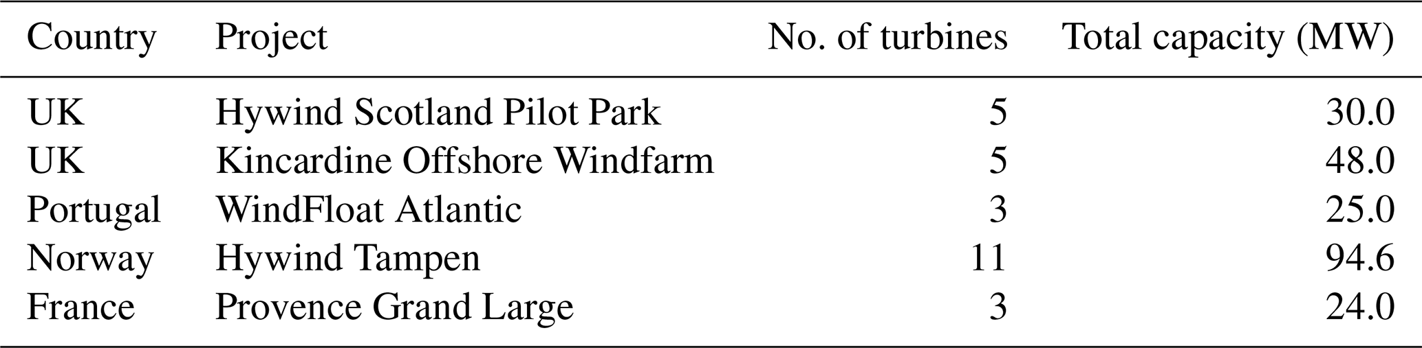
Despite these prospects, the actual development of FOW has been challenging. Since the commissioning of the world’s first FOW farm, Hywind Scotland (Equinor, 2025), in 2017, only a few small-scale FOW projects have been installed globally, totaling around 250 MW, with the major ones shown in Table 1. The primary limitation of FOW development is its high levelized cost of electricity (LCoE), which is estimated to range between EUR 100–200 MWh⁻¹ (Benabadji et al., 2025; Lerch et al., 2018; Stehly et al., 2024; Frazer-Nash, 2023; Shelley et al., 2018), roughly doubled from the recent benchmarked fixed-bottom projects (IRENA, 2023). The higher cost is, in general, driven by the expense of specialized floating platforms, mooring systems, and complex maintenance operations in deep water (DNV, 2025).

Table 1 Overview of major global floating offshore wind projects with more than two turbines (Flotation Energy, 2025).

A major contributor to the LCoE of both fixed-bottom and floating offshore wind is the O&M cost, generally accounting for 20 %–35 % of total LCoE (Wiser et al., 2019; Lerch et al., 2018; Stehly et al., 2020; Frazer-Nash, 2023; Shelley et al., 2018; Ramachandran et al., 2022). Specifically, O&M costs encompass the expenses related to operating, monitoring, and maintaining offshore assets (e.g., turbines and balance of plant) throughout a wind farm’s lifetime, including the revenue losses associated with assets' downtime. The associated O&M activities are predominantly performed in a marine environment, where the logistics of dispatching resources to the offshore site are substantially dependent on weather conditions (DNV GL, 2011, 2020). Therefore, developing an effective logistical strategy is essential for reducing O&M costs, as poorly informed decisions can result in missed weather windows, prolonged resource use, and increased downtime-related revenue losses.

1.2 O&M challenges of floating wind

Floating offshore wind faces greater O&M challenges than fixed-bottom wind. Firstly, floating wind farms are typically located further from shore, which increases vessel transit time and reduces accessibility due to harsher metocean conditions (Carbon Trust, 2022). Secondly, the dynamics of floating platforms introduce higher levels of motion, which may accelerate fatigue and increase failure rates of turbine components (Li and Guedes Soares, 2022), driving up the maintenance demand. Thirdly, additional balance-of-plant (BoP) infrastructure must be maintained, including floating foundations (e.g., floaters, mooring lines, anchors) and dynamic inter-array cables, which also increases demand on maintenance (IRENA, 2024).

The fourth and most critical challenge is the major component replacement (MCR), which has been highlighted in several studies (McMorland et al., 2022; Carbon Trust, 2021; RAMBOLL, 2022). MCR involves replacing large turbine components, such as blades, gearboxes, or generators, which requires specialized heavy-lift assets. In fixed-bottom offshore wind, these operations are typically performed using a jack-up vessel (JUV) or a semi-submersible crane vessel (SSCV). Both vessel types are equipped with advanced sea-keeping systems and lifting capacities of several thousand tonnes, enabling stable operations in offshore environments. However, no existing vessel at the moment, to the authors' best knowledge, can perform MCR directly on floating wind turbines, where a turbine would be in larger relative motion with the working vessel. Specifically speaking, JUVs are limited to shallow waters, as they cannot jack up in depths greater than 60 m (Ahn et al., 2017). SSCVs, on the other hand, cannot yet achieve the precision of operation required when both the turbine and vessel are subject to large motions.

As a result, the tow-to-port (TTP) is currently the default approach for floating-wind MCR. This process is logistically complex and highly weather-dependent, with the major steps highlighted in several studies (Galle, 2023; Brons-Illing, 2015; Crowle, 2021). For example, the Hywind Scotland project conducted its first MCR via the TTP approach in 2023–2024, requiring five 6 MW turbines to be towed 500 km to the port of Gulen by tugboats. Each replacement took 1–2 months on average, encompassing the activities of tow-out/tow-in, offshore disconnection/reconnection, and quayside repair (Tobaben, 2023, 2024; Watissée et al., 2025). The lengthy downtime illustrates the cost implications of additional marine operations and extended turbine unavailability. Alternative approaches such as tow-to-shore, floating-to-floating, and self-hoisting cranes have been proposed to overcome the limitations of TTP (Bayati and Efthimiou, 2021; Carbon Trust, 2021; RAMBOLL, 2022; Dighe et al., 2024). These options could reduce downtime and associated costs but face significant technological, logistical, and market barriers. For now, TTP remains the only implemented approach, although the optimal future strategy will likely depend on project location, infrastructure availability, and technological readiness.

1.3 Current gap in O&M modeling approaches

Given these challenges, reliable O&M modeling approaches are essential to evaluate the economic implications of different strategies on FOW projects. Such models help quantify how choices like MCR strategies influence OPEX, support design-phase decisions such as the selection of floating foundation types, and assess the impact of broader maintenance scopes. In doing so, O&M modeling provides a critical basis for optimizing an O&M strategy to improve the long-term economic performance of FOW farms.

Numerous O&M models have been developed to capture the complexities of offshore wind operations, and several have been further adapted or applied to assess O&M costs for floating-wind technologies (Kolios, 2018; Seyr and Muskulus, 2019; McMorland et al., 2022). A common challenge these models face is the validation, a process of ensuring that the conceptual model is a faithful representation of reality, which somehow requires critical data (e.g., operational information on failures, repairs, costs) that are not widely accessible to the research community. On the other hand, verification, a process of ensuring that a model has been correctly implemented according to its assumptions, remains feasible and is especially important in this context. Verification of a model with other models that have already undergone validation in related domains is considered to be a way of lowering the uncertainty in the outputs of such a model. While this approach cannot substitute full validation against real-world data, it can help uncover inconsistencies, highlight critical modeling assumptions, and build confidence that different tools are producing reliable and reproducible results. This makes verification a vital step for advancing O&M modeling in the field of FOW.

Several verification studies have attempted to compare offshore wind O&M models by running them under a common reference wind farm and O&M scope, then comparing outputs to identify sources of discrepancies. For example, the study (Dinwoodie et al., 2015) benchmarked four models, including NOWIcob (Sperstad et al., 2017), the University of Stavanger O&M simulation model (Endrerud et al., 2014), the ECUME model (Douard et al., 2012), and Strathclyde University’s OPEX model (Dinwoodie, 2013). They found notable differences in predicted availability and O&M costs, particularly under scenarios with constrained maintenance resources (e.g., limited numbers of vessels or technicians), revealing that resource bottlenecks are treated very differently across models. Another study (Smart et al., 2016) compared the NOWIcob model (Sperstad et al., 2017) with the ECN O&M tool (Rademakers et al., 2008) and found the variation in the calculated O&M performance metrics between these models. Although the differences in modeling assumptions were identified in this study, the discrepancies of the results could hardly be attributed to specific assumptions given that the two models relied on fundamentally different simulation approaches. More recently, the open-source O&M model developed by the National Laboratory of the Rockies (NLR; formerly the National Renewable Energy Laboratory, NREL), WOMBAT (Hammond and Cooperman, 2025), was benchmarked against the existing tools mentioned in the previous two studies. WOMBAT generally predicted higher availability and showed differences in vessel costs (particularly for jack-up and cable-lay vessels) as well as downtime associated with major replacements and balance-of-plant failures. However, this study did not systematically trace the observed differences back to their underlying modeling assumptions.

These verification studies highlight that O&M models differ substantially in their underlying approaches, particularly in the level of detail used to represent offshore wind operations. Broadly, they can be divided into two categories. The first consists of heuristic approaches, which use simplified rules of thumb, approximations, or expert judgment to provide rapid estimates of performance. Such models do not explicitly simulate the behavior of every asset but instead rely on aggregated representations to guide decision-making (Douard et al., 2012; Rademakers et al., 2008; Dinwoodie, 2013). The second category employs more detailed system-level simulations, often combining agent-based and discrete-event methods to capture the behavior of individual turbines, vessels, and technicians, as well as the processes they follow during maintenance activities (Sperstad et al., 2017; Endrerud et al., 2014). While both approaches have their merits, the divergence in modeling granularity creates a key challenge for verification: it is difficult to systematically trace how differences in assumptions and inputs affect model outputs. This gap limits confidence in model predictions and hinders the use of verification as a means to improve O&M modeling practices.

1.4 Objectives of the study

The purpose of this study is to examine how modeling assumptions influence the outcomes of offshore wind O&M simulation tools using a structured verification exercise between an open-source model and a high-fidelity research model as a test case. Although the two models differ in their representation of operational processes, they share comparable input granularity and modeling scope, making them suitable for isolating the effects of specific assumptions. The objectives of this work are to

1. identify and categorize key modeling assumptions that differ between the tools, particularly those related to turbine operational states, repair processes, and weather-driven logistics constraints;

2. quantify the influence of these assumptions on core performance indicators such as downtime, availability, and O&M costs;

3. derive generalizable insights on how assumption choices shape O&M simulation outcomes, thereby improving the transparency, robustness, and reproducibility of logistics modeling practices in the wind community;

4. apply the verified modeling framework to evaluate alternative O&M logistics strategies for floating wind, including service operation vehicle (SOV)-based operations, floating-to-floating major component replacement, and condition-based maintenance.

2 Methodology

The methodology consists of three main stages. First, both O&M simulation tools are configured using a common deep-water floating-wind reference case, ensuring that differences in model outputs can be attributed to modeling assumptions rather than scenario inputs. Second, a structured verification framework is applied to identify and incrementally adjust divergent assumptions and to quantify their influence on predicted downtime, availability, and costs. This approach enables the derivation of modeling insights that extend beyond the two tools examined and are relevant for the broader offshore wind logistics modeling community. Finally, the verified modeling setup is used to evaluate several alternative O&M strategies relevant for floating wind. These analyses illustrate how a transparent and verified modeling foundation can support consistent comparison of emerging operational concepts and their cost implications.

2.1 O&M models

Two O&M models are employed in this study: the open-source WOMBAT model developed by the National Laboratory of the Rockies (NLR; formerly the National Renewable Energy Laboratory, NREL) (Hammond and Cooperman, 2022) and the proprietary UWiSE model developed by the Netherlands Organisation for Applied Scientific Research (TNO) (TNO, 2025). WOMBAT is an openly available decision-support tool designed to evaluate the performance and cost of wind power plants during the O&M phase, facilitating research and trade-off analyses on how operational strategies or technological innovations influence wind farm performance. UWiSE, on the other hand, is a proprietary model developed and applied in collaboration with industry partners, building on decades of offshore wind expertise and earlier Energy Research Centre of the Netherlands (ECN) decision-support tools and encompassing a broader set of offshore logistics scenarios, including installation, O&M, and decommissioning for both offshore wind and offshore floating solar assets (Dighe et al., 2024; Huang et al., 2025; Mancini et al., 2024).

Both WOMBAT and UWiSE adopt an agent-based and discrete-event simulation (DES) approach, which is commonly used in offshore wind O&M simulation. In DES models, system behavior emerges from the interactions of individual agents, including turbines, vessels, and technicians, whose activities are triggered by discrete events such as failures, repair actions, or weather-driven delays. Uncertainty is represented through Monte Carlo sampling of failure processes and environmental conditions. The shared high-level modeling principles adopted in both models are summarized below.

• Stochastic failure modeling. Each wind turbine is decomposed into multiple user-defined subassemblies, where each subassembly is characterized by one or more failure modes. In both WOMBAT and UWiSE, failure occurrence is represented stochastically using Weibull-based reliability formulations parameterized by the mean time before failure (MTBF) and a specified shape factor. Random sampling based on these distributions determines the occurrence of failures during the simulation time frame, capturing the probabilistic nature of component reliability behavior. In the present implementation, a single Weibull distribution is assigned to each subsystem, representing a simplified approximation of component reliability behavior.

• Weather-dependent operational constraints. The impact of weather on O&M logistics is represented by combining historical hourly metocean datasets with user-defined operational limits for each activity, such as vessel transits, technician transfers, and on-site repair operations. These weather-dependent constraints determine the accessibility and workability of maintenance resources, thereby influencing weather-related delays, vessel waiting time, and extended turbine downtime.

• O&M strategy. The simulated O&M strategy is modeled by distinguishing between corrective and scheduled maintenance activities. Corrective maintenance represents the reactive actions triggered by failure events and typically involves fault diagnosis and component repair or replacement. Scheduled maintenance, on the other hand, represents preventive actions following predefined calendar-based intervals and normally involves activities such as seasonal inspections.

• Resource dispatch logic. The dispatch of vessels, technicians, and spare parts is governed by a coordinated logistical framework that captures key constraints such as vessel mobilization and charter periods, technician shift schedules, spare part lead times, and overlapping maintenance demands. When resource constraints occur, such as limited vessel or technician availability during simultaneous maintenance requirements, task allocation is determined based on a user-defined planning priority. In this study, maintenance actions are prioritized from replacement to major or minor repair, while scheduled inspections are assigned the lowest priority and are therefore deferred when resources are limited. Dispatch feasibility is further constrained dynamically by weather conditions that limit vessel accessibility and technician workability across different operational steps. It should be noted that, in practice, maintenance prioritization under contractual conditions, such as time-based availability contracts, may be more flexible and depend on contractual considerations. This aspect is not represented in the present models.

• Turbine operational status. The operational status of each turbine, whether fully operational, derated, or shut down, is dynamically modeled to reflect its real-time energy production capability. In both WOMBAT and UWiSE, turbine status is influenced by multiple factors: (i) failure severity, where major component failures can trigger immediate derating or forced shutdown; (ii) maintenance activities, during which turbines shall always be shut down upon technician arrival for inspection, repair, or replacement tasks; and (iii) electrical dependencies within the wind farm layout, where failures or maintenance activities involving inter-array cables, export cables, or the offshore substation result in production losses from all electrically connected upstream turbines until the functionality is restored.

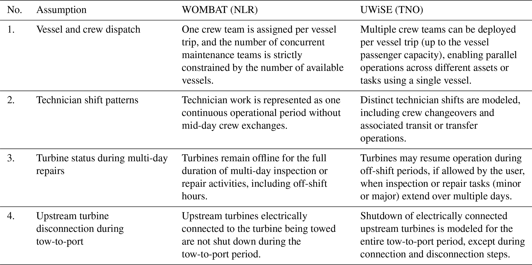
In summary, WOMBAT and UWiSE share a comparable level of modeling granularity and structural logic, providing a strong foundation for model-to-model verification. Nevertheless, they differ in specific implementation assumptions, such as weather dependency, resource dispatch logic, and turbine state transitions, which are expected to influence the predicted outcomes. These key differences are identified in Table 2, serving as the basis for the subsequent verification analysis. Other differences, such as detailed planning logic in the models’ backlogs, are not fully identified and are outside the scope of this study.

Table 2 Summary of key differences in modeling assumptions between WOMBAT and UWiSE.

2.2 Verification process

The verification process, illustrated in Fig. 1, is designed to systematically identify, isolate, and interpret the influence of modeling assumptions on the outputs of discrete-event O&M simulation tools. While WOMBAT and UWiSE serve as the test case in this study, the procedure is general and applicable to other DES-based O&M models.

Figure 1 Overview of the verification process applied to O&M simulation models.

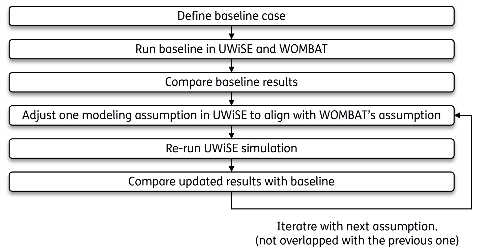
The process begins with the construction of a common baseline scenario, in which both models are configured using the same environmental conditions, turbine characteristics, and maintenance strategies. Each model is then executed under these shared input assumptions. The resulting KPI distributions are compared to assess statistical differences in model responses under nominally equivalent conditions. Next, a series of targeted verification tests is performed through an iterative comparison process. Individual modeling assumptions (listed in Table 2) are sequentially modified within UWiSE to match the corresponding assumptions implemented in WOMBAT while keeping the remaining modeling assumptions unchanged. UWiSE was selected for these adjustments due to its flexible framework, which allows controlled modifications to internal logic and efficient implementation of the investigated assumptions. After each modification step, the resulting KPIs are compared against the common baseline scenario to quantify the influence of that specific modeling difference on downtime, availability, and cost. This process enables isolation of assumption-driven effects on model outcomes. It is noted that a corresponding iterative adjustment process in WOMBAT was not performed within the scope of this study due to time and resource constraints.

Overall, this structured verification framework enhances transparency in model behavior, supports reproducible comparison across tools, and provides generalizable insight into how modeling assumptions shape the results of DES-based offshore wind O&M simulations. Nevertheless, the findings should be interpreted within the scope of the adopted verification approach, where the investigated assumptions were aligned primarily through modifications in UWiSE.

2.3 Inputs

Both models share a comparable input structure. Common input parameters are derived from publicly available and peer-reviewed sources to ensure transparency and reproducibility. The detailed input configurations are presented in Appendix A.

Reference wind farm

The reference floating wind farm used in this study is based on the design framework developed under IEA Wind Task 49 (Hall, 2024), which establishes standardized design bases for floating offshore wind farms across various water depths. The deep-water case (800 m water depth) is selected for model verification. This case represents the Humboldt Wind Energy Area off the coast of California, USA, where site depth ranges between 550 m and 1000 m. The Port of Eureka (Humboldt Bay), located approximately 50 km from the project site, is selected as the maintenance port base. The port is particularly suitable for the tow-to-port maintenance approach due to its deep navigation channel and unobstructed access. The turbine and floating platform designs follow the IEA Wind 15 MW reference turbine (Gaertner, 2020) and the VolturnUS-S semisubmersible platform (Allen, 2020), respectively. The modeled wind farm consists of 67 floating wind turbines, providing a total installed capacity of 1005 MW. The farm layout is adopted directly from the IEA Task 49 design basis (Hall, 2024), as shown in Fig. 2.

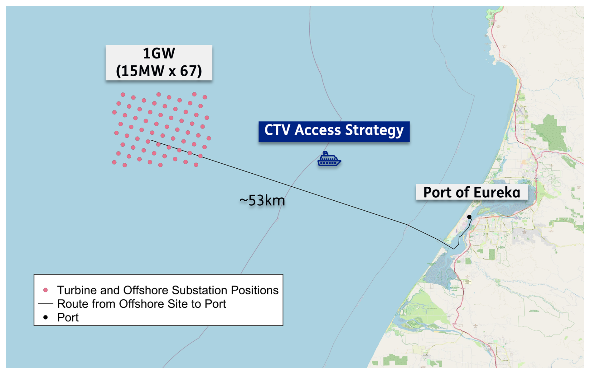
Figure 2 The wind farm layout of reference deep-water floating-wind-farm case. Background map: © OpenStreetMap contributors 2026 (https://www.openstreetmap.org/copyright, last access: 11 February 2026).

To characterize energy production, operational losses, and weather-related accessibility, hindcast hourly metocean data are obtained from the ERA5 reanalysis dataset (C3S, 2023) for the period 1999–2019. The dataset includes key environmental parameters such as wind speed at 10 m height (U₁₀), wind speed at 100 m height (U₁₀₀), and significant wave height (H_s), providing the foundation for simulating both energy generation and marine operational constraints. The metocean data are provided at hourly intervals, where each timestamp represents the environmental conditions during the subsequent 1 h period (e.g., 07:00 represents conditions from 07:00–08:00).

O&M strategy

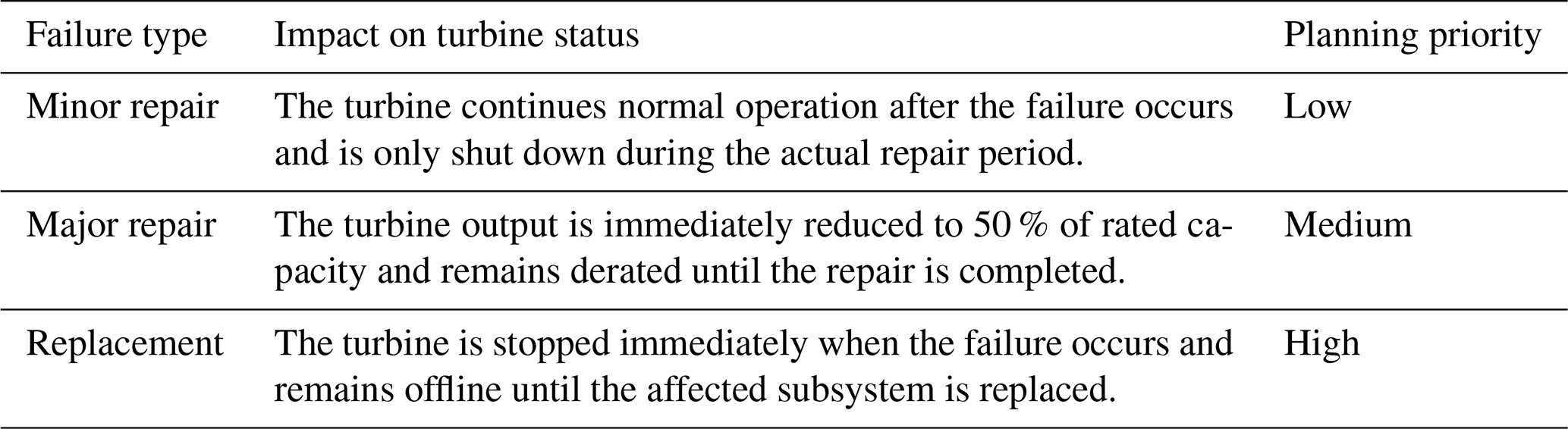
The O&M strategy simulated in both models combines corrective and scheduled maintenance to represent the key operational behaviors and cost drivers of offshore wind farms. An overview of the modeled strategy is shown in Fig. 3. The whole wind farm is divided into several asset groups, including the turbine and the balance-of-plant (BoP) components. Each asset is further decomposed into one or multiple subassemblies, where different failure types defined in Table 3 are assigned to each of the subassemblies. These failures trigger corrective maintenance events. On the other hand, scheduled maintenance activities are performed at fixed calendar-based intervals, representing periodic inspections or preventive tasks carried out during favorable weather periods.

Figure 3 The overview of O&M strategy implemented in both models.

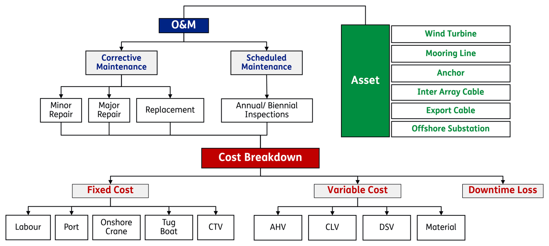
Table 3 Definition of failure types categorized by turbine operational response and maintenance planning priority. The classification follows (Walgern, 2019), with the impact of a major repair adjusted from a 100 % to a 50 % reduction in rated turbine capacity.

Both maintenance categories are represented as sequences of operational steps, including vessel transit, turbine access, and component handling. Each step is assigned specific durations and weather limits (e.g., maximum allowable wave height and wind speed), ensuring that weather-sensitive phases are explicitly modeled. For major component replacement, a tow-to-port (TTP) approach is applied, reflecting the current practice in deep-water floating-wind operations. This process includes critical steps such as mooring line and cable disconnection, towing, and reconnection, all of which require continuous weather windows to ensure feasibility and minimize operational risk.

The resource framework integrates both self-owned and chartered assets. Self-owned resources consist of three crew transfer vessels (CTVs) dedicated to daily operations, two tugboat sets and one onshore heavy-lift crane for TTP activities, and a year-round workforce of 60 technicians working in two alternating 8 h shifts (06:00–14:00 and 14:00–22:00). These resources contribute to the fixed annual maintenance costs, which remain identical across both models. In contrast, specialized vessels such as the cable-laying vessel (CLV), anchor-handling vessel (AHV), and diving support vessel (DSV) are chartered on demand only when failures or inspection campaigns occur. Their costs are determined by the simulated number of mobilizations and charter days. Moreover, downtime-related revenue loss is calculated based on the electricity offtake price, representing lost revenue due to turbine unavailability.

2.4 Evaluation of alternative O&M strategies

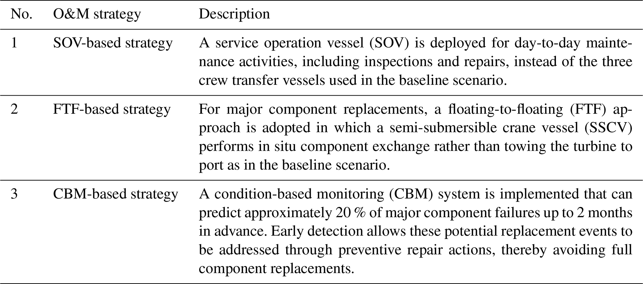
Following the verification exercise, the UWiSE model is further applied to assess the performance of several alternative O&M strategies relative to the baseline scenario. These strategies, summarized in Table 4, represent emerging operational concepts that aim to enhance maintenance efficiency and reduce downtime in floating-wind operations. This analysis illustrates how a verified model can be utilized to quantitatively evaluate the cost-effectiveness and performance implications of innovative O&M approaches, thereby supporting stakeholders in making better-informed strategic decisions.

Table 4 Alternative O&M strategies implemented in UWiSE.

3 Results

3.1 Baseline comparison between WOMBAT and UWiSE

Each baseline simulation was performed with 20 stochastic runs to account for random failure occurrences, and the results presented in this study represent the average values across all runs. A replication analysis was conducted for both models to evaluate the adequacy of the number of stochastic runs, demonstrating that 20 stochastic runs provide sufficiently precise estimates of the reported metrics. Details of the replication analysis are provided in Appendix B. Figure 4 compares the breakdown of annual maintenance cost and annual downtime-related revenue loss (both in the unit of thousands of euros (TEUR) MW⁻¹ yr⁻¹) estimated by WOMBAT and UWiSE. Under the defined input assumptions, approximately 70 % of the total maintenance cost is fixed, reflecting the year-round availability of self-owned resources such as tugboats, heavy-lift onshore cranes, technicians, crew transfer vessels, and the O&M base. These fixed elements are identical in both models. The remaining share is the variable cost, which is driven by model-specific calculations and includes the charter of specialized vessels (AHV, CLV, DSV) and material expenses linked to maintenance events. While both models yield similar total variable cost magnitudes, notable discrepancies are observed in a few cost items. WOMBAT estimates roughly 35 % lower material costs and nearly 500 % higher DSV costs than UWiSE. Moreover, the estimated wind farm downtime, and hence the associated revenue loss, is calculated to be about 200 % higher in WOMBAT than in UWiSE, indicating a significant difference in how operational delays and turbine status are handled between the two models.

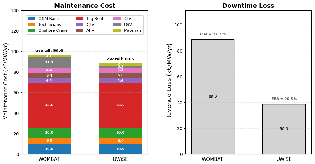
Figure 4 Comparison of maintenance cost, downtime loss, and energy-based availability (EBA) between WOMBAT and UWiSE.

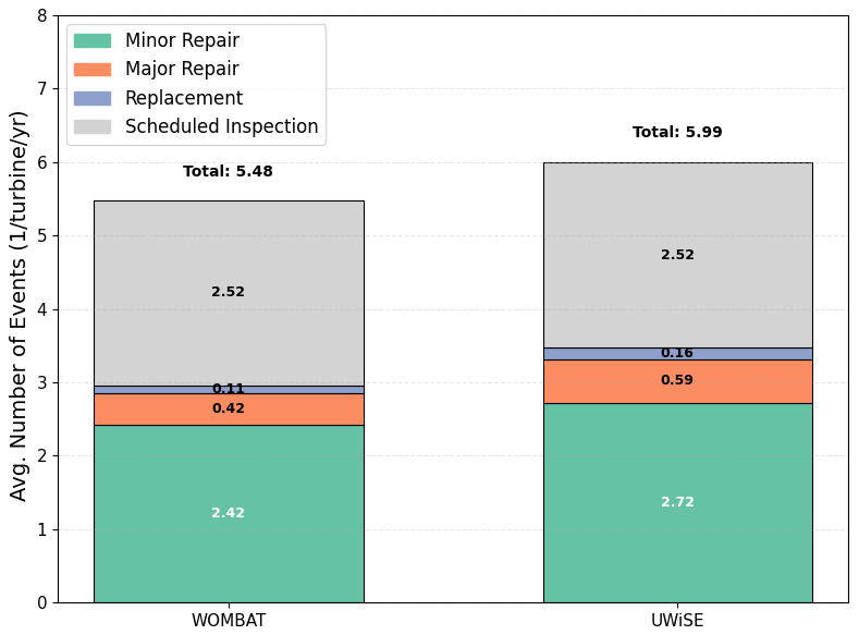
To understand the source of deviation in material cost, Fig. 5 shows the average number of maintenance events per turbine per year. WOMBAT produces about 15 % fewer failure-triggered events (including minor repair, major repair, and replacement) compared with UWiSE. This difference arises from the fact that both models adopt an operation-dependent failure mechanism, where failure likelihood scales with a turbine's accumulated operational time, or uptime, rather than calendar time. As WOMBAT estimates with higher downtime, meaning turbines accumulate fewer operational hours, this eventually results in fewer failures and thus explains the lower material costs observed in this model.

Figure 5 Comparison of average event occurrence between WOMBAT and UWiSE.

The discrepancy in vessel-related costs is further examined in Fig. 6, which normalizes vessel cost, charter days, and mobilization times by the number of corresponding maintenance events. The normalization isolates the effect of differing event frequencies between models, as mentioned previously. In general, WOMBAT shows slightly higher charter days and number of mobilizations per event across all on-demand vessels. This partly results from WOMBAT’s implementation of a minimum charter period for on-demand vessels, which is a parameter requiring a vessel to be booked and paid for at least a number of days regardless of whether the actual operation finishes earlier. Consequently, WOMBAT may overestimate charter days when the operational duration is shorter than the predefined minimum period. This effect, however, has only a minor influence on total cost given the low frequency of AHV and CLV operations. The most substantial difference concerns the estimation of DSVs, where WOMBAT records nearly 10 times more mobilization times per event compared with UWiSE. Specifically speaking, all the DSVs in this case study are used for scheduled inspections (see Appendix A). In UWiSE, two DSVs are mobilized only once per scheduled inspection campaign in that year, while in WOMBAT, DSV mobilization appears to be repeatedly counted within the same campaign period. This modeling difference directly explains the much higher DSV cost in WOMBAT’s results.

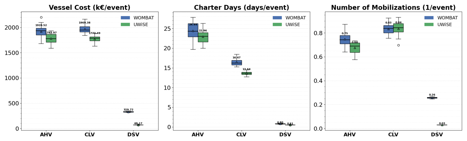
Figure 6 Comparison of cost, charter days, and number of mobilizations for specialized vessels between WOMBAT and UWiSE.

The major discrepancy in the estimation of turbine downtime is explored. Figure 7 presents the monthly time-based availability simulated by both models. This metric differs slightly from energy-based availability shown earlier, as it isolates the effect of mechanical and logistical factors by excluding the influence of wind variability. As such, it provides a clearer basis for comparing the models’ prediction of a wind farm's technical availability performance. Both models exhibit variations around their mean values (shaded area in the figure), reflecting the stochastic nature of failure generation in the simulations.

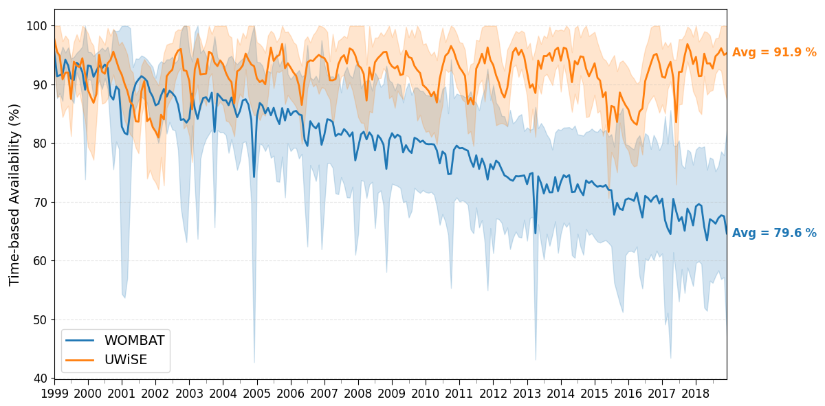
Figure 7 Comparison of average monthly time-based availability between WOMBAT and UWiSE. The shaded area represents ±1 standard deviation across 20 stochastic results.

In UWiSE, time-based availability occasionally drops to around 80 % in certain periods, but it is typically recovered back to a stable range of 90 %–95 % within a few months, indicating an overall equilibrium between failure occurrence and repair capacity. In contrast, WOMBAT shows a gradual and persistent decline in availability over the simulated 20-year period, reaching approximately 60 % by the end of the simulation. This divergent trend in wind farm availability suggests fundamental differences in how the two models handle event backlogs and turbine status responses over time.

Figure 8 Comparison of average monthly cumulative unsolved events between WOMBAT and UWiSE.

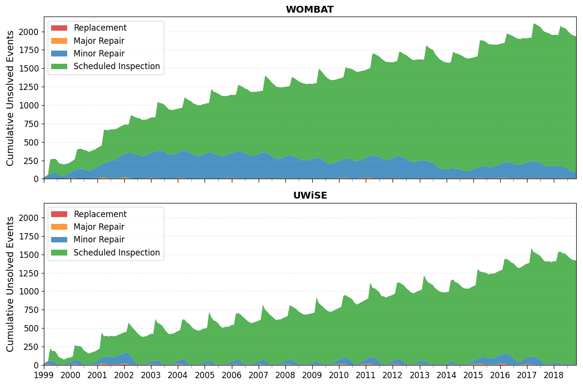
To further explore the causes of these differences, Fig. 8 tracks the cumulative number of unsolved maintenance events, separated by event type, while Fig. 9 summarizes the corresponding event completion rates. The event completion rate is defined as the ratio of completed events to total demand of events generated during the simulation.

Figure 9 Comparison of average event completion rate between WOMBAT and UWiSE.

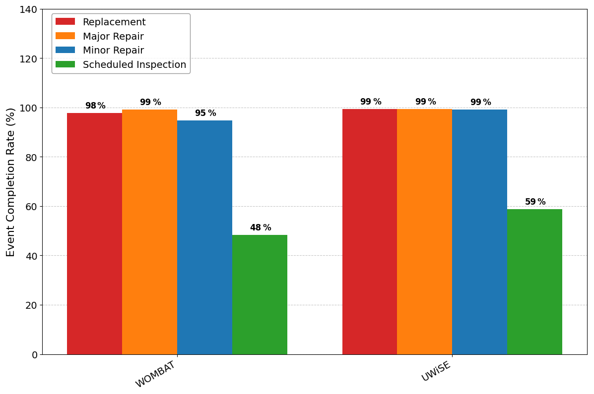
Looking at different event types, the following can be found:

• For major repair and replacement, both models produce highly consistent results. These critical events are almost always resolved within a reasonable time frame, achieving completion rates of 98 %–99 %. This reflects the higher prioritization and effective resource allocation typically assigned to these types of critical failures.

• For minor repair, both models display a clear seasonal pattern. The number of pending events peaks around the winter months, corresponding to the fewer available weather windows in those periods. However, WOMBAT accumulates noticeably more unsolved minor repair events, resulting in an average completion rate of about 95 %, compared to 99 % in UWiSE. This suggests that WOMBAT’s resource allocation or scheduling logic is less efficient in clearing these small-scale but frequent maintenance tasks under the same resource assumptions made in UWiSE.

• For scheduled inspection, both models show that the unsolved events accumulate progressively over time. These events are assigned the lowest planning priority and are often deferred when resources are constrained by corrective maintenance needs. The imbalance between the rate of new inspection needs and the capacity to complete them in time leads to a continuous accumulation of pending events over time. The overall completion rate is only 48 % in WOMBAT and 59 % in UWiSE, indicating that the available fleet and workforce are insufficient to keep up with inspection demands in both models.

To summarize the baseline analysis, both models yield broadly comparable total maintenance cost estimates, with most variations arising from the distribution among specific cost components rather than the overall magnitude. However, a clear divergence is found in downtime estimation, where WOMBAT predicts roughly twice the downtime-related revenue loss compared with UWiSE. This higher downtime aligns with WOMBAT’s lower time-based availability and lower event completion rates, pointing to less effective scheduling and resource utilization within its operational logic. These baseline findings form an essential reference point for the subsequent verification analyses.

3.2 Influence of modeling assumptions on O&M simulation

To evaluate how individual modeling assumptions shape O&M simulation outcomes in DES models, five verification scenarios were implemented in UWiSE, as summarized in Table 5. Scenarios 1 to 4 each isolate a specific modeling assumption related to one of the two aspects shown below. Scenario 5, in contrast, applies all adjustments simultaneously to create a reference case in which the investigated modeling assumptions in UWiSE are aligned with those implemented in WOMBAT. This combined scenario is intended to evaluate the cumulative effect of the investigated assumptions and to assess the extent to which the two models converge when these assumptions are made consistent. The remaining differences between the models under Scenario 5 can therefore be attributed to other unexamined modeling choices or structural differences beyond the scope of this study.

• Scenarios 1 and 2: resource allocation and dispatching logic

• Scenarios 3 and 4: treatment of turbine operational status during maintenance activities

Table 5 Verification scenarios implemented in UWiSE.

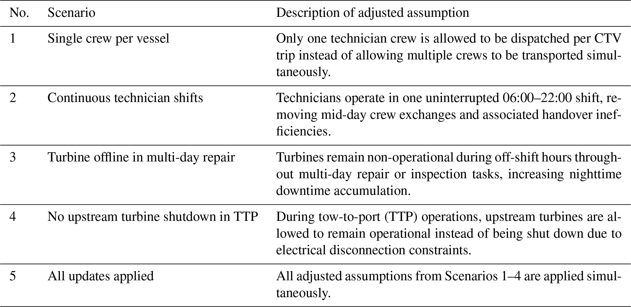
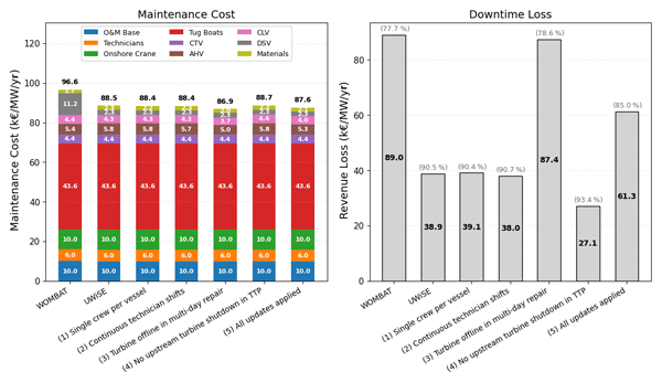
Figure 10 compares the total maintenance costs and downtime-related revenue loss across all scenarios relative to the WOMBAT and UWiSE baseline. Overall, total maintenance costs remain nearly constant, with only minor deviations in variable cost components such as on-demand vessel chartering and material usage. This limited effect is due to the fact that the tested assumptions primarily affect the planning efficiency of frequent, low-cost activities such as minor repairs and inspections, whose associated resources (e.g., CTVs and technicians) are already treated as fixed annual costs in this study. Consequently, the observed variation in maintenance costs is insignificant between verification scenarios.

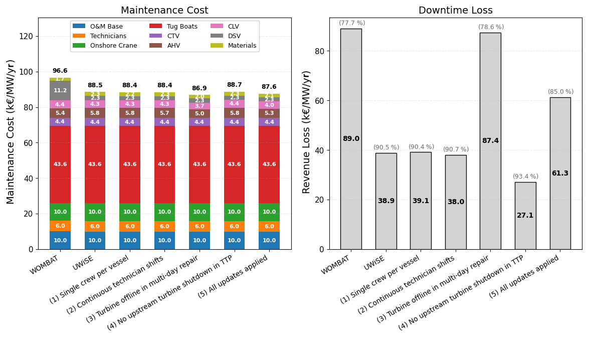
Figure 10 Comparison of maintenance cost, downtime loss, and energy-based availability between WOMBAT and UWiSE scenarios (baseline + 5 scenarios).

Scenarios 1 and 2, which focus on resource dispatching and technician shift patterns, show only marginal influence on downtime loss. In Scenario 1, limiting one crew team to be carried by a CTV slightly increases downtime (< 1 %), while in Scenario 2, assuming continuous technician shifts (06:00–22:00) without handover inefficiencies in between reduces downtime by about 2 %. Since these changes affect only the efficiency of non-critical tasks that do not directly halt turbine operation, their overall impact on downtime remains limited.

Pronounced differences appear in the scenarios where assumptions about turbine operational status during maintenance are altered. In Scenario 3, turbines are modeled to remain offline during off-shift hours (22:00–06:00) when multi-day repair or inspection tasks are ongoing. This assumption nearly doubles the total downtime loss compared with the baseline, as non-operational nighttime hours accumulate substantially over time, particularly during weather-limited seasons. Based on common operational practice, turbines often remain operational during non-working hours for minor, non-critical maintenance. Therefore, WOMBAT’s similar assumption may contribute to a tendency toward higher downtime estimates relative to typical operational behavior. Scenario 4 explores the electrical connectivity of upstream turbines during tow-to-port operations. The total downtime decreases by approximately 30 % when these upstream turbines are allowed to remain operational while the failed turbine is disconnected and towed to port. This scenario underscores the sensitivity of downtime estimates to assumptions about inter-array cable disconnection and power routing. Although technical solutions to maintain upstream production during TTP are being researched, current industry practice still typically requires shutting down upstream turbines during towing for electrical safety reasons (Carbon Trust, 2021).

Scenario 5, which integrates all adjusted assumptions, results in approximately 50 % higher downtime than the UWiSE baseline, bringing its output much closer to the one from WOMBAT. Nonetheless, even after aligning all investigated assumptions, WOMBAT still predicts 30 % higher downtime loss than UWiSE, likely due to deeper differences in resource planning approaches and weather dependency modeling that are beyond the present study’s scope.

Figure 11 shows the average number of maintenance events per turbine per year. As failure generation depends on operational exposure time, scenarios with higher downtime (e.g., Scenarios 1 and 3) produce fewer failures, while those with lower downtime (e.g., Scenarios 2 and 4) exhibit slightly more. These systematic yet minor differences confirm that operational-state assumptions indirectly influence failure occurrence with different calculated turbine uptime.

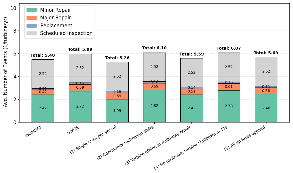
Figure 11 Comparison of average event occurrence between WOMBAT and UWiSE scenarios (baseline + 5 scenarios).

The temporal evolution of time-based availability is shown in Fig. 12 comparing different scenarios. As expected, the trend mirrors the downtime loss results, where scenarios with lower downtime result in higher average availability. Moreover, the figure also reveals that the treatment of turbine operational status significantly affects the dynamics of wind farm availability. Scenario 3 exhibits more pronounced seasonal fluctuations than the baseline, with availability dropping from 90 % to as low as 60 % during harsh-weather periods. In contrast, Scenario 4 maintains more stable availability above 90 % most of the time. Across all UWiSE scenarios, availability eventually recovers a few months after it reaches its local lowest, contrasting with WOMBAT’s continuously declining trend, even when all modeling assumptions are aligned (Scenario 5). This persistent difference likely stems from deeper modeling mechanisms or algorithmic treatments that were not included among the examined assumptions.

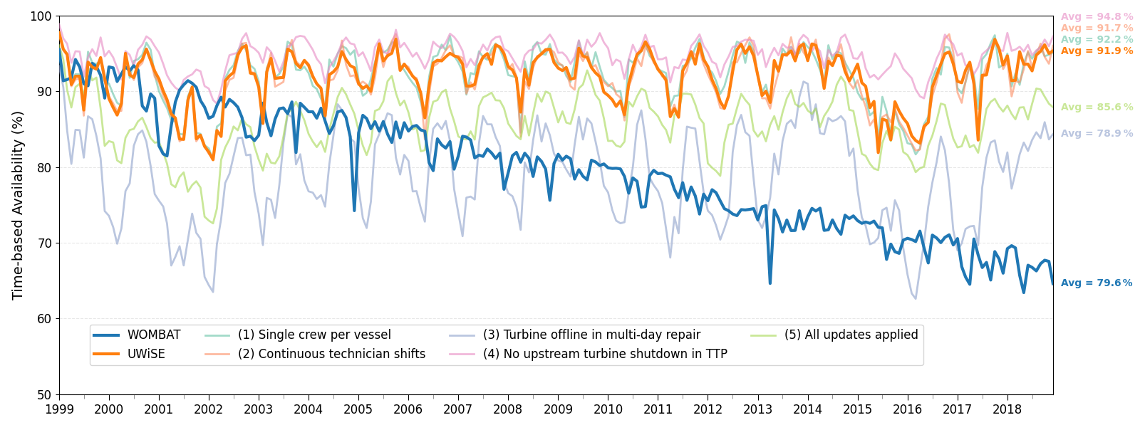
Figure 12 Comparison of average monthly time-based availability between WOMBAT and UWiSE scenarios (baseline + 5 scenarios).

To further assess planning efficiency, Fig. 13 tracks the cumulative number of unsolved maintenance events by type, and Fig, 14 summarizes the event completion rates. These results highlight the effects of resource allocation logic that are not directly visible from the downtime comparisons, as shown earlier. In Scenario 1, the restriction of vessel dispatch efficiency causes an accumulation of minor repair and inspection events, with completion rates dropping from 99 % to 93 % and from 59 % to 20 %, respectively. Conversely, in Scenario 2, which assumes more efficient crew utilization, the inspection completion rate increases from 59 % to 90 %. Although these logistical differences strongly influence task completion dynamics, they do not substantially affect downtime. This is because turbines are assumed to remain operational during the period where non-critical tasks are not fully finished.

Overall, the verification analysis shows that assumptions governing turbine operational states during maintenance are the dominant drivers of downtime and availability estimates in discrete-event O&M simulations. Whether turbines are modeled to remain online during off-shift hours or during tow-to-port operations directly determines the magnitude of production loss. In contrast, logistical assumptions, such as dispatching rules or technician shift structures, have smaller standalone effects but strongly influence maintenance efficiency and can amplify downtime impacts when combined with operational-state assumptions. These findings highlight modeling choices that are widely treated differently across DES O&M tools, underscoring their broader relevance for improving the consistency, transparency, and credibility of logistics simulation models beyond the two examined here.

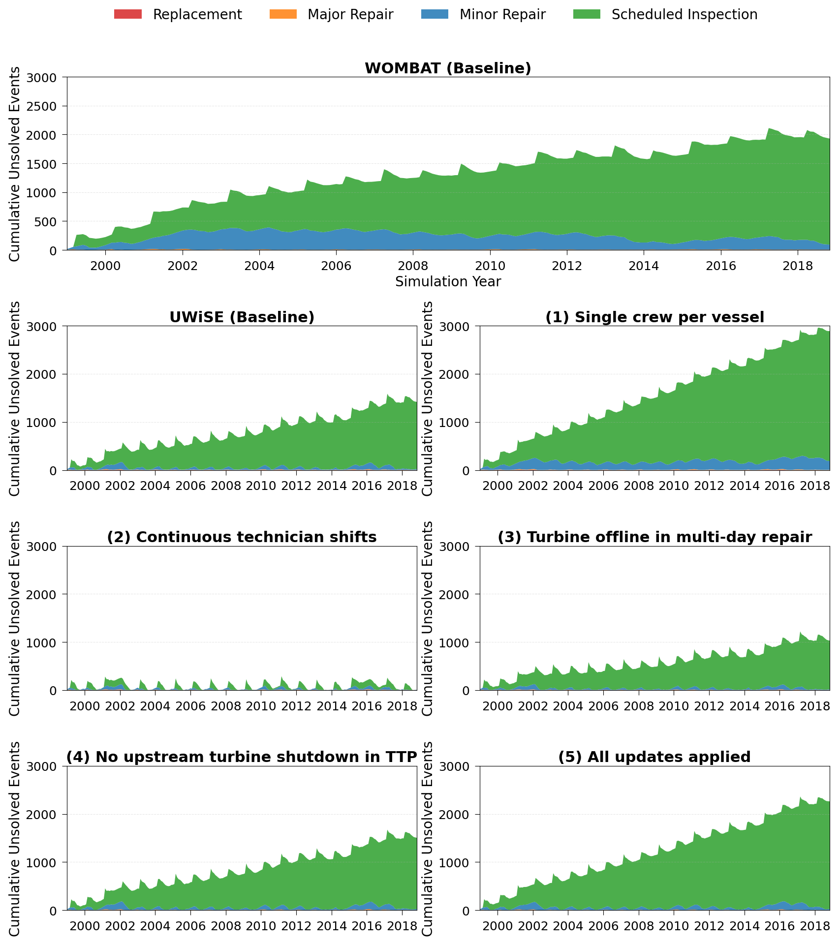
Figure 13 Comparison of average monthly cumulative unsolved events between WOMBAT and UWiSE scenarios (baseline + 5 scenarios).

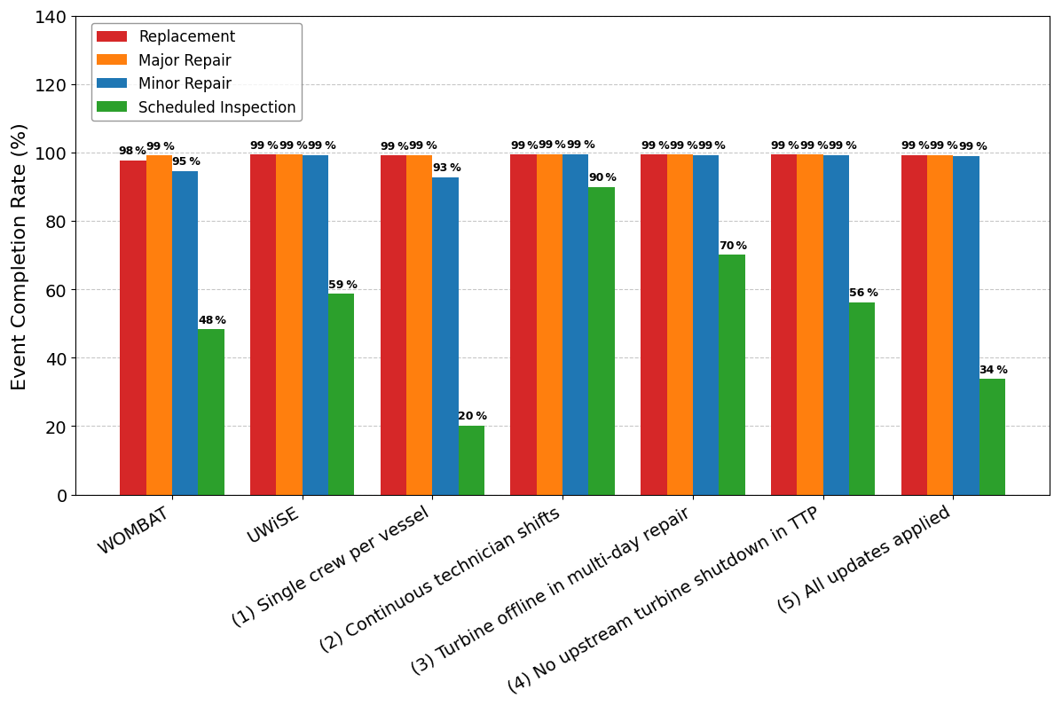
Figure 14 Comparison of average event completion rate between WOMBAT and UWiSE scenarios (baseline + 5 scenarios).

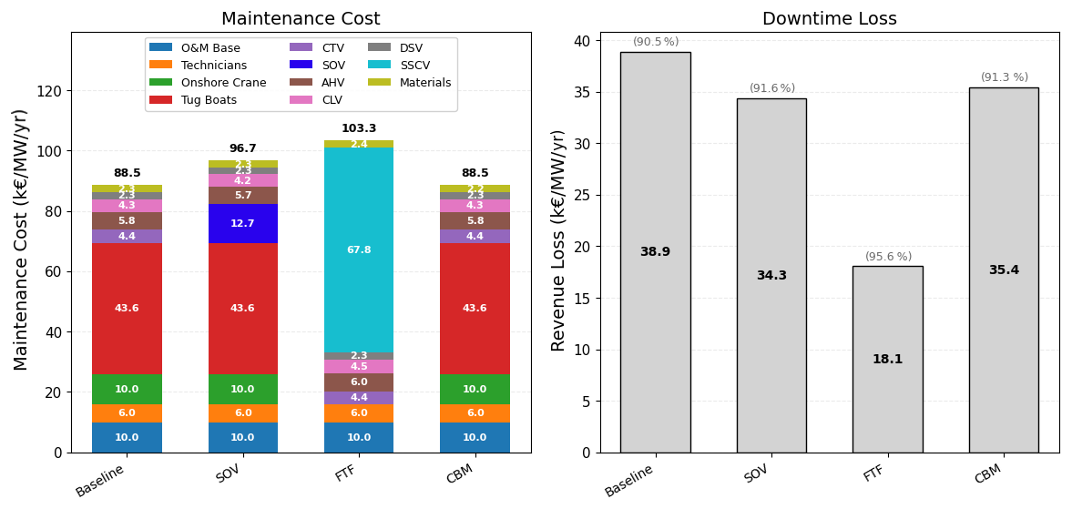
Figure 15 Comparison of maintenance cost, downtime loss, and energy-based availability between baseline and alternative O&M strategies (all run in UWiSE).

3.3 Alternative O&M strategy analysis

Figure 15 presents the comparison of total maintenance costs and downtime-related revenue losses across the tested O&M strategies.

• For the SOV-based strategy, total maintenance costs increase by TEUR 8.2 MW⁻¹ yr⁻¹ compared to the baseline, mainly due to the significantly higher charter rate of a SOV relative to multiple CTVs. On the other hand, the higher maintenance cost is partially offset by a reduction in downtime losses of TEUR 4.6 MW⁻¹ yr⁻¹, as the SOV enables more efficient personnel transfer, longer shift hours, reduced transit time, and greater weather tolerance. As a result, the net overall cost increases by TEUR 3.6 MW⁻¹ yr⁻¹ (3 % higher than the baseline).

• For the FTF-based strategy, total maintenance costs increase by TEUR 14.8 MW⁻¹ yr⁻¹ compared to the baseline, driven by the higher chartering cost of a SSCV. Nevertheless, this increase is fully compensated by a TEUR 20.8 MW⁻¹ yr⁻¹ reduction in downtime losses, leading to the net overall cost reduction of TEUR 6 MW⁻¹ yr⁻¹ (5 % lower from the baseline). The substantial downtime reduction arises from faster on-site component replacements, which eliminate the downtime associated with the lengthy tow-to-port process.

• For the CBM-based strategy, the total maintenance costs remain nearly unchanged, with a slight reduction in material costs of TEUR 0.1 MW⁻¹ yr⁻¹ due to avoided full component replacements. On the other hand, downtime loss decreases by TEUR 3.5 MW⁻¹ yr⁻¹, as early detection through condition-based monitoring allows preventive interventions that reduce the need for prolonged replacement activities. As a result, the net overall cost decreases by TEUR 3.5 MW⁻¹ yr⁻¹ (3 % lower than the baseline). It should be noted that this result assumes the absence of the cost from the CBM system. Therefore, the true economic benefit is likely lower when the cost of implementing CBM is considered.

These downtime dynamics are further illustrated in Fig. 16, which shows the temporal evolution of time-based availability under different strategies. The FTF-based strategy maintains the most stable availability throughout the simulation, consistently staying within the 90 %–95 % range. This result highlights that in situ replacements via an advanced working vessel can effectively mitigate the turbine downtime associated with the current tow-to-port approach.

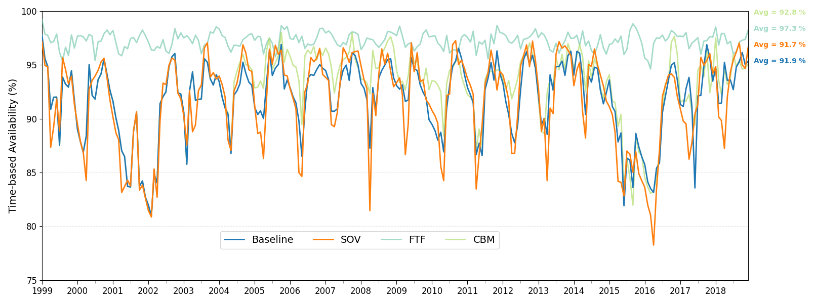
Figure 16 Comparison of average monthly time-based availability between baseline and alternative O&M strategies (all run in UWiSE).

Overall, the results suggest that the FTF-based strategy offers the greatest potential for enhancing wind farm operational performance, reducing overall maintenance cost (including downtime-related revenue losses downtime loss) by around 5 % relative to the baseline scope. Nonetheless, these outcomes are sensitive to key economic and technical inputs that vary across projects, such as cost allocation between fixed and variable cost items, vessel day rates, O&M scope, and electricity price dynamics. Ultimately, the analysis underscores the value of a verified model as a transparent and quantitative framework for systematically evaluating the long-term implications of alternative O&M strategies in floating offshore wind.

4 Conclusions and future work

4.1 Conclusions

This study applied a structured verification framework to examine how modeling assumptions influence the outputs of discrete-event O&M simulation tools for floating offshore wind. Using an open-source model and a high-fidelity research model as a test case, the analysis demonstrated that even under harmonized input conditions, differences in operational logic and process representation can lead to substantial variation in predicted downtime, availability, and cost outcomes. Because these mechanisms are widely shared across DES-based O&M models, the insights gained extend beyond the two tools examined and are relevant to the broader logistics modeling community.

Across all verification scenarios, assumptions governing turbine operational states during maintenance emerged as the dominant drivers of downtime-related production loss. In particular, decisions about whether turbines remain operational during technicians’ off-shift hours or during tow-to-port operations produced the largest changes in downtime and availability. Logistical assumptions, such as dispatching rules and technician shift structures, had smaller standalone effects but strongly influenced task execution efficiency and interacted with operational-state assumptions to amplify overall impacts. These findings highlight modeling choices that are often treated differently across O&M simulation tools and thus represent key targets for improving consistency, transparency, and reproducibility in floating-wind O&M modeling.

The verified modeling framework was then used to evaluate alternative O&M strategies relevant for floating wind. The floating-to-floating major component replacement strategy achieved the greatest performance improvement, reducing total O&M costs by approximately 5 %, while a condition-based maintenance approach reduced costs by around 3 %. These results illustrate the value of combining verified modeling foundations with scenario analysis to assess emerging operational concepts and their cost implications.

Overall, this work delivers three main contributions: (i) a transparent verification approach for diagnosing how modeling assumptions influence DES O&M outcomes, (ii) generalizable insights into the operational-state and logistical mechanisms that shape downtime and availability predictions, and (iii) a demonstration of how verified models can support the evaluation of future O&M strategies for floating offshore wind. Together, these contributions strengthen the credibility, interpretability, and decision-support value of simulation tools used across the offshore wind community.

4.2 Future work

While this study provides valuable insights into the verification and comparative behavior of offshore wind O&M simulation models, several limitations remain and highlight areas for further improvement. These limitations broadly fall into four categories:

• Data-related limitations stem primarily from the absence of publicly available operational data for large-scale floating turbines. The current study relies on maintenance and failure datasets extrapolated from smaller fixed-bottom turbines in the 2–4 MW range. Although scaling relationships are applied to approximate 15 MW turbine behavior, the validity of these adjustments remains uncertain, as larger machines are expected to experience different loading conditions, failure modes, and accessibility constraints. Consequently, both the failure frequency and the associated maintenance cost or duration may diverge from real-world performance. Future work should therefore prioritize empirical data collection from early commercial floating wind farms to enable more accurate calibration and validation of model inputs.

• Model assumption limitations concern several simplifications that, while necessary for comparability, may reduce realism. Both models employ an operation-dependent failure mechanism, where the failure likelihood scales with the turbine's operational time. This approach ensures consistency between the tools but may not fully capture the lifetime degradation patterns observed in practice, which can follow a different trajectory that is more complexly dependent on operational status of a turbine (e.g., a bathtub-shaped reliability curve). Moreover, the representation of tow-to-port operations neglects logistical constraints such as port availability, berth occupancy, and spare part readiness, all of which can substantially affect repair turnaround time and cost. Additionally, human factors, such as technician fatigue, motion sickness, or safety restrictions related to more complex metocean conditions when working on floating platforms, are not yet modeled, though they can significantly influence achievable working hours and resource utilization in offshore environments. These aspects should be incorporated in future model developments to better reflect operational constraints in floating-wind contexts.

• Methodological limitations arise from the scope and resolution of the verification process itself. While this study systematically aligned and tested key modeling assumptions, it did not extend to a detailed, code-level examination of the internal algorithms used by each model. As a result, unexamined differences, such as weather window sampling, resource scheduling heuristics, or task queuing algorithms, may underlie the residual discrepancies observed. Furthermore, the verification relied solely on cross-model comparison rather than validation against real operational data, meaning that both models could still share common deviations from actual performance. Future efforts should therefore move toward code-to-code benchmarking and empirical validation against reference offshore wind farms once such datasets become available. These steps are essential to improve model transparency, credibility, and representativeness of actual operational behavior.

• Financial-scope limitations relate to the simplified economic framing adopted in the analysis. The study intentionally focuses on operational behavior and therefore represents OPEX and revenue losses using simplified assumptions that do not capture project-specific financial structures or offtake arrangements. In practice, differences in O&M strategies influence not only expenditure but also energy revenue profiles, merchant or power purchase agreement (PPA) price exposure, and ultimately the project's cash flow dynamics. Future work could integrate the simulated operational outputs with a more detailed financial assessment model, evaluating metrics such as earnings before interest, taxes, depreciation, and amortization (EBITDA) or cash available for debt service (CADS); incorporating improved price and loss assumptions; and analyzing probabilistic indicators (e.g., P50/P90/P95) at granular time steps aligned with debt-repayment schedules. Such an extension would enable a more holistic evaluation of O&M strategies and generate insights of direct relevance to developers, investors, and lenders.

Addressing these challenges, through improved data acquisition, enriched operational modeling, deeper algorithmic transparency, and integration of more comprehensive financial assessments, will be essential for advancing both the modeling accuracy and the practical decision-making relevance of offshore wind O&M simulation tools. Future work could, for example, leverage operational data from original equipment manufacturers (OEMs) and wind farm operators to validate and refine maintenance and logistics models while incorporating more realistic dispatch strategies, contractual arrangements, and operational decision-making processes.

Appendix A

This appendix summarizes the main input datasets and assumptions configured in both models. The data are drawn primarily from publicly available sources and harmonized to ensure consistency across UWiSE and WOMBAT.

Maintenance data

Table A1 summarizes the failure and corrective maintenance parameters applied to the modeled assets. Turbine-level failure data are primarily based on the large-scale operational datasets reported in Carroll (2016, 2017), which together represent over 350 offshore wind turbines (2–4 MW) of both geared and direct-drive configurations. Each turbine is decomposed into various subassemblies with distinct failure rates, repair durations, and material costs. To align with a larger reference turbine, these data were consolidated by Walgern (2019) into seven representative subassemblies and scaled to a 10 MW class turbine using technology-specific scaling factors. In this study, these parameters are further assumed to be representative of a 15 MW turbine. While this simplification may not fully capture potential reliability improvements or new failure mechanisms expected at larger scales, it provides a reasonable reference in the absence of publicly available field data for this turbine class.

Vessel data

Table A3 provides an overview of the assumed vessel characteristics. Reported vessel parameters in the literature vary widely due to differences in vessel type, design, and project conditions. Therefore, representative values are synthesized from multiple public sources (Brons-Illing, 2015; Dewan and Asgarpour, 2016; RAMBOLL, 2022; Ramachandran et al., 2022; McMorland et al., 2022; Dighe et al., 2024) and based on the authors' expertise. The day rates reported for these vessels are assumed to include fuel, vessel crew, and specialized technicians (e.g., divers). For specialized vessels, a 14 d mobilization period is assumed, encompassing all preparatory steps (e.g., vessel call-off, port readiness, equipment loading, certification, and crew familiarization). Mobilization cost is derived by multiplying this period by the daily rate. Although real mobilization durations are project-specific, this assumption provides a consistent baseline for comparative modeling. Weather limitations of each vessel are represented separately for transit and operational phases. Transit limits define the maximum environmental conditions in which a vessel can safely and efficiently travel from one location to another, whereas operational limits represent the generally more restrictive thresholds governing offshore work (e.g., personnel transfer, cable handling, precision lifting). This distinction allows the models to realistically simulate weather-related delays, where access to the site does not necessarily guarantee workability.

Operational sequences

The stepwise procedures for generic maintenance operations are presented in Table A4. These cover typical inspection, (minor/major) repair, and small-component-replacement workflows, with vessel type and weather limits tailored to the activity. Major component replacement is modeled using the tow-to-port (TTP) approach, with operational steps shown in Table A5, where a defective turbine is disconnected, towed to port, and redeployed after the component is replaced. The slower towing speed and multi-step coordination of this process are explicitly modeled. An alternative floating-to-floating (FTF) replacement concept is also explored in this study, with operational steps shown in Table A6. This approach enables offshore exchange between an advanced working vessel (e.g., semi-submersible crane vessel) and a floating offshore wind turbine. Data for both strategies are adopted and simplified based on Dighe et al. (2024).

Fixed cost

Table A7 lists the annual fixed cost assumptions for a 1 GW floating wind farm. In the baseline case, a CTV-based strategy with vessel ownership is assumed, while an alternative SOV-based strategy is also analyzed in this study with its corresponding ownership costs. Fixed costs additionally include essential onshore service assets such as heavy-lift cranes and tugboats, representing recurring ownership and upkeep expenditures. Port infrastructure upgrades are excluded, as these capital investments are typically outside the operational expenditure scope. Insurance premiums are likewise excluded due to their strong dependence on project-specific parameters (e.g., site metocean conditions, location, and technology maturity), which fall beyond the modeling scope. While such costs can be substantial, they are treated as a separate financial consideration rather than an operational cost element in this study.

In addition, the offtake price of electricity is assumed to remain constant at EUR 80 MWh⁻¹ throughout the simulation, serving as the basis for calculating revenue losses associated with turbine downtime.

Table A1 Summary of wind farm asset types, detailing the subassembly breakdown and associated failure types. Each failure type is characterized by its mean time before failure (MTBF), on-turbine maintenance duration, material cost, and the required service vessel type.

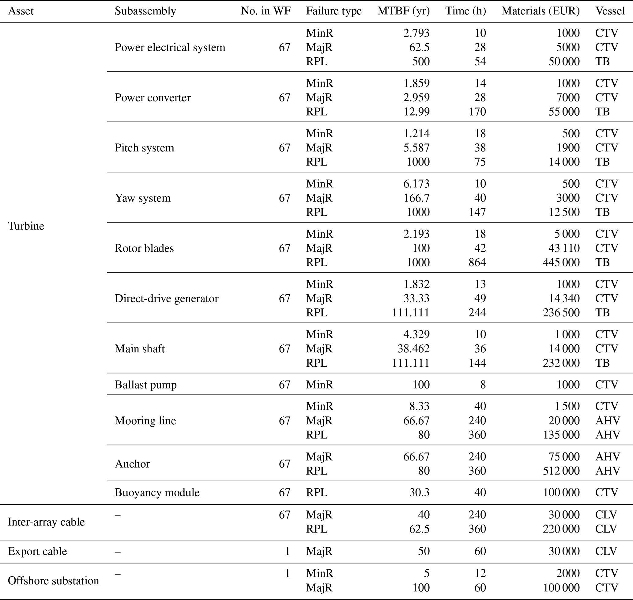
MinR: minor repair; MajR: major repair; RPL: replacement; WF: wind farm; MTBF: mean time before failure. CTV: crew transfer vessel; TB: tug boat; AHV: anchor handling vessel; CLV: cable-lay vessel. Each maintenance task is assigned a crew team of five personnel.

Table A2 Summary of scheduled maintenance campaigns for wind farm assets, including their intervals, on-turbine maintenance time, material costs, and required service vessel types.

¹ CTV: crew transfer vessel; DSV: diving support vessel.
² Each maintenance task is assumed to be carried out by a crew team of five personnel.
³ Each campaign is initiated on 1 April of the corresponding year.

Table A3 Overview of vessel costs, speeds, and operational limits.

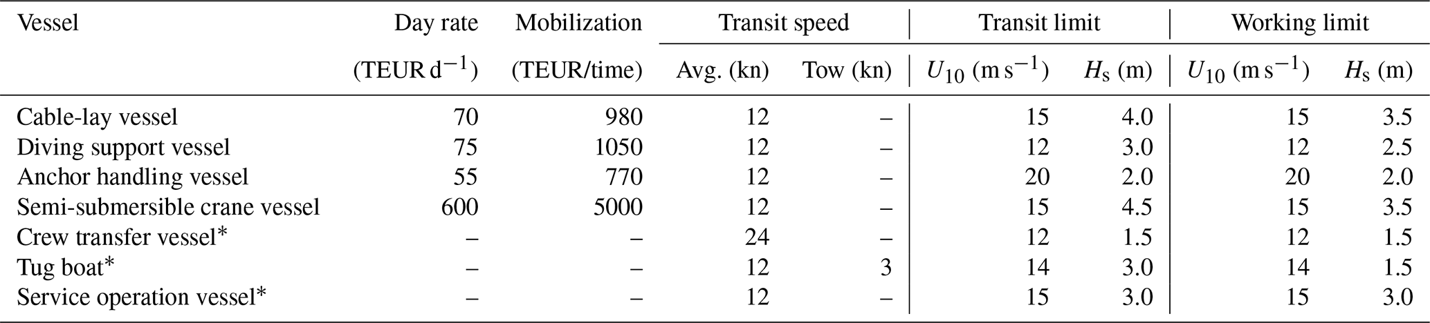
^* Crew transfer vessels, tug boats, and service operation vessels are assumed to be project-owned and treated as fixed project costs.

Table A4 Sequence of actions for generic maintenance (repair, replacement, inspections).

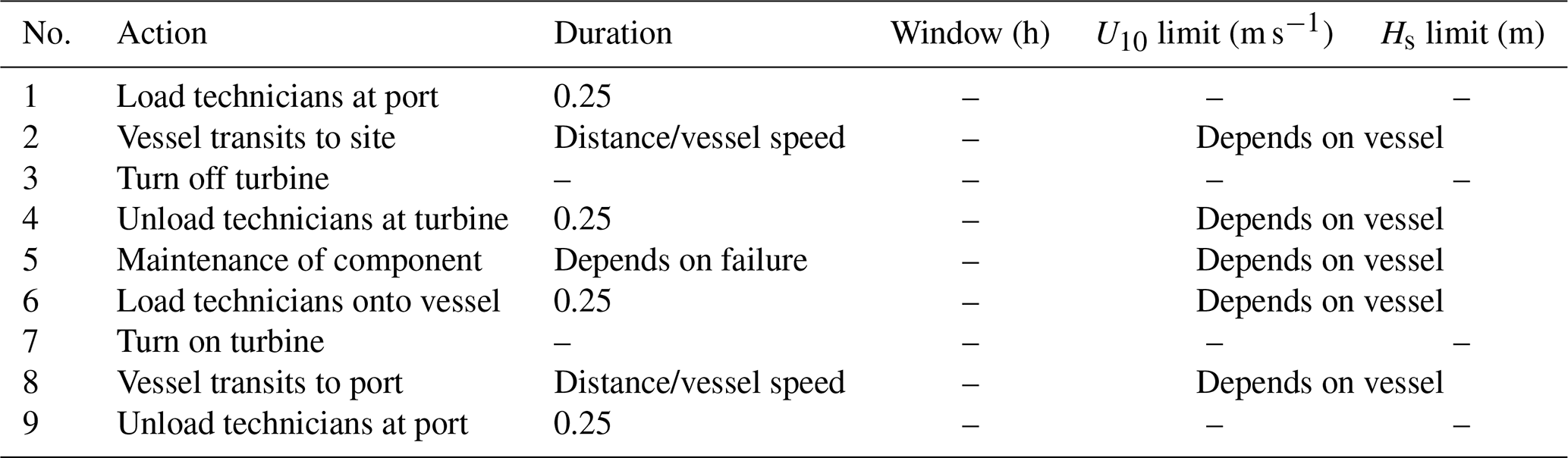
U₁₀ denotes wind speed at 10 m elevation, and H_s is the significant wave height.

Table A5 Sequence of actions for major component replacement based on the tow-to-port approach.

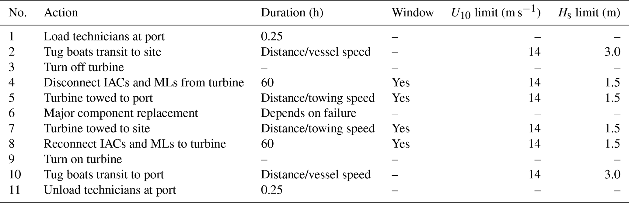
IAC: inter-array cable; ML: mooring line.

Table A6 Sequence of actions for major component replacement based on the floating-to-floating approach.

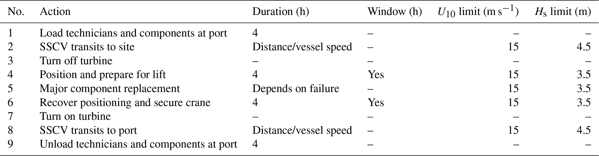
SSCV: semi-submersible crane vessel; IAC: inter-array cable; ML: mooring line.

(Guide to an Offshore Wind Farm, 2025)

Table A7 Fixed cost terms and annual estimates.

Appendix B

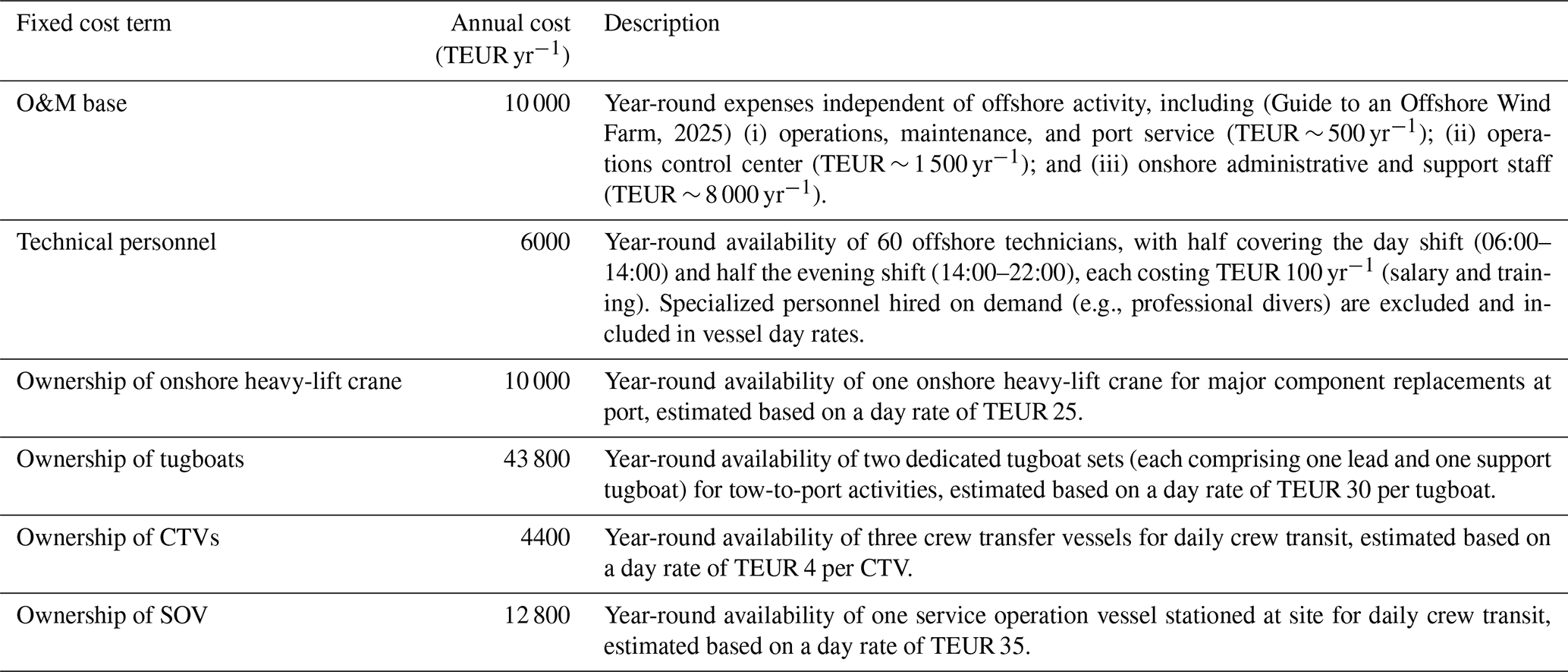
This appendix presents the replication analysis of stochastic simulations, which is performed to evaluate the adequacy of the number of stochastic runs adopted in this study. Since the occurrence of component failures is stochastic, individual simulation runs produce different values for the key performance indicators (KPIs). Consequently, the reported KPIs represent estimates of the expected system performance obtained by averaging multiple independent stochastic runs. The objective of this assessment is therefore to quantify the statistical uncertainty associated with these estimates as a function of the number of stochastic runs.

For a given KPI, the sample mean after n stochastic runs is calculated as

$$\begin{array}{}\text{(B1)}& {\stackrel{\mathrm{‾}}{x}}_n={\displaystyle \frac{\mathrm{1}}{n}}\sum _{i=\mathrm{1}}^n{x}_i,\end{array}$$

where x_i denotes the KPI obtained from the ith stochastic run.

The variability among the stochastic runs is quantified by the sample standard deviation,

$$\begin{array}{}\text{(B2)}& s=\sqrt{{\displaystyle \frac{\mathrm{1}}{n-\mathrm{1}}}\sum _{i=\mathrm{1}}^n{\left(x_i-{\stackrel{\mathrm{‾}}{x}}_n\right)}^{\mathrm{2}}},\end{array}$$

from which the standard error in the sample mean is calculated as

$$\begin{array}{}\text{(B3)}& \mathrm{SE}={\displaystyle \frac{s}{\sqrt{n}}}.\end{array}$$

The standard error represents the uncertainty associated with the estimated mean due to the finite number of stochastic runs. A two-sided 95 % confidence interval of the mean is then calculated as

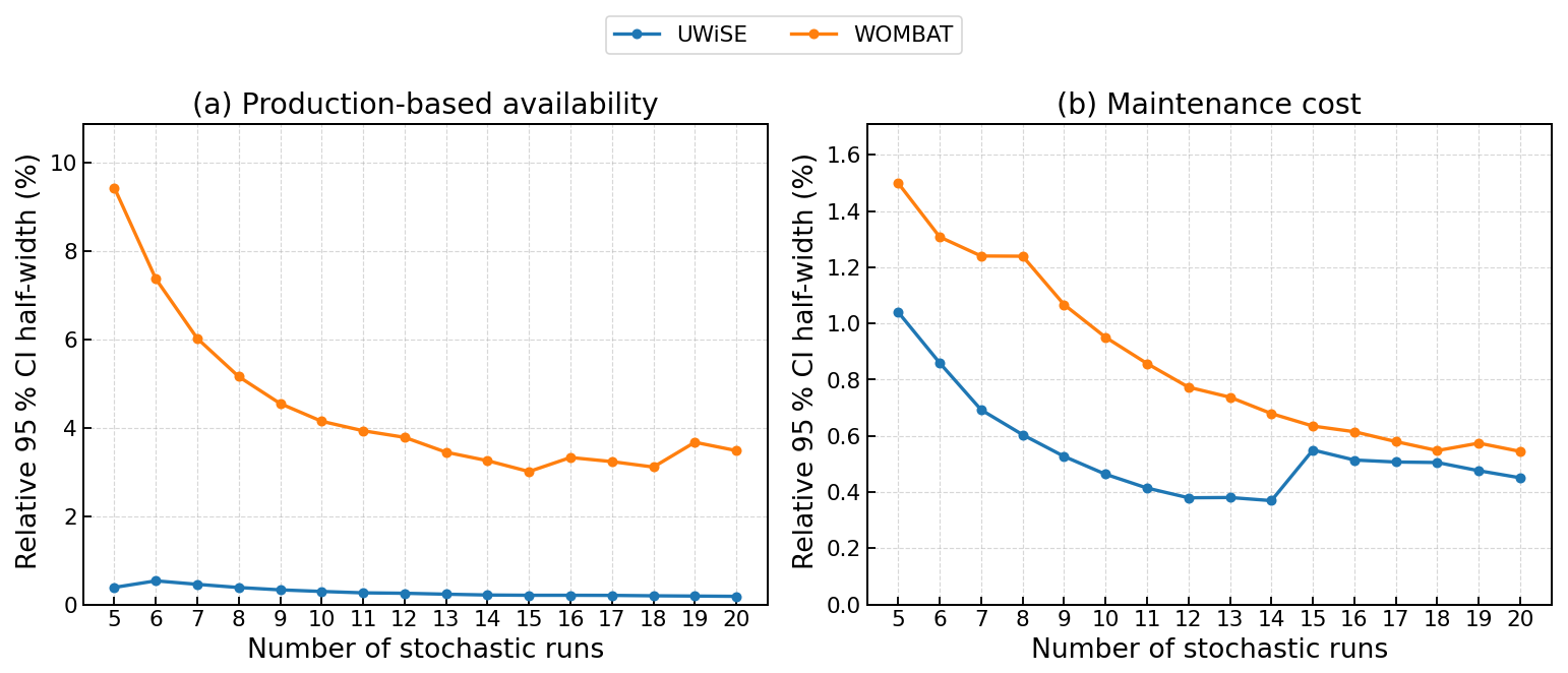
Figure B1 Relative 95 % confidence interval half-width of the estimated mean as a function of the number of stochastic runs for (a) production-based availability and (b) maintenance cost.

$$\begin{array}{}\text{(B4)}& {\stackrel{\mathrm{‾}}{x}}_n\pm t_{\mathrm{crit}}\mathrm{SE},\end{array}$$

where t_crit is the critical value of Student's t distribution corresponding to a two-sided 95 % confidence interval with n−1 degrees of freedom. The value of t_crit depends on the number of stochastic runs and can be obtained from standard Student-t-distribution tables.

To facilitate comparison between different KPIs with different units and magnitudes, the relative confidence interval half-width is calculated as

$$\begin{array}{}\text{(B5)}& {\mathrm{CI}}_{\mathrm{rel}}={\displaystyle \frac{t_{\mathrm{crit}}\mathrm{SE}}{{\stackrel{\mathrm{‾}}{x}}_n}}\times \mathrm{100}\mathit{\%}.\end{array}$$

The relative confidence interval half-width represents the uncertainty in the estimated mean relative to its magnitude. For example, a value of CI_rel=5 % indicates that the estimated mean is associated with a 95 % confidence interval extending approximately ±5 % around the sample mean. Smaller values of CI_rel indicate greater statistical precision and increased confidence in the estimated mean.

Figure B1 presents the relative 95 % confidence interval half-width as a function of the number of stochastic runs for production-based availability and maintenance cost for both UWiSE and WOMBAT, using the same simulation inputs adopted in this study. As the number of stochastic runs increases, the statistical uncertainty decreases, with progressively smaller reductions observed as additional runs are included. This shows that the relative confidence interval half-width falls below around 3 % after around 20 stochastic runs for both models and both KPIs, indicating that the reported average values are estimated with relatively small statistical uncertainty.