Investigating wake reproduction of a model-scale wind turbine: experimental measurements versus large eddy simulation with actuator line

Accurate modeling of wind turbine wakes is essential for understanding turbine performance, wake interactions, and structural loading in wind energy applications. This work presents a combined experimental and numerical investigation addressing key gaps in model-scale wind turbine testing and high-fidelity wake modeling. A major contribution of this study is the design and characterization of a new model-scale wind turbine, TWIST (Turbine for Wind-tunnel Investigation and Scaled Testing), developed to enable high-resolution measurements of near-wake velocity fields and blade deformation. The resulting dataset provides detailed experimental information that remains scarce in the literature, particularly in the near-wake region. In parallel, a continuous actuator line method (cALM) is developed, introducing a novel force-distribution strategy that avoids spanwise averaging along the blade. This approach improves physical consistency and allows for better resolution of loading variations near the blade tip and hub regions. Inflow conditions in the simulations are carefully matched to experimental profiles of mean velocity and turbulence intensity, ensuring that discrepancies primarily reflect modeling assumptions. A systematic comparison between numerical and experimental results is performed to assess the model's ability to reproduce key wake features. Two sensitivity studies are also conducted. First, the influence of blade pitch angle on wake development is evaluated for two operating conditions and compared directly with experimental measurements. Second, blade deformation is analyzed both numerically and experimentally to investigate aeroelastic coupling and its role in observed deviations. Results demonstrate that the cALM captures key near-wake features at 1.41 D, including velocity deficit and wake boundary, and remains consistent with experiments at 4.35 D, with discrepancies mainly near the ground. Overall, the framework improves ALM fidelity and provides a reference dataset for controlled wind turbine testing and wake modeling.

1 Introduction

Accurate modeling of wind turbine wakes is essential for predicting power losses, structural loading, and wake interactions within and between wind farms. These wakes can also affect nearby structures, making reliable wake characterization important for both design and operational decisions. Large eddy simulation (LES) has become a valuable tool for studying these flows, as it resolves the dominant turbulent structures that govern wake evolution and recovery. However, resolving full turbine geometries within LES remains computationally prohibitive, motivating the use of efficient modeling approaches such as the actuator line method (ALM). To ensure predictive capability, ALM-based simulations must be carefully validated against experimental data obtained under controlled conditions. This provides a benchmark for assessing accuracy and guidelines.

The ALM is a widely used tool in the numerical simulation of wind turbines, thanks to its ability to represent a wind turbine without the computational cost of resolving the full blade geometry (Troldborg, 2008). It has become a widely adopted approach in LES frameworks for wind energy research, offering a practical balance between accuracy and efficiency. However, its performance depends strongly on the details of its implementation. Differences in how the ALM is formulated and applied (such as the smoothing kernel or velocity sampling) can lead to significant variations in the simulated turbine behavior and wake characteristics (Jha et al., 2014; Martínez-Tossas et al., 2017). For this reason, careful validation against experimental data remains essential to assess and improve the reliability of ALM-based simulations (Spyropoulos et al., 2021). Several studies have investigated the optimal smoothing length scale for the Gaussian body force distribution used in ALM. Martínez-Tossas et al. (2017) proposed a theoretical framework to determine the optimal kernel width, showing that improper smoothing can lead to over- or under-prediction of aerodynamic forces. Building on this, Martínez-Tossas and Meneveau (2019) introduced a filtered lifting line theory to better understand the impact of force regularization and to improve the physical consistency of ALM implementations. More recent work by Stanly et al. (2022) applied a filtered ALM in LES to better capture wake dynamics and reduce numerical artifacts, while Jha and Schmitz (2017) proposed the actuator curve embedding (ACE) method to improve the representation of blade geometry. Despite these advances, the regions with large radial gradients such as the root and tip of the blades are typically smoothened out by the kernel used in most ALM implementations. Similarly to recent works from Trigaux et al. (2024b, c), we have decided to propose a kernel where the blade tip is not averaged in the radial direction. Additionally in the present implementation, we propose a continuous approach of the ALM (cALM) which improves significantly its computational cost. This method represents forces as polynomials on the spectral element mesh nodes rather than as discrete point sources, constituting a key innovation of this work.

Accurate representation of physical behavior continues to be a key requirement in model development and relies on experimental data. The SWiFT benchmark campaign (Doubrawa et al., 2020) provided valuable field-scale lidar measurements of turbine wakes under varying atmospheric conditions. However, the uncontrolled nature of the inflow affected by shear, veer, turbulence intensity, and thermal stability limits the ability to isolate model performance. A growing body of research has focused on wind tunnel experiments using scaled turbines, where inflow conditions can be precisely controlled (Bastankhah and Porté-Agel, 2017; Han et al., 2022; Hodgson et al., 2023). Small-scale turbines (D≃15cm) have been used to study wake dynamics such as meandering (Coudou et al., 2017), but their low Reynolds numbers introduce scale-dependent effects that distort performance metrics such as the power curve. Larger model-scale experiments, such as the MEXICO project (Schepers et al., 2014; Boorsma and Schepers, 2016), used a 4.5 m rotor to generate high-fidelity validation data, including wake profiles and blade pressure distributions. More recently, Huang et al. (2022) conducted experiments with a 40 cm swept-blade turbine, measuring wake evolution up to 8 D downstream. However, this study used a uniform inflow, which, while useful to isolate blade effects, does not replicate the complexity of an atmospheric boundary layer.

Building on this foundation, this study implements a variant of the actuator line model that introduces targeted modifications to aspects of the conventional approach and evaluates its performance through a direct comparison with wind tunnel measurements. A key feature of this work is the integrated experimental and numerical approach: a custom wind turbine, TWIST (Turbine for Wind-tunnel Investigation and Scaled Testing), was specifically designed, built, and tested under controlled wind tunnel conditions to provide a robust and consistent dataset for validation at 1.41 and 4.35 D downstream. The turbine was operated within a turbulent boundary layer designed to replicate the characteristics of an atmospheric boundary layer on a full scale, ensuring that the experimental conditions are relevant for real-world applications. To enable a meaningful comparison, substantial effort was invested in reproducing the experimental inflow conditions in the LES environment using the open-source spectral element code Nek5000. This included carefully characterizing and replicating the turbulent inflow to ensure that any discrepancies between simulation and experiment can be attributed to the ALM itself rather than differences in the underlying base flow. By closely aligning the experimental and numerical setups, this study provides a robust platform to evaluate the capability of the newly proposed cALM to produce wake dynamics under realistic flow conditions.

The paper is structured as follows.

• –

  Section 2 presents the experimental setup for wind tunnel testing, including a description of the wind tunnel used during the campaign and the instruments used to measure the flow, along with an assessment of their associated uncertainties. This is followed by a detailed description of the TWIST wind turbine model designed for the study.

• –

  In Sect. 3, the numerical setup is introduced, covering the computational code utilized (Nek5000), the mesh generation process, and related simulation parameters.

  • –

    Section 3.2 is dedicated to addressing turbulent inflow generation, with the objective of accurately reproducing the experimental inflow conditions in both mean and fluctuating components.

  • –

    The continuous ALM implemented in the context of this work is then described in Sect. 3.3, also highlighting the differences relative to conventional ALM.

• –

  Section 4 presents a comparative analysis of the experimental and numerical results at two angles of attack. These results are analyzed at two locations downstream of the wind turbine.

• –

  Section 5 compares the results of the blade deformation obtained numerically and experimentally.

• –

  A comprehensive discussion of the results is provided in Sect. 6, evaluating the agreement between experimental and numerical findings and highlighting key insights.

• –

  Finally, the paper concludes with a summary of findings and reflections on the implications of this work.

2 Experimental setup

The wind turbine wake experiment is conducted in the controlled environment of a wind tunnel at the von Karman Institute. By testing in stable flow conditions, the wind tunnel provides an ideal setting to study the performance of the wind turbine under well-defined and repeatable conditions. This controlled setup not only allows for precise testing, but it also facilitates a numerical reproduction of the flow regime. As a result, the discrepancies observed between the experimental and numerical results can be attributed primarily to the modeling of the wind turbine itself, rather than to uncertainties in replicating ambient environmental parameters. This level of control and precision is essential for evaluating the behavior of the ALM used to model the wind turbine in Sect. 3.3.

2.1 L1-B wind tunnel

In order to perform experiments in a controlled environment, we are using the L1B wind tunnel of the von Karman Institute: a low speed, closed-loop wind tunnel with rectangular test section. The flow is driven by a fan with contra-rotating blades, powered by a 580 kW DC motor with variable speed controller. In the center of the test section, the flow velocity can range from 1 to 60 m s⁻¹ in the 1000 hp configuration and from 1 to 22 m s⁻¹ in the 100 hp configuration. A schematic of the facility is provided in Fig. 1.

Figure 1 Top view of the VKI-L1 wind tunnel in wind engineering configuration.

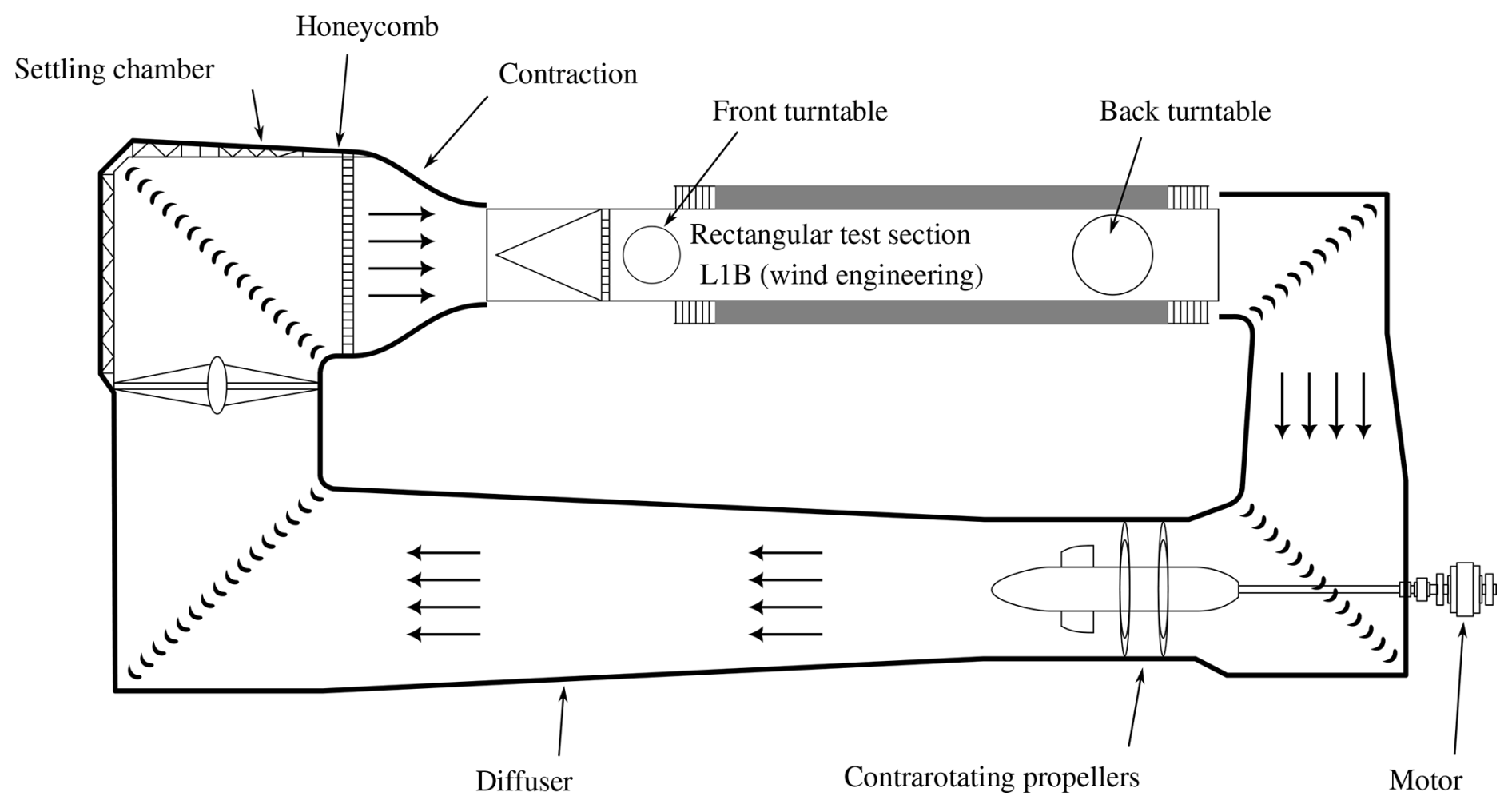
The test section is 2 m high, 3 m wide, and ∼ 20 m long; more detailed dimensions are provided in Fig. 2. This closed test section is used to immerse the experimental wind turbine in a turbulent boundary layer, similarly to the atmospheric boundary layer to which full-scale wind turbines are exposed. An atmospheric turbulent boundary layer is generated in the wind tunnel using a set of roughness elements (Barlas et al., 2015) on the bottom floor, complemented by a grid and fence at the inlet, to create velocity gradients and turbulence. This allows one to reduce the streamwise distance needed to obtain a well-developed velocity profile at the back turntable, where the experiment is performed. A detailed verification of the wind tunnel's suitability for atmospheric flow modeling can be found in Conan (2012). The position of the wind turbine is defined to be sufficiently downstream for a well-developed flow while allowing for enough streamwise distance to measure the wake. In Fig. 1, the wind turbine is positioned at the back turntable, with a more detailed schematic in Fig. 2.

Figure 2 Test section of the L1-B wind tunnel and the three measurement locations.

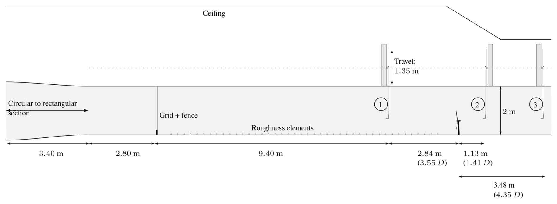
The flow measurements are performed using hot wire anemometry along vertical lines in the test section. Three locations have been used for the measurements, labeled 1, 2, and 3 in Fig. 2. Due to the probe holder's maximum displacement of 1.35 m, the inlet measurement (labeled 1) was performed in two parts to capture the full height. Locations 2 and 3 are limited to the first 1.25 m due to space constraints, yet sufficient to cover the region of interest. All point measurements were sampled at 20 kHz for 5 min each. The uncertainty quantification is described in the following section.

2.1.1 Measurement uncertainties

The uncertainty in the measurements depends on a chain of uncertainties that can be split in two types: the static uncertainty (bias of the calibration) and the random/statistic uncertainty (distribution of the measurement). The static uncertainty, denoted δU, represents the confidence interval attributed to the initial imperfections of the devices used for the calibration. It is computed in the following way:

$$\begin{array}{}\text{(1)}& {\displaystyle }U=\sqrt{{\displaystyle \frac{\mathrm{\Delta }P\cdot \mathrm{298.058}\cdot T}{\mathrm{0.5}\cdot P}}},\text{(2)}& {\displaystyle }\mathit{\delta }U=\sqrt{{\left|{\displaystyle \frac{\partial U}{\partial \mathrm{\Delta }P}}\right|}^{\mathrm{2}}\mathit{\delta }\mathrm{\Delta }{P}^{\mathrm{2}}+{\left|{\displaystyle \frac{\partial U}{\partial P}}\right|}^{\mathrm{2}}\mathit{\delta }{P}^{\mathrm{2}}+{\left|{\displaystyle \frac{\partial U}{\partial T}}\right|}^{\mathrm{2}}\mathit{\delta }{T}^{\mathrm{2}}},\end{array}$$

where U represents the wind speed, ΔP the pressure difference in the manometer, T the temperature, P the atmospheric pressure, and δΔP, δT, δP the respective uncertainty from each measurement device.

Conversely, random uncertainties arise from other factors such as noise and turbulence. Recording for longer time and taking more points for the calibration curves and for the measurements reduces the random uncertainties in the final measurements. The methodology proposed by Vugrin et al. (2007) is applied here to propagate the random uncertainty of a linear fit from each step of the calibrations to the final measurement. With this method, 1 standard deviation of the linear fit is given by the square root of the diagonals of the covariance estimate of the fit. All calibrations in the performed measurement campaigns were linear, except the final hot wire calibration curve, for which the maximum difference in wind speed is taken from the calibration curves of each point. Finally, to ensure a 95 % confidence interval on the measurement, the number of independent samples N is given by

$$\begin{array}{}\text{(3)}& N>{\left({\displaystyle \frac{\mathrm{3.92}}{\mathrm{0.01}}}{\displaystyle \frac{\mathit{\sigma }}{\stackrel{\mathrm{‾}}{U}}}\right)}^{\mathrm{2}}\simeq \mathrm{1.5}\cdot {\mathrm{10}}^{\mathrm{5}}{\left(\mathrm{TI}\right)}^{\mathrm{2}},\end{array}$$

where σ is the standard deviation and $\stackrel{\mathrm{‾}}{U}$ is the mean of the wind speed, which together translate to a turbulence intensity (TI). For a turbulence intensity initially assumed conservatively at 20 %, this leads to 6000 uncorrelated points. The autocorrelation time has been recorded to be between 0.035 and 0.045 s, leading to a minimum sampling time of 3.5 to 4.5 min. Each measurement has therefore been recorded for 5 min per point.

Between 2 and 6 m s⁻¹ (the operating condition range of interest), the static uncertainty ranges from 0.14 to 0.43 m s⁻¹. The random uncertainty from the calibration curves from the pressure manometer and the rotational speed of the wind tunnel rotor together add up to values between 0.20 and 0.24 m s⁻¹ for the same range of velocities. Most of the random uncertainty comes from the calibration curve of the hot wire, which accounts for ∼0.5 m s⁻¹. This uncertainty has been reduced to ∼0.05 m s⁻¹ by repeating the measurement over multiple days. This method was only possible for the calibrations and measurements at locations 1 and 2, which leaves location 3 with higher random uncertainties.

One can argue that, since the static uncertainty was applied to both profiles (with and without wind turbine), this bias would cancel out when examining the relative difference, which then only leaves the random uncertainties. This is the principle applied for the error bars in all the graphs of the present paper.

2.1.2 Quantification of the difference between numerical and experimental results

To evaluate the difference between the numerical and experimental results, we use several well-established error metrics. For all error quantification, the two data sources are resampled at uniformly distributed heights, the zone close to the wall <0.1 m being ignored as it lies outside of the region of interest.

• RMSE (root mean square error) quantifies the average magnitude of the differences between measurements and simulations, with larger discrepancies weighted more heavily.

• MAPE (mean absolute percentage error) expresses the average absolute difference between measurements and simulations as a percentage of the measurements, helping to assess relative accuracy.

• Bias measures the average deviation between simulations and measurements.

• R² (coefficient of determination) is used for assessing the quality of a calibration curve, with values closer to 1 indicating a better quality.

2.2 Model-scale wind turbine TWIST (Turbine for Wind-tunnel Investigation & Scaled Testing)

Previous research (Bastankhah and Porté-Agel, 2017) has shown that scaled-down wind turbines can produce a similar wake as full-scale turbines, given that the main aerodynamic parameters that affect wake behavior remain similar. For this purpose, a few main dimensionless numbers should be matched to ensure that a full-scale wake is reproduced at scale (Schmitz, 2019). First, the tip speed ratio (TSR), that is, the ratio between the incoming flow speed unaffected by the wind turbine and the blade tip speed ($V_{\mathrm{t}}=\mathrm{\Omega }\cdot R$), should be preserved. The TSR determines the advection speed of the vortex generated by the blade tip, thereby triggering turbulent structures in the wake that are key contributors to wake breakdown and recovery. Then, we consider the thrust coefficient (C_t) defined as

$$\begin{array}{}\text{(4)}& C_{\mathrm{t}}={\displaystyle \frac{T}{\frac{\mathrm{1}}{\mathrm{2}}\mathit{\rho }{V}^{\mathrm{2}}A}},\end{array}$$

with T being the thrust force exerted streamwise by the wind turbine and opposing the flow, ρ – the air density, V – the upstream wind velocity, and $A=\mathit{\pi }{D}^{\mathrm{2}}/\mathrm{4}$ – the area swept by the wind turbine. This thrust is responsible for the velocity deficit in the wake.

Finally, the power coefficient (C_p) is defined as

$$\begin{array}{}\text{(5)}& C_{\mathrm{p}}={\displaystyle \frac{P}{\frac{\mathrm{1}}{\mathrm{2}}\mathit{\rho }{V}^{\mathrm{3}}A}},\end{array}$$

with P being the mechanical power extracted from the flow by the wind turbine, as considered at the shaft of the turbine.

Scaled-down experimental wind turbines are typically designed to have a similar TSR and C_t as compared to the full-scale wind turbine, as those parameters are the main factors influencing the resulting wake. At this smaller scale, the wind turbine blades operate at lower Reynolds number (Re), by about 2 orders of magnitude, which impacts the flow behavior locally and the capability to provide lift. Airfoils composing the blade of a model-scale wind turbine must be tailored for low-Re applications. Small-thickness airfoils are selected with a good lift-to-drag ratio and reduced sensitivity to the flow separation at low Reynolds numbers. designed in reality.

In addition, scale model testing introduces a blockage effect due to the closed environment of the wind tunnel. The blockage ratio is defined as the ratio of rotor swept area A, divided by the wind tunnel cross-sectional area. Although it cannot be avoided, it is minimized such that its effect on the flow is reduced. According to McTavish et al. (2013), the blockage ratio should be <10 %, and the minimum distance to a wall should be >1 D. The wind turbine designed in our work has D=0.80 m and a hub height of 0.61 m. According to the above definition, the blockage is thus $\frac{A}{(\mathrm{2}\times \mathrm{3})}\simeq \mathrm{8.4}$ %. A more appropriate blockage concept in the present case consists of ignoring the region below the hub height, because this region is where the ground effect on the wind turbine is intentional. That blockage is obtained as $\frac{A/\mathrm{2}}{(\mathrm{1.39}\times \mathrm{3})}\simeq \mathrm{6.0}$ %. Above the wind turbine, the clearance to the top wall is 1.0 m (or 1.25 D), and it is the closest wall (excluding the ground).

We also wish to produce a wake whose statistics are independent of the Reynolds number, which for turbulence quantities is reached, above $Re\simeq \mathrm{9.3}\times {\mathrm{10}}^{\mathrm{4}}$ as shown in Chamorro et al. (2011) (with Re based on the rotor diameter and free steam velocity). The present wind turbine model operates at $Re\ge \mathrm{35}\times {\mathrm{10}}^{\mathrm{4}}$, which should ensure Reynolds independency of the wake for the mean velocity and second-order statistics.

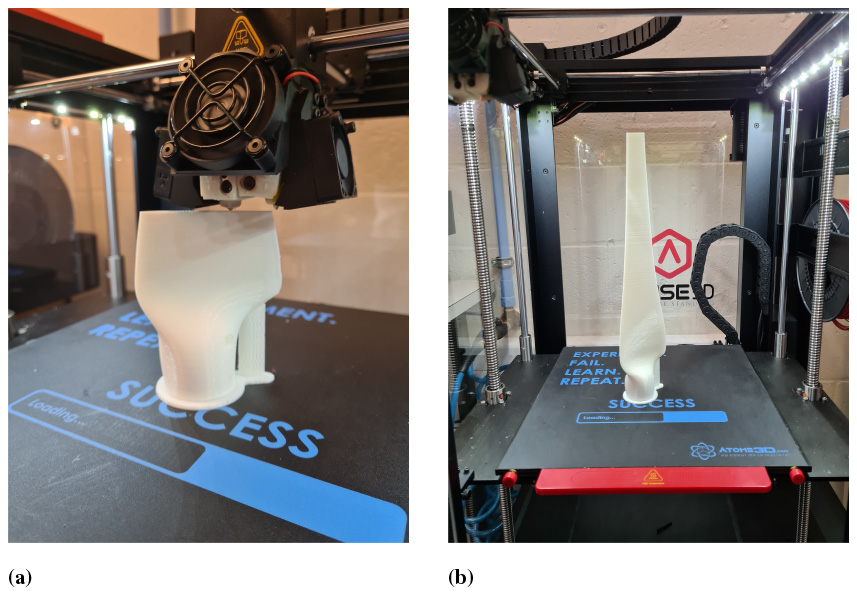
Figure 3 3-D printing process of the blade at UCLouvain. (a) During the printing process, (b) result of the printed blade.

The blades were produced using a 3-D printer of UCLouvain, as illustrated in Fig. 3. The material is a PLA+ plastic, a more ductile variety of PLA. The ductility of the material allows the blade to flex under load without breaking. The airfoil used for the blades is the SD7037-092-88 airfoil, shown in Fig. 4. In the operating conditions used for this experiment, the Reynolds number of the airfoil based on the chord is $\simeq \mathrm{5.0}\times {\mathrm{10}}^{\mathrm{4}}$ throughout the length of the blade.

At the tip of the blade, the Reynolds number is

$$\begin{array}{}\text{(6)}& \begin{array}{rl}& {\mathit{Re}}_c={\displaystyle \frac{Uc}{\mathit{\nu }}}={\displaystyle \frac{\mathrm{29.9}\times \mathrm{0.0259}}{\mathrm{1.54}\times {\mathrm{10}}^{-\mathrm{5}}}}\simeq \mathrm{5.0}\times {\mathrm{10}}^{\mathrm{4}}\text{with}\\ & U=\sqrt{(\mathrm{73.3}\times \mathrm{0.40}{)}^{\mathrm{2}}+{\mathrm{6.0}}^{\mathrm{2}}}\simeq \mathrm{29.9}\mathrm{m}{\mathrm{s}}^{-\mathrm{1}}.\end{array}\end{array}$$

Close to the root of the blade (at 10 % of the radius):

$$\begin{array}{}\text{(7)}& \begin{array}{rl}& {\mathit{Re}}_c={\displaystyle \frac{Uc}{\mathit{\nu }}}={\displaystyle \frac{\mathrm{9.5}\times \mathrm{0.0814}}{\mathrm{1.54}\times {\mathrm{10}}^{-\mathrm{5}}}}\simeq \mathrm{5.0}\times {\mathrm{10}}^{\mathrm{4}}\text{with}\\ & U=\sqrt{(\mathrm{73.3}\times \mathrm{0.10}{)}^{\mathrm{2}}+{\mathrm{6.0}}^{\mathrm{2}}}\simeq \mathrm{9.5}\mathrm{m}{\mathrm{s}}^{-\mathrm{1}}.\end{array}\end{array}$$

At this range of Reynolds number, the flow is in the laminar regime. Consequently, any surface roughness introduced by the 3-D printing process is not expected to significantly affect the flow behavior or promote the onset of transition to turbulence. Therefore, the blades did not go through a surface smoothing process, as this could alter the intended geometry.

Figure 4 Airfoil SD7037-092-88 used for the 3-D printed wind turbine blades.

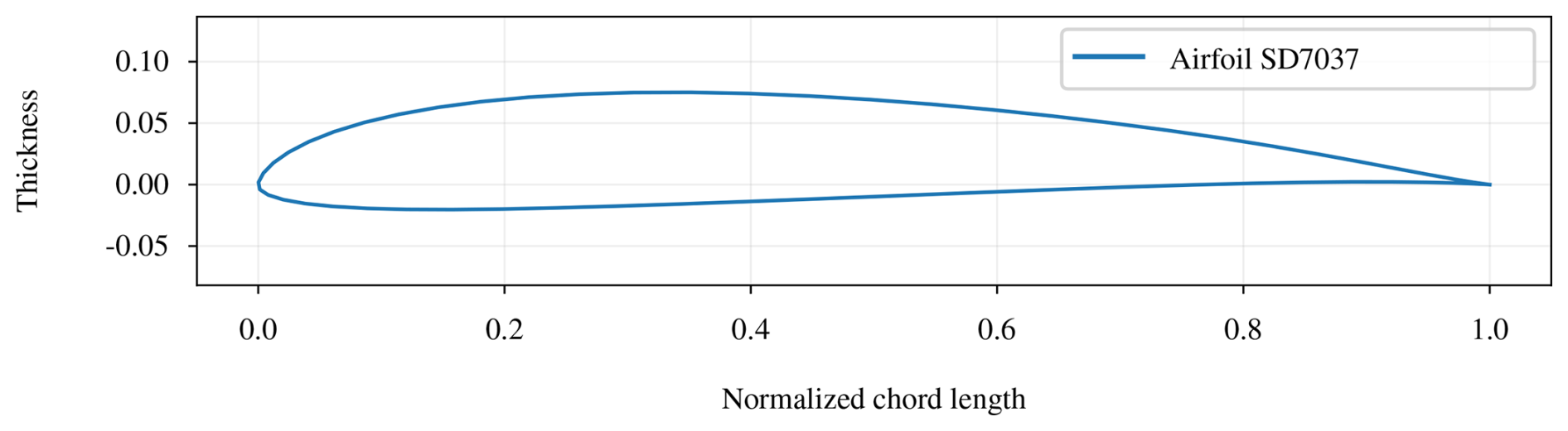
The twist angle and chord distribution of the blades have been designed using a BEM approach using the airfoil SD7037 shown in Fig. 4, and the resulting distribution is provided in Fig. 5.

Figure 5 Blade design parameters for the TWIST wind turbine.

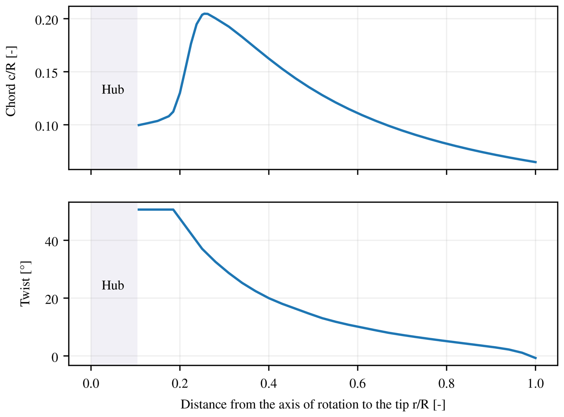
For future projects, a revised blade design could further improve the total power extraction, mostly affecting the aerodynamics in the region close to the blade root, but the current design already serves as a validation case with the main parameters being matched in the ALM model. This design has been simulated using OpenFAST to obtain the C_p and C_t plots shown in Fig. 6, for varying blade pitch angle and TSR, in order to be compared with experimental values.

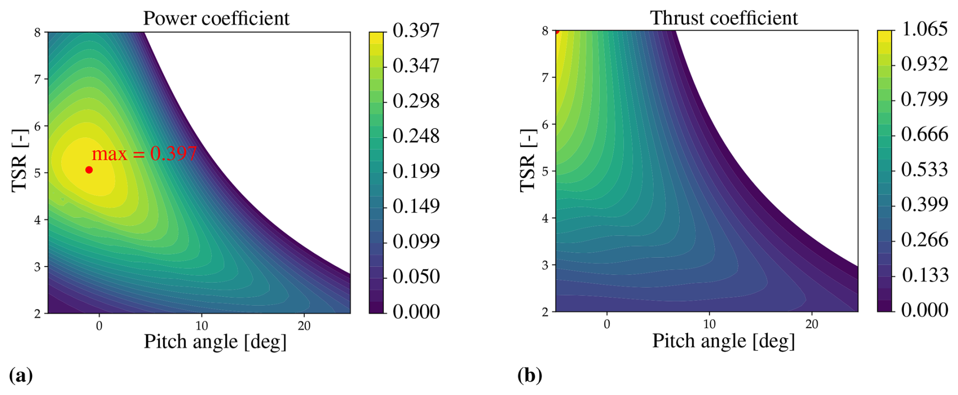
Figure 6 Power and thrust coefficients computed using OpenFAST and the design parameters of the TWIST wind turbine: (a) power coefficient (C_p); (b) thrust coefficient (C_t).

Experimentally, the power curve was derived from electrical power measurements, at a pitch angle of 0°. As anticipated, a discrepancy exists between the measured electrical power and the theoretical aerodynamic power output predicted by OpenFAST. This deviation can be attributed to several sources of mechanical and electrical inefficiency: bearing friction, losses in the bevel gear transmission to the generator, suboptimal generator efficiency (particularly below rated operating speed), and additional losses incurred during AC-to-DC conversion where electrical measurements are acquired. In addition to the mechanical power losses, the numerical simulation may overestimate the power output. This can occur when the lift and drag coefficients are overestimated relative to experimental conditions, which can be affected by the critical number parameter in XFoil.

Figure 7 Experimental power curve of the TWIST wind turbine.

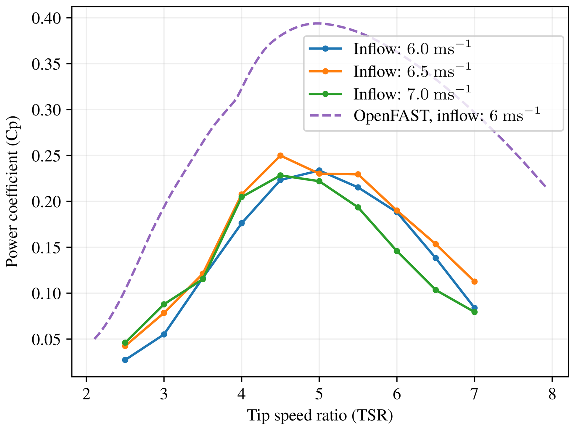
This experimental power curve is compared to the OpenFAST simulations, as shown in Fig. 7. This corresponds to a vertical line in Fig. 6. The experimental measurements have been repeated at various inflow velocities close to the operating conditions of this experiment to assess the sensitivity to the Reynolds number. The results indicate no significant deviation of the curve across different inflow velocities.

Figure 8 TWIST wind turbine model installed in the L1-B test section (a), and its CAD (b).

Figure 9 Mechanism in the nacelle (a), and generator below the wind tunnel floor (b).

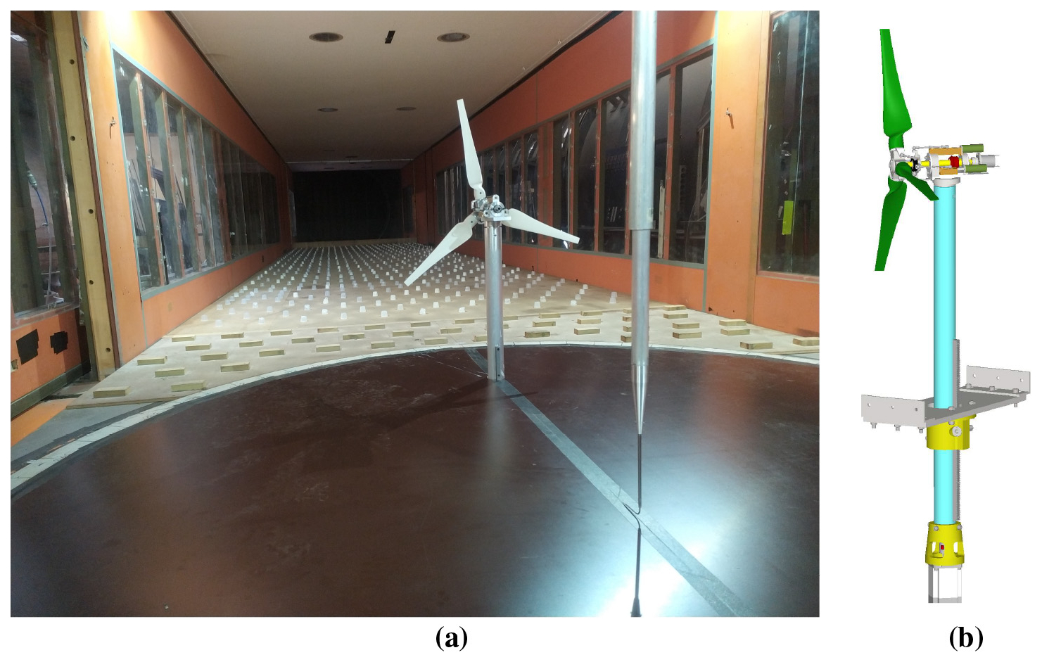
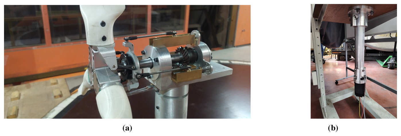
As mentioned before, the turbine model diameter is D=80 cm. The wind turbine support, indicated in Fig. 8, allows for adjusting the yaw and the hub height of the model (set here to 61 cm). In an attempt to maintain a realistic ratio between nacelle size and swept diameter, the generator is placed under the wind tunnel. The power is then transmitted from the horizontal shaft to a vertical shaft through a set of spiral bevel gears, as shown in Fig. 9. Other components are placed within the nacelle, resulting in a diameter of 8 cm, thus 10 % of the swept diameter. The total length of the nacelle, from the base of the blade support to its furthest part downstream, is 23.1 cm, thus approximately 3 times the nacelle diameter. The blades can operate in cyclic and collective pitch control. In the scope of this work, the pitch angle remains constant throughout the experiment.

The aerodynamic power is transferred to the three-phase BLDC generator, to convert to electrical energy. This electrical energy is then rectified to DC using a full bridge rectifier and then used in a series of resistances where the load can be controlled by changing the total resistance. Changing the load is the easiest way to change the reactive torque on the wind turbine and hence control the rotational speed. Twelve resistances are used, each having an ohmic resistance value double of the previous one. This results in a 12 bit binary code for the load of the wind turbine, which provides 4096 possible load values, hence a set of loadings that can be considered continuous. The measurement of power is done on the AC side (before the rectifier to DC) by measuring the voltage and current on one line. In this configuration, the electrical power is measured before the losses in the conversion to DC. The electrical power is computed as 3 times the average power of one line, leading to $P=\frac{\mathrm{3}}{\sqrt{\mathrm{3}}}{V}_{\mathrm{L}}{I}_{\mathrm{L}}$, where V_L is the instantaneous line voltage, and I_L is the instantaneous line current.

In the scope of this study, the TWIST wind turbine is operated at constant rotational speed, as it experiences a steady inflow. The encoder of the generator is used to obtain the rotational speed of the wind turbine during operation, connected to an Arduino microcontroller which also controls the set of relays to act on the resistive load. An integral controller was added to maintain the rotational speed, as it was found to vary otherwise due to changes in resistance caused by temperature fluctuations. Nevertheless, some variability in the rotational speed is still observed, as shown in Fig. 10. Indeed, the controller was tuned to compensate for the heating of the electrical resistances, which is the slowest process, but some fluctuations remain present due to low inertia of the rotor and the flow turbulence.

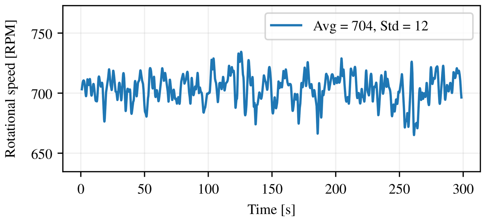
Figure 10 Time series example of the rotational speed of the designed TWIST wind turbine for the present experimental campaign.

3 Numerical setup

In this paper, the code chosen for the LES simulations is Nek5000 (Argonne National Laboratory, 2023), a high-order spectral element code developed by Argonne National Laboratory in the USA. It presents the advantage of being open-source, with excellent scalability for large parallelization, and minimal numerical dispersion and dissipation errors. In addition, its GPU version NekRS would allow our implementations to be ported to this new computational paradigm with relative ease.

The spatial domain is discretized into elements that then use a spectral method to obtain the numerical solution, as described in Patera (1984). This combines the advantages of the spectral method to compute the partial derivatives with high efficiency, together with the local grid refinement of the finite element method. The solution is computed on each element using a high-order weighted residual technique with Gauss–Lobatto–Legendre polynomials (Deville et al., 2002). The order of accuracy of the code is dictated by the order of the polynomials used as a basis function in the discretized elements. The main advantage of a higher-order method is its ability to produce smaller dispersion errors as depicted in Wang et al. (2013), for a similar cost compared to lower-order methods. For a fair comparison with literature, the computational cost of high-order methods is usually expressed in terms of degrees of freedom (DoF), which compares directly to the number of cells of a finite difference solver. In the case of Nek5000, the DoF is calculated by multiplying the number of elements in the computational domain by the number of independent nodes in each element (equivalent to the polynomial order used in each element). Based on previous research using Nek5000 (Fischer, 2013), it is concluded that for most cases the code exhibits optimal performance when using a seventh-order polynomial.

In this code, the subgrid-scale (SGS) turbulence model is closely related to an approximate deconvolution model (ADM). It uses a high-pass filtering procedure to isolate the upper part of the resolved spectral content, which is then employed to estimate the unresolved subgrid-scale contribution. The formulation is primarily controlled by the relaxation (filter-weight) parameter, specified via filterWeight, which governs the level of dissipation and is typically the most influential tuning parameter; a default value of 10 has been shown to provide excellent agreement with DNS at Re_τ≃210 in Schlatter et al. (2004) and is used here. In addition, the filterCutoffRatio (default 0.9) defines the spectral cutoff, effectively using the upper 10 % of the resolved spectrum as an estimator for the subgrid-scale content.

The simulations were performed using a fixed time step of $\mathrm{\Delta }t=\mathrm{2}\times {\mathrm{10}}^{\mathrm{-}\mathrm{4}}$ s, chosen to maintain a sufficiently low CFL number for stable and accurate time integration, while keeping computational cost reasonable. Each case includes an initial spin-up phase to allow the flow to reach a statistically stationary state, followed by an additional relaxation period of 5 times the time constant associated with the exponential moving average used in the control loop, ensuring at least 99.3 % convergence of the controlled turbulence intensity. After this spin-up, statistics were collected over a physical time of 20 s, which was verified to be sufficient for convergence of the resolved turbulent fluctuations in the wake.

3.1 Numerical domain

In order to reproduce blockage effects numerically, the first computational domain corresponds to the wind tunnel test section dimensions, and it includes both the bottom and top walls. It is used to obtain a fully developed turbulent flow with properties similar to those of the experiment. This is achieved by using a recycling method with added forcing, which is described later. To reduce the computational cost, the side walls are not represented, as they are sufficiently far away from the wind turbine not to affect the flow in the mid-vertical plane of interest. Instead, a periodic boundary condition is applied to the sides.

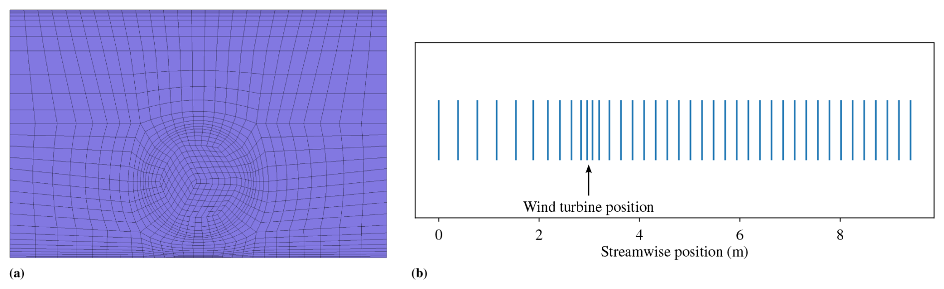
The second domain, which is the main domain, is continuously fed at its inlet using the turbulent flow field sampled at the recycling plane of the first domain simulation. This second domain contains the wind turbine, with blades modeled using an ALM. Both domains have the same cross-section but different lengths, as shown in Fig. 11.

Figure 11 Co-simulation domains with their dimensions and mesh, as used in the Nek5000 setup.

The mesh is refined vertically close to the bottom and top walls to capture the wall-induced shear, and also in the zone of the wind turbine, especially near the tip, as illustrated in Fig. 12. In the cross-section, the mesh is composed of 133 elements in the inner part of the wind turbine region, 360 elements around the tip region, 216 elements close to the bottom wall, 189 elements close to the top wall, and 252 elements in the remaining zones, which totals 1150 elements. The size of each element is constant in the bulk of the rotor swept area, with a refinement applied in the tip region to allow for a sharp transition and to accurately capture the tip vortices. Excluding tip refinement, the mesh can be described as having nine spanwise elements per blade. With a seventh-order polynomial discretization, this corresponds to 63 degrees of freedom, which is directly comparable to 63 cells in a finite difference method. Including the tip refinement increases this number to 77 degrees of freedom. In length, the mesh of the recycling domain is composed of 32 equally spaced elements. The recycling plane is at 5.4 m from the inlet, which is sufficiently far from the outlet to avoid spurious numerical effects. This mesh was created using the GMSH software (Geuzaine and Remacle, 2009).

For the main domain, the length is 9.4 m with 80 elements. The element size streamwise starts identically to that of the recycling domain in the zone upstream of the wind turbine, then becomes finer at the location of the wind turbine, and it is then only slightly coarsened to still properly capture the wake. The wind turbine represented using the ALM is placed at 2.84 m (3.55 D) from the inlet.

Figure 12 Mesh details: cross-section (a) and streamwise refinement (b).

The bottom and top wall of both domains use a shear stress boundary condition, where the value of the shear is obtained from the experimental profile. The value for τ_wall used in the LES simulation was obtained by fitting a log law from the experimental profile. The velocity field at the inlet of the recycling domain is updated at each time step, using a rescaling of the velocity field measured at the recycling plane. Finally, the outlet of both domains is a Neumann open boundary condition with specified pressure.

3.2 Turbulent inflow generation

The co-simulation described in Sect. 3.1 is used to generate an inflow for the main domain, matching as closely as possible that of the experiment, both in terms of mean velocity profile and of turbulence level; more detailed results are presented in Gillyns et al. (2024).

The mean flow is reconstructed using a modified version of the “Recycle and Rescale Method” (R2M) (Xiao et al., 2016), also described in Gillyns et al. (2024). Unlike the original approach, this method does not apply a vertical scaling to match the boundary layer height. Instead, a scaling is performed at every grid point. A moving average of the simulated flow is calculated and divided by the experimental mean velocity profile to generate a spatial scaling factor field. This factor is then applied to the instantaneous flow at the recycling plane before re-introducing it at the inlet. The technique ensures that the inlet profile matches the experimental profile in its time-averaged value, while allowing the turbulence to naturally develop within the recycling region.

However, the turbulence level that naturally develops in the domain remains lower than what is observed experimentally in some regions. This is attributed to upstream elements (grid and fence) that are not reproduced numerically and generate additional turbulence in the experiments. To better match the experimental inflow conditions, a forcing term is introduced in the recycling domain to increase the turbulence level in a controlled manner.

The forcing is constructed as a superposition of sine waves with a wavelength on the order of the integral length scale of the flow. These waves are defined with spatial dependence in the three directions (x, y, and z). In each direction, a set of 10 sine components is used, with a slightly randomized wavelength around the base wavelength, resulting in a total of 30 closely spaced but distinct frequencies. This approach distributes the injected energy over a finite spectral band, avoiding artificial concentration at discrete modes and preventing the appearance of sharp spectral peaks that would require a longer domain to dissipate. This design injects energy primarily at large scales, which then naturally redistributes across the spectrum through the turbulent cascade. In addition, the phases of the sine waves evolve in time, promoting mixing and decorrelation of the perturbation. As a result, by the time the flow is recycled back, the forcing exhibits a more randomized behavior. Spectral analysis at the recycling location confirms that the initially imposed discrete contributions are no longer identifiable and are fully blended into the broadband turbulent spectrum.

Finally, the forcing introduces only a limited quantity of additional energy relative to the already developed turbulence in the flow. This ensures that it acts as a mild correction to the inflow conditions rather than imposing a dominant artificial structure. The amplitude of the forcing is controlled using an integral controller at every grid cell, with the control strategy illustrated in Fig. 13.

Figure 13 Control strategy for the forces in the recycling domain.

A smoothing function is used to remove the forcing near the inlet and the recycling plane, also for numerical stability. The main advantage of the present method is that it allows one to increase the level of turbulence in needed regions, without having to tweak any parameters, since this action is handled by the controller.

The amplitude of the forcing is illustrated in Fig. 14. In this illustration, it appears that the forces are needed only in the lower region, which is confirmed by the vertical profile in Fig. 15. The use of a smoothing function near the inlet and recycling plane is evident from the amplitudes, which vanish in those regions. Within the recycling region, where the forcing is applied, the amplitude of the forces gradually decreases along the streamwise direction. This trend arises from the controller's local operation at each grid point: in the upstream part, stronger forces are initially required to generate the desired turbulence level; moreover, as the flow propagates downstream, the incoming fluctuations begin to resemble those of the experimental profile, hence reducing the need for additional forcing. An important consequence of this approach is that, by the time the flow reaches the recycling plane, the imposed perturbations have largely dissipated. As a result, their influence on the turbulent spectrum becomes negligible, allowing the flow to naturally exhibit the desired turbulence characteristics downstream without contamination from artificial forcing.

Figure 14 Amplitude of the forces used in the recycling region of the numerical setup.

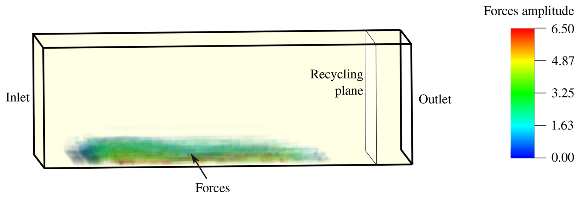
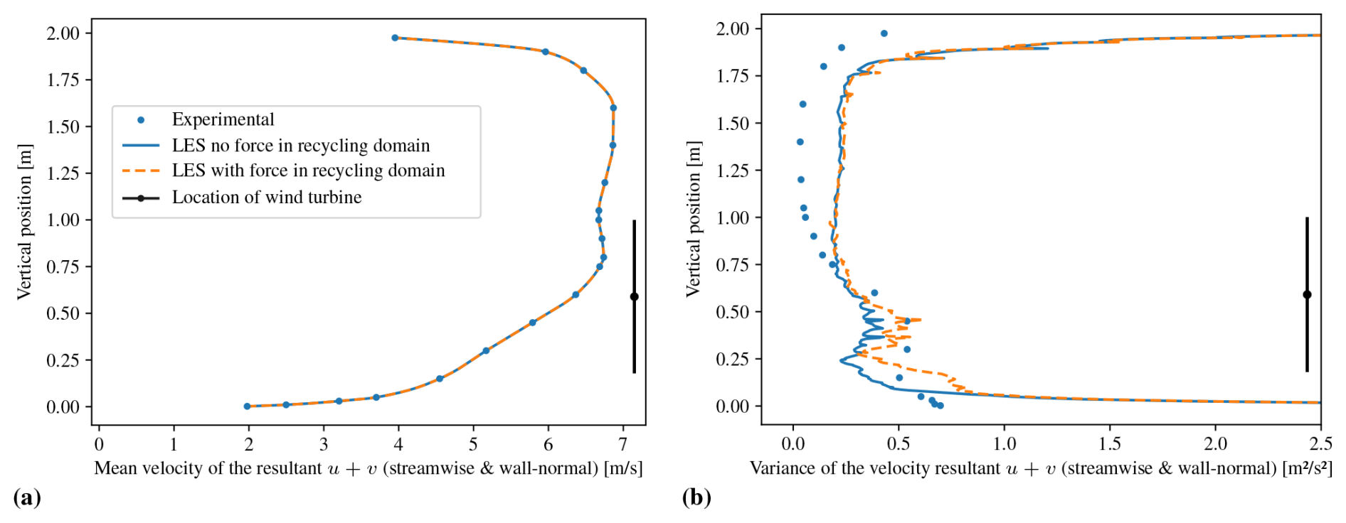
Figure 15 Profile of wind speed at location 1 (inlet of the main domain). Mean velocity (a) and turbulent fluctuation (b).

The resulting mean velocity profile shown in Fig. 15 matches exactly the experimental profile, which is expected since it is imposed in the recycling method. No significant difference is observed in the turbulence fluctuation profile in regions where the experimental turbulence is lower than the numerical prediction (that is, above 0.75 m), which is also as anticipated. Below this height, the turbulence level is increased by the forcing method. To quantify this improvement, the mean absolute percentage error (MAPE) between the experiment and LES in this region was calculated: 31 % without volume forcing, and 16 % with it, representing a 50 % reduction in error.

With the successful alignment of the mean inflow profile and the enhancement of the fluctuating velocity field, the baseline flow now replicates the experimental conditions very closely. This minimization of inflow-induced discrepancies better ensures that remaining differences observed between the experimental and simulation results can be more likely attributed to the modeling approaches, rather than to inflow mismatches.

3.3 Implementation of a continuous ALM (cALM)

The core principle of the ALM is to compute and apply the force induced by the wind turbine on the flow, without explicitly representing it. This method is typically used for the blades. However, in this work we expand the same principle for all three parts of the wind turbine, namely the blades, the nacelle, and the tower.

Both the blades and the tower have a slim aspect ratio, hence it is assumed that using the coefficients of lift (C_l) and drag (C_d) from a 2-D simulation representing the local geometry constitutes a good approximation over most of the span. As for the nacelle, it is assumed to be a bluff body with an associated drag coefficient.

The different steps of the continuous ALM as implemented for the blades are presented hereafter. At each time step and every grid point, the wind speed components are sampled and transformed into a local coordinate system for each blade, as shown in Fig. 16a. This local coordinate system is positioned in the domain at the location of the wind turbine based on the hub height and yaw position. The rotation of the wind turbine blades around the axis of rotation is applied to this coordinate system, which makes it easy to change between using a controller or a fixed rotational speed. In this case, a fixed rotational speed is used.

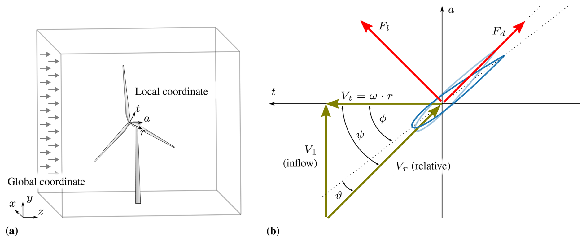
Figure 16 (a) Local and global coordinate systems, and (b) local wind speed and directions around the blade: flow angles, where V₁ is the flow velocity at the wind turbine, normal to the rotor plane, and V_t is the linear velocity of the blade in the rotor plane at the distance r from the center of rotation.

In Fig. 16b, the airfoil composing the blade is shown with a non-zero angle of attack. The forces of lift F_l and drag F_d are, by definition, those aligned with the flow and perpendicular to the flow, respectively. The angle between the effective position of the airfoil and the flow direction is the angle of attack. As shown in the figure, the airfoil is angled in space, labeled ϕ as the sum of the pitch angle and the twist angle (as a function of r). Based on this, the angle of attack labeled ϑ is $\mathit{\vartheta }=\mathit{\psi }-\mathit{\varphi }$.

The forces of lift and drag are obtained using

$$\begin{array}{}\text{(8)}& {\displaystyle }\mathrm{d}L={\displaystyle \frac{\mathrm{1}}{\mathrm{2}}}\cdot \mathit{\rho }\cdot V_{\mathrm{r}}^{\mathrm{2}}\cdot C_{\mathrm{l}}\cdot c\cdot \mathrm{d}r,\text{(9)}& {\displaystyle }\mathrm{d}D={\displaystyle \frac{\mathrm{1}}{\mathrm{2}}}\cdot \mathit{\rho }\cdot V_{\mathrm{r}}^{\mathrm{2}}\cdot C_{\mathrm{d}}\cdot c\cdot \mathrm{d}r,\end{array}$$

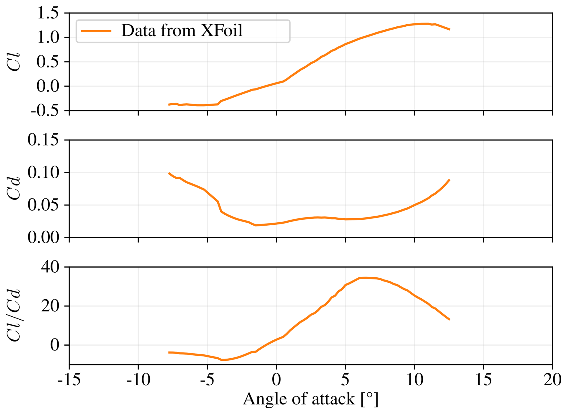
with dL: the discretized fraction of lift force (N); dD: the discretized fraction of drag (N); V_r: the measured relative velocity (m s⁻¹); c: the chord length (m); dr: the discretized fraction of radius (m). The lift and drag coefficients, C_l and C_d, are obtained from the tabulated data using the measured angle of attack and Reynolds number ${\mathit{Re}}_{\mathrm{c}}=V_{\mathrm{r}}c/\mathit{\nu }$. These data were obtained using XFoil at ${\mathit{Re}}_c\simeq \mathrm{5}\times {\mathrm{10}}^{\mathrm{4}}$, N_crit=9, and for the range of angles −7.5 to 12.5°, which is sufficient for the simulation in normal conditions.

The values of lift and drag could be obtained from experimental datasets such as Giguère and Selig (1997); Selig et al. (1995); however in the scope of this work, we used numerical data from XFoil for a generalized approach that can be applied to airfoils for which experimental datasets are not always available at all Reynolds numbers (such as some airfoils used in full-scale wind turbines).

Close to the blade root, there is a transition from the airfoil to an ellipse, and then to a circle. The lift and drag coefficients for the ellipse were computed using OpenFoam, and the drag coefficient for the circle was taken from Munson et al. (2012). It is worth stressing that, in this region, there is a sharp transition in geometry, and the main hypothesis of the ALM to use 2-D polar curves can be questioned. The coefficients used for the lift and drag are shown in Fig. 17.

Figure 17 Coefficients of lift and drag obtained from XFoil for the airfoil SD7037-092-88.

One of the key contributions of this work is the way the wind velocity is sampled and the forces distributed in the grid. The wind speed is sampled at every grid point in the mesh, and the lift and drag are computed at the same grid point, unlike most ALM implementations that consider the center of the actuator line to sample the velocity. This is one of the key differences between cALM and most other implementations, which comes with a scaling computational benefit of removing all the overhead of data transfer in the domain by keeping every node cell independent. We also use a kernel along the actuator line which avoids any smoothing in the radial direction (Trigaux et al., 2024b, c), hence providing a better radial resolution. The Gaussian spreading of the force solely acts in a plane perpendicular to the blade direction. In opposition to standard ALMs, which use a number of actuator points on which a 3-D kernel is applied, this 2-D kernel is applied continuously along the line, using the mesh as a discretization rather than actuator points. The 2-D Gaussian kernel is thus

$$\begin{array}{}\text{(10)}& f_{\left(x,y\right)}={\displaystyle \frac{\mathrm{1}}{\mathrm{2}\mathit{\pi }{\mathit{\sigma }}^{\mathrm{2}}}}{e}^{-\frac{d_{\mathrm{p}}^{\mathrm{2}}}{\mathrm{2}{\mathit{\sigma }}^{\mathrm{2}}}},\end{array}$$

with σ its core size and d_p the distance from the actuator line to the point (x,y) in that plane. The value of σ is chosen as a function of the mesh created for the wind turbine (Jin, 2013; Kleusberg, 2017): $\mathit{\sigma }=\mathrm{2.5}l/n$, where l is the blade length, and n is the number of GLL points along the blade: the number of elements times the degrees of freedom per element (= polynomial order). This guideline applies to a mesh without tip refinement; in this case, the dimensionless value used is $\mathit{\sigma }/l=\mathrm{2.5}/(\mathrm{9}\times \mathrm{7})=\mathrm{0.040}$.

Because a two-dimensional spreading formulation may lead to numerical instabilities at the blade tip when the local mesh is insufficiently refined, an optional tip-spreading correction was implemented. This correction is based on a modified Heaviside function with a smoothing parameter consistent with that used in the two-dimensional Gaussian kernel. In the present simulations, the mesh resolution near the blade tip was sufficiently refined, and the tip spreading was therefore disabled, allowing for a more physically realistic formation and advection of the tip vortex in the wake.

Regarding the velocity sampling method in the cALM, it is evaluated at each nodal point rather than at the center of the line. The sampling velocity used for force computation is therefore obtained independently at every nodal point (i.e., at every degree of freedom within each element). Combined with the continuous kernel representation, this ensures that the computation at each node remains fully independent, significantly improving parallelization and, consequently, computational efficiency.

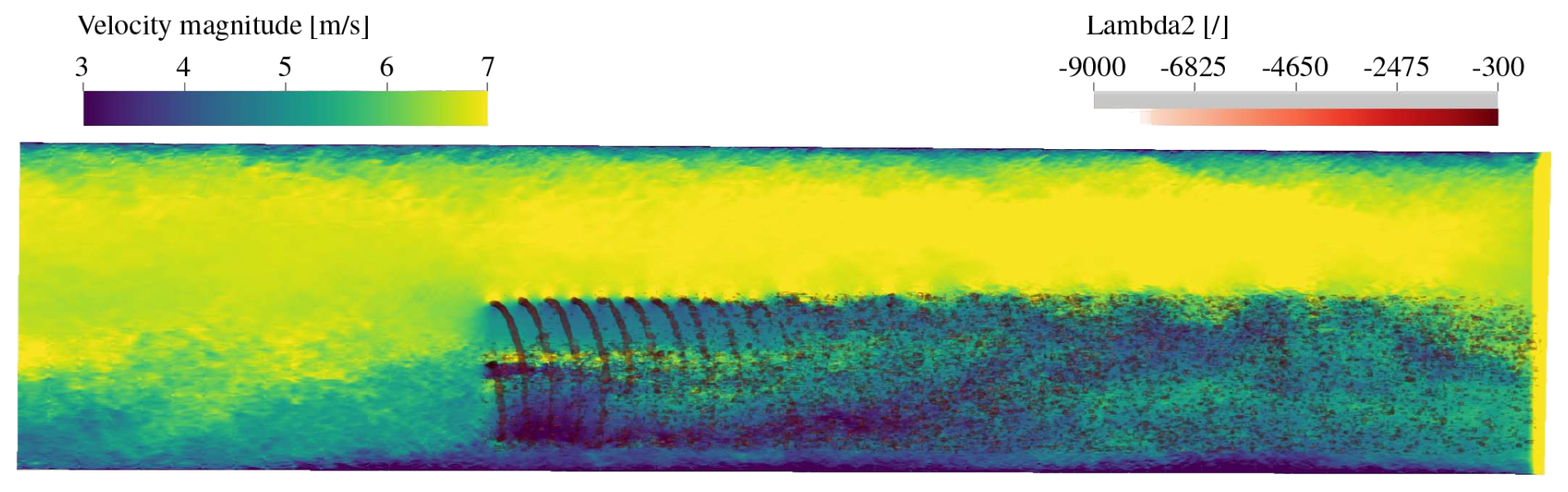
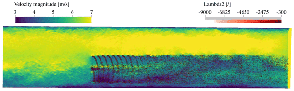
Figure 18 Field of instantaneous velocity magnitude using cALM in the vertical symmetry plane passing through the hub of the wind turbine, on which a lambda2 criterion isocontour is overlaid, highlighting the vortices from the wake.

As a first qualitative view of the resulting flow field, a plot of the velocity magnitude in the vertical symmetry plane is provided in Fig. 18. The differences in boundary layer height between the two walls are clearly visible, due to the increased roughness at the bottom. At the outlet, a flow acceleration that is introduced for numerical stability reasons is also visible, although its effect remains very localized. The tip and root vortices shed by the blades are clearly noticeable. The near-wake is coherent, but it quickly loses its coherence and become fully turbulent, due to the interaction of the tip and root vortices with the tower and the turbulent inflow.

The tower is represented by a non-moving, vertical actuator line at a distance of 13 cm from the center of the blades, which is the distance of the experimental wind turbine design. It is a cylinder of constant diameter (D=60 mm), for which the drag coefficient is taken from the literature (Munson et al., 2012). Its Reynolds number is of the order of 10⁴; therefore the drag coefficient is taken as C_d=1.4.

At the top of the tower, while the actuator line also stops sharply, the numerical effects are not as significant as those at the blade tip because of the much lower relative velocity. Nevertheless, a similar spread as for the tip has been applied for consistency.

The nacelle is a bluff body without longitudinal extent; hence its effect cannot be represented using an actuator line. The drag of the nacelle is computed using the local flow velocity and a drag coefficient, and the resulting force is distributed using a 3-D Gaussian ellipsoid. Its effective frontal area is approximated as a circle with a radius equal to the distance from the turbine center to the blade root $A=\mathit{\pi }\cdot {\mathrm{0.043}}^{\mathrm{2}}=\mathrm{5.8}\cdot {\mathrm{10}}^{-\mathrm{3}}$ m². Determining the drag coefficient of the nacelle is not trivial, as it is not an enclosed body. Therefore, we have adjusted the coefficient empirically until the wake in this region appeared to match observations, resulting in a value of C_d=2. To assess the sensitivity of the results to this modeling choice, an additional simulation was performed with the nacelle drag entirely disabled. In this configuration, the resulting difference remained confined to a narrow vertical band between 0.52 and 0.65 m at location 2 (1.41 D downstream), with differences in streamwise velocity not exceeding 0.15 m s⁻¹. Given the limited spatial extent and small magnitude of this effect, the nacelle drag is not expected to significantly influence the dominant wake features generated by the rotating blades or the principal conclusions of this study.

4 Influence of the blade pitch angle on the wake

In this section, Nek5000 simulations with the cALM implementation are performed at two different pitch angles (+1 and −3°) in order to investigate the influence of this parameter on the resulting wake. These values are selected to represent small physically realistic deviations around the experimental operating condition at 0° pitch. The chosen range is intended to assess the sensitivity of the wake and performance metrics to modest variations in pitch angle that may arise due to controller action, measurement uncertainty, or transient operating conditions.

The parameter that most strongly influences power and thrust, and consequently the wake development, is the angle of attack that each blade section experiences relative to the local flow. As shown previously in Fig. 16b, the angle of attack ϑ depends on both the geometric twist of the blade and the imposed pitch angle, which varies according to controller operation. The twist distribution used in the simulations is identical to that used for manufacturing the 3-D-printed blades, as shown in Fig. 5.

In Fig. 19, the velocity magnitude is extracted along a vertical line at measurement location 2 (see Fig. 2), located 1.13 m (1.41 D) downstream of the wind turbine, for comparison with the hot wire measurements. The dashed lines correspond to the results without the wind turbine, while the solid lines are obtained with it. As indicated in the plot, the experimental results are point-by-point hot wire measurements, and a spline interpolation was used here to connect those values.

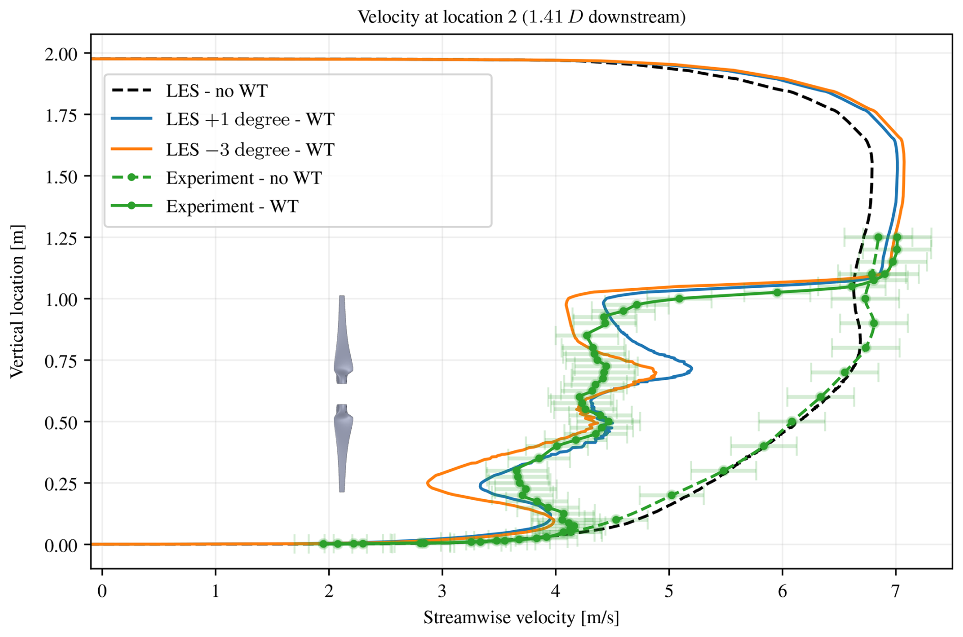
Figure 19 Velocity profile comparing the LES results for two pitch angles with the experimental results at location 2 (1.41 D downstream of the wind turbine). Dashed lines: no wind turbine. Solid lines: with wind turbine. Measurements errors: horizontal bars.

The base flow (without wind turbine) at this location of both simulations show a good agreement with the experiment, with an error in the mean profile characterized by an RMSE of 0.11 m s⁻¹, a bias of −0.0037 m s⁻¹, a MAPE of 1.55 %, and an R² value of 0.98 thanks to our previous effort to match the mean profile and turbulence level of the inlet in Sect. 3.2 and in Gillyns et al. (2024). With this small error in the base flow, it is expected that the observed differences when the wind turbine is present can be attributed to the modeling of the wind turbine itself (i.e., the simplified modeling of the blades and tower effects on the flow using the ALM, and of the nacelle effects) rather than to inaccuracies in the base flow.

We also observe in Fig. 19 that the experiment exhibits an intricate change in the velocity gradient caused by the interaction between the turbine wake and the ABL and that this is fairly well captured by the simulation. The ability of the model to reproduce such detail in regions of high gradient near the tips can be attributed to the present ALM implementation, made more precise by not averaging in the blade direction. We cannot claim that the method is accurate near the blade root as the aerodynamics of the transition from an airfoil to an ellipse and then to a circle cannot be well represented by an ALM. The same comment applies to the nacelle, which is modeled using a drag force spread over an ellipsoid.

The simulation also shows good agreement with the experimental slope in the transition zone between the freestream and the wake, where the tip vortices are most prominent, particularly at a height of 1 m. The accuracy of the ALM in capturing this slope (vertical shear) largely depends on the tip spreading. When the tip spread is minimal (i.e., a sharp tip transition), the ALM represents the blade tip more accurately, resulting in better agreement with the experimental data, as seen in Fig. 19. For the −3° case, simulations with and without tip spreading were compared, revealing a significant difference in the slope (vertical shear) in the transition zone at a height of 1 m. With tip spreading, the vertical shear at that location is 15 s⁻¹, whereas without tip spreading it increases to 47 s⁻¹. By comparison, the experimental profile shows a vertical shear of 34 s⁻¹. However, achieving this level of agreement requires a sufficiently refined mesh near the blade tip. In the velocity deficit induced by the blades, the +1° case appears to agree better near the blade tip, while the −3° case shows better agreement near the blade root. This trend is observed in both the upper region (0.6 to 1 m) and the lower region (0.2 to 0.6 m).

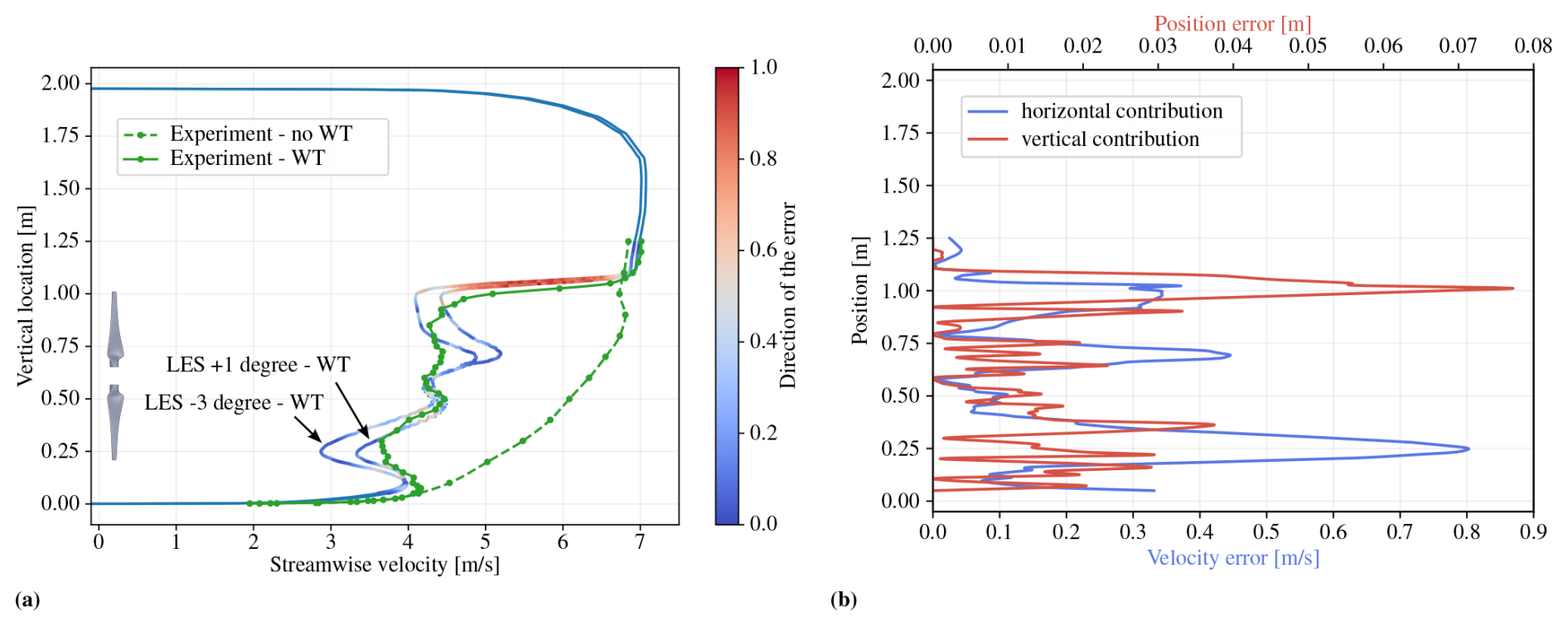
Figure 20 Error quantification for the velocity profile from Fig. 19 at location 2. (a) Orientation of the errors, where 0 denotes a horizontal contribution (in velocity) and 1 denotes a vertical contribution (in height). (b) Quantification of the errors per direction for the curve with pitch −3°.

To quantitatively compare each numerical result with the experimental data, the metrics described in Sect. 2.1.2 are employed, as presented in Table 1.

Table 1 Errors for the velocity profile at location 2: LES with wind turbine compared to experiment.

However, this alone does not fully explain the source of the discrepancies. To better understand them, the error is broken down into two categories: positional errors (vertical) and velocity errors (horizontal). These are illustrated in Fig. 20, which illustrates that most of the errors are in velocity, except around the height of 1 m where the curve shows higher errors in position.

Similarly, results are extracted at location 3 and compared in Fig. 21. For this position, measurements could not be repeated to reduce the random uncertainties due to the limited availability of the wind tunnel and hence the error bars are larger.

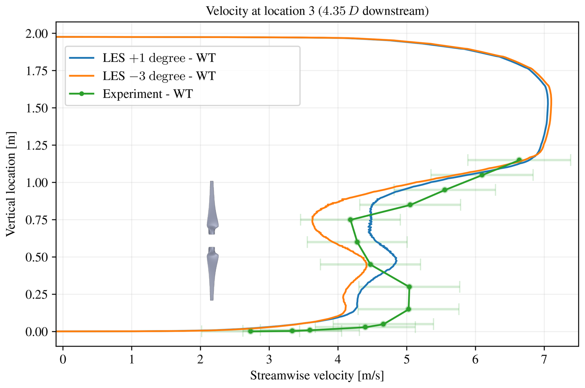
Figure 21 Velocity profile comparing the LES simulation using two pitch angles with the experiment at location 3 (4.35 D downstream of the wind turbine).

Both experimental and numerical curves show smoother gradients in velocity, as expected due to the enhanced mixing of the wake at this further downstream position. As a result, the slope of the transition between the free flow and the wake is not as sharp. In the lower region <0.4 m, a noticeable difference is observed between the experiment and both numerical cases. This is likely due to the change in ground roughness in the wind tunnel, which is not accounted for in the simulation. In the bulk of the wake, there is a difference of ∼ 0.9 m s⁻¹ between the two numerical cases, and how well these compare with the experimental data remains unclear due to the large uncertainty in the measurement.

Table 2 Errors for the velocity profile at location 3: LES with wind turbine compared to experiment.

5 Deformation of the blades

The deformation of wind turbine blades plays a crucial role in the overall aerodynamics and performance of the turbine. Under the influence of aerodynamic forces, gravitational loading, and centrifugal forces, the blades experience elastic deformations that can significantly alter the flow characteristics around the turbine. This deformation can affect key parameters such as angle of attack, lift, and drag of the blade sections, leading to changes in the aerodynamic efficiency and power production of the turbine. The experimental wind turbine designed for the present work has printed blades made of plastic (PLA+) that is highly flexible and hence can lead to a different flow behavior compared to a rigid configuration. The methodology used to explore blade deformation of the current experimental model uses both numerical simulation and experimental comparison.

5.1 Numerical approach: structural solver

Starting with the numerical approach, we employ a structural solver to translate the aerodynamic loads applied to the wind turbine blade into resulting deformations. The solver calculates how the blade deforms under a defined loading condition. The primary goal is to determine the deformation in the flapwise direction (perpendicular to the plane of rotation), the spanwise direction (in the direction of blade rotation), and the combined out-of-plane component of twist, which arises from the interplay of both flapwise and spanwise bending.

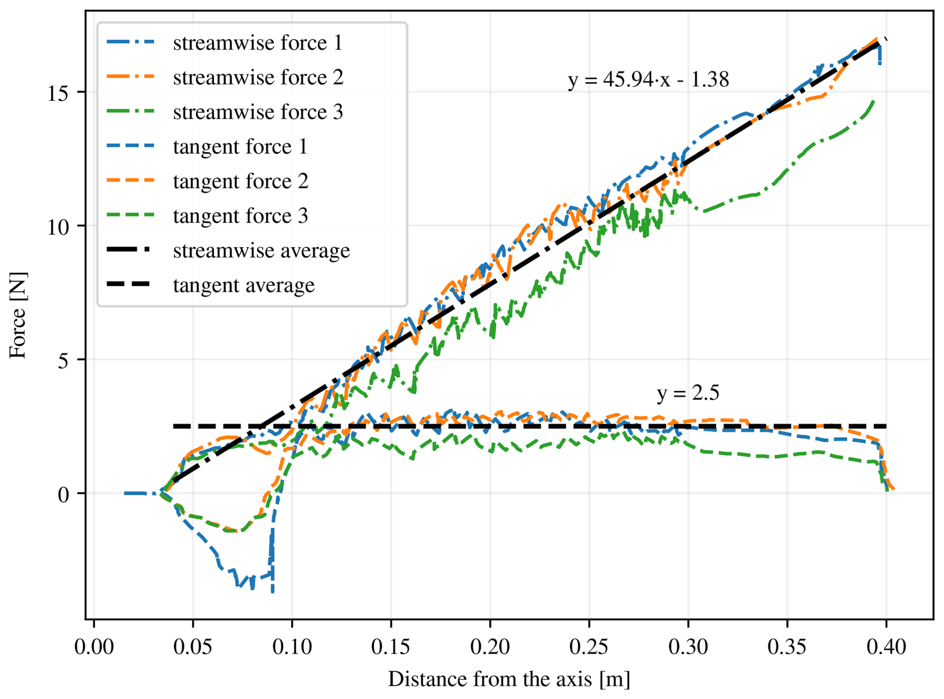
Figure 22 Distribution of forces along the blade in the stationary frame of reference from the LES simulation using the cALM.

The applied load includes the aerodynamic lift and drag on each blade section, a centrifugal force due to the rotation (which is also significant considering the rotational speed). The component of gravity is here negligible. Based on previous work on the topic for large wind turbine in turbulent wind with unsteady loads (Trigaux et al., 2024a), it appears that approximating the flow behavior using the average aerodynamic load already provides good results for the blade mean deformation. In this study, we therefore use the average aerodynamic loads to compute the blade deformation.

Figure 23 3-D CAD of the deformed blade, with indications for the forces applied to it.

The distribution of forces along the blade could not be obtained experimentally, so the values are exported from the previously shown LES with the cALM. Those forces along the blades are shown in Fig. 22 for the axial (streamwise) direction and the tangential (rotational) direction. Here, an instantaneous snapshot is shown. The axial forces increase linearly with radius, while the tangential forces remain relatively constant. This is a result of the blade design and is expected to showcase this behavior. Each curve represents an individual blade; one of them experiences a lower amplitude of the force applied because it is in the lower part of the boundary layer where the flow velocity is lower. General fluctuations are attributable to flow turbulence, while an additional effect can be observed in the region between 0.3 and 0.4 m, where the curve becomes more linear; this behavior is linked to the tip refinement, which reduces the Gibbs phenomenon. Another particular aspect visible here is that, at 0.4 m, the loading stops abruptly: this is not typical of most actuator line methods and is again due to the way the cALM was implemented and which allows for a sharp transition (when the mesh is refined enough at the tip). This provides a better flow representation of the tip vortex, and it reduces the error in the computation of the power produced. For simplicity, the distribution of forces is approximated using the two lines in Fig. 22, which then represents the average load used in the structural solver.

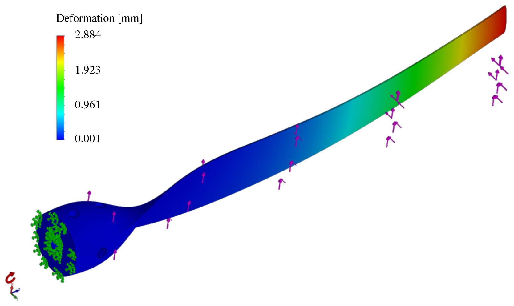
These forces are applied to the blade geometry, resulting in a deformation shown in Fig. 23. In this figure, the arrows represent the forces applied, with the vertical ones representing the constant tangential forces, the diagonal ones representing the axial forces, and the red arrow at the base indicating the rotation of the blade inducing a centrifugal force. The gravity component is ignored. The fixture of the part is represented with green arrows for the anchor point.

The geometry used for the structural solver is the CAD used for printing the blade. The material properties used in the simulation are provided from Iron Boar Labs Ltd. (2021); Ferreira et al. (2017). There are however some differences between the intended design and the resulting 3-D printed blade. The blade was printed vertically, starting at the root. The outer layer, shaping the aerodynamic profile, is printed from a continuous filament, with the goal of having a better surface for aerodynamics. With this printing method, the inside of the blade consists of a honeycomb pattern, which is more compliant than a solid block. It is thus expected that the physical blade deforms slightly more than the simulated one.

The blade deforms mostly in the flapwise direction (the most compliant direction), as shown in Fig. 23, where this deformation is highlighted with arrows. This behavior is expected since the majority of the axial loading acts in this direction. The largest deformation occurs at the blade tip, where a maximum deflection of 2.88 mm is predicted.

5.2 Experimental approach: camera measurement

A measurement of the experimental deformation of the blades provides further insights, complementing the numerical prediction. A significant uncertainty from the structural solver prediction comes from the fact the real blade is partly hollow, and hence it is deformed more than the simulation results. The goal of this experiment is to measure the flapwise deflection at the tip and compare it to the simulation.

For this study, the wind turbine was placed in the wind tunnel, as described in Sect. 2, with a camera placed outside of the wind tunnel, perpendicular to the plane of rotation. First, a calibration pattern was placed in front of the wind turbine, as shown in Fig. 24a. This calibration pattern is placed at the center of the wind turbine to avoid distortion due to perspective. The wind turbine was then rotated slowly manually, without any flow, to record a baseline (location of the blade tip when not loaded). The wind turbine is then operated with the wind tunnel turned on (as described in Sect. 2). The camera recorded a video with the blades loaded in their defined operating condition.

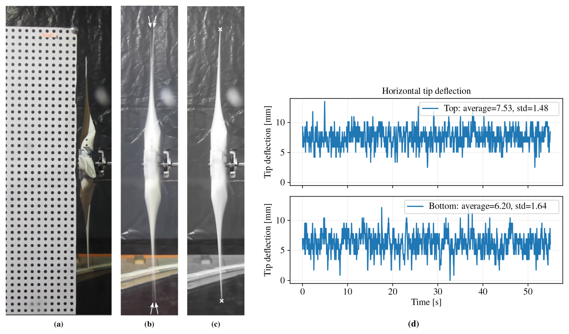
Figure 24 Measurement of the blade deflection. (a) Picture of the calibration of the camera. (b) Overlay shown of the unloaded and loaded blades. (c) Frame shown with the blade tip detection. (d) Deflection of the tip at the bottom and at the top shown as time series.

In Fig. 24b, the two videos are overlaid. A ghosting effect is used on the unloaded case to show the blade tips at the top and bottom in their initial state, and a single image from the video of the loaded case is used to show the deformed state. The initial state is more faint but outlined by an arrow on the image.

A detection algorithm was developed to measure the position of the blade tip at the top and at the bottom. A snapshot of the resulting video with the detected tips is shown in Fig. 24c, where an “x” indicates the detected tip. The algorithm for computing the blade deflection consists of the following steps:

• Convert the video to black and white, and increase the contrast such that the white blade is clearly identifiable against the black background.

• A horizontal line is used at the height of each tip (top and bottom) to restrict the detection zone. An additional restriction zone in the horizontal direction is used to avoid outliers of a reflection in the background.

• On these two lines, the maximum brightness point determines the position of the blade.

This algorithm is applied to each frame. Finally, a manual check of the video ensures that the algorithm correctly identified the tip at each frame.

At each frame from Fig. 24c, a distance is obtained from the unloaded point to the tracked point of the frame: this distance is in pixels. The calibration pattern then allows one to convert pixels to millimeters to quantify the deflection of the tip in the flapwise direction. The evolution of this deflection is provided in Fig. 24d. The mean blade tip deflection is 7.5 mm at the top and 6.2 mm at the bottom (lower, as it is less loaded), which is significantly more than the predicted 2.9 mm obtained when assuming that the blade is not partly hollow. Yet, it amounts to 2.0 %–2.4 % of the blade's active span (which is ∼ 30 cm), which is still moderate even though the PLA+ material used for the blade is rather flexible.

6 Discussion

The comparison between experimental measurements and LES using the cALM reveals both the strengths and the limitations in reproducing the loading and near-wake dynamics of a model-scale wind turbine. In the results assessing the influence of the blade pitch angle presented in Sect. 4, the wake at location 2 (1.41 D downstream; see Fig. 19) exhibits more variation in the vertical direction as compared to location 3 (4.35 D downstream; see Fig. 21), as expected. Since location 2 is closer to the wind turbine and is more challenging to reproduce numerically, it was the main focus in this investigation. At this location, the numerical results capture well the intricate wake structure, with a notable agreement in the overall velocity deficit. This agreement is also attributed to the accurate reproduction of the inlet conditions (Sect. 3.2), which plays a crucial role in shaping the near-wake behavior. A direct comparison of power between experiment and simulation is not straightforward, as the experimental measurements correspond to electrical power on the DC bus, while the LES results represent aerodynamic power extracted from the flow. The experimental setup includes several loss mechanisms (mechanical transmission and power electronics), so only an order-of-magnitude agreement can be expected. In Fig. 19, the overall velocity deficit between experiment and simulation shows good agreement, indicating comparable thrust levels in both cases.

A key strength of the cALM implemented in this study (in Sect. 3.3), is its ability to replicate the sharp velocity gradient between the free stream (>1.1 m) and the wake (<1 m). This is made possible by disabling the tip force spreading in the ALM and by using a mesh that is sufficiently refined there. In the error quantification shown in Fig. 20, this region appears with a deviation in height of 7.5 mm. While this error is greater than the measurement uncertainty, it remains modest enough for most applications.

The multiple changes in the derivative around hub height (0.6 m) are also fairly well captured, highlighting the influence of the nacelle-induced drag and the limited energy extraction by the blade root.

However, a notable deviation near the blade root (0.7 m) underscores a key limitation of the cALM: the assumption that 2-D airfoil polars can adequately represent the blade aerodynamics. In this region, the complex geometrical transition (from blade airfoil to ellipse to circle) and 3-D nature of the flow invalidates this assumption, leading to discrepancies between simulation and experiment. This limitation is critical when analyzing the near-wake region.

To better interpret the effect of blade pitch, the spatial influence of the different modeling components was assessed at location 2 (1.41 D downstream). It is observed that the nacelle primarily affects the wake in the region between 0.52 and 0.65 m, while the blade root region, where ALM assumptions are known to be less reliable, influences the flow between 0.65 and 0.75 m, as well as between 0.42 and 0.52 m. The remainder of the swept area lies outside these regions and is governed by the actuator line formulation in a regime where it is generally considered valid.

The influence of the blade pitch angle was then investigated. Near the tip, the +1° pitch case aligns more closely with the experimental near-wake data, while near the root, the −3° pitch case shows a better agreement. However, since the root region and parts of the nacelle-affected flow are known to be influenced by modeling limitations, these areas are expected to exhibit additional deviations that are not primarily driven by pitch effects.

In contrast, in the remaining portion of the swept area where the ALM assumptions are expected to hold, the observed differences between pitch cases remain clearly visible along the blade span. In these regions, including those not affected by nacelle or blade-root influences, the variations are consistent with changes in blade angle of attack induced by the pitch modification. Deviations in the root and nacelle-affected zones are additionally influenced by known modeling limitations. This suggests that the pitch sensitivity is primarily captured in regions where the model is valid, while discrepancies near the root are dominated by known modeling limitations.

This behavior further reflects the inherent limitations of the ALM, which relies on the local airfoil chord direction, angle of attack (evaluated at the aerodynamic center), and velocity magnitude, while assuming a two-dimensional cross-sectional flow and using simplified airfoil polars. These assumptions make it challenging to fully reproduce the experimental blade loading. However, no definitive conclusion on loading discrepancies can be drawn, as the experimental blade loading distribution was not measured.

The blade flapwise deformation was analyzed in Sect. 5. Experimentally, the tip deflection was moderate (6.2 mm bottom, 7.5 mm top), influenced by the sheared inflow profile. The structural model predicted an even smaller deflection of 2.9 mm, which is most likely due to the solid blade assumption in the simulation, whereas the experimental blade was partly hollow with a honeycomb structure. We also stress that PLA+ is a plastic that has more flexibility than a composite material. Despite this, the observed deformation amounts to only 2.0 %–2.4 % of the blade active span (which is ∼ 30 cm).

Overall, the measured deviations in the wake profile are most likely attributable to blade deformation, which leads to variations in the angle of attack along different spanwise locations of the blade. However, it is important to note that several numerical factors may also contribute to these discrepancies, including local velocity sampling resolution, the use of two-dimensional airfoil polar data, and numerical dissipation introduced by the sub-grid scale model. To better isolate the origin of these deviations, experimental measurements of the spanwise blade loading using strain gauges would provide valuable insight. However, this investigation is left for future work.

7 Conclusions

In this study, we designed, constructed, and experimentally characterized the TWIST (Turbine for Wind-tunnel Investigation and Scaled Testing), providing a new model-scale wind turbine and a high-resolution dataset for near-wake velocity and blade deformation measurements in a controlled wind tunnel environment. In parallel, a novel and improved continuous ALM (cALM) was implemented in Nek5000, incorporating capabilities such as reduced tip-force spreading and the avoidance of radial averaging, with the aim of enhancing physical fidelity. Particular care was taken to reproduce the experimental inlet flow conditions in the LES, matching both the mean velocity profile and turbulence intensity to ensure a meaningful comparison between numerical and experimental results.

The comparison shows that the cALM approach is capable of capturing the essential features of the near-wake region, where flow structures are highly sensitive to modeling fidelity. At 1.41 D downstream, both experimental and numerical results show a complex velocity profile with significant vertical variation. The overall velocity deficit is fairly well captured, and the sharp transition between the free stream and the wake is properly reproduced. This agreement is supported by the fine mesh resolution and by the ability of the cALM to represent blade tip effects with limited artificial smoothing. The effect of the hub is also accounted for using a distributed drag force within an ellipsoid, and the blade root region is included in the model. However, deviations near the blade root persist, highlighting intrinsic limitations of ALM, which relies on 2-D airfoil polars, whereas the blade geometry in this region transitions rapidly and induces complex three-dimensional flow.

The sensitivity studies presented here further clarify the model behavior and the origin of remaining discrepancies. The blade pitch angle study demonstrates the strong influence of operating conditions on wake development and confirms that the cALM captures the corresponding trends observed experimentally. In addition, blade deformation was investigated both numerically and experimentally, with measured deflections of 2.0 %–2.4 % of the blade active span. Although the PLA+ material is relatively flexible, such moderate deformation is unlikely to significantly affect blade loading or induce noticeable bend–twist coupling. This suggests that aeroelastic effects are not the primary source of discrepancies and that remaining differences are more likely linked to modeling assumptions, particularly in regions with strong three-dimensional flow such as the blade root. To better isolate these deviations, spanwise blade loading measurements using strain gauges would be valuable but are left for future work.

Overall, this work demonstrates the relevance of combining a dedicated experimental setup with targeted numerical developments to improve the understanding of wind turbine wake physics. The TWIST turbine and the associated measurements provide a valuable reference for controlled studies, while the cALM offers improved physical representation of key flow features. The consistency observed between simulations and experiments, together with the insights gained from the sensitivity analyses, supports the applicability of the proposed approach for investigating near-wake behavior under well-defined conditions. These results contribute to ongoing efforts toward more reliable and physically grounded wind turbine modeling.