the Creative Commons Attribution 4.0 License.
the Creative Commons Attribution 4.0 License.
 | 13 Aug 2019
Lidar estimation of rotor-effective wind speed – an experimental comparison
Jakob Mann
Lidar systems have the potential of alleviating structural loads on wind turbines by providing a preview of the incoming wind field to the control system. For a collective pitch controller, the important quantity of interest is the rotor-effective wind speed (REWS). In this study, we present a model of the coherence between the REWS and its estimate from continuous-wave nacelle-mounted lidar systems. The model uses the spectral tensor definition of the Mann model. Model results were compared to field data gathered from a two- and four-beam nacelle lidar mounted on a wind turbine. The comparison shows close agreement for the coherence, and the data fit better to the proposed model than to a model based on the Kaimal turbulence model, which underestimates the coherence. Inflow conditions with larger length scales led to a higher coherence between REWS and lidar estimates than inflow turbulence of smaller length scale. When comparing the two lidar systems, it was shown that the four-beam lidar is able to resolve small turbulent structures with a higher degree of coherence. Further, the advection speed by which the turbulent structures are transported from measurement to rotor plane can be estimated by 10 min averages of the lidar estimation of REWS. The presented model can be used as a computationally efficient tool to optimize the position of the lidar focus points in order to maximize the coherence.
- Article
(6163 KB) - Full-text XML
- BibTeX
- EndNote


The control system is an integral part of a wind turbine and has substantial influence on its behaviour. Its aim is to maximize the power production while keeping the turbine structural loading within the design limits. In order to decrease the levelized cost of energy, several novel sensors and control strategies have been proposed. One of them is a lidar-assisted pitch controller and one of the first was introduced by Harris et al. (2006). It utilizes nacelle- or spinner-mounted lidar systems to retrieve information about the inflow. In contrast to traditional feedback (FB) control of rotor speed, disturbances in the inflow can be measured by the lidar before they affect the turbine. For collective pitch control, a simple approach is to add a feedforward (FF) pitch angle demand (βFF) based on lidar measurements to the FB demand (βFB) derived from the rotor speed deviation from its desired value (Ωr); see Fig. 1.
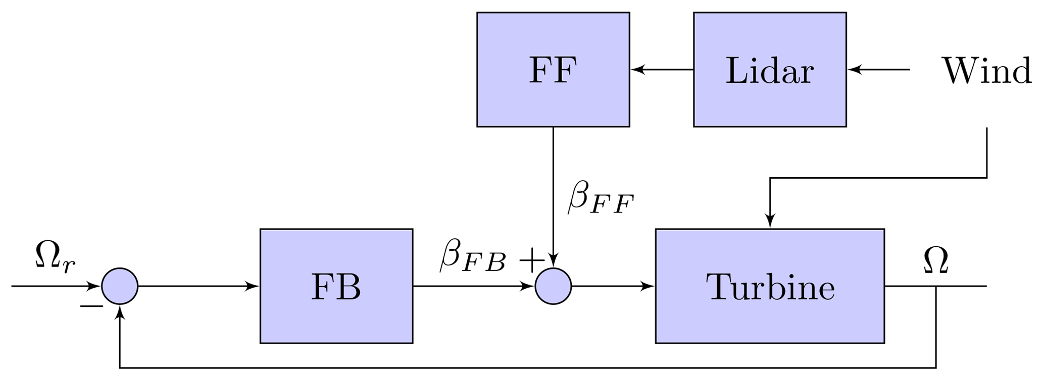
Figure 1Block diagram of a lidar feedforward collective pitch controller to assist a traditional feedback controller.
For such a controller, the important information about the wind is the rotor-effective wind speed (REWS) (veff), which can be defined in several ways (Soltani et al., 2013). One definition states that the REWS is the average longitudinal wind speed component over the entire rotor plane, which is used in this work. Alternatively, the average of the longitudinal wind speed with different weights for the hub or tip regions of the blade can be used. In the ideal case of perfect lidar measurements of veff and turbine modelling, disturbances can be completely rejected and optimal rotor speed control can be achieved (Dunne et al., 2011). However, this is not achievable in reality and important shortcomings of the lidar systems are
-
the contamination from lateral and vertical wind speed components,
-
the spatial averaging due to the lidar's probe volume,
-
the scarcity of measurement points in the rotor plane
-
and the uncertain estimation of the time delay between lidar measurement and disturbance arrival at the rotor.
Thus, it is important to optimize the measurement positions of the lidar to maximize the correlation between lidar measurement and REWS for which flexible and computationally efficient models are required.
Previously, Schlipf et al. (2013) presented an analytic correlation model in the frequency domain to calculate the magnitude-squared coherence and transfer function between a lidar and a turbine using the Kaimal spectral model and an empirical exponential decay coherence model of the longitudinal wind component for separations perpendicular to the flow. The turbulence model is defined in the IEC-61400-1 standard (IEC, 2005). The advantage of this approach compared to simulations in time domain is the reduced computational effort. However, integrating certain lidar properties becomes complicated if done analytically. For example, the spatial averaging effect of the lidar has not been integrated into the model. Therefore, Schlipf et al. (2013) also proposed a semi-analytic model, where properties of the lidar can be added in the frequency domain, and coherence and transfer function can then be calculated. The model has been extended by Haizmann et al. (2015a) to include linear rotor-effective horizontal and vertical shear estimation. Different optimal focus positions were found for REWS and shear estimations, implying that a compromise needs to be found if both quantities are wanted. Another optimization was performed in Schlipf et al. (2015), where additionally the wind evolution and constraints from the controller were considered. In Simley and Pao (2013b), a similar semi-analytic method was presented to calculate the correlation between a spinner-mounted lidar and blade-effective wind speeds. The difference lies in the fact that spinner lidars rotate with the rotor and thus sample the wind field rotationally. In a more recent publication, the theoretical and practical aspects of lidar optimization are addressed (Simley et al., 2018). The results of the optimization of several lidar setups based on different optimization metrics are presented.
Comparisons between data gathered during field experiments and models were conducted in several studies. In Schlipf et al. (2013), the previously mentioned semi-analytic model was compared against data gathered on National Renewable Energy Laboratory (NREL)'s Controls Advanced Research Turbine (CART2) test turbine. The measured and modelled transfer functions showed very good agreement, and the maximum coherent wavenumber, defined as the wavenumber where the coherence reaches a value of 0.5, was 0.06 rad m−1 for both methods. A similar comparison was performed on NREL's CART3 turbine by Scholbrock et al. (2013), where deviations between model and measured data were observed. As a possible explanation, interference of the guy wires of a close-by meteorological mast with the lidar was given. In a later experiment on the same turbine with a different lidar system, Haizmann et al. (2015b) found great agreement between data and model. For this lidar, the maximum coherent wavenumber was found to be 0.03 rad m−1.
The integration of lidar measurements into turbine control by suitable controllers and their associated benefits have been the topic of various analyses. FF additions to FB controllers have been studied in, e.g. Laks et al. (2011); Dunne et al. (2011). A more sophisticated flatness-based controller was proposed in Schlipf and Cheng (2014), while individual pitch controllers have been considered in, e.g. Dunne et al. (2012). Model-predictive control approaches were examined in, e.g Mirzaei et al. (2013).
To verify simulated performance, field tests have been pursued. In Scholbrock et al. (2013), a pulsed lidar system was used on NREL's CART3 turbine. A collective pitch feedforward approach (similar to Fig. 1) was compared to a feedback controller only and load reductions at low frequencies (below 0.1 Hz) were observed. Damage equivalent loads (DELs) were reduced by approximately 2 % and 7 % for the tower fore-aft bending and the blade flapwise bending moments, respectively. A similar study was presented in Schlipf et al. (2014) using the CART2 turbine, where the blade and tower DELs were reduced by 10 %. However, periods where the lidar's vision was obstructed by hard targets showed an increase in DELs, thus emphasizing the influence of environmental conditions on lidar measurements. Another experiment on CART2 was performed by Kumar et al. (2015), where, besides adding a feedforward controller, the gains of the feedback controller had been reduced. Here, the load analysis showed that a reduction was achieved after reducing the feedback gains.
In this paper, we present a model of the coherence between REWS estimated from turbine and lidar measurements. The model uses the description of a turbulence field according to the model by Mann (1994), which allows to derive expressions of the auto- and cross-spectra numerically. In Sect. 2, these expression are presented along with the determination of REWS from field measurements at the turbine and from the lidar. Section 3 explains the test site and its characterization, while Sect. 4 shows the measurement results and the comparison with the presented model. The model can be used as a computationally efficient tool to predict the auto- and cross-spectra of REWS from turbine and lidar measurements and the optimization of the lidar focus point positions.
In this section, we present a coherence model between nacelle lidar systems and a wind turbine. The theoretical expressions to calculate the variances of turbine and lidar measurements have already been derived in Mirzaei and Mann (2016) and here we extend those to also calculate auto- and cross-spectra.
The fluctuating part of a three-dimensional (3-D) wind field can be represented by the vector field , where and refer to a 3-D spatial and wavenumber domain, respectively. We assume that the vector field u(x,t) is frozen and the fluctuations are advected by the mean wind speed, i.e. Taylor's frozen turbulence hypothesis (Mizuno and Panofsky, 1975) applies:
where is the mean wind speed along the advection direction x1. Thus, the dependence on time can be eliminated. The field u(x) can be written as a Fourier transform pair:
where an integral over the three-dimensional quantities, k or x, means the integral from −∞ to ∞ over all three components. The more rigorous Fourier–Stieltjes notation (Batchelor, 1953) was avoided due to brevity and clarity. The ensemble average of the absolute squared Fourier coefficients is the spectral tensor Φij(k):
where δ(.) is the Dirac delta function. Since , Eq. (3) can be written as
The advantage of using a three-dimensional spectral tensor Φij compared to one-dimensional spectra and coherences as in Schlipf et al. (2013) is that the problem of comparing lidar-derived wind speed estimates with rotor-averaged winds is a truly three-dimensional question. As we will see later, the lidar beams are focused at different locations measuring different velocity components and the resulting spectra can be naturally expressed as weighted two-dimensional integrals over the three-dimensional spectral tensor; see, for example, Eq. (22). In this paper, we use the spectral tensor model by Mann (1994) which is given analytically and only contains three adjustable parameters: αKϵ2∕3, L and Γ. The first is the spectral Kolmogorov constant αK (Monin and Yaglom, 1975) multiplied by the dissipation rate of specific turbulent kinetic energy density ϵ to the two-thirds power. This parameter gives the level on the spectra in the inertial subrange (Kolmogorov, 1941). The second parameter L is a length scale describing the size of the eddies containing the most energy. Finally, Γ is a parameter describing the deviation from isotropy which is caused by the mean shear usually present in the lower parts of the atmosphere. When Γ=0, turbulence is isotropic, while typical values in the atmospheric surface layer where most wind turbines are present are between 3 and 4 (Peña et al., 2010; Sathe et al., 2012; de Maré and Mann, 2014; Chougule et al., 2015). Even though the spectral tensor of Mann is given analytically, the usual one-dimensional spectra which are the ones measured by, for example, sonic anemometers, cannot be expressed in closed form but have to be numerically integrated1. This is where the Kaimal model has an advantage as the one-dimensional spectra are given as simple analytic expressions (Kaimal and Finnigan, 1994; IEC, 2005). However, each of the three velocity component spectra are described by two parameters (a length scale and a variance), making in total six parameters, and on top of that all coherences between velocity components also have to be specified. In the IEC standard, only the coherence of the longitudinal velocity is specified. That requires three new parameters, and if all coherences for all combinations of velocity components were to be described in the same way, which is necessary for the present investigations, the number of parameters would be overwhelming. Additionally, the Mann model is related to the physical equations of the flow, i.e. the continuity equation and a linearized version of the Navier–Stokes equations describing the effect of the shear on the turbulence. With these advantages, we feel confident that using the Mann model for these investigations is a sensible choice.
2.1 Overview coherence model
In this study, we have used an estimation of the coherence to evaluate the correlation between models and measurements. Specifically, we were interested in the magnitude-squared coherence between the REWS measured at the turbine and estimated from lidar measurements:
where SLL and SRR are the auto-spectra of the lidar and turbine estimates of REWS and SRL is their cross-spectrum. From time series measurements, these spectra were calculated over a 10 min period. The resulting frequency domain is converted into wavenumber domain by the use of Taylor's frozen turbulence hypothesis using . The wavenumber describes the size of a turbulence fluctuation where a small wavenumber indicates a (spatially) large fluctuation, and vice versa. The remainder of this section will present the methods to calculate the REWS and spectra. At the end, the model is compared against numerical simulations to validate the implementation.
2.2 REWS estimated from turbine measurements
The REWS veff is the defined as the longitudinal wind vector component averaged over the entire rotor plane:
where R is the rotor radius, and J1 is the Bessel function of the first kind, and where the Fourier transform of the velocity field has been introduced by Eq. (2). The rotor is positioned perpendicular to the x1 axis, i.e. no yaw misalignment.
To calculate the auto-spectrum of veff, we first work out the auto-correlation using Eq. (8):
Notice that we have complex conjugated the first term, which is allowable because it is real. Each complex term in the integral is therefore conjugated. We now change the product of integrals into a double integral and move the ensemble averaging inside this integral. Since the Fourier transforms of the velocities are the only stochastic variables in the expression, the ensemble average can be moved so it only embraces the product of and u1(k′). Now we use Eq. (3) to introduce the spectral tensor, and performing the integral over k′ leaves us with a single three-dimensional integral:
This equation is now inserted into the definition of the spectrum:
and the Fourier transform essentially annihilates the integral over k1 in Eq. (11), and we are left with the final two-dimensional integral expression for the auto-spectrum of veff:
To estimate veff from signals measured on the turbine, the approach in Østergaard et al. (2007) was followed. It is based on using the entire rotor as an anemometer and derives the rotor-effective wind speed by considering the turbine model characteristics and several measured signals. The methods gives the magnitude of an undisturbed wind field that creates the (unique) combination of power production, rotational speed and pitch angle at the turbine. Thus, there is no need to correct for the effect of turbine induction.
The entire turbine is modelled by a simple drive train model:
where J is the moment of inertia of the drive train, Ω is the rotational speed of the rotor, Qa is the aerodynamic torque produced by the rotor, Qg is the generator torque and Qloss is a collective term for the lost torque along the drive train. In our field experiment, torque measurements at the low-speed shaft (LSS) were performed. Thus, the measurements are taken before the gearbox and generator (where most of the losses occur) and we can replace in Eq. (14). The sampling rate of the turbine data was 1 Hz. Further a low-pass filter was used to reduce the influence of measurement noise in the estimation of . The aerodynamic torque is defined by
where ρ is the air density, is the tip-speed ratio (TSR), Cp(β,λ) is the power coefficient as function of pitch angle β and TSR. By solving Eq. (14) for Qa and substituting it in Eq. (15), we arrive at
With a measurement of the pitch angles, a lookup with linear interpolation can be used to find λ that satisfies Eq. (16), and by the definition of the TSR, the REWS can be estimated:
The necessary Cp(β,λ) surface can be precomputed. Details can be found in Appendix A. Note that issues of non-monotonicity of Cp(β,λ) in Eq. (16) can be avoided by performing the lookup on and not on Cp(β,λ). The air density has been calculated from pressure and temperature measurements on a nearby meteorological mast.
2.3 REWS estimated from lidar measurements
Lidar systems are able to measure the frequency shift of light backscattered at aerosols moving with the wind in the atmosphere. This frequency shift is proportional to the velocity of the aerosols, and thus the wind speed can be determined. The measurement of a continuous-wave lidar system can be expressed mathematically as the convolution of the line-of-sight (LOS) component of the wind vector and a weighting function given by the laser light intensity along the laser beam:
where xf is the position of the lidar focus point, n is the laser beam unit vector,
is the weighting function defined by the Rayleigh length zR, and df is the distance from the lidar system to the focus point. The Rayleigh length describes the shape of the probe volume through Eq. (19). Note that the probe volume of the lidar increases with focus distance, i.e. . The probe volume has an attenuating effect on the turbulent fluctuations of the wind field. Equation (18) is assuming that the first statistical moment is used to calculate the dominant frequency of the Doppler spectrum, which is a result of the Fourier analysis of the detected light signal. Different frequency estimators can yield less turbulence attenuation (Held and Mann, 2018). The Fourier transformation of the weighting function (Eq. 19) is and the auto-spectrum of the lidar measurement along a single beam can be expressed as
where ni refers to the components of the laser beam unit vector n and summation of repeated indices is implied. The implied sum () could also be written in vector and matrix notation as n⋅(Φn), where the parentheses indicate a product between a matrix and a vector n, and a ⋅ means the dot product. Details of the derivation can be found in Mirzaei and Mann (2016).
The typical setup of a nacelle lidar looking forward is shown in Fig. 4a. The lidar system sequentially probes several focus points in front of the rotor. Due to the limitation of measuring, only the LOS components of the wind vector assumptions are necessary to derive the REWS from the lidar measurements. Here, we apply the following assumptions: (1) no vertical components, (2) zero turbine yaw misalignment. Based on these assumptions, the REWS can be estimated from lidar measurements as the average of all vLOS velocities:
where b is the number of beams and α is the half-cone opening angle of the scanning cone (see Fig. 4a).
In wavenumber domain, the auto-spectrum of the REWS estimate from lidar measurement using Eqs. (21) and (18) can be written as
where the index k should not be confused with the wavenumber k. The details of the derivation can be found in Mirzaei and Mann (2016) with the only difference that they integrate over k1 to get the variance, whereas we do not in order to get the one-dimensional spectrum.
When evaluating Eq. (21) from field measurement, a correction of the slowdown in speed as the wind approaches the turbine is necessary. This correction is referred to as induction correction. First, we used an analytic solution for the flow speed reduction and diversion around the rotor (Conway, 1995). The model assumes an actuator disk model and laminar, uniform inflow with uniform, non-rotational loading. An example of the flow around a rotor can be found in Appendix B. The induction correction , where U∞ is the undisturbed free steam wind speed, can be defined from the calculated flow field at the focus positions of the lidar beams. Thus, the induction correction depends on lidar parameters, i.e. the half-cone opening angle α and the focus distance df, and on the operational point of the turbine, i.e. the induction factor a. The induction factor is determined from the measured 10 min mean REWS by the lidar, and a steady-state thrust curve is used to look up the thrust coefficient Ct. Then the relation is used to calculate the induction factor. The effect of the induction is assumed to be constant over a 10 min period.
Integrating the induction corrections into Eq. (21) yields
This represents measuring the wind speed component perpendicular to the turbine rotor even when the turbine is misaligned with the free-stream wind direction. A turbulent structure travelling along the mean wind direction, which is not aligned with the rotor axis if yaw misalignment is present, can arrive at the different position at the rotor than predicted by the model. The model assumes that the turbulent structures travel along the mean wind direction and that the turbine is aligned with that wind direction. However, in the case of small yaw misalignment, the shortcoming of the model can be assumed to be insignificant.
2.4 Determination of the cross-spectrum
Similarly, the cross-spectrum between the REWS and its estimate from lidar measurements veff,L can be calculated using
where Δx indicates the distance between rotor and lidar measurement planes. Details of the derivation of the previous two equations can be found in Mirzaei and Mann (2016). Note that it is assumed that the lidar system probes focus points simultaneously, which is a simplification of the sequential scanning performed by the actual lidar system.
2.5 Model implementation and validation against simulations
For the implementation of the model, a C++ code has been created to numerically solve Eqs. (13), (22) and (24). Adaptive cubature integration was used as an integration algorithm2. To validate the implementation, numerical simulations have been performed. At first, six random 3-D turbulence boxes with different turbulence seeds have been created according to the Mann spectral tensor (Mann, 1998)3. The boxes had dimensions of 2800 m × 64 m × 64 m using 8192 × 32 × 32 grid points per box and contained only the turbulent part of the wind field; i.e. the mean wind speed was zero. The lidar measurements have been simulated using Eq. (18); however, due to the finite size of the boxes, the integration has been truncated at ±10zR from the focus point; details can be found in Held and Mann (2018). The two lidar systems presented in Table 1 have been used. The rotor plane (with a diameter of 52 m) was discretized by 100 × 100 grid points.
The results of the coherence analysis can be found in Fig. 2. It can be seen that the coherence for the two-beam lidar drops at lower wavenumbers than the four-beam lidar. This is due to the greater coverage of the rotor plane using four distinct focus locations compared to only two for the two-beam lidar. Further, the comparison between the simulations and the model shows very good agreement. Some deviations remain, which can be attributed to using only six simulations when estimating the coherence.
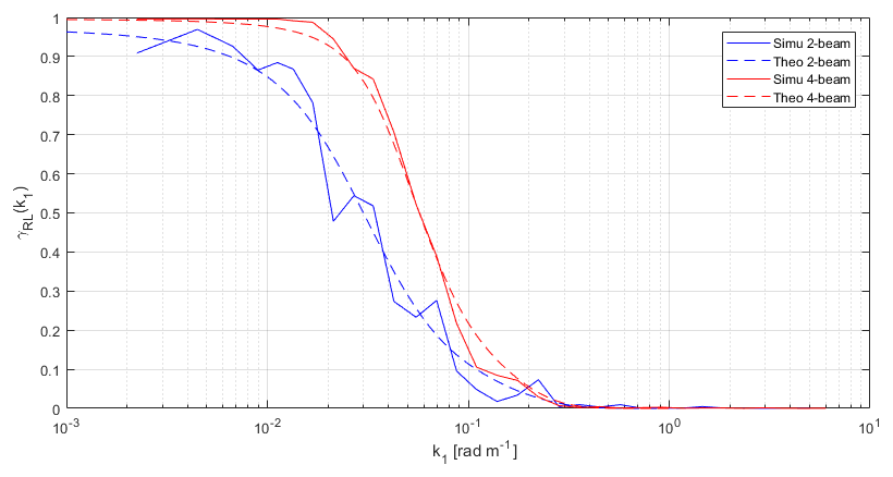
Figure 2Coherence between the estimation of REWS from the turbine and the lidar. The comparison between the numerical simulations (Simu) and the implementation of the model (Theo) shows very good agreement.
3.1 Instrumentation
Field measurements have been conducted at DTU's test site at Risø, located at the Roskilde Fjord in Denmark. The site consists of one row of wind turbines intended for testing, and several meteorological masts are installed around the turbines; see Fig. 3. During the experiments, only a Nordtank was operative, which is located at a distance of 215 m (4.1D) at an angle of 195∘ (from north). In general, there is a slight positive terrain slope from the fjord towards the turbines. To the east of the Vestas V52, some buildings and vegetation exist, while towards the west the turbine is facing flat fields and the fjord.
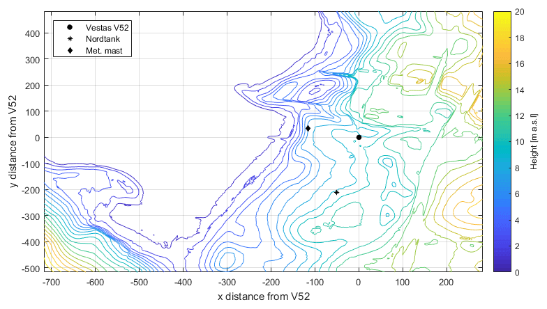
Figure 3Digital terrain model (DTM) of the DTU's test site at Risø, where the Vestas V52, its meteorological mast and the Nordtank turbine are indicated. Zone 32 UTM coordinates centred at the Vestas V52 turbine were used. The DTM data were obtained from the Danish Map Supply (Agency for Data Supply and Efficiency, 2018). The units on both axes are in metres.
For this experiment, two continuous-wave coherent Doppler lidars manufactured by Windar Photonics A/S have been mounted on a Vestas V52 turbine. The lidar systems, a two-beam and a four-beam lidar, are mounted on the nacelle of the turbine and have been staring forward to measure the inflow of the turbine. An illustration and a photo of the four-beam lidar can be seen in Fig. 4.

Figure 4(a) Illustration of the four-beam lidar focus locations on a cone with apex at the turbine nacelle. (b) Photo of the four-beam lidar mounted on the Vestas V52 turbine at the Risø test site.
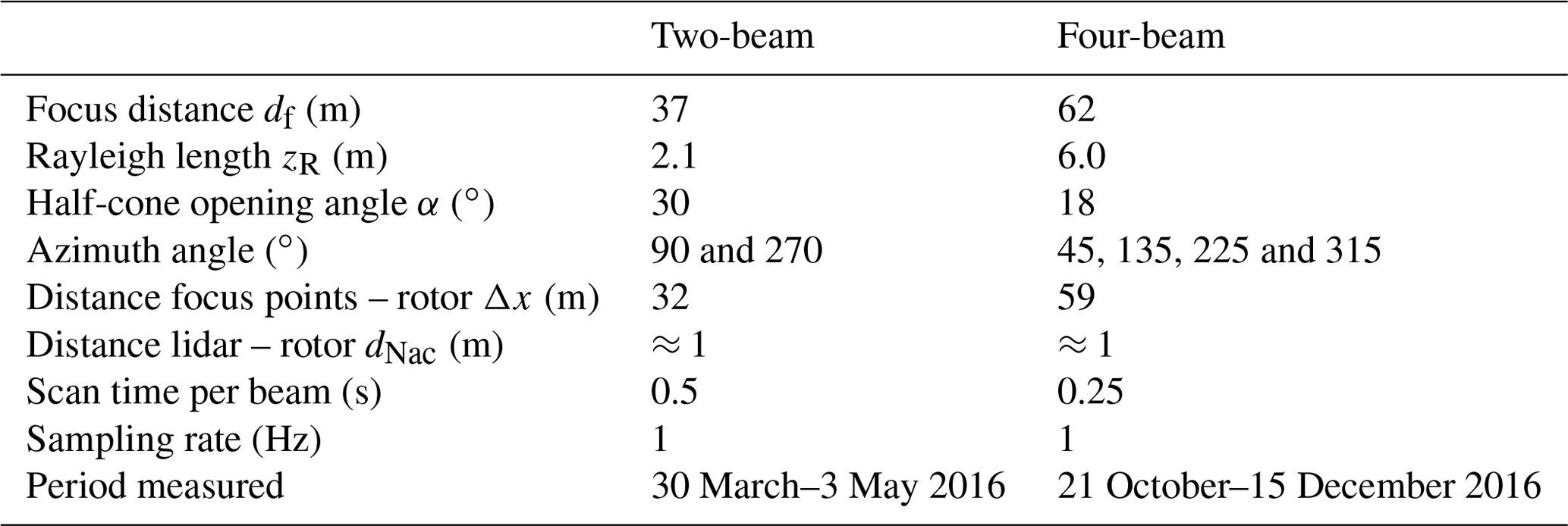
The specifications for both lidars can be found in Table 1. The two systems both contain one laser source located inside the nacelle and switch between the focus point sequentially. Each scan is completed in 1 s. Note the different Rayleigh lengths due to the different focus distances and the increased half-cone opening angle for the two-beam system. The azimuth angle refers to the position on the scanning cone surface. The position at the top of the cone is at an azimuth angle of 0∘. Hence, the two-beam lidar consists of two horizontal beams, while the four-beam lidar has one focus point in each quadrant of the rotor area. The distance between the lidar system and the rotor is dNac.
Table 1Information of lidar setup parameters and measurement periods. The azimuth angle refers to the position on the scanning cone surface with 0∘ being the top of the cone.
The Vestas V52 turbine has a diameter of 52 m and a hub height of 44 m with a rated power of 850 kW. It is heavily instrumented with several mechanical strain gauges, in particular a strain gauge setup to measure the torque on the low-speed shaft. Also a meteorological mast is located approximately 2.5D in front of it. To characterize the flow conditions during the experiment, a Metek P2901 USA-1 3-D sonic anemometer mounted at hub height was used. Further measurements from a Vaisala PTB110 air pressure sensor and a Vaisala R/H HMP 155 humidity sensor were used in addition to the temperature measurements from the sonic anemometer to calculate the air density.
3.2 Site characterization
The wind rose derived from wind direction and horizontal wind speed of the sonic anemometer measurements during the periods of the experiment is presented in Fig. 5a. The main wind direction is from the west, with winds coming from the Roskilde Fjord.
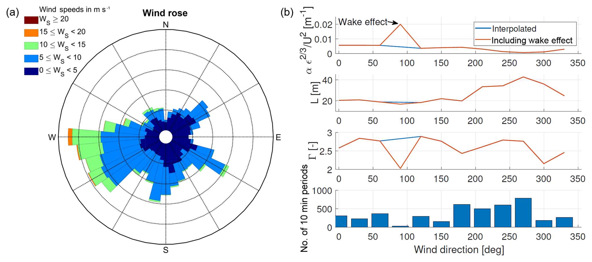
Figure 5(a) Wind rose gathered during the test periods at the Risø test site. (b) The three top panels show the result of fitting the Mann model to the calculated mean spectra as a function of wind direction. The bottom of panel (b) shows the number of acquired 10 min periods as a function of wind direction.
To get a clearer picture of the inflow conditions, the data set was grouped into sectors of 30∘ and the Mann model has been fitted to the average spectra in each sector. The fitting followed the procedure in Mann (1994) and was performed on the u, v, w spectra and the uw co-spectra. The spectra have been normalized by the mean wind speed squared. The model has three parameters: αKϵ2∕3, L is a length scale, and Γ is an anisotropy parameter as already explained in Sect. 2; for further details, see Chougule et al. (2015). The results of the three model parameter as function of wind direction can be seen in Fig. 5b. First of all, the effect of the wake from the Vestas V52 turbine on the sonic anemometer is clearly seen at a wind direction of 90∘. In this sector, a very high turbulent kinetic energy dissipation rate and a low anisotropy parameter were calculated. The results from this sector were disregarded and linearly interpolated. Secondly, two wind regimes can be identified. A region spanning from 330 to 180∘ shows a length scale L of approximately 20 m, while for the region from 210 to 300∘ larger length scales were fitted. Similarly, the normalized dissipation rate is higher in the first region compared to the second. This is in agreement with the terrain of the test site. The inflow for the first region is characterized by obstacles like buildings and tall vegetation. The second region faces open fields and the fjord fetch. The fit has also been performed for the Kaimal turbulence model, which is defined in the IEC 61400-1 standard (IEC, 2005). This model has one characteristic length parameter (Lk). Here, only the u, v and w spectra were fitted. The measured spectra have been normalized by their measured variance and the frequency domain has been converted into wavenumber domain. Then the model was fitted to the measured spectra by minimizing the combined mean squared error of the spectra.
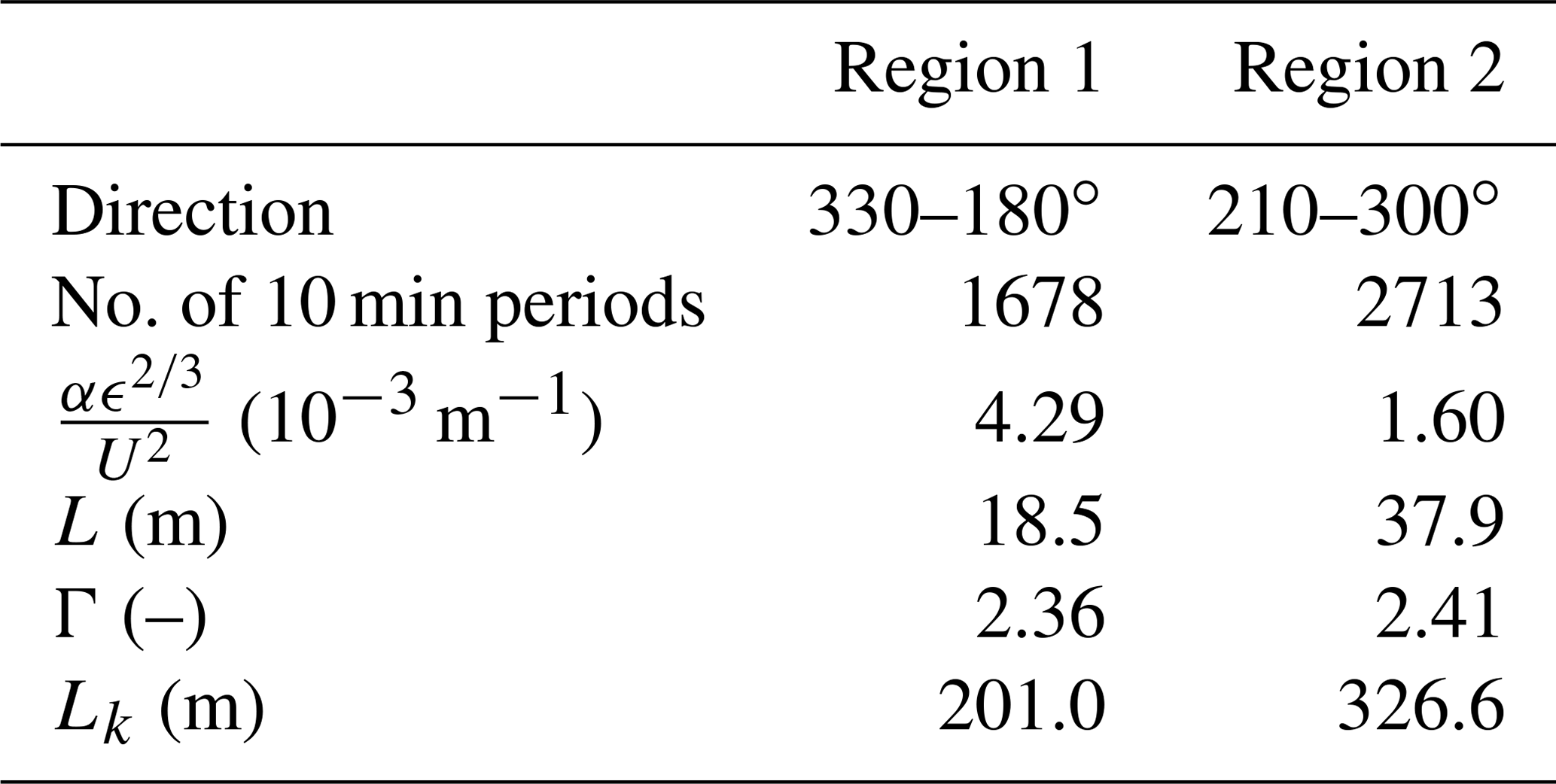
We separated the following analysis into two regions. The information on the two regions can be found in Table 2 including the averaged fits to the Mann model. Note that these two regions do not refer to the operational regions of the controller. More 10 min periods were obtained for region 2 due to the dominant wind direction from the west. The fitting results for the Kaimal model can also be found in Table 2. Similar to the Mann model, a larger length scale parameter was found for region 2. In Appendix C, the spectra and the fitted Mann model can be found. By dividing the data into two regions, as shown in Table 2, it was possible to identify two wind regimes with different turbulence parameter. It was also observed that binning according to atmospheric stability did not lead to significantly different spectra.
Table 2Measurement sectors and fitted Mann model , L and Γ) and Kaimal model (Lk) parameters.
The first step in the analysis of the results was to apply appropriate data filters, which reject measurements based on certain criteria. It was necessary to identify periods where the turbine was in a normal power production state. Thus, a lower threshold on the minimum power production (i.e. > 0 kW), minimum rotor speed (i.e. > 16 rpm) and maximum pitch angle (i.e. < 23∘) in a 10 min period were utilized. These thresholds were found by inspection of the available turbine data. This filter removed 52.8 % and 53.8 % of the data for the two- and four-beam experiments, respectively.
The filter applied to the lidar data consisted of a minimum number (> 90 % or 540 measurements) of available measurements on each beam in a 10 min interval. Unavailable measurements have been interpolated linearly. Instances where four or more consecutive unavailable measurements occurred on any beam were also discarded. Whether a measurement is available or not was decided internally by the lidar system and depends on carrier-to-noise ratio and the Doppler peak shape and area. After applying the turbine availability filter, this filter for the lidar data led to additionally discarding 2.9 % and 15.3 % for the two- and four-beam system, respectively. Since the four-beam system was under development during the field test, a higher unavailability is observed. Note that the interference by the blades is removed by the lidar systems based on the Doppler spectra, which have a distinct shape when laser light is reflected at the blades.
Additionally, inflow from all yaw position except from the wake sector () was considered because the lidar yaw misalignment measurements are biased in wake situations (Held et al., 2018). The yaw position filter led to an additional exclusion of 6.0 % and 6.3 % of the data for the two- and four-beam periods, respectively.
4.1 Comparison of mean wind speeds
Next, the 10 min average REWS estimates of lidar and turbine are compared to the sonic anemometer mounted on the meteorological mast. The comparisons for the two lidar systems and the turbine can be found in Fig. 6. Besides the previously mentioned data filters, only yaw positions where the turbine was facing the meteorological mast (i.e. a yaw heading of ) have been considered. It can be seen that both lidar systems agree well with the mast's sonic anemometers; linear least-square fitting results in a slope close to unity with no significant bias. This indicates that the corrections for turbine misalignment and induction are working as intended. Similarly, the correlation between mast and turbine also shows very good accordance with no systematic error.
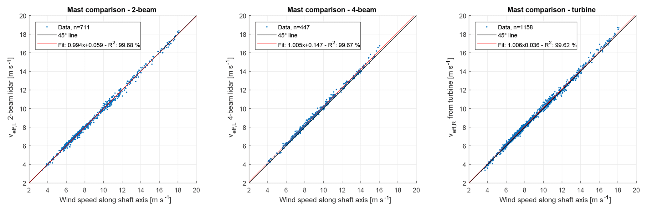
Figure 6Comparison of 10 min REWS estimates from of the lidars and the turbine to the meteorological mast's sonic anemometer. The data were taken from periods when the turbine was operational and facing the mast.
Corresponding comparisons are performed between the REWS estimated from the lidar systems and the turbine, respectively. The correlation plots can be found in Fig. 7. Analogous to the comparisons to the mast, theses comparisons also show that there is no systematic error between the two signals. Both linear fits show unity slopes and very small offsets. They are slightly worse than the comparisons to the meteorological mast, which can be explained by model inaccuracies when estimating the REWS when using turbine and lidar data.
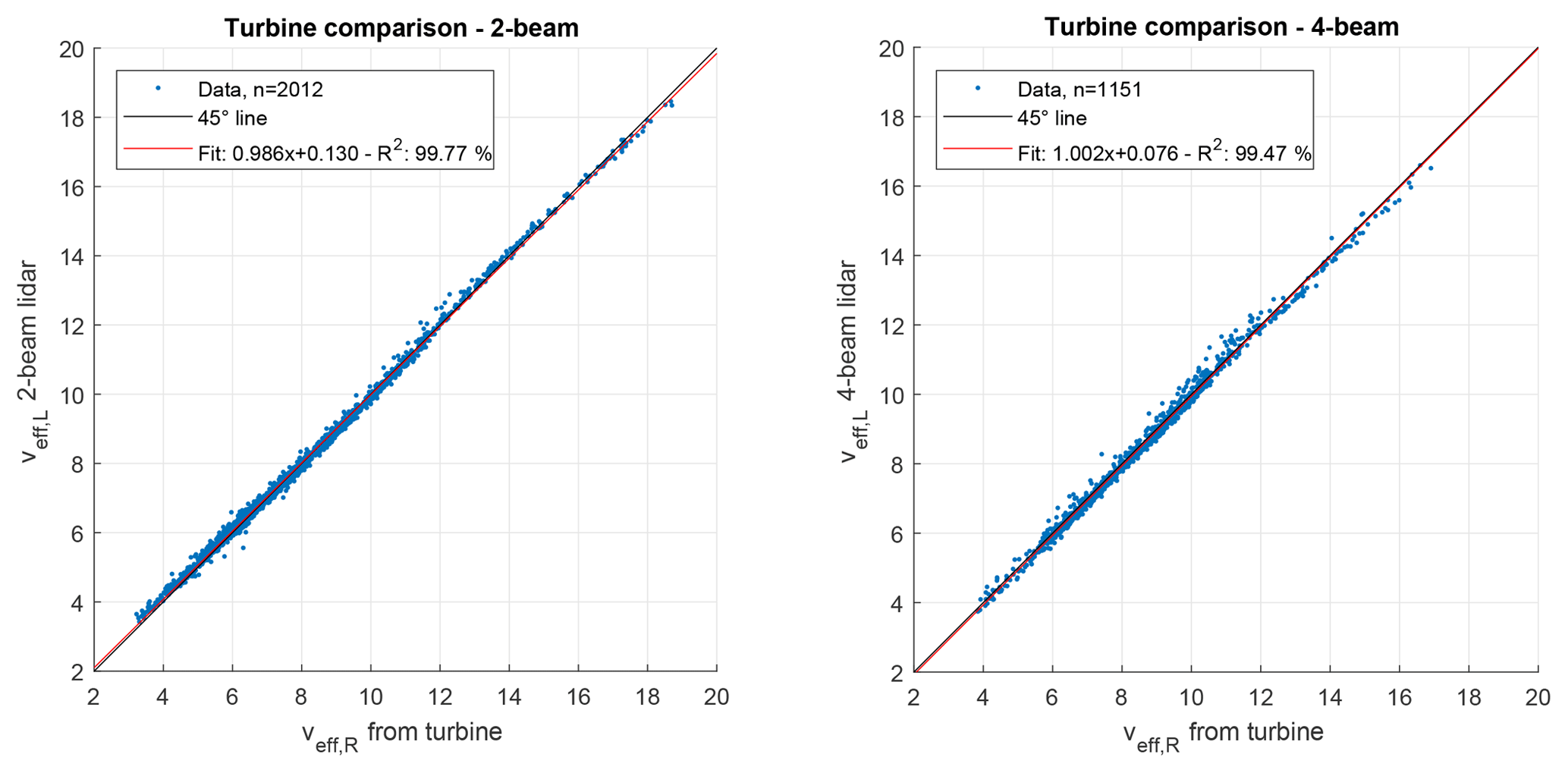
Figure 7Comparison of 10 min REWS estimates between the lidars and the turbine. Data from the wake sector and non-operational periods of the turbine were removed. All units are m s−1.
For illustrative purposes, the next plots in Fig. 8 show a single time series result for the lidar and turbine estimate of REWS. Both signals have a sampling rate of 1 Hz. In general, it can be seen that the fluctuations in REWS that were sensed by the rotor can also be measured by the lidar systems. For the two-beam lidar, larger deviations can be observed since this lidar probes the incoming wind field only at two locations. Fluctuations that occur at the top or bottom parts of the rotor cannot be measured. In the case of the four-beam system, a measurement in each quadrant is performed and gives a better estimate of the wind speed affecting the entire rotor. Further, the preview ability of the lidar systems also becomes apparent. Fluctuations can be measured before they affect the rotor.
4.2 Comparison of coherence
The effect of probing two versus four focus locations is now studied in wavenumber domain by comparing the squared coherences. The experimental data are also compared to two models: the model based on the Mann turbulence model introduced in Sect. 2 and the Kaimal turbulence model used in previous studies (Schlipf et al., 2013). As mentioned in Sect. 3.2, the analysis was split into two regions, of which one is disturbed by buildings or trees (region 1) and the other has an undisturbed inflow over open fields or the fjord's fetch (region 2).
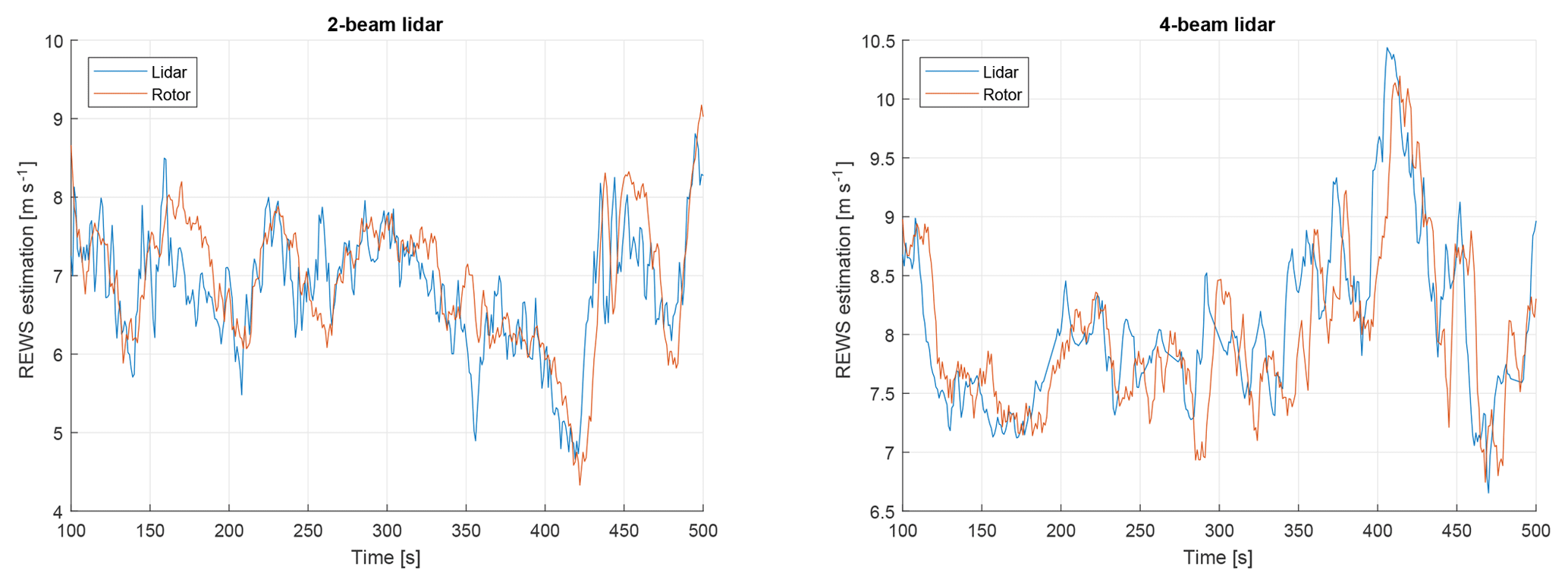
Figure 8Time series example of lidar and turbine estimates of REWS. A high degree of similarity between the signals can be seen. Also, the preview ability of the lidar system is evident.
The coherence analysis for region 1 can be found in Fig. 9. At first, it can be seen that the coherence of the two-beam lidar drops at lower wavenumbers than the coherence of the four-beam lidar, indicating that small fluctuations can be sensed more accurately by the four-beam system. Secondly, the measured data agree very well with the Mann turbulence model coherence. The Kaimal model, on the other hand, seems to give a slight underestimation of the coherence. The wavenumber at which the measured coherence dropped to the level of 0.5 is 0.027 rad m−1 for the two-beam and 0.051 rad m−1 for the four-beam system. These wavenumbers have been defined as the smallest detectable eddy size (Schlipf et al., 2018) and can be interpreted as the size of the eddy that is captured with an accuracy of 50 %. They are approximately 219.4 m (4.2D) for the two-beam and 122.5 m (2.6D) for the four-beams system, where the number in the brackets is normalized by the rotor diameter. Thus, by adding two additional focal points to a two-beam nacelle lidar system, the smallest detectable eddy size can be reduced by 44 %.
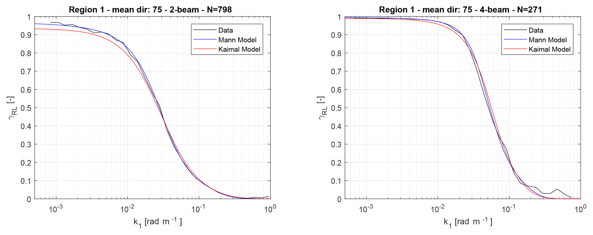
Figure 9Squared coherence between the REWS estimation of the lidar and the turbine for region 1. The two models are also included in the plot.
The results for region 2 are presented in Fig. 10. Here, very similar observations can be made. The coherence for the two-beam lidar drops at lowers wavenumbers compared to the four-beam lidar. The wavenumbers at γRL=0.5 are 0.032 rad m−1 and 0.056 rad m−1, and the smallest detectable eddy sizes are 198.8 m (3.8D) and 111.4 m (2.1D), respectively. This demonstrates once more a reduction of 44 % in the smallest detectable eddy size. Comparing these numbers to the results of region 1 shows that flow having larger length scale parameter is beneficial for lidar systems as the coherence drops at higher wavenumbers.
Equivalently to region 1, the Mann turbulence model fits very well to the measured data. There are however some slight deviations for both lidars in the region of 0.01 to 0.1 rad m−1, which could be caused by modelling inaccuracies of the assumed turbine model or general measurement noise in the turbine or lidar data. When comparing the experimental data to the Kaimal model, a larger mismatch is observed compared to region 1. These deviations could stem from the lack of the Kaimal model to represent 3-D turbulent structures. It is a 1-D model, which has been extended to represent 3-D turbulence by applying an empirical exponential lateral coherence model with completely independent velocity components, while the Mann model defines a full 3-D tensor model. Thus, the Mann model is able to represent better the three-dimensional structure of turbulence and thus give more realistic coherences.

Figure 10Squared coherence between the REWS estimation of the lidar and the turbine for region 2. The two models are also included in the plot.
To quantify the error between measured and model-derived coherence, we use the root-mean-squared error (RMSE) calculated from the data presented in Figs. 9 and 10. The RMSE is defined as
where refers to the measured coherence, is the model-derived coherence, and N is the number of data points. The model-derived coherence has been linearly interpolated at the available wavenumbers from the measurements. The RMSE is summarized in Table 3.
Table 3Comparison of the RMSE between measured and model-derived coherence for the two- and four-beam lidars in regions 1 and 2.
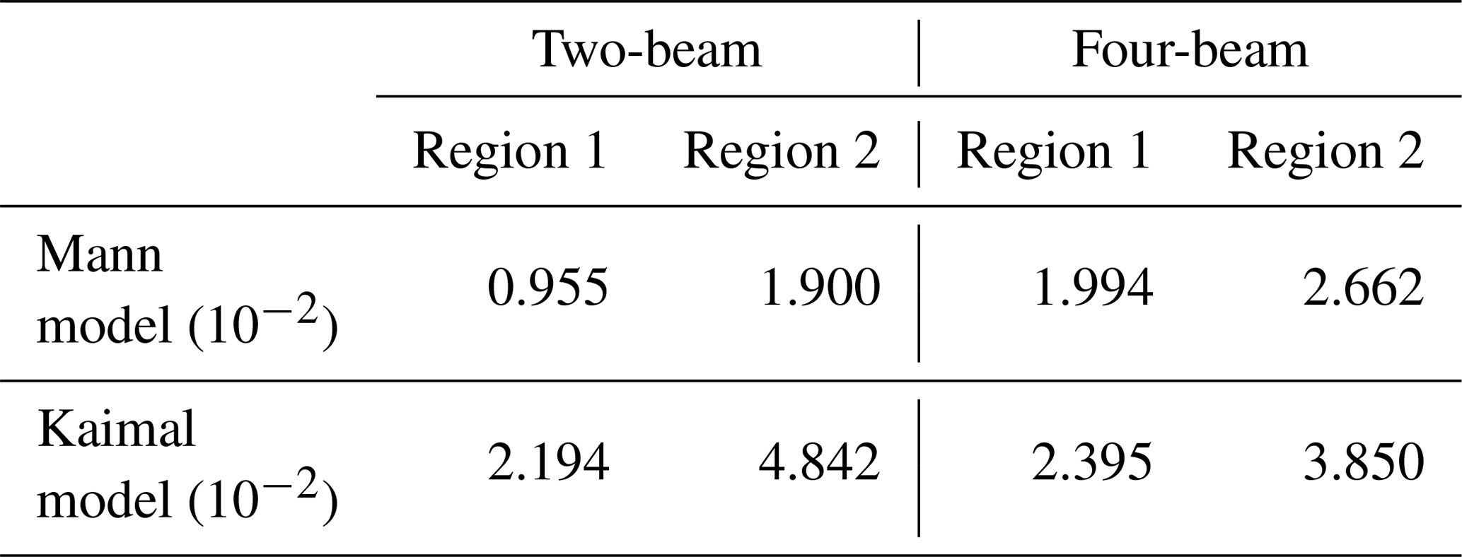
It can be seen that the errors between measured data and the model based on the Mann turbulence model are consistently lower than those of the model based on the Kaimal turbulence model. For the two-beam lidar, the errors are approximately twice as high, while the difference is slightly less for the four-beam lidar. Also, in region 2, the model based on the Kaimal turbulence model performs worse, which also can be seen when comparing Figs. 9 and 10.
Next, to better compare the measured coherence of the two- and four-beam lidar systems for regions 1 and 2, all measured coherences have been plotted in one figure. It can be seen that the coherence of the four-beam system drops at larger wavenumbers than the two-beam lidar due to probing the incoming wind at two additional positions. Differences between regions 1 and 2 can also be observed. For both lidars, the coherence measured in region 2 is higher than that in region 1. This can be explained by the larger turbulence length scale, which implies that there are more large-scale fluctuations in the flow. These large-scale fluctuations can be better resolved by both lidar systems.
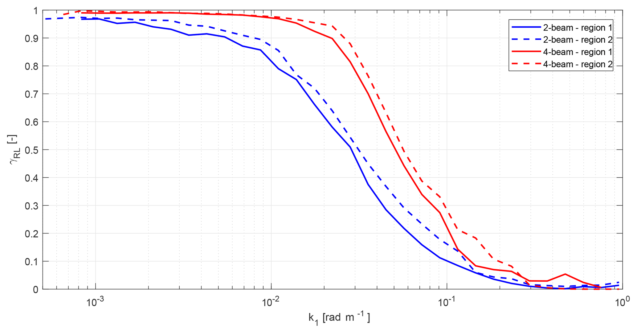
Figure 11Comparison of the measured coherence of the two- and four-beam lidars for regions 1 and 2.
Further, it is observed that even without the inclusion of the evolution of turbulence the model is able to predict the coherence very accurately. This implies that effect of disregarding turbulence evolution can be neglected. For bigger turbines, where larger focus distances are required, turbulence evolution might become more significant.
4.3 Time delay analysis
Next, the delay between lidar and turbine estimations of REWS is analysed. The delay stems from the perpendicular distance between the rotor plane and the measurement plane Δx. It depends on the advection speed,
where tScan is the time to perform one full scan, which is 1 s for both lidars, and , where dNac≈1 m is the distance between lidar mounting position and rotor. Uadv is the advection speed of the turbulent fluctuations, which is estimated by the 10 min average of the lidar-estimated REWS: .
Since the experiment was performed with very good time synchronization (with a maximum time delay of a few µs), it is also possible to calculate the delay between the two signals and compare it with expected delays based on the advection speed. The delay between the two signal has been calculated using the information theoretical delay estimator presented in Moddemeijer (1988). This method is based on splitting the two input signal into two parts: the past and the future and calculating the mutual information of two signals between the past and the future signals. The input signals are split in the middle of the time series. By shifting the signals relative to each other, the time delay which minimizes the mutual information is found. We have found that this method performs better than other delay estimators, namely the maximum index of the cross-correlation and the slope of the cross-spectrum. Due to the sampling rate of 1 Hz, calculated delays are discretized in steps of 1 s.
The result can be seen in Fig. 12. For the two-beam lidar, shorter delays are expected due to the smaller focus distance and larger half-cone opening angle. Still, the results for both lidars show great overlap between the measured delay and the delay expected from advection speed and the lidar geometry. The match of the measured and expected delays is worse for the two-beam lidar compared to the four-beam lidar. An overestimation of the delay for high wind speeds can be observed. However, the delay for high wind speeds is small and the delay estimator is affected by the low sampling rate of 1 Hz, which results in a delay resolution of 1 s. For low wind speed, an underestimation can be observed in the two-beam lidar data, which can also be identified to some extent in the four-beam lidar data. We speculate that this can be explained by faster wind direction changes at low wind speeds which lead to a turbine misalignment.
In general, towards high wind speeds, the available preview time provided by the lidar becomes smaller. The required preview time for the filtering is also shown for the two lidar setups. Low-pass filtering the lidar system is crucial to reject high-frequency fluctuations that are sensed by the lidar but not experienced by the rotor and if not filtered would cause detrimental pitch actuation. In this study, a first-order Butterworth filter is used following the approach presented in Schlipf (2015), though different filters have been proposed, e.g. a Wiener filter (Simley and Pao, 2013a). The delay of the filter is nonlinear but can be approximated by the delay at a certain frequency of interest (ωdelay=2πfdelay) (Schlipf, 2015):
where fdelay=0.0425 Hz was chosen as the frequency where the maximum of the rotor speed spectrum was observed. The cutoff frequency was determined from the coherence analysis presented previously at the point where γRL=0.5. The average over regions 1 and 2 was computed for both lidar systems and . This implies that the cutoff frequency changes with advection speed and an adaptive filter is required. For the two-beam lidar, it can be seen that there is sufficient time to perform the filtering at low wind speeds, but at high wind speed there is not enough preview time for the filtering. This results implies that a larger focus distance or smaller opening angle should be chosen for the two-beam lidar in order to be able to perform the low-pass filtering. For the four-beam lidar, it can be seen that the expected preview time provided by the lidar system is sufficient for the low-pass filtering.
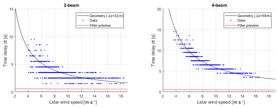
Figure 12Delay time analysis results for the two-beam and four-beam lidars. Delays and advection speeds are calculated based on 10 min averages. The required filter time of a first-order Butterworth filter is also shown.
In this study, we presented a model of the coherence between REWS estimated from turbine and lidar measurements. The underlying model of the 3-D turbulent field is the Mann spectral tensor and allows the direct calculation of auto- and cross-spectra of REWS estimations for lidar and turbine. It is compared to field data obtained from two continuous-wave lidar systems mounted on top of the nacelle of a wind turbine. To retrieve the turbulence model parameters, measured spectra from a sonic anemometer have been fitted to the spectral tensor. The comparisons of squared coherence show that the presented model fits the field data better than previously used models, which are based on the Kaimal model defined in IEC standard. Thus, this study gives confidence that the proposed model can accurately represent the important lidar properties and it can be used to optimize the lidar focus point positions to maximize the coherence between lidar and turbine. A common parameter used in the lidar optimization is the wavenumber where the coherence drops to a value of 0.5 (Dunne et al., 2014), which can be calculated precisely by the model.
We have found that larger turbulence length scales led to higher coherences between REWS estimated of turbine and lidar compared to inflow turbulence of smaller length scale. It was also shown that the smallest detectable eddy size can by reduced by almost 50 % when using the four-beam compared to the two-beam system. Further, the advection speed by which the turbulent structures are transported from measurement to rotor plane can be estimated from 10 min averages of REWS from lidar measurements. This is important information for the correct timing of the measured fluctuations of the lidar systems. In the case of the four-beam lidar, there is enough preview provided by the lidar to perform the necessary low-pass filtering, while the two-beam lidar lacks preview time for filtering for high wind speeds.
Since some of the physical mechanisms have not been modelled, future work includes additions to both the lidar and turbulence modelling. First of all, the evolution of turbulence as it travels from measurement to rotor plane has been neglected. An amendment of turbulence evolution to the Mann model has been proposed in de Maré and Mann (2016). The evolution will have the most influence on the small-scale fluctuations (Bossanyi, 2013) and including the effect will reduce the coherence. Hence, the model presented here can be considered an idealized case. On the other hand, only small differences were observed between data and model, implying that the evolution effect is small. For larger turbines, which require larger focus distances, this effect could be more severe. Secondly, the stability of the atmosphere was not considered; i.e. a neutral stratification was assumed. Extensions to the Mann model have been proposed to include effect of the atmospheric stability, e.g. Segalini and Arnqvist (2015) or Chougule et al. (2018). It should be noted that the discrete scanning of the lidar system and possible blade blockage effects have not been integrated into the model. Also, environmental conditions like the aerosol concentration, fog or precipitation have been disregarded.
The presented model in the current form can be applied to nacelle-mounted continuous-wave lidars and by modifying the spatial averaging of the lidar it can be extended to nacelle-mounted pulsed lidars as well. To cover spinner-mounted lidar systems, the rotational sampling effect of the lidar as it rotates with the rotor needs to be modelled.
The data are not publicly available since they contain confidential information owned by Windar Photonics A/S.
For the calculation of the Cp(β,λ) surface, an aerodynamic model of the Vestas V52 turbine was used. Aero-elastic simulations in HAWC2 over a domain of several pitch angles and TSR have been performed. A homogeneous, constant wind speed of 8 m s−1 was used and constant pitch angles and rotational speeds of the rotor were set during the simulation. Stiff tower and blades were used to avoid dynamic effects and calculate quasi-steady state Cp values. The resulting surface can be found in Fig. A1.
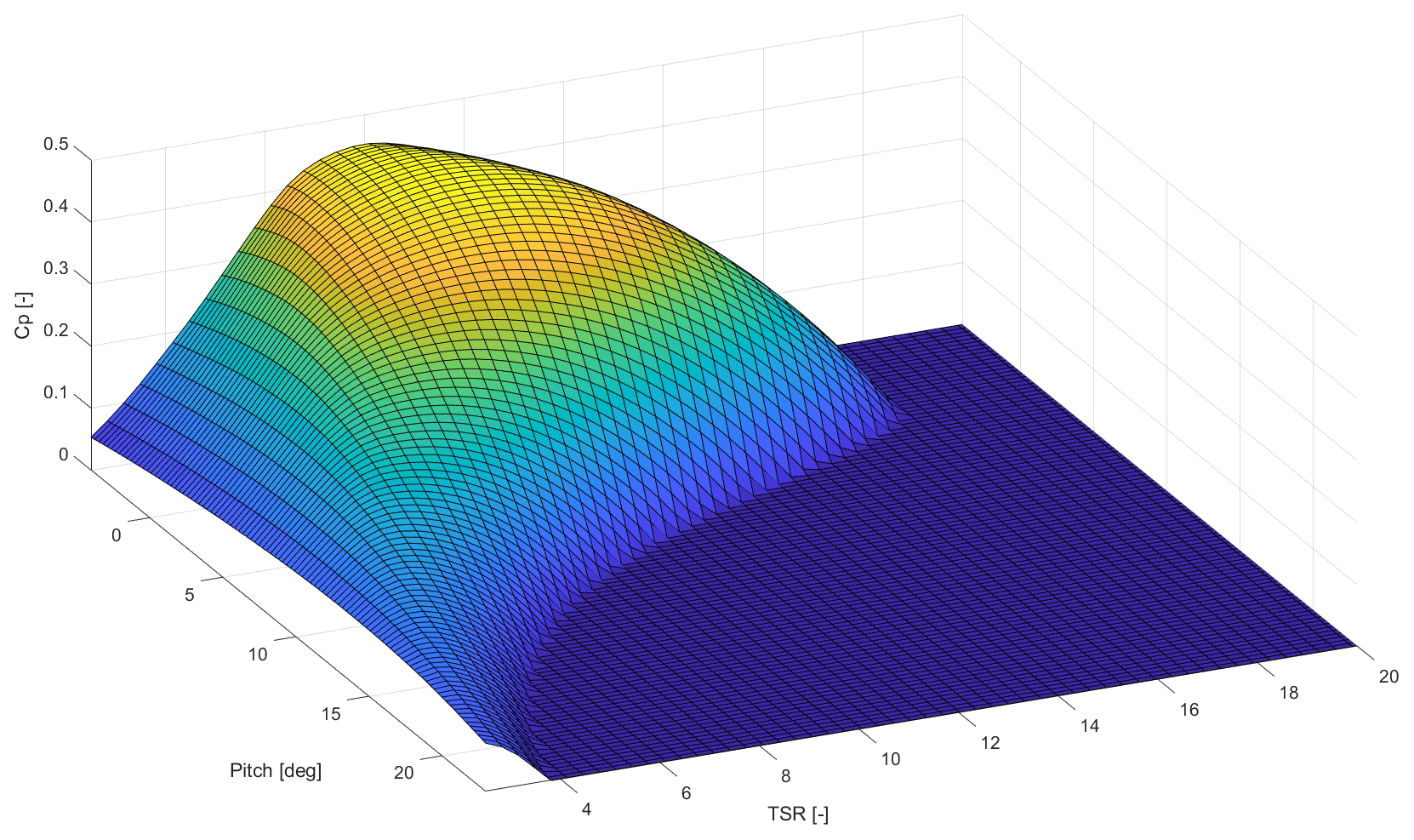
Figure A1Calculated Cp(β,λ) surface for the Vestas V52 turbine. For illustrative purposes, negative Cp values have been replaced with zero.
In this appendix, an example of the flow field around a rotor operating at the aerodynamic optimum according to the model of Conway (1995) is shown. The focus positions of the four-beam lidar are indicated in red.
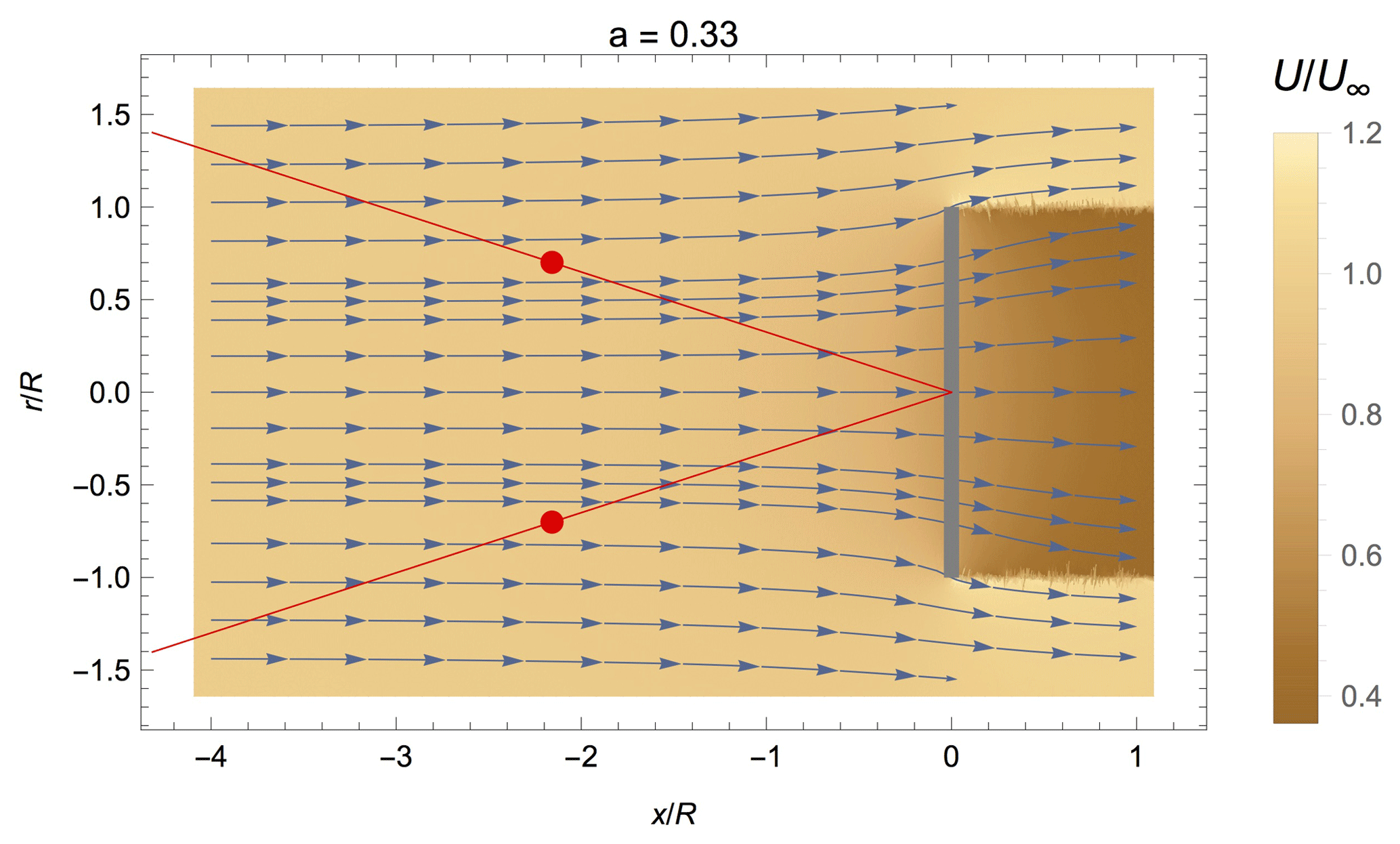
Figure B1Example of the flow speed reduction and diversion around the rotor of a wind turbine. The red lines indicate the laser beam and the red dots show the focus points.
In Sect. 3.2, the analysis was split into two distinct regions, of which region 1 was disturbed by buildings and vegetation, while region 2 had a more undisturbed inflow over field and the fjord. Previously, the average spectra were fitted to the Mann model for sectors of 30∘ width. The fitted parameter were then averaged per region to obtain a representative set of parameters for each region. Here, the averaged parameters are compared to the average spectra for regions 1 and 2. In the process, each individual u, v and w spectrum and the uw co-spectrum has been normalized by the 10 min mean wind speed squared, and the average over all spectra for each region was taken. The result can be seen for region 1 in Fig. C1a and for region 2 in Fig. C1b. It can be seen that in both cases the model is describing the u, v and w spectra well. The uw co-spectrum is underestimated by the model, which was also found in the fits done in Mann (1994).

DPH performed the research work and prepared the manuscript. JM conceived the research plan, supervised the research work and the manuscript preparation.
The authors declare that they have no conflict of interest.
This study was supported by Innovationsfonden Danmark in the form of an industrial PhD stipend. The authors also want to acknowledge the research project “Cost-efficient lidar for pitch control”, funded by Energiteknologiske Udviklings- og Demonstrationsprogram, and specifically Hector Villanueva for providing the turbine data in the form of a database, Qi Hu for designing and constructing the four-beam lidar, Ebba Dellwik for the coordination within the project and the technicians at DTU Wind Energy for conducting the experiments on the Vestas V52 turbine at the Risø test site. The authors also want to thank Pedro Santos and Ebba Dellwik for their comments and suggestions on the manuscript.
The work of Dominique P. Held was partly funded by Windar Photonics A/S in the form of an industrial PhD stipend (project no. 5016-00182).
This paper was edited by Carlo L. Bottasso and reviewed by three anonymous referees.
Agency for Data Supply and Efficiency: DHM/Terræn (0,4 m grid), available at: https://download.kortforsyningen.dk/content/dhmterr\%C3\%A6n-04-m-grid, last access: 6 December 2018. a
Batchelor, G. K.: The Theory of Homogeneous Turbulence, Cambridge University Press, 1953. a
Bossanyi, E.: Un-freezing the turbulence: application to LiDAR-assisted wind turbine control, IET Renew. Power Gener., 7, 321–329, 2013. a
Chougule, A., Mann, J., Segalini, A., and Dellwik, E.: Spectral tensor parameters for wind turbine load modeling from forested and agricultural landscapes, Wind Energy, 18, 469–481, 2015. a, b
Chougule, A. S., Mann, J., Kelly, M. C., and Larsen, G. C.: Simplification and Validation of a Spectral-Tensor Model for Turbulence Including Atmospheric Stability, Bound.-Lay. Meteorol., 167, 371–397, 2018. a
Conway, J. T.: Analytical solutions for the actuator disk with variable radial distribution of load, J. Fluid Mech., 297, 327–355, 1995. a, b
de Maré, M. and Mann, J.: Validation of the Mann spectral tensor for offshore wind conditions at different atmospheric stabilities, J. Phys. Conf. Ser., 524, 012106, https://doi.org/10.1088/1742-6596/524/1/012106, 2014. a
de Maré, M. and Mann, J.: On the Space-Time Structure of Sheared Turbulence, Bound.-Lay. Meteorol., 160, 453–474, 2016. a
Dunne, F., Pao, L. Y., Wright, A. D., Jonkman, B., and Kelley, N.: Adding feedforward blade pitch control to standard feedback controllers for load mitigation in wind turbines, Mechatronics, 21, 682–690, 2011. a, b
Dunne, F., Schlipf, D., Pao, L. Y., Wright, A., Jonkman, B., Kelley, N., and Simley, E. J.: Comparison of Two Independent Lidar-Based Pitch Control Designs, 50th AIAA Aerospace Sciences Meeting including the New Horizons Forum and Aerospace Exposition, Nashville, Tennessee, 9–12 January 2012, https://doi.org/10.2514/6.2012-1151, 2012. a
Dunne, F., Pao, L. Y., Schlipf, D., and Scholbrock, A. K.: Importance of lidar measurement timing accuracy for wind turbine control, Proc. Am. Control Conf., Portland, OR, USA, 4–6 June 2014, 3716–3721, https://doi.org/10.1109/ACC.2014.6859337, 2014. a
Haizmann, F., Schlipf, D., and Cheng, P. W.: Correlation-Model of Rotor-Effective Wind Shears and Wind Speed for Lidar-Based Individual Pitch Control, Proceedings of the 12th (2015) German Wind Energy Conference DEWEK, Bremen, Germany, 19–20 May 2015, 1–4, 2015a. a
Haizmann, F., Schlipf, D., Raach, S., Scholbrock, A. K., Wright, A. D., Slinger, C., Medley, J., Harris, M., Bossanyi, E. A., and Cheng, P. W.: Optimization of a feed-forward controller using a CW-lidar system on the CART3, Proceedings of the American Control Conference, Chicago, USA, July 2015, 3715–3720, 2015b. a
Harris, M., Hand, M., and Wright, A. D.: Lidar for turbine control, Tech. rep., NREL, 2006. a
Held, D. P. and Mann, J.: Comparison of methods to derive radial wind speed from a continuous-wave coherent lidar Doppler spectrum, Atmos. Meas. Tech., 11, 6339–6350, https://doi.org/10.5194/amt-11-6339-2018, 2018. a, b
Held, D. P., Kouris, N., and Larvol, A.: Wake detection in the turbine inflow using nacelle lidars, J. Phys. Conf. Ser., 1102, 012005, https://doi.org/10.1088/1742-6596/1102/1/012005, 2018. a
IEC: IEC 61400-1:2005 – Wind turbines Part 1: Design requirements, Tech. rep., IEC, 2005. a, b, c
Kaimal, J. C. and Finnigan, J. J.: Atmospheric Boundary Layer Flows, Their Structure and Measurement, Oxford University Press, New York, 1994. a
Kolmogorov, A. N.: The local structure of turbulence in incompressible viscous fluid for very large Reynolds numbers, Philos. T. R. Soc. S.-A, 434, 9–13, 1941. a
Kumar, A. A., Bossanyi, E. A., Scholbrock, A. K., Fleming, P. A., and Boquet, M.: Field Testing of LIDAR Assisted Feedforward Control Algorithms for Improved Speed Control and Fatigue Load Reduction on a 600 kW Wind Turbine, in: EWEA 2015 Annual Event, Paris, France, 17–20 November 2015. a
Laks, J. H., Pao, L. Y., Wright, A., Kelley, N., and Jonkman, B.: The use of preview wind measurements for blade pitch control, Mechatronics, 21, 668–681, 2011. a
Mann, J.: The spatial structure of neutral atmospheric surface-layer turbulence, J. Fluid Mech., 273, 141–168, 1994. a, b, c, d
Mann, J.: Wind field simulation, Probabilistic Eng. Mech., 13, 269–282, 1998. a
Mirzaei, M. and Mann, J.: Lidar configurations for wind turbine control, J. Phys. Conf. Ser., 753, 032019, https://doi.org/10.1088/1742-6596/753/3/032019, 2016. a, b, c, d
Mirzaei, M., Soltani, M., Poulsen, N. K., and Niemann, H. H.: Model Predictive Control of Wind Turbines using Uncertain LIDAR Measurements, P. Amer. Contr. Conf., Washington, DC, USA, 17–19 June 2013, https://doi.org/10.1109/ACC.2013.6580167, 2013. a
Mizuno, T. and Panofsky, H. A.: The Validity of Taylor'S Hypothesis the Atmospheric Surface Layer, Bound.-Lay. Meteorol., 9, 375–380, 1975. a
Moddemeijer, R.: An information theoretical delay estimator, Ninth Symposium on Information Theory in the Benelux, Mierlo, the Netherlands, 26–27 May 1988, 121–128, 1988. a
Monin, A. S. and Yaglom, A. M.: Statistical Fluid Mechanics, vol. 2, The MIT Press, 1975. a
Østergaard, K. Z., Brath, P., and Stoustrup, J.: Estimation of effective wind speed, J. Phys. Conf. Ser., 75, 012082, https://doi.org/10.1088/1742-6596/75/1/012082, 2007. a
Peña, A., Gryning, S.-E., Mann, J., and Hasager, C. B.: Length Scales of the Neutral Wind Profile over Homogeneous Terrain, J. Appl. Meteorol. Climatol., 49, 792–806, 2010. a
Sathe, A., Mann, J., Barlas, T., Bierbooms, W., and van Bussel, G.: Influence of atmospheric stability on wind turbine loads, Wind Energy, 16, 1013–1032, https://doi.org/10.1002/we.1528, 2012. a
Schlipf, D.: Lidar-Assisted Control Concepts for Wind Turbines, PhD thesis, University of Stuttgart, 2015. a, b
Schlipf, D. and Cheng, P. W.: Flatness-based Feedforward Control of Wind Turbines Using Lidar, IFAC Proc., 47, 5820–5825, 2014. a
Schlipf, D., Cheng, P. W., and Mann, J.: Model of the Correlation between Lidar Systems and Wind Turbines for Lidar-Assisted Control, J. Atmos. Ocean. Tech., 30, 2233–2240, 2013. a, b, c, d, e
Schlipf, D., Fleming, P. A., Haizmann, F., Scholbrock, A. K., Hofsäß, M., Wright, A. D., and Cheng, P. W.: Field Testing of Feedforward Collective Pitch Control on the CART2 Using a Nacelle-Based Lidar Scanner, J. Phys. Conf. Ser., 555, 12090, https://doi.org/10.1088/1742-6596/555/1/012090, 2014. a
Schlipf, D., Haizmann, F., Cosack, N., Siebers, T., and Cheng, P. W.: Detection of Wind Evolution and Lidar Trajectory Optimization for Lidar-Assisted Wind Turbine Control, Meteorol. Z., 24, 565–579, 2015. a
Schlipf, D., Fürst, H., Raach, S., and Haizmann, F.: Systems Engineering for Lidar-Assisted Control: A Sequential Approach, IOP Conf. Ser. J. Phys. Conf. Ser., 1102, 012014, https://doi.org/10.1088/1742-6596/1102/1/012014, 2018. a
Scholbrock, A. K., Fleming, P. A., Fingersh, L. J., Wright, A. D., Schlipf, D., Haizmann, F., and Belen, F.: Field Testing LIDAR-Based Feed-Forward Controls on the NREL Controls Advanced Research Turbine, 51st AIAA Aerospace Sciences Meeting, Grapevine, Texas, 7–10 January 2013, 1–8, 2013. a, b
Segalini, A. and Arnqvist, J.: A spectral model for stably stratified turbulence, J. Fluid Mech., 781, 330–352, 2015. a
Simley, E. J. and Pao, L. Y.: Reducing LIDAR wind speed measurement error with optimal filtering, 2013 American Control Conference, 621–627, https://doi.org/10.1109/ACC.2013.6579906, 2013a. a
Simley, E. J. and Pao, L. Y.: Correlation between Rotating LIDAR Measurements and Blade Effective Wind Speed, 51st AIAA Aerospace Sciences Meeting including the New Horizons Forum and Aerospace Exposition, Grapevine Texas, USA, https://doi.org/10.2514/6.2013-749, 2013b. a
Simley, E., Fürst, H., Haizmann, F., and Schlipf, D.: Optimizing lidars for wind turbine control applications – Results from the IEA Wind Task 32 workshop, Remote Sens., 10, 1–32, 2018. a
Soltani, M., Knudsen, T., Svenstrup, M., Wisniewski, R., Brath, P., Ortega, R., and Johnson, K.: Estimation of Rotor Effective Wind Speed: A Comparison, IEEE T. Contr. Syst. T., 21, 1155–1167, 2013. a
A lookup table of one-dimensional spectra obtained from the Mann model can be obtained from the second author at jmsq@dtu.dk
The adaptive cubature integration scheme was written by Steven G. Johnson and is available on GitHub: https://github.com/stevengj/cubature (last access: 6 August 2019).
The software can be downloaded free of charge at http://www.wasp.dk/weng\#details__iec-turbulence-simulator (last access: 6 August 2019).
- Abstract
- Introduction
- Methodology
- Experimental setup
- Results
- Conclusions
- Data availability
- Appendix A: Calculation of the power coefficient surface
- Appendix B: Induction correction
- Appendix C: Comparison between average fitted Mann model parameter and average spectra
- Author contributions
- Competing interests
- Acknowledgements
- Financial support
- Review statement
- References