Radar-derived precipitation climatology for wind turbine blade leading edge erosion

Wind turbine blade leading edge erosion (LEE) is a potentially significant source of revenue loss for wind farm operators. Thus, it is important to advance understanding of the underlying causes, to generate geospatial estimates of erosion potential to provide guidance in pre-deployment planning, and ultimately to advance methods to mitigate this effect and extend blade lifetimes. This study focuses on the second issue and presents a novel approach to characterizing the erosion potential across the contiguous USA based solely on publicly available data products from the National Weather Service dual-polarization radar. The approach is described in detail and illustrated using six locations distributed across parts of the USA that have substantial wind turbine deployments. Results from these locations demonstrate the high spatial variability in precipitation-induced erosion potential, illustrate the importance of low-probability high-impact events to cumulative annual total kinetic energy transfer and emphasize the importance of hail as a damage vector.

1 Introduction and objectives

In 2017 wind turbines (WTs) provided 6 % of total electricity generation in the United States of America (USA) (U.S. Energy Information Administration, 2018) and there are over 50 000 WTs operating in the USA today (Pryor et al., 2019). WTs are subject to harsh operating conditions during their 20–25-year lifetimes, including extreme winds, impacts from heavy rain, hailstones and snow, and intense ultraviolet light exposure that can lead to material damage (Keegan et al., 2013). Accordingly, operation and maintenance (O&M) costs comprise 20 %–25 % of the total levelized cost per kilowatt-hour of electricity produced over the WT lifetime (Mishnaevsky Jr., 2019; Moné et al., 2017). WT blades exhibit the highest failure rate (FR ∼0.2) of any WT component (Zhu and Li, 2018). The most expensive repair and longest repair times are associated with blades (Shohag et al., 2017). Estimates suggest that the average cost of blade repair of an onshore turbine is approximately USD 30 000, with replacement costs of ∼ USD 200 000 (Mishnaevsky Jr., 2019). Repair and replacement costs will tend to be higher offshore, where general O&M costs are higher (∼30 % of total cost) and blade failures also contribute significantly to turbine downtime (Carroll et al., 2016).

Hail has long been recognized as an important source of weather-related economic losses in the contiguous United States (CONUS) (Changnon, 1999; Cintineo et al., 2012). Economic losses from hail were estimated to be USD 1.2 billion in 1999 (Changnon, 1999), and property damage from severe hail has been shown to be increasing with time (Changnon, 2009), with more recent annual losses estimated at USD 10 billion, accounting for almost 70 % of severe-weather-related insurance claims (Loomis, 2018). An analysis conducted in 2009 indicated that an average of 159 d each year is associated with crop-damaging hail leading to average crop loss of USD 580 million, and hail damage to property was valued at USD 850 million (Changnon et al., 2009). Hail, and hail damage, are highly episodic. For example, insurance losses in the Dallas–Fort Worth (DFW) metroplex on a single hail day in May 2011 were estimated to exceed USD 876 million (Brown et al., 2015). While the paucity and subjectivity of observed hail data sets make a global comparison difficult, severe hail is almost certainly more common in the central US than in other areas of the world with substantial wind energy development (Prein and Holland, 2018). Further, the relationship linking damage to the frequency and severity of hail varies substantially with the target. WTs present an interesting challenge in this context because they are large structures and the blades are rotating, composite materials.

A key cause of the need for WT blade repairs is excess damage (i.e., material loss) on the leading edge (leading edge erosion, LEE). LEE roughens WT blades, reducing lift and electrical power production (Sareen et al., 2014; Gaudern, 2014). LEE causes an average of 1 %–5 % reduction in annual energy production (AEP) (Froese, 2018) and up to a 9 % reduction when delamination occurs (Schramm et al., 2017). Thus, excess LEE may be costing the industry tens of millions of dollars per year via lost revenue and/or increased maintenance costs and poses a threat to achieving continuing wind energy cost reductions (Sareen et al., 2014). In response to this issue a major industrial research consortium from Europe (including DNV GL, Vestas and Siemens Gamesa Renewable Energy) has recently (November 2018) announced a new partnership (COBRA) focused on the analysis of mitigation measures for LEE including the development of next-generation leading-edge protection systems (Durakovic, 2019).

WT blades use composites (e.g., epoxy or polyester, with reinforcing glass or carbon fibers) (Mishnaevsky Jr. et al., 2017) coated to protect the blade structure by distributing and absorbing the energy from impacts (Brøndsted et al., 2005). Thus, the leading edge actually comprises several layers of the main structural composite material (and thickening materials) plus coatings (Mishnaevsky Jr. et al., 2017). Impact fatigue caused by collision with rain droplets and hail stones is a primary cause of WT blade LEE (Bech et al., 2018; Bartolomé and Teuwen, 2019; Zhang et al., 2015). Although rain droplets fall at only modest velocities (typically ≤10 m s⁻¹, see details below), the tip of WT blades rotate quickly (50–110 m s⁻¹); thus the net closing velocity and kinetic energy transfer are large. Each precipitation impact on the blade leading edge results in transient stresses that are proportional to impact velocity (Preece, 1979; Slot et al., 2015). The stress induced by individual high net collision impacts with hydrometeors may, in principle, exceed the strength of the material. Estimates of the failure energy threshold of a composite structure vary widely (e.g., values of 72–140 J are given in Appleby-Thomas et al., 2011) and may exceed 300 J for leading-edge thicknesses and hailstone diameters >20 mm (Kim and Kedward, 2000). However, conceptually the erosion of homogeneous materials is most frequently considered using a three-stage model. Initially there is an incubation period during which impacts occur but no visible damage is observed, although microstructural changes in the materials generate nucleation sites for material removal, which commences when a threshold is reached (i.e., when some level of accumulated impacts is reached). Once the time to damage has been exceeded, additional damage occurs as stress waves propagate from the impact sites into the composite and cause existing pits and cracks to grow, and there is a steady increase of material loss with each additional impact (Cortés et al., 2017; Eisenberg et al., 2018; Traphan et al., 2018). The number of impacts required to reach the threshold for surface fatigue failure is a function of the droplet diameter and phase, the closing velocity, the strength of the material, and the pressure of the impact. Hence, the material's response to hail (solid hydrometeors) may differ from that to collisions with liquid (rain) droplets. For example, the maximum von Mises stress created in the WT blade leading edge from a 10 mm diameter hailstone greatly exceeds that from a rain droplet of equivalent size and closing velocity due to differences in mass and hardness (Keegan et al., 2013).

WT LEE is a developing area of research and uncertainty remains regarding the frequency and severity of the issue. Rates of LEE appear to be highly spatially variable due to variations in WT operating conditions and the precipitation climate. Industrial experience has demonstrated that exposure to particularly harsh operating conditions can erode coatings causing partial delamination after as little as 2–3 years (Rempel, 2012; Keegan et al., 2013). Elastomeric coatings can be applied for additional erosion resistance (Dalili et al., 2009; Valaker et al., 2015; Herring et al., 2019). However, the life of such coatings cannot be predicted accurately (and is a function of UV exposure; Shokrieh and Bayat, 2007); they have a negative impact on blade aerodynamics (Giguère and Selig, 1999) and their cost effectiveness is uncertain (Dashtkar et al., 2019).

The total installed capacity (IC) and rated capacity (and physical dimensions) of WT being installed exhibited marked growth in the USA over the last 20 years (Wiser and Bolinger, 2018; Wiser et al., 2016). Average WT blade length increased from <4 m in 1985 to 32 m in 2005 and now exceeds 55 m (Wiser and Bolinger, 2018). Since the tip speed increases with blade length, this tendency towards taller WTs with longer blades exacerbates LEE potential. The increased blade length and larger maintenance costs associated with offshore wind turbines tend to make offshore wind farms especially vulnerable to LEE. Based on previous research the a priori expectation of this research is that excess LEE is most likely on WTs deployed in environments with high rain intensities and hail frequencies, such as experienced in the Great Plains (the states of Texas, TX; Oklahoma, OK; Kansas, KS; Nebraska, NE; North and South Dakota, ND, SD; Wyoming, WY; and Montana, MN; Fig. 1). LEE is likely to present a growing issue within the US wind industry as more and larger wind turbines with higher tip-speed ratios are deployed (Amirzadeh et al., 2017a). The current average age of WTs in the US is 9 years (AWEA, 2019), and LEE will be of greater concern as a larger number of WTs move out of the typical 1- to 5-year warranty period (Bolinger and Wiser, 2012; Brown, 2010).

Addressing the challenges posed by blade LEE and developing mitigation options requires multi-scale and multidisciplinary research. Given the importance of precipitation phase, size and intensity during WT operation to the potential for blade LEE, here we focus on developing a consistent and generalizable framework that can be applied to derive estimates of erosion-relevant atmospheric properties. We present an objective, spatially consistent, robust and repeatable framework that can be applied across CONUS and crucially uses only noncommercial (i.e., publicly available) data. The specific objectives of the research reported herein are as follows:

• 1.

  to develop the workflow necessary to develop a prototype radar-based erosion atlas;

• 2.

  to provide a first estimate of the spatial variability of erosion potential across CONUS in regions where wind turbines are currently deployed (see Fig. 1);

• 3.

  to conduct an initial uncertainty propagation exercise to illustrate how uncertainties in the input data propagate through the analysis workflow to influence erosion potential estimates;

• 4.

  to describe the degree to which blade LEE is episodic and therefore amendable to the mitigation strategy proposed earlier in research from Denmark of WT curtailment during “highly erosive” periods. The efficacy of this strategy is a function of (i) the wind speed regime and joint probability distributions of erosive events (heavy rain or hail) and power-producing wind speeds, (ii) the price of electricity supplied to the grid and (iii) O&M costs. A cost–benefit analysis based on conditions in Denmark suggested that the loss of revenue from the curtailment of power production was small compared to the economic benefits from enhanced blade lifetimes (Bech et al., 2018).

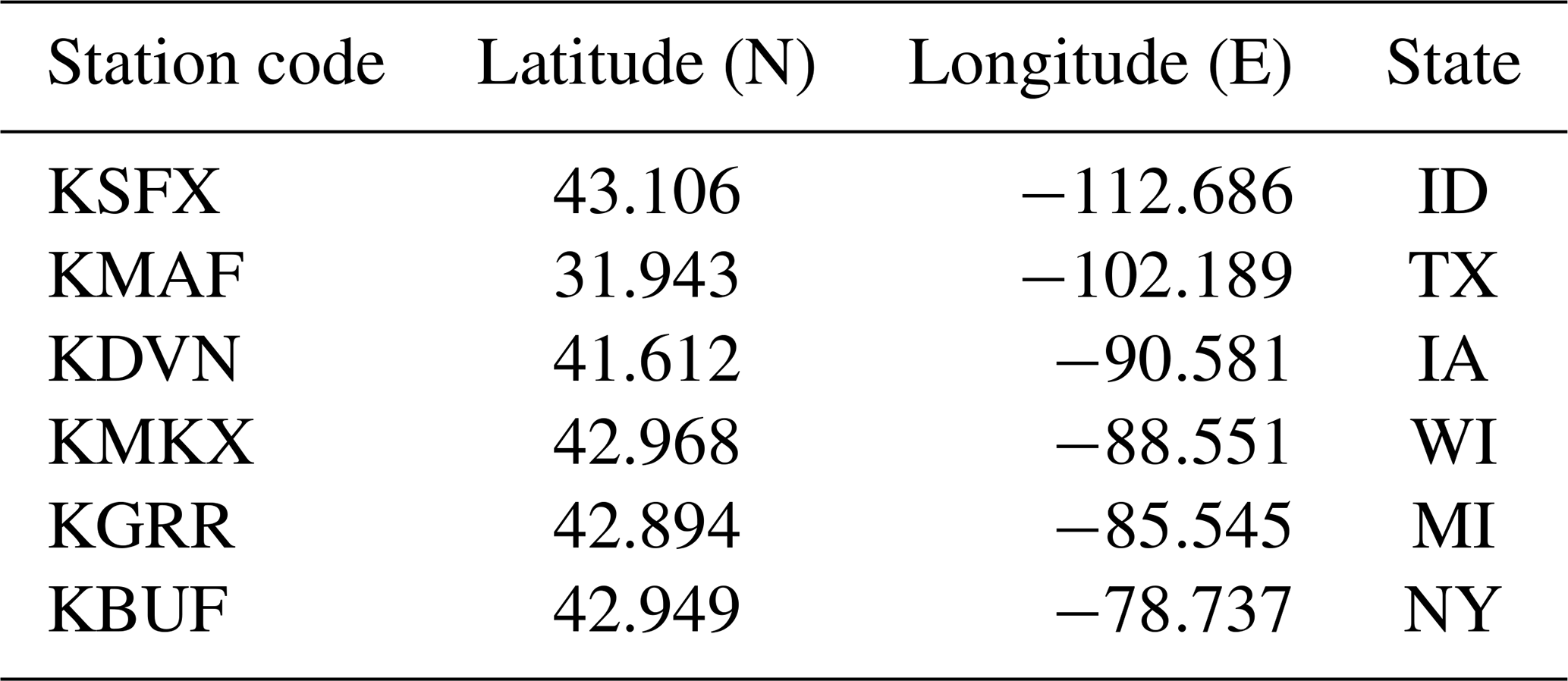
Figure 1 Locations of wind turbines as deployed at the end of 2017 according the USGS database (available from https://eerscmap.usgs.gov/uswtdb/, last access: 15 January 2020; USGS, 2018) (grey dots), the NWS radar stations from which data are presented (see details in Table 1) and areas of frequent hail occurrence. Areas with more than 9 hail days per year are outlined by the red contour, and those with more than six are outlined by the blue contours (Cintineo et al., 2012).

Table 1 The station code and locations of the six NWS dual-polarization radars from which data are presented (listed from west to east).

2 Data and methods

A first estimate of precipitation-derived erosion potential at sites across the USA as developed in the current work is based on a characterization of the kinetic energy exchange from rain and hail impacts on the blade leading edge. The procedure used in making these estimates is divided into two steps: the calculation of meteorological parameters (wind speed, rain and hail) at six wind farms, each located within the observation area of a radar station, and then the calculation of blade impact frequencies and energy transfer based on those meteorological parameters. Exact wind farm locations and details are excluded from this paper under a nondisclosure agreement (NDA).

The research reported herein leverages resources generated from the upgraded National Weather Service (NWS) network of WSR-88D radar to dual polarization (completed in 2013; Seo et al., 2015; Crum et al., 1998) along with the NOAA Weather and Climate Toolkit (WCT) (see details of the data products and data volumes provided in Appendix A). These data represent a unique opportunity to characterize precipitation properties such as hail that are very challenging to detect and to accurately characterize using in situ methods or human observers (see discussion in Allen and Tippett, 2015, and details of radar operation in Kumjian, 2018). NWS radars operate at elevation angles between 0.5 and 19.5^∘ and an azimuthal resolution of 1^∘. Doppler and dual-polarization data are publicly available at a resolution of 0.25 km up to a range of 300 km from each radar site (NOAA, 1991; Istok et al., 2009) (see description of the data provision in Kelleher et al., 2007, and an example of the NWS products given in Fig. 2). The temporal resolution of the data is typically ∼5 min, but varies slightly with scanning mode: (1) clear-air mode uses longer, 10 min scans to collect sufficient return data during times of no precipitation when signal return strength is relatively low; (2) precipitation mode is used when there is any precipitation detected in the scan area and uses a 6 min scan cycle; (3) storm mode is used when severe or rapidly evolving storms are present and uses a 5 min sampling interval, made possible by reducing the number of elevation angles used (NOAA, 2016a). Storm detection and tracking using radar is a complex and evolving science, but in brief the NWS system uses an automated function which employs reflectivity from the current scan and storm cell location and vertically integrated liquid water (VIL) from the previous scan (Johnson et al., 1998).

To illustrate the proposed analysis framework we use data from six NWS dual-polarization Doppler radar stations (see Fig. 1 and Table 1) collected over the period 2014–2018. These locations were chosen to represent gradients in hail probability and precipitation amount in regions with relatively high wind turbine installed densities (Fig. 1). We employ the framework in order to generate erosion climates for six wind farms operating in the scanned volume of the radars and located 35–75 km from the radar locations. The following radar data products are used (see also Appendix A):

• Precipitation rate (N1P) is the precipitation rate in each radar cell in each ∼5 min period (expressed in units of millimeters per hour) as estimated from reflectivity.

• Hybrid Hydrometer Classification (HHC), based on reflectivity, temperature and dual-polarization variables, is an estimate of the most likely targets within the radar volume. While this is a derived product, classification algorithms and accuracy have improved with the widespread adoption of dual-polarization radar and the application of areal (rather than point-wise) techniques (NOAA, 2016b; Chandrasekar et al., 2013). The hydrometeor types encoded in the NWS data product are dry snow, wet snow, crystals, big drops, rain (light and moderate), heavy rain, graupel and rain with hail.

• In hail reports (NHI), maximum hail size (an estimate of the 75th percentile hail stone diameter, D₇₅) and the probability of hail are used to identify the occurrence and severity of hail events (see discussion in Witt et al., 1998).

• Composite reflectivity (NCR) is the maximum reflectivity at any elevation angle measured in each radar cell. This is used here to characterize the spatial extent of hail events (i.e., reflectivity >50 dBZ (decibel reflectivity), Witt et al., 1998).

• Radial wind speeds from the 0.5 elevation angle are computed from the Doppler shift (N0V) (Alpert and Kumar, 2007).

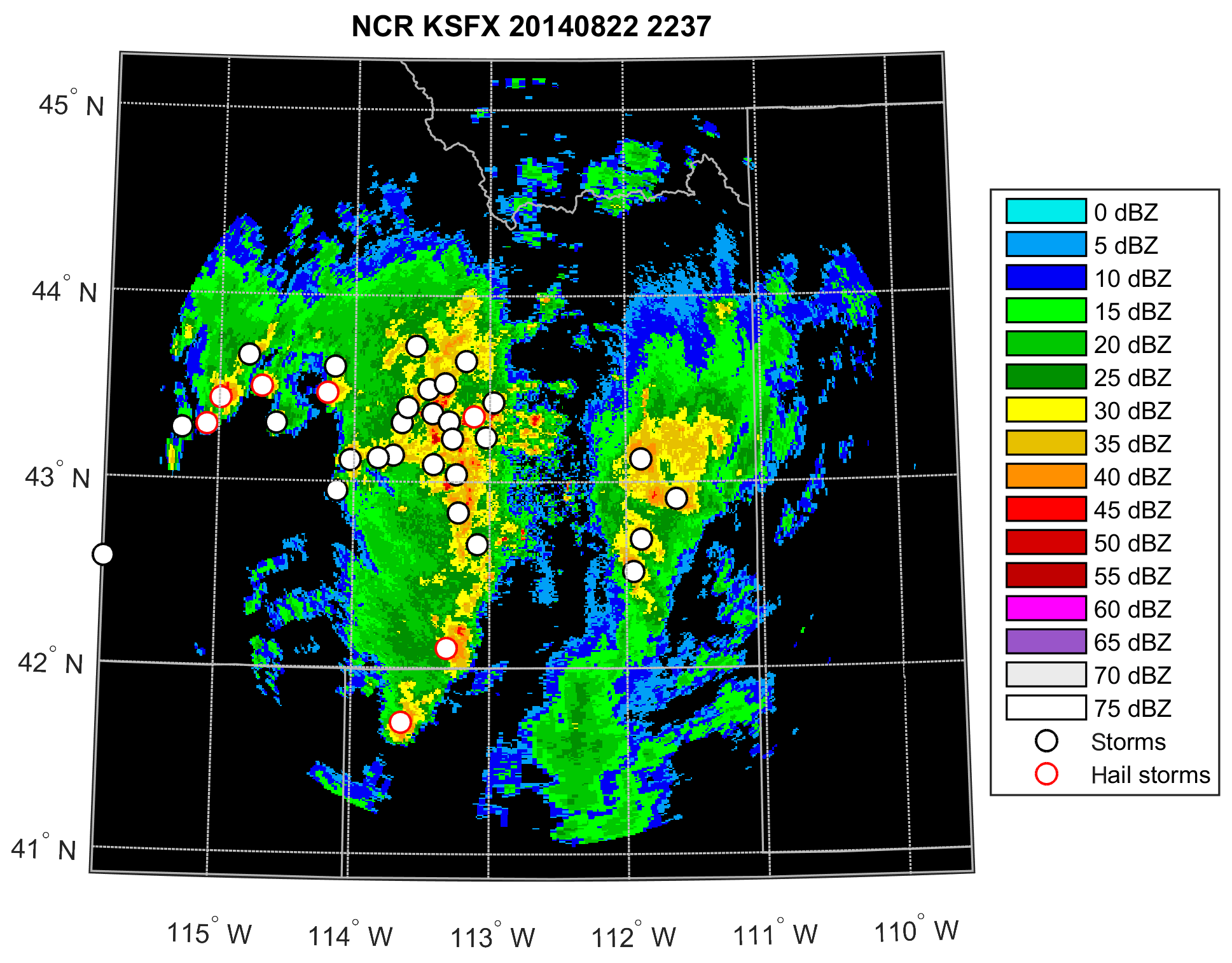
Figure 2 Example of a single 5 min period of radar data from KSFX (ID; 8 August 2013, 22:37 UTC). The colors show the composite reflectivity (i.e., the maximum reflectivity from any of the elevation angles sampled by the NWS radar) in decibel reflectivity (dBZ). The circles represent storm cells that are identified and tracked by the NWS detection algorithm; black circles are storms without hail, and red circles are those with hail.

Wind speeds, hydrometeor type and precipitation intensity for each nominal wind farm located within each radar-scanned area in each 5 min period are derived as follows.

Precipitation intensity is characterized by rainfall rate (RR) in millimeters per hour, which is derived using radar Z–R relationships (Wilson and Brandes, 1979) and reported in the parameter precipitation rates (N1P) in all radar cells every ∼5 min. A spatial mean of all N1P values in all radar cells within 5 km of the wind farm centroid is used here. This rainfall rate is also used to derive the raindrop spectrum using the Marshall–Palmer distribution (Marshall and Palmer, 1948). In it the number of droplets above radius, R, per cubic meter of air (N, m⁻³) is given by

$$\begin{array}{}\text{(1)}& N={\displaystyle \frac{N_{\mathrm{0}}}{\mathrm{\Lambda }}}{e}^{-\mathrm{\Lambda }R},\end{array}$$

where Λ=8200 (RR)^−0.21 (m⁻¹), RR is the rainfall rate in millimeters per hour and $N_{\mathrm{0}}=\mathrm{1.6}\times {\mathrm{10}}^{\mathrm{7}}$ m⁻⁴; see an example rain droplet size distribution, expressed as dN∕dR, for an RR of 25 mm h⁻¹ in Fig. 3.

Hail occurrence is characterized by a number of NWS radar-derived parameters, most of which are contained in the hail reports (NHI). Hail size and the probability of occurrence are conservatively estimated here, by taking the largest D₇₅ value and hail probability reported for any storm cell within 5 km of the nominal wind farm centroid (which will tend to bias both toward higher values). The spatial coverage of hail within that 5 km radius is determined by calculating the fraction of radar cells in that area which have a composite reflectivity in excess of 50 dBZ. Hail size distributions are relatively uncertain but are generally considered to be exponential up to a ceiling diameter (Auer, 1972; Lane et al., 2008). Herein the size distribution of hailstones is assumed to follow (Cheng and English, 1983)

$$\begin{array}{}\text{(2)}& N\left(D\right)=\mathrm{115}{\mathit{\lambda }}^{\mathrm{3.63}}{e}^{-\mathit{\lambda }D},\end{array}$$

where D is the hailstone diameter (Cheng and English, 1983). This formulation is based on seven events sampled in Alberta, Canada, which covered a smaller diameter range than indicated by the radar products, but it has the advantage that the distribution requires a single fitting parameter (λ) and thus can be fully described using only D₇₅. As shown by the example hail distribution (expressed in dN∕dR) for D₇₅=25 mm and λ=0.053 mm⁻¹ (Fig. 3), the slope of the hydrometeor diameter is considerably shallower than for rain droplets as described using Marshall–Palmer. In order to avoid the occurrence of extremely large hailstones, we truncate the distribution to include diameters up to 2 times the radar-estimated 75th percentile hail stone diameter (D₇₅). The presence of such a hail size ceiling is consistent with previous observations (Auer, 1972).

Wind speeds from radar have been previously used for numerical wind resource verification (Salonen et al., 2011). Wind speeds at a typical wind turbine hub height of approximately 80 m are derived using the radial wind speeds from the 0.5^∘ elevation angle scan at a distance of 8 km (±0.5 km) range from the radar station using an assumption of uniform flow from

$$\begin{array}{}\text{(3)}& V_{\mathrm{radial}}\left(\mathit{\theta }\right)=V_{\mathrm{mean}}\cos \left(\mathit{\theta }\right),\end{array}$$

where θ is the difference in angle between the radar beam and the direction of mean flow and V_mean is the mean wind speed at hub height. A least-squares fit of a sinusoid of this form is made to each wind speed scan (excluding cells which report a zero wind speed) to estimate V_mean. The resulting wind speed is then used within the simple description of the blade rotational speed as a function of hub-height wind speed as shown in Fig 4c. This operational RPM (revolutions per minute) curve is based on long-term data provided from large operating WT arrays (under an NDA) and represents the mean rotational speed across all WTs operating in these arrays as a function of the mean wind speed at hub height across the arrays. The mean RPM decreases at wind speeds below the cut-out velocity (of 25 m s⁻¹) due to some WTs rotating below their design RPM at very high wind speeds (near cut out) as reported in the SCADA (supervisory control and data acquisition) data.

Once the hydrometeor type (rain or hail), hydrometeor size (which determines mass and terminal velocity) and wind speed for a reporting period are known, hydrometeor impact energies for that period are calculated using the mass and closing velocity for hydrometeors of each radius occurring in the period. For this analysis the terminal velocity for each size of rain droplets is derived using (Stull, 2015)

$$\begin{array}{}\text{(4)}& V_{\mathrm{t},\mathrm{rain}}=k{\left[{\displaystyle \frac{{\mathit{\rho }}_{\mathrm{0}}}{{\mathit{\rho }}_{\mathrm{air}}}}R\right]}^{\mathrm{1}/\mathrm{2}},\end{array}$$

where R is the droplet radius (m), k=220 m^1∕2 s⁻¹ and ρ₀ is air density at sea level (set to a constant of 1.25 kg m⁻³, herein), ρ_air is air density at the altitude above sea level at which the rain droplet is crossing the rotor plane (see example of V_t, rain in Fig. 3). The terminal velocity of hail stones is derived using (Stull, 2015)

$$\begin{array}{}\text{(5)}& V_{\mathrm{t},\mathrm{hail}}={\left[{\displaystyle \frac{\mathrm{8}}{\mathrm{3}}}{\displaystyle \frac{\left|g\right|}{C_{\mathrm{D}}}}{\displaystyle \frac{{\mathit{\rho }}_{\mathrm{i}}}{{\mathit{\rho }}_{\mathrm{air}}}}R\right]}^{\mathrm{1}/\mathrm{2}},\end{array}$$

where R is radius of the hailstone (m), ρ_i is the density of ice (set to a constant of 900 kg m⁻³ herein) and ρ_air is air density at the altitude at which the hail is falling. C_D=0.55 is the drag coefficient (Stull, 2015) (see example of V_t, hail in Fig. 3).

Closing velocity, V_c, as a function of hydrometeor type and diameter (D) is calculated from wind speed, V_mean, rotor speed, V_r (calculated from wind speed and RPM curve), terminal velocity, V_t, and blade position, ϕ(t). V_r as derived here represents the linear speed of the blade tip due to rotation, as this will lead to conservative estimates of impact energy. Local blade speeds increase linearly with distance from the hub, so both the frequency and the energy of impacts is at a maximum near the blade tip, where blades are particularly susceptible to erosion (Keegan et al., 2013).

$$\begin{array}{}\text{(6)}& V_{\mathrm{c}}\left(D,t\right)={\left[V_{\mathrm{mean}}^{\mathrm{2}}+{\left(V_{\mathrm{r}}+V_{\mathrm{t}}\left(D\right)\cdot \cos \left(\mathit{\varphi }\left(t\right)\right)\right)}^{\mathrm{2}}\right]}^{\mathrm{1}/\mathrm{2}}.\end{array}$$

The impact rate (I) on the blade leading edge as a function of hydrometeor type and size is calculated from the number density of the hydrometeors of a given diameter (N(D)) and the closing velocity:

$$\begin{array}{}\text{(7)}& I\left(D,t\right)=N\left(D\right)\cdot V_{\mathrm{c}}\left(D,t\right).\end{array}$$

The assumption that all falling rain droplets will impact the blade is made on the basis of evidence that only droplets with diameters below 0.2 mm have insufficient inertia to be deflected from the blade by streamline deformation (Eisenberg et al., 2018). The maximum kinetic energy transferred to the blade from the hydrometeors is then computed for each hydrometeor type and diameter using the following approximation:

$$\begin{array}{}\text{(8)}& E_{\mathrm{K}}\left(D,t\right)={\displaystyle \frac{\mathrm{1}}{\mathrm{2}}}m\left(D\right)\cdot V_{\mathrm{c}}{\left(D,t\right)}^{\mathrm{2}},\end{array}$$

where m(D) is the mass of the hydrometeors of a given diameter.

The total kinetic energy of impacts over a time interval, T, associated with hydrometeors of diameter, D, is given by:

$$\begin{array}{}\text{(9)}& E_{\mathrm{K},T}\left(D\right)={\int }_{t_{\mathrm{0}}}^{t_{\mathrm{0}}+T}I\left(D,t\right)\cdot E_{\mathrm{K}}\left(D,t\right)\mathrm{d}t,\end{array}$$

where dt is the time interval at which the radar measurements are available (5 min).

The radar-estimated probability of hail and the geographic extent of hail fall are both treated probabilistically with respect to the number of expected hail impacts on any particular wind turbine within the wind farm. The number of expected impacts at each kinetic energy are multiplied by two factors representing two effects: (1) the probability of hail being associated with the storm in question, as estimated by the radar hail detection algorithm, and (2) the fraction of radar cells within 5 km of the wind farm centroid which have a composite reflectivity of >50 dBZ, the range commonly associated with hail.

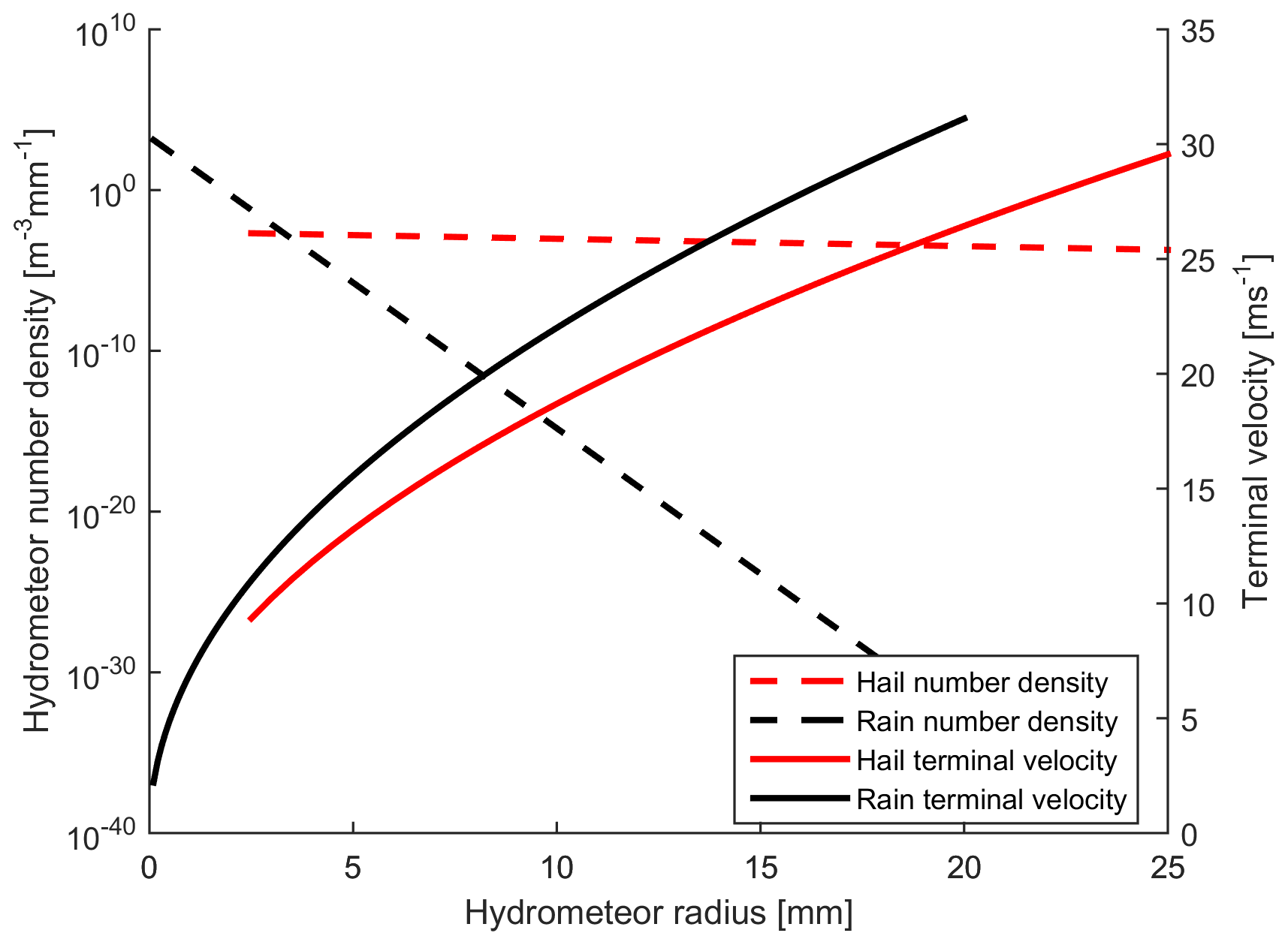
Figure 3 Example of the hydrometeor number density (dN∕dR; number of droplets per meter cubed of air per millimeter of radius increment) for a precipitation rate of 25 mm h⁻¹ for rain droplets (as described using the Marshall–Palmer size distribution) and for hail stones (for D₇₅ of 25 mm and λ=0.053 mm⁻¹) (left axis). Note: the λ value employed (λ=0.053 mm⁻¹) differs from the range (λ: 0.1 to 2 mm⁻¹) used by Cheng and English (1983) for the seven events they sampled and thus corresponds to a larger maximum hail size. Hydrometeor terminal velocities of hail and rain are shown by radius on the right axis.

NWS radar products have been subject to extensive product development efforts and a wide range of evaluation exercises (Cunha et al., 2015; Villarini and Krajewski, 2010; Straka et al., 2000) but are nevertheless associated with measurement uncertainties, as are the approximations applied herein to derive terminal fall velocities and kinetic energy transfer. To provide a first assessment of how these uncertainties in input data propagate through the analysis framework and thus impact derived kinetic energy exchange, each of three key parameters of the erosion potential are perturbed from 50 % to 150 % of observed values during two example periods of comparatively high erosion potential. The first case represents a period of large hail. In this analysis D₇₅ is set to the 99th percentile D₇₅ at KMKX (WI) (42 mm) and V_mean is set to 11.3 m s⁻¹ (i.e., the mean wind speed conditionally sampled by ±10 % of D₇₅=42 mm). In the second, a heavy rain event is considered. The RR is set to the 99th percentile value at KMKX (18 mm h⁻¹) and the V_mean is set to the mean value (12.8 m s⁻¹) during heavy rainfall (i.e., RR within 10 % of the 99th percentile value at KMKX).

Uncertainties in radar-derived hail sizes are less well characterized than for V_mean and RR. For RR the range of ±50 % is inclusive of previously published uncertainties, understanding that those uncertainties are a function of spatial resolution, RR and the radar processing algorithm (Seo and Krajewski, 2010; Seo et al., 2015). Wind speed uncertainty (as quantified using RMSE) for an elevation angle of 0.5^∘ is approximately ±3.4 m s⁻¹ (Fast et al., 2008), and thus for a wind speed of 12.8 m s⁻¹ a ±50 % variation is fully inclusive of the estimated wind speed error.

3 Results

Key aspects of the erosion-relevant radar-derived atmospheric properties at the six locations are summarized in Fig. 4. Consistent with previous precipitation climatologies, there are marked spatial gradients in the annual total and precipitation intensity (RR, Fig. 4a) (Prat and Nelson, 2015). Precipitation rates of <5 mm h⁻¹ are common at all sites; RRs of 20 mm h⁻¹ are experienced at all locations, but only the site in Texas (KMAF) exhibits any occurrence of rainfall intensity in excess of 35 mm h⁻¹. Using a damage rate of $\mathrm{3}\times {\mathrm{10}}^{-\mathrm{5}}$ s⁻¹ for an RR of 20 mm h⁻¹ and a closing velocity of 120 m s⁻¹ (Eisenberg et al., 2018), the frequency of RR of 20 mm h⁻¹ at the site in Texas is such that it would accumulate ∼0.6 of impact necessary to reach the transition threshold from the incubation region to material loss over a 25-year period.

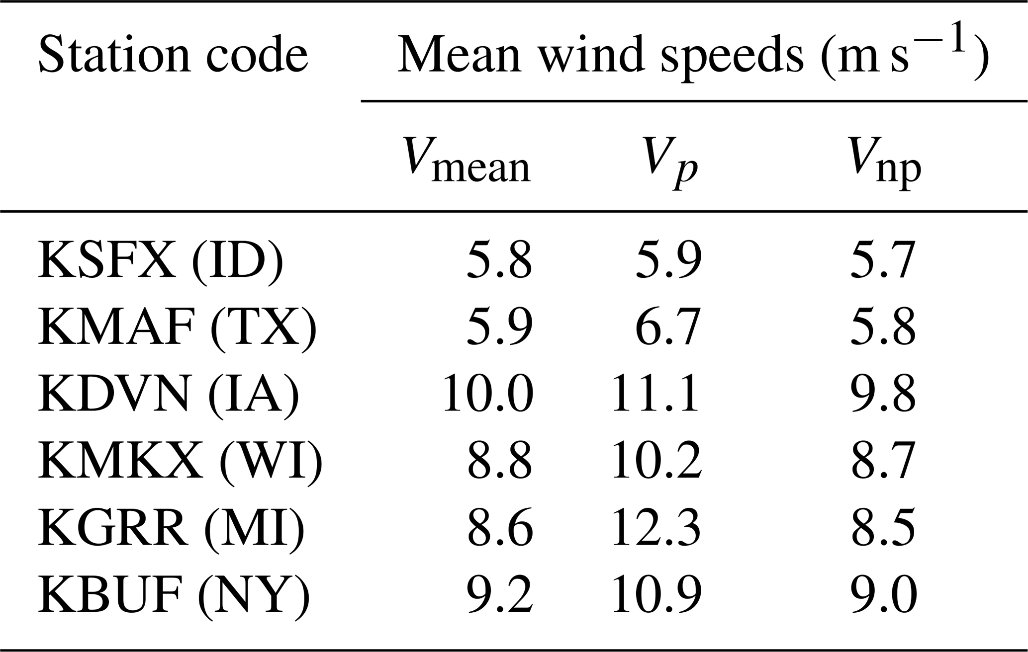
At most sites, snow and ice occur at rates at least 1 order of magnitude less frequent than rain. The exception is the site in Idaho (KSFX) (Fig. 4d). At each of the six locations, there are fewer than forty 5 min hail periods per year. Consistent with expectations and previous research (Cintineo et al., 2012), while hail events occur at all six sites, hail frequency and severe hail events (with maximum hail sizes >25 mm) are substantially more frequent at the nominal wind farm locations in Texas, Illinois and Wisconsin (radar codes: KMAF, KDVN and KMKX) (Fig. 4b). The derived frequency distributions of wind speed close to wind turbine hub heights (WT HHs) exhibit a high frequency of wind speeds above typical wind turbine cut-in speeds and are particularly right-skewed at the site in Iowa (Fig. 4c). The mean annual wind speed near nominal WT HH is lowest at KSFX (ID), where it is ≈5.9 m s⁻¹. Wind speeds range from 8.6 to 10 m s⁻¹ at KGRR (MI), KMKX (WI), KBUF (NY) and KDVN (IA) (Table 2). The wind speed distributions at these five of the six locations exhibit relatively good qualitative agreement with a priori expectations (see wind resource maps available at https://windexchange.energy.gov/maps-data/324, last access: 15 January 2020) and estimates from simulations for 2002–2016 with the Weather Research and Forecasting model (Pryor et al., 2018) for 12 km grid cells containing the nominal wind field locations that indicate mean annual wind speeds of 6.5 m s⁻¹ at KSFX (ID) and 8.4–9.0 m s⁻¹ (KGRR (MI), KMKX (WI), KBUF (NY) and KDVN (IA)). However, wind speeds derived from radar observations from KMAF (TX) are relatively low (mean value of 5.9 m s⁻¹) and exhibit a relatively low frequency of observations above 13 m s⁻¹ (2.2 %). This negative bias (of >1 m s⁻¹ in the mean relative to the resource map and WRF model output) from the Texas site will tend to lead to lower RPM values and hence blade tip speeds and thus a negative bias in kinetic energy transfer at this location. Wind speed distributions during precipitation and no-precipitation periods are qualitatively similar at all six locations. Modal values are within ±1.2 m s⁻¹, but the distributions are heavier-tailed at all sites during precipitation periods. Mean wind speeds during precipitation are 0.2–3.8 m s⁻¹ higher at the six locations than during times of no precipitation (Table 2).

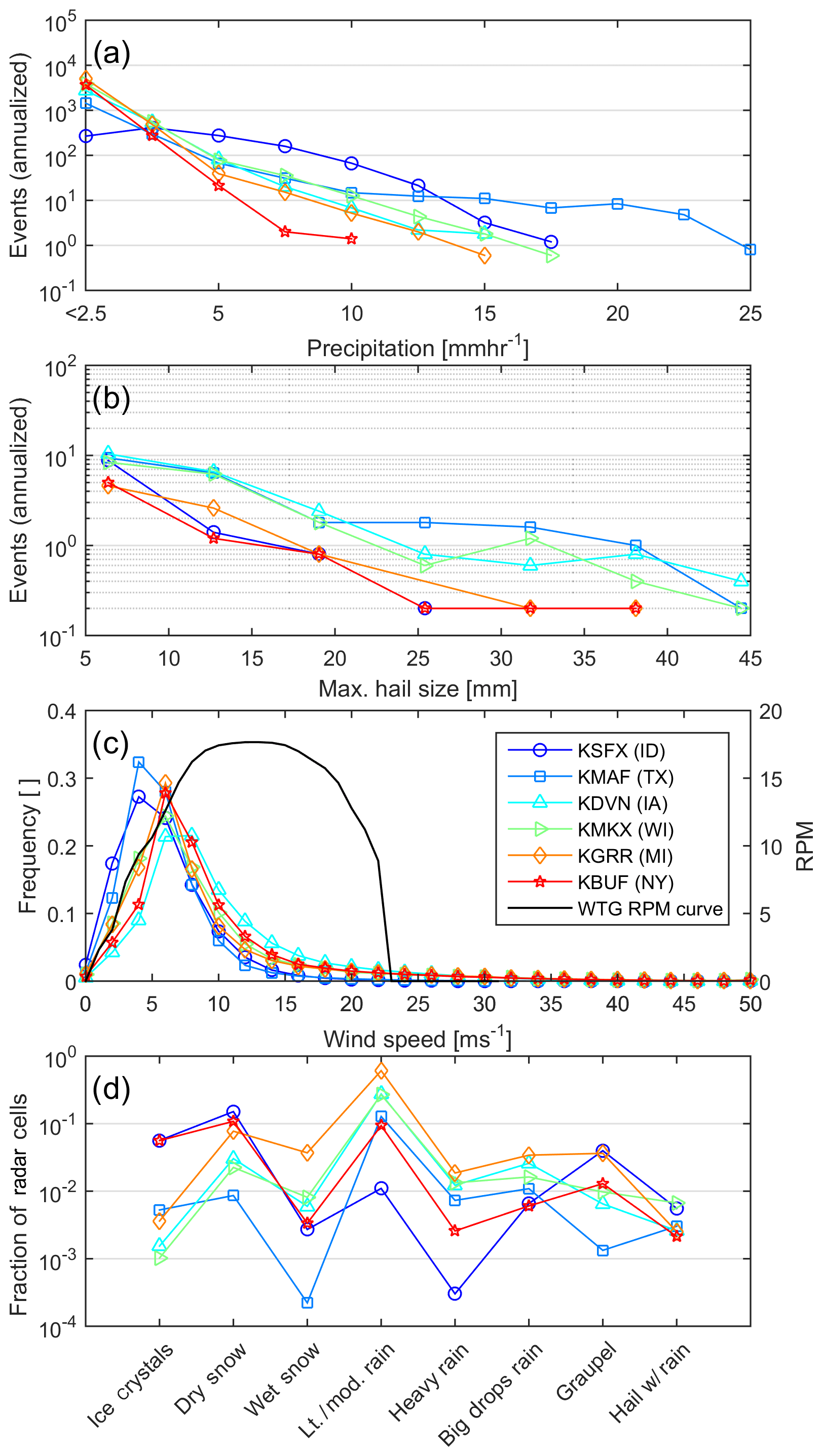
Figure 4 Precipitation and wind speed climates from radar data (see locations in Fig. 1). (a) Mean annual number of 5 min periods of each RR intensity class (discretized in 5 mm h⁻¹ intervals). (b) Mean annual number of 5 min periods with maximum hail sizes (D₇₅) (discretized in 5 mm intervals). (c) Wind speed distributions for all 5 min periods (discretized in 2 m s⁻¹ intervals). The black line in this frame shows the WT RPM curve as a function of wind speed (WTG RPM, right axis) (d). Occurrence of NWS radar hydrometeor classifications for each nominal wind farm shown as the fraction of radar cells in each class during all periods with RR>1 mm h⁻¹.

Table 2 Mean wind speeds close to WT HH from each radar: the long-term mean, V_mean, the mean during times of precipitation, V_p, and the mean during times of no precipitation V_np.

Given the exponential dependence of hailstone and rain droplet size on precipitation intensity and the accumulated damage therefrom (Eisenberg et al., 2018), the distributions of kinetic energy transfer from the two hydrometeor types at all sites are heavy-tailed. Further, the probability distributions of each 5 min estimate of kinetic energy transfer (Fig. 5) and total annual kinetic energy transfer (Fig. 6) indicate marked differences between the sites and between the two hydrometeor types. Extremely high hail kinetic energies are most frequently projected for sites in Texas (KMAF), Iowa (KDVN) and Wisconsin (KMKX) (Fig. 5a). This is consistent with the precipitation climatology summarized in Fig. 4b and the high frequency of wind speeds associated with high WT RPM (Fig. 4c). At these three sites some events (5 min periods) exhibit kinetic energy of transfer from hail in excess of 300 J (Fig. 5a). Although these events have a low probability (less than 1 m⁻² yr⁻¹), they may thus be sufficient to cause damage to blade coatings in isolation from the effects of the cumulative fatigue (Appleby-Thomas et al., 2011; Kim and Kedward, 2000). Conversely, individual rain impacts rarely exceed 5.2 J at any site. The probability of exceeding this impact kinetic energy threshold over a square meter of blade leading edge is less that 10⁻³ yr⁻¹ (Fig. 5b). Thus, hail dominates the annualized cumulative kinetic energy of transfer to each square meter of the blades at all sites (Fig. 6). Indeed, at all sites, despite the low probability of hail relative to rain (cf. Fig. 4a and b), total annual kinetic energy transfer from hail exceeds that from rain by at least 2 orders of magnitude (Fig. 6). The lowest cumulative kinetic energy transfer is projected for the nominal wind farm sites in Idaho (KSFX), New York state (KBUF) and Michigan (KGRR). Conversely, values are highest for Texas (KMAF), Iowa (KDVN) and Wisconsin (KMKX). This is consistent with previous characterizations of hail frequency, which show hail fall to be most common in the Great Plains and much less frequent west of 105^∘ W (Fig. 1) (Cintineo et al., 2012; Allen and Tippett, 2015).

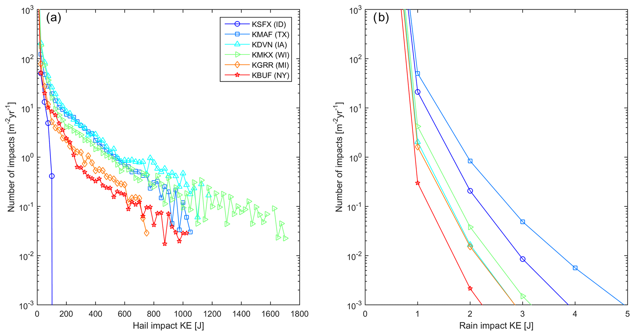
Figure 5 Histograms of kinetic energy of hydrometeor impacts. Annual number of (a) hail and (b) rain impacts per square meter of blade leading edge as a function of impact kinetic energy. The y axis in panel (b) has been truncated to a maximum value of 1000 yr⁻¹.

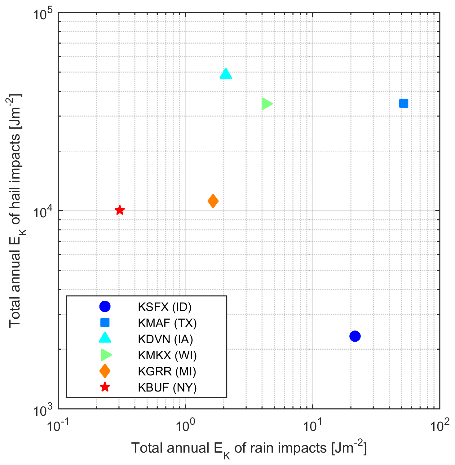
Figure 6 Total annual kinetic energy (E_K) per square meter of blade leading edge from rain and hail impacts at each location.

Figure 7 illustrates that only a very small fraction of 5 min periods dominate kinetic energy transfer to the blades from both hail and rain. At all sites over 80 % of rain-induced kinetic energy transfer occurs in the top eighty 5 min periods per year. Indeed, at all but the site in Idaho (KSFX) over half of the total rain-induced kinetic energy transfer to the blade occurs in only twenty 5 min periods in a year. The probability distribution of hail-induced kinetic energy transfer is even more heavy-tailed with 90 % of the cumulative kinetic energy transfer to the blades from hail occurring in fewer than twenty-five 5 min periods per year at all sites. Thus, few events dominate the annual total accumulated impact damage.

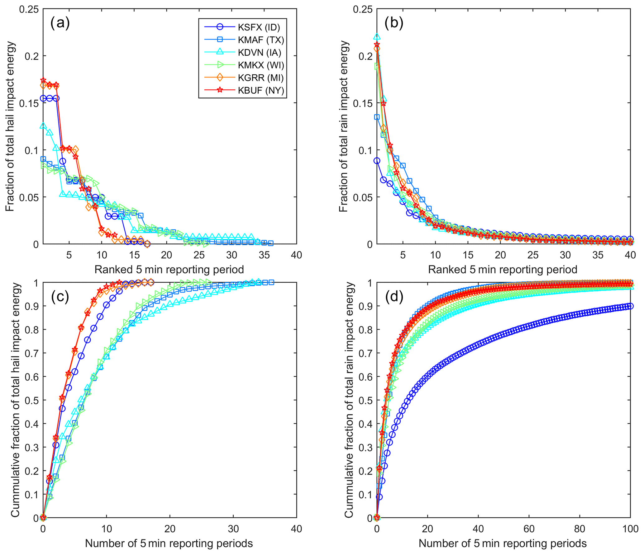
Figure 7 Contributions of the most intense precipitation events to annual total kinetic energy from hydrometeor impacts. (a) Contribution of the top forty 5 min periods of hail as a fraction of the annual total kinetic energy of hail impacts. (b) Contribution of the top forty 5 min periods of rain as a fraction of the annual total kinetic energy of rain impacts. Cumulative fraction of annual impact kinetic energy from the top X (c) hail events and (d) rain events, where X is set to 40 for hail because no site exhibits more than 36 events per year and is truncated to 100 for rain.

Illustrative examples of uncertainties in impact kinetic energy due to radar observational uncertainties in V_mean, RR and D₇₅ are shown in Fig. 8. For the representative 5 min period of heavy rain, a variation of RR±50 % is associated with a ±15 % variation in kinetic energy of impact (Fig. 8a). Increases or decreases in mean wind speed by 4.2 m s⁻¹ (the upper end of wind speed uncertainty observed in previous work for an elevation angle of 0.5^∘) (Fast et al., 2008) are shown to decrease kinetic energy, since rotor speed decreases for wind speeds below or significantly above the rated wind speed of the turbines (Fig. 4c). For a representative period of hail (D₇₅=42 mm and V_mean=11.3 m s⁻¹), impact kinetic energy varies by ±20 % for a ±50 % variation in V_mean and D₇₅ (Fig. 8b). Impact kinetic energy actually decreases as D₇₅ exceeds 120 % of the nominal value (D₇₅=42 mm) (Fig. 8b). This decrease is explained by the interaction of the single parameter exponential hail size distribution (Fig. 4c) and the applied hail diameter ceiling. As D₇₅ increases the truncation of the upper tail of the hail distribution (Fig. 8c) means the total modeled mass of hail per unit volume decreases (Fig. 8d).

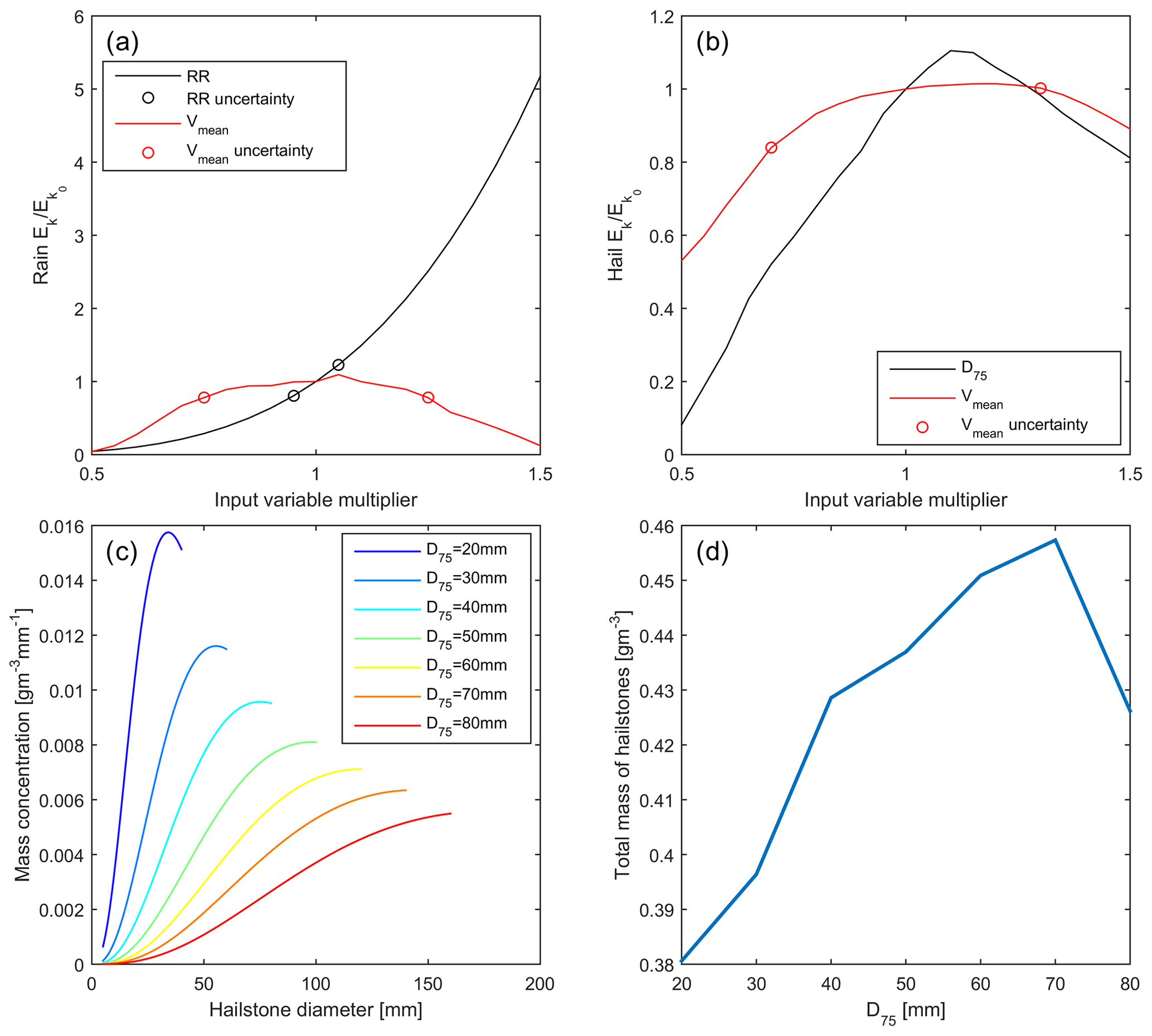
Figure 8 Sensitivities of rain (a) and hail (b) impact kinetic energies in one 5 min period to the application of ±50 % uncertainties on the input parameters; wind speed (V_mean) and precipitation intensity (RR) or hail diameter (D₇₅). Circles represent reported uncertainties in radar retrievals of wind speed (Fast et al., 2008) and rainfall rate (see Table 1 in Seo and Krajewski, 2010). (c) Mass concentrations of hailstones per cubic meter of air (expressed as dM∕dD) associated with a range of D₇₅ values as a function of hailstone diameter. (d) Total hail mass (in grams) per cubic meter of air as a function of D₇₅.

4 Conclusions

A robust and flexible framework has been developed and presented for generating an observationally constrained georeferenced assessment of precipitation-induced wind turbine blade leading edge erosion potential. The approach elaborated herein is naturally subject to a range of uncertainties but is automated, objective, repeatable and predicated on publicly available data available from across most of the continental US. Further, the modular structure means it is flexible to use with different assumptions and/or data streams. Although the data volumes are not trivial (see Appendix A), this analysis framework could be applied to NWS radar data to estimate LEE potential at any arbitrary site in CONUS and/or applied to data from other national dual-polarization radar networks for other regions of the world. For example, the Network of European Meteorological Services (EUMETNET) operates over 200 radars many of which have been upgraded to dual polarization (Saltikoff et al., 2018). The tool proposed here could be used to provide a first assessment of the erosion climate in which a given sited turbine may operate. It thus provides an important first step towards enabling an assessment of the threat of excessive precipitation-induced LEE in a given deployment environment and the cost effectiveness of options to reduce the likelihood of premature blade damage.

The actual likelihood of excess WT LEE and blade damage in any environment is not only a function of the precipitation and wind climate but also of the WT dimensions, materials used in the blade coatings and the coating thickness (Eisenberg et al., 2018; Slot et al., 2015), the presence of existing microstructural defects (Evans et al., 1980) due to manufacturing defects and damage during transportation (Keegan et al., 2013; Nelson et al., 2017), and other aspects of the operating environment (including thermal fatigue and the occurrence of icing; Slot et al., 2015).

The preliminary estimates of erosion potential and the partitioning between liquid precipitation and hail are naturally subject to limitations including, in likely order of importance, the following:

• the relatively short duration of time for which the dual-polarization radar products are available. The upgrade of the NWS radar network to dual polarization was completed in April 2013; thus only the complete years of 2014–2018 (inclusive) were available for analysis. Given the large interannual variability in precipitation climates, this is too short to build a comprehensive climatology (Karl et al., 1995; Prein and Holland, 2018). Any geospatial depiction of the potential precipitation erosion climate will vary according to the precise data period used to compute the climatology and may evolve as a result of climate non-stationarity altering aspects of the precipitation climate (e.g., the probability of hail, Brimelow et al., 2017, and rainfall intensity, Easterling et al., 2000).

• the applicability of the radar-derived wind speed estimates to derive wind turbine blade rotational speed. There are considerable challenges to line-of-sight wind retrievals from radar (Fast et al., 2008). The approach adopted herein assumes a uniform wind flow pattern to derive the wind speeds at the nominal wind turbine hub height, which may not be realized. As described above, while the wind speed climates at five of the six locations considered exhibited relatively good agreement with previous estimates of wind climates, values for the location in Texas are negatively biased. This likely results in a negative bias in kinetic energy transfer for this site.

• assumptions regarding the size distribution, occurrence and terminal velocities of hail (Dessens et al., 2015; Allen et al., 2017; Heymsfield et al., 2014). The evolution of the NWS radar network to dual polarization provides an unprecedented opportunity for spatial estimates of hail presence and size in clouds (Kumjian et al., 2018). However, hail production is a complex and incompletely understood phenomenon (Dennis and Kumjian, 2017; Blair et al., 2017; Pruppacher and Klett, 2010). There are substantial event-to-event variations in the size distribution and density of hail stones (Heymsfield et al., 2014), in the presence of solid-phase hydrometeors in clouds (as detected by radar) and the occurrence of hail at the ground (Kumjian et al., 2019). Estimates of hail occurrence, size distribution and terminal fall velocity presented herein are likely conservative (i.e., upper bounds on true values), and thus LEE may be overestimated.

• assumptions regarding the size distribution of rain droplets. Most observational studies indicate an exponential form (Uijlenhoet, 2001), and the Marshall–Palmer distribution is the most widely applied. However, a range of different forms have been proposed to describe the size spectrum of rain droplets (dN∕dR) including gamma (Ulbrich, 1983) and lognormal (Feingold and Levin, 1986), an alternative exponential form (Best, 1950), and more complex non-parametric forms (Morrison et al., 2019). There is also evidence that droplet size distributions may exhibit a functional dependence on near-surface wind speed (Testik and Pei, 2017).

• assumptions applied in deriving precipitation intensity and other precipitation properties from radar. Notable event-to-event variations in the applicability of Z–R relationships have been reported during rain (Uijlenhoet, 2001; Villarini and Krajewski, 2010).

Future work could address and reduce these uncertainties and adapt this approach to examine different wind turbines (by applying a different RPM curve) and/or to assimilate different atmospheric data and/or incorporate more explicit aspects of material response. In this analysis we have chosen to focus on an energetic approach in which we compute the accumulated kinetic energy transmitted to the blade leading edge instead of using approaches based on the waterhammer equation that seek to compute the impact pressure and material response to the resulting Rayleigh, shear and compression waves (that are assumed to act independently of each individual impact) (Slot et al., 2015; Dashtkar et al., 2019). It is important to reiterate that the approach adopted here, i.e., to compute the maximum total kinetic energy transferred to the blade, which is used here as a proxy for the erosion potential, represents the upper bound on actual kinetic energy transfer since it employs a closing velocity characteristic for the tip of WT rotors, assumes all falling hydrometeors impact the blade, and neglects energy loss during the transfer, “splash” and bounce of hydrometeors. There are more complex frameworks that can be applied to simulate the pressure and transient stresses on the blade coatings (Mishnaevsky Jr., 2019) and impingement erosion (Amirzadeh et al., 2017a, b). A model of the blade response to precipitation impacts could be incorporated within the analysis framework to examine the probability and time to exceed the (cumulative) failure threshold energy (Fiore et al., 2015).

This work suggests the dominance of hail as a damage vector for WT blades at all of the sites studied here. This is consistent with indications that deep convection and hail are particularly common in the central US (Cintineo et al., 2012) and indications of large geographic variability in hail frequency (Ni et al., 2017). This finding emphasizes the key importance of efforts to build and enhance hail climatologies (Allen et al., 2015; Gagne et al., 2019) with applications in a wide range of industries (from insurance to renewable energy). The dominance of hail as a damage vector and the importance of a relatively small number of 5 min periods to total annual kinetic energy transfer from rain adds credence to the proposal that blade LEE could be greatly reduced by operating erosion-safe turbine control (Bech et al., 2018), wherein the WTs are curtailed during periods with extreme precipitation (very heavy rain or the occurrence of hail) without substantial loss of income.

Appendix A

The workflow, NWS radar data products and data volumes necessary for the components of the precipitation erosion climate are as follows:

• 1.

  Download daily .tar archives of NEXRAD polarized Doppler radar data using ftp from the data repository hosted at https://www.ncdc.noaa.gov/nexradinv/ (last access: 7 January 2019; NOAA, 1991). These tar archives contain all NEXRAD level 2 and 3 data and data products at 5 min intervals in binary NEXRAD format. The 365 daily tar comprise 60–100 GB per station per year (PSPY).

• 2.

  Preprocessing:

  • a.

    Extract precipitation rates (N1P) and hail reports (NHI) files from each daily tar file.

  • b.

    Import raw files into NOAA Weather and Climate Toolkit (https://www.ncdc.noaa.gov/wct/, 15 January 2020; NOAA NCEI, 2020a), translate N1P, N0V and NHI files into netcdf and .csv, file sizes and numbers:

    • -

      hydrometeor classification (HHC) raw files (32 000 to 70 000 files PSPY, 124–180 MB PSPY)

    • -

      NHI csv files (12 000 to 137 000 files PSPY, totaling 25–190 MB PSPY)

    • -

      N1P raw files (68 000 to 90 000 files PSPY, totaling 600–900 MB PSPY)

    • -

      N1P netcdf files (130 000 to 150 000 files PSPY, totaling 240–290 GB PSPY)

    • -

      base wind speed (N0V) raw files (40 000 to 60 000 files PSPY, totaling 35–45 GB PSPY)

    • -

      N0V netcdf files (40 000 to 60 000 files PSPY, totaling 900–1100 MB PSPY).

Subsequent data analysis is conducted within MATLAB.