Actuator line simulations of wind turbine wakes using the lattice Boltzmann method

The high computational demand of large-eddy simulations (LESs) remains the biggest obstacle for a wider applicability of the method in the field of wind energy. Recent progress of GPU-based (graphics processing unit) lattice Boltzmann frameworks provides significant performance gains alleviating such constraints. The presented work investigates the potential of LES of wind turbine wakes using the cumulant lattice Boltzmann method (CLBM). The wind turbine is represented by the actuator line model (ALM). The implementation is validated and discussed by means of a code-to-code comparison to an established finite-volume Navier–Stokes solver. To this end, the ALM is subjected to both laminar and turbulent inflow while a standard Smagorinsky sub-grid-scale model is employed in the two numerical approaches. The resulting wake characteristics are discussed in terms of the first- and second-order statistics as well the spectra of the turbulence kinetic energy. The near-wake characteristics in laminar inflow are shown to match closely with differences of less than 3 % in the wake deficit. Larger discrepancies are found in the far wake and relate to differences in the point of the laminar-turbulent transition of the wake. In line with other studies, these differences can be attributed to the different orders of accuracy of the two methods. Consistently better agreement is found in turbulent inflow due to the lower impact of the numerical scheme on the wake transition. In summary, the study outlines the feasibility of wind turbine simulations using the CLBM and further validates the presented set-up. Furthermore, it highlights the computational potential of GPU-based LBM implementations for wind energy applications. For the presented cases, near-real-time performance was achieved using a single, off-the-shelf GPU on a local workstation.

1 Introduction

Large-eddy simulations (LESs) can provide valuable insights into the aerodynamic interaction of wind turbines. In comparison to modelling approaches with lower fidelity, LESs allow for the investigation of aerodynamic effects that are directly associated with the transient nature of highly turbulent flows as found in the atmospheric boundary layer (ABL). Resolving the transient large energy-containing turbulent structures does, however, come at a high computational cost that is far beyond, for instance, that of Reynolds-averaged approaches (RANS; Mehta et al., 2014). Still, in recent years, LESs have been increasingly used in engineering-driven contexts, such as, for instance, the investigation of fatigue loads in various operating conditions (Storey et al., 2016; Nebenführ and Davidson, 2017; Meng et al., 2018), the effects of turbine curtailment (Nilsson et al., 2015; Fleming et al., 2015; Dilip and Porté-Agel, 2017), or the development and testing of farm-wide optimization control strategies (Ciri et al., 2017; Munters and Meyers, 2018). With such applications the computational demand of typical case studies increases dramatically when compared to the more fundamental investigations performed in earlier years of LES of the ABL. This increase in computational demand relates both to the size of considered domains and to the physical time simulated. Examples of the former are simulations of entire offshore wind farms (Churchfield et al., 2012b; Abkar and Porté-Agel, 2013; Nilsson et al., 2015) or large areas of complex orography (Ivanell et al., 2018; Fang et al., 2018). An extreme example of the latter is the work by Abkar et al. (2016) investigating the wakes in a wind farm throughout two diurnal cycles.

Despite the growing capacities of modern high-performance-computing (HPC) clusters, computational power remains the biggest bottleneck for such large-scale LES applications. Over the last 3 decades the lattice Boltzmann method (LBM) has evolved into a viable alternative to classical computational fluid dynamics (CFD) approaches with significantly increased computational performance (Malaspinas and Sagaut, 2014; Krüger et al., 2016). This largely relates to the strict separation of non-linear and non-local terms, allowing for excellent parallelizability (Succi, 2015). The LBM, therefore, also proves to be perfectly suitable for implementations on graphics processing units (GPU). Various authors documented the substantial speed-up factors of such implementations; see, e.g. Schönherr et al. (2011), Obrecht et al. (2013), or Onodera and Idomura (2018), to name a few. Nevertheless, applications of the LBM in the field of ABL flows and wind energy are still rare compared to other fields of fluid dynamics. To date, one of the few prominent applications in the wider field of atmospheric flows are wind comfort assessments and pollution dispersion in urban canopies (e.g. King et al., 2017; Ahmad et al., 2017; Jacob and Sagaut, 2018; Lenz et al., 2019; Merlier et al., 2018, 2019). Other related applications are wind load assessments as presented by Andre et al. (2015), Fragner and Deiterding (2016), or Mohebbi and Rezvani (2018). In the field of wind energy though, the use of the LBM remains rather limited. Deiterding and Wood (2016), Khan (2018), and Zhiqiang et al. (2018) presented simulations of geometrically resolved model-scale wind turbines. Avallone et al. (2018) and van der Velden et al. (2016) on the other hand investigated noise emissions of blade sections. Various fundamental aspects of the LBM in the context of wind energy and particularly wind farm simulations therefore remain untouched yet crucial for future applications.

One method of special importance for the modelling of wind turbines in LES is the actuator line model (ALM). The ALM, as well as other actuator-type models, couple a CFD simulation to an extension of the blade element momentum (BEM) method. Using the locally sampled flow velocity, body forces of a blade element are computed using empirically determined lift and drag coefficients of the referring aerofoil section. These are then again applied in the domain of the CFD simulation (Sørensen and Shen, 2002; Troldborg et al., 2010). This avoids prohibitively expensive geometrically resolved simulations of the rotor. It is therefore the only feasible way to represent wind turbines in LES on a wind farm scale today (Sanderse et al., 2011; Mehta et al., 2014). Again, fundamental investigations of the ALM in lattice Boltzmann frameworks are still limited, yet crucial for future simulations of entire wind farms. Rullaud et al. (2018) presented a first conceptual study of the ALM in this context. The presented ALM for vertical-axis wind turbines was, however, limited to two dimensions, i.e. cross-sectional planes. More recently, Asmuth et al. (2019) presented an initial fundamental investigation of the classical ALM for horizontal-axis turbines in a cumulant lattice Boltzmann framework in uniform laminar inflow. The main aspects of the study were the sensitivity of the blade forces of the ALM to the spatial and temporal resolution of the bulk scheme as well as computational performance.

The objective of this paper is to analyse the wake of a single wind turbine simulated with the ALM and the cumulant lattice Boltzmann method (CLBM), a recently developed high-fidelity collision operator that is particularly suited for high-Reynolds-number flows (Geier et al., 2015, 2017b). The main portion of the presented study is based on a code-to-code comparison to a standard finite-volume (FV) Navier–Stokes (NS) solver. The primary motivation for this is to extend the aforementioned validation study of this ALM implementation (Asmuth et al., 2019) to the near- and far-wake characteristics. The comparison comprises laminar and turbulent inflow cases, respectively. Furthermore, using the same set-up, we briefly evaluate the impact of a stabilizing limiter within the collision operator on the wake characteristics.

To the authors' knowledge, this study constitutes the first application of the CLBM to wind turbine wake simulations. Moreover, application-oriented studies of the utilized parameterized version of this collision operator (as further outlined in Sect. 2) are generally still limited; see Lenz et al. (2019). Therefore, a further motivation of the study is to show the general potential of wind turbine wake simulations using the LBM and specifically the CLBM. The numerical stability of such simulations using the LBM is not self-evident when using typical, rather coarse grid resolutions.

The remainder of the paper is organized as follows: Sect. 2 provides a brief introduction to the LBM. This includes a description of the underlying numerical concept, characteristics of the cumulant collision model, the use of turbulence models in the CLBM, and, lastly, details on the implementation of the ALM. Section 3 describes the utilized numerical frameworks and case set-up. In Sect. 4 we present the code-to-code comparison in laminar inflow. A discussion of the results in turbulent inflow is given in Sect. 5. The impact of the third-order cumulant limiter is outlined in Sect. 6. Section 7 briefly touches upon aspects of computational performance. Lastly, final conclusions and guidelines for future studies are provided in Sect. 8.

2 The lattice Boltzmann method

In the following we provide a brief description of the LBM. This comprises a description of the governing equations as well as more specific topics relevant for the presented studies, such as sub-grid-scale (SGS) modelling and the implementation of the ALM. For a more detailed description of the fundamentals, the interested reader is referred to the work by Krüger et al. (2016).

2.1 Governing equations

The LBM solves the kinetic Boltzmann equation, i.e. the transport equation of particle distribution functions (PDFs) f in physical and velocity space. PDFs describe the probability of encountering a particle (mass) density of velocity ξ at time t at location x. Solving the kinetic Boltzmann equation thus requires a discretization in both physical and velocity space. Using a finite set of discrete velocities (referred to as velocity lattice; see Fig. 1) and discretizing in space and time, one obtains the lattice Boltzmann equation (LBE) in index notation

$$\begin{array}{}\text{(1)}& f_{ijk}\left(t+\mathrm{\Delta }t,\mathit{x}+\mathrm{\Delta }t{\mathit{e}}_{ijk}\right)-f_{ijk}(t,\mathit{x})={\mathrm{\Omega }}_{ijk}(t,\mathit{x}),\end{array}$$

where

$$\begin{array}{}\text{(2)}& {\mathit{e}}_{ijk}=(ic,jc,kc)\end{array}$$

is the particle velocity vector and i, j, $k\in \mathit{\{}-\mathrm{1}$, 0, 1}. The lattice speed c is chosen such that

$$\begin{array}{}\text{(3)}& c=\mathrm{\Delta }x/\mathrm{\Delta }t.\end{array}$$

On uniform Cartesian grids PDFs are therefore inherently advected from their source (black dot in Fig. 1) to the neighbouring nodes during one time step avoiding any interpolation in the advection. The collision operator Ω_ijk on the right-hand side models the redistribution of f through particle collisions within the control volume. Based on kinetic theory the collision process is modelled as a relaxation of particle distribution functions towards an equilibrium. In the classical and most simple collision model, the single-relaxation-time (SRT) model, commonly referred to as the lattice Bhatnagar–Gross–Kroog (LBGK) model (Bhatnagar et al., 1954), all PDFs are relaxed towards an equilibrium using a single constant relaxation time τ, viz.

$$\begin{array}{}\text{(4)}& {\mathrm{\Omega }}_{ijk}(t,\mathit{x})=-{\displaystyle \frac{\mathrm{\Delta }t}{\mathit{\tau }}}\left(f_{ijk}(t,\mathit{x})-f_{ijk}^{\mathrm{eq}}(t,\mathit{x})\right).\end{array}$$

The equilibrium distribution $f_{ijk}^{\mathrm{eq}}$ is given by the second-order Taylor expansion of the Maxwellian equilibrium

$$\begin{array}{}\text{(5)}& f_{ijk}^{\mathrm{eq}}=w_{ijk}\mathit{\rho }\left(\mathrm{1}+{\displaystyle \frac{\mathit{u}\cdot {\mathit{e}}_{ijk}}{c_{\mathrm{s}}^{\mathrm{2}}}}+{\displaystyle \frac{{\left(\mathit{u}\cdot {\mathit{e}}_{ijk}\right)}^{\mathrm{2}}}{\mathrm{2}{c}_{\mathrm{s}}^{\mathrm{4}}}}-{\displaystyle \frac{\mathit{u}\cdot \mathit{u}}{\mathrm{2}{c}_{\mathrm{s}}^{\mathrm{2}}}}\right),\end{array}$$

where c_s is the lattice speed of sound and u and ρ the macroscopic velocity and density, respectively. The weights w_ijk are specific to the velocity lattice and ensure mass and momentum conservation of the equilibrium.

Figure 1 Schematic of three-dimensional velocity lattices. Coordinate-normal planes marked in yellow. Each vector refers to a discrete velocity e_ijk as given in Eq. (1). Velocities of the D3Q19 lattice (Qian et al., 1992) with 19 discrete directions are given by orange vectors. Additional velocity directions considered in the D3Q27 lattice are given by red vectors.

Macroscopic quantities can generally be obtained from the raw velocity moments of the PDFs:

$$\begin{array}{}\text{(6)}& m_{\mathit{\alpha }\mathit{\beta }\mathit{\gamma }}=\sum _{i=-\mathrm{1}}^{\mathrm{1}}\sum _{j=-\mathrm{1}}^{\mathrm{1}}\sum _{k=-\mathrm{1}}^{\mathrm{1}}\left(ic{)}^{\mathit{\alpha }}\right(jc{)}^{\mathit{\beta }}(kc{)}^{\mathit{\gamma }}{f}_{ijk},\end{array}$$

with α, β, and γ denoting the order of the moment in the referring lattice direction and $\mathit{\alpha }+\mathit{\beta }+\mathit{\gamma }$ the total order of the moment. Following from dimensional analysis the macroscopic mass density ρ is given by the zeroth-order moment m₀₀₀. Analogously, the momentum in x, y, and z is obtained from the first-order moment in the reference coordinate directions m₁₀₀, m₀₁₀, and m₀₀₁, respectively. The macroscopic velocity and density required for the computation of $f_{ijk}^{\mathrm{eq}}$ can thus be obtained locally from the PDFs. Furthermore, starting from a moment expansion of the LBE itself we can show via a Chapman–Enskog expansion that it recovers the (weakly compressible) Navier–Stokes equations on the macroscopic level. For the sake of brevity details upon the latter are omitted here. A comprehensive overview can be found in Krüger et al. (2016). Nevertheless, it should be noted that

$$\begin{array}{}\text{(7)}& \mathit{\tau }={\displaystyle \frac{\mathrm{1}}{\mathit{\omega }}}=\mathrm{3}\mathit{\nu }/c^{\mathrm{2}}+\mathrm{\Delta }t/\mathrm{2},\end{array}$$

with ν being the kinematic viscosity and ω the relaxation rate (He and Luo, 1997; Dellar, 2001).

In summary, the simplicity of the LBM leads to a straightforward explicit algorithm. Numerically, it is realized by decomposing and rearranging Eqs. (1) and (4) into two separate parts. The first becomes the collision step

$$\begin{array}{}\text{(8)}& f_{ijk}^{*}(t,\mathit{x})=\left(\mathrm{1}-{\displaystyle \frac{\mathrm{\Delta }t}{\mathit{\tau }}}\right)f_{ijk}(t,\mathit{x})+{\displaystyle \frac{\mathrm{\Delta }t}{\mathit{\tau }}}{f}_{ijk}^{\mathrm{eq}}(t,\mathit{x}),\end{array}$$

where $f_{ijk}^{*}$ is the post-collision distribution function. And the second is the streaming (or propagation) step

$$\begin{array}{}\text{(9)}& f_{ijk}\left(t+\mathrm{\Delta }t,\mathit{x}+\mathrm{\Delta }t{\mathit{e}}_{ijk}\right)=f_{ijk}^{*}(t,\mathit{x})\end{array}$$

advecting $f_{ijk}^{*}$ to the neighbouring nodes.

2.2 The cumulant collision model

Due to poor numerical stability of the original LBGK model, various alternative approaches have been presented. These mostly relate to the class of multiple-relaxation-time (MRT) models; see for instance Lallemand and Luo (2000) and d'Humières et al. (2002). MRT models transform the pre-collision PDFs f_ijk (Eq. 8) into a velocity moment space. Each moment is then relaxed individually towards a referring equilibrium moment $m_{\mathit{\alpha }\mathit{\beta }\mathit{\gamma }}^{\mathrm{eq}}$. The individual relaxation rates of the hydrodynamic moments (up to second order) remain physically motivated with the second-order relaxation rate given by Eq. (4). Relaxation rates of higher-order moments, though, can be tuned freely. Subsequently, the moments are transformed back into particle distribution space and advected following Eq. (9).

Despite significant stability improvements, several fundamental deficiencies of MRT models render the approach unsuitable for high-Reynolds-number flows as required for studies of wind turbines in the ABL. Referring to the seminal paper by Geier et al. (2015) such deficiencies include, among others, the lack of a universal formulation for optimal collision rates, deficiencies stemming from the rather arbitrary choice of moment space, lack of Galilean invariance, and introduction of hyper-viscosities. Deteriorations of the flow field through local instabilities can be the consequence (Gehrke et al., 2017). To remedy the aforementioned deficiencies, Geier et al. (2015) suggest a universal formulation based on statistically independent observable quantities (cumulants) of the PDFs, i.e. the CLBM. After performing the two-sided Laplace transform of the pre-collision PDFs

$$\begin{array}{}\text{(10)}& F\left(\mathbf{\Xi }\right)=\mathcal{L}\left(f\right(\mathit{\xi }\left)\right)=\underset{-\mathrm{\infty }}{\overset{\mathrm{\infty }}{\int }}f\left(\mathit{\xi }\right)e^{-\mathbf{\Xi }\cdot \mathit{\xi }}d\mathit{\xi },\end{array}$$

with Ξ={Ξ, Υ, Z} denoting the particle velocity ξ={ξ, υ, ζ} in wave number space, cumulants c_αβγ can be obtained as

$$\begin{array}{}\text{(11)}& c_{\mathit{\alpha }\mathit{\beta }\mathit{\gamma }}=c^{-\mathit{\alpha }-\mathit{\beta }-\mathit{\gamma }}{\displaystyle \frac{{\partial }^{\mathit{\alpha }}{\partial }^{\mathit{\beta }}{\partial }^{\mathit{\gamma }}}{\partial {\mathrm{\Xi }}^{\mathit{\alpha }}\partial {\mathrm{{\rm Y}}}^{\mathit{\beta }}\partial Z^{\mathit{\gamma }}}}\ln \left(F\right(\mathrm{\Xi },\mathrm{{\rm Y}},Z\left)\right).\end{array}$$

Subsequently, cumulants are relaxed towards the reference equilibrium:

$$\begin{array}{}\text{(12)}& c_{\mathit{\alpha }\mathit{\beta }\mathit{\gamma }}^{*}={\mathit{\omega }}_{\mathit{\alpha }\mathit{\beta }\mathit{\gamma }}{c}_{\mathit{\alpha }\mathit{\beta }\mathit{\gamma }}^{\mathrm{eq}}+\left(\mathrm{1}-{\mathit{\omega }}_{\mathit{\alpha }\mathit{\beta }\mathit{\gamma }}\right)c_{\mathit{\alpha }\mathit{\beta }\mathit{\gamma }}.\end{array}$$

Here, $c_{\mathit{\alpha }\mathit{\beta }\mathit{\gamma }}^{*}$ denotes the post-collision cumulant and ω_αβγ the reference relaxation rate. As shown by Geier et al. (2015), the statistical independence of cumulants unconditionally eliminates the MRT's deficiencies such as the dependency of Galilean invariance and occurrence of hyper-viscosities on the choice of relaxation rates.

A simple and widely adopted choice in the CLBM is to set all relaxation rates of higher-order cumulants to 1, commonly referred to as the AllOne cumulant. In this case, higher-order cumulants are instantly relaxed towards the reference equilibrium. This unconditionally damps all higher-order perturbations, providing an inherently stable solution and thereby an extremely robust numerical framework. Numerous studies have shown that the AllOne CLBM can be readily applied to high-Reynolds-number flows (see Geier et al., 2015; Far et al., 2016; Gehrke et al., 2017; Kutscher et al., 2019; Onodera and Idomura, 2018). A further development of the original AllOne is the parameterized CLBM presented in Geier et al. (2017b). Based on the theory of the so-called magic parameter (Ginzburg and Adler, 1994; Ginzburg et al., 2008), the authors derived a parametrization to optimize the higher-order relaxation rates. The same authors show that the parametrization increases the convergence of the CLBM in diffusion to the fourth order under diffusive scaling (i.e. Δt∝Δx²). However, unconditional numerical stability is no longer guaranteed and requires the use of a limiter as outlined in Sect. 2.4.

From a theoretical point of view the parameterized CLBM can arguably be seen as one of the most advanced collision models today, in terms of both accuracy and stability. Nevertheless, the complexity of the collision model makes it more computationally demanding in terms compared to SRT and MRT models. Furthermore, the CLBM is only defined on the D3Q27 velocity lattice as opposed to SRT and MRT models that typically employ D3Q19 lattices. Consequently, it also requires more memory. In addition to the aforementioned theoretical considerations, we therefore provide a pre-study on the suitability of other collision models for this application in Sect. A.

2.3 Nondimensionalization

For the sake of simplicity as well as numerical efficiency and accuracy, implementations of the LBM are commonly nondimensionalized. Physical units are therefore rescaled to non-dimensional lattice units (hereafter indexed (⋅)^LB) with $c^{\mathrm{LB}}=\mathrm{\Delta }{x}^{\mathrm{LB}}/\mathrm{\Delta }{t}^{\mathrm{LB}}=\mathrm{1}$. Hence, we can derive scaling factors C for all relevant physical units. As the LBM generally states a weakly compressible method, these are the Reynolds and Mach numbers Re and Ma, respectively. Within this study we use the cell Reynolds number as $R{e}_{\mathrm{c}}=u_{\mathrm{0}}\mathrm{\Delta }x/\mathit{\nu }$, where u₀ is the inflow velocity at the inlet and Δx grid spacing. The Mach number is consequently given by u₀ and the lattice speed of sound c_s: $Ma=u_{\mathrm{0}}/c_{\mathrm{s}}$. Starting from the spatial scaling factor we obtain $C_x=\mathrm{\Delta }x/\mathrm{\Delta }{x}^{\mathrm{LB}}=L_i/n_i$, where L_i is the length of the domain and n_i the number of grid points in the reference spatial dimension. With $c_{\mathrm{s}}^{\mathrm{LB}}=c/\sqrt{\mathrm{3}}$, the reference velocity on the lattice is given by $u_{\mathrm{0}}^{\mathrm{LB}}=Ma/\sqrt{\mathrm{3}}$, yielding the velocity scaling factor $C_{\mathrm{u}}=\sqrt{\mathrm{3}}{u}_{\mathrm{0}}/Ma$. It follows that the temporal scaling factor is given by $C_{\mathrm{t}}=C_x/C_{\mathrm{u}}$, which implies a physical time step Δt=C_tΔt^LB that is inherently proportional to the grid spacing and Mach number. The viscosity in lattice units becomes ${\mathit{\nu }}^{\mathrm{LB}}=\mathit{\nu }{C}_{\mathrm{t}}/C_x^{\mathrm{2}}$. The order of magnitude of ν^LB thus directly depends on the choice of grid resolution and Mach number.

In this study we employ the LBM for an incompressible problem. As in the majority of applications, this implies that compressibility effects are assumed to have negligible effects on the flow physics of interests. The Mach number is thus merely required to be small, yet does not necessarily have to comply with the physically correct value of the problem. For incompressible flows it therefore commonly reduces to a somewhat free parameter affecting numerical accuracy in the incompressible limit (Dellar, 2003; Geier et al., 2015, 2017b), computational demand by means of the time step, and the magnitude of the viscosity on the lattice level.

2.4 Sub-grid-scale modelling in the LBM

Early on, LES approaches were used in LBM frameworks (see, e.g. Hou et al., 1996). The most common choice are eddy-viscosity approaches that are simply adopted from NS frameworks and incorporated by adding the eddy viscosity ν_t to the shear viscosity ν in Eq. (7). Examples thereof range from the standard Smagorinsky model (Hou et al., 1996; Krafczyk et al., 2003) to more advanced models like the wall-adapting local eddy-viscosity model (WALE; Weickert et al., 2010), the shear-improved Smagorinsky model (SISM; Jafari and Mohammad, 2011), and dynamic Smagorinsky approaches (Premnath et al., 2009b). Others, on the other hand, suggested LB-specific methods based on the approximate deconvolution of the LBE itself (Sagaut, 2010; Malaspinas and Sagaut, 2011; Nathen et al., 2018).

2.4.1 Implementation of eddy-viscosity models

Using a standard constant Smagorinsky model, the eddy viscosity can be determined locally using the well-known formulation

$$\begin{array}{}\text{(13)}& {\mathit{\nu }}_{\mathrm{t}}={\left(C_{\mathrm{s}}\mathrm{\Delta }\right)}^{\mathrm{2}}\stackrel{\mathrm{‾}}{S},\end{array}$$

where C_s is the Smagorinsky constant, Δ the filter width (here referring to the grid spacing Δx), and $\stackrel{\mathrm{‾}}{S}$ the second invariant of the filtered strain rate tensor

$$\begin{array}{}\text{(14)}& {\stackrel{\mathrm{‾}}{S}}_{ij}={\displaystyle \frac{\mathrm{1}}{\mathrm{2}}}\left({\displaystyle \frac{\partial \stackrel{\mathrm{‾}}{u_i}}{\partial x_j}}+{\displaystyle \frac{\partial \stackrel{\mathrm{‾}}{u_j}}{\partial x_i}}\right),\mathrm{with}\stackrel{\mathrm{‾}}{S}=\sqrt{\mathrm{2}{\stackrel{\mathrm{‾}}{S}}_{ij}{\stackrel{\mathrm{‾}}{S}}_{ij}}.\end{array}$$

A clear advantage of the LBM over NS approaches in this context is the local availability of the strain rate tensor. Using the second-order moments or cumulants of the local PDFs, the components of ${\stackrel{\mathrm{‾}}{S}}_{ij}$ can be determined without finite differencing. Further details on the determination of ${\stackrel{\mathrm{‾}}{S}}_{ij}$ in cumulant space can be found in Geier et al. (2015, 2017b). It should be noted, though, that the strain rates in the CLBM and most MRT models are dependent on the total shear viscosity (${\mathit{\nu }}_{\mathrm{tot}}=\mathit{\nu }+{\mathit{\nu }}_{\mathrm{t}}$) and the bulk viscosity. As opposed to the SRT, where ${\stackrel{\mathrm{‾}}{S}}_{ij}$ is only dependent on the total shear viscosity, it is therefore not possible to explicitly determine ν_t. Hence, the eddy viscosity ν_t(t) can be computed either explicitly, using ν_t(t−Δt), or iteratively. Yu et al. (2005), however, showed that the error associated with the implicitness of ν_t is generally negligible due to the typically small time steps used in the LBM. We shall therefore refrain from implicitly solving for ν_t, in line with similar Smagorinsky approaches in MRT frameworks (Yu et al., 2006; Premnath et al., 2009a).

2.4.2 Stabilizing limiter in the cumulant LBM

A crucial characteristic of the CLBM is the model's inherent numerical stability. As opposed to many other collision models, it does not require the stabilizing features of explicit turbulence models, even for under-resolved highly turbulent flows. The stabilizing characteristic of the original AllOne cumulant approach appears rather obvious as it unconditionally resets all higher-order cumulants in each time step. The fourth-order accuracy of the parameterized approach, however, relies on the temporal memory of these higher-order cumulants. Therefore, Geier et al. (2017b) suggest the use of a limiter λ_m that is only applied to the relaxation of the third-order cumulants. The relaxation rates of these cumulants, subsequently referred to as ω_m, are consequently substituted by

$$\begin{array}{}\text{(15)}& {\mathit{\omega }}_{\mathit{\zeta }}={\mathit{\omega }}_{\mathrm{m}}+{\displaystyle \frac{\left(\mathrm{1}-{\mathit{\omega }}_{\mathrm{m}}\right)\left|c_{\mathrm{m}}\right|}{\mathit{\rho }{\mathit{\lambda }}_{\mathrm{m}}+\left|c_{\mathrm{m}}\right|}},\end{array}$$

where $\left|c_{\mathrm{m}}\right|$ refers to the magnitude of the respective third-order cumulant. Destabilizing accumulation of energy in these cumulants is hereby inhibited as ω_ζ approaches 1 for $\mathit{\rho }{\mathit{\lambda }}_{\mathrm{m}}\ll \left|c_{\mathrm{m}}\right|$. Nonetheless, the order of the error introduced by the limiter lies well below the leading error of the LBM itself. The fourth-order accuracy of the scheme is thus not affected in the asymptotic limit. Like the AllOne version, the parameterized CLBM therefore does not require the numerically stabilizing features of an explicit sub-grid-scale model, yet with a higher order of accuracy. In this study we shall therefore focus on the investigation of the parameterized CLBM.

2.5 Implementation of the actuator line model in lattice Boltzmann frameworks

The lattice Boltzmann actuator line implementation used in this study closely follows the original description in NS frameworks as presented by Sørensen and Shen (2002). The forces acting on the rotor are determined using the local relative velocity u_rel of the respective blade elements along the actuator line. The relative velocity is computed from the sampled velocity in the blade-normal (stream-wise) and tangential directions u_n and u_θ, respectively, using

$$\begin{array}{}\text{(16)}& u_{\mathrm{rel}}=\sqrt{u_{\mathrm{n}}^{\mathrm{2}}+{\left(\mathrm{\Omega }r-u_{\mathit{\theta }}\right)}^{\mathrm{2}}},\end{array}$$

where Ω is the rotational velocity of the turbine and r the radial position of the blade element. The local blade force per unit length then reads

$$\begin{array}{}\text{(17)}& \mathit{F}=\mathrm{0.5}\mathit{\rho }{u}_{\mathrm{rel}}^{\mathrm{2}}{c}_{\mathrm{a}}\left(C_{\mathrm{L}}{\mathit{e}}_{\mathrm{L}}+C_{\mathrm{D}}{\mathit{e}}_{\mathrm{D}}\right),\end{array}$$

with e_L,D being the unit vector in the direction of the lift and drag force and c_a being the chord length of the reference aerofoil section. The lift and drag coefficients C_L and C_D are provided from tabulated aerofoil data as functions of the local angle of attack and Reynolds number. The resulting blade forces are subsequently applied across a volume in the flow field by taking the convolution integral of F with a Gaussian regularization kernel η_ϵ, given by

$$\begin{array}{}\text{(18)}& {\mathit{\eta }}_{\mathit{ϵ}}={\displaystyle \frac{\mathrm{1}}{{\mathit{\pi }}^{\mathrm{3}/\mathrm{2}}{\mathit{ϵ}}^{\mathrm{2}}}}{e}^{-(d/\mathit{ϵ}{)}^{\mathrm{2}}},\end{array}$$

where ϵ adjusts the width of the regularization and d is the distance from the centre of the blade element to the point in space where the force is applied. The resulting force is applied at each grid node by simply adding the respective component of Δt∕2F to the pre-collision first-order cumulants. For the sake of completeness it should be noted that body force formulations generally depend on the collision model. See, for instance, Buick and Greated (2000) and Guo et al. (2008) for a description in SRT and MRT frameworks, respectively.

Differences between ALM implementations in NS and LBM frameworks are obviously small. The latter can be expected given that the link between the model itself and the flow solver is simply made by exchanging information of velocity and body forces. Lastly, it is worth mentioning that the locality of all subroutines of the ALM allows for a perfect parallelization. The model is therefore efficiently parallelized on the GPU, in line with the general architecture of the utilized LBM solver (see Sect. 3.1) using Nvidia's CUDA toolkit.

3 Numerical set-up

In light of the code-to-code comparison, the simulations in both frameworks were set up in the most similar manner possible. This refers to the grid, the boundary conditions, and the implementation of the ALM. Nevertheless, certain differences remain unavoidable due to the inherently different numerical approaches. Further details, as well as the set-up in general, will be given in the following.

3.1 The lattice Boltzmann solver “elbe”

The LBM simulations are performed using the GPU-accelerated Efficient Lattice Boltzmann Environment “elbe”¹ (Janßen et al., 2015) mainly developed at Hamburg University of Technology (TUHH). The toolkit comprises various collision models and allows for free-surface modelling (Janßen et al., 2017) as well as efficient geometry mapping (Mierke et al., 2018). The implementation of the CLBM in elbe was recently validated by Gehrke et al. (2017, 2020) and Banari et al. (2020).

Symmetry boundary conditions (zero gradient with no penetration) are applied at the lateral boundaries of the domain, referring to a simple bounceback with reversed tangential components (Krüger et al., 2016). The velocity at the inlet is prescribed using a Bouzidi-type boundary condition (Bouzidi et al., 2001; Lallemand and Luo, 2003), i.e. a simple bounceback scheme adjusted for the momentum difference due to the inlet velocity. For the outlet we chose a linear extrapolation anti-reflecting boundary condition as described in Geier et al. (2015).

3.2 EllipSys3D

As a NS reference we consult the multipurpose flow solver EllipSys3D developed at the Technical University of Denmark (DTU) by Michelsen (1994a, b) and Sørensen (1995). The code has been applied to numerous wind-power-related flow problems and served several fundamental investigations of the ALM (Sørensen and Shen, 2002; Troldborg, 2008; Troldborg et al., 2010; Sarlak et al., 2015a).

The governing equations are formulated in a collocated finite-volume approach. Diffusive and convective terms are discretized using second-order central differences and a blend of third-order QUICK (10 %) and fourth-order central differences (90 %), respectively. The blended scheme for the convective term was shown to provide sufficient numerical stability while keeping numerical diffusion to a minimum (Troldborg et al., 2010; Bechmann et al., 2011). The pressure correction is solved using the SIMPLE algorithm. Pressure decoupling is avoided using the Rhie–Chow interpolation.

Symmetry conditions are applied at the lateral boundaries, equivalently to the LB set-up. The outlet boundary condition prescribes a zero velocity gradient.

3.3 Case set-up

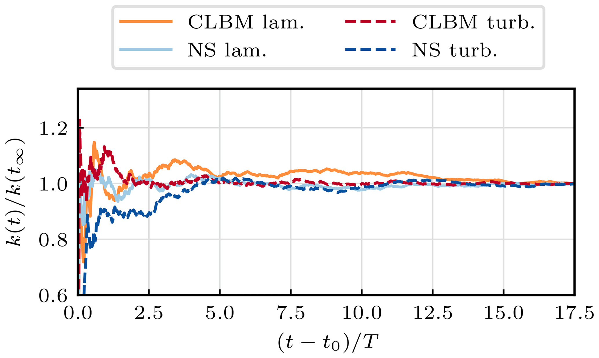
For the evaluation of the ALM we choose one of the most prominent test cases in this context, i.e. the simulation of the NREL 5 MW reference turbine (Jonkman et al., 2009). The mean inflow velocity in all presented cases is u₀=8 m s⁻¹ while the turbine operates at an optimal tip-speed ratio of λ=7.55. With the viscosity of air $\mathit{\nu }=\mathrm{1.78}\times {\mathrm{10}}^{-\mathrm{5}}$ m² s⁻¹ the Reynolds number with respect to the diameter D amounts to $R{e}_{\mathrm{D}}=u_{\mathrm{0}}D/\mathit{\nu }=\mathrm{5.7}\times {\mathrm{10}}^{\mathrm{7}}$ (with D=126 m). The rectangular computational domain spans 6 D in the cross-stream directions and 29 D in the stream-wise direction. The resulting blockage ratio amounts to 2.2 % and was found to have a negligible impact on the code-to-code comparison. For the sake of comparability, the grid is uniformly spaced in the entire domain. The turbine is laterally centred 3 D downstream of the inlet. A schematic of the set-up including the definition of coordinates is given in Fig. 2. All simulations are initially run for t₀=4.39 T, with T being one domain flow-through time. Statistics are subsequently gathered over another 17.52 T. This choice is based on a prior investigation of the convergence of the second-order statistics. Exemplary plots of the temporal development of the turbulent kinetic energy k are given in Fig. 3

Figure 2 Schematic of the case set-up outlining the dimensions of the computational domain, position of the turbine, and definition of coordinates.

Figure 3 Temporal convergence of the turbulent kinetic energy k(t) at x={24 D, 0, 0} normalized by the final value k(t_∞) after 17.52 T averaging. The depicted results refer to the laminar and turbulent inflow cases with a spatial resolution of $\mathrm{\Delta }x=D/\mathrm{32}$ as discussed in Sects. 4 and 5, respectively.

4 Code-to-code comparison in uniform inflow

As a starting point we compare the results obtained with the CLBM to the NS reference in uniform laminar inflow. The simplicity of the case eliminates various uncertainties associated with more complex yet possibly more realistic inflow conditions. Also, it becomes more straightforward to analyse the effect of the numerical scheme on the downstream evolution of the wake and particularly the onset of turbulence as recently discussed by Abkar (2018).

In both solvers we apply the constant Smagorinsky model outlined in Sect. 2.4.1 using a model-constant C_s=0.08, similar to previous studies of the topic (Martínez-Tossas et al., 2018; Deskos et al., 2019). The limiter in the CLBM is set to λ_m=10⁶ and thus practically switched off. Each model is run with three different grid resolutions $\mathrm{\Delta }x=\mathit{\{}D/\mathrm{16}$, D∕24, D∕32}, referring to 4.4, 14.6, and 34.6 million grid points, respectively. This choice of grid resolutions is below values found in fundamental investigations of, for instance, the evolution of tip vortices (Ivanell et al., 2010; Sarmast et al., 2014). Yet, it lies well within the range commonly found in wind farm simulations using the ALM where higher resolutions might be unfeasible, see, e.g. Porté-Agel et al. (2011), Churchfield et al. (2012a), Andersen et al. (2015), or Foti and Duraisamy (2019). Generally, the tip of the actuator line is required not to skip a cell in one time step Δt in order to ensure a continuous coupling of the ALM with the flow field. In NS-based LESs this condition dictates the choice of Δt, resulting in a Courant–Friedrichs–Lewy (CFL) number with respect to u₀ of CFL=0.132. Referring to Troldborg et al. (2010), the CFL number is thus typically lower than required by the LES to obtain time step independence. In LBM simulations the time step is dictated by the Mach number as outlined in Sect. 2.3. A preceding study has shown that the forces determined by the ALM can be significantly more sensitive to the Mach number than the bulk flow depending on the smearing width (Asmuth et al., 2019). Under consideration of this issue we chose Ma=0.1, referring to CFL=0.058 for the CLBM cases. This is obviously well below the value required by the ALM, yet inevitable due to the numerical method.

As for the ALM, the blades in all cases are discretized by 64 points. The smearing width is set to 0.078125 D referring to $\mathit{ϵ}/\mathrm{\Delta }x=\mathit{\{}\mathrm{1.25}$, 1.875, 2.5} for the three different resolutions, respectively.

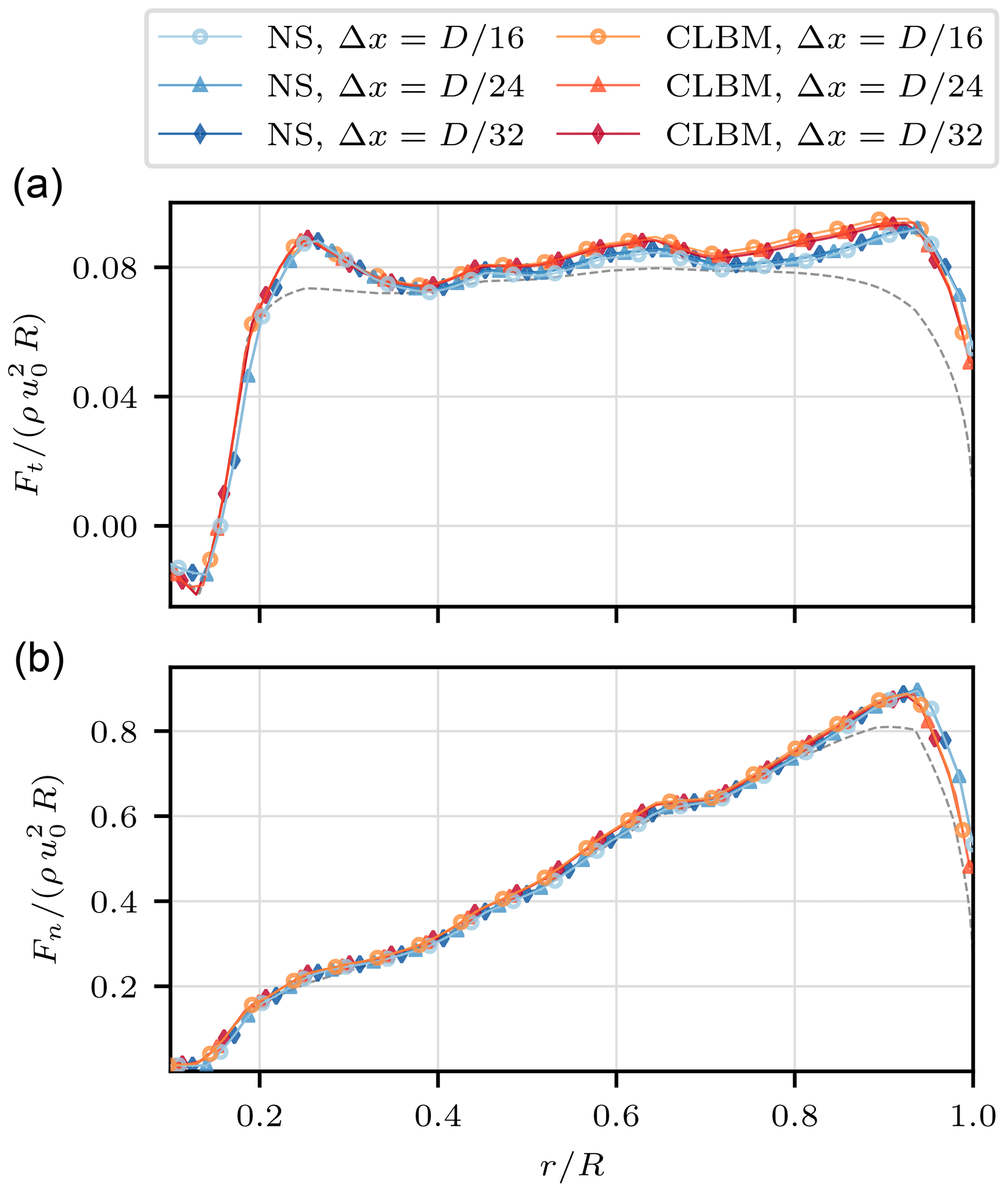
4.1 Blade loads

Results of the simulations for the time-averaged tangential and normal force components of all cases are given in Fig. 4. BEM (blade element momentum) computations following Hansen (2008) are provided as an additional reference. It becomes obvious that the dependency of the blade forces on the grid resolution is small in both numerical approaches. The same holds for the differences between the CLBM and the NS solution, even though these are found to be slightly larger than in the former comparison. The deviations from the BEM reference can be related to the influence of the force smearing as well as the lack of a correction model as discussed by Meyer Forsting et al. (2019). Also, despite the relatively low values for ϵ∕Δx in the cases with $\mathrm{\Delta }x=\mathit{\{}D/\mathrm{16}$, D∕24}, no numerical disturbances were caused by the ALM in the NS simulations. Note that some authors recommend $\mathit{ϵ}/\mathrm{\Delta }\ge \mathrm{2}$ in order to avoid spurious oscillations (Jha et al., 2013; Martínez-Tossas et al., 2015). Here, instabilities were only found for $\mathit{ϵ}/\mathrm{\Delta }\le \mathrm{1}$. The choice of ϵ therefore states a compromise. On the one hand, it ensures numerical stability for the cases with the lowest resolution. On the other hand, ϵ is kept reasonably low with respect to the cases with the highest spatial resolution. Note that unnecessarily large smearing widths would imply larger deviations from the underlying lifting line theory and are therefore undesirable (Martínez-Tossas and Meneveau, 2019). In summary, and in line with other similar code-to-code comparisons (Sarlak, 2014; Sarlak et al., 2015b; Martínez-Tossas et al., 2018), it can be concluded that the agreement in the blade forces is sufficient to facilitate a wake comparison with focus on the behaviour of the bulk scheme. Alternatively, it could be considered to prescribe the body forces along the actuator lines for the sake of a pure wake comparison. Yet, as this study aims for a comparison of the ALM as a whole, including the interaction of the aerodynamic model with the flow solver, this approach is not pursued here.

Figure 4 Mean tangential force F_t (a) and normal force F_n (b) along the actuator line. For the sake of visibility, markers are only shown for every third data point. The grey dashed line marks the BEM reference by Hansen (2008).

4.2 Wake characteristics

Firstly, we compare the time-averaged cross-stream velocity profiles, given in Fig. 5. Furthermore, Fig. 6 provides a direct comparison of the depicted velocity components of the two numerical approaches at each reference grid resolution by means of the L²-relative error along the profile, i.e.

$$\begin{array}{}\text{(19)}& L^{\mathrm{2}}\left(\mathit{\varphi }\right)=\sqrt{{\displaystyle \frac{\sum _{k=\mathrm{1}}^{n_z}{\left({\mathit{\varphi }}_{\mathrm{CLBM}}\left(z_k\right)-{\mathit{\varphi }}_{\mathrm{NS}}\left(z_k\right)\right)}^{\mathrm{2}}}{\sum _{k=\mathrm{1}}^{n_z}{\mathit{\varphi }}_{\mathrm{NS}}{\left(z_k\right)}^{\mathrm{2}}}}},\end{array}$$

where $\mathit{\varphi }=\mathit{\{}\stackrel{\mathrm{‾}}{u}$, $\stackrel{\mathrm{‾}}{v}\mathit{\}}$ and n_z is the number of sample points along the profile.

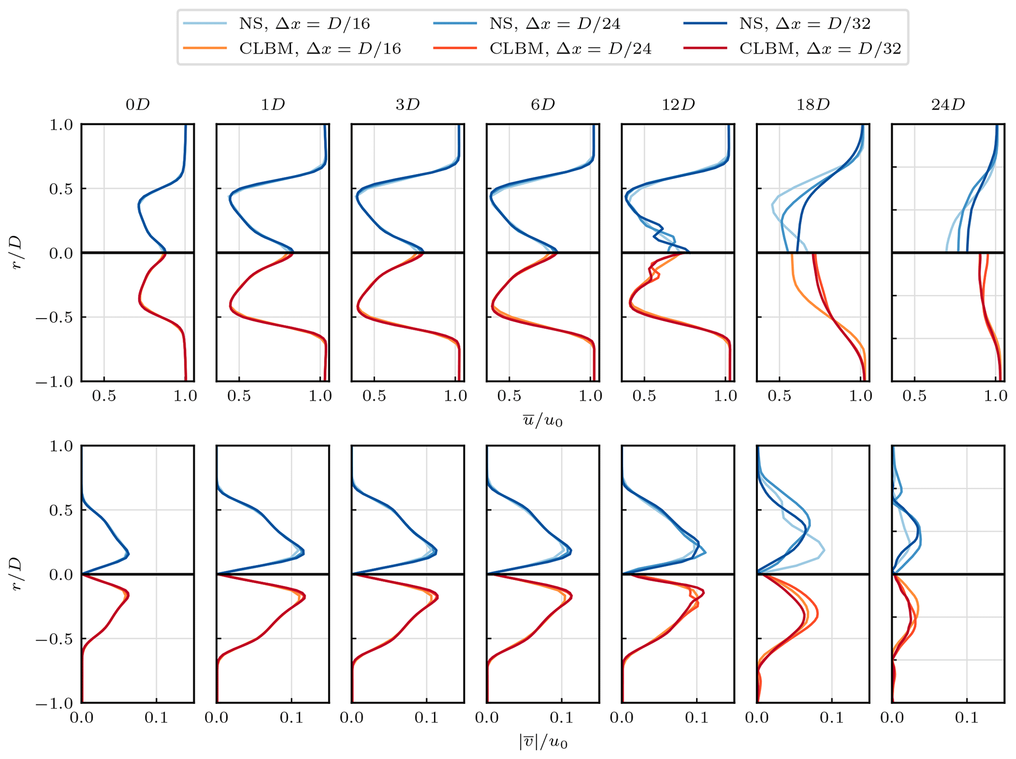
Figure 5 Cross-stream profiles of the mean stream-wise velocity $\stackrel{\mathrm{‾}}{u}$ (top) and tangential velocity $\stackrel{\mathrm{‾}}{v}$ (bottom) of the CLBM compared to the NS reference cases at different downstream positions.

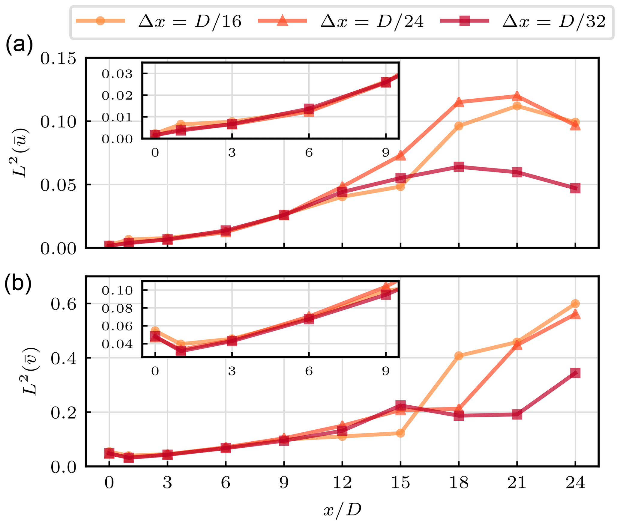
Figure 6 Relative difference (L²-relative error norm) between the NS and CLBM solution in $\stackrel{\mathrm{‾}}{u}$ (a) and $\stackrel{\mathrm{‾}}{v}$ (b) at each referring spatial resolution along velocity profiles as given in Fig. 5.

It can be seen that the two numerical approaches are in good agreement in the near wake of the turbine. Up until x=3 D, differences in $\stackrel{\mathrm{‾}}{u}$ amount to less than 1 % while increasing to ∼3 % at x=9 D. The differences in the tangential velocity component $\stackrel{\mathrm{‾}}{v}$ are found to be somewhat higher with ∼5 % for x≤3 D increasing to ∼10 % at x=9 D. The latter can be related to the fact that we also find higher differences in the tangential than in the normal force component as shown in Fig. 4

In the near-wake region discussed here, viscous effects usually only play a minor role. Among others, this is shown in a small wake recovery. Also, the rotational velocity does not change significantly. The wake is thus mostly governed by the inviscid flow solution (Troldborg, 2008; Troldborg et al., 2010). Both the NS and the CLBM approaches recover the Euler equations at the same order of accuracy. A similar numerical behaviour in this part of the wake should therefore be expected (assuming comparability of all other aspects like boundary conditions and the implementation of the ALM). In light of the motivation for this comparison, these results can thus be appreciated.

Further downstream (x>9 D) differences between all compared cases increase significantly. Generally, the vortex sheet of the near wake starts to meander and eventually breaks down as the wake transitions to a fully turbulent state. An impression thereof is provided in Fig. 7, showing the downstream evolution of the wake in terms of the contour plots of the instantaneous stream-wise velocity. After the onset of turbulence the wake starts to recover more rapidly while the turbulence slowly decays. Differences in the velocity in the far wake between both the two numerical approaches and the respective grid resolutions can therefore be related to different downstream positions of the points of transition.

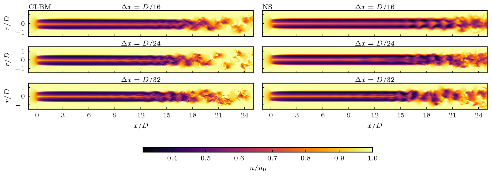
Figure 7 Contour plots of the instantaneous stream-wise velocity u in the central stream-wise plane at different spatial resolutions (top to bottom panels) with the CLBM (left panels) and NS (right panels).

More quantitatively, the breakdown of the wake can be observed by means of a drastic increase in the turbulence intensity Ti as depicted in Fig. 8. It shows that the turbulence intensity in all CLBM cases lies at a similar magnitude in the near wake. At the same time it is notably higher than in the NS cases at the same downstream position. Downstream of x=6 D it can be seen that Ti increases faster with downstream distance the higher the spatial resolution. Also, it increases earlier in the CLBM than in the NS solutions. In addition to Fig. 8 this process is illustrated in Fig. 9 by means of the stream-wise evolution of Ti at a radial position of $r/D=\mathrm{0.625}$. It clearly shows the faster increase in Ti at higher spatial resolutions as well as a downstream shift of the build-up in the NS cases.

Figure 8 Cross-stream profiles of the turbulence intensity $\text{Ti}=\frac{\mathrm{1}}{u_{\mathrm{0}}}\sqrt{\frac{\mathrm{1}}{\mathrm{3}}\stackrel{\mathrm{‾}}{u_i^{\prime }{u}_i^{\prime }}}$ of the CLBM compared to the NS reference cases. Please note the log scale on the abscissa. Gaps in the line plots (at x=3 D) refer to regions of negligible Ti. For the legend, see Fig. 5.

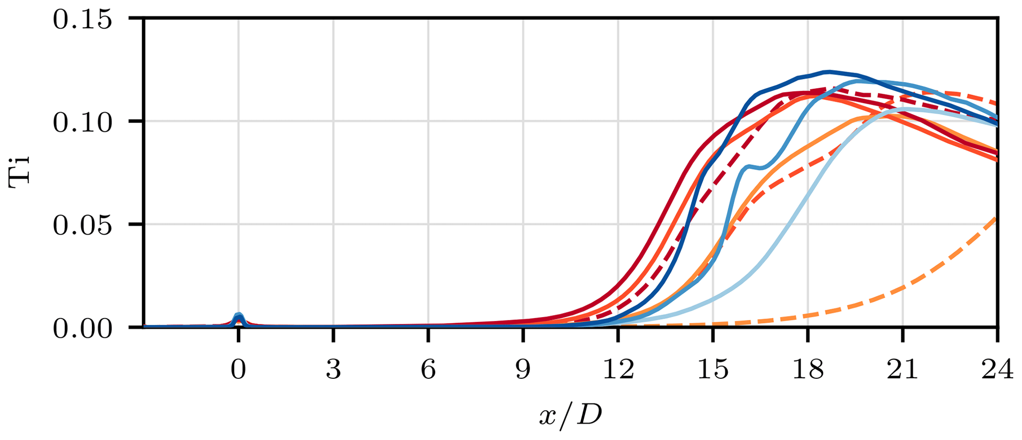
Figure 9 Stream-wise evolution of the turbulence intensity Ti at $r/D=\mathrm{0.625}$ in the CLBM and NS cases. For the legend, see Fig. 5. Additional dashed lines refer to AllOne CLBM results. These briefly illustrate the impact of the increased order of accuracy when using the parameterized relaxation rates of the CLBM on the wake transition.

The mechanism of the transition of wind turbine wakes has been extensively described based on ALM simulations; see, e.g. Sarmast et al. (2014). Fundamental studies thereof do, however, mostly use higher spatial resolutions in order to resolve distinct tip vortices. With the resolutions and smearing width used here the wake rather resembles a vortex sheet similarly to actuator disc simulations. To the authors' knowledge only Martínez-Tossas et al. (2018) briefly described the transition process of wakes of such low-resolution ALM. In their discussion of a similar code-to-code comparison, the authors argue that small perturbations at high wave numbers eventually trigger the transition of the wake. Schemes with lower numerical diffusivity (pseudo-spectral approaches in that study) generally dampen those perturbations less than more diffusive lower-order schemes (referring to second-order collocated finite-volume discretizations, equivalent to the NS reference used here) and thus show a faster growth of turbulence. The same interpretation can indeed be applied to the results shown here. As described in Sect. 2, the parametrization of the relaxation rates results in a scheme with fourth-order accuracy in diffusion as opposed to the second-order accuracy of the NS finite-volume scheme. At this point we shall briefly comment on the second-order accurate AllOne CLBM mentioned earlier (Sect. 2). In fact, using this version of the CLBM shifts the transition further downstream when compared to the parameterized CLBM; see Fig. 9. This generally corroborates the aforementioned discussion on the effect of the numerical diffusivity. As for this case, the scheme even appears to be more diffusive than the NS solution. Be aware, however, that the diffusivity of the AllOne CLBM also strongly depends on the Mach number (as opposed the parameterized approach). Nevertheless, a further analysis of the AllOne CLBM is not the focus of this study and is omitted here for the sake of brevity.

As a last aspect we analyse the one-point turbulence kinetic energy spectra. The spectra shown in Fig. 10 represent the average of 16 points in the respective cross-sectional plane at a radial position of $r/D=\mathrm{0.625}$. For additional smoothing the Welch method was applied at each point with non-overlapping time intervals of a 15th of the overall sampling period.

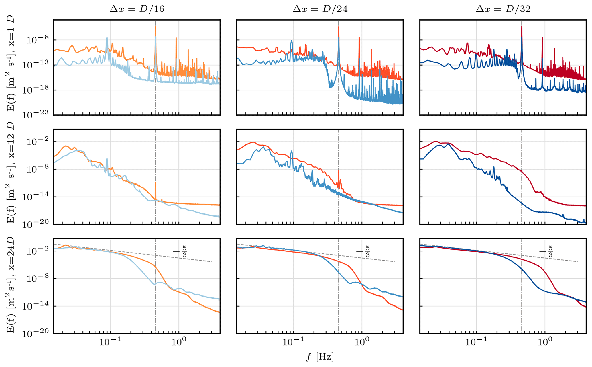
Figure 10 One-point turbulent kinetic energy spectra in the near (x=1 D, top) and far wake (x=12 D, middle; x=24 D, bottom) at increasing spatial resolution from left to right. The vertical dashed–dotted line marks the blade-passing frequency $f_{\mathrm{B}}=\left(\mathrm{3}{u}_{\mathrm{0}}\mathit{\lambda }\right)/\left(\mathit{\pi }D\right)=\mathrm{0.458}$ Hz. Mind the change of scale on the y axis between the first and second rows of subplots. For the legend, see Fig. 5.

The energy content in the near wake (x=1 D) is expectedly small when compared to the far wake where the vortex sheet has broken down in most of the shown cases. The energy level across most frequencies is indeed low enough to be related to numerical noise, making further interpretation unnecessary. The only distinct feature at x=1 D are notable peaks at the blade-passing frequency f_B and its higher harmonics. These are found in all presented cases, yet are generally slightly smaller in the NS solutions. This signature at f_B was recently described by Nathan et al. (2018) but using twice as many grid points per diameter when compared to the highest resolution shown here. It can thus be appreciated that this transient feature of the ALM remains traceable down to resolutions of $\mathrm{\Delta }x=D/\mathrm{16}$.

At x=12 D a pre-transition wake meandering can be seen. The occurrence of this feature is not as confined to a single frequency as the aforementioned blade-passing frequency. Yet, an increased energy level in a frequency band around f_m≈0.025 Hz (and its higher harmonics) can be observed in all cases. It was illustrated in Fig. 7 that the meandering starts to occur at different positions downstream depending on the resolution and numerical approach. It then steadily increases until the wake becomes fully turbulent. The amplitudes at f_m therefore differ depending on how far upstream the meandering started to build up. Also, it again shows that the meandering and subsequent transition occurs earlier in the CLBM cases. Additionally, the signature of the blade passage is still visible in the lower-resolution CLBM cases. This is not the case for the NS reference, despite the smaller meandering at this downstream position. In line with the observations made earlier, this aspect might relate to a higher numerical dissipation of the NS scheme.

Further downstream at x=24 D the wake is fully turbulent in all CLBM cases, characterized by a sub-inertial range with a typical $-\mathrm{5}/\mathrm{3}$ slope. This is also the case for the NS solution with $\mathrm{\Delta }x=D/\mathrm{32}$. Here, however, the meandering is still more visible due to the later start of the transition of the wake. Also, when comparing both approaches at the highest spatial resolution (bottom right in Fig. 7) it shows that the sub-inertial range of the CLBM approach reaches to higher frequencies. In accordance with that, it appears that the CLBM does indeed resolve smaller turbulent structures, as shown in the contour plot of the Q criterion (Fig. 11).

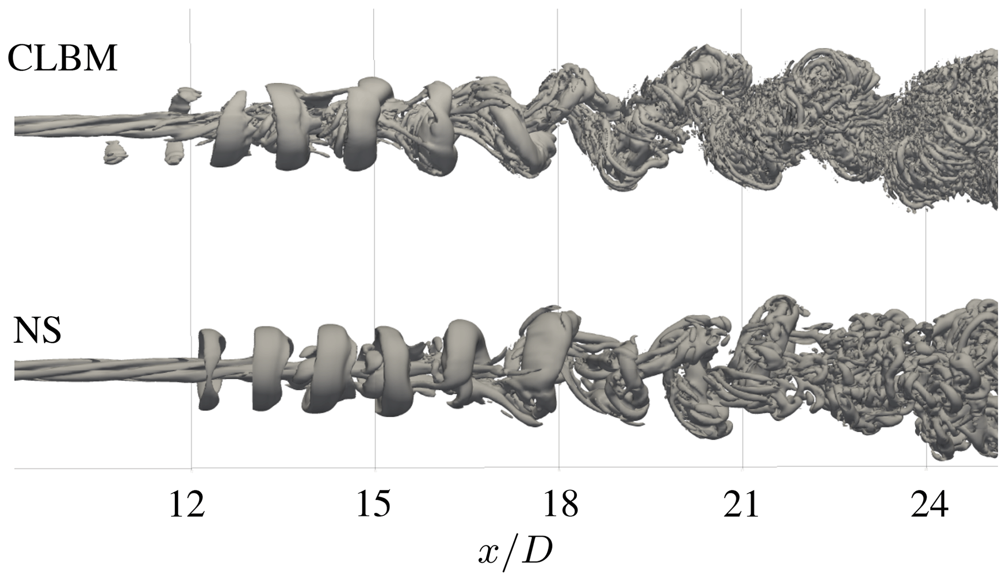
Figure 11 Rendering of the instantaneous contours of the Q criterion (Q=0.0005) in the far wake with the CLBM and NS with $\mathrm{\Delta }x=D/\mathrm{32}$.

5 Code-to-code comparison in turbulent inflow

Laminar inflow cases allow for a good comparison of fundamental numerical aspects as discussed in Sect. 4. Nevertheless, the case itself remains rather academic as atmospheric inflows are mostly turbulent. Furthermore, Sect. 4 has shown that a direct comparison of the far wake can be difficult due to the different downstream positions of the laminar-to-turbulent transition of the wake. A turbulent inflow generally accelerates the transition while reducing the dependency of the point of transition on the numerical diffusivity of the scheme. A complementing comparison in turbulent inflow will therefore be presented in the following. For the sake of brevity we limit the discussion to cases with the highest spatial resolution $\mathrm{\Delta }x=D/\mathrm{32}$. Apart from the introduction of turbulence at the inlet, both numerical set-ups remain unchanged. Also note that the mean resulting blade loads exhibit no notable difference towards the laminar inflow case. Additional discussion beyond Sect. 4.1 is therefore omitted.

5.1 Synthetic turbulence generation at the inlet

At the inlet we prescribe homogeneous isotropic turbulence (HIT) based on the von Kármán energy spectrum. The three-dimensional field of velocity fluctuations is generated based on the method developed by Mann (1998) using the open-source code TuGen by Gilling (2009). As we are only interested in HIT the model's shear parameter Γ is set to zero. The length scale of the spectral velocity tensor is chosen as L=40 m = 0.317 D. The mean turbulence intensity is scaled via the coefficient $\mathit{\alpha }{\mathit{ϵ}}^{\mathrm{2}/\mathrm{3}}=\mathrm{0.01}$. The resulting Ti of the turbulence field measures Ti=0.028. The length of the turbulence field in the stream-wise direction measures 24 576 m. Following Taylor's frozen turbulence hypothesis the field is advected with u₀. The turbulence field is consequently recycled after 6.72 domain flow-through times. The lateral dimensions of the field are set to 1536 m (referring to 12.19 D). Since we only use a cross section of 6 D×6 D, we ensure zero correlation of the velocity fluctuations between the lateral boundaries of the domain. The spatial resolution of the field is 8192 grid points in the stream-wise direction and 64 grid points in the lateral directions. In both numerical approaches the velocity fluctuation is superimposed with the mean inflow velocity u₀ and applied at the inlet.

Figure 12 compares the stream-wise evolution of the turbulence intensity at hub height without ALM. At the inlet we find a turbulence intensity of 2.3 % in both approaches, which is slightly lower than the one of the synthetic turbulence field. Such discrepancies have been discussed earlier and are commonly counteracted by scaling a given turbulence field if a desired turbulence intensity is to be matched (see, e.g. Olivares-Espinosa et al., 2018; van der Laan et al., 2019). Some possible explanations of this issue are given by Gilling and Sørensen (2011). Among others, they argue that the discrete representation of the otherwise continuous turbulence field can lead to noticeable discontinuities when being differentiated with low-order schemes. Directly after the inlet the NS solution shows a small increase in Ti followed by a continuous decay throughout the entire domain. The turbulence intensity in the CLBM solution initially drops behind the inlet. However, the subsequent decay up until x=12 D is lower than in the NS solution. The decay rates of the two approaches seem to align only at the far end of the domain. As a result, the turbulence intensity at the turbine position differs by ΔTi=0.0005 while the maximum difference further downstream amounts to ΔTi=0.0027. A detailed analysis of the rather fundamental aspects related to these discrepancies goes beyond the scope of this paper. After all, the observed differences remain small enough not to be significant when compared to the turbulence related to the wake flow, as shown later.

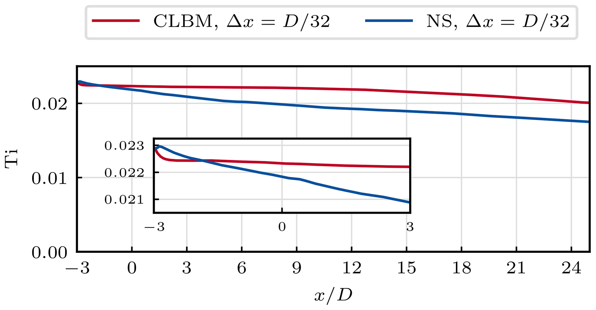
Figure 12 Stream-wise evolution of the turbulence intensity Ti without ALM. Each data point Ti(x) refers to the spatial mean of 64 points in the cross-stream direction z with $-D\le z\le D$.

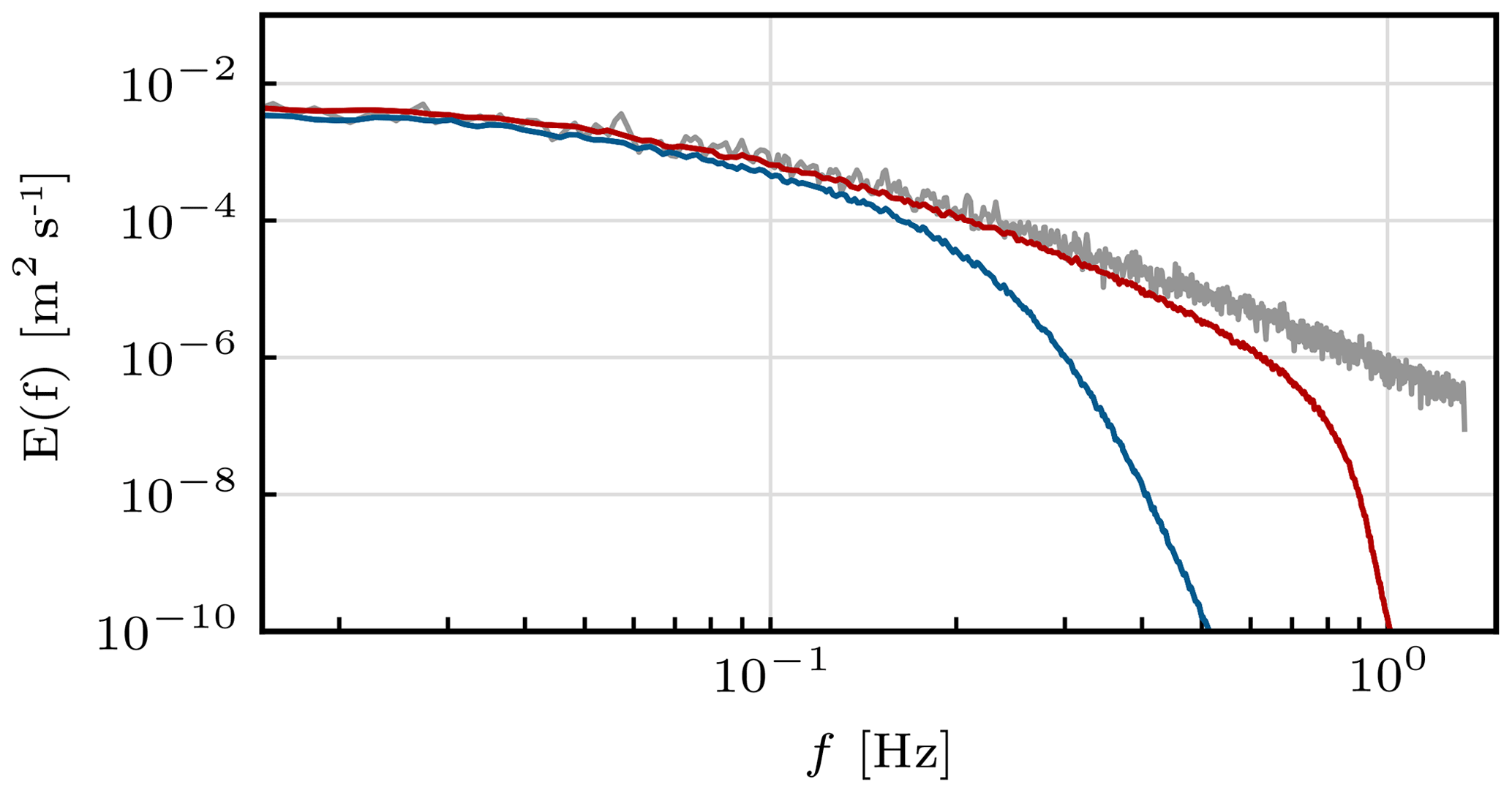
Figure 13 depicts the spectra of the turbulent kinetic energy at the turbine position. Chiefly, it shows that the CLBM exhibits a sub-inertial range extending to higher frequencies than the NS solution, similarly to the far-wake turbulence found in laminar inflow (see Fig. 10).

Figure 13 One-point turbulent kinetic energy spectra at the turbine position (x=0 D) without ALM. The spectrum of the synthetic inlet turbulence is given in grey. For the legend, see Fig. 12.

5.2 Wake characteristics

Analogously to Sect. 4, we firstly compare the cross-stream profiles of the mean velocity in Fig. 14. In the stream-wise velocity component $\stackrel{\mathrm{‾}}{u}$ we find an excellent agreement of the two solutions. When compared to the laminar cases discussed before, this not only applies to the near wake but also the entire domain. The difference in $\stackrel{\mathrm{‾}}{u}$ between the cross-stream profiles of the two approaches for x≤12 D amounts to less than 1 % in terms of the L²-relative error norm as shown in Fig. 15. While steadily increasing with downstream distance, the maximum discrepancy measures 1.6 % at x=24 D. Be aware that the laminar inflow cases only exhibited similar agreements in the near wake.

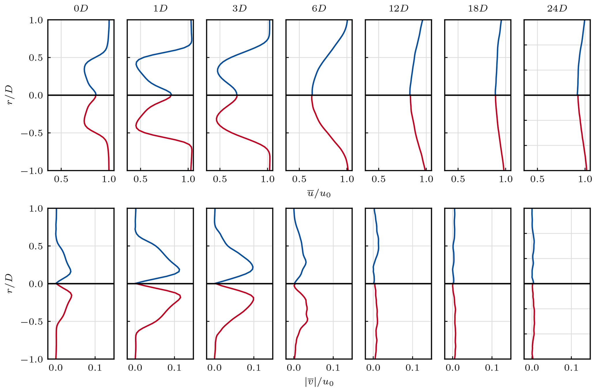
Figure 14 Cross-stream profiles of the mean stream-wise velocity $\stackrel{\mathrm{‾}}{u}$ (top panels) and tangential velocity $\stackrel{\mathrm{‾}}{v}$ (bottom panels) of the CLBM and NS references in turbulent inflow. For the legend, see Fig. 12.

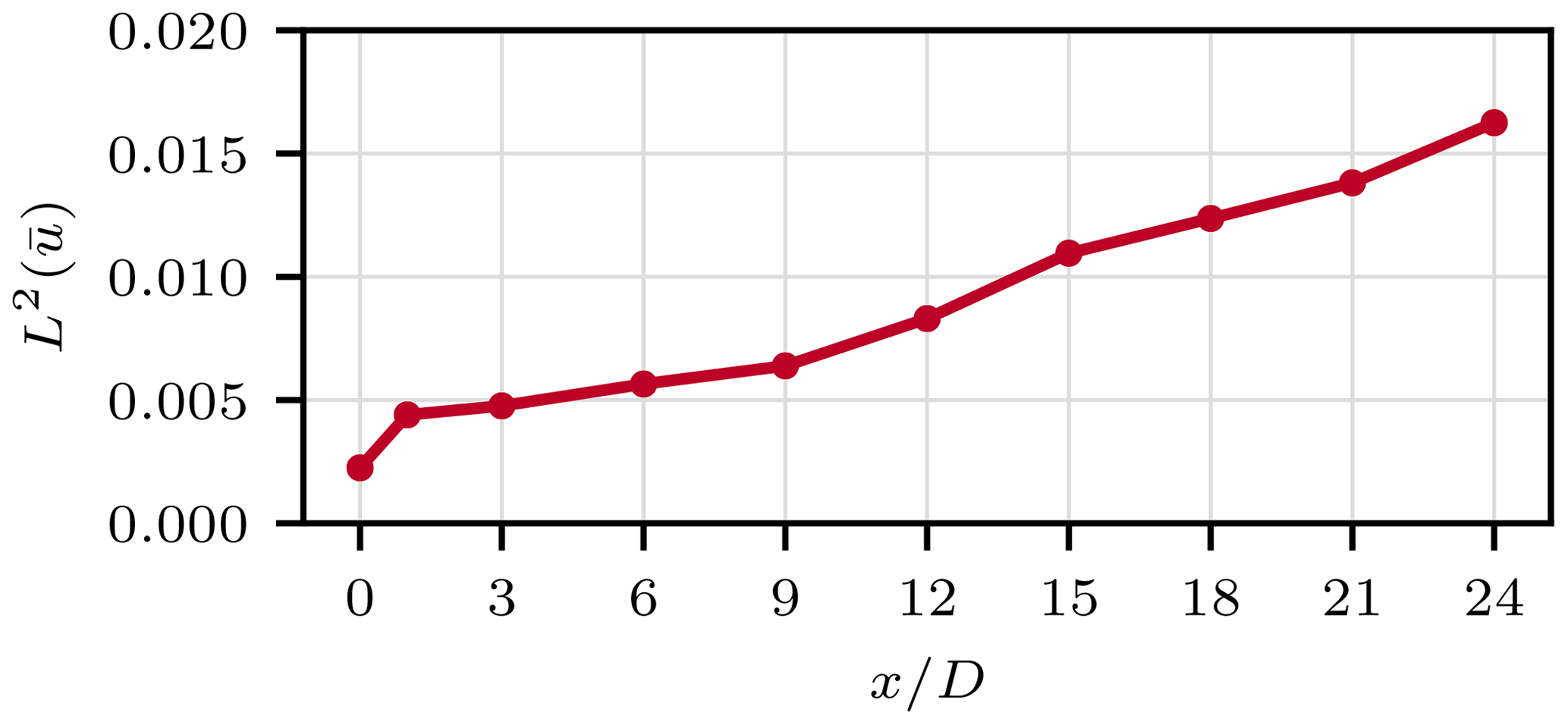
Figure 15 Relative difference (L²-relative error norm) between the NS and CLBM solution in $\stackrel{\mathrm{‾}}{u}$ in turbulent inflow along velocity profiles as given in Fig. 14.

Profiles of the turbulence intensity are shown in Fig. 16. Similarly to the velocity, differences between the CLBM and NS solutions are small. Most importantly, it can be observed that the transition of the wake is triggered at very similar downstream positions. This also explains the significantly better agreement in the velocity. After all, most differences observed in laminar inflow are related to the different downstream positions of the laminar-to-turbulent transition.

Figure 16 Cross-stream profiles of the turbulence intensity Ti of the CLBM and NS references in turbulent inflow. For the legend, see Fig. 12.

In the case discussed here the transition is dominated by instabilities introduced by the ambient turbulence. As opposed to the transition in laminar inflow, the impact of the dissipative characteristics of the numerical scheme here appears to be subordinate, if not negligible. Without imposed turbulence, perturbations triggering the transition grow within the wake itself starting from infinitesimal magnitudes as outlined in Sect. 4. Hence, the transition mainly depends on the growth of such perturbations and eventually the point where they reach a critical magnitude. Consequently, the transition is increasingly delayed the higher this growth is dampened by the numerical dissipation. In contrast, the imposed turbulence states a finite-size perturbation that affects the wake immediately from the rotor plane downstream independent of the numerical scheme and its dissipative properties. Similar observations in turbulent inflow have been discussed by Martínez-Tossas et al. (2018). Among others, the study assessed the impact of the Smagorinsky parameter C_s on wake flows in laminar and turbulent inflow. Altering C_s effectively also results in different overall diffusivities.

The spectra of the turbulent kinetic energy at three different downstream positions are provided in Fig. 17. As in the laminar case, a distinct peak at the blade-passing frequency f_B and its higher harmonics can be observed in both approaches in the near wake (x=1 D). From the velocity profiles in Fig. 14 it can be inferred that the transition of the wake occurs between x=3 and x=6 D, characterized by the change from a typical near-wake to a far-wake Gaussian profile. In the spectra this is reflected by an overall increase in the energy level across all resolved frequencies. Also, the signature of f_B is no longer visible. Moving further downstream (x=18 D) the overall turbulent kinetic energy decreases due to the continuous decay of both ambient and far-wake turbulence. When compared to the previous position, the energy content at smaller scales increases slightly relative to the larger scales. The latter relates to the continuous breakdown of the turbulent structures of the wake along the energy cascade. The relative energy increase at higher frequencies appears to be more pronounced in the CLBM solution. Again, this might relate to the higher dissipation found in the NS solver inducing an earlier cut-off in the sub-inertial range as discussed earlier.

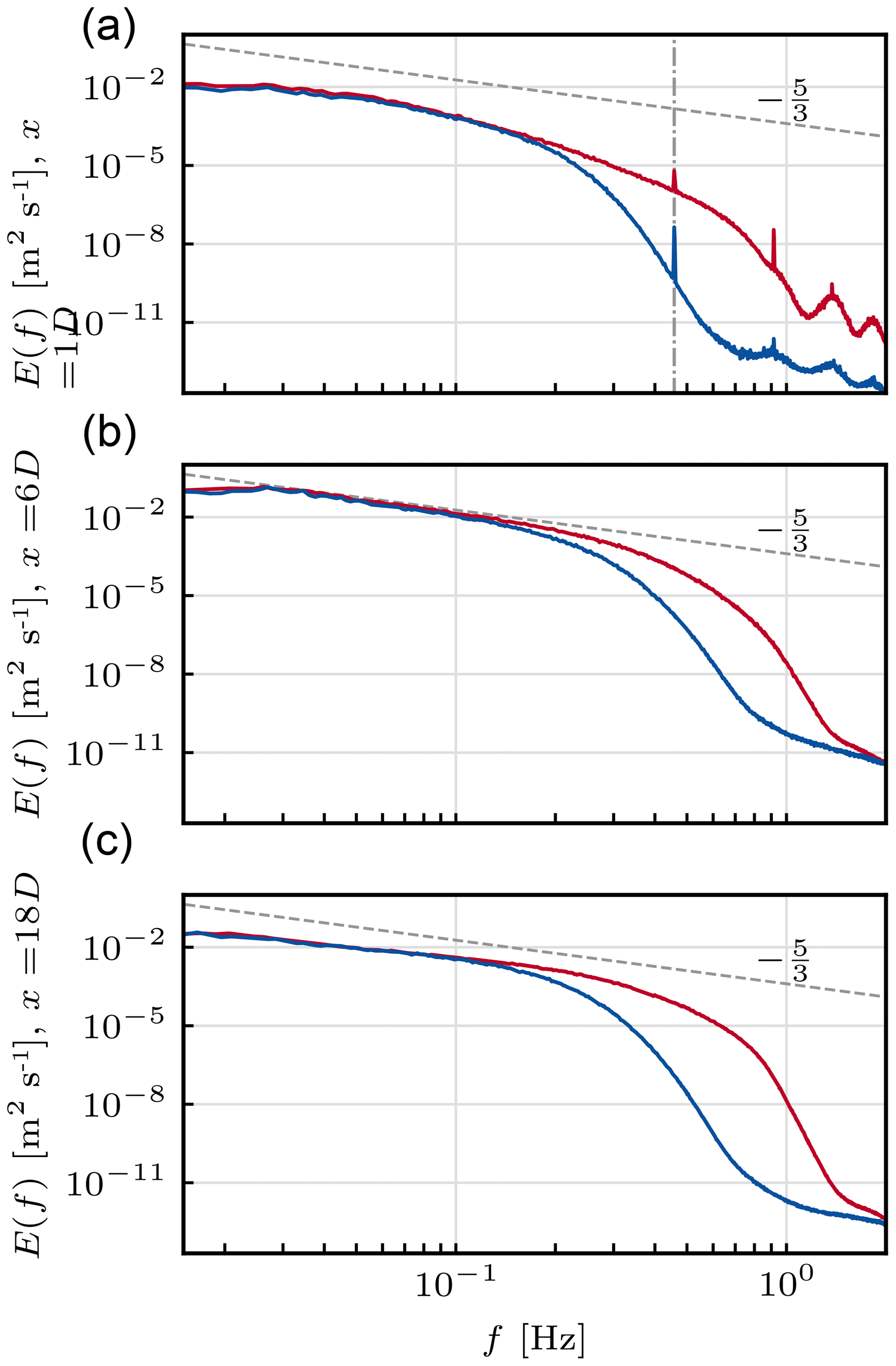
Figure 17 One-point turbulent kinetic energy spectra in the near wake (x=1 D, a), transition region (x=6 D, b), and far wake (x=18 D, c) in turbulent inflow. Vertical dashed–dotted line marks the blade-passing frequency f_B. For the legend, see Fig. 12.

Lastly, we shall comment on the small differences in the ambient turbulence shown earlier. Based on the above elaborations one might expect a more notable impact on the wake characteristics. With regards to this we refer to the study by Sørensen et al. (2015). Based on a more extensive investigation of the impact of ambient turbulence on the length of the near wake, the authors present an empirical description of the problem. In summary, they find that the distance of the transition point to the turbine l is a function of ln(Ti). Following this the relative difference in l can thus be expected to be $\mathcal{O}(\mathrm{1}-\ln ({\mathrm{Ti}}_{\mathrm{NS}})/\ln ({\mathrm{Ti}}_{\mathrm{CLBM}}\left)\right)=\mathcal{O}\left({\mathrm{10}}^{-\mathrm{3}}\right)$ with the given inflows, lying well within the range of the differences observed here.

6 Impact of the third-order cumulant limiter

A further aspect of the CLBM to be discussed is the impact of the limiter of the third-order cumulants described in Eq. (15). The main motivation behind the limiter is to provide a damping of high-wave-number perturbations in the CLBM in order to ensure numerical stability. Geier et al. (2017b) showed theoretically and by means of a decaying shear-wave and Taylor–Green vortex that the use of the limiter does not affect the asymptotic order of accuracy of the scheme. Investigations of the effects of the limiter in more applied high-Reynolds-number cases are, however, not available to date. Geier et al. (2017a) and Lenz et al. (2019) presented applications of the parameterized CLBM, yet both did not touch upon the topic discussed here. Then again Pasquali et al. (2017) state that they chose suitable values for λ_m manually, close to the stability limit and case-dependent. Both the effect of λ_m on turbulent flows and criteria to choose adequate values thus remain open questions. At the same time, some authors refer to the parameterized CLBM and also the AllOne as implicit LESs (see Far et al., 2017; Lenz et al., 2019; Nishimura et al., 2019). However, the latter is solely supported by the fact that the CLBM remains numerically stable in under-resolved turbulent flows without explicit turbulence models (as opposed to many other LBM collision operators). To the authors' knowledge, a full understanding of the dissipation behaviour associated with the limiter (or the AllOne), especially in under-resolved flows, is still lacking. This again, though, would be clearly required to fully replace an explicit SGS model.

In the code-to-code comparison the limiter was practically switched off for the sake of comparison. Hence, numerical stability was also solely provided by the Smagorinsky model. Motivated by the lack of experience with the use of the limiter, we provide a brief investigation of the characteristics of the wake in comparison to the case with the Smagorinsky model used in Sect. 4. For the sake of brevity we only discuss a resolution of $\mathrm{\Delta }x=D/\mathrm{32}$. Three values of λ_m are investigated ranging from 10⁰ to 10⁻². The former value is the largest possible to ensure numerical stability.

Contour plots of the mean stream-wise velocity and turbulence intensity are shown in Fig. 18. While the mean velocity in the region close to the turbine is almost unaffected by the choice of λ_m, the evolution of the turbulence intensity and ultimately the point of transition change drastically. With λ_m=10⁰, Ti grows significantly, closely behind the turbine. At only 3 D downstream the wake is highly turbulent. With ${\mathit{\lambda }}_{\mathrm{m}}={\mathrm{10}}^{-\mathrm{1}}$ the wake characteristics only change marginally. Increasing λ_m from 10⁻¹ to 10⁻², however, delays the transition considerably. This implicitly shows that the order of magnitude of the third-order cumulants in crucial regions of the wake lies within this range, which can be deduced from Eq. (15). When choosing ${\mathit{\lambda }}_{\mathrm{m}}={\mathrm{10}}^{-\mathrm{2}}$ the limiter dampens the third-order cumulants considerably when compared to the optimized relaxation rates. Moreover, the far-wake distribution of Ti more closely resembles that of the Smagorinsky case than with lower λ_m. Turbulent perturbations of the wake do, however, grow over a longer fetch than in the Smagorinsky case, starting in the near wake. Moreover, it should be noted that increasing λ_m also increases the amplitude of small-scale fluctuations in the ambient flow field. Among others, these are likely to be related to acoustic reflections of small-scale turbulence on the domain boundaries and/or spurious numerical oscillations. Partially, these can be seen in the Ti contour plots (Fig. 18) upstream of the turbine for the two higher λ_m values. More specifically, 1 D upstream of the turbine, we find $\mathrm{Ti}=\mathcal{O}({\mathrm{10}}^{-\mathrm{4}}$) for λ_m=10⁰. In comparison, the CLBM case with the Smagorinsky model as well as the NS reference discussed earlier exhibit a magnitude that is 2 and 3 orders of magnitude lower, respectively. Referring to the discussions of tip-vortex stability by Ivanell et al. (2010) or Sørensen et al. (2015), an effect thereof on the breakdown of the wake can not be ruled out. Unfortunately, most studies similar to the one presented here did not comment on this topic. Deskos et al. (2019), on the other hand, found that the mutual inductance of tip vortices can be severely disturbed if the diffusivity of the scheme is too low.

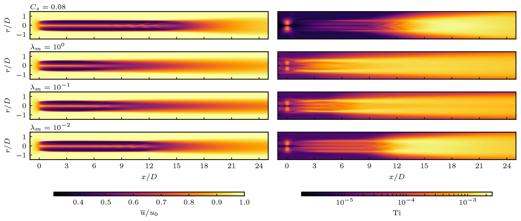
Figure 18 Contour plots of the mean stream-wise velocity $\stackrel{\mathrm{‾}}{u}$ (left panels) and turbulence intensity Ti (right panels) in the central stream-wise plane in uniform inflow. Top panels: Smagorinsky model with a practically switched-off limiter, i.e. ${\mathit{\lambda }}_{\mathrm{m}}={\mathrm{10}}^{-\mathrm{6}}$ (as described in Sect. 4). Second to last row panels: no explicit turbulence model with different values of the third-order cumulant limiter.

The presented case study underlines that the impact of the limiter is sufficiently large to arbitrarily tune the scheme's dissipativity over a wide range. Hence, the choice of the limiter in underresolved flows is by no means irrelevant despite the negligible influence on the asymptotic order of accuracy. On the other hand, the limiter conceivably states a measure to achieve implicit LES characteristics with the CLBM. As mentioned earlier, though, this clearly requires a more systematic understanding and subsequent tuning. Without the latter, the use of classical well-documented SGS models might remain more practical. Ultimately, they also provide numerical stability while choices for model parameters can build on well-documented experience.

7 Computational performance

We initially outlined that the main motivation for the use of the LBM in this context is the method's superior computational performance. Nevertheless, a detailed discussion is not the focus of this paper. For further details on this topic we refer to our previous study (Asmuth et al., 2019) as well as numerous other publications; see, for instance, Schönherr et al. (2011), Obrecht et al. (2013), Januszewski and Kostur (2014), Hong et al. (2016), or Onodera et al. (2018). In brief, we shall remark that all simulations with the CLBM ran with an average of 1050 MNUPS (million node updates per second). A similar single-GPU performance on uniform grids was recently reported by Lenz et al. (2019). For the cases discussed in this study this refers to a wall time of 524 s per domain flow-through time on a single Nvidia RTX 2080 Ti on a local workstation. Putting this into perspective, the wall time per flow-through time of the NS case amounts to 5028 s. The latter ran on 1044 CPU cores (Intel Xeon Gold 6130) and thus amounts to 1463 CPUh. A last interesting aspect to remark upon is the ratio of simulated real time to computation time $r_{\mathrm{r}\mathrm{2}\mathrm{c}}=\mathrm{\Delta }{t}_{\mathrm{real}}/\mathrm{\Delta }{t}_{\mathrm{comp}}$. The topic was recently addressed in the context of urban flows (Onodera and Idomura, 2018; Lenz et al., 2019) as well as for atmospheric boundary layer flows and wind energy applications (Bauweraerts and Meyers, 2019). A ratio of r_r2c>1 would enable the use of LES for real-time forecasts of, for example, urban micro-climates or wind farm performance and loads. For this specific LBM case we obtain r_r2c=0.902. For the NS approach we get r_r2c=0.094. Despite this obviously only being a case study, real-time LES of wind farms with affordable hardware appears to be possible.

8 Conclusions

The cumulant lattice Boltzmann method was applied to simulate the wake of a single wind turbine in both laminar and turbulent inflow. The turbine was represented by the actuator line model. The presented model was compared against a well-established finite-volume Navier–Stokes solver. It was shown that the cumulant lattice Boltzmann implementation of the actuator line model yields comparable first- and second-order statistics of the wake. More specifically, a very good agreement of the two numerical approaches was found in the near wake in laminar inflow, with differences amounting to less than 3 % in terms of the wake deficit. Larger discrepancies occurring in the far-wake were attributed to differences in the point of transition. These in turn could be related to the different numerical diffusivities of the schemes, building onto previous similar code-to-code comparisons (Sarlak, 2014; Sarlak et al., 2016; Martínez-Tossas et al., 2018). On the other hand, the comparison in turbulent inflow showed an excellent agreement of the two solutions in both the near and far wake. Here, differences in the numerical schemes were found to be subordinate as the wake characteristics were dominated by the imposed turbulence. The latter manifested in differences in the wake deficit of less than 1 % in large parts of the domain.

An additional case study investigated the impact of the third-order cumulant limiter in laminar inflow. It was shown that the choice of the limiter largely affects the dissipativity of the scheme. Likewise, the tunability of this dampening characteristic clearly shows the potential to be used in a more systematic way and might be exploited as an implicit LES feature. Yet, this requires further fundamental investigations in order to understand and calibrate it or even develop procedures to determine optimal values dynamically. As of now, the use of explicit eddy-viscosity SGS models thus appears more practical despite a small computational overhead.

As for future applications of the lattice Boltzmann method to more realistic wind-power-related flow cases, the following conclusions can be drawn. First and foremost, the presented study underlines the suitability of the cumulant lattice Boltzmann method for the simulation of highly turbulent engineering flows. The crucial advantage over other collision operators is the superior numerical stability of the method. No other collision operator initially tested in this study was found to be sufficiently robust using the given grid resolutions. The tested single- and multiple-relaxation-time models therefore do not appear suitable for LES of entire wind farms where higher spatial resolutions are not feasible and viscosities on the lattice scale consequently small. The advantages of the parameterized cumulant clearly render it a preferable collision model for wind turbine simulations and presumably other atmospheric flows. Application-oriented studies of the model are so far limited to this work and the recent study by Lenz et al. (2019). Further investigations of the model are therefore clearly required. This applies especially to wall-bounded turbulent flows like atmospheric boundary layers that require the use of wall models. When compared to Navier–Stokes-based LES, the experience with wall models in the LBM in general is limited to only a handful of studies to date (Malaspinas and Sagaut, 2014; Pasquali et al., 2017; Wilhelm et al., 2018; Nishimura et al., 2019). More specifically, simulations of wall-modelled atmospheric boundary layers employing Monin–Obukhov-type near-wall treatments have not been reported at all to the authors' knowledge. The latter ultimately remains a crucial step towards the simulation of wind farms using the LBM. Nevertheless, in summary, the presented work underlines the great potential of wind turbine simulations using the LBM. Without suffering losses in accuracy, the computational cost can be significantly reduced when compared to standard NS-based approaches. Considering the reported runtimes, even an overcoming of the LES crisis, i.e. the inability to obtain overnight LES solutions for industrial applications (see Löhner, 2019), appears possible in the context of wind farm simulations.

Appendix A: Pre-study on the stability of collision operators

Generally, the choice of collision operator and lattice should consider stability, accuracy, memory demand, and performance. Based on the seminal works by Geier et al. (2015, 2017b), the CLBM can undoubtedly be considered superior in terms of the former two. Utilizing a D3Q27 lattice though eventually implies an increased memory demand of about 40 %. Also, the higher complexity of the CLBM eventually renders the model computationally more expensive.

As for this specific set-up, satisfactory stability could only be achieved using the CLBM despite the use of the Smagorinsky model (for the reference formulations in moment space applied to the SRT and MRT models, see Yu et al., 2005, 2006). The SRT generally became unstable after only a few time steps. The utilized MRT model (see Tölke et al., 2006), on the other hand, remained mostly numerically stable. Yet, unphysical oscillations in the turbulent regions of the flow led to significant degenerations throughout the entire domain.

In addition to stability issues, the isotropy of the D3Q19 lattice was shown to be insufficient. Figure A1 shows three exemplary cross-stream velocity contours at different downstream positions. At x=3 D, small deviations from the expected axisymmetric profile can be observed for the MRT. Further downstream a more cross-like structure develops that deviates severely from an expanding circular wake. A similar behaviour on D3Q19 lattices was described earlier by Geller et al. (2013) and Kang and Hassan (2013) when simulating circular jet and pipe flows, respectively. Both argue that the missing velocity vectors of the D3Q19 lattice cause violations of the rotational invariance of axisymmetric flows. Furthermore, White and Chong (2011) remark that this behaviour might only be obvious when simulating simple axisymmetric flows, possibly with analytical reference solutions. Nevertheless, deteriorations of non-axisymmetric real-world problems should also be anticipated, yet they might be harder to examine. This observation should thus also be taken into account when simulating wind turbines in more realistic, sheared, turbulent inflows.

Usually, stability issues as described above can be remedied by using smaller grid spacings. As we consider the latter unfeasible for the described applications, we refrain from further investigations thereof at this point. Moreover, White and Chong (2011) also show that the lacking order of isotropy of the D3Q19 lattice can only partially be reduced under grid refinement. The use of the D3Q27 lattice and the CLBM thus appears to be the most suitable choice for the investigation of wind turbine wakes. Lastly, it should be pointed out that performance differences between the investigated collision operators were only found to be around 15 % (all simulations ran on a single Nvidia RTX 2080 Ti in single precision).

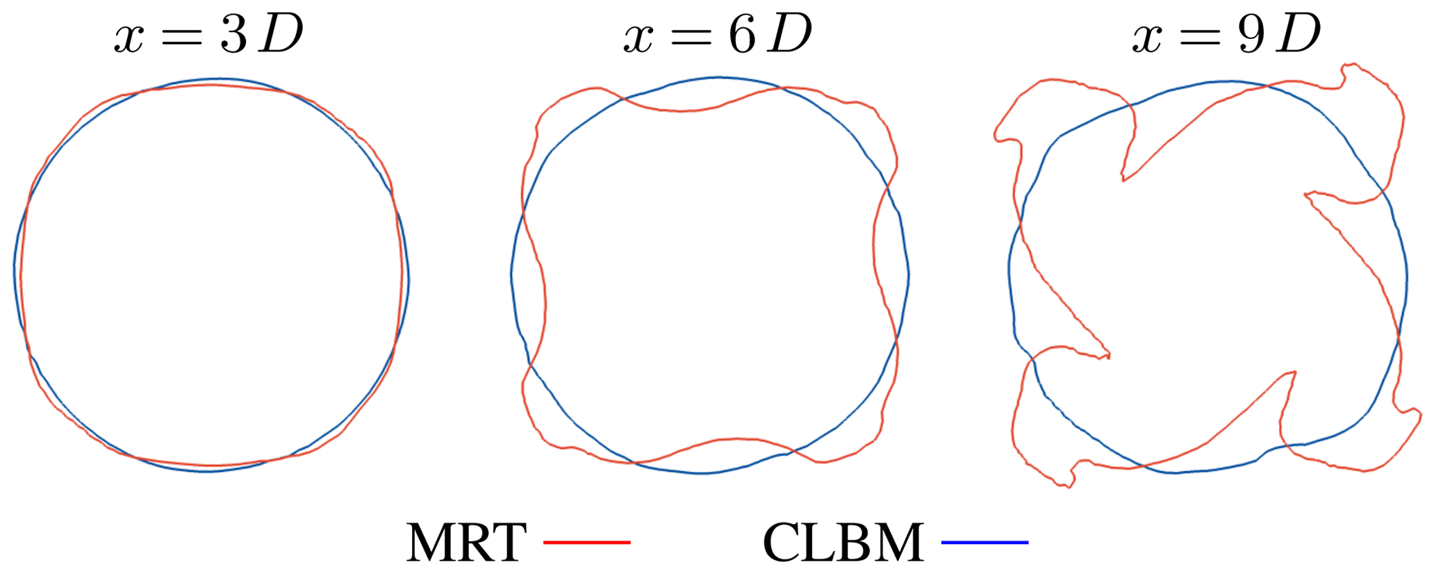
Figure A1 Instantaneous velocity contours (u=0.875 u₀) in cross-sectional planes at different positions in the wake of the turbine.