Validation and accommodation of vortex wake codes for wind turbine design load calculations

The computational effort for wind turbine design load calculations is more extreme than it is for other applications (e.g., aerospace), which necessitates the use of efficient but low-fidelity models. Traditionally the blade element momentum (BEM) method is used to resolve the rotor aerodynamic loads for this purpose, as this method is fast and robust. With the current trend of increasing rotor size, and consequently large and flexible blades, a need has risen for a more accurate prediction of rotor aerodynamics. Previous work has demonstrated large improvement potential in terms of fatigue load predictions using vortex wake models together with a manageable penalty in computational effort.

The present publication has contributed towards making vortex wake models ready for application to certification load calculations. The observed reduction in flapwise blade root moment fatigue loading using vortex wake models instead of the blade element momentum (BEM) method from previous publications has been verified using computational fluid dynamics (CFD) simulations. A validation effort against a long-term field measurement campaign featuring 2.5 MW turbines has also confirmed the improved prediction of unsteady load characteristics by vortex wake models against BEM-based models in terms of fatigue loading. New light has been shed on the cause for the observed differences and several model improvements have been developed, both to reduce the computational effort of vortex wake simulations and to make BEM models more accurate. Scoping analyses for an entire fatigue load set have revealed the overall fatigue reduction may be up to 5 % for the AVATAR 10 MW rotor using a vortex wake rather than a BEM-based code.

1 Introduction

For wind turbine design certification, load calculations in agreement with IEC guidelines (International Electrotechnical Commission, 2019) are required to define a representative load envelope. Because wind turbines operate in the atmospheric boundary layer, they are subject to a large variety of inflow conditions in terms of spatial and temporal variation in wind speed and direction due to the occurrence of gusts, shear and turbulence. To cover this wide range and determine representative fatigue and extreme loads, a large number of load cases need to be simulated in the time domain using aeroelastic codes. These codes generally include models for the structural dynamics of tower, drivetrain and blades; a model for the rotor speed and pitch controller; and aerodynamic models for rotor and tower. This implies a large number of rotor aerodynamic iterations are needed as well, which necessitates the use of efficient but low-fidelity models (Schepers, 2012). Hence for a reliable wind turbine design, dependable aerodynamic models are needed. However the uncertainty margins associated with these models are large, which especially holds true for the unsteady rotor aerodynamics (Boorsma and Schepers, 2018). The current trend of increasing rotor size, and consequently large and flexible blades, has together with the larger inflow variations over the rotor disk resulted in a greater relative importance of unsteady flow features and the modeling thereof. This further underlines the need for more accurate prediction of rotor aerodynamics. At this moment roughly three categories of aerodynamic models are available:

1. blade element momentum (BEM) models,

2. vortex wake models, and

3. computational fluid dynamics (CFD) models.

In the industry, the BEM method is the workhorse for wind turbine certification load calculations. The development of more advanced codes like vortex wake models for wind turbine applications started in early 2000 (Belessis et al., 2001; van Garrel, 2003). Vortex wake models give a more accurate description of the rotor wake aerodynamics but are more computationally expensive because they actually resolve the wake geometry instead of only the rotor plane. Nevertheless with increasing computational power, vortex wake models are posing a good alternative to BEM. The vortex wake models in this research are all low-order vortex filament methods. As part of the EU project AVATAR (Schepers, 2016) a fatigue load comparison round was performed between various aeroelastic codes using BEM and vortex wake models. Calculations were done featuring the AVATAR 10 MW rotor in turbulent inflow for a variety of time-averaged wind speeds. Two partners independently of each other showed a reduction of roughly 15 % of the blade out-of-plane fatigue equivalent moments when switching from a BEM to a vortex-wake-type model for the evaluation of rotor aerodynamics (keeping the other parameters such as the structural dynamic model the same). In addition large differences were found in the implementation of the BEM models. More results are given in the dedicated AVATAR report (Boorsma et al., 2016a). Over the last decades several publications have researched the added benefit of vortex wake models over BEM-based models (Hauptmann et al, 2014; Gupta, 2006; Boorsma et al., 2016b) and more recently (Perez-Becker et al., 2019). Some of these feature a validation against wind tunnel data, for which the inflow conditions and turbine are not always representative for design load calculations on a multi-megawatt wind turbine. Others, such as the mentioned AVATAR report, feature a comparison between BEM and vortex wake models for more representative conditions, but they lack a validation since experimental data for these conditions are not available. Although one would expect a higher-fidelity model to be more accurate, validation and verification of the outcome are required to confirm the measured load prediction reduction from vortex-wake-type codes.

Within this mindset the TKI WoZ VortexLoads project (Boorsma et al., 2019c) was started in which ECN.TNO, DNV-GL, LM Wind Power and GE have cooperated towards evaluating and accommodating the application of vortex wake models to certification load calculations. A comparison against dedicated CFD simulations in turbulent inflow conditions is carried out and described in Sect. 2. A validation against a large field measurement database, which comprises long-term measurements to reduce the uncertainty in inflow conditions between measurements and simulations, is given in Sect. 3. Lastly Sect. 4 describes the impact of running a production load set with a vortex wake rather than a BEM-type code.

2 Verification against CFD simulations

CFD simulations are carried out to verify the differences in dynamic loading and the resultant fatigue equivalents between BEM and vortex wake codes. The AVATAR 10 MW wind turbine model that originated from the AVATAR project (Schepers, 2016) was the subject of this study. With a rotor diameter of 205.8 m this turbine features a relatively low power density of around 300 W m⁻², operating at a design axial-induction factor of around 0.2. To be able to compare to CFD, a rigid (or non-flexible) version of the turbine was used. The various codes used in the comparison round and their settings are described first below. The initial focus is on comparisons in uniform, constant inflow and vertically sheared inflow, after which several cases with turbulent inflow conditions are studied.

2.1 Code descriptions

2.1.1 FLOWer

A CFD reference solution using the AVATAR 10 MW rotor was calculated with the process chain for simulations of wind turbines developed at the Institute of Aerodynamics and Gas Dynamics (IAG, USTUTT) in the last years (i.e., Schulz et al., 2016). The main part of the chain is the CFD code FLOWer, which is complemented by different preprocessing and post-processing tools. The CFD code FLOWer was developed by the German Aerospace Center (DLR) within the MEGAFLOW project (Kroll et al., 2000) in the late 1990s. It is a compressible code and solves the three-dimensional Navier–Stokes equations in an integral form with several turbulence models. The numerical scheme is based on a finite-volume formulation for block-structured grids. For the spatial discretization, a second-order central discretization with artificial damping, the Jameson–Schmidt–Turkel (JST) (Jameson et al., 1981) method, and the fifth-order weighted essentially non-oscillatory scheme WENO (Jiang and Shu, 1996) are available. Time integration is accomplished by an explicit multistage scheme. Time-accurate simulations use the dual-time-stepping method as an implicit scheme. The pseudo time iterations can be accelerated with the same methods as steady computations.

To close the Navier–Stokes equation several Reynolds-averaged Navier–Stokes (RANS) and hybrid RANS–large-eddy simulation (LES) turbulence models were implemented in FLOWer. The turbulence model equations are solved separately from the main flow equations using a full implicit time integration method. The ROT module allows body motions in translating/rotating reference frames for unsteady wind turbine simulations. FLOWer is optimized for parallel computing and uses the Message-Passing Interface (MPI). A no-slip wall condition was used on the blade surface without any wall function, and a far-field condition was applied in the cross-flow directions. For the current task the IDDES model (Shur et al., 2008) based on Menter shear stress transport (SST) k−ω (Menter, 1994) was adopted, and no transition model was considered; i.e., fully turbulent simulations were conducted. A second-order dual-time-stepping method was adopted for the time discretization, and a five-stage Runge–Kutta scheme was used for every inner iteration. The JST scheme was adopted for the blade meshes, and the fifth-order WENO scheme was adopted for the background mesh.

Block-structured meshes were generated separately for the blade and background, and they were combined without sacrificing the quality of the meshes by using the Chimera overlapping grid technique (Chesshire and Henshaw, 1990). A blade mesh convergence test was performed in a previous study (Bangga et al., 2017). The blade mesh is a C-type mesh with 280 grid cells × 128 grid cells × 192 grid cells in the chord, wall-normal and span-wise directions. The first wall-off cell size is less than $\mathrm{3}\times {\mathrm{10}}^{-\mathrm{6}}$ m, which satisfies the condition $y_{\mathrm{1}}^{+}<\mathrm{1}$. The domain size was set to 3584 m × 1792 m × 1792 m in the stream-wise (x) and two cross-flow (y, z) directions. The rotating axis was aligned with the x axis and located at the origin, which was at a distance of 1536 m from the inlet boundary. The total number of cells for simulations with the rotor was 123.5×10⁶.

For the turbulent inflow cases, the wind fields were generated using the Mann turbulence generator from DTU Wind Energy. The generated turbulence field was injected at $x=-\mathrm{400}$ m using a momentum source term (Troldborg et al., 2014),

$$f_{E_i}={\displaystyle \frac{\mathit{\rho }{u}_i^{\prime }}{\mathrm{\Delta }{x}_n}}\left(U_n+{\displaystyle \frac{\mathrm{1}}{\mathrm{2}}}{u}_n^{\prime }\right),$$

where the subscript “n” indicates the normal component to the turbulence plane. It is noted that the Gaussian convolution, which was used in Troldborg et al. (2014) to avoid numerical oscillation, was not applied because such oscillations were not observed with the numerical scheme used near the turbulent plane, i.e., fifth-order WENO. The time step was set to be approximately 1^∘ azimuthal variation in the blades per time step. To account for controller-initiated changes in rotation speed and pitch, the variations in rotation speed and pitch were recorded during BEM simulations with controller (featuring the same turbulent wind field) and prescribed to the CFD simulation via approximated Fourier series. More detail about the set-up of the CFD simulations can be found in Wenz et al. (2019) and Boorsma et al. (2019b).

For a better agreement between lifting-line and CFD simulations, the airfoil data for the lifting-line simulations were determined from 3-D CFD simulations (Bangga et al., 2017; Bangga, 2018). To vary the angle of attack seen by the blade sections, the inflow wind speed is artificially increased or decreased by maintaining the rotational speed constant at 9.02 rpm. The effective angle of attack seen by the blade sections is then calculated using the reduced axial velocity method, often denoted as the azimuthal averaging technique, according to Hansen et al. (1997). The method takes the averaged velocity upstream and downstream of the rotor plane and linearly interpolates the relative velocity at the rotor plane. The resulting polars include the rotational augmentation effects; hence modeling of these should be disabled in the lifting-line simulations. Also, the Prandtl effect due to the finite number of blades is implicitly included in the CFD simulations. Therefore the polars for the outboard sections (>70 % R) are determined from 2-D CFD simulations, as this effect cannot be switched off for the vortex wake simulations. Although the resulting angle-of-attack range covered the operational regime well for the cases under consideration, it was extended beyond that using the original polar dataset of the AVATAR turbine.

2.1.2 Bladed 4.8

The results provided by DNV-GL are based on the BEM code of Bladed 4.8. The BEM code in Bladed 4.8 is completely rewritten and replaces the code used in Bladed 4.7 and lower. Recent public validation work is presented in the references Collier and Sanz (2016) and Schepers and Boorsma (2014). The model is based on classical BEM theory where the axial and tangential Glauert momentum equations are expressed in dimensional form instead of nondimensional factors. Further, the dynamic submodels (dynamic wake, dynamic stall, skew wake correction) are fully expressed in state-space form, allowing combined direct integration of structural and aerodynamic states. The aerodynamic and structural states are integrated with a fourth-order variable-step Runge–Kutta integrator. The engineering correction models used in the Bladed 4.8 BEM code are the Øye and Pitt and Peters dynamic wake model (described in Snel and Schepers, 1994), Beddoes–Leishman dynamic stall model in state-space format, Glauert skew wake correction method, Prandtl tip correction, and Glauert corrections for highly loaded rotors.

Next to the classical BEM model, Bladed 4.8 and higher feature a fully coupled free-wake lifting-line model. At present this code is used for internal purposes only and is not yet commercially released. The theory of the lifting-line code is described in Kloosterman (2009). Recent work published with the code is found in Schepers and Boorsma (2014) and Harrison et al. (2018). The implementation in Bladed is however fully coupled to the Bladed multibody model and allows for aeroelastic load simulations. For the turbulent inflow test cases, a time step which is approximately equivalent to one step per degree of revolution was applied. Special effort has been made to ensure efficient parallelization and vectorization of the code. It is also possible to distinguish between wake update frequency and aerodynamic time step, which has great potential for reduction of computational time (Boorsma et al., 2019a).

2.1.3 ECN Aero-Module

The ECN (Boorsma et al., 2011, 2016b) includes two aerodynamic models, the BEM method similar to the implementation in Phatas (Lindenburg and Schepers, 2000) and a free-vortex wake code in the form of an aerodynamic wind turbine simulation model (AWSM) (van Garrel, 2003). Both models are lifting-line codes; i.e., they make use of aerodynamic look-up tables to evaluate airfoil performance. The set-up allows us to easily switch between the two aerodynamic models whilst keeping the external input the same, which is a prerequisite for a good comparison between them. Although the package can be coupled to simulation software that solves the structural dynamics of a wind turbine (FOCUS, LM Wind Power, 2016; SIMPACK, DS Dassault Systems, 2018), the stand-alone option is used to simulate a rigid turbine with prescribed operational conditions. The BEM model features a local implementation, i.e., solving the momentum equations separately for each blade element rather than once for a full annulus. Several engineering extensions are used such as a dynamic inflow model (Snel and Schepers, 1994), yaw model (Schepers and Vermeer, 1998; Schepers, 1999), root and tip loss model (Prandtl and Betz, 1927), and a turbulent wake state model (replacement of the theoretical momentum equation with a linear relation between thrust coefficient and axial-induction factor above a value of 0.38 for this parameter).

The Snel first-order dynamic stall model (Snel, 1997) was applied to all simulations (unless explicitly stated otherwise), and rotational corrections were disabled. For the free-vortex wake simulation, the number of wake points was chosen to make sure that the wake length was developed over at least three rotor diameters downstream of the rotor plane. The wake convection was free for the first two wake diameters downstream of the rotor plane. For the remaining wake length, the averaged induction (for each blade vortex sheet) at the free-to-fixed wake transition is applied to all wake points. For both aerodynamic solvers approximately 20 elements in the spanwise direction were used. The spanwise discretization in AWSM approximates a cosine distribution, whereas this is linear for BEM, featuring half the spacing at the tip. For the turbulent inflow calculations, the time step was kept at the approximate equivalent of 1^∘ azimuth for both the BEM and AWSM simulations. Wake reduction (Boorsma et al., 2018) (reducing the shed vorticity spacing) was applied after approximately half a diameter convected wake, skipping nine shed vortices to end up with an effective distance of 10^∘ azimuth between the shed vortices in the remaining part of the wake. This typically results in about 500 streamwise wake points and hence about $\mathrm{500}\times \mathrm{20}\times \mathrm{3}=\mathrm{30}\mathrm{000}$ vortex filaments for a simulation.

2.1.4 Phatas

The computer program Phatas, “Program for Horizontal Axis wind Turbine Analysis and Simulation” (Lindenburg and Schepers, 2000), is developed for the time-domain calculation of the dynamic response and the corresponding loads on a horizontal axis wind turbine. The program Phatas is available as tool in the integrated wind turbine design package FOCUS6 (LM Wind Power, 2016). The program Phatas has its own “internal” BEM-based aerodynamic model but is also available in a configuration PhatAero that uses the aerodynamics from the coupled ECN Aero-Module.

The internal BEM-based aerodynamic model features several engineering extensions such as a dynamic inflow model (Snel and Schepers, 1994), yaw model (Schepers and Vermeer, 1998; Schepers, 1999), root and tip loss model (Prandtl and Betz, 1927), and turbulent wake state model based on the formulation of Wilson. For the airfoil data, the modeling of dynamic stall behavior (Snel, 1997) and rotational effects on lift (Snel et al., 1993) is optional based on Snel's models. The internal model features a recent addition to account for the effects of shed vorticity (blade shed vorticity), which calculates a vortex structure of shed vorticities based on the time history of the lift coefficients and the relative velocities of the airfoils (Boorsma et al., 2019a).

The blades were modeled with 31 elements over the span, where 29 elements have equal length and the two elements close to the tip have half that length. The aerodynamic stagnation from the tower was not included. The time increment was set to give a 1^∘ increment in rotor azimuth.

The input settings of PhatAero + ECN Aero-Module AWSM are for a six-diameter total wake length of which two diameters are for a free-geometry wake length. The calculations were done with the option to skip the “odd” aero calls, which reduces the number of aerodynamic evaluations and likewise reduces the CPU needed. The simulations featuring the blade shed vorticity model (indicated by Phatas-BSV) incorporate the effect of 20 shed vortices. A high-level overview of the codes used is given in Table 1.

Table 1 High-level overview of codes and settings.

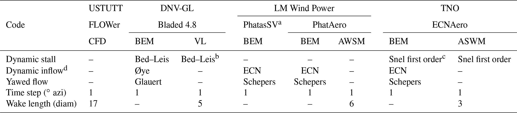
^a PhatasSV-BSV is also used which contains a separate shed vorticity model. ^b Shed vorticity effects excluded for vortex wake simulations. ^c Beddoes–Leishman model was used for several cases (ECNAero-BEM-BL). ^d See text for implementation differences.

Table 2 Summary of uniform and sheared inflow comparison cases.

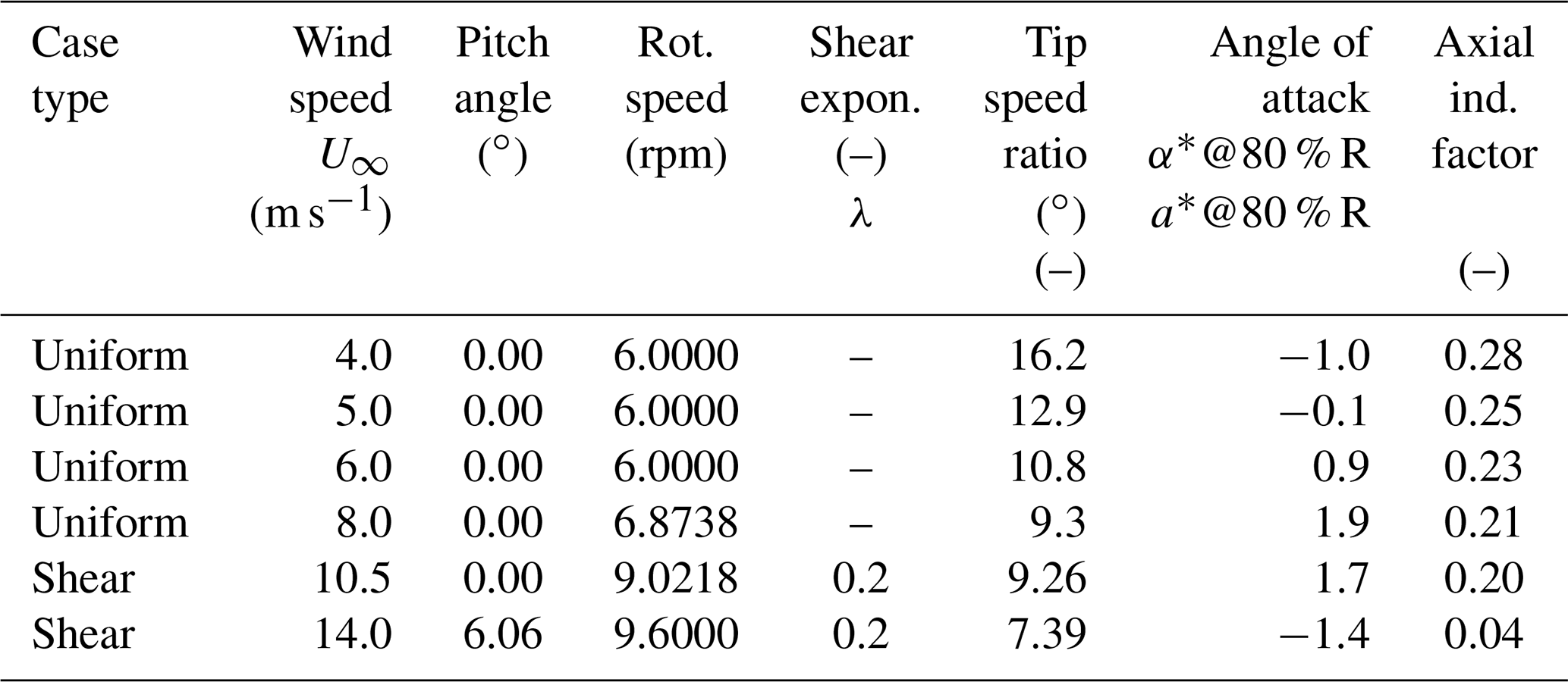
^* Estimate.

Figure 1 Load comparison in uniform inflow conditions.

Figure 2 Azimuthal variation and amplitudes in shear, U_∞=10.5 m s⁻¹.

2.2 Constant uniform and sheared inflow

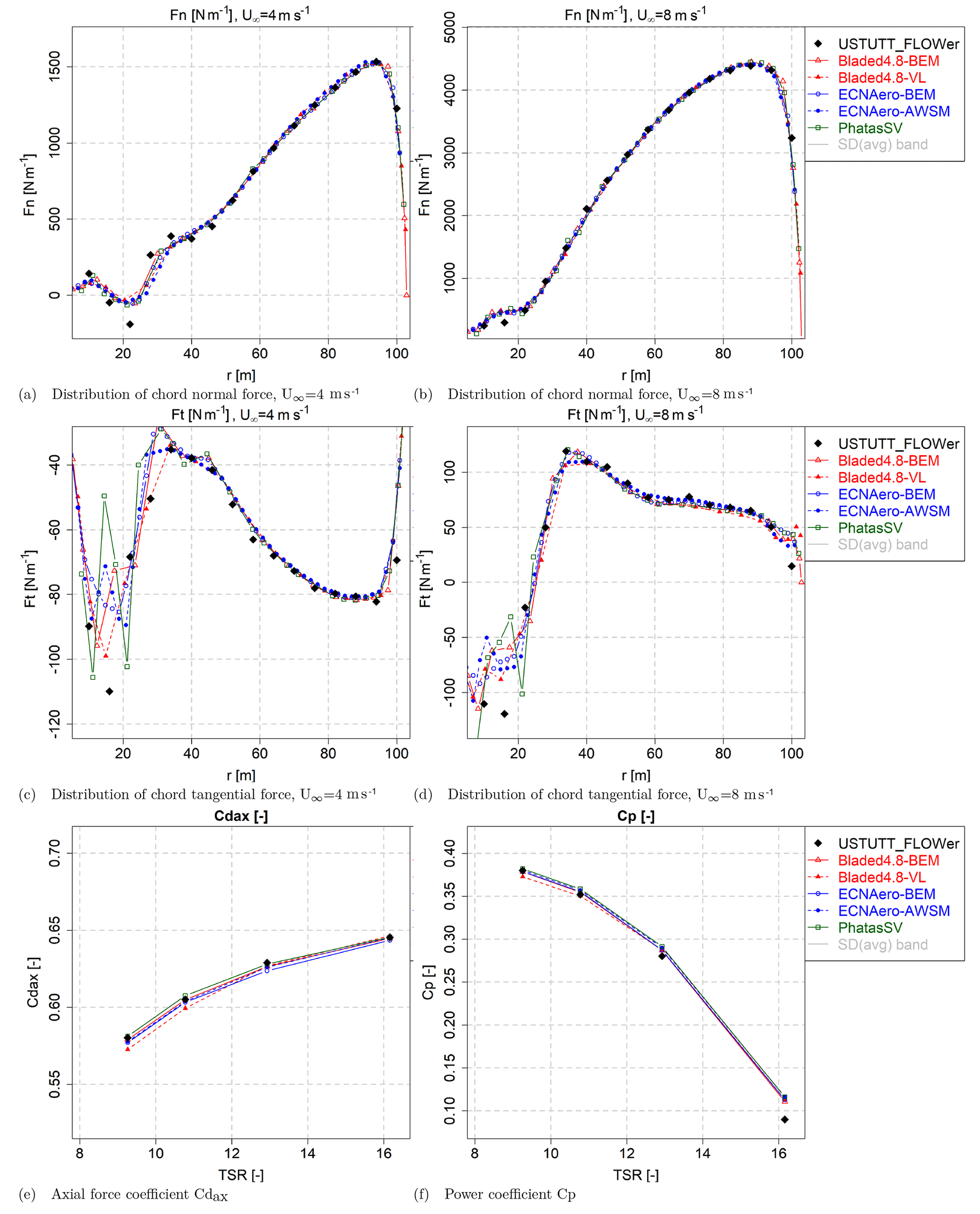
Four uniform inflow cases were simulated following part of the power curve, as summarized in Table 2. The resulting load comparison is given in Fig. 1 for the radial distribution of chord normal and tangential force, plus the deduced integral aerodynamic variables axial force and power. It is observed that generally speaking a good agreement is found between lifting-line and CFD simulations, which is attributed to the polars being generated from 3-D CFD simulations as described in Sect. 2.1.1. The good agreement is a prerequisite for a successful comparison of unsteady aerodynamics in sheared and turbulent inflow conditions.

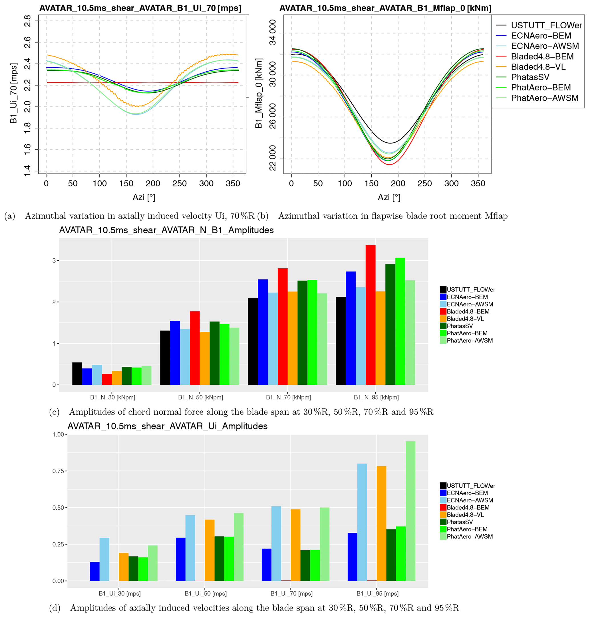
In addition two vertically sheared inflow cases were simulated (see also Table 2). Looking at the flapwise blade root moment variation in Fig. 2a, we can observe differences between the predicted amplitudes of the codes. These differences grow larger for the underlying axially induced velocities in Fig. 2b. Here it is noted that “lifting-line variables” such as angle of attack and induced velocities are not available for the CFD results and hence are not displayed.

To better observe the differences, the simulation results are post-processed to average values and amplitudes (by evaluating the difference between maximum and minimum values) of the fluctuation along a rotor revolution. The remaining plots of Fig. 2 show the results of the amplitude comparison, and here we do observe a striking difference between vortex wake and BEM-type codes. The BEM-type codes systematically overpredict the amplitudes of the normal forces in comparison to the CFD and vortex wake results (that are in relatively good agreement), consistent along the blade span except for the most inboard station at 30 % R. The difference can be traced back to the angle of attack and the underlying axially induced velocity variation in Fig. 2d, which can be considered the “heart” of lifting-line models. For the vortex wake codes, the axially induced velocity follows the inflow velocity variations more extremely as the blades rotate through the sheared velocity field. Between the BEM codes it can also be observed that whereas some of them predict a substantial azimuthal variation in axially induced velocity, there are also BEM results where this azimuthal variation along a rotor revolution is almost negligible. It is known that a wide variety of BEM implementations exist, e.g., solving the momentum equations for a whole annulus or per element, not to mention the interaction with a dynamic wake or dynamic inflow model. This example illustrates the effect these implementation differences can have. Application of the dynamic inflow model to the local-element-induced velocity (as implemented in the Bladed 4.8 BEM results following the TUDK model as described in Snel and Schepers, 1994) appears to dampen out induced velocity variations in nonuniform inflow conditions. The other BEM codes use a similar dynamic inflow model, but the dynamic inflow term is related to the annulus-averaged induced velocity rather than its respective element value, which results in better tracking of inflow variations.

In search of a fundamental reason for the difference between BEM and vortex wake codes, calculations were done for various conditions (ranging between 6 and 18 m s⁻¹ wind speed) with the PhatasSV and PhatAero code. These calculations also included two-bladed and four-bladed versions of the AVATAR rotor. For the two-bladed rotor models the chord distribution is simply 1.5 times larger compared to the chord distribution of the three-bladed rotor. The four-bladed rotor model has 75 % of the chord distribution compared to the three-bladed rotor. This “scaling” gives a similar rotor disk loading except near the blade tip. For all configurations the solidity of the rotor is 0.0408. The result shows that for all operational conditions the 1P variation in the blade root flap moment from the BEM-based calculations is larger than from the AWSM calculations. This seems to be related to the axial-induction factor; see also Fig. 3. Although the values of the axial-induction factor are not distributed homogeneously, a nearly quadratic trend follows for the ratio between blade root flapwise bending moment variation from BEM simulations compared to the vortex wake (AWSM) simulations. The ratio between root moment variations shows to be quite insensitive to the number of rotor blades or the distance between the vortex sheets of the blades.

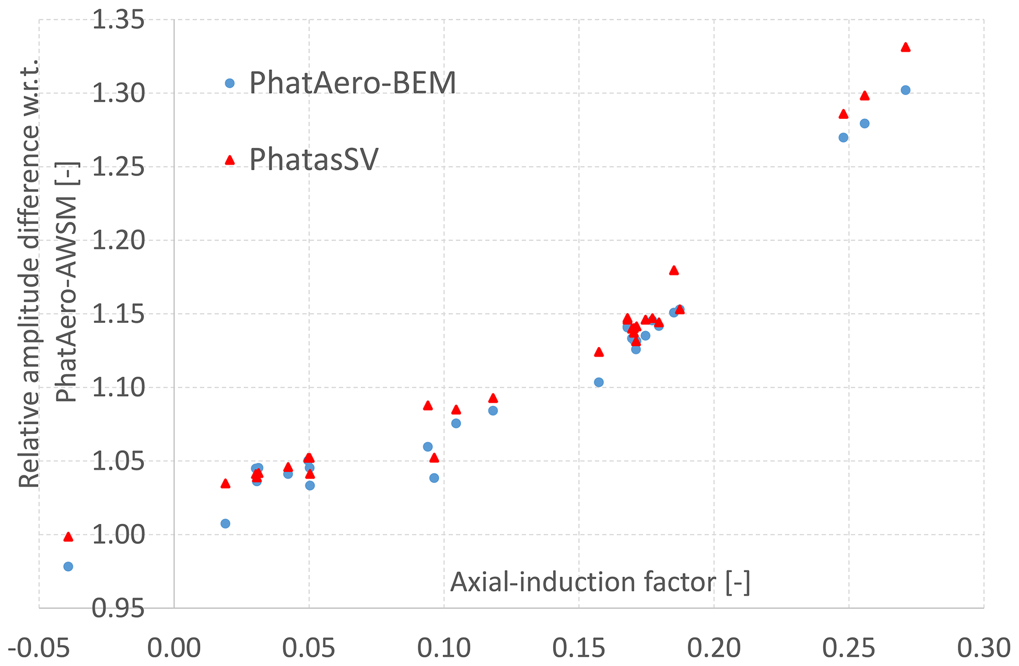
Figure 3 Relative difference of Mflap amplitudes from BEM calculations in shear with respect to PhatAero-AWSM versus axial-induction factor.

Table 3 Turbulent inflow comparison cases.

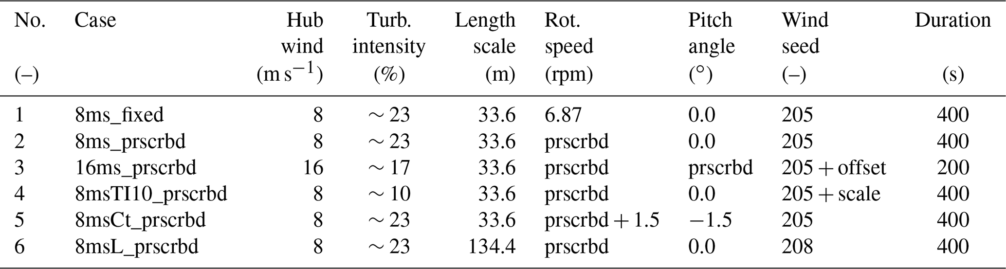
2.3 Turbulent inflow

After exposing the differences between the codes in sheared inflow, the next step is a comparison in turbulent inflow. Six cases were simulated, as summarized in Table 3. To ensure all partners read the turbulent wind file in the same way and signal processing is in agreement amongst the partners, first an alignment study was performed using a 150 s simulation from the EU AVATAR project (Kim et al., 2016), which featured a constant pitch and rotational speed at an average hub height wind speed of 10.5 m s⁻¹. The cases summarized in Table 3 are defined in agreement with IEC Class 1A, although wind shear was excluded from the comparison. The first case featured a constant rotational speed and pitch angle at 8 m s⁻¹ hub height wind speed. For the AVATAR turbine the class 1A specification leads to a rather high turbulence intensity of 23 % and a length scale of 33.6 m. Seed selection was determined by running six different seeds with BEM and matching the most representative seed to the average values of fatigue, mean and standard deviation over the six seeds. Wind field duration was set to 400 s (16 m s⁻¹ case excepted) based on a compromise between computational expense and a good statistical representation. For the second case, a BEM simulation with the AVATAR controller activated was performed with the wind seed under investigation. The resulting rotational speed and pitch angle variations were recorded and fed to CFD, BEM and vortex wake simulations (this is indicated by the suffix “prscrbd”). The same procedure was adopted for the other cases. Since the wind speed was below rated, the resulting pitch angle remained constant for this case at 0^∘. For the third case the same wind seed was used but the offset was increased to result in an average of 16 m s⁻¹ hub height wind speed. Acknowledging that a wind seed turbulence box has a constant length, doubling the wind speed effectively means that the simulation duration is halved to 200 s. In agreement with IEC Class 1A specifications, the wind speed fluctuations were scaled to match an average turbulence intensity of roughly 17 %. For the fourth case, the influence of varying the turbulence intensity was investigated by scaling the amplitude of fluctuations for the same seed to approximately 10 %. For the fifth case, the influence of an increased thrust coefficient or axial-induction factor was investigated. With this aim an offset was applied to the rotational speed and pitch angle variation in the second case. This way the operating angle of attack was not significantly different from the second case, and the spanwise variation in the averaged axial induction remained relatively constant. Finally for case six, the influence of a different length scale was investigated by increasing this parameter with a factor of 4. The idea behind this case is to mimic the effect of rotor size by changing the turbulence length scale. It is anticipated that the rotational sampling will be different between small and larger rotors, influencing the coherence of the encountered wind gusts. For more info on the case description, please consult the dedicated report from the University of Stuttgart (Wenz et al., 2019) on this subject.

2.3.1 Comparison methodology

In cases with turbulent inflow, besides a statistical evaluation, analyzing the development of forces over time is an interesting approach which might give more insight. In order to do this, a consistent input of background turbulence in the different codes has to be ensured. In CFD, turbulence is altered as it propagates through the domain until it reaches the rotor, while in BEM and vortex wake models, the flow field, i.e., turbulence, is applied directly to the rotor. Moreover, the propagation in CFD is slowed down in front of the turbine due to the rotor blockage. To allow a time-dependent load comparison between the codes, these CFD effects need to be compensated for in the lifting-line code input. This was achieved by extracting the turbulent velocity field from the empty box CFD simulations and applying a time shift to compensate for the blockage effect. A detailed explanation of the method is given elsewhere (Wenz et al., 2020, 2019)

The resulting alignment between the codes was verified by comparing the values of the encountered wind by the blades using virtual “wind probes” at several radial stations. Generally speaking a good agreement of the encountered wind variation as a function of time was found using this method, indicating that the turbulence structures from empty box and rotor CFD are highly alike, providing similar fluctuations due to the rotational sampling. However it should be realized that although this method comes close, definition of identical inflow conditions between CFD and lifting-line codes is impossible and the current approach is an approximation based on an engineering method. As such, small inflow differences between lifting-line codes and CFD remain.

Figure 4 Key results for the U_∞=8 m s⁻¹ fixed rotational speed and pitch angle case (first case from Table 3).

2.3.2 Differences between the models

To study the differences between the codes, the statistics (minimum, maximum, average, standard deviation) over the full time series were determined as well as the 1 Hz equivalent loading (based on the rain flow counting procedure using a slope of m=11) for a large number of variables. Despite the small differences in inflow definition, the 8 m s⁻¹ fixed case (i.e., fixed rotational speed and pitch angle) allows us to draw some interesting conclusions with respect to the effects of modeling differences. A summary of key results from this case is shown in Fig. 4. In agreement with results from the AVATAR project and the sheared inflow comparison, the induced velocity variation in vortex wake models follows the underlying inflow variations more directly than the BEM results. The vortex wake model from Bladed features the same behavior as the previously studied vortex wake models. As a result, the fluctuations in angle of attack and consequently aerodynamic loads are smaller (within the sectional velocity triangle the change in wind speed is partly compensated for by the change in axial induction). This is clearly affecting the equivalent sectional load levels at all radial stations (inboard at 30 % R often excepted) and hence also the blade root moments. The comparison to CFD indicates that generally speaking the vortex wake codes agree better with CFD than BEM judging by the magnitude of load fluctuations and resulting equivalent load levels.

From previous work (Boorsma et al., 2016a) it was hypothesized that part of the observed difference between BEM and vortex wake codes can be explained by the shed vorticity modeling which is implicitly included for vortex wake models but not in BEM. A dedicated model to simulate the effect of shed vorticity changes has been developed for the PhatasSV code, called Phatas-BSV; see also Sect. 2.1.4. It is also noted that the indicial method from Beddoes and Leishman (Leishman and Beddoes, 1986, 1989) for modeling unsteady sectional aerodynamics includes a part dedicated to modeling shed vorticity effects based on Theodorsen's theory (Theodorsen, 1935). As an alternative to Snel's dynamic stall model, this submodel was applied in the ECN Aero-Module (ECNAero-BEM-BL). The resulting fatigue equivalent blade root moments displayed in Fig. 5 indeed confirm that modeling shed vorticity partly reduces the discrepancy between BEM and vortex wake codes. In addition to that it is observed that both the blade shed vorticity model in PhatasSV (which acts on the induced velocities by modeling a shed vorticity structure) and the Theodorsen part of the Beddoes–Leishman model (which acts on the airfoil coefficients rather than induced velocities) result in a similar effect on the fatigue equivalent moments.

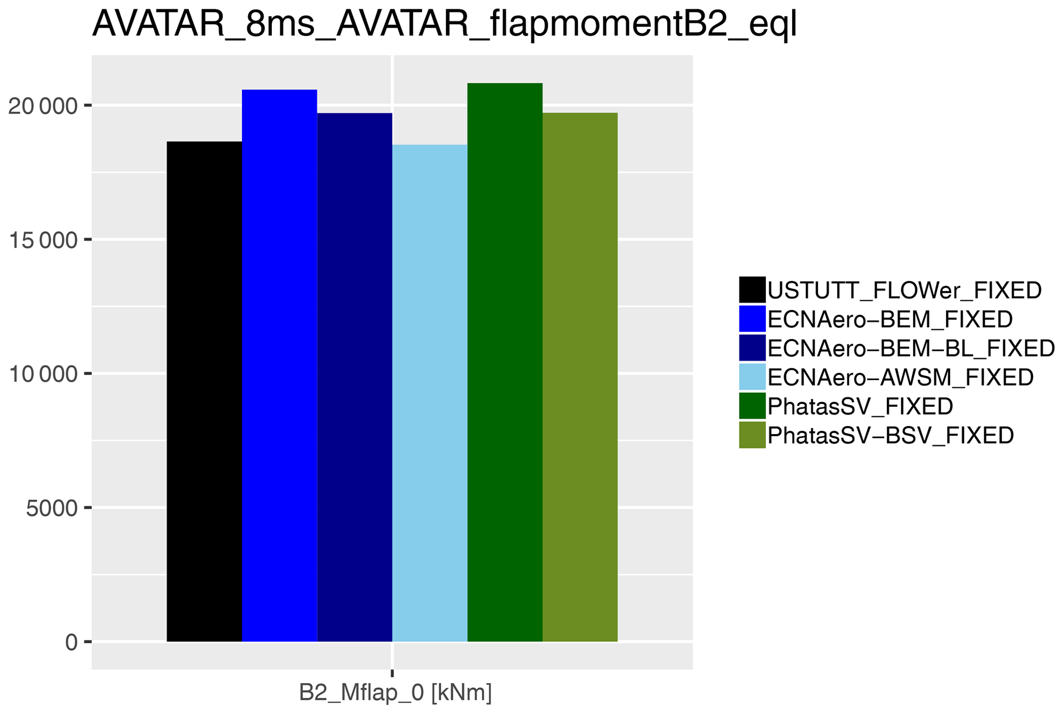
Figure 5 Effect of shed vorticity modeling on fatigue equivalent flapwise blade root moment for the first case from Table 3 (fixed rotational speed). The legend addition “BSV” stands for the blade shed vorticity model in PhatasSV, while “BL” indicates usage of the Beddoes–Leishman model instead of the Snel model for unsteady airfoil aerodynamics.

Studying the axially induced velocity variations in Fig. 4a reveals large differences not only between BEM and vortex-wake-type codes, but also between the different BEM codes. Where the red line shows a nearly constant level, the other BEM codes feature more variation with inflow velocity. This was also observed in the sheared inflow comparison as described in Sect. 2.2. Here this difference was found to be related to the various implementations of the dynamic wake or dynamic inflow model, which can result in dampening of induced velocity variations due to inflow fluctuations.

2.3.3 Effect of load case variations

For several cases the earlier mentioned small differences in inflow conditions between CFD and lifting-line codes influence the equivalent load levels, as the result of the rain flow counting is dominated by the largest fluctuation over the time series. Therefore it is decided to study the staircase plots from the rain flow counting procedure, which are an intermediate result showing the range of fluctuations versus the number of occurrences or counts. Instead of focusing on the equivalent load level determined by the largest ranges with very few occurrences, statistically it makes more sense to study the ranges with a large number of counts when comparing CFD to lifting-line simulations. To compare the results between the codes over the simulated load cases, the staircase plots of the flapwise blade root moments (e.g., Fig. 4c) were integrated (starting at a threshold of 10 counts, keeping the logarithmic distribution for the number of counts). A summary of the results is given in Fig. 6.

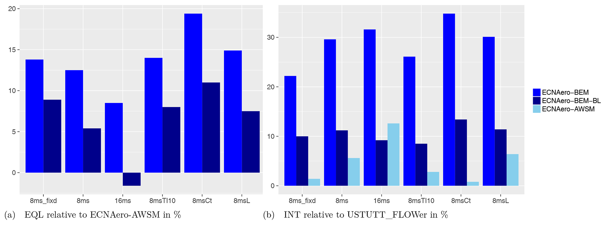
Figure 6 Relative difference of fatigue equivalents (EQL) and integrated staircase plot values (INT) of flapwise blade root moments for the turbulent inflow cases. Values are averaged over three blades, and staircase plots are integrated from a threshold value of 10 counts.

In agreement with the results of the 8 m s⁻¹ fixed case, the vortex wake results tend to agree well with CFD for the other cases also. Drawing a general conclusion on variations between the load cases is complicated because observed differences between the cases can potentially be caused by the difference in specific turbulence boxes (seeds) and the way the rotor blades slice through them. It seems that similar to the shear case, a higher thrust coefficient value results in larger differences between BEM on the one hand and vortex wake and CFD models on the other hand. The 16 m s⁻¹ result features a very low thrust (axial-induction factor around 0.06), which makes the BEM with shed vorticity modeling come very close to the vortex wake model, although a rather high unexplained difference remains with CFD. Simulating a higher length scale (mimicking a 4-times-smaller turbine) unexpectedly seems to have hardly any impact on the magnitude of the differences between the models.

Although comparison of equivalent loads between CFD and lifting-line codes is hindered by small differences in inflow conditions, a comparison between lifting-line codes (BEM and vortex wake) in terms of fatigue loading is deemed useful in Fig. 6b. These numbers also confirm that the shed vorticity modeling in BEM for this 16 m s⁻¹ case makes these results come very close to the vortex wake results, and this difference to be at a maximum for the high thrust case. It can also be observed that, although the absolute level of the flapwise fatigue load will decrease with a lower turbulence intensity, the relative difference between BEM and vortex wake code results remains similar. For more details the full report (Boorsma et al., 2019b) about the comparison between lifting-line and CFD simulations can be consulted.

2.4 Improved induction tracking

From Sect. 2.2 it appears that a difference exists between the predicted load fluctuation amplitudes in vertical shear from vortex wake (AWSM) and BEM-type codes, which correlates with the axial-induction factor. Application of an engineering extension to BEM, accounting for the effect of shed vorticity variation, did not yield an explanation for this difference. Most likely the gradual inflow variations in vertical shear are not abrupt enough for the shed vorticity variation to play an important role. In turbulent inflow (see also Fig. 5), shed vorticity and dynamic inflow can explain part of the observed differences between BEM and vortex wake modeling. In an attempt to further study the cause for the remaining difference, results from BEM and vortex wake sheared inflow simulations on the AVATAR rotor have been post-processed to verify compliance with the axial momentum equations. The one-dimensional axial momentum equations constitute a relation between the thrust coefficient C_t and the axial-induction factor a at the rotor disk in the form of

$$\begin{array}{}\text{(1)}& C_{\mathrm{t}}=\mathrm{4}a(\mathrm{1}-a)\mathrm{and}a=U_{\mathrm{i}}/U,\end{array}$$

with C_t (–) the thrust coefficient, a (–) the axial-induction factor at the rotor disk, U_i (m s⁻¹) the axially induced velocity and U (m s⁻¹) the wind speed.

It is noted that C_t is based on the force of a single blade element and a the axial induction for the corresponding annulus, hence corrected for the finite number of blades using the Prandtl tip loss factor (BEM) or by averaging the induced velocities over the annulus (AWSM). To be able to focus on the effect of shear, a relatively large shear exponent of 0.75 at 8 m s⁻¹ hub height wind speed was employed for the investigation. The results in Fig. 7a indicate that the BEM simulation complies with the underlying momentum equation as it is supposed to. However the vortex wake results in Fig. 7b clearly deviate from this line depending on the azimuthal position, where especially for the outboard stations high thrust coefficients are obtained in combination with a relatively low axial-induction factor (lower as would be the case for the theoretical momentum line) for a downward-pointing blade featuring the lowest local inflow velocity. It can be shown that for rotors operating at higher induction, BEM theory can even predict an increase rather than decrease in axially induced velocity when the blade is pointing downward (6 o'clock position), due to the fact that for the relatively high local thrust coefficient the corresponding axial-induction factor increase is larger than the local wind inflow decrease ($a=U_{\mathrm{i}}/U$). This is unlikely to be the case in reality (nonphysical), which is backed up by the fact that corresponding vortex wake calculations predict the opposite trend, namely the axially induced velocities to decrease for a lower local inflow speed at the downward-pointing blade position.

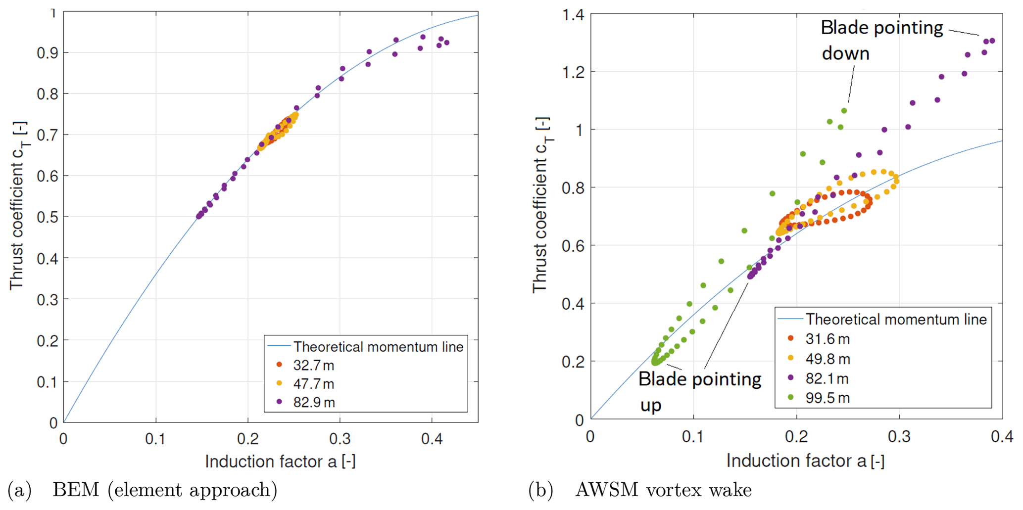
Figure 7 Comparison of post-processed AVATAR rotor simulation results in heavy shear (U=8 m s⁻¹, α=0.75) for several radial stations against the theoretical momentum line.

Acknowledging the fact that the vortex wake model does not obey the momentum equations as implemented in BEM theory, one may reflect on which shortcoming of BEM theory is responsible for this difference. Several assumptions are made in the derivation of BEM theory and an inventory was made of which specific violations of this theory occur in sheared inflow.

• Radial independence. The influence of neighboring elements and of the other blades is not taken into account and each annulus is treated separately. For a spanwise uniform circulation distribution it is acknowledged that intermediate trailed vorticity effects are absent, and as long as the loading differences between the blades are not significant this effect can be neglected as well. However in sheared inflow, even for a blade that is designed with uniform spanwise circulation distribution, a varying spanwise circulation distribution will result in trailed vorticity which violates the radial independence assumption.

• Axisymmetric or uniform inflow conditions. It is well known that BEM theory assumes steady inflow conditions, which relates to the variation in wind velocity along the longitudinal direction of the stream tube. In addition to this the derivation of the underlying one-dimensional axial momentum equation assumes that the inflow conditions are axisymmetric (or uniform) with respect to the stream tube considered. In sheared inflow conditions (or any other nonuniform inflow condition such as turbulent or waked inflow) it may be clear that this is not the case. It was shown previously that the Betz limit can be exceeded in nonuniform inflow conditions (Chamorro and Arndt, 2013). The implication of the violation of axisymmetric or uniform inflow conditions may differ between a BEM approach that solves the momentum equations “annulus averaged” (i.e., using one equation resulting in the same induced velocity for all the blades) or the more modern local approach that solves the momentum equation separately for each blade. In the latter case one may ask the question of what the azimuthal and radial extent of the stream tube is that balances the force exerted by a blade.

Further consideration of the second violation aspect triggered the idea to distinguish between the wind velocity used in BEM for the purpose of evaluation of the sectional force (U_e, blade element equations) and for the determination of induced velocity (U_m, momentum equations). See also the axial momentum equation (Eq. 2) below (for the sake of simplicity the tangential induction and a correction for the finite number of blades have been removed here).

$$\begin{array}{}\text{(2)}& \mathrm{2}a(\mathrm{1}-a)\mathit{\rho }{U}_{\mathrm{m}}^{\mathrm{2}}\mathrm{2}\mathit{\pi }r\mathrm{d}r=\sum _{B}c\mathrm{0.5}\mathit{\rho }{W}^{\mathrm{2}}{c}_l\left(\mathit{\alpha }\right)\cos \left(\mathit{\varphi }\right)\mathrm{d}r,\end{array}$$

where

$$\begin{array}{rl}& \mathit{\varphi }=\mathrm{atan}\mathrm{2}\left(U_{\mathrm{e}}(\mathrm{1}-a),\mathrm{\Omega }r\right),\mathit{\alpha }=\mathit{\varphi }-\mathit{ϵ}\mathrm{and}\\ & W=\sqrt{U_{\mathrm{e}}^{\mathrm{2}}(\mathrm{1}-a{)}^{\mathrm{2}}+(\mathrm{\Omega }r{)}^{\mathrm{2}}},\end{array}$$

with U_e (m) the wind speed used for the blade element equation, U_m (m s⁻¹) the wind speed used for the momentum equation, r (m) the radius of element considered, c (m) the local blade chord at radius r, ρ (kg m⁻³) the air density, W (m s⁻¹) the effective velocity at element, c_l (–) the lift coefficient, α (^∘) the angle of attack, ϕ (^∘) the inflow angle with respect to the rotor plane, Ω (rad s⁻¹) the rotor speed and ϵ (^∘) the twist-plus-pitch angle (and possible torsion deformation).

In this equation the blade element part is on the right-hand side, in which the wind velocity U_e is included through the effective velocity term W, the inflow angle ϕ and angle of attack α. The momentum part is on the left-hand side of Eq. (2). It is noted that in the so-called “annular average” BEM, the element forces are summed over the blades ($\sum _B$) and the corresponding annulus has a 360^∘ extent, resulting in a single axial-induction factor for all blades. The current “element” BEM implementation which is used here solves Eq. (2) for each blade separately (adjusting the annular volume correspondingly), resulting in different induced velocities for each blade element in an annulus.

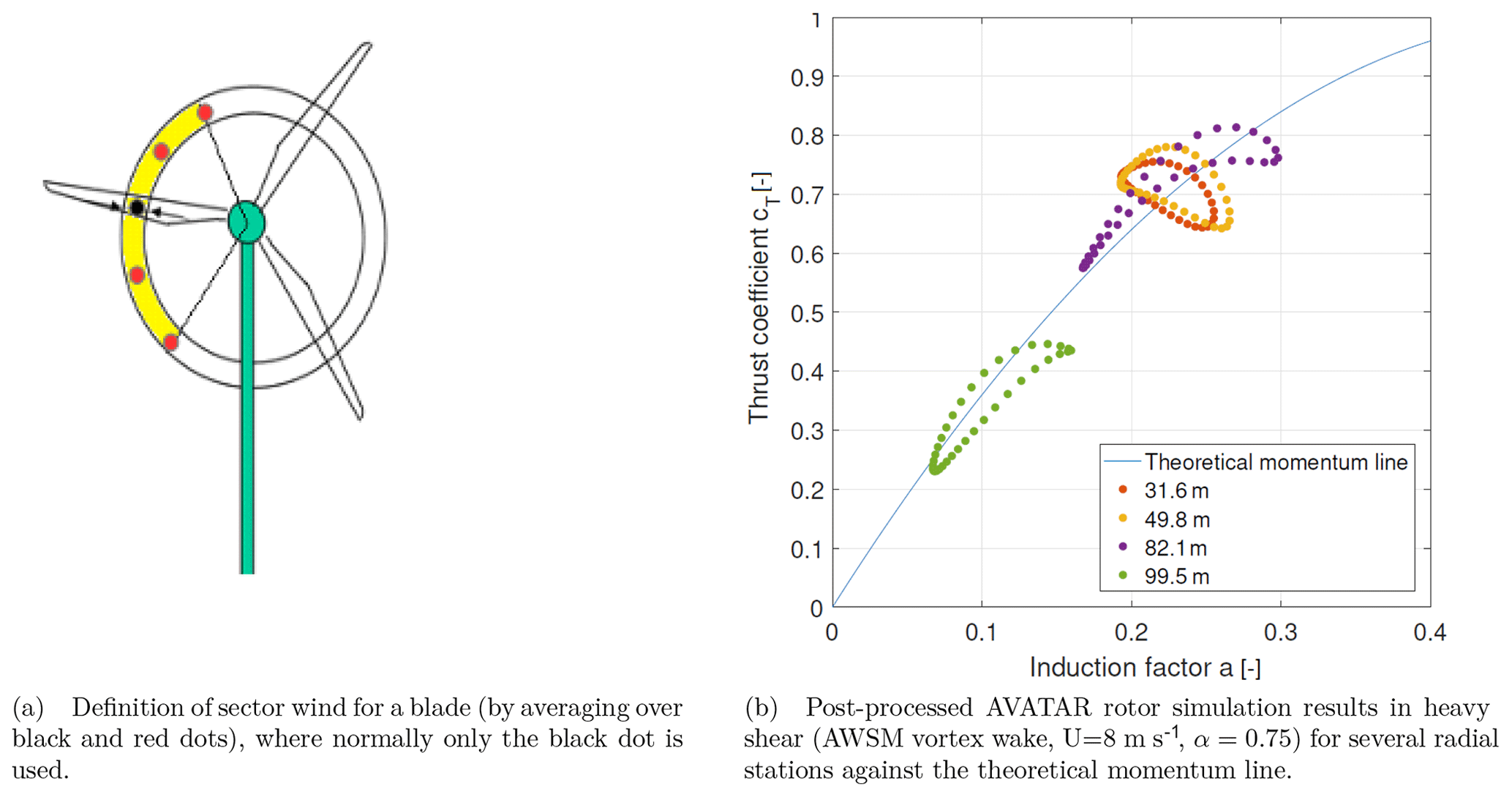
Figure 8 Definition of a sector-averaged wind and the effect of using this sector-averaged wind speed as reference wind speed for nondimensionalizing C_t and a.

Revisiting the idea to distinguish between the wind velocity used in BEM for the purpose of evaluation of the sectional force (blade element part) and the determination of induced velocity (momentum equations), it is clear that the local wind velocity acting at an element quarter or three-quarter chord point should be used for the first part. For the second part it could be argued to use a wind speed that is representative for the stream tube considered instead of a local point at the element center (as it is currently implemented). The question is how to define this stream tube and how to define a representative wind speed for it. Where a CFD or vortex wake simulation considers all spatial wind speed variations by means of a mesh, the momentum theory in BEM allows for only one. Effectively this is an inherent shortcoming of BEM and it could be argued we have arrived at a limitation that cannot be overcome. In a first attempt a stream tube is defined that considers an annular sector with azimuthal extent of 360^∘ divided by the number of blades, symmetrically distributed around the element of consideration. A simple five-point average is taken of the wind speed, with the five points equally distributed in the azimuthal direction at a spacing of 30^∘ for the current example with three blades (Fig. 8a). Application of this idea to the above-highlighted vortex wake simulation yields Fig. 8b, which shows an improvement in terms of agreement with the theoretical momentum line for the outboard sections (i.e., the results lie closer to this line). The inboard sections logically experience less inflow velocity variation due to shear and the sector approach appears not to improve the agreement with the theoretical momentum line.

Implementing the outlined approach in a BEM code has allowed for some further testing in sheared and turbulent inflow as illustrated in Fig. 9. In sheared inflow it is shown that induced velocity amplitudes and consequently the normal forces are more in line with the vortex wake modeling. The time trace in turbulent inflow (Fig. 9c) clearly illustrates the improved tracking of induced velocity of the sector wind approach, again very close to the vortex wake result except for the higher frequencies. The resulting integrated staircase plots (which are the result of the rain flow counting procedure for obtaining fatigue equivalent loads) show that application of a shed vorticity model (by means of the Beddoes–Leishman model ECNAero-BEM-BL instead of the default Snel model for unsteady airfoil aerodynamics) in combination with the sector approach (ECNAero-BEM-BL–sector) results in unsteady loading characteristics matching AWSM very well for this case.

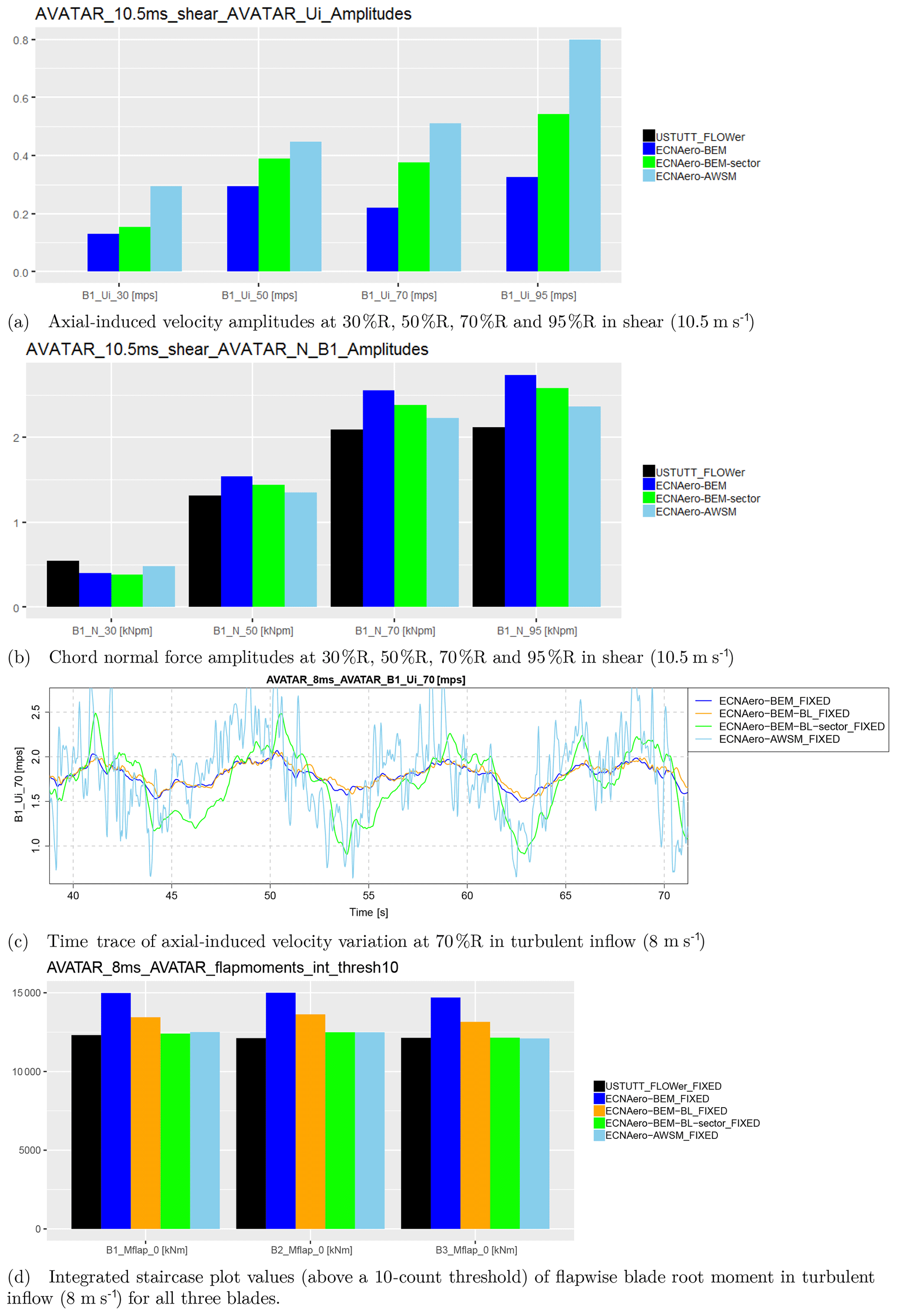
Figure 9 Comparison of sector wind BEM implementation (sector) to conventional BEM with Snel and Beddoes–Leishman (BL) modeling, vortex wake results (AWSM), and CFD (USTUTT_FLOWer) for selected AVATAR 10 MW rotor simulations.

It is recommended to have a more detailed look into the definition of a representative stream tube (e.g., varying azimuthal extent and position leading/lagging, averaging procedure) and run a variety of test cases (e.g., the cases were defined in Table 3 and the parametric shear investigation from Fig. 3, containing a variation in the number of blades), also to assure this procedure does not unintentionally cover up other effects such as shed and trailed vorticity variation. Reference is made to a recent publication (Madsen et al., 2020) that also addresses the issue of induction tracking by means of a new approach, now solving the BEM equations on a polar grid. This approach seems to resolve the damping of local induced velocities by the dynamic inflow model by decoupling the individual blade momentum equations on a grid. In the current formulation the momentum equations including the dynamic inflow term are solved locally but convergence is assessed by means of the annulus-averaged induction (average of the three local axially induced velocities in the case of three blades), which inherently introduces a coupling between the elements. This unwanted damping is counteracted by specifying a large number of subiterations per time step to ensure local convergence of the momentum equations (including dynamic inflow term), which is regarded as suboptimal.

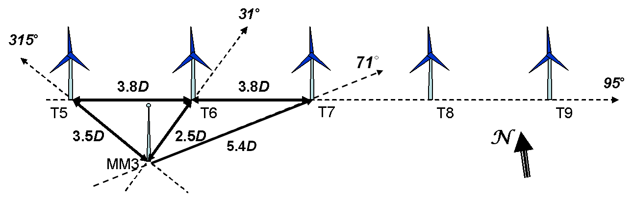
Figure 10 Main dimensions and directions in the EWTW farm. T5 to T9 are the turbine positions; MM3 indicates the measurement mast. Dimensions are expressed in rotor diameters D.

3 Validation against field data

Over a decade of measurements on 2.5 MW pitch-to-vane controlled research turbines are available from the EWTW test site (Machielse, 2006). In an attempt to validate fatigue load predictions against field data, these measurements were the subject of study.

3.1 Description of set-up

The EWTW farm (Eecen et al., 2006) that is the subject of investigation consisted of a row of five 2500 kW turbines with variable-speed pitch-regulated control. These turbines have a rotor diameter and hub height of 80 m and are placed at mutual distances of 3.8 rotor diameters (D). The farm is very well suited for investigation into effects at full scale because of its state-of-the-art turbines and the comprehensive and reliable measurement infrastructure for turbine and meteorological data.

The farm was orientated from west to east (95–275^∘); see Fig. 10. Turbine 6 has been instrumented with blade root strain gauges and hence is used for the load analysis. The wind characteristics are measured with the meteorological tower at 2.5 D southwest of turbine 6. This mast measures wind speed and direction at three different heights including hub height. Also, air pressure and temperature are measured at this height. More details can be found in the dedicated report (Machielse, 2006). The analyzed measurements at EWTW have been obtained from the period September 2004 until January 2012.

3.2 Data reduction

The SCADA and load signals of turbine 6 together with the meteorological data from mast 3 have been used for the analysis in this report. The 10 min statistics have been retrieved from the database. A wind direction criterium based on the undisturbed wind sector (between 110–140 and 200–250^∘) has been applied when retrieving the result from the database, resulting in about 100 000 samples. Further filtering out unwanted conditions (e.g., nonnumeric values; start-up, stop or idling conditions) resulted in about 25 000 remaining 10 min samples. The fatigue equivalent flapwise and edgewise moments of turbine 6 were acquired using a slope of 10 for the S–N curve (glass fiber). The rain flow counting method was applied to the raw signal, and the equivalent loads have readily been determined in the database according to IEC 61400-13 (International Electrotechnical Commission, 2001). Bin averaging is applied to the resulting datasets both in wind speed and turbulence intensity. The standard error of the mean within each bin is calculated using

$$\begin{array}{}\text{(3)}& S=\mathit{\sigma }/\sqrt{N},\end{array}$$

with S the standard error of bin average mean, σ the standard deviation over the bin data samples, and N (–) the number of samples per bin.

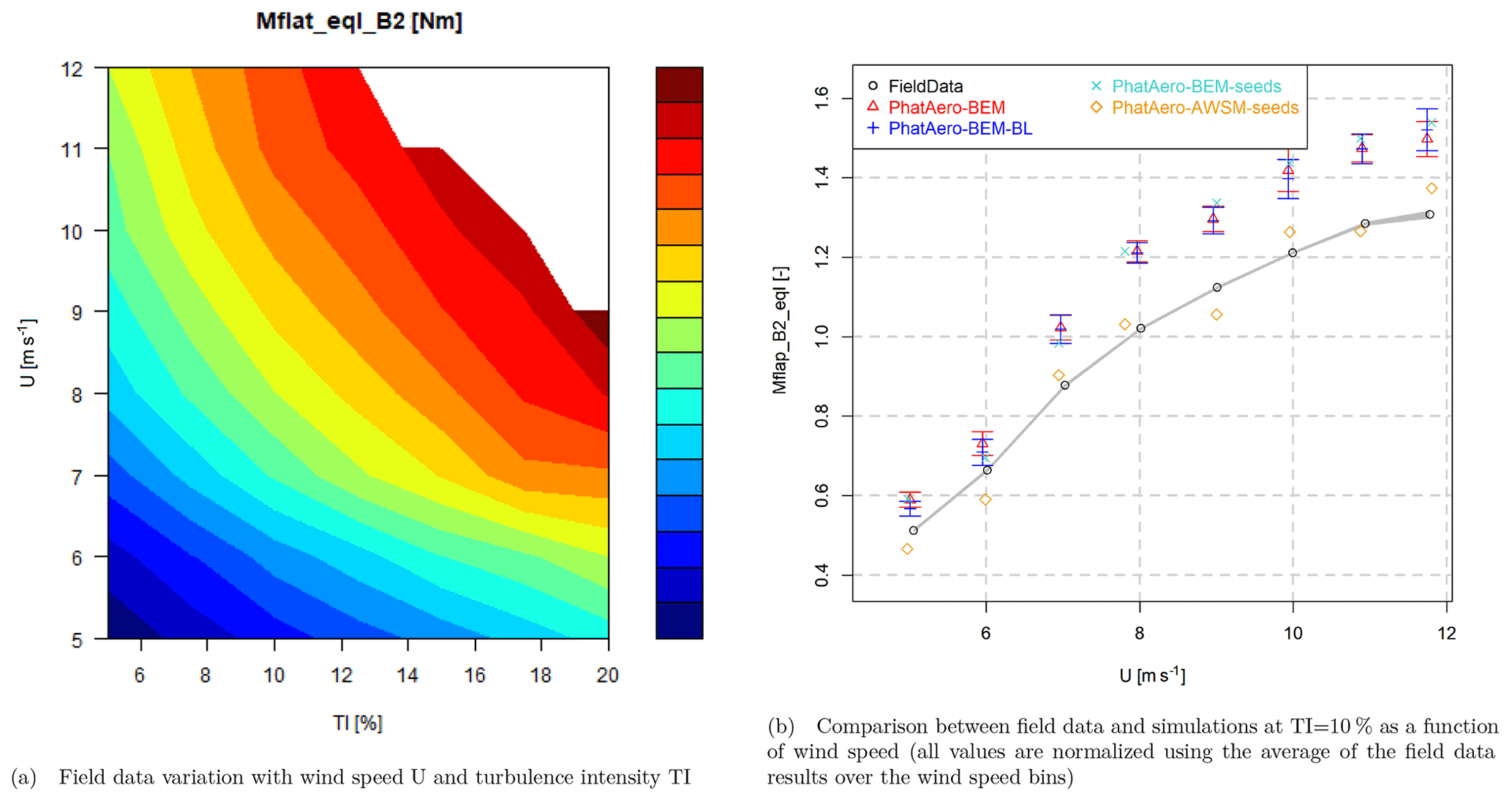
The resulting dataset from the filtering and binning has been visualized using contour plots as a function of turbulence intensity and wind speed, e.g., for the fatigue equivalent flapwise blade root moment in Fig. 11a.

Figure 11 Visualization of damage equivalent flapwise blade root moment.

3.3 Comparison to simulations

Using the bin-averaged operational conditions from the field data analysis, simulations are performed for all wind speed bins (5 to 12 m s ⁻¹) focusing on the 10 % turbulence intensity bin. A full aeroelastic model of the 2.5 MW research turbine was built using the PhatAero code as embedded in the FOCUS6 software, including mass, stiffness, control and aerodynamic details as disclosed by the turbine and blade manufacturer. In order to create a representative value for the fatigue loads, six 10 min seeds were created per wind speed bin using the TurbSim wind generator (Jonkman and Buhl Jr., 2006), making sure that the resulting turbulence intensity matched the specification from the field data analysis. Default IEC values were used for shear and turbulence spectra as these details were not available from the measurements. In view of the limited time, the number of vortex wake simulations (PhatAero-AWSM) was limited to only a few seeds. For each wind speed considered, a representative seed was selected which matched the statistics and equivalent loads compared to the average over the six seeds for each wind speed bin as well as possible. For these specific seeds, the rotational speed variations resulting from the BEM simulations were recorded and fed to the AWSM simulations to have a consistent comparison between them. The settings were similar to the settings as reported in Sect. 2.1.3. The statistics and equivalent loading of all simulation results were obtained after skipping the first 100 s, which is regarded as initialization time, hence using the remaining 500 s. Similar to the binning of the measured 10 min statistics, the simulation results were averaged over the six available seeds for each wind speed bin. In addition the standard error was calculated in accordance with Eq. (3). To comply with confidentiality requirements, the loads and power have been normalized using the average of the field data results over the wind speed bins. The main comparison plot result is given in Fig. 11b. The results for the elected representative seeds are also given, indicated by PhatAero-BEM-seeds and PhatAero-AWSM-seeds.

The equivalent loading for the flapwise moments is overpredicted around 15 % by the BEM simulations (averaged over all seeds and blades), where the AWSM vortex wake simulations are very close to the measurements (−1 % averaged over all seeds and blades). A similar conclusion can be drawn for the standard deviation. This trend is similar to the results obtained from the comparison to CFD. Although the absolute difference between measurements and BEM simulations increases with wind speed, the relative difference in terms of percentage remains largely constant over the wind speed range. It is noted that, although not shown here, the averaged flapwise moments are slightly (<5 %) underpredicted by the simulations, where they agree well between the different simulation settings.

Application of the Beddoes–Leishman model (PhatAero-BEM-BL), which adds modeling of shed vorticity effects, reduces the difference with the measurements only slightly (around 1 % decrease). This is not in agreement with the comparison to CFD featuring the 10 MW AVATAR rotor, which showed the modeling of shed vorticity to reduce the difference between BEM and high-fidelity models significantly. It is unclear at this point what is causing the discrepancy between these observations.

Care should be taken drawing conclusions on the basis of these results, since it is felt that comparing aeroelastic simulations to field data is subject to many uncertainties (inflow, control, model data, compensating errors, etc.) that cannot easily be verified. A great effort was made however to eradicate most of these, e.g., by running simulations for a large number of seeds and using a large number of measurement samples. It is recommended to set up a dedicated field test in an effort to further reduce the underlying uncertainties. Here one can think of using nacelle lidar to characterize the inflow conditions in more detail for synthetic wind field creation in combination with unsteady pressure sensors to measure sectional aerodynamic loading. In addition it is recommended to include more vortex wake simulations (similar to the number of BEM simulations) to better quantify the difference between these code types. More details about the comparison to field data can be found in the dedicated report (Boorsma, 2019).

4 Impact on IEC design load calculations

Both vortex wake and BEM-based models describe the blade aerodynamics on the basis of sectional properties of the airfoils, and both with options to account for dynamic stall effects and corrections for the effects of rotation. This means that the main difference between these model types is the description of the rotor wake aerodynamic effects, which is done in far more detail by the vortex wake methods. An inventory is made showing from which conditions and IEC load cases (International Electrotechnical Commission, 2019) a difference is to be expected from vortex wake instead of BEM-based models. Scoping analyses have been performed with both a BEM and vortex wake code for an entire fatigue load set to verify the differences.

4.1 Conditions and IEC load cases

Load case conditions for which vortex wake descriptions are expected to give more realistic predictions than BEM-based models can be categorized by recalling the violations of the underlying BEM assumptions. Here we can mention nonuniform inflow conditions, unsteady disk loading, yaw misalignment, asymmetric blade loads (e.g., pitch actuator failure), spanwise circulation variation (e.g., distributed control, tip effect), radial induction and nonplanar blade geometries (e.g., sweep, winglet). Although engineering sub-models are developed to overcome most of these limitations, the uncertainties accompanying these are often large (Boorsma and Schepers, 2018). Eventually it depends on the turbine under consideration (e.g., operating axial-induction factor, blade shape), if the load cases listed here give structural loads that are significant for the design. Based on the conditions described here the following load cases from IEC 61400-1 (International Electrotechnical Commission, 2019) are considered for evaluation with a vortex wake model.

• Fatigue load cases. Following the comparison results in this paper, normal power production (DLC1.2) is a candidate for evaluation with a vortex wake model. In general the wake descriptions with vortex wake methods really make a difference if the induced velocities at the rotor are a significant fraction of the ambient wind velocity. This means for example that for a wind near or above the cutout conditions the wake effects have a very small contribution. Scoping analyses on the production load cases are reported in Sect. 4.2. In addition to DLC1.2, operation with failed yaw or failed pitch that is not (yet) detected (DLC2.4) can be considered due to the asymmetric loads over the rotor.

• Extreme load cases. Prior to analyzing some of the ultimate load cases with vortex wake programs, it is recommended to first analyze these load cases with a BEM-based program to explore which of the load cases are design-driving. This holds especially true for the cases with longer simulation time. Already it is envisaged that DLC1.4 & DLC3.3 extreme coherent gust with direction change (ECD) (unsteady asymmetric disk loading) and DLC1.5 extreme wind shear (EWS) (nonuniform inflow conditions) calculation with vortex wake models may be more realistic. Although wake effects are anticipated to be small in DLC6 due to the parked rotor conditions, spanwise circulation variation can still have an impact on the loading.

  One may expect that DLC1.3 extreme turbulence model (ETM) may be considered for calculation with a vortex wake model because DLC1.3 tends to give design-driving loads and because the extreme turbulence model may give highly nonuniform rotor disk loading that is quite unsteady at the same time. Besides the large amount of CPU that is needed for the various 600 s calculations, one may argue that using a vortex wake model does not make much sense because eventually the turbulence level of the extreme wind speed model (EWM) has to be scaled such that the extreme blade root bending moments and the largest blade tip deformations match with the 50-year extrapolated values from DLC1.1. This means that if DLC1.3 is calculated with a vortex wake model instead of a BEM-based model, one may end up with a different scaling of the ETM. At least for the blade root bending moments and for the tip displacements, this would end up with nearly similar values. However, some differences may appear for the loads in the other wind turbine components.

4.2 Fatigue load set

Scoping analyses have been performed with both BEM-based programs and the vortex wake code AWSM for an entire fatigue load set featuring the 10 MW AVATAR turbine. Design class IA was used which has a reference wind of 50 m s⁻¹, a Weibull average wind of 10 m s⁻¹ and a characteristic turbulence level of 16 %. The wind is modeled with a power law for the vertical shear with an exponent of 0.2, although for offshore wind turbines the IEC recommendations prescribe a vertical shear exponent of 0.14. The inclination of the ambient wind is set to zero. The wind velocities for which the turbine is in operation range from 4 m s⁻¹ to 25 m s⁻¹ while for each wind (with 1 m s⁻¹ intervals) three calculations are performed with different wind stochastics. For these three calculations the yaw misalignment has values of −8, +8 and 0^∘. The turbulence applies to the frequency spectrum of Kaimal, and for each wind velocity another random seed was used. In comparison to the rigid rotor calculations which were compared to CFD, the aeroelastic turbine in Phatas was modeled including all flexibilities (e.g., tower and blades) and active controller as defined in the EU AVATAR project. The time increment was set to 0.05 s. Simulations were performed with PhatasSV, Phatas-BSV, PhatAero-BEM and PhatAero-AWSM.

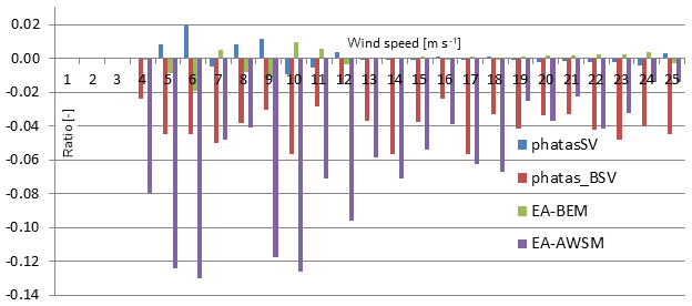
Figure 12 Blade root flap fatigue loading ratios relative to the average over PhatasSV and PhatAero (EA)-BEM as a function of wind speed.

Although the resulting load characteristics were also compared for the tower and nacelle, the results of the flapwise blade root moments are given in Fig. 12. This figure shows the largest reductions of the vortex wake model in sub-rated conditions featuring higher axial-induction factors, in agreement with the observations from Sect. 2 for the comparison to CFD. For wind velocities rated above, the fatigue predictions with blade shed vorticity model (Phatas-BSV) are close to the AWSM vortex wake simulations. The same trends roughly hold for the tower base tilt moment.

Although only a set of normal production load cases is calculated with AWSM, it is expected that the reduction in overall fatigue damage by using the program AWSM may be up to 5 % for the AVATAR rotor. This is a consequence of the relatively large contribution of the higher wind speeds to the overall fatigue. The blade shed vorticity algorithm gives an overall fatigue load reduction of about 2 % compared with the BEM-based programs without this blade shed vorticity contribution. It is noted that the given percentages are obtained for the AVATAR turbine featuring a low induction rotor and may vary depending on the design-operating axial induction. For more details please consult the dedicated report about the IEC load set survey (Lindenburg, 2019).

5 Conclusions

Making a meaningful comparison between CFD and lifting-line codes has appeared to be quite a challenge in terms of inflow alignment. However a promising engineering approach was devised which allowed successful comparisons in the time domain between these code types. A test matrix was defined covering representative operational and inflow conditions, bearing the CPU requirements in mind. The fatigue load reduction from BEM to vortex-wake-type codes as observed in the EU AVATAR project has been confirmed by these dedicated CFD simulations. This is partly explained by the shed vorticity effect which is implicitly included in the vortex-wake-type codes, but poor tracking of wind variations by induction for BEM remains an issue. It is recommended to further study this aspect to further reduce uncertainties in BEM modeling. In addition to that very similar results were obtained between several vortex wake codes originating from different institutions. A variety of load cases have shed more light on this subject, showing a correlation of the observations with axial-induction factor.

In addition to the comparison against CFD simulations, a validation was made against measured fatigue loads of a real turbine at the EWTW test site. Over 7 years of measurements were analyzed to obtain relevant statistics over one hundred thousand 10 min samples, of which about 25 000 remained after filtering out unwanted conditions. The data were bin averaged with respect to turbulence intensity and wind speed, after which dedicated simulations for each wind speed bin were run at 10 % turbulence intensity. The resulting load comparison shows BEM to overpredict the fatigue equivalent flapwise blade root moments, where a vortex wake model comes closer to the measurements. However care should be taken drawing conclusions, since it is felt that comparing aeroelastic simulations to the field dataset is subject to many uncertainties (inflow, control, model data, compensating errors, etc.) that cannot easily be verified. A great effort was made however to eradicate most of these, e.g., by running simulations for a large number of seeds and using a large number of measurement samples. It is recommended to set up a dedicated field test in an effort to further reduce these uncertainties, allowing a better validation. Here one can think of using nacelle lidar to characterize the inflow conditions in more detail for synthetic wind field creation in combination with pressure sensors to measure sectional aerodynamic loading.

An inventory is made showing from which conditions and IEC load cases a difference is to be expected from vortex wake instead of BEM-based models. Based on past experience it is anticipated that differences are to be expected in nonuniform and yawed inflow conditions, especially when operating in high thrust coefficients. Scoping analyses have been performed with both a BEM and vortex wake code for an entire fatigue load set to verify the differences. Although only a set of normal production load cases is calculated with a vortex wake code, it is expected that the reduction in overall fatigue damage by using a vortex wake program may be up to 5 % for the relatively low-induction AVATAR rotor, of which about half was attributed to shed vorticity effects. A more extensive exploration of design load calculations and the added value of vortex wake calculations is yet to be performed, focusing not only on fatigue loads but also on extreme loads and power production.

Concluding, a very successful validation of lifting-line codes against CFD and field data has been performed. A validation study similar to the cases studied in this project in a physical wind tunnel is recommended as “proof of the pudding”.