the Creative Commons Attribution 4.0 License.
the Creative Commons Attribution 4.0 License.
 | 22 Mar 2021
Power fluctuations in high-installation- density offshore wind fleets
Matti Juhani Koivisto
Poul Sørensen
Philippe Magnant
Detailed simulation of wind generation as driven by weather patterns is required to quantify the impact on the electrical grid of the power fluctuations in offshore wind power fleets. This paper focuses on studying the power fluctuations of high-installation-density offshore fleets since they present a growing challenge to the operation and planning of power systems in Europe. The Belgian offshore fleet is studied because it has the highest density of installation in Europe by 2020, and a new extension is expected to be fully operational by 2028. Different stages of the future installed capacity, turbine technology, and turbine storm shutdown technologies are examined and compared. This paper analyzes the distribution of power fluctuations both overall and during high wind speeds. The simulations presented in this paper use a new Student t-distributed wind speed fluctuation model that captures the missing spectra from the weather reanalysis simulations. An updated plant storm shutdown model captures the plant behavior of modern high-wind-speed turbine operation. Detailed wake modeling is carried out using a calibrated engineering wake model to capture the Belgium offshore fleet and its tight farm-to-farm spacing. Long generation time series based on 37 years of historical weather data in 5 min resolution are simulated to quantify the extreme fleet-level power fluctuations. The model validation with respect to the operational data of the 2018 fleet shows that the methodology presented in this paper can capture the distribution of wind power and its spatiotemporal characteristics. The results show that the standardized generation ramps are expected to be reduced towards the 4.4 GW of installations due to the larger distances between plants. The most extreme power fluctuations occur during high wind speeds, with large ramp-downs occurring in extreme storm events. Extreme ramp-downs are mitigated using modern turbine storm shutdown technologies, while extreme ramp-ups can be mitigated by the system operator. Extreme ramping events also occur at below-rated wind speeds, but mitigation of such ramping events remains a challenge for transmission system operators.
- Article
(2557 KB) - Full-text XML
- BibTeX
- EndNote


Belgium has adopted the target of a 65 % reduction of greenhouse gas emission levels by 2050, a less ambitious target than the European target of 80 % by 2050. Nevertheless, Belgium is expected to increase the share of renewable energy sources, with an expected increase in wind energy share of between 37 % and 44 % by 2050 (Mikova et al., 2019). The Belgian offshore wind power fleet will be, by the end of 2020, one of the areas with the highest installation density in the North Sea (approximately 10 MW km−2, while the average is 6.6 MW km−2), with an installed capacity of circa 2.3 GW over a marine area of circa 225 km2 in proximity to the Netherlands. Furthermore, the planned expansion of the Belgian offshore fleet will bring the capacity up to between 4.0 and 4.4 GW by 2028 (Elia, 2017, 2019). Previous studies of the impact of the Belgian offshore fleet in its energy system exist: Elia (2018) studies the impact of storm and ramping events on the system imbalances, while Buijs et al. (2009) investigate the required investment by the Belgium power system for integrating the 2.3 GW of offshore wind.
Geographical smoothing of the fleet-wise offshore wind production is expected in the 4.4 GW scenario as the new plants are located further apart from the existing fleet and due to the decrease in correlation between power productions from plants further apart. Several studies explore the effects of the distance among wind power plants in the fleet/portfolio wind production such as Santos-Alamillos et al. (2017), Tejeda et al. (2018), Roques et al. (2010), and Koivisto et al. (2016). Additionally, the expected increase in rotor diameter, hub height, and general improvements of wind turbine technology can have a smoothing effect in fleet-wise wind power production (Koivisto et al., 2019b).
The distribution of the fleet-level power fluctuations is necessary to understand and model the impact of the future expansions of the Belgian offshore fleet into the Belgian energy system (Huber et al., 2014). Holttinen et al. (2011) present a detailed analysis of the impacts of large amounts of wind power on the design and operation of power systems. Holttinen et al. (2016) show that characteristics of variability and uncertainty of wind power are an important input for wind integration studies, with impacts on system-balancing and grid-reinforcing needs. A long-term dynamical simulation of the offshore wind power generation is required to assess the impact of the extreme power fluctuations in the energy system (Pfenninger, 2017).
The purpose of this paper is to quantify the distribution of ramp rates as a measure for power fluctuations when extending the offshore wind capacity in Belgium. This research proposes a methodology for simulating wind power production time series and performing a validation using operational measurements on the 2018 fleet. This paper concentrates on the simulations of the time series of offshore wind generation for several scenarios. The simulated time series can be used as inputs in power and energy system impact analyses, but a detailed model of the energy system is not in scope. The hypothesis of this study is that power fluctuations in the Belgian offshore wind fleet will be reduced by a combination of increased spatial smoothing (larger distances between new installations) and the use of turbines with controlled high-wind-speed operation.
This paper includes several novel methodologies that address current gaps in large-scale offshore wind generation simulation: first, it presents a Student t-distributed wind speed fluctuation model and its validation. This model is based on the work by Mehrens et al. (2016) that shows that wind speed fluctuations are non-Gaussian and by Koivisto et al. (2016) that models the error terms in a multivariate autoregressive model with a marginally Student t-distributed Gaussian copula. Second, this paper presents an update to the hysteresis plant storm shutdown model by Litong-Palima et al. (2016) and its validation. Third, the methodology for simulating power production takes into account wake losses including farm-to-farm interactions. Fourth, a detailed validation of the results in terms of capacity factors (CFs), high-wind-speed operation, power fluctuations, and spatial correlations for the existing fleet demonstrates the simulation capability of the model chain used. Additionally, this paper has practical significance because it illustrates how the proposed methodology can be used to accurately predict the distribution of the fleet-level power fluctuations including its most severe extremes.
Large-energy-system modeling is required in order to design, plan, and adapt to the future transition to greener technologies. Pfenninger et al. (2014) present a literature review on large-energy-system models and identify the main challenges of large-energy-system simulations as (a) temporal–spacial resolution, (b) uncertainty and transparency, (c) growing complexity of interconnected energy systems with a diverse mixture of technologies, and (d) integrating the impact of policy and other human behaviors. Furthermore, Engeland et al. (2017) present a review of the modeling approaches for variable renewable energy (VRE, i.e., wind and solar). This review highlights the different methodologies required to simulate the generation of a wind power fleet as a time series. Holttinen et al. (2016) highlight the importance of modeling geographical smoothing when analyzing variability and uncertainty of wind power in system integration studies. The most common approaches are (1) stochastic time series simulations, (2) simulations based on meteorological reanalysis simulations, and (3) combinations of the two.
Stochastic time series simulation of fleet-level wind power production has been used in several studies. Ekström et al. (2017), Koivisto et al. (2016), Klöckl and Papaefthymiou (2010), and Olauson et al. (2017) are examples of applications and implementations of extended vector autoregressive models to simulate VRE generation time series. Sørensen et al. (2002) introduced the use of a stochastic time series model for simulating the wind speed fluctuations by combining the Kaimal turbulent spectra (for fluctuations within 10 min resolutions) with a low-frequency spectra designed to simulate the weather patterns in larger-scale fluctuations. All these simulation approaches rely on stochastic time series models to capture the auto- and cross-correlations of the power time series at multiple locations. Some of these stochastic models are fitted on measured historical data and have the limitation of not being able to predict the production time series on wind power fleets with different characteristics (i.e., installed capacity, locations, turbine types) from the original data. Direct stochastic power simulations have the advantage of not requiring the simulation of wind speeds, but instead they rely on empirical transformations of the data to correct for the non-stationarity, non-Gaussianity, and correlation structure of power fluctuations. Fertig (2019) introduces an empirical model to apply stochastic models to different installed capacity and locations.
Weather-driven wind power time series generation simulations consist in modeling the wind production as driven by wind speed time series obtained from (1) meteorological reanalysis datasets such as ERA-Interim (Dee et al., 2011), MERRA (Gelaro et al., 2017), or ERA-5 (Hersbach et al., 2020) and (2) Weather Research and Forecasting (WRF) model simulations (Skamarock et al., 2008). Example applications of weather-driven wind generation simulations can be read in Nuño et al. (2018), Olauson and Bergkvist (2015), Marinelli et al. (2014), Leahy and Foley (2012), Von Bremen (2010), Staffell and Pfenninger (2016), Thomaidis et al. (2016), and Staffell and Pfenninger (2018). The main advantages of using meso-scale weather-driven generation simulations are as follows. (a) The simulations rely on the predictions of wind speeds and wind directions, among other meteorological parameters, and therefore have physical consistency between different locations and times. (b) The simulations can be performed on any combination of installed capacity, locations, and wind turbine technologies. (c) The simulations can be extended to cover larger periods of time, which will be necessary for reliability or extreme event probability estimations (Pfenninger, 2017). The disadvantages are as follows. (a) Low spatiotemporal resolution means that not all the variability in the wind speed is captured. Hourly resolution is widely used in most studies, but simulations can be carried out with 10 min resolutions or more but with a significant additional computational costs (Liu et al., 2011; Talbot et al., 2012). Spatial resolution of 10 km is widely used in wind energy (González-Aparicio et al., 2017), but WRF simulations can be performed in up to 100 m × 100 m areas (Liu et al., 2011; Talbot et al., 2012), while modern reanalysis datasets have resolutions between 10–75 km, (González-Aparicio et al., 2017; Olauson, 2018). (b) Simulated time series are smoother than measurements because the weather models tend to filter the high-frequency oscillations from the signals in order to ensure convergence. (c) Due to the coarse temporal resolution, turbulence spectra are missing, which are necessary to simulate with higher resolutions than 10 min.
Stochastic models are designed to capture the missing wind speed fluctuations. Veers (1988) demonstrated that time series interpolated from a grid of correlated time series produce a decrease in the apparent spectra, and they proposed a methodology to add missing fluctuations to compensate for this effect. Larsén et al. (2012) report the missing spectra in WRF with respect to measurements and analyses the implications for extreme wind speed estimation. Larsén and Kruger (2014) introduce and apply the spectral correction for WRF in South Africa, while Sørensen et al. (2018) apply it in the 2025 wind power scenario in South Africa. Koivisto et al. (2020) calibrate the parameters of the stochastic wind speed fluctuation model based on measurements. Mehrens et al. (2016) present non-Gaussian distribution of wind speed fluctuations in WRF and in measurements in offshore met mast sites. Olauson et al. (2016) present an empirical approach to model the fluctuations by introducing a machine learning regression model for the volatility and optimizing the phase angles between the different Fourier modes of the fluctuations to capture auto- and cross-correlations. For reference, Liu et al. (2017), Kiviluoma et al. (2016), and Apt (2007) present modern experimental spectra of wind power generation.
The wake behind the turbine is a flow characterized by a decrease in the mean wind speed and an increase in the turbulence downstream. Porté-Agel et al. (2020) provide a review of the work on the wake modeling and measuring field. In summary, the wakes translate into a lower power production on turbines operating in the wake of other turbines. Wind turbine wakes recover as a function of the distance from the turbine, which causes the effect to be most important when turbines are closely spaced. As turbines in the Belgian fleet are tightly spaced, significant wake effects are expected.
Farm wake is the aggregated effect of the wakes from all the turbines in a farm on the turbines in a nearby farm. Such effects have been reported to retain wind speed deficits of up to 2 % at downstream distances between 20–60 km (Volker et al., 2017). This distance of expected influence of farm wakes depends on the plant size, number of turbines, and atmospheric boundary layer stability (Porté-Agel et al., 2020). Farm effects are important in this study because of the proximity between the offshore wind plants in the Belgian waters.
Agora Energiewende et al. (2020) and Volker et al. (2017) report an expected capacity factor of around 30 %–50 % for areas with high power density (10 MW km−2) spreading over areas between 1–10 km2, depending on the wind resource in the region. Note that these capacity factors include the intra-farm (wakes of turbines in the same farm) and farm-to-farm wake losses.
3.1 Future wind turbine technology and installed capacity scenarios
To build representative scenarios for 2025–2028, the trends in offshore turbine technology are analyzed in terms of turbine capacity, specific power (ratio between rated power and rotor area), and hub height; see Fig. 1. The trends combine the current turbines installed or planned in Belgium and the Netherlands, the technology projections (Danish Energy Agency, 2020), and the commercial wind turbine prototype information available on the main wind turbine manufacturer's websites. Figure 1 shows that there is a linear trend in increasing hub height and turbine capacity, while the specific power tends to follow a cyclic trend with a linear increase followed by a drop in specific power. Two turbine technology scenarios are propose in this paper (Tech A and Tech B); both scenarios assume the same rated power but different specific power. The Tech A turbine has a high specific power, while Tech B has low specific power. The range of difference in rated power from different manufacturers is expected not to have significant impact on the results presented in this paper.
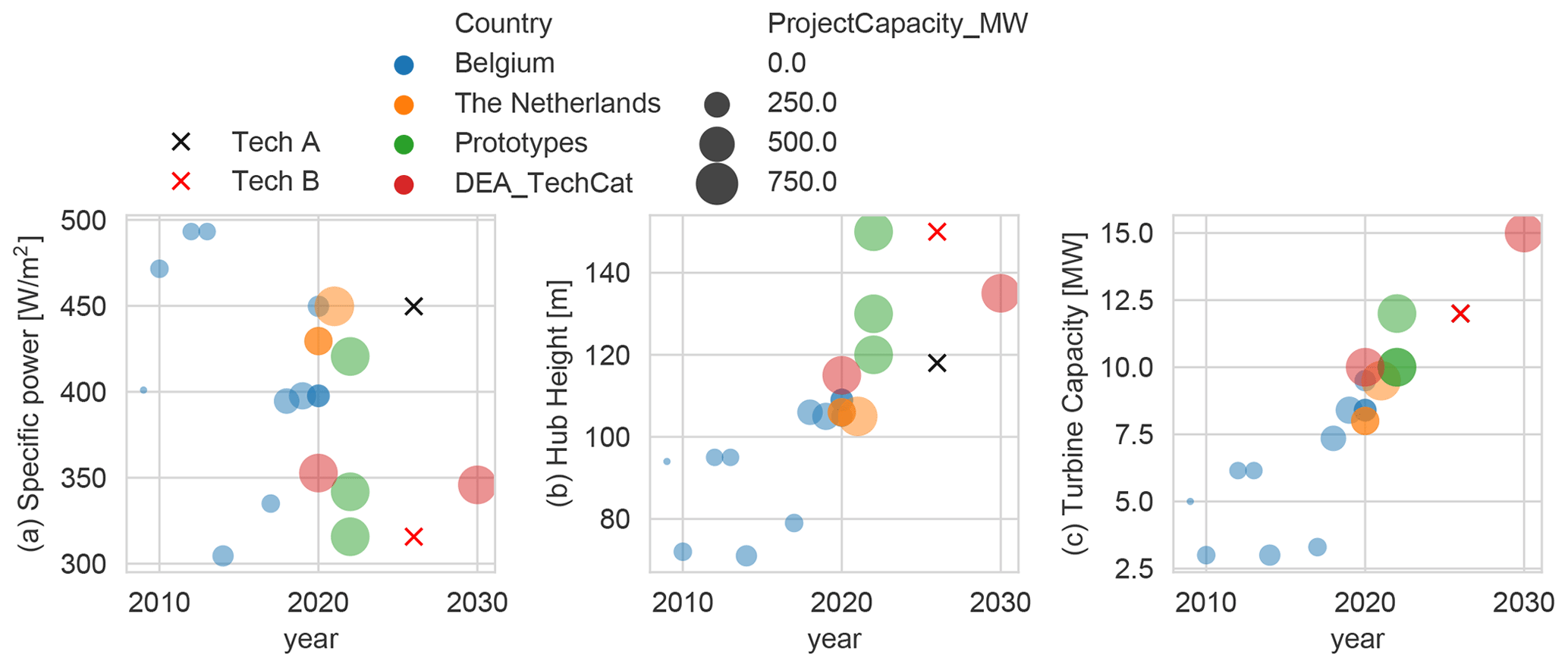
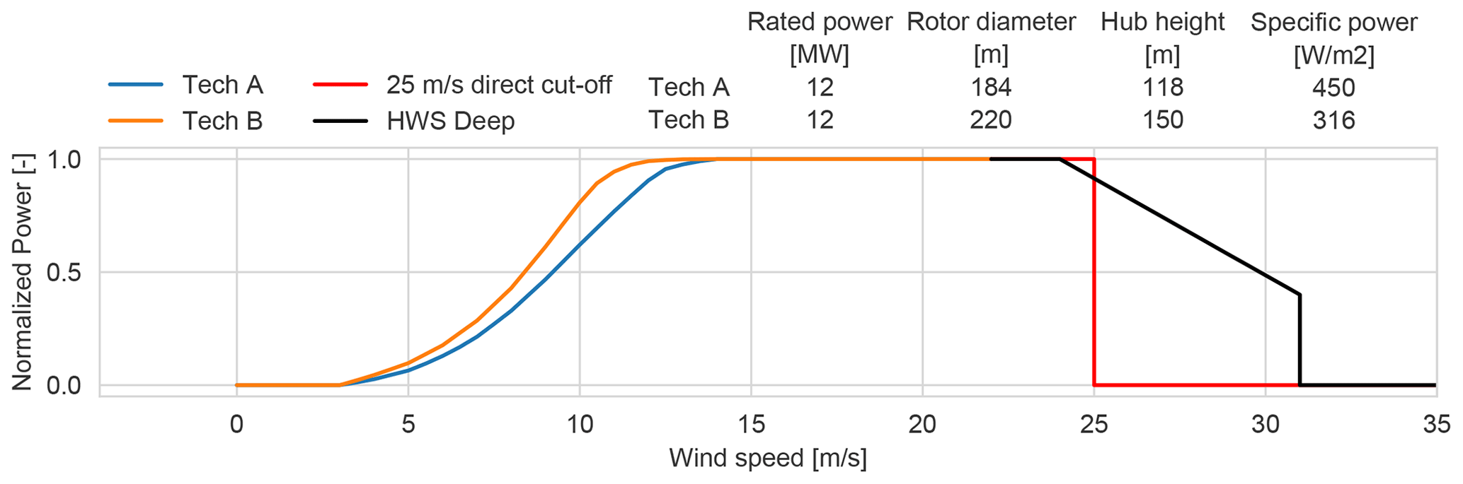
Figure 2Power curves and technical parameters for assumed technology and storm shutdown scenarios.
The power curves from the two turbine technologies are approximated based on the specific power, using the power and thrust coefficient curves of large rotors in DTU Wind Energy's database. Modern wind turbines are offered with high wind speed operation, which consists in extending the cut-off wind speed and implementing different control strategies to reduce the aeroelastic loads on the turbine components and hence reduce the power production. In this study a generic high-wind-speed operation technology (HWS Deep) is compared with respect to the traditional cut-off wind speed at 25 m s−1; see Fig. 2. The HWS Deep type represents modern turbines designed to continue operation at high wind speeds and mitigate the ramping due to storm shutdowns. High-wind-speed operation technology is commercially available, but every manufacturer uses a different control strategy, which results in differences in the power curves at high wind speeds. The HWS power curve presented in Fig. 2 is proposed to have a manufacturer agnostic HWS technology model. In this paper there are four turbine-curtailment technology scenarios: Tech A with 25 direct cut-off, Tech A with HWS Deep, Tech B with 25 direct cut-off, and Tech B with HWS Deep.
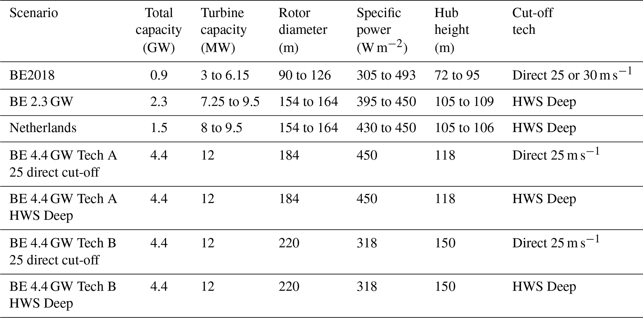
Future installation development is split into three scenarios or stages: BE2018 with 0.9 GW represents the validation dataset in which 4 years of operational data are available, and BE 2.3 GW consists of the plants in BE2018 and the plants to be commissioned by 2020, BE 4.4 GW consists of the plants in BE 2.3 GW and future extension; see Fig. 3 and Table 1. The turbine and layout used in the plants in the BE 2.3 GW scenario are known (Sørensen et al., 2020). The BE 4.4 GW scenario is studied by varying the turbine and shutdown technology for the additional 2.1 GW of installations. The plant layout in BE 4.4 GW is generated by maximizing the spacing between the turbines needed to reach the full installed capacity. Furthermore, the offshore fleet in the Netherlands (1.5 GW to start operating by 2020) is also modeled in the BE 2.3 GW and 4.4 GW scenarios because of its proximity.

Figure 3Plant and turbine locations for the different stages of offshore wind installations.
Table 1Plant and turbine characteristics for the different stages of offshore wind installations. Characteristics are given for the added turbines with respect to the previous stage of installation except for total capacity. The Dutch plants are taken into account when modeling external wake impacts on the Belgian fleet. Note that the actual turbines and plant layouts for the BE2018, BE 2.3 GW, and Netherlands scenarios were used.
3.2 Modeling
This section describes all the methodology used to produce the power time series simulations, including wake modeling, wind speed time series generation, and wind plant storm shutdown modeling implemented in CorRES (Correlations in Renewable Energy Sources) (Koivisto et al., 2019a, 2020). CorRES uses meso-scale weather-driven renewable energy generation and has three sub-models: (1) meso-scale weather data and interpolation, (2) a wind speed fluctuation model, and (3) a wind-to-power model which includes wake modeling and a dynamic storm shutdown model.
3.2.1 Wind speed time series simulation
Wind speed time series for multiple locations are simulated by combining a pre-computed database of meteorological reanalysis simulations (uWRF) and a stochastic model to compensate for the missing fluctuations (δu), see Eq. (1), where xj is the location of plant j at a given time, t. The following methodology is based on Sørensen et al. (2008) and Koivisto et al. (2020).
CorRES meteorological reanalysis data are obtained by running WRF (Skamarock et al., 2008) to downscale the ERA-Interim reanalysis data (Dee et al., 2011) at a 10 km × 10 km × 1 h resolution. Nuño et al. (2018) give a detailed description of the WRF simulations used in this paper. The model results are stored at multiple heights above ground (50, 80, 100, 120, 150 m). Linear interpolation in horizontal coordinates and piecewise power-law interpolation are used to obtain the time series on a given farm center position.
The stochastic model used to compensate for the missing high-frequency spectra and the turbulence contribution to the inter-time-step variability in the wind speed signals is characterized by its power spectral density (PSD), Sjj(f); see Eq. (2). In this equation the coefficient a1 is a parameter of the spectra, while f0 controls the lower frequency from which variability will be added. Koivisto et al. (2020) report the calibration of a1 and f0 to wind speed measurements in Høsøre, Risø, and Cabauw. The fluctuation spectra are designed to capture the full-range spectra as reported by Larsén et al. (2016) with the addition of the f0 parameter, used to minimize the low-frequency modification of the WRF time series.
Since the simulations represent several locations, the coherence between the wind speed fluctuations (on a given frequency) between two locations is specified by the coherence function, γjk(f), in Eq. (3), where Ajk is the decay coefficient, djk is the distance between the locations, and ujk is the mean wind speed at the locations.
The decay coefficient is defined as a function of the streamwise (As) and transversal (At) components in Eq. (4), by projecting them along the direction of location alignment, αjk is the direction of alignment, and θjk is the mean wind direction at the locations. Sørensen et al. (2008) report calibrated values of At=4 and based on multiple location measurements in Høsøre.
The spectral matrix, S, is computed using the cross-spectra and coherence functions on a discretized frequency bin (with center frequency fm), for every pair of location j and k; see Eq. (5).
The time series generation methodology presented in Veers (1988) is used. The spectral matrix is approximated by a real, lower triangular matrix H, such that . This matrix is computed in an iterative manner following Eq. (6).
Finally, the complex Fourier coefficients of the wind speed fluctuations, Vj(fm), are computed as a linear combination of the weights given by H(fm) and a series of independent, unit-magnitude, white noise signals with random phases ϕkm uniformly distributed in the interval (0, 2π); see Eq. (7). The Gaussian-process time series, Vj(t), are obtained by applying an inverse Fourier transformation.
In the present work the wind speed fluctuations are transformed using an iso-probability transformation to a truncated Student t marginally distributed Gaussian copula; see Eq. (8). This transformation consists in transforming the Gaussian-distributed fluctuations to the uniform space, using their cumulative density function, FN,j, and then applying the inverse cumulative density function of the truncated t-distributed Gaussian copula, . The degree of freedom of the Student t marginals, υ, and the degree of truncation, τ, are unique and the same for all plants and are calibrated based on the measured wind speed fluctuations. Truncation of the Student t distribution is applied in order to match the extreme fluctuations seen in the wind speed measurements.
A simplified model for correcting the extreme wind speed events, , is described in Eq. (9). This correction does not affect wind speeds lower than 20 m s−1, while it applies a linearly growing factor for wind speeds above, with a maximum factor of 1.08 for wind speeds above 26 m s−1. This correction is based on the validation study of extreme wind speeds by Bastine et al. (2018) and the measured wind speeds from existing offshore wind power plants in Belgium.
3.2.2 Wake modeling
Wake effects are modeled using the engineering wake model proposed in Bastankhah and Porté-Agel (2014). This wake model consists of self-similar Gaussian wind speed deficits in Eq. (10), a linear wake expansion in Eq. (11), and energy deficit superposition in Eq. (12). In these equations Δu is the wind speed deficit downstream, u∞ is the undisturbed wind speed, CT is the thrust coefficient, σ is the wake width, k is the wake expansion coefficient, D is the rotor diameter, (x, r) is the location where the deficit is to be evaluated in wake coordinates, and N is the number of wind turbines in the farm.
This model is used because of its simplicity and because it has been formulated to hold mass and momentum conservation equations in the wake flow behind a turbine; see Porté-Agel et al. (2020).
The wake model is used to generate a plant power curve by simulating the power outcome of the plant as a function of the undisturbed mean wind speed and mean wind direction, P(u,θ). The wake model is evaluated including all turbines from neighboring farms; therefore it includes both intra-farm and farm-to-farm wakes. The resolution of the wake modeling is 1∘ in wind direction and 0.5 m s−1 in wind speeds. The plant power curve is interpolated on each time stamp of the wind speed and wind direction time series, ensuring the 360∘ periodicity on the wind direction. A simplified wake model calibration is performed to determine the wake expansion parameter that better fits the measured capacity factors in the BE2018 fleet.
3.2.3 Wind turbine/plant storm shutdown
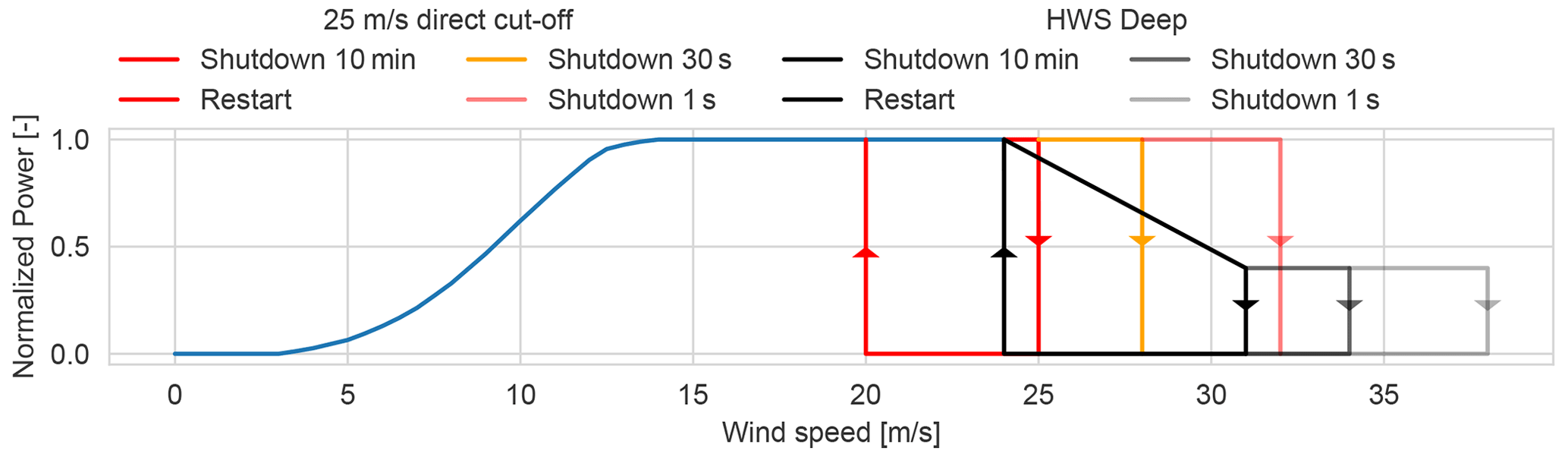
Wind turbine storm shutdown operation consists in four different wind speed set points that specify the mean wind speed shutdown limits for 10 min, 30 s, and 1 s windows (u600, u30, and u1). The turbine goes into shutdown if the wind speed moving average on a period is larger than its limit, for periods of 600, 30, and 1 s. The turbine only goes back into operation when the 10 min moving-average wind speed is lower than the restart wind speed. In the present work modern-turbine high-wind-speed operation (HWS Deep) is modeled with a linear decrease in power and different shutdown wind speed set points. Figure 4 shows the single-turbine storm shutdown for the 25 m s−1 direct cut-off and the HWS Deep technologies.
Wind farm storm shutdown behavior is different from the individual turbine shutdown: in a wind farm not all the turbines will shutdown at exactly the same time because the wind speed fluctuations in each turbine are different, which means that each turbine has a different wind speed time series that reaches shutdown at different times. Macdonald et al. (2014) study the high-wind-speed shutdown behavior of two wind farms in Great Britain. Plant shutdown is characterized by discrete levels of reduced-capacity operation, with each level representing the power curve for the plant when a number of turbines are off. The wind farm storm shutdown hysteresis model presented in Litong-Palima et al. (2016) is extended to model the plant-level operation of turbines with modern high-wind-speed operation. The hysteresis model consists of a simple algorithm that forces the power to move proportionally along the power curve unless the wind speed reaches the restart or shutdown curves; see Fig. 4. The turbine-level storm shutdown is thus first transformed to plant-level behavior based on simulating a set of storm cases in high resolution at a turbine-level generic plant.
CorRES allows the modeling of a wind power plant with both multiple turbines and at the plant level. However, the large-scale simulations of the entire fleet are computationally feasible only at the plant level. Plant simulations with individual turbine storm shutdown simulations are carried out for 15 historical high-wind-speed days (in which max wind speed is larger than 20 m s−1 in the WRF data) at 1 s resolution. These simulations are used to define the plant power curve, the restart line, and the shutdown line; see Fig. 5. In Fig. 5 it can be observed that the high-wind-speed operation part of the plant power curve differs from the piecewise linear behavior of the individual turbine, which is a consequence of the difference between the wind speed fluctuations for each turbine.
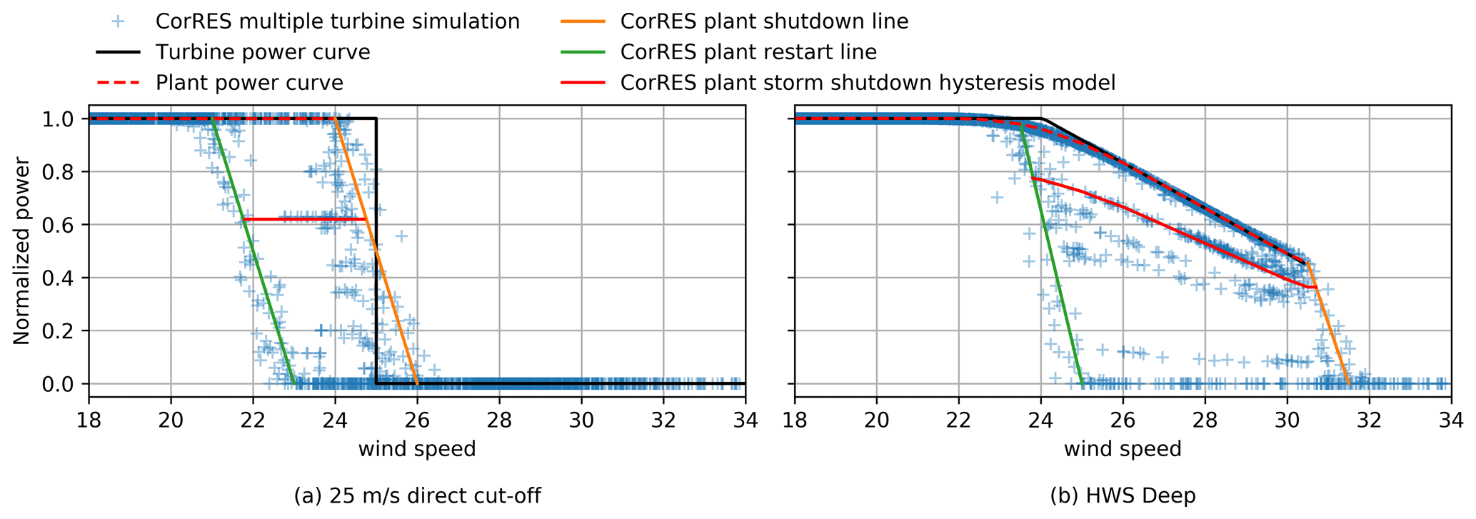
Figure 5Plant vs. single-turbine storm shutdown for (a) 25 m s−1 direct cut-off (b) HWS Deep. Multiple turbine simulations are aggregated in 5 min. The shutdown hysteresis curve (in red) is an example case where restart occurs before the entire plant has shutdown.
3.3 Measured data for model validation and calibration
A total of 4 years of measured generation at 15 min resolution from 2015 to 2018 from the plants in BE2018 are used for model validation; see Fig. 3. Measured generation at 1 min resolution for 2018 is aggregated to 5 min resolution to validate the simulated 5 min ramps. The measured values with wind speed between 5 and 15 m s−1 and no power generation are classified as not available. Such data points were considered to be either measurement errors or an indication that the whole fleet is unavailable.
Wind speed nacelle anemometer measurements are available for the plants in BE2018 at 10 min resolutions from four turbines in the corners of each plant. For comparison to CorRES simulations, the mean of the four turbines is taken to represent the effective wind speed of the plant, and a fleet-level wind speed is defined by taking the weighted mean by installed capacity.
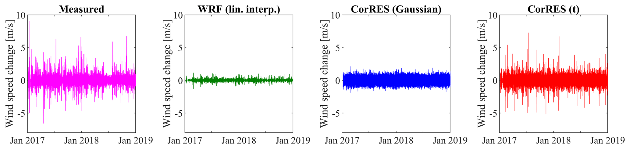
Figure 6Wind speed fluctuations in 10 min: measured, WRF, WRF with Gaussian fluctuations (CorRES(Gaussian)), and WRF with Student t Gaussian copula fluctuations (CorRES(t)).
The wake model wake expansion parameter is calibrated in order to minimize the errors in predicting the capacity factors in the plants of BE2018 during the 2015–2018 period. The wake model calibration produces generation time series with consistent wake/blockage losses as observed in the measurements, but the model applies a constant wake expansion over the whole time series.
Model validation consists in comparing the temporal structure of the wind speed and power time series. A detailed comparison is done in terms of wind speed and power production distributions, wind speed and power fluctuation distributions, and spatial correlation of power and power fluctuations.
Figure 6 illustrates the wind speed fluctuation in 10 min measured and modeled with different approaches. This figure illustrates the need for adding fluctuations to the WRF datasets, and in particular, the need for non-Gaussian-distributed fluctuations.
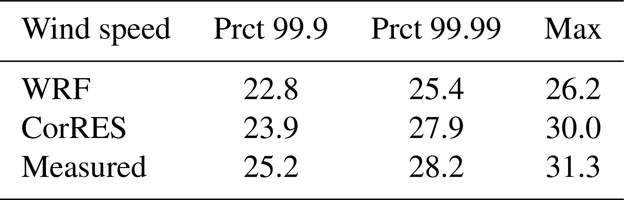
Figure 7 presents the Q–Q plot for the 10 min wind speed fluctuation at each of the plants in BE2018. It can be seen that the introduction of t-distributed fluctuations better represents the measured wind speed fluctuations. Table 2 presents the validation of extreme values of wind speed. It can be seen that WRF without fluctuations and without extreme correction factor (see Eq. 9) underpredicts the extreme wind speeds. The extreme values are better captured by CorRES, but due to the stochastic nature of the fluctuation model, many realizations of the time series will need to be sampled to capture the maxima.
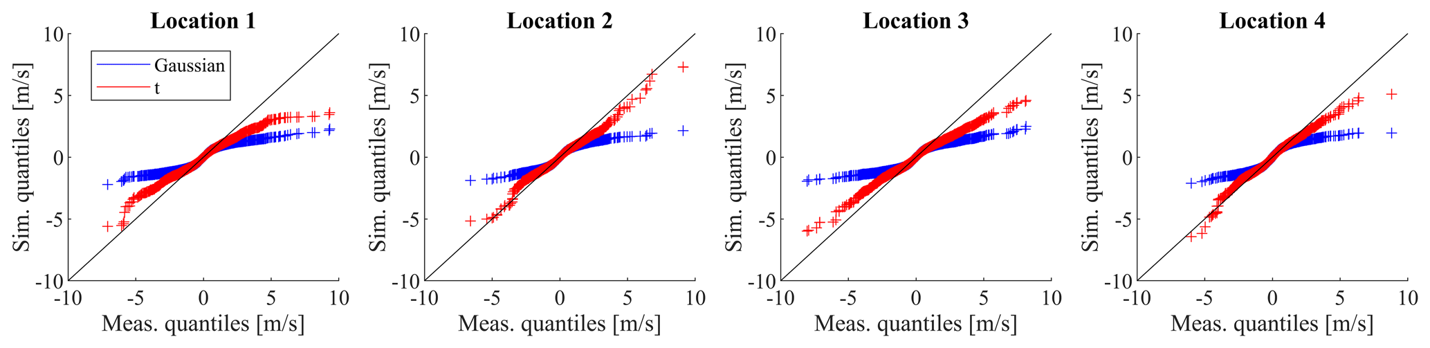
Table 2Extreme (fleet-level mean) wind speed validation by comparing high percentiles (Prct) and maximum.
A comparison of the measured and modeled fleet-level (weighed average of individual plants by installed capacity) wind speed and power distributions of the BE2018 is depicted in Fig. 8. Note that the measured wind speeds include wake deficits (below 14 m s−1), while CorRES wind speed simulations are given without wake losses. CorRES considers the wakes in the plant power curve used to transform wind speed and wind direction to power. Despite this difference, it can be seen that the fleet power production including the storm shutdown is accurately captured. The distribution of power production for measurements and CorRES differs around rated power, because wind turbine availability is not modeled in CorRES.
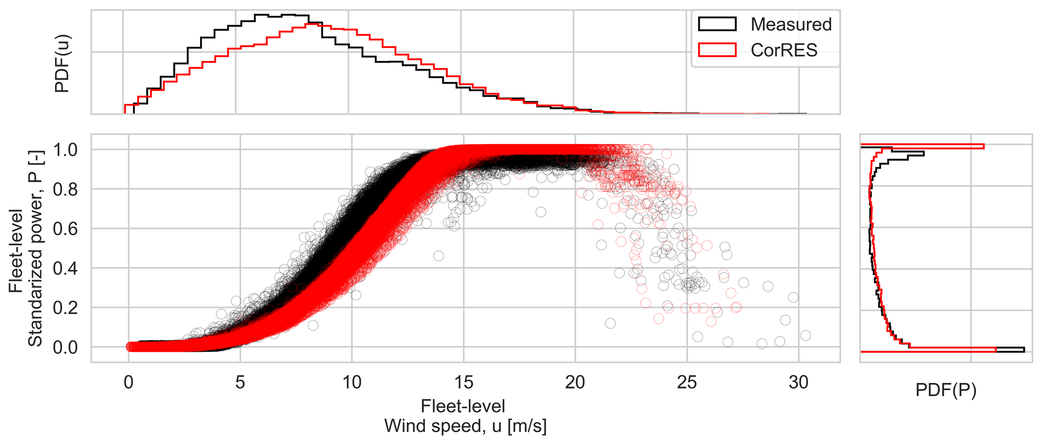
Figure 8Measured and CorRES simulations of power vs. wind speed, with their histograms for BE2018.
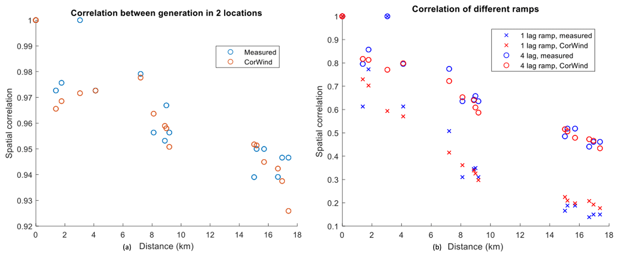
Figure 9(a) Correlation of power production vs. distance between two plants. (b) Correlation of power ramps vs. distance between two plants for 15 min (1 lag) and 60 min (4 lag).
The validation of the spatial correlation of power production and power fluctuations is presented in Fig. 9. Note that CorRES is able to capture the spatial correlation trends: a decrease in correlation between the power of plants as a function of the distance between them. Similarly, the spatial correlation trend for the power ramps (fluctuations) is well reproduced by the simulations. This capability of simulating the spatial and temporal correlation between plants ensures accurate simulations of future-installed-capacity scenarios with different geographical installation distributions.
Model validation results in terms of capacity factors (CFs), standard deviation of standardized production (SD), and standard deviation of different power fluctuation in different time windows (5 min: DP5, 15 min: DP15, 1 h: DP60) are presented in Table 3. The measured fleet CF is slightly overpredicted, which becomes 1.13 % when a standard loss factor from un-availability (0.97) is applied. In this paper, availability is not applied as a factor to the full time series in order to be conservative in the number of full-range power fluctuations.
Table 3BE2018 residuals (prediction error) in capacity factor (CF), standard deviation of standardized power (SD), and standard deviation of 5, 15, and 60 min power fluctuations (DP5, DP15, DP60).

Table 4Capacity factors (CFs), standard deviation of standardized power (SD), and standard deviations of power ramps in 5, 15, and 60 min (SD DP5, SD DP15, SD DP60) and their relative ratios with respect to BE2018. All statistics are computed over the 37 years of simulations.
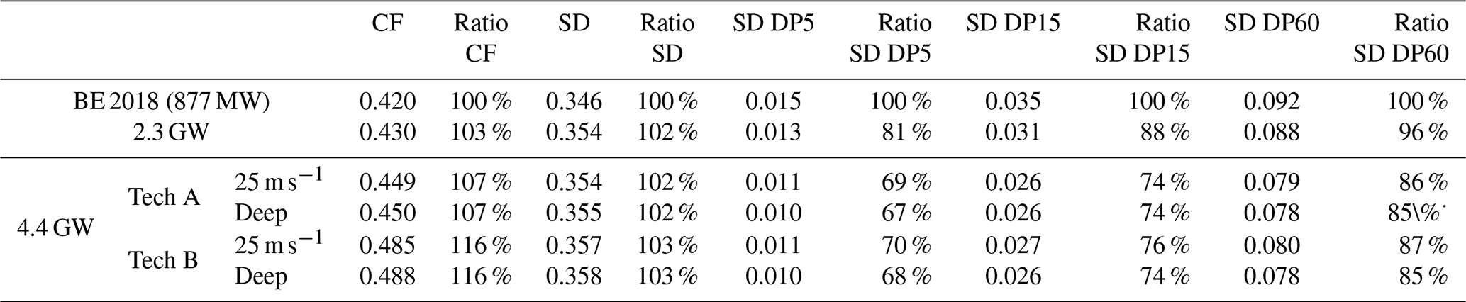
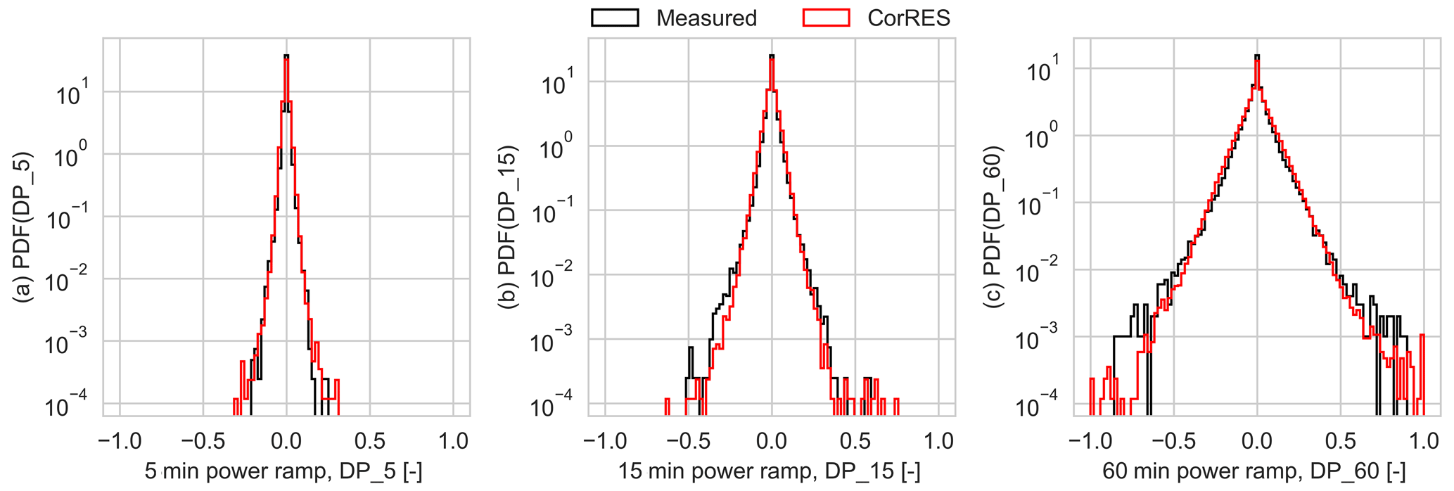
Figure 10Distributions of standardized power fluctuations in different windows: (a) 5 min (DP_5), (b) 15 min (DP_15), and (c) 1 h (DP_60).
The distributions of different power fluctuation in different time windows (5 min, 15 min, 1 h) are presented in Fig. 10. Overall, the distribution of the different power ramps is well captured by the model, besides the small differences on the tails. The difference in the tails is a combination of the lack of an availability model in CorRES, the stochastic nature of the wind speed fluctuation models, and the fact that only 3 years of measurements are available.
Simulation results for 37 years of wind speed time series for the different scenarios (installed capacity, turbine technology, and shutdown technology) in terms of CF, SD, and standard deviation of power ramps (SD DP) are shown in Table 4. The capacity factor of the Belgian offshore wind fleet is expected to increase sequentially from BE2018 to 2.3 GW to the 4.4 GW fleet, due to the use of modern turbines with higher hub heights. A larger capacity factor is obtained when the Tech B is used in the 4.4 GW fleet, while the deep storm shutdown technology only increases the CF marginally.
The standard deviation of the power shows an increase from the BE2018 to BE 2.3 GW scenarios due to the increased capacity factor, installed capacity, hub heights, and larger wake losses. In the 4.4 GW scenario, Tech B shows a slightly larger SD than Tech A due to the steeper power curve and larger hub heights; Tech A does not increase SD with respect to the 2.3 GW scenario.

Figure 11Distributions of standardized power fluctuations during low wind speeds in all the scenarios in different time windows: (a) 5 min (DP_5), (b) 15 min (DP_15), and (c) 1 h (DP_60). The curves for the BE 4.4 GW Tech B scenarios are on top of each other, with only a small difference in the left figure at around DP_5 = 0.2. Tech A is omitted for clarity because it behaves very similar to Tech B.
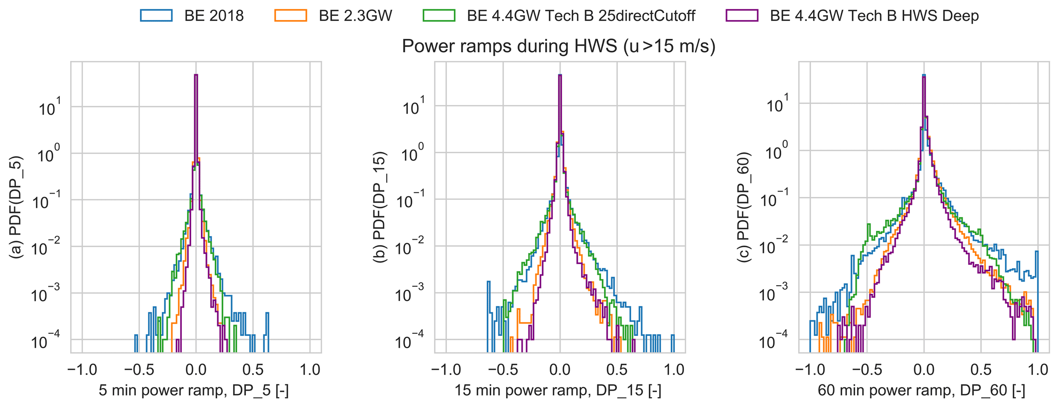
Figure 12Distributions of standardized power fluctuations during high wind speeds in all the scenarios in different time windows: (a) 5 min (DP_5), (b) 15 min (DP_15), and (c) 1 h (DP_60).
The standard deviation of power ramps decreases from BE2018 to 2.3 GW to 4.4 GW, due to the effect of geographical smoothing. There is no significant difference between the standard deviation of the power ramps among turbine or storm shutdown technologies.
Figure 11 presents the comparison of the power fluctuations during low wind speeds (fleet-level weighted-mean wind speed below 15 m s−1) over the different installation/technology scenarios. The 4.4 GW scenarios show the lowest variability of power fluctuations, followed by BE 2.3 GW and BE2018. These fluctuations are mainly caused by wind speed fluctuations and depend on the steepness of the power curve. The distribution of low-wind-speed ramps is symmetric because the power curve behaves almost linearly in this wind speed range.
Similarly, Fig. 12 shows the comparison of the power fluctuations during high wind speeds (fleet-level weighted-mean wind speed larger than 15 m s−1). The geographical smoothing and the high-wind-speed operation significantly reduce the tails (i.e., extreme events) of the power fluctuation distributions. The 2.3 GW scenario shows a large reduction in the extreme power ramping with respect to BE2018 because of the use of HWS storm protection technologies. Furthermore, all scenarios show non-symmetric distributions with larger extreme positive ramps. Extreme negative ramps (at high wind speed) occur when the fleet shuts down during a storm, while large positive ramps occur when the turbines restart after a shutdown during high wind speeds. In the 4.4 GW scenario, the 25 m s−1 direct cut-off shutdown shows the largest extreme power fluctuations for positive and negative ramps at high wind speed with a frequency of mid-range ramp events above the BE 2018 scenario, while BE 4.4 GW HWS Deep shows the least extreme power fluctuations of all scenarios. The extreme positive ramps at high wind speeds for BE 4.4 GW HWS Deep and BE 2.3 GW are larger than the extreme negative ramps; these extreme positive ramps are a consequence of the turbine restart operation.
Table 5Extreme power ramps in 5, 15, and 60 min and their relative ratios with respect to BE2018.

The extreme ramping events during low wind speeds are lower than the ramps at high wind speed for BE2028 and BE 4.4 GW with a 25 m s−1 direct cut-off. Meanwhile, the 2.3 GW and 4.4 GW with HWS Deep scenarios show similar negative extreme power ramp values for low and high wind speeds.
The extreme power ramps in different time windows for all scenarios (at all wind speeds) are summarized in Table 5. There is a reduction in extreme ramps between the BE2018 and 2.3 GW scenarios. In the 4.4 GW scenario, the HWS Deep mitigates the extreme ramp events with respect to both BE2018 and 2.3 GW scenarios, while the reference direct cut-off shows an increase in extreme events. From Table 4 it can be concluded that geographical distribution of installations has a major impact on the general level of variability (standard deviation of power ramps), while Tables 4 and 5 show that the storm shutdown type only impacts the tails of the ramp distribution, especially for DP5 and DP15.
The increase in CF in the 4.4 GW scenario with wind turbine Tech B is due to the larger rotor size and taller hub heights, but financial analysis may result in selections of turbines with less expensive rotors. Similarly, the 2.3 GW scenario showed a larger CF than BE2018 because of the overall trend in increasing rotor sizes and taller tower; see Table 1. This occurs even though there is an increase in wake losses due to the farm-to-farm interaction in BE 2.3 GW; see Fig. 3.
In general, the power fluctuation decreases in the 4.4 GW scenario. This is caused by the larger distances between plants, which cause a geographical smoothing due to lower correlation between the individual plant power time series. These results are consistent with the literature (Holttinen et al., 2016; Koivisto et al., 2016, 2019b, 2020).
There is a trend that shows the most extreme power fluctuations occurring during high wind, such that it is possible to lose 75 % of the installed capacity in 1 h during an extreme storm event. But the use of modern high-wind-speed operation technologies mitigates the impact of extreme ramp-downs to the point that similar extreme ramp-down events are seen at low and high wind speeds. Extreme ramp-ups are more likely to occur than similarly sized ramp-downs, because the wind turbine storm shutdown technologies only mitigate the shutdowns and not the restart part of the power curve. Mitigation of such ramp-up events (during and after storms) should be addressed as they represent some of the largest power fluctuation events.
The extreme ramping events at low wind speeds become equally important as the high-wind-speed extreme ramps when turbines with modern high-wind-speed operation are installed. This means that mitigation approaches that operate at both high and low wind speeds are needed to further reduce power fluctuations. Geographical location of installations has a major impact on the standard deviation of power ramps, and therefore it can be used for further mitigation of power fluctuations.
Even though the t-distribution wind speed fluctuations were deemed necessary to accurately capture the power fluctuations, a more theoretically sound modeling approach could consist in a stochastic model with non-stationary Gaussian wind speed fluctuations, in which the variance is a function of the stability and turbulence intensity time series. These additional variables are available in some of the weather models.
Improved wake modeling could also be implemented in the presented approach. The use of computational fluid dynamics Reynolds-averaged Navier–Stokes (RANS) wake models such as van der Laan et al. (2015) has been proven to be more accurate to predict not only wake losses but also losses due to blockage effects (Bleeg et al., 2018) and therefore produce more accurate generation time series. Due to the large size of the Belgian–Dutch fleet, such simulations were not possible in the present study. Another possible improvement of the wake modeling is to consider stability-dependent plant power curves, which means that the power time series will be interpolated using the wind speed, wind direction, and stability time series. Additional improvements in the inclusion of wind turbine dynamics could create the possibility of making simulations at higher time resolution, but such models were considered out of the scope of this study.
To further reduce the conservatism of the present analysis, a stochastic availability model should be developed. This will remove the discrepancy between the distribution of fleet-level wind power production seen around rated power. Nevertheless, the proposed methodology successfully represented the fleet-level ramp distributions compared with the measured data.
The model validation shows that the methodology presented in this paper is able to capture the distribution of fleet-level wind speed and power production, while at the same time capturing the main spatiotemporal characteristics of the time series. The Student t and extreme wind speed corrections improved the accuracy of simulated extreme events in the wind speed and power fluctuation distributions. The hysteresis plant storm shutdown model is able to capture the modern high-wind-speed operation technologies offered by the main turbine manufacturers. The use of a long time series (37 years) of generation is fundamental in order to quantify the likelihood of the extreme fleet-level power fluctuations.
The future 4.4 GW fleet has an increased capacity factor while at the same time showing a reduction in the standardized power fluctuations with respect to the 2.3 GW fleet. However, for the high-wind-speed events, a reduction of the extreme power ramps is only achievable with the use of modern high-wind-speed operation. Turbines with high-wind-speed operation affect the business case of a project by a marginal increase in the CF and a reduction of the imbalance costs, while at the same time this type of extended range operation makes the turbines more expensive. This means that the imbalance prices should be set to give a financial incentive to the developers to select such technologies. On the energy system level, these technologies are crucial for extreme ramp event mitigation in cases where there is a tightly packed wind power fleet. The most extreme power fluctuations occur in the ramp-up, i.e., in the restart after shutdown, which can be mitigated by controlling the restart. This could be implemented at the turbine level by implementing a gradual restart curve or at the system level by forcing the plants to come back to power in a gradual manner.
The extreme ramping events at low wind speeds become equally important as at high wind speeds when modern high-wind-speed operation is installed in the fleet. This means that approaches that operate at both high and low wind speeds are needed to achieve further reductions of power fluctuations. Geographical distribution of installations has a major impact on reducing the standard deviation of power ramps; therefore plant-to-plant distance should be considered to further mitigate power fluctuations.
The methodology and analysis presented in this paper are relevant for the future offshore installations in the North Sea. It is expected that countries like Germany and the United Kingdom will reach density of offshore installation similar to that currently in Belgium (Agora Energiewende et al., 2020).
The data and code presented in this paper are not publicly available.
JPML and MJK are responsible for writing the article, model development, simulations, and analysis. PS and PM are responsible for supervision and comments.
The authors declare that they have no conflict of interest.
The authors would like to thank the wind plant operators and Elia for providing the validation data.
This research has been supported by the EUDP/ForskEL program (project OffshoreWake. PSO-12521) and the DTU Wind Energy (project La Cour Fellowship – PSfuture).
This paper was edited by Ola Carlson and reviewed by Nermina Saracevic and one anonymous referee.
Agora Energiewende, Agora Verkehrswende, Technical University of Denmark, and Max-Planck-Institute for Biogeochemistry: Making the Most of Offshore Wind: Re-Evaluating the Potential of Offshore Wind in the German North Sea, Tech. rep., available at: https://static.agora-energiewende.de/fileadmin/Projekte/2019/Offshore_Potentials/176_A-EW_A-VW_Offshore-Potentials_Publication_WEB.pdf, last access: 19 March 2020. a, b
Apt, J.: The spectrum of power from wind turbines, J. Power Sour., 169, 369–374, 2007. a
Bastankhah, M. and Porté-Agel, F.: A new analytical model for wind-turbine wakes, Renew. Energy, 70, 116–123, 2014. a
Bastine, D., Larsén, X., Witha, B., Dörenkämper, M., and Gottschall, J.: Extreme winds in the New European Wind Atlas, J. Phys.: Conf. Ser., 1102, 012006, https://doi.org/10.1088/1742-6596/1102/1/012006, 2018. a
Bleeg, J., Purcell, M., Ruisi, R., and Traiger, E.: Wind farm blockage and the consequences of neglecting its impact on energy production, Energies, 11, 1609, https://doi.org/10.3390/en11061609, 2018. a
Buijs, P., Bekaert, D., Van Hertem, D., and Belmans, R.: Needed investments in the power system to bring wind energy to shore in Belgium, in: 2009 IEEE Bucharest PowerTech, 28 June–2 July 2009, Bucharest, Romania, 1–6, 2009. a
Danish Energy Agency: Technology Catalogue, 2020, Tech. rep., available at: https://ens.dk/en/our-services/projections-and-models/technology-data/technology-data-generation-electricity-and, last access: 19 March 2020. a
Dee, D. P., Uppala, S. M., Simmons, A., Berrisford, P., Poli, P., Kobayashi, S., Andrae, U., Balmaseda, M., Balsamo, G., Bauer, P., Bechtold, P., Beljaars, A. C. M., van de Berg, L., Bidlot, J., Bormann, N., Delsol, C., Dragani, R., Fuentes, M., Geer, A. J., Haimberger, L., Healy, S. B., Hersbach, H., Hólm, E. V., Isaksen, L., Kållberg, P., Köhler, M., Matricardi, M., McNally, A. P., Monge-Sanz, B. M., Morcrette, J.-J., Park, B.-K., Peubey, C., de Rosnay, P., Tavolato, C., Thépaut, J.-N., and Vitart, F.: The ERA-Interim reanalysis: Configuration and performance of the data assimilation system, Q. J. Roy. Meteorol. Soc., 137, 553–597, 2011. a, b
Ekström, J., Koivisto, M., Mellin, I., Millar, R. J., and Lehtonen, M.: A statistical model for hourly large-scale wind and photovoltaic generation in new locations, IEEE T. Sustain. Energ., 8, 1383–1393, 2017. a
Elia, B. T. S. O.: Electricity Scenarios for Belgium towards 2050, available at: https://www.elia.be/en/publications/studies-and-reports (last access: 4 June 2020), 2017. a
Elia, B. T. S. O.: Offshore Integration Study, Tech. rep., available at: https://www.elia.be/en/publications/studies-and-reports (last access: 4 June 2020), 2018. a
Elia, B. T. S. O.: Adequacy and flexibility study for Belgium 2020–2030, Tech. rep., available at: https://www.elia.be/en/electricity-market-and-system/document-library (last access: 4 June 2020), 2019. a
Engeland, K., Borga, M., Creutin, J.-D., François, B., Ramos, M.-H., and Vidal, J.-P.: Space-time variability of climate variables and intermittent renewable electricity production – A review, Renew. Sustain. Energ. Rev., 79, 600–617, 2017. a
Fertig, E.: Simulating subhourly variability of wind power output, Wind Energy, 22, 1275–1287, 2019. a
Gelaro, R., McCarty, W., Suárez, M. J., Todling, R., Molod, A., Takacs, L., Randles, C. A., Darmenov, A., Bosilovich, M. G., Reichle, R., Wargan, K., Coy, L., Cullather, R., Draper, C., Akella, S., Buchard, V., Conaty, A., da Silva, A. M., Gu, W., Kim, G.-K., Koster, R., Lucchesi, R., Merkova, D., Nielsen, J. E., Partyka, G., Pawson, S., Putman, W., Rienecker, M., Schubert, S. D., Sienkiewicz, M., and Zhao, B.: The modern-era retrospective analysis for research and applications, version 2 (MERRA-2), J. Climate, 30, 5419–5454, 2017. a
González-Aparicio, I., Monforti, F., Volker, P., Zucker, A., Careri, F., Huld, T., and Badger, J.: Simulating European wind power generation applying statistical downscaling to reanalysis data, Appl. Energy, 199, 155–168, 2017. a, b
Hersbach, H., Bell, B., Berrisford, P., Hirahara, S., Horányi, A., Muñoz-Sabater, J., Nicolas, J., Peubey, C., Radu, R., Schepers, D., Simmons, A., Soci, C., Abdalla, S., Abellan, X., Balsamo, G., Bechtold, P., Biavati, G., Bidlot, J., Bonavita, M., De Chiara, G., Dahlgren, P., Dee, D., Diamantakis, M., Dragani, R., Flemming, J., Forbes, R., Fuentes, M., Geer, A., Haimberger, L., Healy, S., Hogan, R. J., Hólm, E., Janisková, M., Keeley, S., Laloyaux, P., Lopez, P., Lupu, C., Radnoti, G., de Rosnay, P., Rozum, I., Vamborg, F., Villaume, S., and Thépaut, J.-N.: The ERA5 global reanalysis, Q. J. Roy. Meteorol. Soc., 146, 1999–2049, 2020. a
Holttinen, H., Meibom, P., Orths, A., Lange, B., O'Malley, M., Tande, J. O., Estanqueiro, A., Gomez, E., Söder, L., Strbac, G., Smith, J. C., and van Hulle, F.: Impacts of large amounts of wind power on design and operation of power systems, results of IEA collaboration, Wind Energy, 14, 179–192, 2011. a
Holttinen, H., Kiviluoma, J., Forcione, A., Milligan, M., Smith, C. J., Dillon, J., Dobschinski, J., van Roon, S., Cutululis, N., Orths, A., Eriksen, P. B., Carlini, E. M., Estanqueiro, A., Bessa, R., Söder, L., Farahmand, H., Torres, J. R., Jianhua, B., Kondoh, J., Pineda, I., and Strbac, G.: Design and operation of power systems with large amounts of wind power: state of the art report, IEA, available at: https://community.ieawind.org/HigherLogic/System/DownloadDocumentFile.ashx?DocumentFileKey=87ada8ed-5a95-20bd-2bd8-5174e6e065d6 & forceDialog=0 (last access: 4 June 2020), 2016. a, b, c
Huber, M., Dimkova, D., and Hamacher, T.: Integration of wind and solar power in Europe: Assessment of flexibility requirements, Energy, 69, 236–246, 2014. a
Kiviluoma, J., Holttinen, H., Weir, D., Scharff, R., Söder, L., Menemenlis, N., Cutululis, N. A., Danti Lopez, I., Lannoye, E., Estanqueiro, A., Gomez-Lazaro, E., Zhang, Q., Bai, J., Wan, Y.-H., and Milligan, M.: Variability in large-scale wind power generation, Wind Energy, 19, 1649–1665, 2016. a
Klöckl, B. and Papaefthymiou, G.: Multivariate time series models for studies on stochastic generators in power systems, Elect. Power Syst. Res., 80, 265–276, 2010. a
Koivisto, M., Ekström, J., Seppänen, J., Mellin, I., Millar, J., and Haarla, L.: A statistical model for comparing future wind power scenarios with varying geographical distribution of installed generation capacity, Wind Energy, 19, 665–679, 2016. a, b, c, d
Koivisto, M., Das, K., Guo, F., Sørensen, P., Nuño, E., Cutululis, N., and Maule, P.: Using time series simulation tools for assessing the effects of variable renewable energy generation on power and energy systems, Wiley Interdisciplin. Rev.: Energ. Environ., 8, e329, https://doi.org/10.1002/wene.329, 2019a. a
Koivisto, M., Maule, P., Cutululis, N., and Sørensen, P.: Effects of Wind Power Technology Development on Large-scale VRE Generation Variability, in: 2019 IEEE Milan PowerTech, 23–27 June 2019, Milan, Italy, 1–6, 2019b. a, b
Koivisto, M., Jónsdóttir, G. M., Sørensen, P., Plakas, K., and Cutululis, N.: Combination of meteorological reanalysis data and stochastic simulation for modelling wind generation variability, Renew. Energy, 159, 991–999, https://doi.org/10.1016/j.renene.2020.06.033, 2020. a, b, c, d, e
Larsén, X. G. and Kruger, A.: Application of the spectral correction method to reanalysis data in South Africa, J. Wind Eng. Indust. Aerodynam., 133, 110–122, 2014. a
Larsén, X. G., Ott, S., Badger, J., Hahmann, A. N., and Mann, J.: Recipes for correcting the impact of effective mesoscale resolution on the estimation of extreme winds, J. Appl. Meteorol. Clim., 51, 521–533, 2012. a
Larsén, X. G., Larsen, S. E., and Petersen, E. L.: Full-scale spectrum of boundary-layer winds, Bound.-Lay. Meteorol., 159, 349–371, 2016. a
Leahy, P. G. and Foley, A. M.: Wind generation output during cold weather-driven electricity demand peaks in Ireland, Energy, 39, 48–53, 2012. a
Litong-Palima, M., Bjerge, M. H., Cutululis, N. A., Hansen, L. H., and Sørensen, P.: Modeling of the dynamics of wind to power conversion including high wind speed behavior, Wind Energy, 19, 923–938, 2016. a, b
Liu, H., Jin, Y., Tobin, N., and Chamorro, L. P.: Towards uncovering the structure of power fluctuations of wind farms, Phys. Rev. E, 96, 063117, https://doi.org/10.1103/PhysRevE.96.063117, 2017. a
Liu, Y., Warner, T., Liu, Y., Vincent, C., Wu, W., Mahoney, B., Swerdlin, S., Parks, K., and Boehnert, J.: Simultaneous nested modeling from the synoptic scale to the LES scale for wind energy applications, J. Wind Eng. Indust. Aerodynam., 99, 308–319, 2011. a, b
Macdonald, H., Hawker, G., and Bell, K.: Analysis of wide-area availability of wind generators during storm events, in: 2014 International Conference on Probabilistic Methods Applied to Power Systems (PMAPS), 7–10 July 2014, Durham, UK, 1–6, 2014. a
Marinelli, M., Maule, P., Hahmann, A. N., Gehrke, O., Nørgrd, P. B., and Cutululis, N. A.: Wind and photovoltaic large-scale regional models for hourly production evaluation, IEEE T. Sustain. Energ., 6, 916–923, 2014. a
Mehrens, A. R., Hahmann, A. N., Larsén, X. G., and von Bremen, L.: Correlation and coherence of mesoscale wind speeds over the sea, Q. J. Roy. Meteorol. Soc., 142, 3186–3194, 2016. a, b
Mikova, N., Eichhammer, W., and Pfluger, B.: Low-carbon energy scenarios 2050 in north-west European countries: Towards a more harmonised approach to achieve the EU targets, Energy Policy, 130, 448–460, 2019. a
Nuño, E., Maule, P., Hahmann, A., Cutululis, N., Sørensen, P., and Karagali, I.: Simulation of transcontinental wind and solar PV generation time series, Renew. Energy, 118, 425–436, 2018. a, b
Olauson, J.: ERA5: The new champion of wind power modelling?, Renew. Energy, 126, 322–331, 2018. a
Olauson, J. and Bergkvist, M.: Modelling the Swedish wind power production using MERRA reanalysis data, Renew. Energy, 76, 717–725, https://doi.org/10.1016/j.renene.2014.11.085, 2015. a
Olauson, J., Bergström, H., and Bergkvist, M.: Restoring the missing high-frequency fluctuations in a wind power model based on reanalysis data, Renew. Energy, 96, 784–791, 2016. a
Olauson, J., Bergkvist, M., and Rydén, J.: Simulating intra-hourly wind power fluctuations on a power system level, Wind Energy, 20, 973–985, 2017. a
Pfenninger, S.: Dealing with multiple decades of hourly wind and PV time series in energy models: A comparison of methods to reduce time resolution and the planning implications of inter-annual variability, Appl. Energy, 197, 1–13, 2017. a, b
Pfenninger, S., Hawkes, A., and Keirstead, J.: Energy systems modeling for twenty-first century energy challenges, Renew. Sustain. Energ. Rev., 33, 74–86, 2014. a
Porté-Agel, F., Bastankhah, M., and Shamsoddin, S.: Wind-turbine and wind-farm flows: a review, Bound.-Lay. Meteorol., 174, 1–59, 2020. a, b, c
Roques, F., Hiroux, C., and Saguan, M.: Optimal wind power deployment in Europe – A portfolio approach, Energy Policy, 38, 3245–3256, 2010. a
Santos-Alamillos, F., Thomaidis, N., Usaola-García, J., Ruiz-Arias, J., and Pozo-Vázquez, D.: Exploring the mean-variance portfolio optimization approach for planning wind repowering actions in Spain, Renew. Energy, 106, 335–342, 2017. a
Skamarock, W. C., Klemp, J. B., Dudhia, J., Gill, D. O., Barker, D. M., Wang, W., and Powers, J. G.: A description of the Advanced Research WRF version 3, NCAR Technical note-475+ STR, University Corporation for Atmospheric Research, https://doi.org/10.5065/D68S4MVH, 2008. a, b
Sørensen, P., Hansen, A. D., and Rosas, P. A. C.: Wind models for simulation of power fluctuations from wind farms, J. Wind Eng. Indust. Aerodynam., 90, 1381–1402, 2002. a
Sørensen, P., Cutululis, N. A., Vigueras-Rodríguez, A., Madsen, H., Pinson, P., Jensen, L. E., Hjerrild, J., and Donovan, M.: Modelling of power fluctuations from large offshore wind farms, Wind Energy, 11, 29–43, 2008. a, b
Sørensen, P., Litong-Palima, M., Hahmann, A. N., Heunis, S., Ntusi, M., and Hansen, J. C.: Wind power variability and power system reserves in South Africa, J. Energ. South. Africa, 29, 59–71, 2018. a
Sørensen, P., Koivisto, M., and Murcia, J.: Elia – MOG II System Integration: Public version, no. E-0203 in DTU Wind Energy E, DTU Wind Energy, Denmark, 2020. a
Staffell, I. and Pfenninger, S.: Using bias-corrected reanalysis to simulate current and future wind power output, Energy, 114, 1224–1239, 2016. a
Staffell, I. and Pfenninger, S.: The increasing impact of weather on electricity supply and demand, Energy, 145, 65–78, 2018. a
Talbot, C., Bou-Zeid, E., and Smith, J.: Nested mesoscale large-eddy simulations with WRF: Performance in real test cases, J. Hydrometeorol., 13, 1421–1441, 2012. a, b
Tejeda, C., Gallardo, C., Domínguez, M., Gaertner, M. Á., Gutierrez, C., and de Castro, M.: Using wind velocity estimated from a reanalysis to minimize the variability of aggregated wind farm production over Europe, Wind Energy, 21, 174–183, 2018. a
Thomaidis, N. S., Santos-Alamillos, F. J., Pozo-Vázquez, D., and Usaola-García, J.: Optimal management of wind and solar energy resources, Comput. Operat. Res., 66, 284–291, 2016. a
van der Laan, M. P., Sørensen, N. N., Réthoré, P.-E., Mann, J., Kelly, M. C., Troldborg, N., Hansen, K. S., and Murcia, J. P.: The κ–ϵ–fP model applied to wind farms, Wind Energy, 18, 2065–2084, 2015. a
Veers, P. S.: Three-dimensional wind simulation, Tech. rep., Sandia National Labs., Albuquerque, NM, USA, 1988. a, b
Volker, P. J., Hahmann, A. N., Badger, J., and Jørgensen, H. E.: Prospects for generating electricity by large onshore and offshore wind farms, Environ. Res. Lett., 12, 034022, https://doi.org/10.1088/1748-9326/aa5d86, 2017. a, b
Von Bremen, L.: Large-scale variability of weather dependent renewable energy sources, in: Management of weather and climate risk in the energy industry, edited by: Troccoli, A., Springer Netherlands, Dordrecht, 189–206, ISBN 978-90-481-3692-6, 2010. a