Optimal scheduling of the next preventive maintenance activity for a wind farm

A large part of the operational cost for a wind farm is due to the cost of equipment maintenance, especially for offshore wind farms. How to reduce the maintenance cost, and hence increase profitability, is this article's focus. It presents a binary linear optimization model whose solution may inform the wind turbine owners about which components, and when, should undergo the next preventive maintenance (PM) replacements. The suggested short-term scheduling strategy takes into account eventual failure events of the multi-component system – in that after the failed system is repaired, the previously scheduled PM plan should be updated, assuming that the restored components are as good as new.

The optimization algorithm of this paper, NextPM, is tested through numerical case studies applied to a four-component model of a wind turbine. The first study addresses the important case of a single component system, used for parameter calibration purposes. The second study analyses the case of seasonal variations of mobilization costs, as compared to the constant mobilization cost setting. Among other things, this analysis reveals a 35 % cost reduction achieved by the NextPM model, as compared to the pure corrective maintenance (CM) strategy. The third case study compares the NextPM model with another optimization model – the preventive maintenance scheduling problem with interval costs (PMSPIC), which was the major source of inspiration for this article. This comparison demonstrates that the NextPM model is accurate and much faster in terms of computational time.

1 Introduction

Wind energy is one of the lowest-priced renewable energy technologies available today; see Lazard (2020). A large part of the total cost associated with wind turbines is due to operation and maintenance, amounting to 34 % for the fixed-bottom offshore wind turbines, according to Stehly and Beiter (2020). To reduce the maintenance cost, one can improve the design of the components, making them more reliable. One can also reduce the maintenance costs by means of an improved scheduling of the maintenance activities for still-functioning components depending on their current age. The latter task is the main concern of this paper, which proposes an optimization model for preventive maintenance (PM) scheduling of a wind turbine or even a farm of wind turbines. Notice that, in this paper, by PM activities we do not mean the practice of regular inspection of the component's condition. Our concern is the optimal planning of preventive replacements of the components based on their current age.

Typically, a maintenance model distinguishes between a corrective maintenance (CM) event, when a component should be attended after it breaks down, and a PM event, when one or several older components are renewed before they break down, see the recent survey (Lee and Cha, 2016). An optimal PM scheduling is aimed at reducing the lost production due to the downtime caused by CM events.

There is a multitude of papers devoted to the optimal PM scheduling for multi-component systems; see Werbińska-Wojciechowska (2019). The article Jafari et al. (2018) proposes a joint optimization of the maintenance policy and the inspection interval for a multi-unit series system with economic dependence. It develops an algorithm aiming at a maintenance policy for a multi-component system minimizing the maintenance cost, under the assumption that one unit of the system is subject to condition monitoring, while for the other units only the age information is available. Tian et al. (2014) develop a method to quantify the uncertainty of the remaining life length, resulting in an effective condition-based maintenance approach to optimal scheduling.

The article Sarker and Faiz (2016) looks at opportunistic maintenance (OM), which is a special kind of a PM activity occurring at the time of a CM replacement: replacing still-functioning components together with the broken one may save some mobilization costs. OM activities are shown to be extremely beneficial for the offshore wind farms, due to the large mobilization costs.

In Moghaddam and Usher (2011), optimization models are developed to determine the optimal PM schedules in repairable and maintainable systems. They show that if mobilization costs are the same irrespective of the number of components to be attended, then multiple simultaneous PM activities become cost-effective. However, their optimization models are nonlinear and non-convex, which makes them computationally hard to solve; see Sect. 1.3 in Andreasson et al. (2020).

The preventive maintenance scheduling problem with interval costs (PMSPIC) model from Gustavsson et al. (2014) was the major inspiration for this work. The main feature of the PMSPIC model is the idea of interval cost: given a time interval between two consecutive PM activities, the expected maintenance cost should take into account eventual breakdowns of components during this time interval. The PMSPIC model has a long computational time, which motivated us to build a new optimization model for PM scheduling of a wind turbine.

In this paper, we build on the state of the art with a new algorithm, NextPM. Given the current ages of the key components of the system, NextPM computes the best time to perform the next maintenance activity and determines which components should be replaced at that time. The algorithm can be solved in 1 s and thus has a potential for being used as a key module in a maintenance scheduling app for wind turbines.

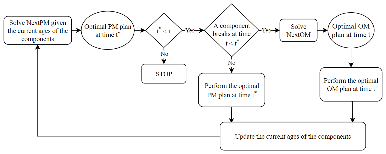
The paper is organized as follows. Section 2 presents a novel optimization model for maintenance scheduling of a multi-component system. In the context of wind farm maintenance, each wind turbine is viewed here as a system comprising multiple components such as the gearbox, power generator, rotor, and main bearing. Whenever one of the components is broken, the whole system stops functioning. After the broken component is replaced by a new one, the system resumes its function. It is assumed that at time 0 all components of the system are new and that the total lifespan of the system is T units of time. The model has a discrete time setting t=0, 1, …, T, where the unit of time can be either a day, a month, or a year, depending on a concrete application; see Browell et al. (2016) for a maintenance scheduling with only 1 d ahead. In the same Sect. 2, the main result of the paper is summarized as Algorithm 1, aiming at an optimal PM schedule for the time period [s, T] with an arbitrary starting time $s\in [\mathrm{0},T-\mathrm{1}]$. Figure 1 gives a non-technical description of the algorithm.

Figure 1 Flow diagram of the optimization algorithm involving NextPM as a major step.

The key ingredient of Algorithm 1, the NextPM optimization model, is carefully described in Sect. 3. Section 4 contains several numerical studies that demonstrate the flexibility of our approach, its accuracy, and computational effectiveness. Finally, Sect. 5 presents the main conclusions of the paper.

2 Optimal rescheduling algorithm

Consider a system composed of n components characterized by different life length distributions. For the component j, it is assumed that its total life length L_j is a random variable having a Weibull distribution with parameters (α_j, β_j), so that the corresponding survival function is

$$\begin{array}{}\text{(1)}& P\left(L_j>t\right)=e^{-{\left(\frac{t}{{\mathit{\alpha }}_j}\right)}^{{\mathit{\beta }}_j}},t\ge \mathrm{0},j=\mathrm{1},\mathrm{\dots },n;\end{array}$$

see Guo et al. (2009) concerning the use of the Weibull distribution for the modeling of multi-component systems. The means and variances of the component life lengths are the following functions of the Weibull parameters:

$$\begin{array}{}\text{(2)}& \begin{array}{rl}{\mathit{\mu }}_j=& {\mathit{\alpha }}_j\mathrm{\Gamma }\left(\mathrm{1}+{\displaystyle \frac{\mathrm{1}}{{\mathit{\beta }}_j}}\right),{\mathit{\sigma }}_j^{\mathrm{2}}={\mathit{\alpha }}_j^{\mathrm{2}}\mathrm{\Gamma }\left(\mathrm{1}+{\displaystyle \frac{\mathrm{2}}{{\mathit{\beta }}_j}}\right)-{\mathit{\mu }}_j^{\mathrm{2}},\\ & j=\mathrm{1},\mathrm{\dots },n.\end{array}\end{array}$$

Besides the Weibull parameters (α_j, β_j), j=1, …, n, our optimization model requires the following parameters associated with various maintenance costs: d_t is the time-dependent mobilization cost for either a PM or CM activity, t=0, …, T, b_j is the CM cost of the component j=1, …, n, and c_j is the PM cost of the component j=1, …, n. The full set of the model parameters {d₁, …, $d_T,({\mathit{\alpha }}_{\mathrm{1}},{\mathit{\beta }}_{\mathrm{1}},b_{\mathrm{1}},c_{\mathrm{1}}),\mathrm{\dots },({\mathit{\alpha }}_n,{\mathit{\beta }}_n,b_n,c_n),\mathit{\lambda }\mathit{\}}$ includes an extra parameter λ introduced in Sect. 3.2 by Eq. (11).

Suppose that the multi-component system is observed at some time $s\in [\mathrm{0},T-\mathrm{1}]$, and the latest maintenance times of components j=1, …, n are known to be $t_j\in [\mathrm{0},s]$, so that at the time s, the n components have the effective ages (s−t₁, …, s−t_n). The NextPM optimization model described in Sect. 3 has the input (t₁, …, t_n, s, r), where $r\in [s+\mathrm{1},T]$ is the end of the current planning period. The output of NextPM is a PM plan specifying the optimal time $\mathit{\tau }\in [s+\mathrm{1},r+\mathrm{1}]$ of the next PM event, as well as the set of components $\mathcal{P}\subset \mathit{\{}\mathrm{1},\mathrm{\dots },n\mathit{\}}$ which should be maintained at the time τ. In particular, the output $\mathit{\tau }=r+\mathrm{1}$ means that no PM activity should be scheduled during the planning period [$s+\mathrm{1},r$], implying that the set 𝒫 is empty.

The NextPM model is the key module of the following Algorithm 1 aiming at the long-term PM scheduling until the end time T, at which the whole system is expected to be dismantled; see Fig. 1 for a flow chart illustrating the major steps of Algorithm 1.

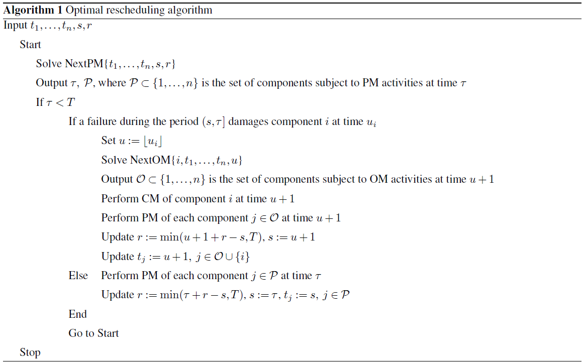
Algorithm 1 relies on a rescheduling procedure, where each NextPM step covering r−s units of the planning time is accompanied by a NextOM module. The latter is a modification of the NextPM step (see Sect. 3.5), which addresses the possibility of a component failure before the planned PM, followed by an OM activity.

3 An optimal plan for the next preventive maintenance

This section sets up the optimization model NextPM, which is the key ingredient of Algorithm 1 summarized in Sect. 2. The optimization model PMSPIC of Gustavsson et al. (2014) was a major motivation for NextPM, and we start by comparing these two approaches using Figs. 2 and 3, which illustrate two different definitions of the objective functions for two optimization models in question.

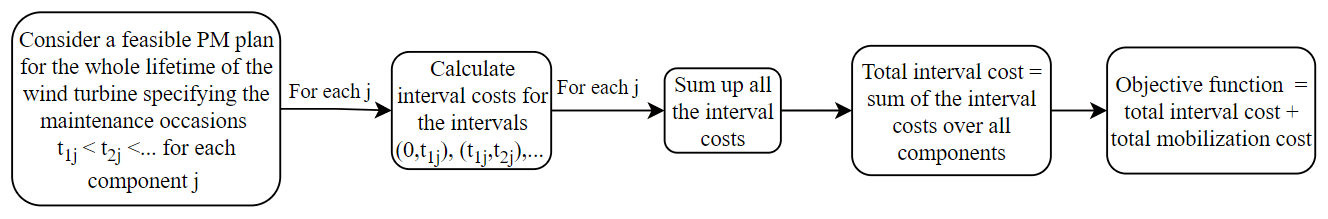
Figure 2 A flow diagram demonstrating how the PMSPIC calculates the objective function for a given feasible maintenance plan.

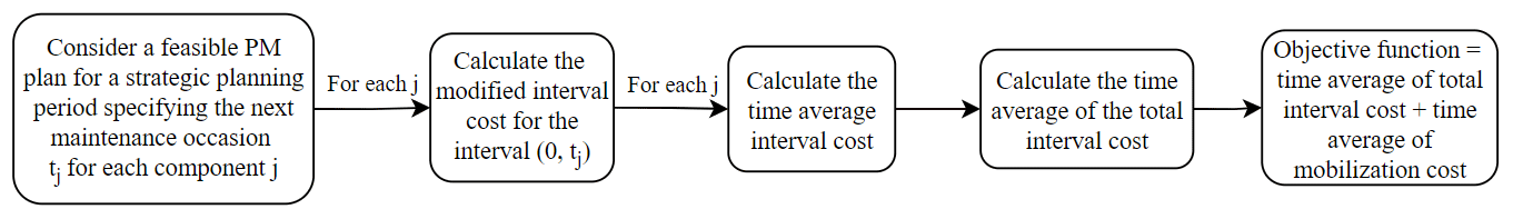
Figure 3 A flow diagram demonstrating how NextPM model calculates the objective function for a given feasible maintenance plan with s=0.

The main difference between PMSPIC and NextPM model is that while PMSPIC generates a maintenance plan for the whole lifetime of the wind turbine, the NextPM model produces an optimal schedule only for the next PM activity. To this end, PMSPIC looks into the total maintenance cost, while NextPM aims at minimizing the time average maintenance cost.

3.1 NextPM model

The purpose of the NextPM model is to produce an optimal PM plan for the period [$s+\mathrm{1},r$], where the planning time span r−s is chosen so that it is reasonable to expect at most one PM event during time r−s. For a given planning period $[s+\mathrm{1},r]\subset [\mathrm{0},T]$, an (s,r) plan is defined as a collection (z, x¹, …, xⁿ) of vectors

$$\begin{array}{ll}{\displaystyle }\mathit{z}=& {\displaystyle }\left(z_{s+\mathrm{1}},\mathrm{\dots },z_{r+\mathrm{1}}\right),{\mathit{x}}^j=\left(x_{s+\mathrm{1}}^j,\mathrm{\dots },x_{r+\mathrm{1}}^j\right),\\ {\displaystyle }& {\displaystyle }j=\mathrm{1},\mathrm{\dots },n,\end{array}$$

with binary coordinates z_t, $x_t^j\in \mathit{\{}\mathrm{0},\mathrm{1}\mathit{\}}$, which satisfy the following linear conditions:

$$\begin{array}{}\text{(3)}& {\displaystyle }& {\displaystyle }\sum _{t=s+\mathrm{1}}^{r+\mathrm{1}}{x}_t^j=\mathrm{1},j=\mathrm{1},\mathrm{\dots },n,\text{(4)}& {\displaystyle }& {\displaystyle }{x}_t^j\le z_t,t=s+\mathrm{1},\mathrm{\dots },r+\mathrm{1},j=\mathrm{1},\mathrm{\dots },n.\end{array}$$

For $t=s+\mathrm{1}$, … r, the equality $x_t^j=\mathrm{1}$ means that according to the (s, r) plan, component j should undergo a PM replacement at time t, provided no component failure during the time period [$s+\mathrm{1},$t]. In contrast, the equality $x_{r+\mathrm{1}}^j=\mathrm{1}$ means that according to the (s, r) plan, no PM activity should involve component j during the time period [$s+\mathrm{1},r$]. On the whole system level, the equality z_t=1 means that according to the (s, r) plan, at least one component should undergo a PM replacement at time t, provided no component failure during the time period [$s+\mathrm{1},t$], and the equality $z_{r+\mathrm{1}}=\mathrm{1}$ means that according to the (s, r) plan, no PM activity is scheduled for the time period [$s+\mathrm{1},r$].

The NextPM optimization model is built around the objective function:

$$\begin{array}{}\text{(5)}& \begin{array}{rl}f\left(\mathit{z},{\mathit{x}}^{\mathrm{1}},\mathrm{\dots },{\mathit{x}}^n\right)& =\sum _{t=s+\mathrm{1}}^{r+\mathrm{1}}{\displaystyle \frac{\mathrm{1}}{t-s}}\left(d_t{z}_t+c_{s,t}^{\mathrm{1}}{x}_t^{\mathrm{1}}\right.\\ & \left.+\mathrm{\dots }+c_{s,t}^n{x}_t^n\right),\end{array}\end{array}$$

where d_tz_t stands for the mobilization cost and the terms $c_{s,t}^j$ are the so-called interval costs defined in Sect. 3.2. The objective function (Eq. 5) can be viewed as the time average maintenance cost per time unit according to the (s, t) plan (z, x¹, …, xⁿ).

Let ($\stackrel{\mathrm{‾}}{\mathit{z}}$, $\stackrel{\mathrm{‾}}{\mathit{x}}$) be the solution to the linear optimization problem

$$\begin{array}{}\text{(6)}& \mathrm{minimize}f\left(\mathit{z},{\mathit{x}}^{\mathrm{1}},\mathrm{\dots },{\mathit{x}}^n\right)\end{array}$$

over all (s, t) plans subject to the linear constraints

$$\begin{array}{}\text{(7)}& D_{s,t}^j{x}_t^j\ge \mathrm{0},t=s+\mathrm{1},\mathrm{\dots },r,j=\mathrm{1},\mathrm{\dots },n,\end{array}$$

where $D_{s,t}^j$ is defined in Sect. 3.3 as the PM benefit for the component j at time t. Then the NextPM algorithm (τ, 𝒩) computes the optimal time of the next PM by

$$\mathit{\tau }={\min }_j\left\{{\mathrm{argmax}}_t{\stackrel{\mathrm{‾}}{x}}_t^j\right\}$$

and determines the set of the components that should undergo the maintenance activities at time τ using

$$\mathcal{N}=\left\{\begin{array}{ll}\left\{j:{\stackrel{\mathrm{‾}}{x}}_{\mathit{\tau }}^j=\mathrm{1},j=\mathrm{1},\mathrm{\dots },n\right\}& \mathrm{if}\mathit{\tau }\le r,\\ \mathrm{\varnothing }& \mathrm{if}\mathit{\tau }=r+\mathrm{1}.\end{array}\right.$$

3.2 Definition of modified interval costs $c_{s,t}^j$

Here we deal with the term $c_{s,t}^j$ appearing in the objective function (Eq. 5) of the optimization model NextPM. The main idea is to define $c_{s,t}^j$ as the fixed PM cost c_j plus the expected additional costs due to eventual failures of the component j occurring prior to the planned PM activity at time t.

To this end, consider n independent sequences of renewal times with a delay by letting $U_{s,\mathrm{0}}^j=s$,

$$\begin{array}{}\text{(8)}& U_{s,\mathrm{1}}^j=t_j+L_{\mathrm{1}j},L_{\mathrm{1}j}\stackrel{d}{=}\left\{L_j|L_j>s-t_j\right\},\end{array}$$

where $\stackrel{d}{=}$ means equality in distribution (conditional distribution in the above formula), and

$$\begin{array}{}\text{(9)}& U_{s,i+\mathrm{1}}^j=U_{s,i}^j+L_{ij},L_{ij}\stackrel{d}{=}{L}_j,\mathrm{for}i=\mathrm{2},\mathrm{3},\mathrm{\dots },\end{array}$$

assuming that the random variables (L_ij) are mutually independent. Notice that in the important particular case s=0, this definition simplifies, so that for each j, the sequence $\mathit{\{}{U}_{\mathrm{0},i}^j{\mathit{\}}}_{i\ge \mathrm{0}}$ describes a renewal process without a delay.

Treating $U_{s,\mathrm{1}}^j$, $U_{s,\mathrm{2}}^j$, … as the sequence of consecutive failure times of the component j, put

$$\begin{array}{}\text{(10)}& c_{s,t}^j:=c_j+E\left(\sum _{i=\mathrm{1}}^{\mathrm{\infty }}{\mathrm{1}}_{\left\{U_{s,i}^j\le t\right\}}{G}_j\left(U_{s,i-\mathrm{1}}^j,L_{ij},t-s\right)\right),\end{array}$$

where the cost functions

$$\begin{array}{}\text{(11)}& \begin{array}{rl}{G}_j(s,u,v)=& b_j+d_{s+u}-{\left({\displaystyle \frac{u}{v}}\right)}^{\mathit{\lambda }}\left(c_j+d_{s+v}\right),\\ & \mathrm{0}\le u\le v,\end{array}\end{array}$$

involve a new parameter λ>0 assumed to be independent of j=1, …, n. The definition of the cost function (Eq. 11) further develops the key idea of Sect. 5.1 in Gustavsson et al. (2014). It describes the additional cost implied by an eventual breakdown of component j before the planned PM activity.

The expression (Eq. 11) is suggested as a compromise between two extreme cases: a failure at the start of the planning period, u=0, and a failure just before the planned PM replacement, $u=v=t-s$. If u is close to 0, then the failure at time s+u will not change the PM plan, implying that the much smaller additional cost

$$\begin{array}{}\text{(12)}& G_j(s,\mathrm{0},t)=b_j+d_s\end{array}$$

is the sum of the CM cost b_j and the mobilization cost d_s at time s. On the other hand, if u is close to $v=t-s$, then the additional cost

$$\begin{array}{}\text{(13)}& G_j(s,t,t-s)=b_j-c_j\end{array}$$

is simply the difference between the CM and PM costs. For $u\in (\mathrm{0},v)$, the expression on the right-hand side of Eq. (11) produces an additional cost which lies between the extreme values (Eqs. 12 and 13). The role of the parameter λ is to control to what extent the proximity of the failure time to the planned PM time influences the extra costs. For example, if λ=1 the intermediate cost is found by a linear extrapolation.

3.3 Definition of $D_{s,t}^j$

The constraint (Eq. 7) arises as a checkup step to ensure that a suggested PM at time t brings some benefit, as compared to a simple strategy when no PM is performed. With the PM-free strategy, the total maintenance cost (including mobilization costs) for the component j during the period [s, T] would be

$$E\left[\sum _{i=\mathrm{1}}^{\mathrm{\infty }}{\mathrm{1}}_{\left\{U_{s,i}^j\le T\right\}}\left(b_j+d_{U_{s,i}^j}\right)\right].$$

Alternatively, if the plan is to perform a PM for the component j at time t, and then to perform replacements of the component j whenever it breaks down, then the total cost would be

$$c_{s,t}^j+E\left[\sum _{i=\mathrm{1}}^{\mathrm{\infty }}{\mathrm{1}}_{\left\{t+U_{\mathrm{0},i}^j\le T\right\}}\left(b_j+d_{t+U_{\mathrm{0},i}^j}\right)\right].$$

Taking into account the difference between these two total costs,

$$\begin{array}{}\text{(14)}& \begin{array}{rl}{D}_{s,t}^j& =E\left[\sum _{i=\mathrm{1}}^{\mathrm{\infty }}{\mathrm{1}}_{\left\{U_{s,i}^j\le T\right\}}\left(b_j+d_{U_{s,i}^j}\right)\right]-c_{s,t}^j\\ & -E\left[\sum _{i=\mathrm{1}}^{\mathrm{\infty }}{\mathrm{1}}_{\left\{t+U_{\mathrm{0},i}^j\le T\right\}}\left(b_j+d_{t+U_{\mathrm{0},i}^j}\right)\right],\end{array}\end{array}$$

we conclude that the planned PM of the component j at time t is justified only if $D_{s,t}^j\ge \mathrm{0}$.

3.4 Complete optimization model of NextPM

Here we put together the complete optimization model of the NextPM step:

$$\begin{array}{ll}{\displaystyle }& {\displaystyle }\mathrm{minimize}f\left(\mathit{z},{\mathit{x}}^{\mathrm{1}},\mathrm{\dots },{\mathit{x}}^n\right):=\sum _{t=s+\mathrm{1}}^{r+\mathrm{1}}{\displaystyle \frac{\mathrm{1}}{t-s}}\left(d_t{z}_t+c_{s,t}^{\mathrm{1}}{x}_t^{\mathrm{1}}\right.\\ {\displaystyle }& {\displaystyle }\left.+\mathrm{\dots }+c_{s,t}^n{x}_t^n\right),\\ {\displaystyle }& {\displaystyle }\mathrm{subject}\mathrm{to}\sum _{t=s+\mathrm{1}}^{r+\mathrm{1}}{x}_t^j=\mathrm{1},j=\mathrm{1},\mathrm{\dots },n,\\ {\displaystyle }& {\displaystyle }{z}_t\ge x_t^j,t=s+\mathrm{1},\mathrm{\dots },r+\mathrm{1},j=\mathrm{1},\mathrm{\dots },n,\\ {\displaystyle }& {\displaystyle }{D}_{s,t}^j{x}_t^j\ge \mathrm{0},t=s+\mathrm{1},\mathrm{\dots },r,j=\mathrm{1},\mathrm{\dots },n,\\ {\displaystyle }& {\displaystyle }{z}_t\in \mathit{\{}\mathrm{0},\mathrm{1}\mathit{\}},t=s+\mathrm{1},\mathrm{\dots },r+\mathrm{1},\\ {\displaystyle }& {\displaystyle }{x}_t^j\in \mathit{\{}\mathrm{0},\mathrm{1}\mathit{\}},t=s+\mathrm{1},\mathrm{\dots },r+\mathrm{1},j=\mathrm{1},\mathrm{\dots },n.\end{array}$$

3.5 NextOM model

The NextOM step of Algorithm 1 is a specialized version of the NextPM step described above. The input vector of the NextOM algorithm

$$\left(i,t_{\mathrm{1}},\mathrm{\dots },t_{i-\mathrm{1}},t_{i+\mathrm{1}},\mathrm{\dots },t_n,s\right)$$

treats i as the label of the component whose failure at some time during [$s,s+\mathrm{1}$) has triggered the OM planning step. For a pair {s,i}, an {s, i} plan is any set of vectors (z, x¹, …, xⁿ) whose components are two-dimensional vectors

$$\begin{array}{}\text{(15)}& \mathit{z}=\left(z_{s+\mathrm{1}},z_{s+\mathrm{2}}\right),{\mathit{x}}^j=\left(x_{s+\mathrm{1}}^j,x_{s+\mathrm{2}}^j\right),j=\mathrm{1},\mathrm{\dots },n,\end{array}$$

with binary coordinates z_t, $x_t^j\in \mathit{\{}\mathrm{0},\mathrm{1}\mathit{\}}$ satisfying the following linear conditions:

$$\begin{array}{}\text{(16)}& {\displaystyle }& {\displaystyle }\sum _{t=s+\mathrm{1}}^{s+\mathrm{2}}{x}_t^j=\mathrm{1},j=\mathrm{1},\mathrm{\dots },n,\text{(17)}& {\displaystyle }& {\displaystyle }{x}_{s+\mathrm{1}}^{\left(i\right)}=\mathrm{1},\text{(18)}& {\displaystyle }& {\displaystyle }{z}_t\ge x_t^j,t=s+\mathrm{1},s+\mathrm{2},j=\mathrm{1},\mathrm{\dots },n.\end{array}$$

Observe that, necessarily, $z_{s+\mathrm{1}}=\mathrm{1}$.

The NextOM optimization model uses the following modified version of the objective function (Eq. 5):

$$\begin{array}{}\text{(19)}& f_i\left(\mathit{z},{\mathit{x}}^{\mathrm{1}},\mathrm{\dots },{\mathit{x}}^n\right)=\sum _{t=s+\mathrm{1}}^{s+\mathrm{2}}{\displaystyle \frac{\mathrm{1}}{t-s}}\left(d_t{z}_t+\sum _{j\ne i}{c}_{s,t}^j{x}_t^j\right),\end{array}$$

where $c_{s,t}^j$ is defined in Sect. 3.2. Let ($\stackrel{\mathrm{‾}}{\mathit{z}}$, $\stackrel{\mathrm{‾}}{\mathit{x}}$) be the solution to the linear optimization problem

$$\begin{array}{}\text{(20)}& \mathrm{minimise}{f}_i\left(\mathit{z},{\mathit{x}}^{\mathrm{1}},\mathrm{\dots },{\mathit{x}}^n\right)\end{array}$$

over all {s, i} plans subject to the linear constraints

$$\begin{array}{}\text{(21)}& D_{s,s+\mathrm{1}}^j{x}_{s+\mathrm{1}}^j\ge \mathrm{0},j=\mathrm{1},\mathrm{\dots },i-\mathrm{1},i+\mathrm{1},\mathrm{\dots },n,\end{array}$$

where $D_{s,t}^j$ is defined in Sect. 3.3. The output of the NextOM is given by the set

$$\mathcal{O}=\left\{j:{\stackrel{\mathrm{‾}}{x}}_{\mathit{\tau }}^j=\mathrm{1},j=\mathrm{1},\mathrm{\dots },i-\mathrm{1},i+\mathrm{1},\mathrm{\dots },n\right\},$$

consisting of the labels of the components which will be opportunistically maintained along with the component i undergoing a CM activity.

4 Numerical studies

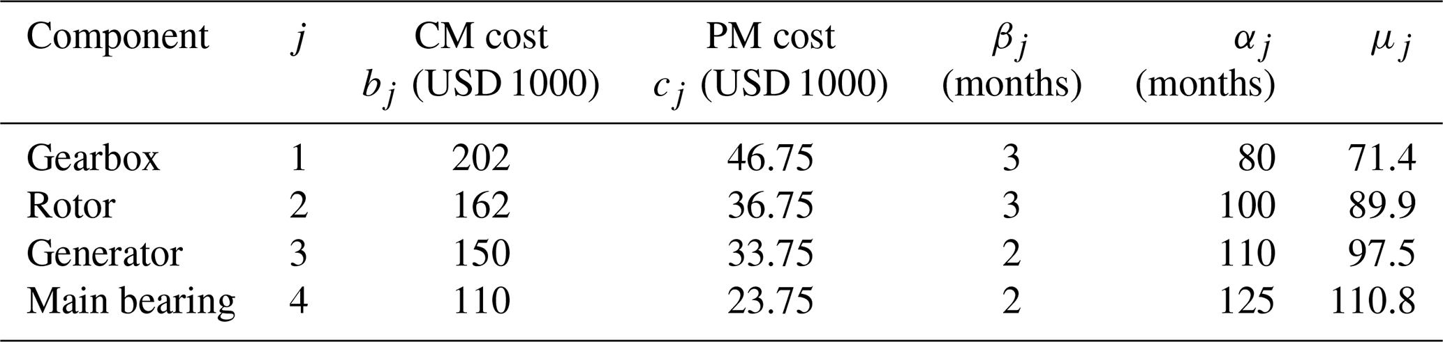
The three case studies analyzed in this section treat a wind turbine as a system represented by four components. They are all based on the parameter values taken from the paper Tian et al. (2011) (see Table 1), where the cost unit is USD 1000 and the time unit is 1 month. The lifetime of the wind turbine is assumed to be 30 years. This implies the parameter value T=360 months. As to other model parameters, it is assumed that

s=0, which implies that all four components initially are as good as new;

r=60 months – see Sect. 4.1 for motivation; and

λ=3, based on Gustavsson et al. (2014).

Comparing the characteristics of four wind turbine components shown in Table 1, it is important to observe a strict ordering from the perspective of the associated PM costs. For example, consider components 1 and 2. The rightmost column says that the expected life length of the gearbox is smaller by 18.5 months, which on its own suggests a higher rate of replacements for the component 1. But even the other two parameters, CM cost and PM cost, are ordered in a way b₁>b₂, c₁>c₂, which is favorable for more frequent replacements of component 1 compared to component 2.

Table 1 Key parameters for a four-component system.

All computational tests are performed on an Intel 2.40 GHz dual-core Windows PC with 16 GB RAM. The mathematical optimization models are implemented in AMPL IDE (version 3.5); the model components (Eqs. 10 and 7) are calculated by MATLAB (version R2015b), and then the optimization problems are solved using CPLEX (version 12.8).

4.1 Study 1: focusing on a single component at a time

If n=1, d_t≡d, and s=0, the objective function (Eq. 5) takes the form

$$\begin{array}{}\text{(22)}& f\left(\mathit{x}\right)=\sum _{t=\mathrm{1}}^{r+\mathrm{1}}{a}_t{x}_t,a_t={\displaystyle \frac{d+c_t}{t}},\end{array}$$

where given a sequence of independent random variables $L_i\stackrel{d}{=}L$ with L having a Weibull (α, β) distribution,

$$\begin{array}{}\text{(23)}& c_t=c+E\left(\sum _{i=\mathrm{1}}^{\mathrm{\infty }}{\mathrm{1}}_{\left\{L_{\mathrm{1}}+\mathrm{\dots }+L_i\le t\right\}}\left[b+d-{\left({\displaystyle \frac{L_i}{t}}\right)}^{\mathit{\lambda }}(c+d)\right]\right).\end{array}$$

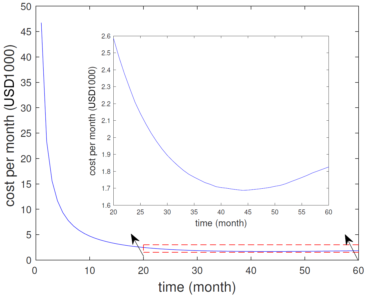
In the single component setting, coefficient a_t in Eq. (22) describes the monthly maintenance cost if the next PM is planned at time t (assuming that at time 0 the component was as good as new). In this section, we analyze the behavior of the function a_t under some realistic model parameters. It turns out, in the current setting, that minimizing the objective function (Eq. 5) is equivalent to minimizing a_t over t=1, …, r+1, and, moreover, the constraint (Eq. 7) can effectively be disregarded. As a result of this analysis, we propose r=60 months as a practical length of the planning period for our algorithm.

Figure 4 presents a typical profile for the monthly maintenance cost a_t as a function of the time t of the next PM planned activity. The inset of Fig. 4 clearly shows that the best time for next PM is at τ=43 given the mobilization cost of d=USD 5000. The maintenance cost in this case is a₄₃=USD 1700 per month.

Figure 4 Monthly maintenance cost for the gearbox with the mobilization cost d=5000.

The same value τ=43 can be also seen on the lowest among four lines depicted on Fig. 5 if parameter d, shown on the horizontal axis, takes a value of 5. The gearbox line on Fig. 5 displays larger values of τ for higher mobilization costs d. The same pattern is seen for the other three components taken one at a time.

Now we are ready to explain how the results of our analysis justify the proposed value r=60 months for the length of the next PM planning period. The ideal choice of r must satisfy two contradicting requirements. On the one hand, r should not be very small to avoid too many NextPM steps in Algorithm 1 advising for no PM activities during the next planning period. On the other hand, a smaller value of the parameter r would significantly reduce the computational time of the NextPM model. As a compromise solution, we choose r in such way that at least one PM activity is expected to be scheduled during the planning horizon. Since gearbox is expected to be replaced most often, referring to Figs. 4 and 5, we take the value of r=60 months for our case studies.

Figure 5 The optimal next PM time τ as a function of the mobilization cost d for different single-component systems.

4.2 Study 2: seasonal effects

In this section, we study how different mobilization costs d_t result in different optimal PM schedules. Part A presents a baseline study of a pure CM strategy with no PM activities. Part B deals with seasonally changing d_t around the average value $\stackrel{\mathrm{‾}}{d}=\mathrm{USD}\mathrm{10}\mathrm{000}$. Part C takes up a similar case with a lower average mobilization cost $\stackrel{\mathrm{‾}}{d}=\mathrm{USD}\mathrm{5000}$.

4.2.1 Part A

Consider the simplest wind turbine maintenance strategy when the PM option is ignored and a CM activity is performed whenever a turbine component breaks down. This baseline case study will help us to evaluate how much can be saved by introducing PM planning.

Table 2 Summary of the NextPM results for $\stackrel{\mathrm{‾}}{d}=\mathrm{USS}\mathrm{10}\mathrm{000}$.

The total cost associated with the pure CM strategy is estimated based on the random number of failures over the time interval [0, T] for all n components

$$\begin{array}{}\text{(24)}& \begin{array}{rl}F\left(T\right)& =\sum _{j=\mathrm{1}}^{n}E\left(\sum _{i=\mathrm{1}}^{\mathrm{\infty }}{\mathrm{1}}_{\left\{V_i^j\le T\right\}}\left(d_{V_i^j}+b_j\right)\right)\\ & =\sum _{j=\mathrm{1}}^n\underset{\mathrm{0}}{\overset{T}{\int }}\left(d_u+b_j\right)d{H}_j\left(u\right),\end{array}\end{array}$$

where H_j are the corresponding renewal functions

$$\begin{array}{}\text{(25)}& H_j\left(t\right)=E\left(\sum _{i=\mathrm{1}}^{\mathrm{\infty }}{\mathrm{1}}_{\left\{V_i^j\le t\right\}}\right),t>\mathrm{0},j=\mathrm{1},\mathrm{\dots },n.\end{array}$$

According to the standard renewal theory (see for example Grimmett and Stirzaker, 2020), for large values of T,

$$\begin{array}{}\text{(26)}& {\displaystyle \frac{F\left(T\right)}{T}}\approx \sum _{j=\mathrm{1}}^n{\displaystyle \frac{\mathrm{1}}{T{\mathit{\mu }}_j}}\underset{\mathrm{0}}{\overset{T}{\int }}\left(d_u+b_j\right)du=\sum _{j=\mathrm{1}}^n{\displaystyle \frac{\stackrel{\mathrm{‾}}{d}+b_j}{{\mathit{\mu }}_j}},\end{array}$$

where

$$\stackrel{\mathrm{‾}}{d}={\displaystyle \frac{d_{\mathrm{1}}+\mathrm{\dots }+d_T}{T}}.$$

Applying this approximation to the four-component model of the wind turbine, the monthly maintenance costs for the pure CM strategy are computed to be USD 7396 for $\stackrel{\mathrm{‾}}{d}=\mathrm{USD}\mathrm{5000}$ and USD 7618 for $\stackrel{\mathrm{‾}}{d}=\mathrm{USD}\mathrm{10}\mathrm{000}$.

4.2.2 Part B

To address the seasonal effects of the mobilization costs d_t, the following mobilization costs (in thousands of USD) for different months in a year are used.

Jan	Feb	Mar	Apr	May	Jun	Jul	Aug	Sep	Oct	Nov	Dec
15	13	11	9	7	5	5	7	9	11	13	15

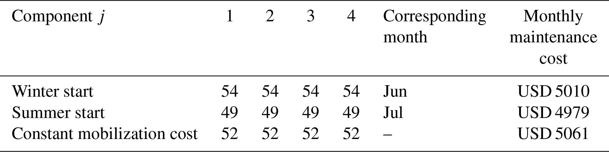
It is assumed that the mobilization costs for different months are different, but for the same month in different years they are the same. In this case, the average mobilization cost is $\stackrel{\mathrm{‾}}{d}=\mathrm{USD}\mathrm{10}\mathrm{000}$. The given monthly costs are based on a discussion with the experts affiliated with the Swedish Wind Power Technology Centre (SWPTC). Table 2 summarizes the results produced by the NextPM algorithm applied to the following three settings:

Winter start scenario.

If the wind turbine starts functioning in January, then the mobilization costs d_t (in thousands of USD) follow the following periodical dynamics over time t=1, 2, …:

$$d_{\mathrm{1}}=\mathrm{15},d_{\mathrm{2}}=\mathrm{13},\mathrm{\dots },d_{\mathrm{12}}=\mathrm{15},d_{\mathrm{13}}=\mathrm{15},d_{\mathrm{14}}=\mathrm{13},\mathrm{\dots }$$

Summer start scenario.

If the wind turbine starts functioning in July, then the mobilization costs d_t are taking the values (in thousands of USD):

$$d_{\mathrm{1}}=\mathrm{5},d_{\mathrm{2}}=\mathrm{7},\mathrm{\dots },d_{\mathrm{12}}=\mathrm{5},d_{\mathrm{13}}=\mathrm{5},d_{\mathrm{14}}=\mathrm{7},\mathrm{\dots }$$

Constant mobilization cost scenario.

This scenario has no seasonal effect in that for each month t, the mobilization cost d_t is the same: d₁=10, d₂=10, d₃=10, … (in thousands of USD).

Our results suggest (as a consequence of high mobilization costs) performing PM to all four components at a certain time, irrespective of the scenario. With the summer start setting, the average monthly maintenance cost is somewhat lower. Notice that in all of the seasonal settings, the proposed PM activities are scheduled for summer months (having lower mobilization costs). Observe that all three monthly averages (USD 5010, 4979, 5061) are much lower than the baseline value USD 7618 obtained in Part A.

4.2.3 Part C

In this section, the mobilization costs are halved to contrast the results of Part B, so that $\stackrel{\mathrm{‾}}{d}=\mathrm{USD}\mathrm{5000}$ and d_t take the following values (in thousands of USD) depending on which month of the year lies behind the time parameter t.

Jan	Feb	Mar	Apr	May	Jun	Jul	Aug	Sep	Oct	Nov	Dec
7.5	6.5	5.5	4.5	3.5	2.5	2.5	3.5	4.5	5.5	6.5	7.5

The new results presented in Table 3 are drastically different from the results of Part B.

Table 3 Summary of the NextPM results for $\stackrel{\mathrm{‾}}{d}=\mathrm{USD}\mathrm{5000}$.

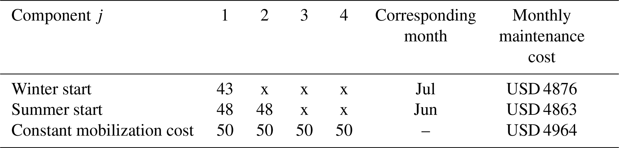
According to Table 3, in the winter start setting, the optimal next PM plan suggests a PM activity on month 43 only for component 1, the gearbox. With the seasonal mobilization cost, the next PM is always planned during the summer since the mobilization cost is low then. Again, the most economic among the three scenarios is to start in the summertime, with the optimal plan being to perform the next PM activity on month 48 by replacing the components 1 and 2.

Table 4 Outputs of the NextPM and PMSPIC models for d=USD 1000.

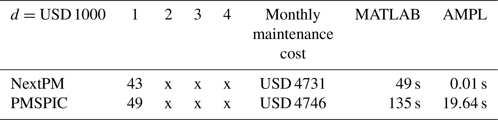
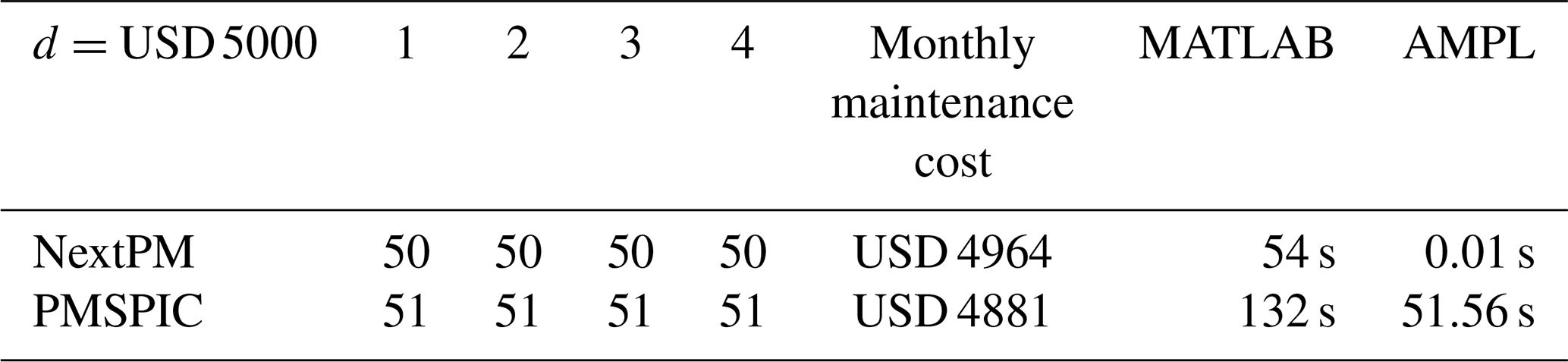
Table 5 Outputs of the NextPM and PMSPIC models for d=USD 5000.

Table 6 Outputs of the NextPM and PMSPIC models for d=$10000.

The optimal times for the next PM activity have landed in the range between 43 and 50 months and seem to be quite short. This is explained by the particular choice of the model parameters presented in Table 1: under the assumption of independence between the lives of the four components, the average time until the first failure is slightly below 50 months. (Notice that in this case study, the estimated parameters for the components' life lengths are based on the data collected for wind turbines from year 1994 to 2004. For the modern wind turbines, the mean survival times will be longer.) Another important contributing factor is the assumption of low PM costs, with higher PM costs the optimal next PM activity would be scheduled at a later time. In the special case with equal PM and CM costs, the optimal solution is to forget about PM planning and fully rely the pure CM strategy.

Comparison of the results of Part B and Part C with those of Part A shows that implementation of the PM planning reduces maintenance costs by 35 %.

4.3 A performance comparison with PMSPIC

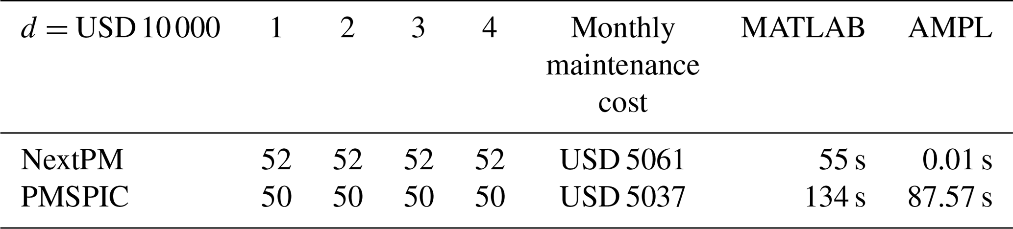
In this case study, we compare the outputs of the NextPM model and the optimization model PMSPIC. A comparison of the NextPM model with the PMSPIC model is not a straightforward exercise, since the latter produces a maintenance plan for the whole lifespan [0, T] of the multi-component system in question. To make a fair comparison, we characterize both approaches in terms of the time average maintenance costs. The following three tables summarize the results for three values of the constant mobilization cost d:

Tables 4–6 reveal that the next PM schedules produced by NextPM and PMSPIC are quite similar. The observed small differences in the maintenance costs do not imply that PMSPIC gives better solutions, since NextPM calculates the maintenance costs within a different modeling framework. The main advantage of NextPM compared to PMSPIC is in the computational speed. The effectiveness of the algorithms is reported in the two rightmost columns. The “MATLAB” column gives the time it takes to generate the main parameters of the model. For the NextPM the number of parameters is much smaller, and they are $c_{s,t}^j$, $D_{s,t}^j$. The “AMPL” column gives the time it takes to solve the optimization model. For example, if d=USD 10 000, the NextPM optimization runs 10 000 times faster than the PMSPIC optimization.

For d=USD 5000, the NextPM calculations are performed with the time unit being 3 d. The results are rather similar to those obtained for the time unit 1 month. Solving this problem with AMPL has required a time increase from 0.01 to 0.08 s caused by a 10-fold increase of the number of the time steps. The corresponding increase in the AMPL time for the PMSPIC model was much more dramatic: it takes more than 11 h to solve the full optimization problem.

5 Conclusions

This article introduces a new NextPM optimization model aiming at PM scheduling for a wind turbine viewed as a multi-component system. Which of the components should undergo PM replacements first is decided based on the information on the component ages. Compared to the PMSPIC model from Gustavsson et al. (2014) that generates a maintenance plan for the whole lifetime of the wind turbine, the NextPM model produces an optimal schedule only for the next PM activity. By focusing on a shorter planning horizon and implementing a different model structure, we succeeded in substantially reducing the computational time.

NextPM is tested with three case studies based on the data for four components of the wind turbine taken from Tian et al. (2011). Under the seasonal variation, our results show that PM activities should be always scheduled in the summertime. This is due to the lower mobilization costs during the summer months. When the NextPM model is compared to the pure CM strategy, it is found that around 35 % of the maintenance costs can be saved by applying the NextPM model. The third case study compares the performances of NextPM and PMSPIC algorithms, demonstrating the accuracy of the NextPM model despite being much less complex than PMSPIC.

In this paper our NextPM model is applied to a system of four components belonging to a single wind turbine. However, we claim that our approach can handle the case of, say, 10 turbines with 80 components in total (the computational time required by our algorithm grows linearly with the increased number of components, while PMSPIC's computational time grows exponentially fast).

The notable limitation of our setting is that it neglects such important maintenance activities as inspections and minor and major repairs. By considering full replacements as the only kind of CM and PM activities allowed in the model, we were able to tame the mathematical challenge of the problem in hand. Still, even within this simplified model framework, our computational analysis may bring useful insights of more efficient PM planning, depending on a few key parameters of a concrete wind farm. Our results should be viewed as a first promising step towards a much more sophisticated mathematical optimization model that would take into account available condition monitoring data and even recognize the difference in the failure rates for minor repairs, major repairs, and component replacements.