the Creative Commons Attribution 4.0 License.
the Creative Commons Attribution 4.0 License.
 | 24 Oct 2022
Observer-based power forecast of individual and aggregated offshore wind turbines
Frauke Theuer
Andreas Rott
Jörge Schneemann
Lueder von Bremen
Martin Kühn
Due to the increasing share of wind energy in the power system, minute-scale wind power forecasts have gained importance. Remote-sensing-based approaches have proven to be a promising alternative to statistical methods and thus need to be further developed towards an operational use, aiming to increase their forecast availability and skill. Therefore, the contribution of this paper is to extend lidar-based forecasts to a methodology for observer-based probabilistic power forecasts of individual wind turbines and aggregated wind farm power. To do so, lidar-based forecasts are combined with supervisory control and data acquisition (SCADA)-based forecasts that advect wind vectors derived from wind turbine operational data. After a calibration, forecasts of individual turbines are aggregated to a probabilistic power forecast of turbine subsets by means of a copula approach. We found that combining the lidar- and SCADA-based forecasts significantly improved both forecast skill and forecast availability of a 5 min ahead probabilistic power forecast at an offshore wind farm. Calibration further increased the forecast skill. Calibrated observer-based forecasts outperformed the benchmark persistence for unstable atmospheric conditions. The aggregation of probabilistic forecasts of turbine subsets revealed the potential of the copula approach. We discuss the skill, robustness and dependency on atmospheric conditions of the individual forecasts, the value of the observer-based forecast, its calibration and aggregation, and more generally the value of minute-scale power forecasts of offshore wind. In conclusion, combining different data sources to an observer-based forecast is beneficial in all regarded cases. For an operational use one should distinguish between and adapt to atmospheric stability.
- Article
(4641 KB) - Full-text XML
- BibTeX
- EndNote


With the increasing share of wind and solar power in our energy system, the need for accurate minute-scale power forecasts to support grid stability and electricity trading arises (Dowell and Pinson, 2016; Sweeney et al., 2020; Würth et al., 2019). The low geographical dispersion of installed offshore wind capacity and its consequently high volatility (Malvaldi et al., 2017) call for skilful forecasts of, in particular, offshore wind power. Commonly, statistical methods, such as the benchmark persistence or AR(I)MA (auto-regressive (integrated) moving average) methods, are applied on those timescales (Würth et al., 2019). While those methods are reliable in many situations, they underperform, for instance, during ramp events, i.e. sudden and strong changes in wind speed or direction. Therefore, recently remote-sensing-based wind speed and power forecasts have been researched as a physical-based alternative (Würth et al., 2018; Valldecabres et al., 2018b, a, 2020; Theuer et al., 2020b, 2021; Pichault et al., 2021).
Several studies have shown the potential of lidar-based wind speed and power forecasts to outperform the benchmark persistence under specific atmospheric conditions (Valldecabres et al., 2018b; Theuer et al., 2021; Pichault et al., 2021). Theuer et al. (2020b) and Valldecabres et al. (2018b) found that atmospheric stability can influence forecast accuracy in particular with respect to the wind speed height extrapolation. Theuer et al. (2021) showed that overall lidar-based forecasts are more accurate during stable conditions; however, they can only outperform persistence during unstable stratification because persistence is also more skilful during stable situations. Valldecabres et al. (2020) introduced a dual-Doppler radar-based forecast that was able to outperform persistence in terms of probabilistic scores during ramp events and for free-stream turbines. Two lidar-based methods, one based on a neural network and one on a smart persistence approach, introduced by Pichault et al. (2021) were able to exceed persistence, as well as an ARIMA method during ramp events and non-ramp situations, for different wind directions and atmospheric conditions onshore. In their work the authors focus on deterministic forecasts and wind farm power forecasts that do not distinguish forecasts at turbine level.
Driven by these promising results, the methods' development now needs to be directed towards an operational use. Besides the fact that there are many situations during which persistence outperforms the lidar-based forecast, low forecast availability is a main issue with the technology and concepts available so far. Hence, depending on the wind farm layout, scanning trajectories, lidar availability and wind conditions, no or only low-quality forecasts can be generated (Theuer et al., 2020b). This problem can be reduced by optimizing scanning trajectories, increasing the lidar's measurement range and possibly commissioning additional devices. However, during situations with reduced lidar sight due to, for example, fog or rain or when devices fail, one would need to fall back to an alternative data source. For that purpose, hybrid methods are worth being considered. In the context of lidar-based methods, Theuer et al. (2021), for instance, showed that the additional use of wind turbine operational data can contribute to the forecast accuracy. Also Pichault et al. (2021) included wind farm operational data in the form of a smart persistence approach in their forecast and achieved promising results.
Currently, lidar-based methods have been evaluated with regard to their probabilistic characteristics in a few cases only (Theuer et al., 2020b) but mainly with respect to their deterministic characteristics and for individual wind turbines (Würth et al., 2018; Valldecabres et al., 2018b; Theuer et al., 2021). However, for end-users in power trading and system operation, uncertainty information is of high value as it aids decision-making processes (Dowell and Pinson, 2016; Sweeney et al., 2020). One way to increase the reliability and sharpness of probabilistic forecasts is statistical post-processing, i.e. forecast calibration (Thorarinsdottir and Gneiting, 2010). Commonly, ensemble model output statistics (EMOS) is used. EMOS was first developed for temperature and pressure forecasts (Gneiting et al., 2005) but has successfully been applied to the prediction of precipitation (Scheuerer, 2014), wind speed (Thorarinsdottir and Gneiting, 2010), wind vectors (Schuhen et al., 2012) and power (Späth et al., 2015).
Considering the different areas of application of minute-scale forecasts, both individual turbines' power output and aggregated wind farm power or power at the grid connection point, i.e. aggregated power of a subset of individual wind turbines, are important. While the former are mainly required for wind turbine control (Würth et al., 2019), the latter are of interest for trading and system operation purposes. So far, lidar-based forecasts of individual wind turbines focused on free-stream situations. In a next step, these methodologies need to be extended to wake-influenced turbines. A main challenge is hereby the propagation technique, which assumes constant wind vector trajectories and is therefore unable to account for wakes. Valldecabres et al. (2020) circumvent this by applying a directional turbine efficiency that significantly improved the skill of their radar-based forecast.
Individual turbines' power forecasts can also be helpful when determining wind farm power. In this context, recently hierarchical forecasting on both temporal and spatial levels has gained attention, aiming to achieve coherency between different levels of the hierarchy and thereby improving forecast performance at each level (Bessa, 2016; Gilbert et al., 2020). A common method in the context of coherent probabilistic forecasts is copula approaches. Gilbert et al. (2020) successfully implemented and tested a variety of copulas to aggregate the probabilistic power forecasts of individual wind turbines to the probabilistic forecast of wind farm power.
Our objective in this paper is to develop a probabilistic observer-based forecast of aggregated wind farm power. To do so, we first introduce an observer-based power forecast of individual wind turbines that combines lidar and turbine operational data. This method accounts for variable wake conditions and increases forecast availability and skill. Additional calibration further improves the forecast's probabilistic characteristics. In the second step, we aggregate individual probabilistic wind turbine power forecasts to probabilistic wind farm power forecasts by applying a copula approach.
The basis of this work is the lidar-based forecasting approach introduced and analysed in more detail in Theuer et al. (2020a, b, 2021). The method is briefly described in Sect. 2.1. In this work this approach is significantly extended further as described in the following. Using SCADA (supervisory control and data acquisition) data, it is first extended to an observer-based forecast (OF) to increase forecast availability and skill (see Sect. 2.2). In a next step, observer-based forecasts are calibrated by means of ensemble model output statistics (EMOS) (see Sect. 2.3). Finally, probabilistic power forecasts of individual wind turbines are aggregated using different copula approaches (see Sect. 2.4).
2.1 Reference method lidar-based forecast (LF)
The reference method probabilistic lidar-based power forecast (LF) using single lidar measurements was developed by Theuer et al. (2020b) and is based on the work of Valldecabres et al. (2018a) who applied dual-Doppler radar. Lidar-based power forecasts utilize horizontal or slightly elevated plan position indicator (PPI) lidar scans measuring the inflow of an offshore wind farm. Typically, lidar devices are positioned on the transition piece (TP) of a wind turbine or alternatively a nearby platform and record line-of-sight (LOS) wind speed measurements and the carrier-to-noise ratio (CNR) at each scanned azimuth angle and range gate along with a time stamp. Using that information, lidar scans are filtered applying a data density approach on normalized CNR values and LOS wind speed measurements similar to Beck and Kühn (2017). By means of a velocity azimuth display (VAD)-like fit, the wind direction χ is then determined dependent on range gate r (Werner, 2005) and used to reconstruct a wind field with the horizontal wind speed uh from the line-of-sight wind speed measurements uLOS and the lidar's azimuth angle ϑ:
After wind field reconstruction, the individual lidar scans are interpolated to a Cartesian grid and synchronized in time (Beck and Kühn, 2019). Time synchronization refers to the propagation of individual parts of the lidar scans measured at different times to the same time step using semi-Lagrangian advection. It aims at accounting for the large time shift within each scan. A Lagrangian advection technique is then applied to propagate wind vectors, i.e. horizontal wind speed and wind direction information at each grid point. Hereby, it is assumed that vectors travel with their local wind speed and wind direction and do not change their trajectory while travelling. Wind vectors reaching the area of influence around the target turbine within a time interval of k±30 s with lead time k are selected to contribute to the target turbine's probabilistic forecast. For each forecasted time step, wind data recorded during a time interval previous to forecast initialization are taken into account. That means that for each forecast several time-synchronized scans are considered, and the travelling time of wind vectors can therefore exceed the lead time. Considering also previous scans is important to be able to forecast turbines positioned further away from the lidar-scanned area. Wind speed forecasts at measurement height um are transformed to hub height assuming a logarithmic stability-corrected wind speed profile (Emeis, 2018). Here, we apply a methodology introduced as tendency-based forecast in previous work (Theuer et al., 2021). It determines the wind speed tendency at measuring height and applies it to wind speed at hub height uhh after performing a correction of measuring height zm and atmospheric conditions defined by the Obukhov length L and the roughness length z0 between time steps ti and ti−1 (see Eq. 2). Ψ(z,L) describes the stability correction term (Emeis, 2018). Measuring heights vary along the range gate due to the curvature of the Earth and dynamically due to a thrust-dependent tilt of the lidar device (Rott et al., 2022). The hub height wind speed at the future time step ti is then defined as
In a final step, the wind speed forecast is transformed to a power forecast using power curves extracted individually for each wind turbine from 1 min mean SCADA wind speed and power data. In this case, the wind speed values are not measured but estimated from power, pitch angle and the SCADA system's turbine power curve.
Details on this forecasting methodology can be found in Theuer et al. (2020b, 2021).
2.2 Extension to an observer-based forecast (OF) by integrating a SCADA-based forecast (SF)
If the LF is invalid due to missing data, the prevailing wind conditions, the lidar trajectory or wind farm layout, one needs to fall back to an alternative forecasting approach. For that purpose we introduce the observer-based forecast, which combines the LF and a SCADA-based forecasting approach.
The SCADA-based power forecast (SF) modifies the methodology introduced in Rott et al. (2020), adapting its wind vector weighting approach and timescales to match the LF. The 1 Hz wind speed and wind direction data of all wind turbines of the wind farm are propagated using Lagrangian advection. In accordance with the LF, only wind vectors v arriving within a certain area of influence around our target turbine j are selected. The selected vectors originating at time tv,j are then weighted according to their age using an inverse temporal distance weighting to determine the weighting factor :
with
and the tuning parameter p∈ℕ that determines the strength of the weighting factor's decrease with increasing temporal distance (Rott et al., 2020). The selected wind vectors are resampled to a predefined number of wind vectors with their individual contribution given by the weighting factor. As suggested by Rott et al. (2020) a bias correction with the observed wind speed uobs,j and the ensemble average of the forecast at turbine j, i.e. , is applied to all members v of the forecast at this turbine to account for possible systematic errors and wake effects. The bias-corrected wind speed vectors then yield
with Nt the number of time steps with length Δτ prior to forecast initialization t−k, with lead time k, considered to determine the bias. Wind speed forecasts are transformed to power forecasts as described for the LF (Sect. 2.1).
In this work we extend the LF to an observer-based power forecast (OF) by integrating the SF. If both LF and SF are valid, they are weighted equally in the OF; otherwise only the valid forecast is considered. To be considered valid we require a minimum number of wind vectors to reach the target turbine for both methods. In that way, we avoid individual wind vector outliers being given too much weight. To account for the varying number of wind vectors contributing as a consequence of different temporal and spatial resolutions of the lidar and SCADA data, we resample each forecast to contain the same predefined number of members.
2.3 Calibration of the observer-based forecast
In a next step, the OF is calibrated using ensemble model output statistics (EMOS). EMOS is commonly used to calibrate ensemble forecasts; in our work it is applied to minute-scale remote-sensing-based power forecasts for the first time. Hereby, a truncated Gaussian distribution,
for and and with rated power Pr is used to model the wind speed distribution (Thorarinsdottir and Gneiting, 2010). The probability density function of the standard normal distribution is defined by ϕ and its cumulative distribution function (cdf) by Φ. The mean μi,j,
and the variance of the distribution,
are modelled as a linear function of the ensemble mean and variance , respectively, with time index i and turbine index j as suggested by Thorarinsdottir and Gneiting (2010). The cdf of the ensemble members at time i and for turbine j is defined as and referred to as Fi,j in the following. The parameters a, b, c and d are optimized to minimize the cost function,
based on the continuous ranked probability score (crps) of the forecast,
with the observation xi,j, the number of time steps considered Nc and the Heaviside step function H (Gneiting et al., 2007). A sliding window approach is applied; thus a training interval with optimized length before forecast initialization is used to calibrate the forecast.
2.4 Aggregated wind turbine power forecast using a copula approach
The observer-based forecast provides probabilistic power forecasts of individual wind turbines, i.e. one cdf Fi,j for each time index i and individual wind turbine j. Here, we aim to derive a joint predictive distribution of wind power production from a subset of wind turbines in a wind farm using a copula approach following the work of Gilbert et al. (2020) and Bessa (2016). In our work we apply the method to a data set with higher temporal resolution and shorter forecast horizon. This approach is based on Sklar's theorem, which states that a m-dimensional cumulative distribution F, with the number of turbines m and the length of the training data set tn, can be expressed using a copula function C of the individual marginal distributions Fi,j as
conditional on well-calibrated forecasts with uniformly distributed marginals uj=Fj(xj) (Gilbert et al., 2020). In this work, we apply a Gaussian copula,
with the m-dimensional normal distribution ΦΣ with covariance matrix Σ and a mean of . To determine the joint predictive distribution of the individual turbines and finally the probabilistic aggregated power, we proceed as follows. First, marginal distributions of all wind turbines to be considered for the aggregation are determined from the cdfs and observations as , and their uniformity is verified (Pinson et al., 2009). Marginals are then transformed into the Gaussian domain described by . Based on these transformed and normally distributed marginals, the covariance matrix Σ of the training data set can be determined. This multivariate distribution can be used to generate M random samples, which are then transformed back to the uniform domain. Finally, for each turbine j and time step within the test data set i, the samples are transformed into the power domain using its cdf Fi,j and summed over all turbines to yield a set of aggregated power samples. Based on these M aggregated power samples, a power distribution, i.e. a probabilistic forecast, can be derived.
To enlarge the test data set, we estimate covariance matrices using a sliding window approach. This also allows us to determine a joint predictive distribution that flexibly adapts to changing atmospheric conditions. A change in wind direction, for example, will affect the wake situation of the turbines and is consequently expected to have an impact on the turbine subset's joint distribution too.
In addition to the empirical covariance determined as described above, we define and test parametric covariance matrices based on an exponential relation,
with the covariance between two turbines Σj,h and the spatial distance Δr between the position of turbines j and h (Gilbert et al., 2020). The parameter ν is fitted using a least-squares regression and the empirically determined covariance matrix. The advantage of parametric copulas is their lower sensitivity to reduced data availability, avoiding noisy covariances and overfitting (Gilbert et al., 2020).
We further evaluate vine copulas as a more flexible option compared to Gaussian copulas. Vine copulas describe a set of bivariate copulas with variable distribution families for each (turbine) pair (Bessa, 2016). Here, we determined vine copulas using the MATLAB framework developed by Coblenz (2021). Distribution families are chosen using the Akaike information criteria (AIC) (Aas et al., 2009).
After the general description of the methodological steps in the previous section, we introduce the case study analysed in this work and its case-specific parameters in Sect. 3.1. In Sect. 3.2 the results of the LF and SF for individual wind turbines are presented. Further, we assess the value of the OF compared to the LF, SF and persistence (Sect. 3.3) and evaluate the calibrated OF compared to the raw, i.e. the uncalibrated, one (Sect. 3.4). Finally, we determine the forecast skill of the aggregated probabilistic power of several wind turbines and compare it against a probabilistic version of persistence (Sect. 3.5).
3.1 Case study at the offshore wind farm Global Tech I (GT I)
The methodology described in the previous sections is applied to and evaluated at the offshore wind farm Global Tech I (GT I) in the German North Sea. The wind farm consists of 80 turbines of type Adwen AD 5-116, with a hub height of zhh=92 m, a rotor diameter of D=116 m and a rated power of Pr=5 MW. The lidar was placed on the transition piece of turbine GT58 at a height of zTP=24.6 m. Horizontal plan position indicator (PPI) lidar scans were performed with a WindCube 200S (serial no. WLS200S-024) and with an elevation of 0∘, an azimuth angle spanning 150∘, an azimuthal resolution of 2∘, range gates from 500 to 7950 m in 35 m intervals and an accumulation time of 2 s. Including the measurement reset time, the scanning duration was 156 s. The scanning trajectories, which were adjusted manually according to four wind direction sectors, and the wind farm layout are depicted in Fig. 1. Figure 1a additionally depicts the layout of the wind farms Albatros and Hohe See, which were under construction but not yet operational during the time of the analysis. Those turbines did not cause any wakes but were visible as hard targets in the lidar scans occasionally, which were omitted during data filtering and thus did not impact the forecast. More details on the measurement campaign are available in Schneemann et al. (2020) and Theuer et al. (2020b, 2021).

Figure 1Layout of the wind farm Global Tech I with turbine positions visualized as black dots. Further, the neighbouring wind farms Albatros (+) and Hohe See (×) are shown. The lidar location is depicted as a red diamond and lidar trajectories as coloured dashed lines. The Cartesian grid is centred around the lidar's position. Grey horizontal lines mark turbine rows referred to in this work. The blue rectangle indicates the zoomed-in region shown on the right. It displays turbine numbers of the wind farm's centre region.
Each forecasted time step of the LF considered the six most recent scans and thus can contain wind data measured during the last 15 min. This ensures that also turbines positioned far away from the lidar scans can be reached by low wind speeds, and their forecasts will not be biased. Wind vectors contributing to the SF were weighted using a tuning parameter of p=4. The choice of this parameter is further discussed in Sect. 4.1. The SF's bias correction was performed considering a number of Nt=5 time steps prior to forecast initialization. This ensures that there is enough data for bias estimation while keeping the correlation high. The step length was chosen as Δτ=156 s in accordance with that of the lidar scans. LF and SF were generated with an area of influence of 2 D and a minimum of 20 required wind vectors (Theuer et al., 2021) and were resampled to contain 500 members. Forecast calibration was performed with a 5 h training interval before forecast initialization. The time window was optimized in a sensitivity analysis. A calibration was only performed for situations with at least 60 % valid data within that training period.
To construct a joint predictive distribution of all turbines of GT I a sufficiently large training data set with simultaneously available forecasts of all turbines is required. As a consequence of the limited forecast availability, we therefore only considered subsets of turbines to generate and evaluate aggregated power forecasts in this work. Turbine subsets were selected based on the availability of simultaneously available forecasts and their proximity to each other (see Fig. 1b). Here, a 6 h training window was used, again determined using a sensitivity analysis.
For forecast calibration, training of the copula and forecast evaluation, 1 Hz SCADA power data, averaged to 1 min intervals, were used.
3.2 Evaluation of lidar-based and SCADA-based power forecasts for individual wind turbines
We evaluate 5 min ahead power forecasts generated within the period 8 March to 21 June 2019 against 1 min mean SCADA data. In total, 9438 valid forecasts were generated, and 6753 were successfully calibrated. Hereby, we considered only situations during which both lidar and SCADA data were available for forecast generation and evaluation and persistence forecasts were available as a reference. The benchmark persistence assumes the future value equals the current observation. A probabilistic version of persistence was constructed by adding forecasting errors of the past 19 time steps to the current forecast as described by Gneiting et al. (2007). Further, forecasts of individual turbines not in normal operation mode were neglected. The wind conditions of the 9438 analysed time steps are summarized as a wind rose in Fig. 2. Wind speed and wind direction were extracted from the horizontal PPI lidar scans. The Obukhov length L reaches values as small as −27 m in unstable and 11 m in stable cases. Median values of L are −266 m for L<0 and 268 m for L>0. In the following analysis we will distinguish between stable (L>0) and unstable (L<0) atmospheric conditions in accordance with the definition of the stability-corrected logarithmic wind speed profile.
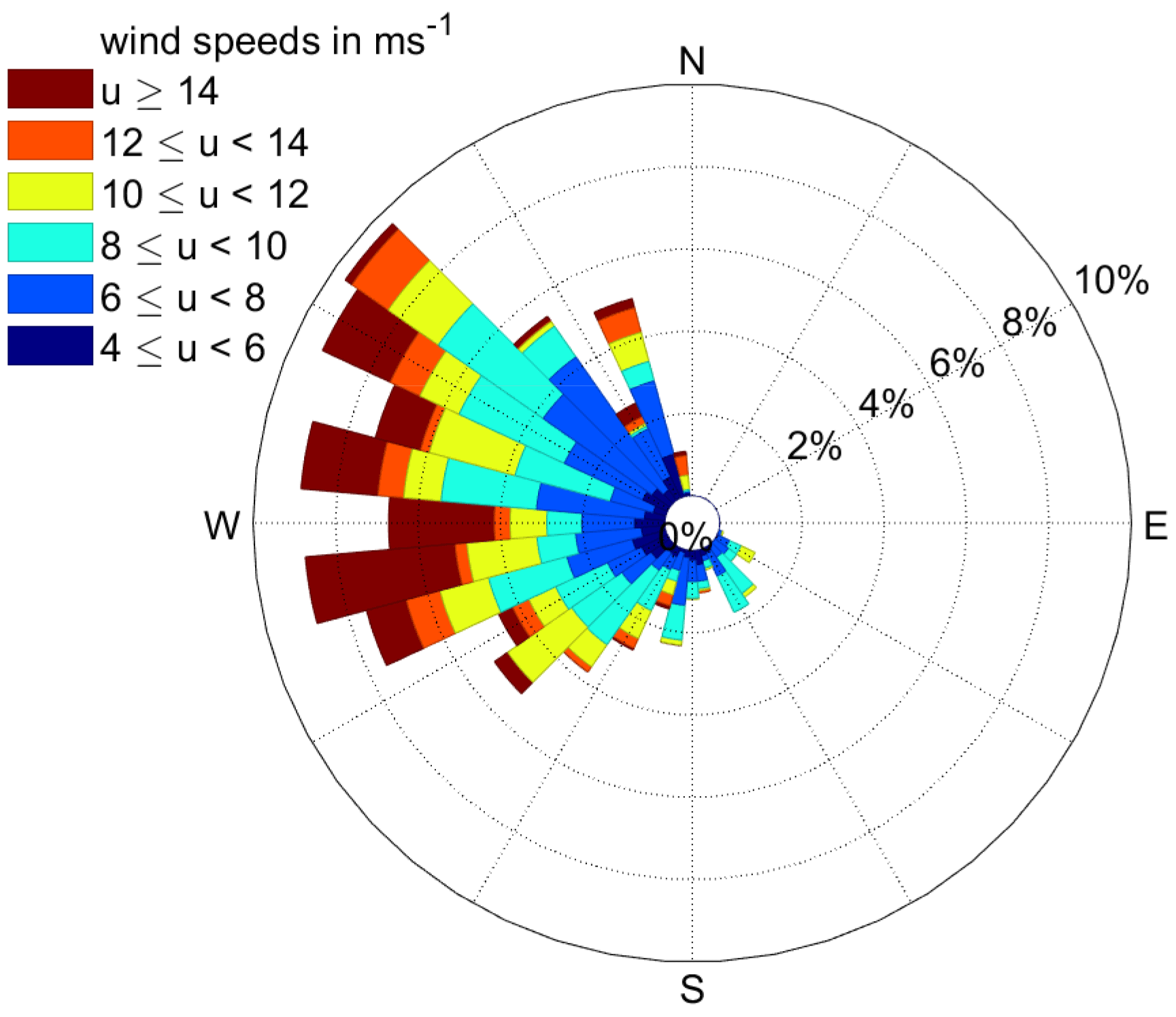
Figure 2Wind speed and wind direction distribution extracted from horizontal PPI lidar scans of the 9438 analysed time steps.
The forecast skill was determined by means of the average continuous ranked probability score:
To compare the skill of two forecasts the crps skill score (crps ss),
with the reference forecast is applied.
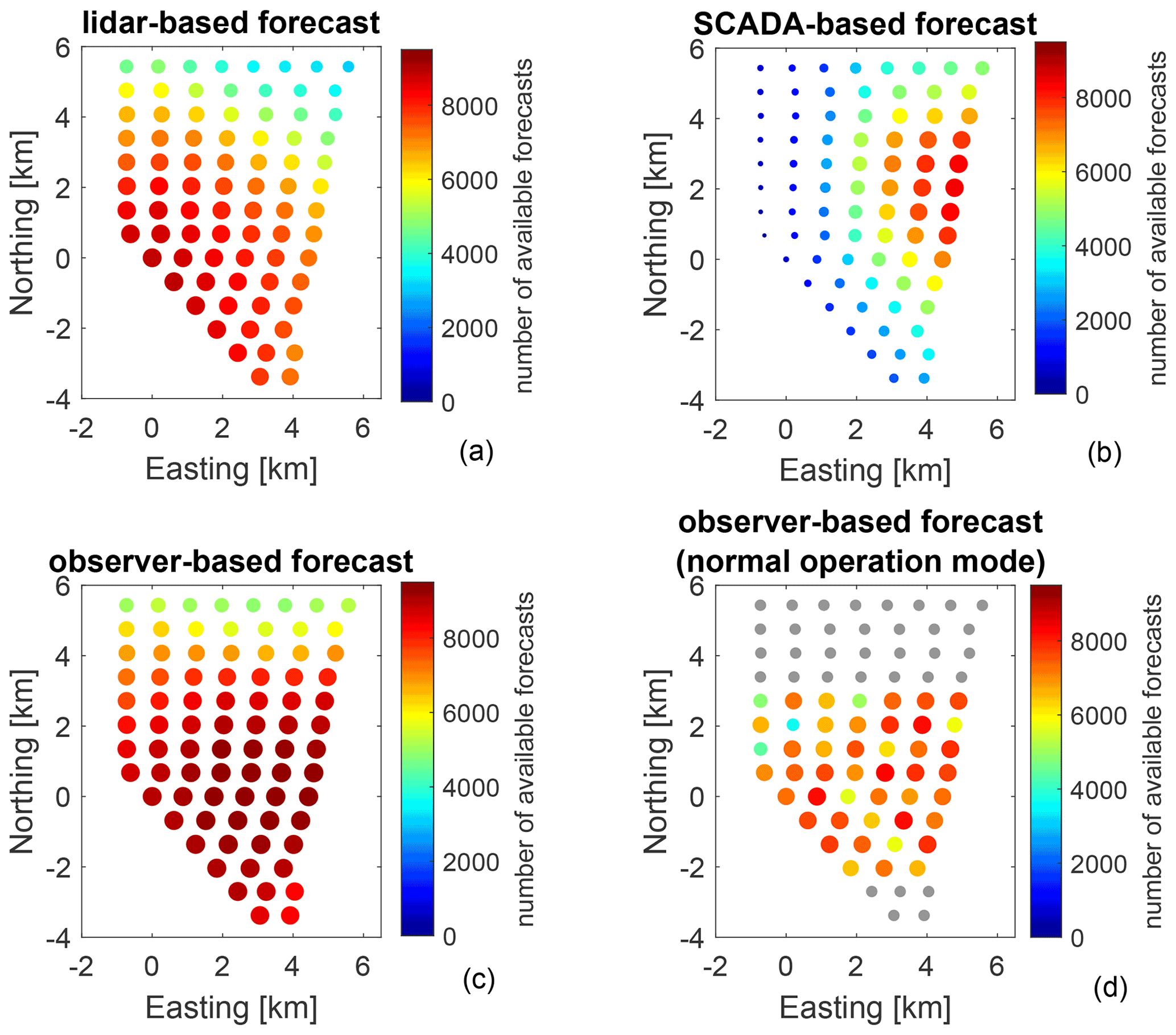
Figure 3Forecast availability for (a) the lidar-based forecast, (b) the SCADA-based forecast, (c) the observer-based forecast and (d) the observer-based forecast after filtering situations during non-normal operation. The subset of turbines shown in colours in (d) is analysed in more detail in this work, while turbines marked in grey are not considered for further analysis. The colour scale and magnitude of the dots visualize the number of valid forecasts.
To understand the impact of lidar coverage and turbine location on the forecast skill and forecast availability of LF and SF, we depict the number of available forecasts for each method in Fig. 3a and b. In Fig. 4 we further compare the crps ss of the LF and SF with persistence as reference for individual turbines of GT I and distinguish between unstable and stable atmospheric conditions. Based on the number of available forecasts the turbines GT30–GT75 (see Fig. 1) were selected for further analysis. Grey vertical lines mark horizontal wind turbine rows, with the turbine to the left of the line located on the easterly side of the wind farm.
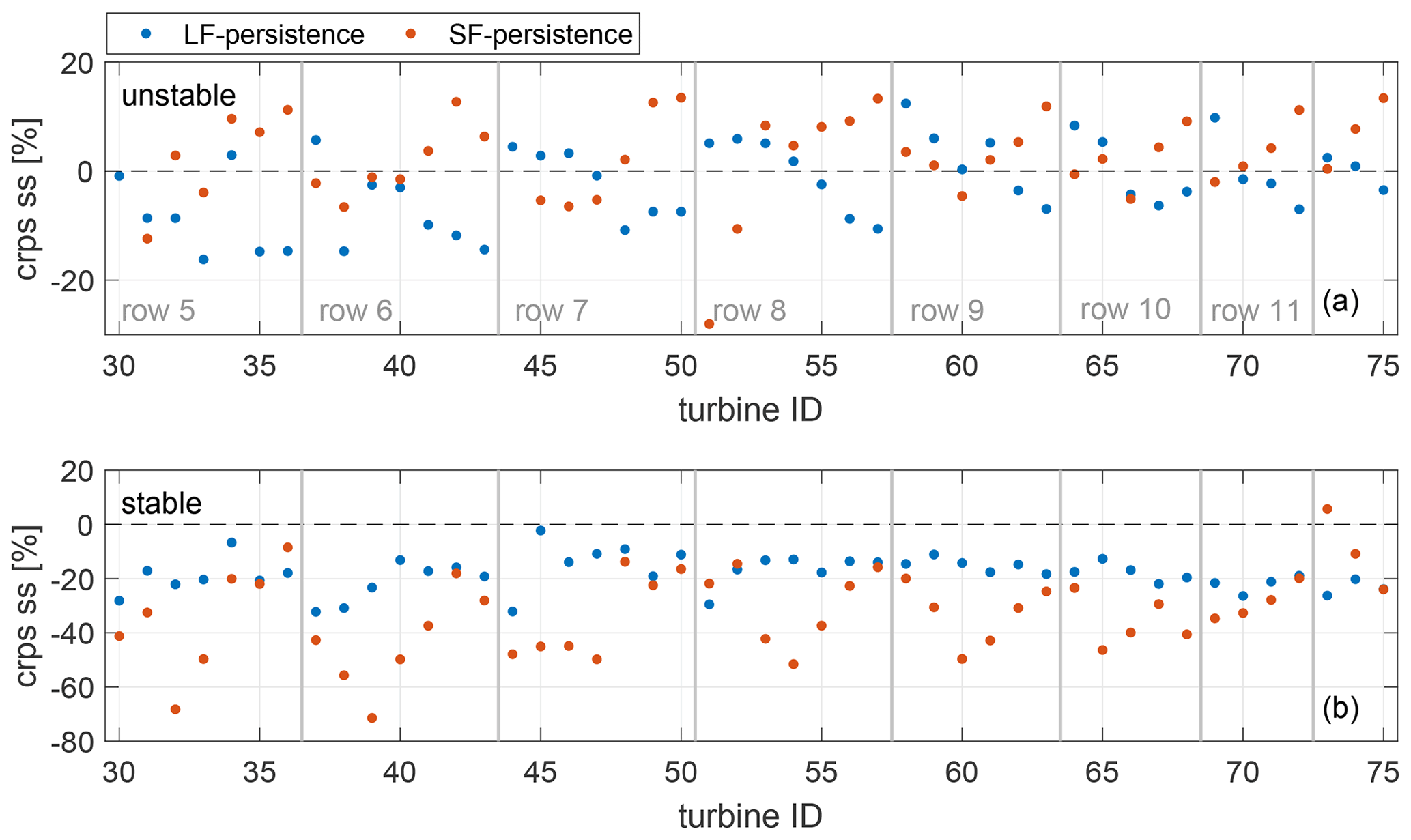
Figure 4The crps ss of LF and SF with persistence as reference for individual turbines of GT I and distinguishing between (a) unstable and (b) stable atmospheric conditions. Grey vertical lines mark horizontal wind turbine rows.
The westerly corner of the wind farm shows high LF availability (see Fig. 3a). In agreement with this, the LF was able to outperform persistence during unstable atmospheric conditions for those turbines covered well by the lidar scans (e.g. GT52, GT58, GT64). Its forecast availability is reduced for turbines located further away from the lidar. Here, also the forecast skill is low. This can be attributed to the longer time and distance wind vectors need to travel before reaching these turbines. Even though we consider in addition to the current lidar scan also previous ones, missing or low-quality scans increase the risk of wind vectors not reaching the turbines and negatively impact forecast skill. Moreover, high uncertainty might be related to wake effects. Wind turbines located in the northerly region of the wind farm show a low skill score due to insufficient lidar coverage. The SF mainly covers the easterly part of the wind farm and consequently performs well for easterly located turbines (e.g. GT50, GT57, GT63; see Fig. 4), also during unstable conditions. It cannot predict free-flow turbines, considering the main westerly wind direction, as no upstream turbines are available to propagate from. Hence, skill scores are lower for turbines positioned close to the first row. Overall, the results indicate that both methods are able to predict power of not only free-stream turbines but also wake-influenced turbines more accurately than persistence under unstable conditions. During stable stratification both methods fail, in particular the SF.
Other than the SF, the LF is not bias-corrected to account for systematic errors possibly related to wakes. We therefore consider it worthwhile to analyse the impact of wakes on the LF in more detail. To do so, the and the bias of GT30–GT75 are depicted in Fig. 5 for wind directions of 260–280∘ (Fig. 5a and b) and 170–190∘ (Fig. 5c and d). To capture in particular situations strongly impacted by wakes, we included only stable atmospheric conditions and situations operating below rated power (<0.9 Pr) in this analysis. The deteriorates, i.e. is growing, with increasing distance to the free-stream turbines. In accordance with the wind directions, forecasts are most accurate for westerly located turbines in Fig. 5a and for southerly located ones, with the exception of GT75, in Fig. 5c. The bias is not distinctly affected by the individual turbines' position in the wind farm and fluctuates closely around zero for westerly winds. For southerly winds, scores are generally slightly larger, and the bias of most turbines lies between 0.5 % and 1.5 %.
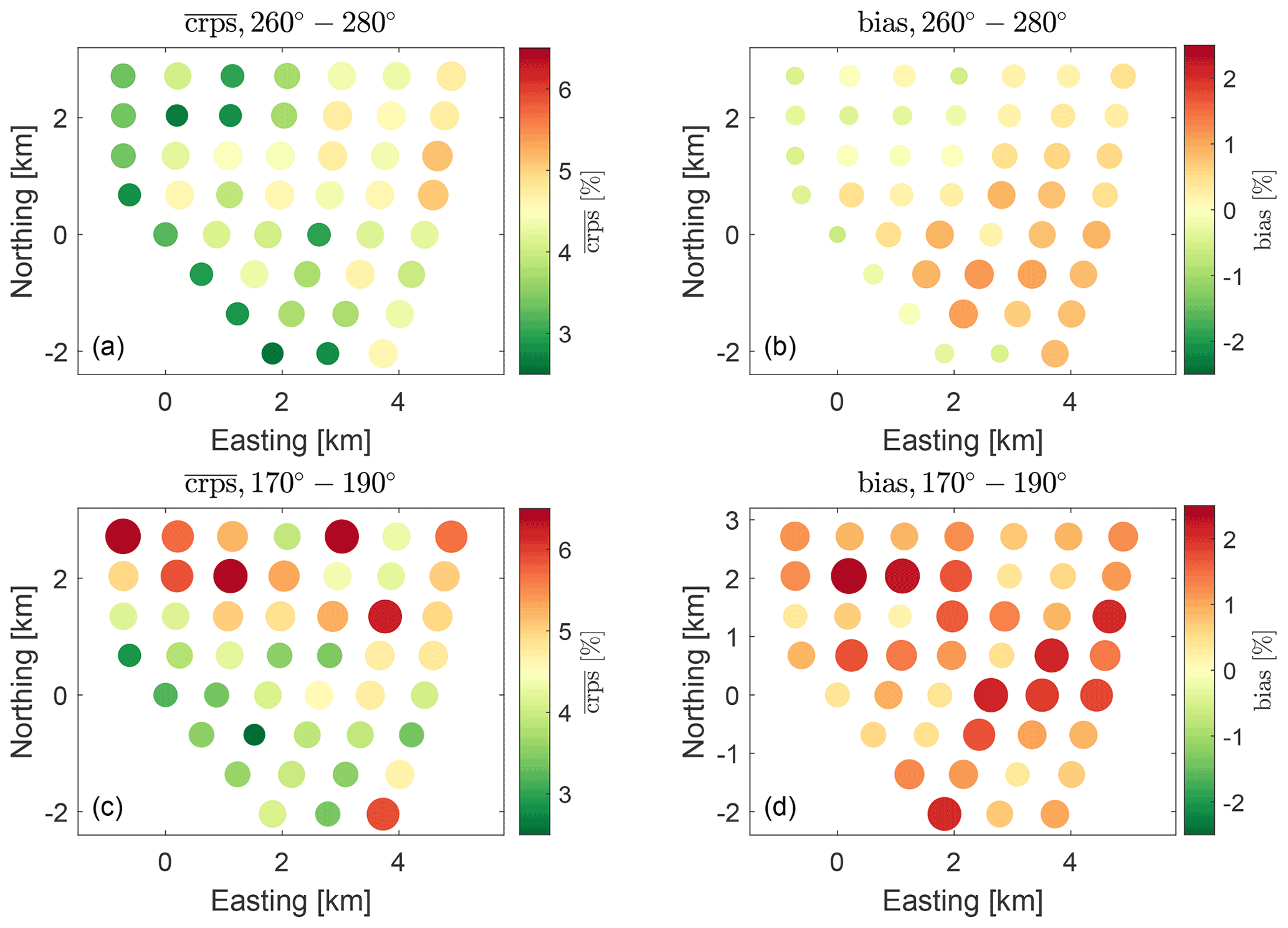
Figure 5The and bias of the LF for turbines GT30–GT75 in percent of rated power for stable atmospheric conditions, situations below rated power, and wind directions of (a, b) 260–280∘ and (c, d) 170–190∘. The colour scale and magnitude of the dots visualize the magnitude of the scores.
The LF's dependency on lidar coverage was already shown in previous work (Theuer et al., 2020b). Here, we focused on the SF's sensitivity to missing turbine data. In the case of failing measurement devices or maintenance operations, wind speed and wind direction information might be missing or inaccurate for some turbines during periods of time. Here, we analysed how the SF's forecast skill is affected by missing turbines. To do so, we randomly excluded an increasing amount of wind turbines as the origin of wind vector propagation for the whole analysed time period. We will refer to the number of turbines considered as turbine availability in the following. In Fig. 6 we compare the forecast availability and the normalized with respect to 100 % turbine availability for a number of exemplary turbines that have shown high forecast availability. The normalized in Fig. 6b only considers simultaneously available forecasts for all filter criteria. A reduction in turbine availability clearly causes a decrease in forecast availability and skill for all of the analysed turbines. The impact of missing turbines increases with lower turbine availability. For GT36, for instance, a reduction in turbine availability from 100 % to 50 % reduces the forecast availability to 97 % and increases the by 4.8 %. Further reducing turbine availability to only 25 % lowers the forecast availability by another 10.6 % and increases the by 11.5 %. A similar behaviour can be observed for turbines GT35 and GT42. Only for turbine GT56 do the forecast availability and change rather linearly.
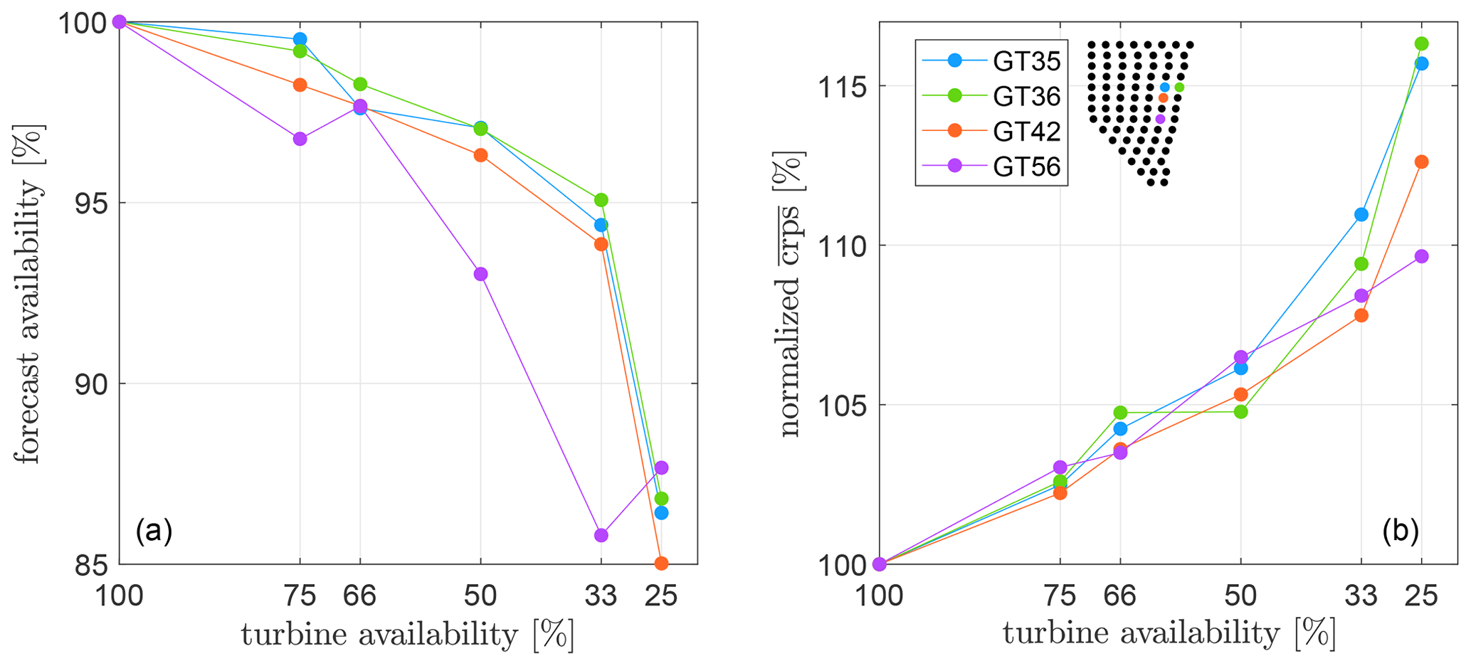
Figure 6(a) Forecast availability (in %) and (b) normalized with respect to 100 % turbine availability (in %) for reduced turbine availability and selected example turbines. The wind farm layout visualizes the turbines' positions.
3.3 Extension to an observer-based power forecast of individual wind turbines
A main advantage of the OF compared to the LF or SF is its increased forecast availability. This is visualized in Fig. 3, where the number of available forecasts for the 80 turbines of GT I for LF, SF and OF is shown. It becomes clear that the LF and SF complement each other well in terms of data availability (see Sect. 3.2) from which the OF can benefit. It shows high availability in the wind farm's centre, which decreases when approaching the north-westerly and south-easterly region of the wind farm. This is a consequence of lidar trajectories, wind farm layout and wind conditions at the site. The OF's availability for the selected turbines, GT30–GT75, after filtering turbines during non-normal operation (see Sect. 3.2) is depicted in Fig. 3d.
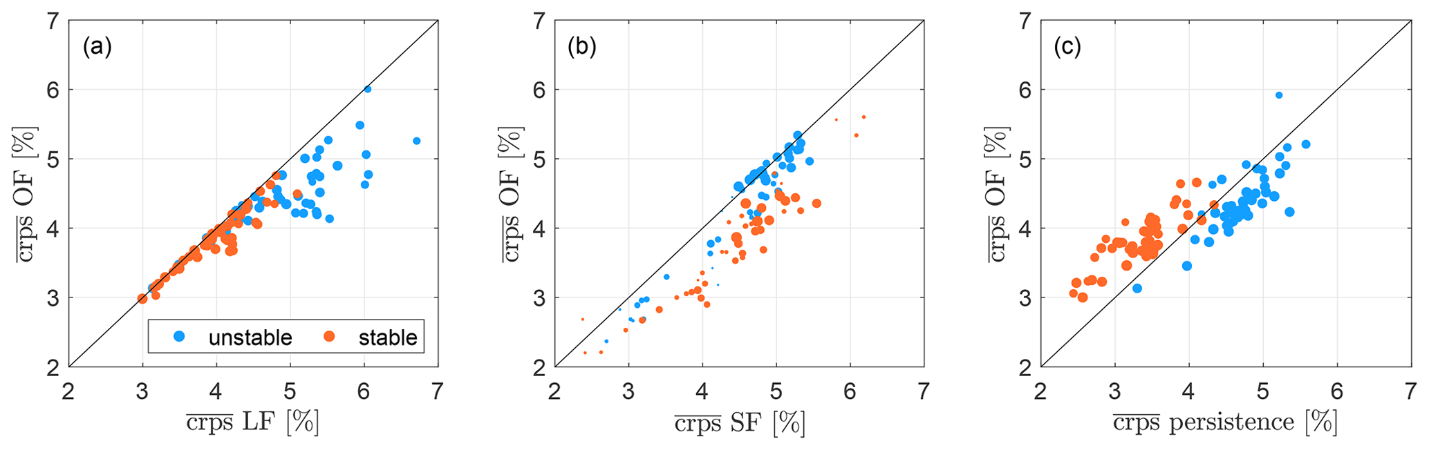
Figure 7Comparison of of the observer-based forecast to the (a) lidar-based forecast, (b) SCADA-based forecast and (c) persistence (% of the turbines' rated power). Each dot represents for one of GT I's wind turbines (GT30–GT75) both for stable and unstable atmospheric conditions. The dot size scales with the number of forecasts considered. Only situations with forecasts available for both methods are considered.
In addition to the forecast availability also the forecast skill can benefit from a combination of the two forecasting methodologies. Figure 7 depicts the for the OF compared to the LF, the SF and persistence for the 46 remaining turbines. To be able to compare OF and LF with SF we only consider situations for which both of the forecasts are available. That means that in Fig. 7a we only take those OFs into account that consist of either a combination of LF and SF or solely the LF. We distinguish between unstable atmospheric conditions (L<0) in blue and stable ones (L>0) in red. The dot size represents the number of available forecasts at the respective turbine and is scaled with the maximal value of available forecasts within each subplot. Data positioned below the diagonal black line indicates an improvement of the OF's forecast skill compared to the reference method.
In addition, in Fig. 8 we present the crps skill score for the individual wind turbines, distinguishing between atmospheric conditions for the same cases as visualized in Fig. 7. The OF shows higher forecast skill for all turbines in both stable and unstable situations compared to the LF. It benefits strongest from additional SFs for turbines located far away from the lidar scans, which are most affected by the LF's long wind vector travelling distances and times and possibly by wake effects. A number of turbines for which the effect almost disappears (e.g. GT44, GT51, GT58), indicated by dots positioned close to the diagonal line and a crps ss close to 0, are visible. Those correspond to free-stream turbines for which the amount of valid SFs is small and the OF consists mainly of LFs. Also compared to the SF, the OF's is improved for almost all analysed turbines. The effect is most distinct during stable atmospheric conditions and for turbines close to the free-stream region of the wind farm (e.g. GT39, GT54, GT60), thus with few upstream turbines for the SF available. Here, the SF can benefit strongly from additionally available lidar data. The OF is able to outperform persistence during unstable stratification for most turbines; however, it fails to do so during stable cases. Turbines for which the OF underperforms during unstable cases are positioned in the northerly region of the wind farm. Those located in the centre of the wind farm (e.g. GT50–GT58) can be forecasted best due to the beneficial data basis.
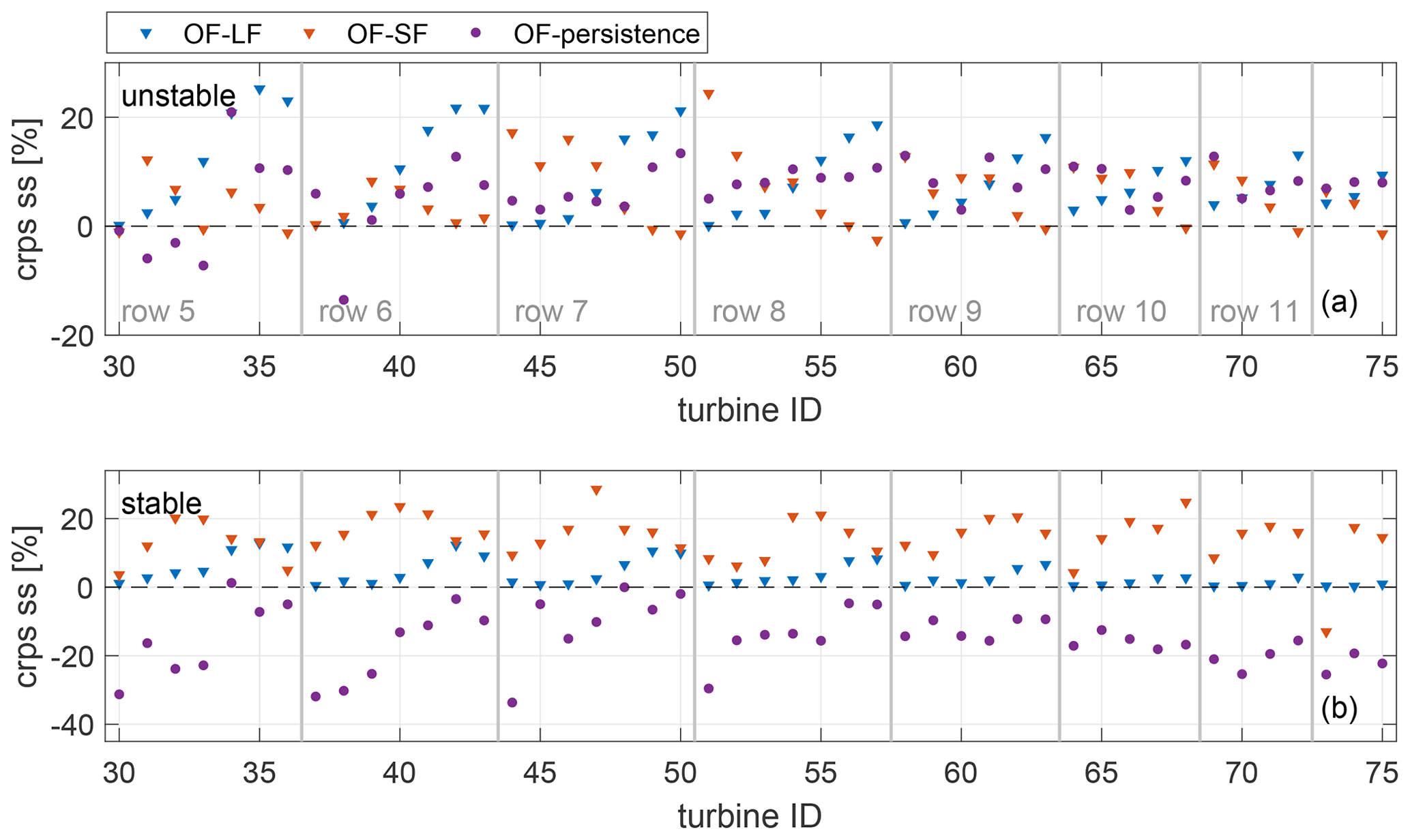
Figure 8The crps ss of the OF with LF, SF and persistence as reference for individual turbines of GT I and distinguishing between (a) unstable and (b) stable atmospheric conditions. Grey vertical lines mark horizontal wind turbine rows.
3.4 Calibration of observer-based power forecasts of individual wind turbines
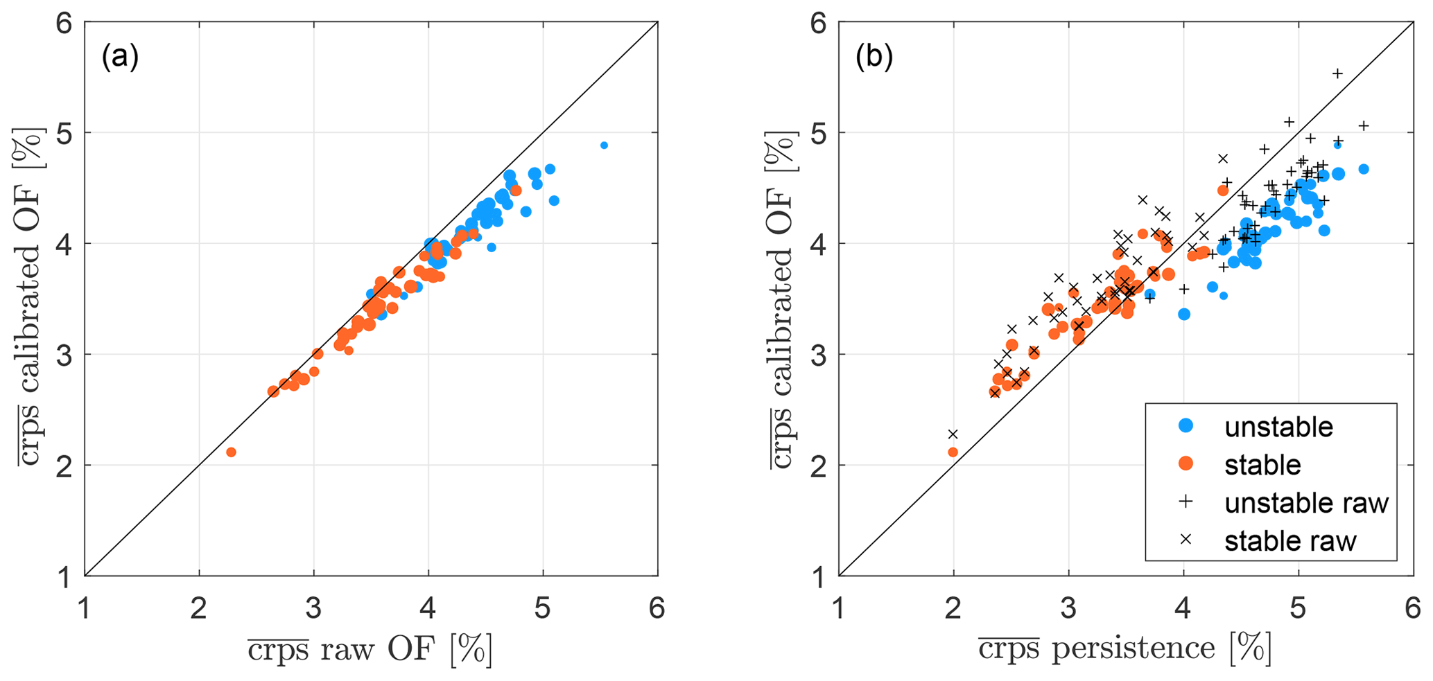
Forecast calibration aims to improve the probabilistic characteristics of forecasts. Moreover, well-calibrated forecasts are a prerequisite for the application of the copula approach (see Sect. 2.4). In Fig. 9a we therefore compare the of the raw and calibrated observer-based power forecast. As in Fig. 7, we distinguish between atmospheric conditions and scale the marker size according to data availability. For almost all of the analysed turbines the OF's skill was considerably improved by calibration. The effect seems most distinct for turbines with less accurate forecasts, which often coincide with lower data availability. A comparison of the OF and persistence in Fig. 9b reveals that persistence is outperformed only for few of the turbines during stable atmospheric conditions. However, the OF is now more skilful than persistence during unstable situations for all analysed turbines.
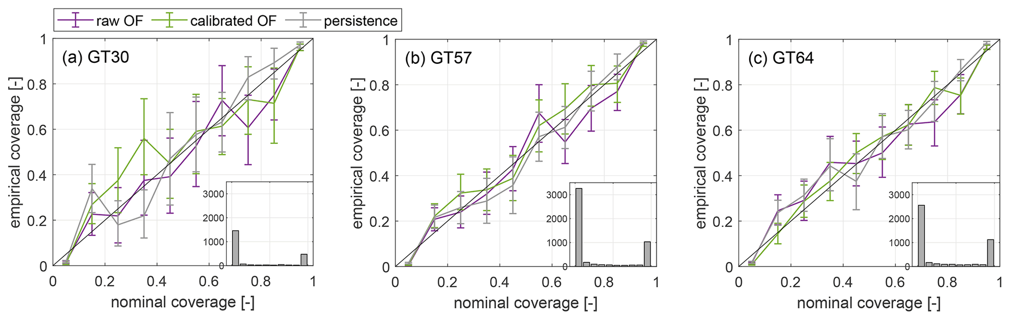
Figure 10Reliability diagrams of the raw observer-based forecast (purple), the calibrated observer-based forecast (green) and persistence (grey) for turbines GT30, GT57 and GT64. The 95 % confidence intervals are visualized as error bars. The diagonal black line indicates perfect reliability. Histograms show the number of valid forecasts per quantile step for the calibrated forecast.
In addition to we use reliability diagrams to evaluate the consistency between the statistics of the forecast and the observation. The reliability diagrams in Fig. 10 visualize the analysed quantile steps [0, 0.1, …, 1] on the x axis. For each time step the likelihood that a certain threshold is exceeded is determined from the forecast members and assigned to its specific quantile bin. The fraction of observations actually exceeding the threshold for those time steps is shown on the y axis. In this case, we define a threshold of 0.9 Pr. Accurate probabilistic forecasts of high-power regimes are particularly important for grid integration and trading. The 95 % confidence intervals of the reliability diagrams are determined by means of a bootstrapping approach and visualized as error bars. Due to the limited number of available forecasts, we did not distinguish between atmospheric stability when evaluating reliability diagrams.
To analyse differences in reliability dependent on turbine location we selected the exemplary turbines GT30, GT57 and GT64. The reliability diagram of GT30 fluctuates more strongly around the diagonal, and its confidence intervals are broad compared to GT57 and GT64. As visible in the histogram, this is related to a smaller number of valid forecasts, which in turn is a consequence of the turbine's location in the northerly region of the wind farm. In general, the data basis is too poor to draw any conclusions from comparing the different methods or turbine locations. Overall, the OF seems reasonably well calibrated.
3.5 Evaluation of aggregated wind turbine power forecasts
As explained in Sect. 3.1, the aggregation of individual turbines' power forecasts requires a large number of simultaneously available turbine forecasts. Furthermore, these individual forecasts need to be well-calibrated (Bessa, 2016). To have sufficiently large data sets that also allow for a distinction between atmospheric stability available we therefore limited our analysis to a maximum number of seven turbines per subset. Turbines within one subset were selected as those in close proximity to each other to increase the number of simultaneously available forecasts. To test the copula approach for a number of different circumstances, we selected subsets covering different parts of the wind farm, e.g. the westerly part in subset 1 and the easterly part in subset 3, and arranged in different shapes, e.g. an elongated turbine cluster stretching from the wind farm's south-westerly to north-easterly region in subset 2, a more dense cluster of turbines near the free-flow region in subset 4 or a horizontal wind turbine row in subset 5.
Table 1Turbine subsets, number of valid forecasts considered and (% of the subsets' rated power) for the vine, empirical and exponential copula approach and persistence for unstable and stable atmospheric conditions. The lowest scores are shown in bold.
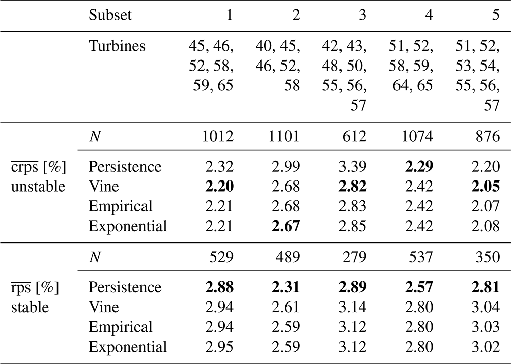
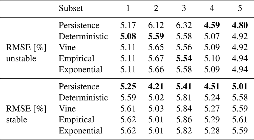
Table 2The RMSE (% of the subsets' rated power) for the vine, empirical and exponential copula approaches, the deterministic approach, and persistence for unstable and stable atmospheric conditions. The lowest scores are shown in bold.
In addition to probabilistic forecasts of aggregated wind turbine power, we also evaluated deterministic power forecasts using the root-mean-squared error (RMSE),
with forecasts fci and observations obsi with time index i and number of analysed forecasts N.
We generated deterministic forecasts of turbine subsets by aggregating deterministic forecasts of individual turbines and refer to this method as deterministic OF in the following. Deterministic forecasts of individual turbines were determined by averaging their ensemble members. Additionally, the ensemble members of the subsets' probabilistic power forecasts determined using the three different copula approaches, namely the empirical Gaussian copula, the parametric Gaussian copula and the vine copula (see Sect. 2.4), were averaged. The turbine subsets used, the number of valid forecasts considered within each subset, and the results for the different copula approaches and persistence are summarized in Tables 1 and 2 for unstable and stable atmospheric conditions. Further, reliability diagrams of all subsets and approaches are shown in Fig. 11. The average absolute difference between empirical and nominal coverage for quantile steps q and their number Nq is summarized as quantile mean absolute error (mae),
and is additionally shown in Fig. 11f.
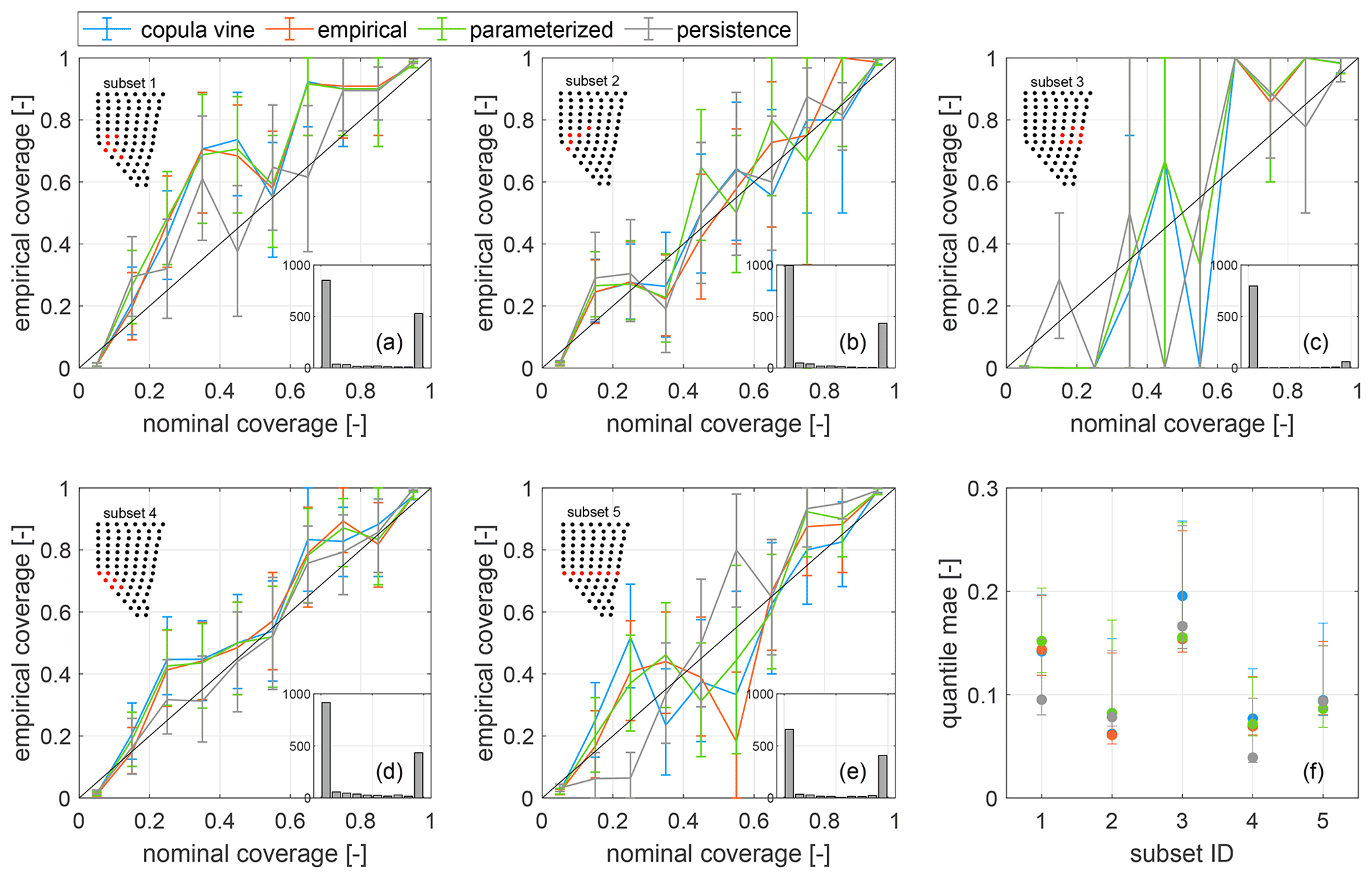
Figure 11(a–e) Reliability diagrams for the different turbine subsets (1–5) and copula approaches summarized in Table 1 and persistence. The turbine subsets are marked in red in the small wind farm layouts. Histograms show the number of valid forecasts per quantile step for the empirical copula approach. The diagonal black line indicates perfect reliability. In (f) the corresponding quantile maes are shown. For all subfigures 95 % confidence intervals are visualized as error bars.

Figure 12Average covariances of turbine subset 1 determined using the empirical (left: a, c, e, g, i, k) and exponential (right: b, d, f, h, j, l) copula approaches. Unstable (a, b) and stable (c, d) cases and situations with turbines operating below (<0.9 Pr) (e, f) and at rated power (≥0.9 Pr) (g, h) are compared. In (i)–(l) stable situations with turbines operating below rated power with wind directions ranging from 240–300∘ (i, j) and <240∘ (k, l) are depicted. The turbine subset 1 is marked in red in the small wind farm layout.
In terms of , four out of five subsets are able to outperform the benchmark persistence during unstable atmospheric conditions. For stable atmospheric conditions, persistence performs best. Generally, forecast skill is higher for the aggregated forecasts compared to those of individual turbines due to the smoothing of power fluctuation averaging. For three subsets unstable atmospheric conditions can be predicted more accurately than stable situations by all evaluated methods, contradicting previous results. A comparison of the different approaches and subsets with regard to their reliability and quantile mae is not conclusive, considering the overlap of the wide confidence intervals. This is a consequence of the small number of available forecasts. In terms of RMSE, the copula approaches are able to outperform persistence for three and the deterministic OF for only one of the evaluated subsets during unstable atmospheric conditions (see Table 2). During stable cases, persistence is most accurate for all five subsets. Overall, scores are very similar for the three tested approaches, and none of them can be identified as superior.
The analysis of the covariance matrices revealed their dynamic behaviour over time. The sliding-window approach allows the covariances to adapt to changing atmospheric conditions. In Fig. 12 we show average empirical and exponential covariance matrices of subset 1 for different conditions. We distinguish between atmospheric stability, average power production of free-flow wind turbines (GT30, GT37, GT44, GT51, GT58, GT64, GT69, GT73) and average wind direction of turbines GT30–GT75. We select covariances considering conditions during the 6 h time window used for copula training.
A comparison of empirical (left, Fig. 12a, c, e, g, i and k) and exponential covariance matrices (right, Fig. 12b, d, f, h, j and l) makes clear that covariances are smoothed by the parameterization. For exponential covariances, a distinct dependency on the turbines' spacing can be observed. Figure 12a–d show that, as expected, covariances are on average higher during stable atmospheric conditions than during unstable cases. In Fig. 12e–h we compare covariances of situations with turbines operating below rated power (<0.9 Pr) and those running at rated power (≥0.9 Pr). Slightly larger values can be observed below rated power. In Fig. 12i–l we analyse the covariances' dependency on wind direction. To exclude the impact of atmospheric stability and power production, we only consider cases with stable stratification and turbines operating below rated power here. To maximize the number of valid covariance matrices, relatively large wind direction intervals of 240–300 and <240∘ are chosen. Overall, covariances are higher for westerly winds as compared to south and south-westerly winds. We relate this mainly to changing wake situations. We exemplarily analyse the covariances' dependency on wind direction using turbine pairs GT45–GT46, GT45–GT52 and GT46–GT52. While for westerly winds the average covariance of GT45–GT52 is higher than that of GT45–GT46 and GT45–GT52, it is lower for south and south-westerly winds. This can be explained because for westerly winds, GT45 and GT52 experience similar wake conditions and are positioned approximately perpendicular to the incoming wind. In contrast, for south and south-westerly winds, their wake situation is different, with GT52 placed upstream of GT45. Here, GT45–GT46 and GT46–GT52 are subject to more similar wake effects and exhibit higher covariances. It should be noted that the number of covariance matrices considered for the different filter criteria varies considerably.
In the following, we review the lidar- and SCADA-based forecasting methodologies with regard to the impact of wakes and data availability. Further, the generation and calibration of the observer-based forecast, as well as the aggregation of individual power forecasts by means of a copula approach, are discussed. Finally, we assess the value of minute-scale power forecasts of offshore wind in a broader context.
4.1 Lidar- and SCADA-based power forecasts of individual wind turbines
In previous work (Theuer et al., 2020b, 2021) we have focused on the forecast of the first row of wind turbines, with respect to the main wind direction, only. Here, we extended the forecast to all wind turbines of the wind farm, also including waked wind turbines. Generally, the LF's skill is highest for free flow turbines and areas covered well by the lidar scans. As discussed in more detail in Theuer et al. (2020b), lidar range, scanning trajectory and wind farm layout do not only influence the forecast availability but can also impact forecast uncertainty and relate to, for example, a forecast bias. Our analysis has revealed that forecasting errors are larger for wind turbines and wind directions directly impacted by wakes, while a systematic over- or underestimation of wind speed was not observed. That means that the LF is generally able to capture the mean wake effect; however, it is not able to forecast small-scale fluctuations associated with it. The LF considers, just like persistence, past observations at the turbine of interest that are then multiplied with the wind speed tendency determined from lidar data (see Sect. 2.1). It is thus able to account for wakes to some extent. We assume that the higher errors observed are mainly related to turbulence in wake regions that cannot be represented well by Lagrangian advection. Furthermore, wind vectors reaching turbines positioned in the easterly and north-easterly region of the wind farm were typically propagated over a longer distance and time compared to turbines closer to the lidar scans. These vectors can be associated with higher uncertainty. For the SF, forecasts are most accurate in the region of the wind farm opposite to the prevailing wind direction, i.e. the north-easterly region. Here, the applied bias correction prevents systematic errors. Wind vector propagation of the SF is affected more strongly by wakes than the LF as it is performed at hub height. Also Valldecabres et al. (2020) accounted for wakes in their work by applying a directional turbine efficiency, which significantly improved their results. However, the forecast was only able to outperform persistence in terms of for wake-influenced turbines during ramp events.
The SCADA-based forecast introduced in this work is based on a high-frequency (0.2 Hz) flow reconstruction and prediction methodology developed by Rott et al. (2020). We extended this work to a probabilistic approach by resampling the selected wind vectors by also considering the weights assigned to them and included a power transformation. Rott et al. (2020) applied and validated their model to a high-frequency data set, aiming at applications in wind turbine control. In our work, we focus on 1 min mean forecasts with a temporal resolution of 2.5 min, in accordance with the lidar scans. Therefore, we adjusted the methodology to pre-select wind vectors following the lidar-based forecasting methodology, considering only those reaching an area of influence within a certain time window before applying the inverse temporal distance weighting. As opposed to Rott et al. (2020), we neglected the spatial distance weighting and relied solely on the temporal distance weighting, using a Shepard parameter of p=4. Rott et al. (2020) state that the usage of large Shepard parameters results in a more accurate representation of wind speed fluctuations, while lower parameters allow a robust forecast of average wind speeds. We chose a medium parameter as a good compromise between robustness and temporal resolution of wind speed fluctuations.
While the flow reconstruction method was applied only to forecasts with lead times up to 120 s, the results indicated that an application to forecasts with larger lead times might be valuable. Rott et al. (2020) showed that forecast accuracy decreases with lead time; however, its skill compared to persistence increases. Our results confirm the methodology's benefit compared to persistence for lead times of 5 min. Inaccurate wind direction data might impact the accuracy of SCADA-based forecasts. Wind direction was determined using the absolute yaw position and wind vane of each turbine, both of which are subject to uncertainties (Mittelmeier and Kühn, 2018; Simley et al., 2021). Rott et al. (2020) identified the model's approach to consider wakes and disturbances of the sonic anemometers and consequently wind direction measurements as additional sources of uncertainty.
The SF is able to account for missing data to some extent. It can thus be considered robust against the lack of data of individual wind turbines that might occur during daily operation of a wind farm due to maintenance or failing measurement devices. Only with more distinct reductions in turbine availability were forecast skill and forecast availability significantly reduced. In that case, gaps are too large, and important information is lost. How strongly missing turbine data impact forecast accuracy is also dependent on wind speed, wind direction and the target turbine's position. They could, just like insufficient lidar coverage, cause systematic forecasting errors.
4.2 Extension to an observer-based power forecast, forecast calibration and aggregation
The lidar- and SCADA-based forecasts complement each other well in terms of data availability. Further, the forecast skill of the observer-based forecast outperforms both individual methods. Our analysis clearly showed that both forecasting methods, LF and SF, profit from the additional data set considered in the OF. While we relate this mainly to an improved data basis for certain areas of the wind farm, a combination can also benefit from the individual forecasts' methodical differences. During unstable situations the SF was most significantly improved for turbines close to free-flow turbines due to significantly improved coverage. For stable stratification, the largest improvement shifts to turbines located further downstream. We relate this to more pronounced wake effects during stable stratification. As suggested previously, the LF is able to account for wakes more accurately than the SF (see Sects. 3.2 and 4.1), which means it can significantly increase the SF's value in such situations. For turbines located far away from the lidar, when propagated lidar wind vectors are associated with high uncertainty due to wakes and their increased propagation distance and time, the OF mainly benefits from more recent SCADA wind vectors.
It is common practice in (power) forecasting to combine different forecasting approaches to improve performance. Junk et al. (2015), for instance, combined different ensemble prediction systems to multi-model ensembles. They introduced different weighting approaches, namely implicit weighting, equal weighting and optimized weighting. The authors found that optimized weighting did not improve forecast calibration, while implicit weighting, which is based on the different number of ensemble members of the models, performed best. In our work, we were not able to apply implicit weighting as the number of wind vectors selected for the forecast strongly depends on the different spatial and temporal scales of the data sources. Future work should analyse how the different numbers of wind vectors reaching a certain turbine using the LF or SF can be considered in the weighting, thus moving from the equal weighting approach to a more implicit one.
Forecast calibration by means of ensemble model output statistics allows us to correct for systematic errors, as well as ensemble spread. By using a moving-time-window approach it is also possible to account for systematic errors varying with atmospheric conditions, for instance wind-direction-dependent wake losses. Varying atmospheric stability and turbulence intensity that might impact power fluctuations can be addressed by adapting the forecast spread.
As we were only able to aggregate a maximum of seven turbines, it is not yet possible to draw any conclusion regarding the copula approach's ability to predict the total wind farm power. Results indicate, however, that copulas can be a valuable tool to support the generation of probabilistic forecasts. Even though we generally expect persistence to have an advantage compared to observer-based methods for aggregated wind power forecasts as power fluctuations are averaged out, persistence underperformed for four out of five subsets in terms of during unstable conditions. The higher skill during unstable situations compared to stable ones for three of the analysed subsets contradicts previous results (Theuer et al., 2020b, 2021). It is likely related to a higher number of situations with turbines operating at rated power, which are associated with a higher forecast skill. Gilbert et al. (2020) applied a similar methodology to aggregate individual wind turbines' power forecasts and were also able to beat two benchmarks, namely a quantile regression model and an analogue ensemble method. However, their forecast's lead time was much larger, its temporal resolution was much lower, and a distinction between stability cases was not made, making a comparison difficult. The high temporal resolution of the OF might be one reason why covariances in our study are generally lower compared to the results of Gilbert et al. (2020). We found the magnitude of covariances to be dependent on atmospheric stability, turbine spacing, power production and wind direction. The small data set makes a more detailed distinction between different conditions difficult. Covariances are lower in situations with many power fluctuations, as expected during unstable atmospheric conditions and when turbines are subjected to wakes. Also for high-power regimes, when typically the ensemble spread is narrow, quantiles are less correlated, and thus the covariances are low. In cases where power forecasts and actual power production of neighbouring turbines can be expected to be rather similar, covariances are higher. This might happen due to more homogeneous wind fields upstream, typically during stable atmospheric conditions, and when the impact of wakes on the neighbouring turbines is similar.
An analysis of the RMSE revealed that for deterministic forecasts of turbine subsets it is more skilful to aggregate individual deterministic wind turbine forecasts. The comparison of different copula approaches suggests the use of an empirical or parametric copula instead of a vine copula. Vine copulas are more computationally expensive; however, they are able to achieve only marginally better results. Similar conclusions were drawn by Bessa (2016) and Gilbert et al. (2020). Results also varied for different turbine subsets. This is possibly related to different numbers of turbines considered, the different skill of the individual turbines' forecasts or varying distributions of atmospheric conditions within the data sets. For Sklar's theorem to hold, marginal distributions of forecasts need to be uniformly distributed. While our forecasts were reasonably well calibrated, further improvement would possibly also have benefits in the copula generation.
4.3 Future value of minute-scale offshore wind power forecasts
For future minute-scale forecasts of offshore wind power, considering, for example, the large number of wind farms in the North Sea and also their close proximity to each other, it might be beneficial to include operational data of several wind farms into the observer-based forecast. We expect that these additional data sources could further increase data availability, enhance forecast skill and in particular enlarge the forecast horizon. In such a case, however, one would need to carefully calibrate the forecast to include operational data from different wind farms. The availability of lidar-based forecasts could further be increased by deploying several lidar devices and by developing more powerful lidars, e.g. with considerably increased range or scanning speed. This might facilitate multi-elevation scans with a better resolution of the rotor swept area of future very large offshore turbines.
The forecast skill of lidar-based, SCADA-based and consequently observer-based forecasts is expected to decrease with increasing lead time as a consequence of assumptions made during Lagrangian advection as discussed in previous studies (Würth et al., 2018; Rott et al., 2020; Theuer et al., 2020b). An observer-based forecast covering large areas of, for example, the North Sea is therefore not expected to be able to forecast small-scale structures very accurately. However, it would likely be able to predict the occurrence of power ramps caused, for example, by passing fronts. It was shown in numerous studies and confirmed in this work that remote-sensing-based forecasts are able to outperform persistence in particular during unstable or turbulent situations and also during ramp events (Valldecabres et al., 2020; Theuer et al., 2021). We expect this to be true also for forecast horizons larger than 5 min, which we were restricted to in this work (Theuer et al., 2020b). The development of an early warning system of potentially grid-critical power ramps based on observer-based forecasts covering the North Sea is therefore considered a valuable extension to persistence. To this end, further analysis will investigate how the forecast skill for larger horizons compares to that of persistence during different conditions.
The overall value of observer-based forecasts compared to persistence for longer time periods will strongly depend on typical atmospheric conditions at the wind farm site. During stable atmospheric conditions forecasts are generally more accurate, but the OF is not able to outperform persistence (Theuer et al., 2021). In those cases, applying persistence should be considered instead or possibly a hybrid model that includes persistence (Theuer et al., 2022).
The aggregation of individual wind turbine power forecasts using a copula approach was strongly restricted by limited data availability in this work. As shown in other work (Valldecabres et al., 2018a; Theuer et al., 2020b) and previously discussed, the availability of forecasts is strongly dependent on lidar trajectories, wind farm layout and wind conditions. Excluding certain operating conditions of turbines further reduced the available data set. That means, in particular for a wind farm as large as Global Tech I, the generation of reliable simultaneously available forecasts for all turbines is difficult. Further analysis is required to evaluate how the proposed methods might benefit probabilistic power forecasts for wind farms of smaller size or with an overall higher forecast availability. Also trajectory optimization or the installation of multiple lidars instead of just one could improve the applicability of the copula approach. To evaluate the benefit of hierarchical forecasting these methods should also be compared to wind farm power forecasts that do not consider individual power forecasts on the turbine level (Pichault et al., 2021).
We developed an observer-based minute-scale offshore wind power forecast by combining a lidar-based and a SCADA-based approach. To improve probabilistic forecast skill we calibrated the observer-based approach. Further, a copula methodology was implemented to generate probabilistic power forecasts of aggregated turbine subsets.
Our results revealed the high potential of a complementary use of lidar-based and SCADA-based forecasts regarding both forecast availability and skill. We conclude that a combination of SCADA- and lidar-based forecasts is beneficial for all turbines in the wind farm and during both stable and unstable atmospheric conditions. Lidar-based forecasts were less skilful for wake-influenced turbines than for free-stream ones; however, they were able to predict the mean wake effect. SCADA-based forecasts were found to be very robust against reduced turbine availability. To guarantee high availability and skill of lidar-based forecasts a careful planning of lidar scanning trajectories is required, considering main wind direction, wind farm layout and lidar capabilities.
Forecast calibration was found to significantly reduce the forecasts' average crps; however, as a consequence of the small data set, no conclusions regarding the calibration's impact on reliability could be drawn. Even though forecast skill was significantly improved compared to the raw forecasts, calibrated observer-based forecasts were only able to outperform persistence during unstable rather than stable atmospheric conditions. Based on these results we conclude that for an operational use of the observer-based forecast a distinction between atmospheric conditions is useful. Given the current status of the methodology, during stable conditions it is recommended to rely on persistence. Also the use of a hybrid methodology might be beneficial and should be explored in the future. Applying the copula approach to generate aggregated probabilistic power forecasts for turbine subsets showed high potential. Empirical and parametric covariance matrices were found advantageous over vine copulas in particular considering their high computational cost. The copula approach was not able to add value to deterministic forecasts.
In future work the copula approach for probabilistic minute-scale power forecasting needs to be further analysed for wind farms with higher overall forecast availability.
Lidar and meteorological data are not published and can be made available on request. The OSTIA data set can be obtained from http://marine.copernicus.eu (Copernicus marine service, 2022). GT I SCADA data are confidential and therefore not available to the public.
FT conducted the main research and wrote the manuscript. JS conducted the measurement campaign, supported lidar data analysis, contributed to the scientific discussion and provided extensive feedback in the form of manuscript reviews. AR supported the development of the observer-based forecast, gave extensive feedback on copula and calibration methods and their mathematical formulation, and reviewed the manuscript. LvB and MK supervised the work, contributed to the scientific discussion and the structure of the paper, and thoroughly reviewed the manuscript.
The contact author has declared that none of the authors has any competing interests.
Publisher's note: Copernicus Publications remains neutral with regard to jurisdictional claims in published maps and institutional affiliations.
We acknowledge the wind farm operator Global Tech I Offshore Wind GmbH for providing SCADA data and thank them for supporting the measurement campaign in GT I and our work. We acknowledge the UK Met Office for making the OSTIA data set available. We thank Stephan Stone for conducting the measurement campaign and Marijn Floris van Dooren for numerous scientific discussions on the forecasting methodology.
This research has been supported by the Federal Ministry for Economic Affairs and Climate Action (OWP Control, grant no. 0324131A, WIMS-Cluster, grant no. 0324005, and WindRamp, grant no. 03EE3027A) and the Deutsche Bundesstiftung Umwelt (grant no. 20018/582).
This paper was edited by Sara C. Pryor and reviewed by two anonymous referees.
Aas, K., Czado, C., Frigessi, A., and Bakken, H.: Pair-Copula Constructions of Multiple Dependence, Insurance: Math. Econ., 44, 182–198, https://doi.org/10.1016/j.insmatheco.2007.02.001, 2009. a
Beck, H. and Kühn, M.: Dynamic Data Filtering of Long-Range Doppler LiDAR Wind Speed Measurements, Remote Sens., 9, 561, https://doi.org/10.3390/rs9060561, 2017. a
Beck, H. and Kühn, M.: Temporal Up-Sampling of Planar Long-Range Doppler LiDAR Wind Speed Measurements Using Space-Time Conversion, Remote Sens., 11, 867, https://doi.org/10.3390/rs11070867, 2019. a
Bessa, R. J.: On the quality of the Gaussian copula for multi-temporal decision-making problems, in: 2016 Power Systems Computation Conference (PSCC), 20–24 June 2016, Genoa, Italy, 1–7, https://doi.org/10.1109/PSCC.2016.7541001, 2016. a, b, c, d, e
Coblenz, M.: MATVines: A vine copula package for MATLAB, SoftwareX, 14, 100700, https://doi.org/10.1016/j.softx.2021.100700, 2021. a
Copernicus marine service: Copernicus Marine environment monitoring service, available at: http://marine.copernicus.eu/, last access: 19 April 2022. a
Dowell, J. and Pinson, P.: Very-Short-Term Probabilistic Wind Power Forecasts by Sparse Vector Autoregression, IEEE T. Smart Grid, 7, 763–770, https://doi.org/10.1109/TSG.2015.2424078, 2016. a, b
Emeis, S.: Wind Energy Meteorology, Springer, Cham, https://doi.org/10.1007/978-3-319-72859-9, 2018. a, b
Gilbert, C., Browell, J., and McMillan, D.: Leveraging Turbine-Level Data for Improved Probabilistic Wind Power Forecasting, IEEE T. Sustain. Energ., 11, 1152–1160, https://doi.org/10.1109/TSTE.2019.2920085, 2020. a, b, c, d, e, f, g, h, i
Gneiting, T., Raftery, A. E., Westveld, A. H., and Goldman, T.: Calibrated Probabilistic Forecasting Using Ensemble Model Output Statistics and Minimum CRPS Estimation, Mon. Weather Rev., 133, 1098–1118, https://doi.org/10.1175/MWR2904.1, 2005. a
Gneiting, T., Balabdaoui, F., and Raftery, A. E.: Probabilistic forecasts, calibration and sharpness, J. Roy. Stat. Soc., 69, 243–268, https://doi.org/10.1111/j.1467-9868.2007.00587.x, 2007. a, b
Junk, C., Delle Monache, L., Alessandrini, S., Cervone, G., and von Bremen, L.: Predictor-weighting strategies for probabilistic wind power forecasting with an analog ensemble, Meteorol. Z., 24, 361–379, https://doi.org/10.1127/metz/2015/0659, 2015. a
Malvaldi, A., Weiss, S., Infield, D., Browell, J., Leahy, P., and Foley, A. M.: A spatial and temporal correlation analysis of aggregate wind power in an ideally interconnected Europe, Wind Energy, 20, 1315–1329, https://doi.org/10.1002/we.2095, 2017. a
Mittelmeier, N. and Kühn, M.: Determination of optimal wind turbine alignment into the wind and detection of alignment changes with SCADA data, Wind Energ. Sci., 3, 395–408, https://doi.org/10.5194/wes-3-395-2018, 2018. a
Pichault, M., Vincent, C., Skidmore, G., and Monty, J.: Short-Term Wind Power Forecasting at the Wind Farm Scale Using Long-Range Doppler LiDAR, Energies, 14, 2663, https://doi.org/10.3390/en14092663, 2021. a, b, c, d, e
Pinson, P., Madsen, H., Nielsen, H. A., Papaefthymiou, G., and Klöckl, B.: From probabilistic forecasts to statistical scenarios of short-term wind power production, Wind Energy, 12, 51–62, https://doi.org/10.1002/we.284, 2009. a
Rott, A., Petrović, V., and Kühn, M.: Wind farm flow reconstruction and prediction from high frequency SCADA Data, J. Phys.: Conf. Ser., 1618, 062067, https://doi.org/10.1088/1742-6596/1618/6/062067, 2020. a, b, c, d, e, f, g, h, i, j
Rott, A., Schneemann, J., Theuer, F., Trujillo Quintero, J. J., and Kühn, M.: Alignment of scanning lidars in offshore wind farms, Wind Energ. Sci., 7, 283–297, https://doi.org/10.5194/wes-7-283-2022, 2022. a
Scheuerer, M.: Probabilistic quantitative precipitation forecasting using Ensemble Model Output Statistics, Q. J. Roy. Meteorol. Soc., 140, 1086–1096, https://doi.org/10.1002/qj.2183, 2014. a
Schneemann, J., Rott, A., Dörenkämper, M., Steinfeld, G., and Kühn, M.: Cluster wakes impact on a far-distant offshore wind farm's power, Wind Energ. Sci., 5, 29–49, https://doi.org/10.5194/wes-5-29-2020, 2020. a
Schuhen, N., Thorarinsdottir, T. L., and Gneiting, T.: Ensemble Model Output Statistics for Wind Vectors, Mon. Weather Rev., 140, 3204–3219, https://doi.org/10.1175/MWR-D-12-00028.1, 2012. a
Simley, E., Fleming, P., Girard, N., Alloin, L., Godefroy, E., and Duc, T.: Results from a wake-steering experiment at a commercial wind plant: investigating the wind speed dependence of wake-steering performance, Wind Energ. Sci., 6, 1427–1453, https://doi.org/10.5194/wes-6-1427-2021, 2021. a
Späth, S., von Bremen, L., Junk, C., and Heinemann, D.: Time-consistent calibration of short-term regional wind power ensemble forecasts, Meteorol. Z., 24, 381–392, https://doi.org/10.1127/metz/2015/0664, 2015. a
Sweeney, C., Bessa, R. J., Browell, J., and Pinson, P.: The future of forecasting for renewable energy, WIREs Energ. Environ., 9, e365, https://doi.org/10.1002/wene.365, 2020. a, b
Theuer, F., van Dooren, M. F., von Bremen, L., and Kühn, M.: On the accuracy of a logarithmic extrapolation of the wind speed measured by horizontal lidar scans, J. Phys.: Conf. Ser., 1618, 032043, https://doi.org/10.1088/1742-6596/1618/3/032043, 2020a. a
Theuer, F., van Dooren, M. F., von Bremen, L., and Kühn, M.: Minute-scale power forecast of offshore wind turbines using single-Doppler long-range lidar measurements, Wind Energ. Sci., 5, 1449–1468, https://doi.org/10.5194/wes-5-1449-2020, 2020b. a, b, c, d, e, f, g, h, i, j, k, l, m, n, o
Theuer, F., van Dooren, M. F., von Bremen, L., and Kühn, M.: Lidar-based minute-scale offshore wind speed forecasts analysed under different atmospheric conditions, Meteorol. Z., 31, 13–29, https://doi.org/10.1127/metz/2021/1080, 2021. a, b, c, d, e, f, g, h, i, j, k, l, m, n
Theuer, F., Schneemann, J., van Dooren, M. F., von Bremen, L., and Kühn, M.: Hybrid use of an observer-based minute-scale power forecast and persistence, J. Phys.: Conf. Ser., 2265, 022047, https://doi.org/10.1088/1742-6596/2265/2/022047, 2022. a
Thorarinsdottir, T. L. and Gneiting, T.: Probabilistic forecasts of wind speed: ensemble model output statistics by using heteroscedastic censored regression, J. Roy. Stat. Soc. Ser. A, 173, 371–388, https://doi.org/10.1111/j.1467-985X.2009.00616.x, 2010. a, b, c, d
Valldecabres, L., Nygaard, N., Vera-Tudela, L., von Bremen, L., and Kúhn, M.: On the Use of Dual-Doppler Radar Measurements for Very Short-Term Wind Power Forecasts, Remote Sens., 10, 1701, https://doi.org/10.3390/rs10111701, 2018a. a, b, c
Valldecabres, L., Peña, A., Courtney, M., von Bremen, L., and Kühn, M.: Very short-term forecast of near-coastal flow using scanning lidars, Wind Energ. Sci., 3, 313–327, https://doi.org/10.5194/wes-3-313-2018, 2018b. a, b, c, d
Valldecabres, L., von Bremen, L., and Kühn, M.: Minute-Scale Detection and Probabilistic Prediction of Offshore Wind Turbine Power Ramps using Dual-Doppler Radar, Wind Energy, 23, 1–23, https://doi.org/10.1002/we.2553, 2020. a, b, c, d, e
Werner, C.: Lidar: Range-Resolved Optical Remote Sensing of the Atmosphere, in: chap. 12 – Doppler Wind Lidar, Springer, New York, NY, 325–354, https://doi.org/10.1007/0-387-25101-4_12, 2005. a
Würth, I., Ellinghaus, S., Wigger, M., Niemeier, M., Clifton, A., and Cheng, P.: Forecasting wind ramps: can long-range lidar increase accuracy?, J. Phys.: Conf. Ser., 1102, 012013, https://doi.org/10.1088/1742-6596/1102/1/012013, 2018. a, b, c
Würth, I., Valldecabres, L., Simon, E., Möhrlen, C., Uzunoğlu, B., Gilbert, C., Giebel, G., Schlipf, D., and Kaifel, A.: Minute-Scale Forecasting of Wind Power – Results from the Collaborative Workshop of IEA Wind Task 32 and 36, Energies, 12, 712, https://doi.org/10.3390/en12040712, 2019. a, b, c